Robust Autocorrelation Estimation

Christopher C. Chang and Dimitris N. Politis

Department of Mathematics

University of California at San Diego

La Jolla, CA 92093-0112 USA.

E-mails: chrchang@alumni.caltech.edu, dpolitis@ucsd.edu

24 Apr 2014

Abstract

In this paper, we introduce a new class of robust autocorrelation estimators based on interpreting the

sample autocorrelation function as a linear regression. We investigate the efficiency and robustness properties

of the estimators that result from employing three common robust regression techniques. Construction of

robust autocovariance and positive definite autocorrelation estimates is discussed, as well as application to

AR model fitting. Simulation studies with various outlier configurations are performed in order to compare

the different estimators.

Keywords: autocorrelation; regression; robustness.

1 Introduction

The estimation of the autocorrelation function plays a central role in time series analysis. For example,

when a time series is modeled as an AutoRegressive (AR) process, the model coefficient estimates are

straightforward functions of the estimated autocorrelations [1].

Recall that the autocovariance function (acvf for short) of a wide-sense stationary time series {Xt} is

defined as γ(h) := E[(Xt+h − µ)(Xt − µ)] where µ := E[Xt]; similarly, the autocorrelation function (acf for

short) is ρ(h) := γ(h)/γ(0). Given data X1, . . . , Xn, the classical estimator of the acvf is the sample acvf:

γ(h) := n−1n−h∑j=1

(Xj+h − X)(Xj − X)

for |h| < n where X := n−1∑nj=1Xj . The classical estimator of the acf is simply ρ(h) := γ(h)/γ(0).

1

However, the classical estimator is not robust: just one contaminated point is enough to corrupt it and

mask the real dependence structure. Since it is not uncommon for 10% or more of measured time series

values to be outliers [4], this is a serious problem.

To address it, several robust autocorrelation estimators have been proposed [3] [9] [12] [13]. Due to the

limitations of older computers, these techniques were not widely adopted; instead, explicit detection and

removal of outliers was typically employed. However, today’s hardware is powerful enough to support robust

estimation in most contexts, and it is far from clear that classical estimation with explicit outlier elimination

is more effective in practice than a well-chosen robust estimator.

In the paper at hand, we propose a new class of robust autocorrelation estimators, based on constructing

an autoregressive (AR) scatterplot, and applying robust regression to it.

The remainder of this paper is structured as follows: In section 2, we introduce the new class of robust

autocorrelation estimators. Next, in section 3, we analyze the estimators that result from using three common

robust regression techniques, and compare their performance to that of the sample acf. Then, in sections 4

and 5, we discuss the derivation of autocovariance and positive definite autocorrelation estimates from our

initial estimator. We apply our method to robust AR model fitting in section 6. Finally, we present the

results of our simulation study (including one real data example) in section 7.

2 Scatterplot-based robust autocorrelation estimation

Assume we have data X1, . . . , Xn from the wide-sense stationary time series {Xt} discussed in the

Introduction. Fix a lag h < n where h ∈ Z+, and consider the scatterplot associated with the pairs

{(Xt − X,Xt+h − X), for t ∈ {1, . . . , n− h}}; see 1 for an example with h = 1. [Here, and in what follows,

we use the R convention of scatterplots, i.e., the pairs (xi, yi) correspond to a regression of y on x.]

If the time series {Xt} satisfies the causal AR(p) model

Xt = φ1Xt−1 + . . .+ φpXk−p + zt (1)

with zt being iid (0, σ2), then

E[Xt+h − µ|Xt] = (Xt − µ)ρ(h);

this includes the case when {Xt} is Gaussian. In the absence of a causal AR(p)—or AR(∞)—model with

respect to iid errors, the above equation is modified to read

E[Xt+h − µ|Xt] = (Xt − µ)ρ(h)

provided the spectral density of {Xt} exists and is strictly positive. In the above, E[Y |X] denotes the

2

-4 -3 -2 -1 0 1 2 3

-4-3

-2-1

01

23

x[i] vs. x[i+1] plot for AR(1) time series, phi=0.8

x[i], i=1..49

x[i+1]

Figure 1: Scatterplot of (Xt, Xt+1) for a realization of length 50 from the AR(1) time seriesXt = 0.8Xt−1+Zt,Zt iid N(0, 1). Regression line is y = 0.82375x+ 0.01289.

orthogonal projection of Y onto the linear space spanned by X; see e.g. Kreiss, Paparoditis, and Politis [11].

In either case, it is apparent that the point (Xt − X,Xt+h − X) on the scatterplot should tend to be

close to the line y = ρ(h)x, and one would expect the slope of a regression line through the points to be a

reasonable estimate of the autocorrelation ρ(h). This works well as Figure 1 shows. Indeed, it is well known

that the (Ordinary) Least Squares (OLS) fit is almost identical to the sample acf for hn small.

To elaborate, if the points on the scatterplot are denoted (xi, yi), i.e., letting yi = Xi+h and xi = Xi, we

have

ρOLS(h) =

∑n−hj=1 (xj − x)(yj − y)∑n−h

j=1 (xj − x)2

=

∑n−hj=1 (Xj+h − X(h+1)...n)(Xj − X1...(n−h))∑n−h

j=1 (Xj − X1...(n−h))2

≈∑n−hj=1 (Xj+h − X)(Xj − X)n−hn

∑nj=1(Xj − X)2

=n

n− hρ(h)

3

where the notation xa...b := (b− a+ 1)−1∑bj=a xj and x := x1...n has been used.

The additional nn−h factor is expected, since the regression slope is supposed to be an unbiased estimator

while the sample acf is biased by construction. The only other difference between ρOLS(h) and ρ(h) is

the inclusion/exclusion of the first and last time series points in computing sample mean and variance; the

impact of that is negligible.

Since ρOLS(h) is based on simple OLS regression, the implication is that if we run a robust linear

regression on the pairs {(Xt, Xt+h)}, we should get a robust estimate of autocorrelation. We therefore define

ρROBUST (h) to be the estimator of slope β1 in the straight line regression

Xt = β0 + β1Xt−h + error (2)

using any robust method to fit the regression.

In what follows, we investigate in more detail three possibilities for the aforementioned robust regression

fitting that result in three different robust acf estimators. Note, however, that other robust regression

techniques could alternatively be used in the context of producing ρROBUST (h).

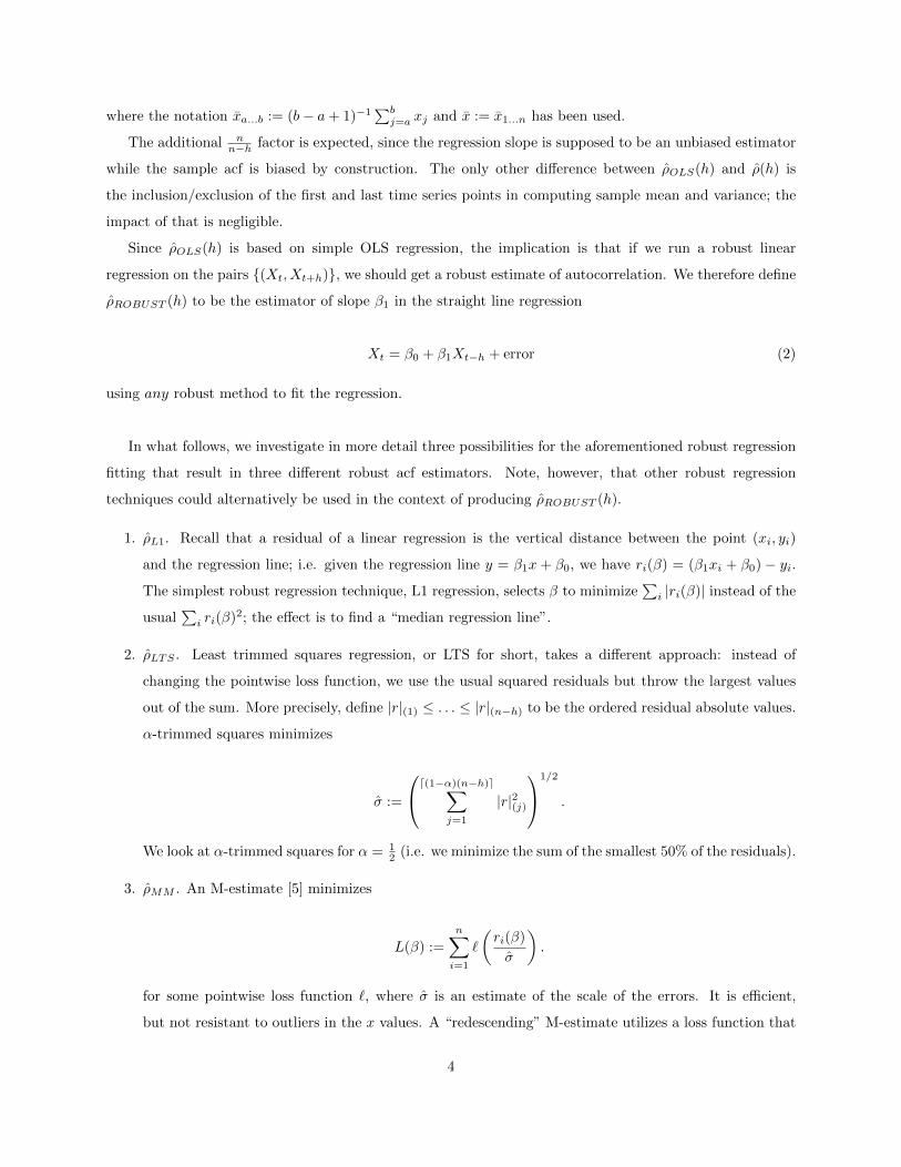
1. ρL1. Recall that a residual of a linear regression is the vertical distance between the point (xi, yi)

and the regression line; i.e. given the regression line y = β1x + β0, we have ri(β) = (β1xi + β0) − yi.

The simplest robust regression technique, L1 regression, selects β to minimize∑i |ri(β)| instead of the

usual∑i ri(β)2; the effect is to find a “median regression line”.

2. ρLTS . Least trimmed squares regression, or LTS for short, takes a different approach: instead of

changing the pointwise loss function, we use the usual squared residuals but throw the largest values

out of the sum. More precisely, define |r|(1) ≤ . . . ≤ |r|(n−h) to be the ordered residual absolute values.

α-trimmed squares minimizes

σ :=

d(1−α)(n−h)e∑j=1

|r|2(j)

1/2

.

We look at α-trimmed squares for α = 12 (i.e. we minimize the sum of the smallest 50% of the residuals).

3. ρMM . An M-estimate [5] minimizes

L(β) :=

n∑i=1

`

(ri(β)

σ

).

for some pointwise loss function `, where σ is an estimate of the scale of the errors. It is efficient,

but not resistant to outliers in the x values. A “redescending” M-estimate utilizes a loss function that

4

decreases to zero at the tails (as opposed to a monotone increasing loss function).

In contrast, an S-estimate (S for “scale”) minimizes a robust estimate of the scale of the residuals:

β := argminβ

σ(r(β))

where r(β) denotes the vector of residuals and σ satisfies

1

n

n−h∑j=1

`(rjσ

)= δ.

(δ is usually chosen to be 12 .) It has superior robustness, but is inefficient.

MM-estimates, pioneered by Yohai [20], combine these two techniques in a way intended to retain the

robustness of S-estimation while gaining the asymptotic efficiency of M-estimation. Specifically, an

initial robust-but-inefficient estimate β0 is computed, then a scale M-estimate of the residuals, and

finally the iteratively reweighted least squares algorithm is used to identify a nearby β that satisfies

the redescending M-estimate equation.

For further discussion on the above three robust regression techniques, see Maronna et al. [13].

3 Theoretical Properties

3.1 General

We focus our attention on normal efficiency and two measures of robustness (breakdown point and in-

fluence function). Relative normal efficiency is the ratio between the asymptotic variance of the classical

estimator and that of another estimator under consideration, assuming Gaussian residuals and no contamina-

tion. This is a measure of the price we are paying for any robustness gains. The breakdown point (BP) is the

asymptotic fraction of points that can be contaminated without entirely masking the original relation. Now,

in the case of time series modeled by ARMA (AutoRegressive Moving Average) processes, we distinguish

two types of outliers [3]:

1. Innovation outliers affect all subsequent observations, and can be observed in a pure ARMA process

with a heavy-tailed innovation distribution.

2. Additive outliers or replacement outliers that exist outside the ARMA process and do not affect other

observations. For second-order stationary data, the difference between the two notions is minimal—a

replacement outlier functions like a slightly variable additive outlier—, so for brevity we just concern

ourselves with additive outliers.

5

●●●●●●●●●●●●●●●●●●●●●●●

●

●●●●●●●●●●●●●●●●●●●●●●●●●

0 200 400 600 800 1000

020

040

060

080

010

00

Single outlier determines regression line

x[i], i=1..49

x[i+

1]

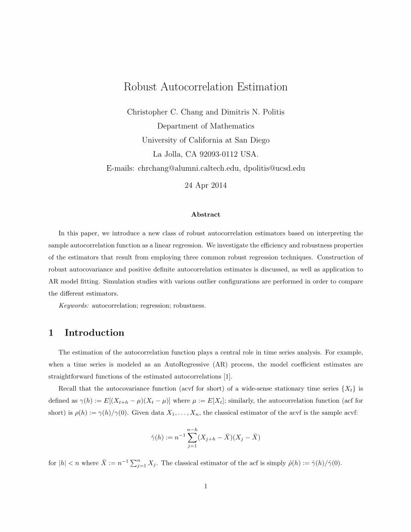
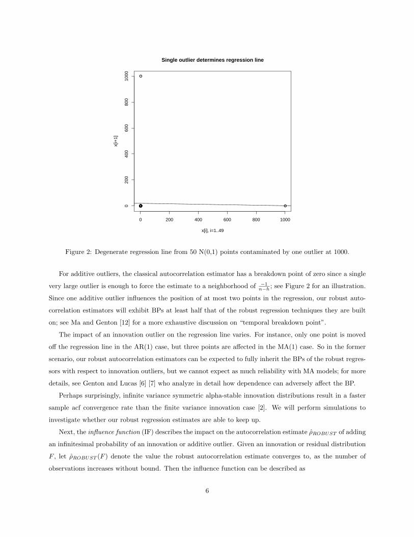
Figure 2: Degenerate regression line from 50 N(0,1) points contaminated by one outlier at 1000.

For additive outliers, the classical autocorrelation estimator has a breakdown point of zero since a single

very large outlier is enough to force the estimate to a neighborhood of −1n−h ; see Figure 2 for an illustration.

Since one additive outlier influences the position of at most two points in the regression, our robust auto-

correlation estimators will exhibit BPs at least half that of the robust regression techniques they are built

on; see Ma and Genton [12] for a more exhaustive discussion on “temporal breakdown point”.

The impact of an innovation outlier on the regression line varies. For instance, only one point is moved

off the regression line in the AR(1) case, but three points are affected in the MA(1) case. So in the former

scenario, our robust autocorrelation estimators can be expected to fully inherit the BPs of the robust regres-

sors with respect to innovation outliers, but we cannot expect as much reliability with MA models; for more

details, see Genton and Lucas [6] [7] who analyze in detail how dependence can adversely affect the BP.

Perhaps surprisingly, infinite variance symmetric alpha-stable innovation distributions result in a faster

sample acf convergence rate than the finite variance innovation case [2]. We will perform simulations to

investigate whether our robust regression estimates are able to keep up.

Next, the influence function (IF) describes the impact on the autocorrelation estimate ρROBUST of adding

an infinitesimal probability of an innovation or additive outlier. Given an innovation or residual distribution

F , let ρROBUST (F ) denote the value the robust autocorrelation estimate converges to, as the number of

observations increases without bound. Then the influence function can be described as

6

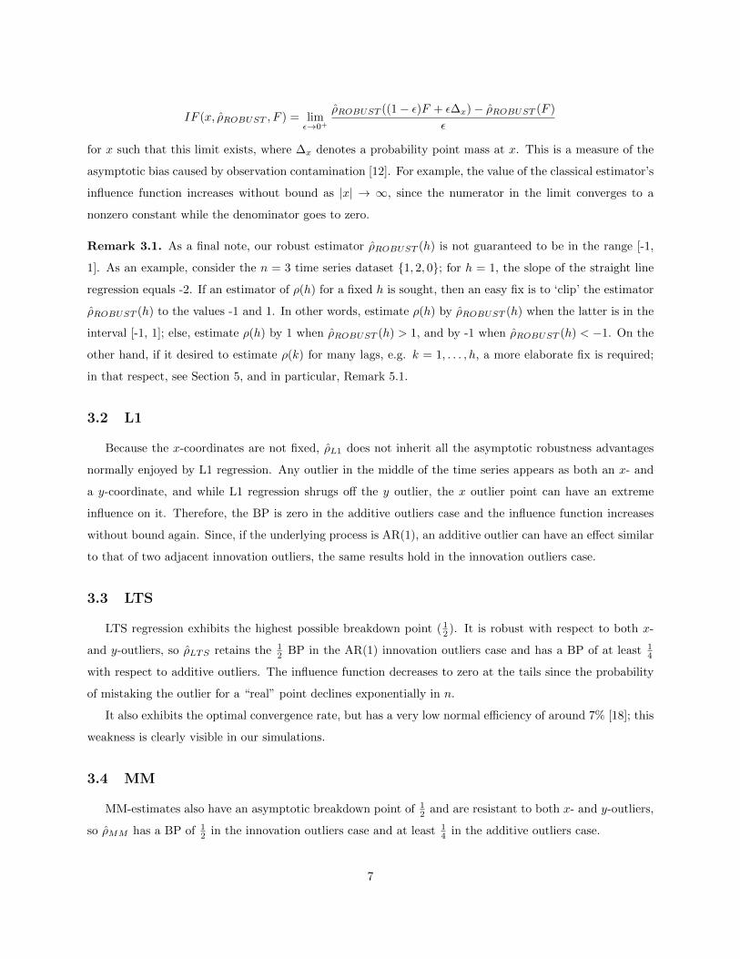
IF (x, ρROBUST , F ) = limε→0+

ρROBUST ((1− ε)F + ε∆x)− ρROBUST (F )

ε

for x such that this limit exists, where ∆x denotes a probability point mass at x. This is a measure of the

asymptotic bias caused by observation contamination [12]. For example, the value of the classical estimator’s

influence function increases without bound as |x| → ∞, since the numerator in the limit converges to a

nonzero constant while the denominator goes to zero.

Remark 3.1. As a final note, our robust estimator ρROBUST (h) is not guaranteed to be in the range [-1,

1]. As an example, consider the n = 3 time series dataset {1, 2, 0}; for h = 1, the slope of the straight line

regression equals -2. If an estimator of ρ(h) for a fixed h is sought, then an easy fix is to ‘clip’ the estimator

ρROBUST (h) to the values -1 and 1. In other words, estimate ρ(h) by ρROBUST (h) when the latter is in the

interval [-1, 1]; else, estimate ρ(h) by 1 when ρROBUST (h) > 1, and by -1 when ρROBUST (h) < −1. On the

other hand, if it desired to estimate ρ(k) for many lags, e.g. k = 1, . . . , h, a more elaborate fix is required;

in that respect, see Section 5, and in particular, Remark 5.1.

3.2 L1

Because the x-coordinates are not fixed, ρL1 does not inherit all the asymptotic robustness advantages

normally enjoyed by L1 regression. Any outlier in the middle of the time series appears as both an x- and

a y-coordinate, and while L1 regression shrugs off the y outlier, the x outlier point can have an extreme

influence on it. Therefore, the BP is zero in the additive outliers case and the influence function increases

without bound again. Since, if the underlying process is AR(1), an additive outlier can have an effect similar

to that of two adjacent innovation outliers, the same results hold in the innovation outliers case.

3.3 LTS

LTS regression exhibits the highest possible breakdown point ( 12 ). It is robust with respect to both x-

and y-outliers, so ρLTS retains the 12 BP in the AR(1) innovation outliers case and has a BP of at least 1

4

with respect to additive outliers. The influence function decreases to zero at the tails since the probability

of mistaking the outlier for a “real” point declines exponentially in n.

It also exhibits the optimal convergence rate, but has a very low normal efficiency of around 7% [18]; this

weakness is clearly visible in our simulations.

3.4 MM

MM-estimates also have an asymptotic breakdown point of 12 and are resistant to both x- and y-outliers,

so ρMM has a BP of 12 in the innovation outliers case and at least 1

4 in the additive outliers case.

7

The normal efficiency is actually a user-adjustable parameter. In practice, it it is usually chosen to

be between 0.7 and 0.95; aiming for an even higher normal efficiency results in too large a region where

the MM-estimate tracks the performance of the classical estimator rather than exhibiting the S-estimate’s

robustness. We use 0.85 in our simulations.

4 Robust autocovariance estimation

Our robust acf estimators can be converted into autocovariance estimators via multiplication by a robust

estimate of variance. This could proceed as follows:

1. First, obtain a robust estimate of location. Building on equation (2), from each autocorrelation regres-

sion we perform, we can derive an estimate of the process mean µ:

Xt − µ = β1(Xt−h − µ) + error, since this line should have zero intercept

Xt = β0 + β1Xt−h + error (3)

where β0 = µ(1− β1) (combining eq. (2) and (3)).

Finally, let µh :=β0

1− β1

where β0, β1 are robust estimates of β0, β1 in the linear regression (3).

2. Each value of h > 0 used in the above step will yield a distinct estimator of location denoted by µh.

We can now use the median of the distinct values µk for k = 1, . . . , (some) p to arrive to a single,

better estimator for µ denoted by µ. For example, we can use L1 notions and take µ as the median of

the values {µk for k = 1, . . . , p}. Alternatively, LTS regression can be applied to µk for k = 1, . . . , p in

order to boil them down to a single estimate.

3. Since (Xt − µ)2 = γ(0) + error, we can robustly estimate γ(0) by using L1 (or LTS) on the centered

sample values (Xt − µ)2 for t = 1, . . . , n. E.g., let γROBUST (0) be the median of (Xt − µ)2 for

t = 1, . . . , n.

4. Finally, we define our robust autocovariance estimator for general h as

γROBUST (h) = ρROBUST (h) · γROBUST (0).

Remark 4.1. The estimators ρROBUST (h) and γROBUST (h) are robust point estimators of the values ρ(h)

and γ(h). To construct confidence intervals and hypothesis tests based on these estimators, an approximation

to their sampling distribution would be required. Such an approximation appears analytically intractable

8

at the moment without imposing assumptions that are so strong to make the whole setting uninteresting,

e.g., assuming that the time series {Xt} is Gaussian. To avoid such unreliastic assumptions, the practitioner

may use a bootstrap approximation to the sampling distribution of the estimators ρROBUST (h) and/or

γROBUST (h). Several powerful resampling methods for time series data have been developed in the last 25

years, e.g., blocking methods, AR-sieve bootstrap, frequency domain methods, etc.; see the recent review by

Kreiss and Paparoditis [10] and the references therein. It is unclear at the moment which of these methods

would be preferable in the context of ρROBUST (h) and γROBUST (h). A benchmark method that typically

works under the weakest assumptions is Subsampling; see Politis, Romano, and Wolf [17].

There are other approaches to robust autocovariance estimation in the literature; see e.g. Ma and Genton

[12] and the references therein.

5 Robust positive definite estimation of autocorrelation matrix

Let Σ denote the n×n matrix with i, j element Σi,j := ρ(|i− j|); in other words, Σ is the autocorrelation

matrix of the data (X1, . . . , Xn) viewed as a vector. An immediate way to robustly estimate the autocor-

relation matrix Σ is by plugging our robust correlation estimates. For example, define a matrix Σ that has

i, j element given by ρROBUST (|i− j|). Although intuitive, Σ is neither consistent for Σ as n→∞, nor is it

positive definite; see Wu and Pourahmadi [19] and the references therein.

Following Politis [16], we may define a ‘flat-top’ taper as the function κ satisfying

κ(x) =

1 if |x| ≤ 1

g(x) if 1 < |x| ≤ cκ0 if |x| > cκ,

where cκ ≥ 1 is a constant, and g(x) is some function such that |g(x)| ≤ 1. Let the taper’s l-scaled version

be denoted as κl(x) := κ(x/l). Taking κ of trapezoidal shape, i.e., letting g(x) = 2− |x| and cκ = 2, yields a

simple taper that has been shown to work well in practice. McMurry and Politis [14] introduced a consistent

estimator of Σ defined as the n × n matrix with i, j element given by κl(i − j)ρ(|i − j|); here, l serves the

role of a bandwidth parameter satisfying l→∞ but l/n→ 0 as n→∞.

In order to “robustify” the tapered estimator of McMurry and Politis [14], we propose Σκ,l as an estimator

of Σ where the i, j element of Σκ,l is given by κl(i − j)ρROBUST (|i − j|). Note, however, that Σκ,l is not

guaranteed to be positive definite. To address this problem, let Σκ,l = TnDTtn be the spectral decomposition

of Σκ,l. Since Σκ,l is symmetric, Tn will be an orthogonal matrix, and D = diag(d1, . . . , dn) which are the

eigenvalues of Σκ,l). Define

D(ε) := diag(d(ε)1 , . . . , d(ε)n ), with d

(ε)i := max(di, ε/n

ζ) (4)

9

where ε ≥ 0 and ζ > 1/2 are two constants. The choices ζ = 1 and ε = 1 works well in practice as in

McMurry and Politis [14].

Finally, we define

Σ(ε)κ,l := TnD

(ε)T tn. (5)

By construction, Σ(ε)κ,l is nonnegative definite when ε = 0, and strictly positive definite when ε > 0. Fur-

thermore, Σ(ε)κ,l inherits the robustness and consistency of Σκ,l. Finally, note that the matrix that equals

γROBUST (0)Σ(ε)κ,l is positive definite, robust and consistent estimator of the autocovariance matrix of the

data (X1, . . . , Xn) viewed as a vector.

Remark 5.1. As mentioned at the end of Section 3.1, the estimator ρROBUST (h) is not necessarily in the

interval [−1, 1]. The construction of the nonnegative definite estimator Σ(ε)κ,l fixes this problem. In particular,

the whole vector of autocorrelations (ρ(0), ρ(1), . . . , ρ(n − 1))—where of course ρ(0) = 1—is estimated by

the first row of matrix Σ(ε)κ,l. As long as ε ≥ 0, this vector estimator can be considered as the the first part

of a nonnegative definite sequence, and hence it can be considered as the first part of the autocorrelation

sequence of some stationary time series; see e.g. Brockwell and Davis (1991). Hence, the vector estimator

enjoys all the properties of an autocorrelation sequence, including the property of belonging to the interval

[−1, 1].

6 Robust AR Model Fitting

6.1 Robust Yule-Walker Estimates

Consider again the causal AR(p) model of eq. (1), i.e., Xt = φ1Xt−1 + . . . + φpXk−p + zt. Now we do

not need to assume that the driving noise zt is iid; it is sufficient that zt is a mean zero, white noise with

variance σ2.

In this context, autocovariance estimates can be directly used to derive AR coefficient estimates via the

Yule-Walker equations:

ˆγ(0) = φ1γ(−1) + . . .+ φpγ(k − p) + σ2

and

ρ(k) = φ1ρ(k − 1) + . . .+ φpρ(k − p) for k = 1, . . . , p. (6)

However, if the classical autocovariance estimates are used in the above, a single outlier of size B perturbs

the φ coefficient estimates by O(B/n); a pair of such outliers can perturb φ1 by O(B2/n).

A simple way to attempt to address this vulnerability is to plug robust autocovariance estimates into the

linear system (6), i.e., to use γROBUST (0) in place of ˆγ(0), and ρROBUST (k) instead of ρ(k). The resulting

10

robust estimate of the coefficient vector φp

:= (φ1, . . . , φp)′ is given by

φp,ROBUST

:= S−1p ρp

(7)

where for any m ≤ n we let ρm

:= (ρROBUST (1), . . . , ρROBUST (m))′

and ρm

:= (ρ(1), . . . , ρ(m))′. Further-

more, in the above, Sp is the upper left p × p submatrix of the autocorrelation matrix Σ(ε)κ,l defined in the

previous section. Since Sp is a Toeplitz matrix, its inverse S−1p can be found via fast algorithms such as the

Durbin-Levinson algorithm.

6.2 Extended Yule-Walker

The ‘extended’ Yule-Walker equations are identical to the usual ones of eq. (6) except letting k =

1, . . . , p′ for some value p′ ≥ p, i.e., they are an overdetermined system: p′ equations with p unknowns

φp

= (φ1, . . . , φp)′. Politis [15] noted that the extended Yule-Walker equations can be used to provide a

more robust estimator of φp. For example, in the AR(1) case with p = 1, letting p′ = 2 suggests that

γ(1)/γ(0) and γ(2)/γ(1) are equally valid as estimators for φ1 that could be combined to yield an improved

one.

Generalizing this idea, fix p′ ≥ p, and let Sp′,p be the p′×p matrix with jth column equal to (ρROBUST (1−

j), ρROBUST (2−j), . . . , ρROBUST (p′−j)); alternatively, we could define Sp′,p as the upper left p′×p submatrix

of the autocorrelation matrix Σ(ε)κ,l defined in Section 5.

As mentioned above, the extended Yule-Walker equations with k = 1, . . . , p′ > p is an overdetermined

system. Thus, we can not expect that ρp′

exactly equals Sp′,pφp. Define the discrepancy η = ρp′− Sp′,pφp

from which it follows that

ρp′

= Sp′,pφp + η. (8)

As suggested by Politis [15] , equation (8) can be viewed as a linear regression (with ‘errors-in-variables’)

having response ρp′

, design matrix Sp′,p, parameter vector φp, and error vector η. Finding OLS estimates of

φp

in the regression model (8) gives doubly robust estimates: robust because ρROBUST (h) were used but also

because of the use of the extended Yule-Walker equations. One could alternatively use a robust regression

technique to fit regression (8); the details are obvious and are omitted.

7 Numerical Work

7.1 Simulation without Outliers

First, we generated time series data X1, . . . , Xn according to the MA(1) model Xt = Zt + φZt−1 (with

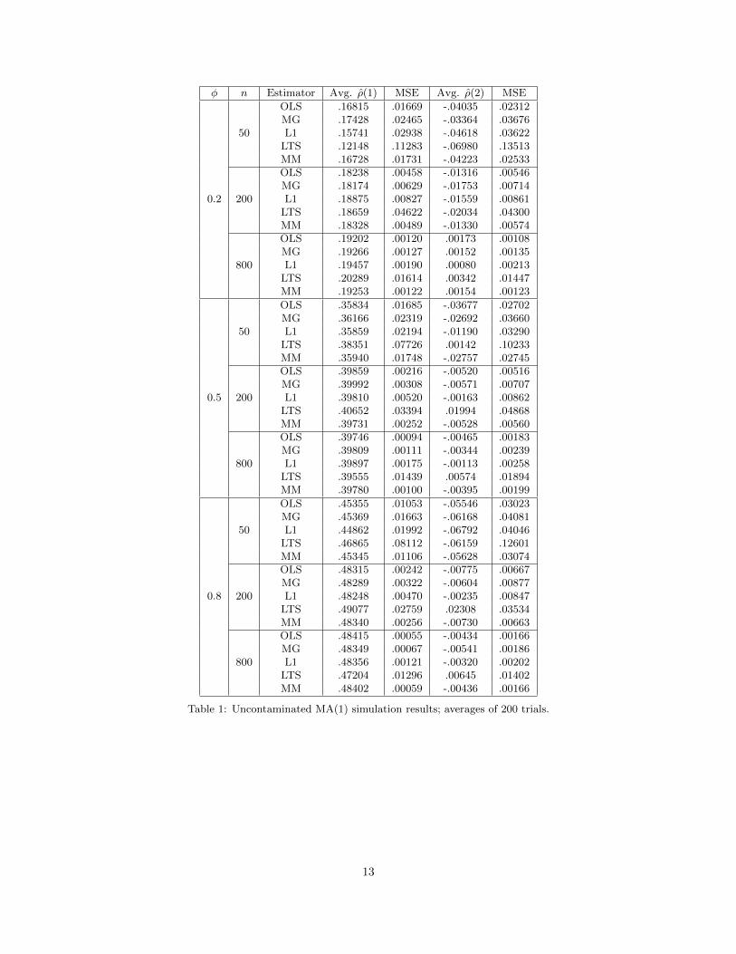
no outliers) with φ ∈ {0.2, 0.5, 0.8}, n ∈ {50, 200, 800}, and Zt i.i.d. N(0, 1). We estimated the lag-1 and

11

lag-2 autocorrelations in different ways, and compared them to the true values ( φ1+φ2 and 0, respectively).

We did the same thing for the AR(1) model Xt = φXt−1 +Zt; the true autocorrelations are φ and φ2 in this

case.

The estimators that were constructed were ρROBUST (h) using the three aforementioned options for

robust regression: L1, LTS and MM. As baselines for comparison, we included Ordinary Least Squares

(OLS) regression, which as discussed above is nearly identical to the sample acf, and Ma and Genton’s [12]

robust autocorrelation estimator (denoted MG).

12

φ n Estimator Avg. ρ(1) MSE Avg. ρ(2) MSE

0.2

50

OLS .16815 .01669 -.04035 .02312MG .17428 .02465 -.03364 .03676L1 .15741 .02938 -.04618 .03622

LTS .12148 .11283 -.06980 .13513MM .16728 .01731 -.04223 .02533

200

OLS .18238 .00458 -.01316 .00546MG .18174 .00629 -.01753 .00714L1 .18875 .00827 -.01559 .00861

LTS .18659 .04622 -.02034 .04300MM .18328 .00489 -.01330 .00574

800

OLS .19202 .00120 .00173 .00108MG .19266 .00127 .00152 .00135L1 .19457 .00190 .00080 .00213

LTS .20289 .01614 .00342 .01447MM .19253 .00122 .00154 .00123

0.5

50

OLS .35834 .01685 -.03677 .02702MG .36166 .02319 -.02692 .03660L1 .35859 .02194 -.01190 .03290

LTS .38351 .07726 .00142 .10233MM .35940 .01748 -.02757 .02745

200

OLS .39859 .00216 -.00520 .00516MG .39992 .00308 -.00571 .00707L1 .39810 .00520 -.00163 .00862

LTS .40652 .03394 .01994 .04868MM .39731 .00252 -.00528 .00560

800

OLS .39746 .00094 -.00465 .00183MG .39809 .00111 -.00344 .00239L1 .39897 .00175 -.00113 .00258

LTS .39555 .01439 .00574 .01894MM .39780 .00100 -.00395 .00199

0.8

50

OLS .45355 .01053 -.05546 .03023MG .45369 .01663 -.06168 .04081L1 .44862 .01992 -.06792 .04046

LTS .46865 .08112 -.06159 .12601MM .45345 .01106 -.05628 .03074

200

OLS .48315 .00242 -.00775 .00667MG .48289 .00322 -.00604 .00877L1 .48248 .00470 -.00235 .00847

LTS .49077 .02759 .02308 .03534MM .48340 .00256 -.00730 .00663

800

OLS .48415 .00055 -.00434 .00166MG .48349 .00067 -.00541 .00186L1 .48356 .00121 -.00320 .00202

LTS .47204 .01296 .00645 .01402MM .48402 .00059 -.00436 .00166

Table 1: Uncontaminated MA(1) simulation results; averages of 200 trials.

13

φ n Estimator Avg. ρ(1) MSE Avg. ρ(2) MSE

0.2

50

OLS .16358 .02592 .02875 .01956MG .15360 .03837 .02700 .03465L1 .17565 .03564 .01710 .03553

LTS .18526 .11907 -.00201 .12429MM .16702 .02758 .02804 .02197

200

OLS .20110 .00439 .02818 .00552MG .20064 .00550 .02512 .00688L1 .19851 .00733 .02330 .00762

LTS .19576 .04101 .02079 .03917MM .20009 .00459 .02691 .00562

800

OLS .19193 .00125 .04054 .00123MG .19286 .00162 .04009 .00146L1 .19139 .00206 .04056 .00211

LTS .19555 .01551 .05124 .01590MM .19191 .00137 .04066 .00124

0.5

50

OLS .44600 .01603 .18352 .02630MG .44176 .02597 .18445 .03796L1 .45312 .02454 .19821 .03591

LTS .46085 .09045 .21308 .11105MM .44471 .01738 .18691 .02687

200

OLS .48241 .00417 .23662 .00681MG .47893 .00494 .23194 .00776L1 .48157 .00635 .23560 .00937

LTS .48630 .03007 .22803 .03912MM .48229 .00429 .23674 .00699

800

OLS .49777 .00100 .24495 .00157MG .49708 .00125 .24396 .00202L1 .49994 .00147 .24465 .00210

LTS .50000 .00983 .24269 .01308MM .49796 .00105 .24512 .00165

0.8

50

OLS .72894 .01682 .52273 .04186MG .70482 .02413 .48780 .05783L1 .72172 .02256 .51311 .05671

LTS .69385 .06811 .49295 .15527MM .72896 .01790 .51800 .04563

200

OLS .78556 .00191 .61795 .00502MG .78135 .00235 .61327 .00565L1 .78586 .00291 .61878 .00646

LTS .78713 .01646 .61040 .03228MM .78498 .00193 .61847 .00489

800

OLS .79622 .00045 .63450 .00142MG .79563 .00052 .63324 .00166L1 .79702 .00076 .63717 .00185

LTS .80020 .00573 .64809 .00765MM .79634 .00048 .63522 .00149

Table 2: Uncontaminated AR(1) simulation results; averages of 200 trials.

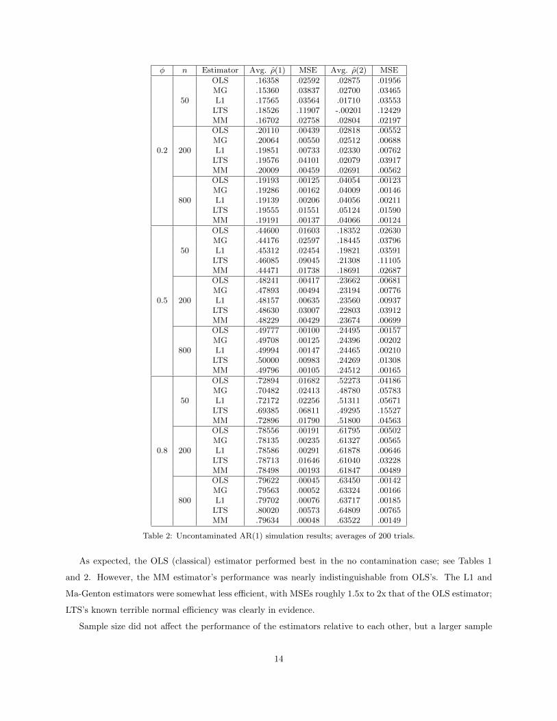
As expected, the OLS (classical) estimator performed best in the no contamination case; see Tables 1

and 2. However, the MM estimator’s performance was nearly indistinguishable from OLS’s. The L1 and

Ma-Genton estimators were somewhat less efficient, with MSEs roughly 1.5x to 2x that of the OLS estimator;

LTS’s known terrible normal efficiency was clearly in evidence.

Sample size did not affect the performance of the estimators relative to each other, but a larger sample

14

size reduced the downward bias of them all.

7.2 Simulation with Innovation Outliers

Next, we investigated estimator performance when faced with innovation outliers, modifying Zt to be

distributed according to a Gaussian mixture, 90 or 96 percent N(0, 1) and 10 or 4 percent N(0, 625).

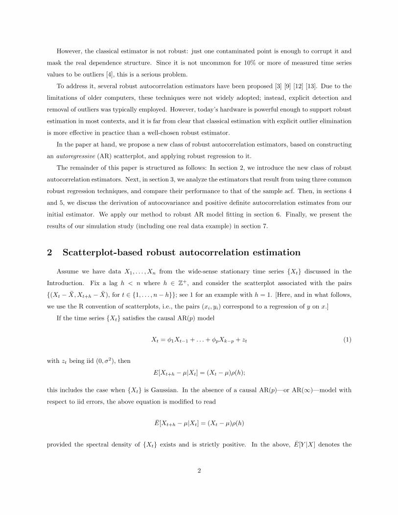
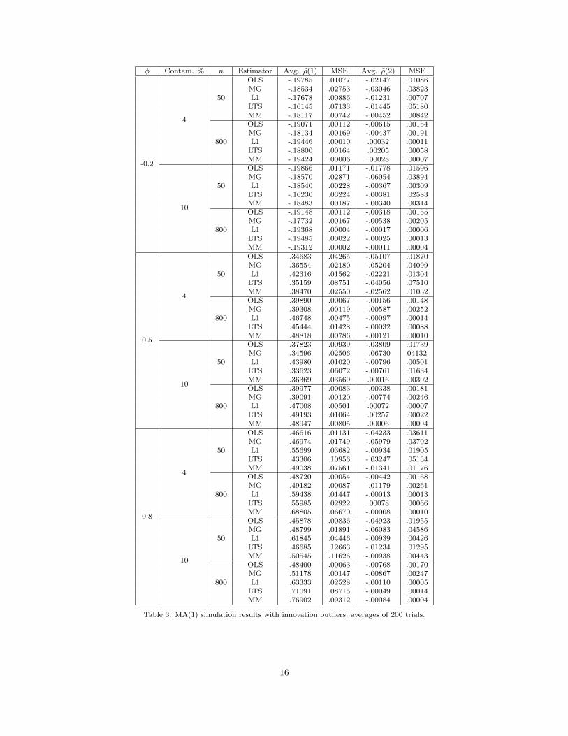
From Table 3 we can see that for φ = −0.2, the Ma-Genton, L1, and MM estimators do a substantially

better job of handling the innovation outliers than the sample acf. However, for larger values of φ and large

sample sizes, our robust estimates of ρ(1) cluster toward φ instead of φ1+φ2 . The reason for that is that any

innovation outlier not immediately followed by a second one creates a point on the scatterplot of the form

(x+ ε1, φx+ ε2) where |x| >> |εi|; all of these high-magnitude points trace a single line of slope φ which are

picked up by the robust estimators as the primary signal, and the other high-magnitude outlier points (which

bring the OLS estimate in line) are ignored. See Figure 3 for an illustration. The Ma-Genton estimator, not

being based on linear regression, is not affected by this pattern.

15

φ Contam. % n Estimator Avg. ρ(1) MSE Avg. ρ(2) MSE

-0.2

4

50

OLS -.19785 .01077 -.02147 .01086MG -.18534 .02753 -.03046 .03823L1 -.17678 .00886 -.01231 .00707LTS -.16145 .07133 -.01445 .05180MM -.18117 .00742 -.00452 .00842

800

OLS -.19071 .00112 -.00615 .00154MG -.18134 .00169 -.00437 .00191L1 -.19446 .00010 .00032 .00011LTS -.18800 .00164 .00205 .00058MM -.19424 .00006 .00028 .00007

10

50

OLS -.19866 .01171 -.01778 .01596MG -.18570 .02871 -.06054 .03894L1 -.18540 .00228 -.00367 .00309LTS -.16230 .03224 -.00381 .02583MM -.18483 .00187 -.00340 .00314

800

OLS -.19148 .00112 -.00318 .00155MG -.17732 .00167 -.00538 .00205L1 -.19368 .00004 -.00017 .00006LTS -.19485 .00022 -.00025 .00013MM -.19312 .00002 -.00011 .00004

0.5

4

50

OLS .34683 .04265 -.05107 .01870MG .36554 .02180 -.05204 .04099L1 .42316 .01562 -.02221 .01304LTS .35159 .08751 -.04056 .07510MM .38470 .02550 -.02562 .01032

800

OLS .39890 .00067 -.00156 .00148MG .39308 .00119 -.00587 .00252L1 .46748 .00475 -.00097 .00014LTS .45444 .01428 -.00032 .00088MM .48818 .00786 -.00121 .00010

10

50

OLS .37823 .00939 -.03809 .01739MG .34596 .02506 -.06730 04132L1 .43980 .01020 -.00796 .00501LTS .33623 .06072 -.00761 .01634MM .36369 .03569 .00016 .00302

800

OLS .39977 .00083 -.00338 .00181MG .39091 .00120 -.00774 .00246L1 .47008 .00501 .00072 .00007LTS .49193 .01064 .00257 .00022MM .48947 .00805 .00006 .00004

0.8

4

50

OLS .46616 .01131 -.04233 .03611MG .46974 .01749 -.05979 .03702L1 .55699 .03682 -.00934 .01905LTS .43306 .10956 -.03247 .05134MM .49038 .07561 -.01341 .01176

800

OLS .48720 .00054 -.00442 .00168MG .49182 .00087 -.01179 .00261L1 .59438 .01447 -.00013 .00013LTS .55985 .02922 .00078 .00066MM .68805 .06670 -.00008 .00010

10

50

OLS .45878 .00836 -.04923 .01955MG .48799 .01891 -.06083 .04586L1 .61845 .04446 -.00939 .00426LTS .46685 .12663 -.01234 .01295MM .50545 .11626 -.00938 .00443

800

OLS .48400 .00063 -.00768 .00170MG .51178 .00147 -.00867 .00247L1 .63333 .02528 -.00110 .00005LTS .71091 .08715 -.00049 .00014MM .76902 .09312 -.00084 .00004

Table 3: MA(1) simulation results with innovation outliers; averages of 200 trials.

16

-60 -40 -20 0 20 40 60

-60

-40

-20

020

4060

MA(1) (phi=0.8, n=800) with innovation outliers

x[i], i=1..799

x[i+1]

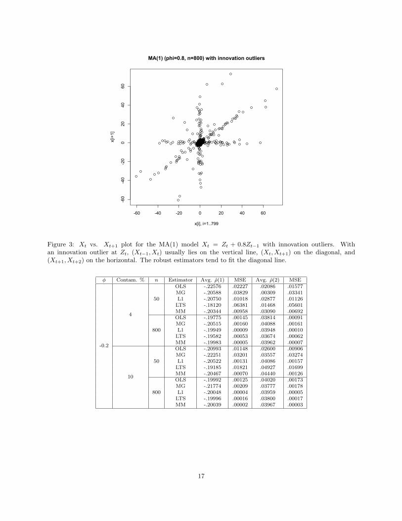
Figure 3: Xt vs. Xt+1 plot for the MA(1) model Xt = Zt + 0.8Zt−1 with innovation outliers. Withan innovation outlier at Zt, (Xt−1, Xt) usually lies on the vertical line, (Xt, Xt+1) on the diagonal, and(Xt+1, Xt+2) on the horizontal. The robust estimators tend to fit the diagonal line.

φ Contam. % n Estimator Avg. ρ(1) MSE Avg. ρ(2) MSE

-0.2

4

50

OLS -.22576 .02227 .02086 .01577MG -.20588 .03829 .00309 .03341L1 -.20750 .01018 .02877 .01126LTS -.18120 .06381 .01468 .05601MM -.20344 .00958 .03090 .00692

800

OLS -.19775 .00145 .03814 .00091MG -.20515 .00160 .04088 .00161L1 -.19949 .00009 .03948 .00010LTS -.19582 .00053 .03674 .00062MM -.19983 .00005 .03962 .00007

10

50

OLS -.20993 .01148 .02600 .00906MG -.22251 .03201 .03557 .03274L1 -.20522 .00131 .04086 .00157LTS -.19185 .01821 .04927 .01699MM -.20467 .00070 .04440 .00126

800

OLS -.19992 .00125 .04020 .00173MG -.21774 .00209 .03777 .00178L1 -.20048 .00004 .03959 .00005LTS -.19996 .00016 .03800 .00017MM -.20039 .00002 .03967 .00003

17

φ Contam. % n Estimator Avg. ρ(1) MSE Avg. ρ(2) MSE

0.5

4

50

OLS .46520 .00956 .19043 .02019MG .48690 .02355 .19364 .04024L1 .49198 .00532 .22763 .00791LTS .48511 .02905 .19989 .04247MM .49183 .00377 .23505 .00649

800

OLS .49840 .00097 .24964 .00152MG .53888 .00282 .26705 .00255L1 .49969 .00006 .25023 .00009LTS .50038 .00039 .25076 .00039MM .49966 .00004 .24984 .00007

10

50

OLS .43619 .04085 .17919 .02531MG .55736 .02541 .23512 .03739L1 .48964 .00309 .23227 .00662LTS .48506 .00814 .24911 .01338MM .49613 .00106 .24566 .00249

800

OLS .49832 .00086 .24440 .00151MG .59379 .00993 .28994 .00367L1 .49924 .00003 .24811 .00007LTS .49902 .00012 .24713 .00018MM .49941 .00002 .24885 .00004

0.8

4

50

OLS .74099 .01184 .53776 .03219MG .81219 .01316 .61055 .03626L1 .77752 .00572 .59431 .01536LTS .76933 .02006 .59469 .03543MM .77987 .00425 .59493 .01619

800

OLS .79691 .63449 .00037 .00104MG .88504 .00760 .74106 .01129L1 .80011 .00003 .63971 .00008LTS .80013 .00016 .64059 .00040MM .80001 .00002 .64043 .00006

10

50

OLS .72992 .01731 .53105 .03459MG .89090 .01489 .70164 .02350L1 .79232 .00165 .61721 .00596LTS .79450 .00806 .61635 .01611MM .79677 .00068 .62704 .00465

800

OLS .79714 .00046 .63659 .00137MG .93719 .01892 .80715 .02847L1 .79990 .00001 .63971 .00004LTS .79943 .00008 .64034 .00012MM .80009 .00001 .64031 .00003

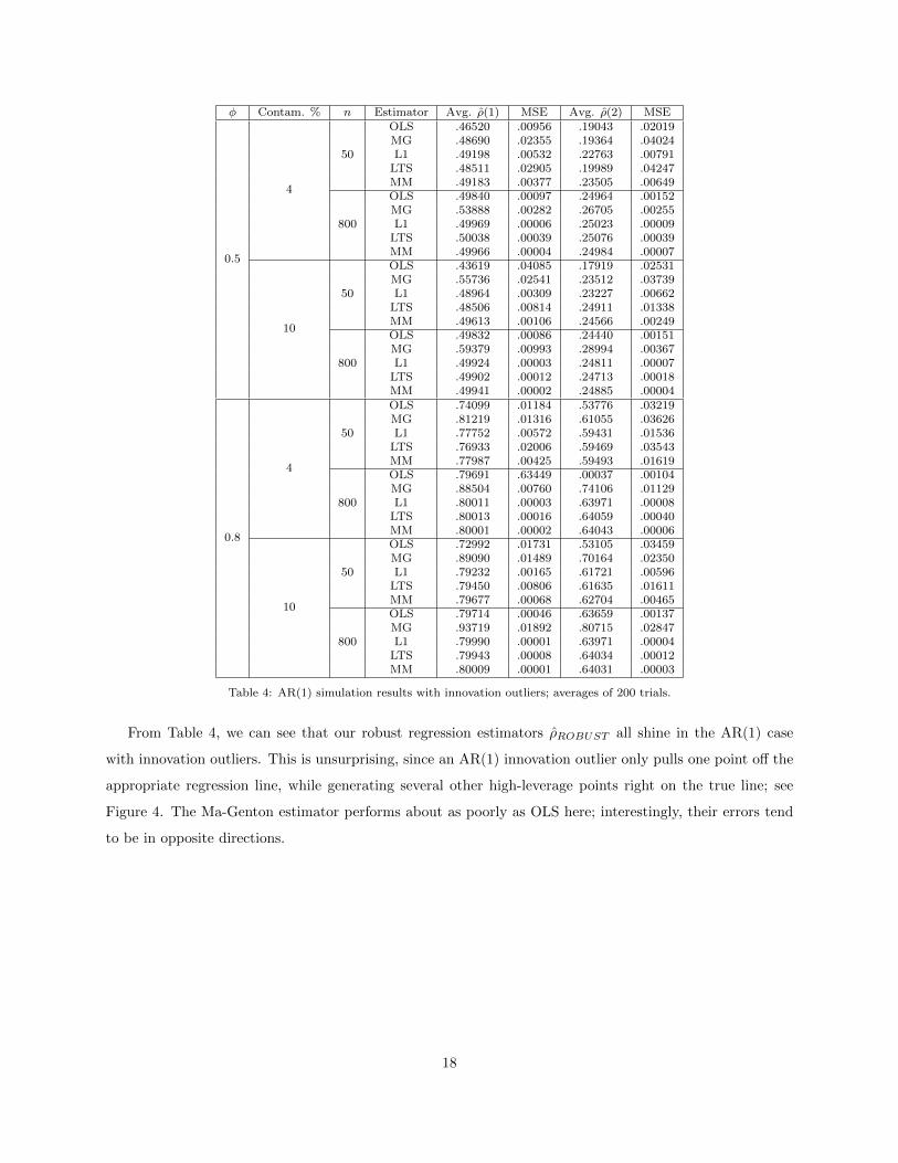
Table 4: AR(1) simulation results with innovation outliers; averages of 200 trials.

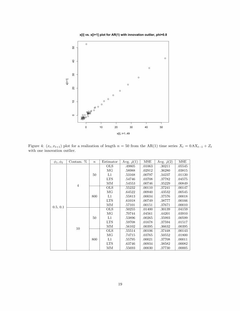
From Table 4, we can see that our robust regression estimators ρROBUST all shine in the AR(1) case

with innovation outliers. This is unsurprising, since an AR(1) innovation outlier only pulls one point off the

appropriate regression line, while generating several other high-leverage points right on the true line; see

Figure 4. The Ma-Genton estimator performs about as poorly as OLS here; interestingly, their errors tend

to be in opposite directions.

18

0 10 20 30 40 50

010

2030

4050

x[i] vs. x[i+1] plot for AR(1) with innovation outlier, phi=0.8

x[i], i=1..49

x[i+1]

Figure 4: (xt, xt+1) plot for a realization of length n = 50 from the AR(1) time series Xt = 0.8Xt−1 + Ztwith one innovation outlier.

φ1, φ2 Contam. % n Estimator Avg. ρ(1) MSE Avg. ρ(2) MSE

0.5, 0.1

4

50

OLS .49805 .01063 .30211 .05545MG .58988 .02912 .36280 .03815L1 .53168 .00797 .34237 .01120

LTS .54746 .03708 .37782 .04575MM .54553 .00746 .35229 .00849

800

OLS .55232 .00110 .37241 .00147MG .64522 .00940 .43532 .00545L1 .55813 .00034 .37576 .00018

LTS .61018 .00749 .38777 .00166MM .57101 .00151 .37671 .00010

10

50

OLS .50255 .01400 .30139 .04159MG .70744 .04561 .44201 .03910L1 .53896 .00265 .35993 .00599

LTS .59708 .01678 .37594 .01517MM .56102 .00395 .36632 .00395

800

OLS .55514 .00106 .37448 .00143MG .74715 .03765 .50552 .01800L1 .55795 .00021 .37708 .00011

LTS .63746 .00934 .38582 .00082MM .55693 .00030 .37730 .00005

19

φ1, φ2 Contam. % n Estimator Avg. ρ(1) MSE Avg. ρ(2) MSE

0.6, 0.3

4

50

OLS .73869 .02945 .66437 .04485MG .85771 .01835 .79481 .03038L1 .83786 .01150 .75807 .02043

LTS .85036 .02913 .77909 .03403MM .85324 .01226 .77049 .01785

800

OLS .85081 .00060 .80749 .00101MG .96729 .01227 .94209 .01663L1 .90582 .00242 .83797 .00066

LTS .91584 .00372 .84984 .00160MM .91882 .00383 .84796 .00121

10

50

OLS .70326 .04351 .62912 .05943MG .91934 .01062 .86392 .01527L1 .84315 .00793 .76536 .01284

LTS .88486 .01410 .81898 .01243MM .88306 .00714 .78694 .00987

800

OLS .84891 .00076 .80323 .00119MG .98441 .01621 .96065 .02146L1 .90649 .00248 .83758 .00062

LTS .92019 .00409 .85299 .00166MM .92185 .00421 .84226 .00084

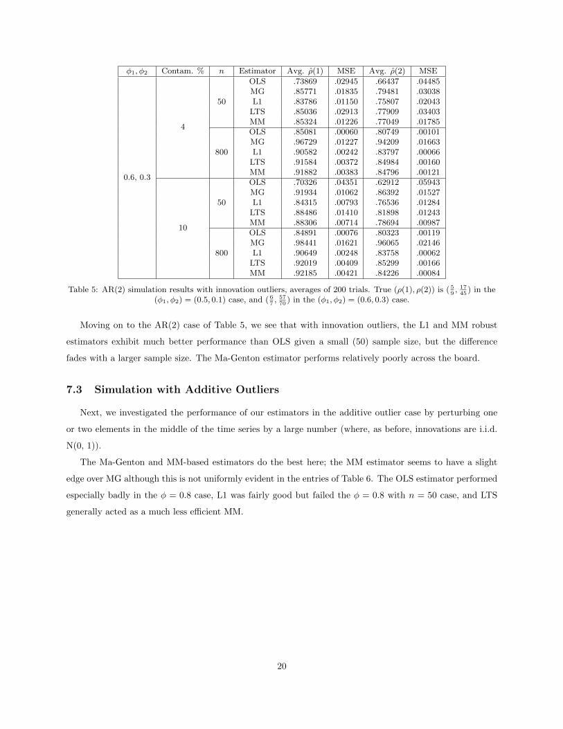
Table 5: AR(2) simulation results with innovation outliers, averages of 200 trials. True (ρ(1), ρ(2)) is ( 59, 1745

) in the(φ1, φ2) = (0.5, 0.1) case, and ( 6

7, 5770

) in the (φ1, φ2) = (0.6, 0.3) case.

Moving on to the AR(2) case of Table 5, we see that with innovation outliers, the L1 and MM robust

estimators exhibit much better performance than OLS given a small (50) sample size, but the difference

fades with a larger sample size. The Ma-Genton estimator performs relatively poorly across the board.

7.3 Simulation with Additive Outliers

Next, we investigated the performance of our estimators in the additive outlier case by perturbing one

or two elements in the middle of the time series by a large number (where, as before, innovations are i.i.d.

N(0, 1)).

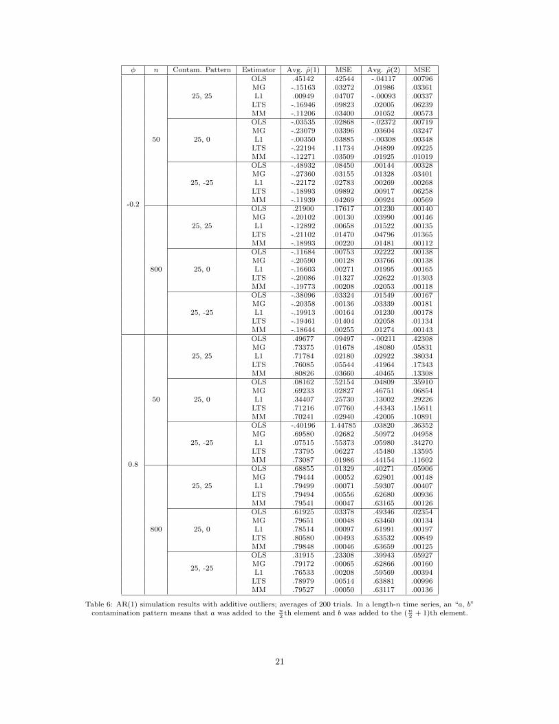
The Ma-Genton and MM-based estimators do the best here; the MM estimator seems to have a slight

edge over MG although this is not uniformly evident in the entries of Table 6. The OLS estimator performed

especially badly in the φ = 0.8 case, L1 was fairly good but failed the φ = 0.8 with n = 50 case, and LTS

generally acted as a much less efficient MM.

20

φ n Contam. Pattern Estimator Avg. ρ(1) MSE Avg. ρ(2) MSE

-0.2

50

25, 25

OLS .45142 .42544 -.04117 .00796MG -.15163 .03272 .01986 .03361L1 .00949 .04707 -.00093 .00337LTS -.16946 .09823 .02005 .06239MM -.11206 .03400 .01052 .00573

25, 0

OLS -.03535 .02868 -.02372 .00719MG -.23079 .03396 .03604 .03247L1 -.00350 .03885 -.00308 .00348LTS -.22194 .11734 .04899 .09225MM -.12271 .03509 .01925 .01019

25, -25

OLS -.48932 .08450 .00144 .00328MG -.27360 .03155 .01328 .03401L1 -.22172 .02783 .00269 .00268LTS -.18993 .09892 .00917 .06258MM -.11939 .04269 .00924 .00569

800

25, 25

OLS .21900 .17617 .01230 .00140MG -.20102 .00130 .03990 .00146L1 -.12892 .00658 .01522 .00135LTS -.21102 .01470 .04796 .01365MM -.18993 .00220 .01481 .00112

25, 0

OLS -.11684 .00753 .02222 .00138MG -.20590 .00128 .03766 .00138L1 -.16603 .00271 .01995 .00165LTS -.20086 .01327 .02622 .01303MM -.19773 .00208 .02053 .00118

25, -25

OLS -.38096 .03324 .01549 .00167MG -.20358 .00136 .03339 .00181L1 -.19913 .00164 .01230 .00178LTS -.19461 .01404 .02058 .01134MM -.18644 .00255 .01274 .00143

0.8

50

25, 25

OLS .49677 .09497 -.00211 .42308MG .73375 .01678 .48080 .05831L1 .71784 .02180 .02922 .38034LTS .76085 .05544 .41964 .17343MM .80826 .03660 .40465 .13308

25, 0

OLS .08162 .52154 .04809 .35910MG .69233 .02827 .46751 .06854L1 .34407 .25730 .13002 .29226LTS .71216 .07760 .44343 .15611MM .70241 .02940 .42005 .10891

25, -25

OLS -.40196 1.44785 .03820 .36352MG .69580 .02682 .50972 .04958L1 .07515 .55373 .05980 .34270LTS .73795 .06227 .45480 .13595MM .73087 .01986 .44154 .11602

800

25, 25

OLS .68855 .01329 .40271 .05906MG .79444 .00052 .62901 .00148L1 .79499 .00071 .59307 .00407LTS .79494 .00556 .62680 .00936MM .79541 .00047 .63165 .00126

25, 0

OLS .61925 .03378 .49346 .02354MG .79651 .00048 .63460 .00134L1 .78514 .00097 .61991 .00197LTS .80580 .00493 .63532 .00849MM .79848 .00046 .63659 .00125

25, -25

OLS .31915 .23308 .39943 .05927MG .79172 .00065 .62866 .00160L1 .76533 .00208 .59569 .00394LTS .78979 .00514 .63881 .00996MM .79527 .00050 .63117 .00136

Table 6: AR(1) simulation results with additive outliers; averages of 200 trials. In a length-n time series, an “a, b”contamination pattern means that a was added to the n

2th element and b was added to the (n

2+ 1)th element.

21

0 20 40 60 80

89

1011

month

annu

al %

rate

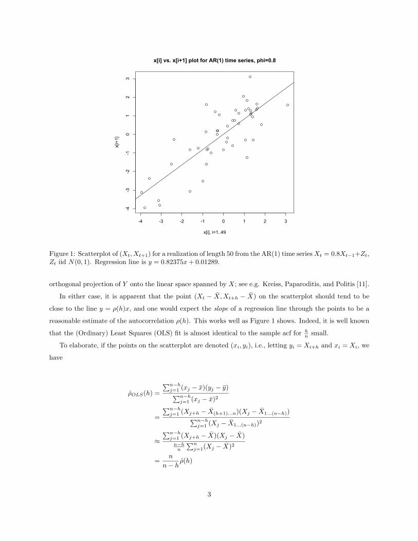
Figure 5: Austrian bank data.

7.4 Real Data Experiment: Austrian Bank Interest Rates

We also applied our robust estimators to some real-world data, namely monthly interest rates of an

Austrian bank over a 91 month period; this data set has been previously discussed and analyzed by Kunsch

[9], Ma and Genton [12], and Genton and Ruiz-Gazen [8]. The outliers around months 20 and 30 are clearly

notable in Figure 5. Table 7 summarizes our findings.

Estimator Outliers replaced? ρ(1) ρ(3) ρ(4) ρ(5) ρ(6) ρ(12)

OLSno .79184 .58923 .51249 .44414 .40440 .08583yes .93911 .77912 .67222 .58084 .49877 .07229

MG no .96571 .82703 .73727 .65968 .55046 -.18033L1 no .97222 .83459 .78351 .72603 .65957 -.02786

LTS no .99451 .95588 .87975 .85556 .36749 -.94203MM no .97194 .81113 .49292 .40119 .34198 .04550

Table 7: Numerical results with Austrian bank data.

The L1 and MM estimates of typical month-to-month and season-to-season autocorrelation are more

reasonable than the OLS estimate which is overly affected by the outliers. However, the LTS estimator was

erratic, overestimating the low lag autocorrelations and yielding a bizarre value of -.94203 for the 12-month

autocorrelation.

22

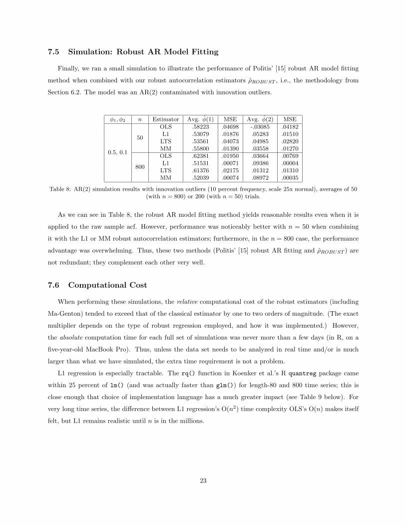
7.5 Simulation: Robust AR Model Fitting

Finally, we ran a small simulation to illustrate the performance of Politis’ [15] robust AR model fitting

method when combined with our robust autocorrelation estimators ρROBUST , i.e., the methodology from

Section 6.2. The model was an AR(2) contaminated with innovation outliers.

φ1, φ2 n Estimator Avg. φ(1) MSE Avg. φ(2) MSE

0.5, 0.1

50

OLS .58223 .04698 -.03085 .04182L1 .53079 .01876 .05283 .01510

LTS .53561 .04073 .04985 .02820MM .55800 .01390 .03558 .01270

800

OLS .62381 .01950 .03664 .00769L1 .51531 .00071 .09386 .00004

LTS .61376 .02175 .01312 .01310MM .52039 .00074 .08972 .00035

Table 8: AR(2) simulation results with innovation outliers (10 percent frequency, scale 25x normal), averages of 50(with n = 800) or 200 (with n = 50) trials.

As we can see in Table 8, the robust AR model fitting method yields reasonable results even when it is

applied to the raw sample acf. However, performance was noticeably better with n = 50 when combining

it with the L1 or MM robust autocorrelation estimators; furthermore, in the n = 800 case, the performance

advantage was overwhelming. Thus, these two methods (Politis’ [15] robust AR fitting and ρROBUST ) are

not redundant; they complement each other very well.

7.6 Computational Cost

When performing these simulations, the relative computational cost of the robust estimators (including

Ma-Genton) tended to exceed that of the classical estimator by one to two orders of magnitude. (The exact

multiplier depends on the type of robust regression employed, and how it was implemented.) However,

the absolute computation time for each full set of simulations was never more than a few days (in R, on a

five-year-old MacBook Pro). Thus, unless the data set needs to be analyzed in real time and/or is much

larger than what we have simulated, the extra time requirement is not a problem.

L1 regression is especially tractable. The rq() function in Koenker et al.’s R quantreg package came

within 25 percent of lm() (and was actually faster than glm()) for length-80 and 800 time series; this is

close enough that choice of implementation language has a much greater impact (see Table 9 below). For

very long time series, the difference between L1 regression’s O(n2) time complexity OLS’s O(n) makes itself

felt, but L1 remains realistic until n is in the millions.

23

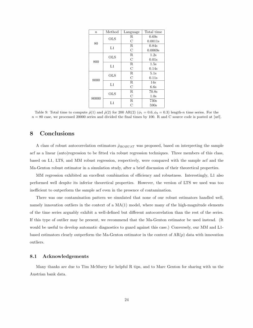
n Method Language Total time

80OLS

R 0.69sC 0.0011s

L1R 0.84sC 0.0069s

800OLS

R 1.2sC 0.01s

L1R 1.5sC 0.14s

8000OLS

R 5.1sC 0.11s

L1R 14sC 6.6s

80000OLS

R 70.8sC 1.0s

L1R 730sC 590s

Table 9: Total time to compute ρ(1) and ρ(2) for 200 AR(2) (φ1 = 0.6, φ2 = 0.3) length-n time series. For then = 80 case, we processed 20000 series and divided the final times by 100. R and C source code is posted at [url].

8 Conclusions

A class of robust autocorrelation estimators ρROBUST was proposed, based on interpreting the sample

acf as a linear (auto)regression to be fitted via robust regression techniques. Three members of this class,

based on L1, LTS, and MM robust regression, respectively, were compared with the sample acf and the

Ma-Genton robust estimator in a simulation study, after a brief discussion of their theoretical properties.

MM regression exhibited an excellent combination of efficiency and robustness. Interestingly, L1 also

performed well despite its inferior theoretical properties. However, the version of LTS we used was too

inefficient to outperform the sample acf even in the presence of contamination.

There was one contamination pattern we simulated that none of our robust estimators handled well,

namely innovation outliers in the context of a MA(1) model, where many of the high-magnitude elements

of the time series arguably exhibit a well-defined but different autocorrelation than the rest of the series.

If this type of outlier may be present, we recommend that the Ma-Genton estimator be used instead. (It

would be useful to develop automatic diagnostics to guard against this case.) Conversely, our MM and L1-

based estimators clearly outperform the Ma-Genton estimator in the context of AR(p) data with innovation

outliers.

8.1 Acknowledgements

Many thanks are due to Tim McMurry for helpful R tips, and to Marc Genton for sharing with us the

Austrian bank data.

24

References

[1] Brockwell, P.J. and Davis, R.A., Time Series: Theory and Methods, Springer, New York, 1991.

[2] Davis, R.A. and Mikosch, T., “The sample autocorrelations of financial time series models,” Nonlinear

and Nonstationary Signal Processing, Cambridge University Press, Cambridge, pp. 247–274, 2000.

[3] Denby, L. and Martin, R.D., ‘Robust estimation of the first-order autoregressive parameter,’ Journal of

the American Statistical Association, vol. 74, no. 365, pp. 140–146, 1979.

[4] Hampel, F.R. ‘Robust estimation, a condensed partial survey’, Zeitschrift fur Wahrscheinlichkeitstheorie

und verwandte Gebiete, vol. 27, pp. 87–104, 1973.

[5] Huber, P.J. ‘Robust regression: Asymptotics, conjectures and Monte Carlo’, Annals of Statistics, vol.

1, pp. 799–821, 1973.

[6] Genton, M. G., and Lucas, A. (2003), ‘Comprehensive definitions of breakdown-points for independent

and dependent observations,’ Journal of the Royal Statistical Society, Series B, vol. 65, 81-94.

[7] Genton, M. G., and Lucas, A. (2005), ‘Discussion of the paper ”Breakdown and groups” by L. Davies

and U. Gather’, Annals of Statistics, vol. 33, 988-993.

[8] Genton, M. G., and Ruiz-Gazen, A. (2010), ‘Visualizing influential observations in dependent data,’ it

Journal of Computational and Graphical Statistics, vol. 19, 808-825.

[9] Kunsch, H. ‘Infinitesimal robustness for autoregressive processes’, Ann. Statist., vol. 12, pp. 843–863,

1984.

[10] Kreiss, J.-P., and Paparoditis, E. ‘Bootstrap methods for dependent data: A review.’ Journal of the

Korean Statistical Society, vol. 40, no. 4, pp. 357-378, 2011.

[11] Kreiss, J.-P., Paparoditis, E. and Politis, D.N. ‘On the Range of Validity of the Autoregressive Sieve

Bootstrap’, Ann. Statist., vol. 39, No. 4, pp. 2103-2130, 2011.

[12] Ma, Y. and Genton, M.G., “Highly robust estimation of the autocovariance function,” Journal of Time

Series Analysis, vol. 21, no. 6, pp. 663–684, 2000.

[13] Maronna, R.A., Martin, R.D., and Yohai, V.J., Robust Statistics: Theory and Methods, Wiley, 2006.

[14] McMurry, T. and Politis, D.N., “Banded and tapered estimates of autocovariance matrices and the

linear process bootstrap,” Journal of Time Series Analysis, vol. 31, pp. 471-482, 2010. [Corrigendum:

vol. 33, 2012.]

25

[15] Politis, D.N., “An algorithm for robust fitting of autoregressive models,” Economics Letters, vol. 102,

no. 2, pp. 128–131, 2009.

[16] Politis, D.N., ‘Higher-order accurate, positive semi-definite estimation of large-sample covariance and

spectral density matrices’, Econometric Theory, vol. 27, no. 4, pp. 703-744, 2011.

[17] Politis, D.N., Romano, J.P. and Wolf, M. Subsampling, Springer, New York, 1999.

[18] Rousseeuw, P.J. and Leroy, A.M., Robust Regression and Outlier Detection, John Wiley & Sons, New

York, 1987.

[19] Wu, W.B. and Pourahmadi, M., “Banding sample autocovariance matrices of stationary processes,”

Statistica Sinica, vol. 19, no. 4, pp. 1755–1768, 2009.

[20] Yohai, V.J., “High breakdown-point and high efficiency estimates for regression,” The Annals of Statis-

tics, vol. 15, pp. 642–656, 1987.

26