Robust Assortment Optimization in Revenue Management … · maintain comparable average revenue if average revenue is the performance measure of interest. 1. Introduction A traditional

Robust Assortment Optimization in Revenue Management

Under the Multinomial Logit Choice Model

Paat Rusmevichientong∗ Huseyin Topaloglu†

September 20, 2011

Abstract

We study robust formulations of assortment optimization problems under the multinomial logit choicemodel. The novel aspect of our formulations is that the true parameters of the logit model are assumedto be unknown, and we represent the set of likely parameter values by a compact uncertainty set. Theobjective is to find an assortment that maximizes the worst case expected revenue over all parametervalues in the uncertainty set. We consider both static and dynamic settings. The static settingignores inventory consideration, while in the dynamic setting, there is a limited initial inventory thatmust be allocated over time. We give a complete characterization of the optimal policy in bothsettings, show that it can be computed efficiently, and derive operational insights. We also propose afamily of uncertainty sets that enables the decision maker to control the tradeoff between increasingthe average revenue and protecting against the worst case scenario. Numerical experiments show thatour robust approach, combined with our proposed family of uncertainty sets, is especially beneficialwhen there is significant uncertainty in the parameter values. When compared to other methods,our robust approach yields over 10% improvement in the worst case performance, but it can alsomaintain comparable average revenue if average revenue is the performance measure of interest.

1. Introduction

A traditional assumption in the revenue management literature has been that each customer arrives

into the system with the intention of purchasing a fixed product. If this product is available, then the

customer makes a purchase; otherwise, he leaves the system without purchasing anything. In many

applications, however, the customer observes a set of available products and makes a selection among

them. In this case, the firm needs to decide which assortment of products to offer, taking into account

the choice process of the customers. The seminal work of Talluri and van Ryzin (2004) has demonstrated

the importance of incorporating customer choice behavior into revenue management models. Since their

formulation of the single leg airline seat allocation problem under a general discrete choice model, there

has been a large amount of research on choice-based revenue management models. Most of this work

assumes that the parameters of the underlying choice model are either known in advance or have been

estimated from data. The revenue management decision is then computed based on the estimated

parameter values, ignoring any uncertainty associated with the estimates. Currently, existing models

do not take into account the losses that may incur when the estimated values differ significantly from

the true parameter values.

∗School of Operations Research and Information Engineering, Cornell University, Ithaca, NY 14853, USA. E-mail:[email protected]

†School of Operations Research and Information Engineering, Cornell University, Ithaca, NY 14853, USA. E-mail:[email protected]

1

In this paper, we formulate assortment optimization models that explicitly incorporate the

uncertainty in the choice parameters. We consider a setting where the set of products is indexed

by A = {1, . . . , n}, and the revenue of each product is ordered such that r1 ≥ r2 ≥ · · · ≥ rn > 0.

The customer choices are driven by the multinomial logit model. However, the parameters of the logit

model are unknown, and the set of likely parameter values is described by a compact uncertainty set.

Our goal is to choose an assortment that maximizes the worst case expected revenue, where the worst

case is taken over all likely parameter values. We consider both static and dynamic settings. The static

setting ignores inventory consideration, while in the dynamic setting, we have a fixed initial inventory

that has to be allocated to customers arriving over time. As described below, we make contributions in

understanding the policy structure, developing efficient computational methods, and deriving important

operational insights.

We consider the static problem in Section 3. When the parameters of the logit model are known

in advance, Talluri and van Ryzin (2004) show that assortments of the form {1, 2, . . . , i} for some

product i are optimal. We call such assortments as revenue-ordered assortments. Surprisingly, we are

able to show that revenue-ordered assortments remain optimal, even when we are uncertain about the

model parameters and we wish to protect against the worst case expected revenue (Theorem 3.2). This

result shows that we can compute the robust assortment efficiently because we only need to consider n

revenue-ordered assortments, instead of all 2n subsets. In addition to generalizing the result of Talluri

and van Ryzin (2004), our proof of Theorem 3.2 is novel and different from the existing techniques in

the literature, contributing to a new understanding of the logit model (Lemma 3.1).

In addition to characterizing the policy structure and providing efficient computational methods,

our analysis provides operational insights about how to protect against uncertainty in the model

parameters. In Corollary 3.5, we show that larger uncertainty leads to a larger robust assortment. Thus,

product variety serves as a buffer against worst case scenario. Moreover, if a firm is operating in a

market with multiple customer segments, then to maximize the worst case expected revenue, it should

target the customer segment whose corresponding preference profile gives rise to the largest optimal

assortment (Theorem 3.6). We also show that firms that carry higher revenue-generating products and

face uncertainty in the marketplace would benefit from offering larger assortments (Theorem 3.7). In

Section 3.3, we propose a family of uncertainty sets that enables the decision maker to control the

tradeoff between increasing the average revenue and protecting against the worst case scenario. The

uncertainty sets we propose are characterized by a radius parameter ϵ. Large values of ϵ provide large

uncertainty sets, resulting in conservative assortments that protect well against the worst case expected

revenue, but lack in average performance. Small values of ϵ provide aggressive assortments with high

average performance, but these assortments may not perform well in terms of the worst case expected

revenue. Depending on the preferences of the decision maker, the radius parameter ϵ allows us to obtain

a variety of assortments with different degrees of conservatism. Our uncertainty sets perform well in

our numerical experiments, providing significant improvements in the worst case revenue or delivering

high average revenue depending on the preferences of the decision maker.

Most of the structural properties in the static problem extend to the dynamic setting, which we

2

consider in Section 4. We show that it remains optimal to offer revenue-ordered assortments in each

period, allowing us to compute the optimal robust policy efficiently (Theorem 4.2). This result shows

that revenue-ordered assortments are complete efficient sets, and establishes that the nesting-by-fare-

order property continues to hold in the robust setting, generalizing the result of Talluri and van Ryzin

(2004) who establish these properties in the setting where the parameters of the logit model are known

in advance. We show that as the remaining inventory decreases, the robust assortment shrinks. On the

other hand, as we get closer to the end of the selling season, the robust assortment grows, increasing our

chance of liquidating the inventory (Theorem 4.3). Thus, the robust policy satisfies intuitive properties,

which should hopefully increase its practical appeal. We note that these results are under the assumption

that consumers are not strategic about the timing of their purchases. Liu and van Ryzin (2008) show that

strategic consumers may stockpile the products at the beginning of the selling season because of rationing

risk (see, also, Su, 2010), or postpone their purchases until later in anticipation of future markdowns

(Su, 2007). Incorporating strategic consumer behavior when the parameters of the underlying choice

model are unknown remains an open research area.

The key takeaway message in this paper is that the cost of robustness is minimal. Computing the

optimal robust policy, both in static and dynamic settings, can be done efficiently, and it is almost as easy

as the non-robust case. Yet, when there is significant uncertainty in the model parameters, our numerical

experiments in Section 5 show that our robust approach offers substantial benefits. The robust policy

improves the worst case expected revenue by over 10%, when compared to policies which assume that the

estimated parameters are accurate and do not account for uncertainty in the estimates. Furthermore,

the revenues provided by the robust assortments are very stable, showing 50% less variability when

compared to the revenues obtained under other approaches. The family of uncertainty sets we propose

balances the competing incentives of increasing the average revenue and protecting against the worst

case performance, enabling the decision maker to choose the uncertainty set that is appropriate for each

decision making setting. The bottom line is that our robust approach can be quite effective in reducing

the risk caused by uncertain model parameters, but it also allows for comparable revenues in average

cases if average case happens to be the performance measure of interest.

2. Literature Review

There is a significant amount of research that tries to incorporate customer choice behavior into revenue

management models. Talluri and van Ryzin (2004) consider a single leg airline seat allocation problem,

where customers make a choice between the available fare classes. They show that if the customers

make a choice according to the multinomial logit model, then it is optimal to offer only revenue-ordered

assortments. Gallego et al. (2004) focus on airline networks and develop a linear program to approximate

the total expected revenue. Liu and van Ryzin (2008) build on this linear program to extend bid pricing

ideas to deal with customer choice. Zhang and Adelman (2009), Meissner and Strauss (2011, 2010),

and Zhang (2011) use the linear programming approach to approximate dynamic programming to come

up with different approximations to the value functions that appear in the dynamic programming

formulation of the airline network revenue management problem with customer choice. Kunnumkal and

Topaloglu (2008, 2010) provide refinements on the linear program proposed by Gallego et al. (2004)

3

to be able to tighten the approximations of the total expected revenue. The paper by van Ryzin

and Vulcano (2008) develops effective optimization methods for computing virtual nesting controls

for network revenue management problems under customer choice behavior. Bront et al. (2009) and

Mendez-Diaz et al. (2010) focus on the case with multiple customer types each making a choice according

to the multinomial logit model, show that the underlying problem is NP-hard, and provide effective

heuristics for finding good assortments. Chaneton and Vulcano (2011) use stochastic approximation to

obtain bid prices under customer choice. Talluri (2010) proposes a deterministic concave program for

the network revenue management problem with customer choice behavior.

The papers above assume that the model parameters are known in advance. This paper, in contrast,

considers the setting where the parameters are unknown, and we need to find an assortment that

protects against the worst case expected revenue over all parameter values in the uncertainty set. To

our knowledge, our paper is the first to model explicitly the uncertainty in the choice parameters and

to try to minimize losses that one incurs when there are errors in the estimated parameter values. By

accounting for errors that may arise from estimation under limited data, this paper complements recent

work by Vulcano et al. (2011), who develop algorithms for estimating choice model parameters under

censored sales transaction data. Vulcano et al. (2010) conduct an empirical study on real data by using

the estimation technique suggested by Talluri and van Ryzin (2004), and their work demonstrates that

such estimation techniques, when combined with capacity control policies, can significantly increase the

revenue for airlines.

Farias et al. (2010) provide an alternative approach for dealing with uncertainty in the choice

model. They consider the problem of estimating a revenue of an assortment, when the underlying

choice model and its parameters are unknown, and the decision maker is given only partial data on

customer preferences. For a fixed assortment, they formulate an optimization problem that finds the

worst case revenue of the assortment, where worst case is among all choice models that are consistent

with the data. However, they do not consider the combinatorial optimization problem of finding the

assortment that maximizes the worst case revenue. Their approach is non-parametric because they

do not make any a priori assumption about the structure of the underlying choice model. Our paper

complements their work as it provides a parametric approach to the problem by assuming an underlying

multinomial logit choice model. Our parametric framework leads to a tractable solution, and allows us

to determine the assortment with the maximum worst case revenue.

If we consider the case where the uncertainty set is a singleton, then we essentially know the

choice parameters in advance, and our results subsume some of the existing results that assume full

knowledge of choice parameters. For example, by using different proof techniques, Talluri and van Ryzin

(2004), Gallego et al. (2004), Liu and van Ryzin (2008) and Kunnumkal and Topaloglu (2008) show

the optimality of revenue-ordered assortments when the choice parameters are known in advance. We

generalize this result by showing that the same class of assortments are optimal when the set of likely

parameter values is an arbitrary compact set. In addition, the proofs in the earlier papers resort to

quasi-linearity or knapsack arguments, but our proofs directly follow from first principles.

Robust optimization has recently seen significant attention as a potential approach for dealing

4

with uncertainty (see, for example, Ben-Tal and Nemirovski, 1999; Bertsimas and Sim, 2004). Iyengar

(2005) formalizes a robust Markov decision process framework and our dynamic model closely follows

his formalism. Birbil et al. (2009) use robust optimization in single leg airline revenue management

problems where the arrival probabilities for different customer types are not known and are assumed to

lie in an ellipsoidal uncertainty set. We construct a similar family of uncertainty sets in Section 3.3 that

enables the decision maker to control the tradeoff between increasing the average revenue and protecting

against the worst case scenario. Perakis and Roels (2010) use robust optimization for network revenue

management problems. The last two papers exclusively work under the assumption that the customers

are interested in a single itinerary and they do not make a choice among different itineraries that may

satisfy their needs, but choice is of central concern in our paper.

We use the multinomial logit model to capture the customer preferences. Although this is not the

only approach to model choice, multinomial logit model is one of the most commonly used models

in economics, marketing and operations management. We refer the reader to Ben-Akiva and Lerman

(1985), Anderson et al. (1992), van Ryzin and Mahajan (1999), Kok et al. (2008) and the references

therein for background reading on the multinomial logit model.

3. A Static Model: Robust Assortment Optimization

In this section, we focus on a static robust assortment optimization problem under the multinomial

logit model. The model is static in the sense that it ignores inventory consideration. The results in this

section are relevant to environments where inventory is not a limiting issue, which is particularly the

case when selling digital products such as electronic books and music. Furthermore, the insights in this

section will guide our analysis of the dynamic capacity allocation problem in Section 4, where we need

to allocate a fixed initial inventory over time.

In our problem setup, we have a set of products indexed by A = {1, . . . , n}. For each product i, let

ri > 0 denote its revenue. Without loss of generality, we assume that the products are ordered such

that r1 ≥ r2 ≥ · · · ≥ rn > 0. Each customer chooses a product from an assortment according to a

multinomial logit model with unknown parameters described by a vector v = (v0, v1, . . . , vn) ∈ Rn+1++ ,

where R++ denotes the set of positive real numbers. We interchangeably refer to v as the model

parameters or the customer preference weights. If we offer the assortment S ⊆ A, then the probability

ϕi(S,v) that a customer purchases product i is given by

ϕi(S,v) =

vi

v0 +∑

ℓ∈S vℓif i ∈ S,

0 otherwise,

and with the remaining probability 1 −∑

i∈S ϕi(S,v) = v0/[v0 +∑

i∈S vi], the customer simply does

not purchase any product. When an assortment S is offered, the expected revenue that we obtain from

a customer is given by

f(S,v) =∑i∈S

ri ϕi(S,v) =

∑i∈S ri vi

v0 +∑

i∈S vi.

5

The uncertainty in the parameters of the multinomial logit model is represented by a compact

uncertainty set V ⊆ Rn+1++ . In our model, we want to find an assortment that maximizes the worst

case expected revenue over all model parameters in V, corresponding to the optimization problem

Z∗(V) = maxS⊆A

{minv∈V

f(S,v)}. (Robust Logit)

We define S∗(V) to be an optimal assortment under the Robust Logit problem. If there are ties, then

we choose S∗(V) to be an optimal assortment with the smallest cardinality1. We note that Z∗(V) is

well defined because V is compact.

The uncertainty set V represents the set of likely values of the model parameters and the size

of V reflects our degree of uncertainty. If V = {v} is a singleton, then we know the underlying model

parameters exactly and our robust formulation reduces to the classical assortment optimization problem

under the multinomial logit model. To facilitate our exposition, we use S∗v to denote S∗({v}), which

is an optimal assortment when the model parameters v are known exactly. Also, we denote Z∗({v})by Z∗

v. In other words, S∗v is an optimal solution to the assortment optimization problem associated

with Z∗v = maxS⊆A f(S,v), and we break ties by choosing S∗

v as an optimal assortment with the

smallest cardinality. Talluri and van Ryzin (2004), Gallego et al. (2004), Liu and van Ryzin (2008) and

Kunnumkal and Topaloglu (2008) show that S∗v is a revenue-ordered assortment consisting of products

with the highest revenues, that is, S∗v = {1, 2, . . . , i∗v} for some product i∗v. This result allows us to

consider only assortments of the form {1, . . . , i}, instead all of 2n possible assortments.

Surprisingly, even when we have uncertainty in the model parameters, the robust assortment S∗(V)shares the same structural property. Before we proceed to the statement of this result, the following

lemma characterizes when adding a product to an assortment increases the expected revenue.

Lemma 3.1 (When is Adding a Product Beneficial?). For any v ∈ Rn+1++ , A ⊆ A and i /∈ A, the

following three statements are equivalent:

(a) ri > f(A,v), (b) f(A ∪ {i},v) > f(A,v), and (c) ri > f(A ∪ {i},v) .

Proof. We note that f(A ∪ {i},v) is a convex combination of ri and f(A,v) because

f(A ∪ {i},v) =(

viv0 + vi +

∑ℓ∈A vℓ

· ri)+

(v0 +

∑ℓ∈A vℓ

v0 + vi +∑

ℓ∈A vℓ· f(A,v)

).

Therefore, f(A ∪ {i},v) is between ri and f(A,v), which implies that f(A ∪ {i},v) > f(A,v) if and

only if ri > f(A,v). This establishes the equivalence between (a) and (b). The equivalence between

statements (b) and (c) follows from the same argument. 2

The main result of this section is stated in the following theorem, which provides an important

structural property of the optimal robust assortment S∗(V). The result shows that the optimal robust

1We choose the smallest cardinality as a tie breaking rule because it seems like a reasonable approach to avoidunnecessary extra choices that do not improve the expected revenue. However, there may be situations where varietyis favored. In such cases, all of our results continue to hold for other tie breaking rules, such as choosing the optimalassortment with the largest cardinality. The proofs are essentially the same.

6

assortment consists of products whose revenues exceed a particular value, which corresponds to the

optimal objective value Z∗(V) of the Robust Logit problem. Given that the product revenues are

ordered such that r1 ≥ r2 ≥ · · · ≥ rn, it follows from Theorem 3.2 that the robust assortment S∗(V) is arevenue-ordered assortment of the form {1, 2, . . . , i∗(V)}, where i∗(V) is the last product whose revenue

still exceeds Z∗(V). This greatly simplifies the computation of the robust assortment since we only need

to consider at most n assortments.

Theorem 3.2 (Revenue-Ordered Assortments are Robust). For any V ⊂ Rn++, S∗(V) = {i : ri > Z∗(V)}.

Proof. We first show that {i : ri > Z∗(V)} ⊆ S∗(V). To prove this claim, suppose on the contrary that

there exists a product i such that ri > Z∗(V) and i /∈ S∗(V). Consider an arbitrary model parameter

vector v ∈ V. By definition of S∗(V), we have f(S∗(V),v) ≥ Z∗(V). Suppose that ri > f(S∗(V),v), inwhich case, it follows from statements (a) and (b) in Lemma 3.1 that f(S∗(V)∪{i},v) > f(S∗(V),v) ≥Z∗(V). On the other hand, if ri ≤ f(S∗(V),v), then it follows from the contrapositives of statements (a)

and (c) in Lemma 3.1 that f(S∗(V)∪{i},v) ≥ ri > Z∗(V). So, in both cases, we have f(S∗(V)∪{i},v) >Z∗(V). Since v ∈ V is arbitrary and V is compact, it follows that minv∈V f(S

∗(V) ∪ {i},v) > Z∗(V).This contradicts the optimality of S∗(V) for the Robust Logit problem. Therefore, we have i ∈ S∗(V),establishing the desired claim.

To complete the proof, we show that S∗(V) ⊆ {i : ri > Z∗(V)}. Suppose on the contrary that there

exists a product i such that ri ≤ Z∗(V) and i ∈ S∗(V). Consider an arbitrary model parameter vector

v ∈ V. By definition of S∗(V), we have ri ≤ Z∗(V) ≤ f(S∗(V),v), in which case, it follows from

the contrapositives of statements (b) and (c) in Lemma 3.1 with A = S∗(V) \ {i} that f(S∗(V),v) ≤f(S∗(V) \ {i},v). Since v ∈ V is arbitrary, it follows that

minv∈V

f(S∗(V) \ {i},v) ≥ minv∈V

f(S∗(V),v) = Z∗(V) ,

which implies that S∗(V) \ {i} is also an optimal robust assortment. However, this contradicts our

hypothesis that S∗(V) is the optimal robust assortment with the smallest cardinality. Therefore, it

must be the case that i /∈ S∗(V). This completes the proof. 2

We note that since Theorem 3.2 continues to hold when the uncertainty set V is a singleton, it

provides an alternative proof of the fact that revenue-ordered assortments are optimal when the model

parameters are known exactly.

To determine the optimal robust revenue Z∗(V), it follows from Theorem 3.2 that we need to

evaluate the worst case expected revenue minv∈V f(S,v) of each revenue-ordered assortment S. When

V is finite, we can compute this minimum by enumeration. For general uncertainty sets, however, more

sophisticated optimization techniques may be required. It turns out that when V is a polyhedron, the

worst case revenue can be computed using a linear program, as shown in the following example.

Example 3.3 (Polyhedron Uncertainty Set). Suppose that the uncertainty set V is a polyhedron, that

is, V ={v ∈ Rn+1

++ : Av = b}for some matrix A and vector b. Then, for any assortment S ⊆ A, the

7

worst case expected revenue under S is given by

minv∈V

f(S,v) = minv:Av=b

∑i∈S rivi

v0 +∑

i∈S vi.

By making the change of variables z = 1/(v0 +∑

i∈S vi) and yk = vk/(v0 +∑

i∈S vi) for k = 0, 1, . . . , n,

the optimization problem on the right side above can be rewritten as the linear program

min

{∑i∈S

riyi : Ay = zb,

n∑i=0

yi = 1, z ≥ 0, and yk ≥ 0, k = 0, 1, . . . , n

}.

The proof of equivalence between the last two optimization problems is a standard result in linear-

fractional programming (see, for example, Section 4.3.2 in Boyd and Vandenberghe, 2004). Thus,

it follows from Theorem 3.2 that computing the optimal robust assortment requires solving n linear

programs, one for each revenue-ordered assortment.

When the uncertainty set V is not a polyhedron, finding the worst case revenue minv∈V f(S,v) for

each assortment S remains tractable as long as V is convex. In particular, the convexity of V allows us

to approximate it by a polyhedron that is constructed iteratively by using the supporting hyperplanes

of V. Iteratively approximating a convex set by using its supporting hyperplanes is well-studied in

nonlinear programming literature and we refer the reader to Section 7.6.2 in Ruszczynski (2006) for

further details.

In the special case of a rectangular uncertainty set, it turns out that we do not need to solve any

linear program. The robust assortment, in this case, is simply the optimal assortment associated with

specific parameter values. This result is given in the following example.

Example 3.4 (Rectangular Uncertainty Set). Consider V =∏ni=0[li, ui] ⊂ Rn+1

++ , where for each i, the

interval [li, ui] ⊂ R++ represents the range of the likely values of the preference weight associated with

product i. We will show that the robust assortment S∗(V) corresponds to the optimal assortment under

the parameter vector h := (u0, l1, l2, . . . , ln), that is,

Z∗(V) = maxS⊆A

minv∈V

f(S,v) = maxS⊆A

f(S, (u0, l1, l2, . . . , ln)) = f(S∗h,h) .

Since h ∈ V, it follows immediately that Z∗(V) ≤ maxS⊆A f(S,h) = f(S∗h,h). Suppose that S∗

h =

{1, 2, . . . , k} for some product k. Let q : V → R++ be defined by: for all v ∈ V,

q(v) := f(S∗h,v) =

∑ki=1 rivi

v0 +∑k

i=1 vi.

To complete the proof, it suffices to show that minv∈V q(v) = minv∈V f(S∗h,v) = f(S∗

h,h), which implies

Z∗(V) ≥ minv∈V f(S∗h,v) = f(S∗

h,h). It is easy to verify that q(·) is continuously differentiable and

∂q

∂vi(v) =

{−q(v)

/(v0 +

∑ks=1 vs), if i = 0,

(ri − q(v))/(v0 +∑k

s=1 vs), if i = 1, 2, . . . , k,

8

Let v∗ = (v∗0, v∗1, . . . , v

∗n) ∈ V denote a minimizer of q(·), that is, q(v∗) = minv∈V q(v) = minv∈V f(S

∗h,v).

It follows from the expression for the partial derivatives that ∂q∂v0

(v∗) = −q(v∗)/(v∗0 +

∑ks=1 v

∗s) < 0,

and for i = 1, 2, . . . , k,

∂q

∂vi(v∗) =

ri − q(v∗)

v∗0 +∑k

s=1 v∗s

≥ ri − q(h)

v∗0 +∑k

s=1 v∗s

=ri − f(S∗

h,h)

v∗0 +∑k

s=1 v∗s

> 0 ,

where the first inequality follows from the fact that q(h) ≥ q(v∗), and the last inequality follows from

Theorem 3.2 because i ∈ S∗h, and thus, ri > f(S∗

h,h). Since the gradient of q(·) at the minimizer v∗

is nonzero, v∗ must be at the boundary of V. From the sign of the partial derivatives, we must have

v∗0 = u0 and v∗i = li for i = 1, 2, . . . , k. So, minv∈V q(v) = q(h) = f(S∗h,h), which is the desired result.

Intuitively, Example 3.4 shows that, to protect against the worst case revenue, we should target

customers who are least likely to purchase our products, corresponding to those customers with the

lowest product preference weights (that is, v∗i = li for i = 1, . . . n), and highest no purchase weight

(v∗0 = u0). Of course, when V is a general set, it is not possible to tell a priori which model parameters

to target so as to protect against the worst case revenue.

3.1 Comparative Statistics and Operational Insights

In this section, we analyze how the robust assortment changes with the uncertainty set and the revenue

of each product. It turns out that to protect against larger uncertainty in the model parameters,

we should offer a larger assortment. This result is stated in the next corollary, whose proof follows

immediately from the structural property of the robust assortment in Theorem 3.2.

Corollary 3.5 (Larger Uncertainty Implies Larger Robust Assortment). For any V ⊆ V ′ ⊆ Rn++,

Z∗(V ′) ≤ Z∗(V) and S∗(V) ⊆ S∗(V ′) .

Proof. Since V ⊆ V ′, minv∈V ′ f(S,v) ≤ minv∈V f(S,v) for any assortment S, which implies that

Z∗(V ′) ≤ Z∗(V) by definition. Since Z∗(V ′) ≤ Z∗(V), we also obtain S∗(V) = {i : ri > Z∗(V)} ⊆{i : ri > Z∗(V ′)} = S∗(V ′) by Theorem 3.2. 2

The above result tells us that as the uncertainty about the model parameters increases, the robust

assortment gets larger. Thus, a large product variety serves as a safety buffer against large uncertainty

in the model parameters. Besides maximizing revenue, some firms are interested in maximizing their

sales volume, and this motivates firms to offer large assortments to reduce the likelihood that the

customers leave without purchasing anything. For example, Phillips (2011) describes a model for an

airline to balance the potentially conflicting objectives of maximizing revenue and maximizing sales

volume. Corollary 3.5 points out that large uncertainty in the choice model parameters forms another

motivation for firms to offer large assortments.

It turns out that the robust assortment corresponds to the largest optimal assortment among

{S∗v : v ∈ V}, as shown in the following theorem.

9

Theorem 3.6 (Largest Optimal Assortment is Robust). For any V ⊆ Rn++, S∗(V) = ∪v∈VS

∗v.

Proof. It follows from Corollary 3.5 that S∗v = S∗({v}) ⊆ S∗(V) for all v ∈ V because {v} ⊆ V.

Therefore, ∪v∈VS∗v ⊆ S∗(V). To complete the proof, we will now show that S∗(V) = ∪v∈VS

∗v.

Suppose on the contrary that ∪v∈VS∗v ⊂ S∗(V). Let v̄ denote the optimal solution to the problem

minv∈V f(S∗(V),v), which exists by compactness of V. Since ∪v∈VS

∗v ⊂ S∗(V), we also have S∗

v̄ ⊂ S∗(V),which implies that there exist products {i1, i2, . . . , iK} withK ≥ 1 such that S∗(V) = S∗

v̄∪{i1, i2 . . . , iK}and S∗

v̄ ∩ {i1, i2 . . . , iK} = ∅. Without loss of generality, we assume that the products {i1, i2, . . . , iK}are ordered such that ri1 ≥ ri2 ≥ · · · ≥ riK .

We show by induction on k that rik > f(S∗v̄ ∪ {i1, . . . , ik}, v̄) for all k = 1, . . . ,K. The

result is true for k = K because iK ∈ S∗(V), and Theorem 3.2 implies that riK > Z∗(V) =

f(S∗(V), v̄) = f(S∗v̄ ∪ {i1, i2 . . . , iK}, v̄). Assuming that the result holds for k + 1, we have

f(S∗v̄ ∪ {i1, . . . , ik, ik+1}, v̄) < rik+1

. Applying statements (a) and (c) in Lemma 3.1 with A =

S∗v̄ ∪ {i1, i2 . . . , ik}, we have f(S∗

v̄ ∪ {i1, . . . , ik}, v̄) < rik+1≤ rik , and the result also holds for k.

This completes the induction.

Using the above result with k = 1, we obtain ri1 > f(S∗v̄∪{i1}, v̄), and it follows from the statements

(b) and (c) in Lemma 3.1 that f(S∗v̄ ∪ {i1}, v̄) > f(S∗

v̄, v̄). This contradicts the optimality of S∗v̄ for the

problem maxS⊆A f(S, v̄). Therefore, it must be the case that S∗(V) = ∪v∈VS∗v. 2

The next theorem shows that as the revenue of each product increases by the same additive

increment, the robust optimal assortment becomes larger. To facilitate our exposition, for any δ ≥ 0

and V ⊂ Rn+1++ , let Z∗

δ (V) denote the objective value of the robust assortment where the revenue of each

product is increased by δ; that is

Z∗δ (V) = max

S⊆Aminv∈V

∑i∈S

(ri + δ)ϕi(S,v) ,

and let S∗δ (V) denote the corresponding optimal assortment, where we break ties by choosing the

assortment with the smallest cardinality. Note that Z∗0 (V) = Z∗(V) and S∗

0(V) = S∗(V), where Z∗(V)and S∗(V) are defined earlier.

Theorem 3.7 (Additive Incremental Revenues Lead to Larger Robust Assortment). For any δ ≥ 0,

S∗(V) ⊆ S∗δ (V).

Proof. For any assortment S ⊆ A and v ∈ V, we have that∑i∈S

ri ϕi(S,v) ≤∑i∈S

(ri + δ)ϕi(S,v) ≤∑i∈S

ri ϕi(S,v) + δ ,

where we use the fact that∑

i∈S ϕi(S,v) ≤ 1. Since the chain of inequalities above holds for any v ∈ V,taking minimum over all v ∈ V, we obtain

minv∈V

{∑i∈S

ri ϕi(S,v)

}≤ min

v∈V

{∑i∈S

(ri + δ)ϕi(S,v)

}≤ min

v∈V

{∑i∈S

ri ϕi(S,v)

}+ δ .

10

Similarly, since the chain of inequalities above holds for any S ⊆ A, taking maximum over all S ⊆ A,

it follows that

maxS⊆A

minv∈V

{∑i∈S

ri ϕi(S,v)

}≤ max

S⊆Aminv∈V

{∑i∈S

(ri + δ)ϕi(S,v)

}≤ max

S⊆Aminv∈V

{∑i∈S

ri ϕi(S,v)

}+ δ .

Therefore, we have Z∗(V) ≤ Z∗δ (V) ≤ δ + Z∗(V), which implies that

S∗(V) = {i : ri > Z∗(V)} = {i : ri + δ > Z∗(V) + δ} ⊆ {i : ri + δ > Z∗δ (V)} = S∗

δ (V) ,

where the first and last equalities follow from Theorem 3.2. 2

Intuitively, Theorem 3.7 suggests that as the opportunity cost of not making a sale gets larger, the

robust assortment also gets larger. This theorem can be of independent interest, but we also use this

result in Section 4 to compare the assortments that are offered by our dynamic model at different time

periods and at different remaining inventory levels.

Note that the revenue of each product in Theorem 3.7 is increased by the same amount δ. This

result is adequate to compare the assortments that are offered by our dynamic model at different time

periods and at different inventory levels. However, one can make slight generalizations in Theorem 3.7

to allow different increases in the revenues of different products. For example, if the revenue of product

i is increased by δi and the increases in the product revenues satisfy∑

ℓ∈S δℓ ϕℓ(S,v) ≤ δi for all i ∈ A,

for any assortment S ⊆ A and v ∈ V, then we can follow the same argument in the proof of Theorem 3.7

to show that the optimal robust assortment is larger when the revenue of each product i is increased by

δi. The assumption that∑

ℓ∈S δℓ ϕℓ(S,v) ≤ δi for all i ∈ A holds when the preference weight associated

with the no purchase option is large enough for all v ∈ V.

3.2 Constraining the Size of Assortments: A Rectangular Uncertainty Set

In many cases, it may not be possible to include an arbitrarily large number of products in the assortment

offered to the customers. This is particularly the case when the offered assortment is limited by the

space available in the display window or the size of a web page. In this section, we extend our robust

logit formulation to allow for a constraint on the size of assortments that we offer, corresponding to the

following optimization problem:

Y ∗(V) = maxS⊆A:|S|≤K

{minv∈V

f(S,v)}, (Size-Constrained Robust)

where K denotes the largest allowable size for an assortment. In general, the Size-Constrained

Robust problem appears to be intractable. However, the next theorem shows that if the uncertainty set

V has the rectangular form∏ni=0[li, ui] ⊆ Rn+1

++ considered in Example 3.4, then the Size-Constrained

Robust problem reduces to an assortment optimization problem with known preference weights, which

can be solved efficiently.

Theorem 3.8 (Robust Size-Constrained Assortment under Rectangular Uncertainty Sets). For any

V =∏ni=0[li, ui] ⊂ Rn+1

++ ,

Y ∗(V) = maxS⊆A:|S|≤K

∑i∈S li ri

u0 +∑

i∈S li= max

S⊆A:|S|≤Kf(S, (u0, l1, l2, . . . , ln)) .

11

Proof. By definition of Y ∗(V), we have

Y ∗(V) = max

{λ : ∃S s.t. |S| ≤ K and min

v∈Vf(S,v) ≥ λ

}= max { λ : ∃S s.t. |S| ≤ K and ∀v ∈ V, f(S,v) ≥ λ}

= max

{λ : ∃S s.t. |S| ≤ K and ∀v ∈ V,

∑i∈S

vi ri ≥ λ (v0 +∑i∈S

vi)

}

= max

{λ : ∃S s.t. |S| ≤ K and ∀v ∈ V, 1

v0

∑i∈S

vi (ri − λ) ≥ λ

}

= max

{λ : ∃S s.t. |S| ≤ K and min

v∈V

1

v0

∑i∈S


}

= max

{λ : max

S:|S|≤Kminv∈V

1

v0

∑i∈S


},

where the third equality follows from the definition of f(S,v). For any x ∈ R, let x+ = max{x, 0}denote the positive part of x. For all λ, we have

maxS:|S|≤K

minv∈V

1

v0

∑i∈S

vi(ri − λ) = maxS:|S|≤K

minv∈V

1

v0

∑i∈S

vi(ri − λ)+

= maxS:|S|≤K

1

u0

∑i∈S

li(ri − λ)+ = maxS:|S|≤K

1

u0

∑i∈S

li(ri − λ) ,

where the first equality follows from the fact that the optimal solution to the optimization problem

maxS:|S|≤K minv∈V1v0

∑i∈S vi (ri − λ) never includes any product for which ri − λ is negative, the

second equality follows from the fact that V =∏ni=0[li, ui] and the final equality follows from the fact

that the optimal solution to the optimization problem maxS:|S|≤K1u0

∑i∈S li (ri−λ) never includes any

product for which ri − λ is negative. Putting everything together, we have

Y ∗(V) = max

{λ : max

S:|S|≤Kminv∈V

1

v0

∑i∈S


}= max

{λ : max

S:|S|≤K

1

u0

∑i∈S

li (ri − λ) ≥ λ

}

= max

{λ : ∃S s.t. |S| ≤ K and

∑i∈S

li (ri − λ) ≥ u0 λ

}

= max

{λ : ∃S s.t. |S| ≤ K and

∑i∈S

li ri ≥ λ (u0 +∑i∈S

li)

}= max { λ : ∃S s.t. |S| ≤ K and f(S, (u0, l1, l2, . . . , ln)) ≥ λ}

= maxS⊆A:|S|≤K

f(S, (u0, l1, l2, . . . , ln)) ,

where the chain of equalities above follow from an argument similar to the one that we use at the

beginning of the proof and we have the desired result. 2

Theorem 3.8 shows that if the uncertainty set has a rectangular form, then we can convert the Size-

Constrained Robust problem into a size-constrained assortment optimization problem with known

12

preference weights. Building upon the work of Megiddo (1979), Rusmevichientong et al. (2010) show that

the optimal solution for the size-constrained assortment optimization problem with known preference

weights can be computed in O(n2) time. Therefore, the Size-Constrained Robust problem under

rectangular uncertainty sets can also be solved in O(n2) time.

3.3 Constructing an Uncertainty Set: Balancing Average Revenue and Variability

Previously, we assume that the uncertainty set V is given in advance, and we focus on establishing

properties of the corresponding optimal robust assortment S∗(V). In this section, we discuss the

construction of an uncertainty set, and the inherent tradeoffs in such a construction between worst

case revenue and average performance. A common approach in the robust optimization literature is to

describe an uncertainty set as an ellipsoid in Rn+1++ , that is,

Vv̄,ϵ ={v ∈ Rn+1

++ : ∥v − v̄∥ ≤ ϵ},

where ∥·∥ denotes an appropriately chosen norm, and v̄ ∈ Rn+1++ and ϵ ∈ R+ denote the parameters

associated with the uncertainty set (see, for example, Bertsimas and Sim, 2003; Bertsimas et al.,

2004). The vector v̄ corresponds to the center of the ellipsoid, and can be interpreted as the most

likely parameter vector associated with the underlying multinomial logit choice model.

The parameter ϵ ∈ R+ reflects our degree of uncertainty in the model parameters. Intuitively,

larger values of ϵ provide larger uncertainty sets, resulting in conservative assortments that protect well

against the worst case expected revenue, but may lack in average performance. On the other hand,

smaller values of ϵ provide smaller uncertainty sets, which are likely to yield aggressive assortments

that may have high average performance, but these assortments may not do well in terms of the worst

case expected revenue. We can thus view ϵ as a knob that controls the tradeoff between the worst

case expected revenue and average performance. Depending on the preferences of the decision maker,

we can adjust ϵ to achieve a desired tradeoff. These intuitive expectations are indeed verified in our

numerical experiments in Section 5. By using larger values of ϵ, we obtain assortments that do quite

well in terms of the worst case expected revenues and the variability of revenues. In particular, our

robust assortments can provide 10% improvement in the worst case expected revenue when compared

with methods that assume precise knowledge of the model parameters. On the other hand, if average

performance is the performance measure of interest, then we are able to use our robust approach with

a smaller value of ϵ, and the robust assortments that we obtain in this fashion perform well in terms of

average performance. Additional details are given in Section 5.

Let Ext (Vv̄,ε) denote the set of extreme points of the uncertainty set Vv̄,ϵ. The following lemma

will be useful momentarily, and it shows that it suffices to consider only the extreme points of the

uncertainty set when computing the optimal robust assortment.

Lemma 3.9. For any v̄ ∈ Rn+1++ and ϵ ∈ R+, Z

∗(Vv̄,ε) = Z∗(Ext (Vv̄,ε)) and S∗(Vv̄,ε) = S∗(Ext (Vv̄,ε)).

Proof. For any assortment S ⊆ A, the revenue function f(S,v) is a quasi-linear function in v because

it is the ratio between two linear functions in v. It follows from standard results in convex optimization

13

(see, for example, Boyd and Vandenberghe, 2004) that

minv∈Vv̄,ε

f(S,v) = minv∈Ext(Vv̄,ε)

f(S,v) .

Since S is arbitrary, taking the maximum of both sides of the equality above over S ⊆ A, we obtain

Z∗(Vv̄,ε) = Z∗(Ext (Vv̄,ε)). The equality between optimal assortments follows from Theorem 3.2. 2

According to Lemma 3.9, it suffices to focus on the extreme points of the uncertainty set when

computing the optimal robust assortment. This result can simplify the computation of the optimal

robust revenue, as shown in the following example.

Example 3.10 (Uncertainty Sets for a Heterogeneous Market). Suppose the true parameter vector for

the underlying choice model can be one of G vectors, denoted by v1,v2, . . . ,vG. This may correspond

to a setting where a firm operates in a market with G heterogeneous customer types, and for each g =

1, . . . , G, the preference weights associated customer type g is defined by a vector vg ∈ Rn+1++ . Although

the preference profile of each customer type is known by the firm in advance, the firm may not know

the type of each arriving customer. Let θ1, . . . , θG denote the proportion of each customer type, with

θg ≥ 0 for all g and∑G

g=1 θg = 1.

Finding the assortment that maximizes the average revenue across G customer types corresponds

to the optimization problem maxS⊆A∑G

g=1 θgf(S,vg). Bront et al. (2009) and Rusmevichientong et al.

(2010) show that this optimization problem is NP-hard, even in the simplest setting where G = 2.

An alternative to maximizing the average revenue is to find the assortment that maximizes the

worst case revenue, where we construct the uncertainty set by taking an estimate of the proportion

of each customer type into consideration. This approach would not be equivalent to maximizing the

average revenue∑G

g=1 θgf(S,vg) across G customer types, but it provides an effective way to find an

assortment to offer, without having to solve an NP-hard optimization problem. Assume that the vectors

v1,v2, . . . ,vG are linearly independent, and let Span(v1,v2, . . . ,vG

)denote the subspace spanned by

these vectors. For any v ∈ Span(v1,v2, . . . ,vG

)such that v =

∑Gg=1 λ

gvg, let ∥v∥ = maxg=1,...,G |λg|.It is easy to verify that ∥·∥ defines a norm on this subspace.2

To construct the uncertainty set, let Conv(v1,v2, . . . ,vG

)denote the convex hull of v1,v2, . . . ,vG. Let

v̄ =∑G

g=1 θg vg ∈ Conv

(v1,v2, . . . ,vG

)be the proportionally weighted average of the preference vectors

for all G customer types, and consider the ellipsoidal uncertainty set

Vv̄,ϵ ={v ∈ Conv

(v1,v2, . . . ,vG

): ∥v − v̄∥ ≤ ϵ

}=

{ G∑g=1

λgvg : λg ≥ 0 for all g andG∑g=1

λg = 1 and maxg=1,...,G

|λg − θg| ≤ ϵ

}. (Ellipsoidal)

For ϵ = 1, we have Vv̄,1 = Conv(v1,v2, . . . ,vG

)and Ext (Vv̄,1) =

{v1,v2, . . . ,vG

}. It follows from

Lemma 3.9 that this uncertainty set is equivalent to the finite set {v1,v2, . . . ,vG}. The choice of

2The assumption of linear independence among v1,v2, . . . ,vG is not essential. If the vectors are linearly dependent, thenwe choose any basis b1, . . . , bd with d ≤ G for the subspace Span

(v1,v2, . . . ,vG

). Then, for any v ∈ Span

(v1,v2, . . . ,vG

)such that v =

∑dg=1 λ

gbg, we simply define ∥v∥ = maxg=1,...,d |λg|.

14

ϵ = 1 essentially assumes that we do not have a good estimate of how likely each customer type is,

leading to an uncertainty set that ignores the relative weights of each customer type. As our numerical

experiments in Section 5 indicates, this choice of the uncertainty set leads to an assortment with a

high worst case expected revenue and low variability in revenues, but the average performance can

be somewhat unsatisfactory. As we decrease the value of ϵ, we can control the tradeoff between the

worst case revenue and average performance. In fact, for appropriately chosen ϵ, the robust assortment

S∗(Vv̄,ϵ) yields quite high average performance. Therefore, our uncertainty sets allow us to tune the

degree of conservatism we get from our robust approach.

4. A Dynamic Model: Robust Capacity Allocation

In this section, we extend the structural properties and insights from the previous section to a dynamic

setting, where we now consider the problem of allocating C units of initial resources to arriving customers

over time periods 1, 2, . . . , T . As before, our products are indexed by A = {1, 2, . . . , n}, and the revenues

are ordered such that r1 ≥ r2 ≥ · · · ≥ rn > 0. At each time period t, we need to choose an assortment

of products to offer to an arriving customer, who chooses a product from the assortment according to

the multinomial logit model with unknown parameters vt ∈ Rn+1++ . If there is a purchase, then one unit

of resource capacity is consumed. For notational brevity, we assume that there is exactly one customer

arrival in each period, but it is straightforward to extend to the case where there may be no customer

arrivals in each period. Our goal is to find a policy for choosing an assortment in each period that

protects against the worst case total expected revenue over the selling horizon, where the worst case

is taken over all model parameters that could have been chosen in response to the assortments that

we have offered to the customers. This setting is the robust analogue of the single leg airline seat

allocation problem considered by Talluri and van Ryzin (2004), where the resource corresponds to the

seat availability on the flight leg and the products correspond to different fare classes.

We capture the uncertainty in the model parameters vt, at time period t, through a compact

uncertainty set Vt ⊆ Rn+1++ , which represents the set of likely parameter values that can occur. We

allow the uncertainty set Vt to change over time to model situations where the set of possible parameter

values may shift due to a change in the customer profile as the selling season progresses. In our robust

formulation, it is conceptually helpful to view the choice parameters in each period as being chosen

by an “adversary”, who wishes to minimize the total expected future revenue. Thus, once we choose

an assortment in period t, the model parameter vt is chosen by the adversary to generate the smallest

total expected revenue in the remaining portion of the selling horizon. When we move to the next time

period t + 1, we choose a new assortment and the adversary then chooses a new model parameter in

response to this assortment. Thus, our objective is to find a policy π that solves the problem

maxπ

minψ

Eπ,ψ

[T∑t=1

f(Sπ,ψt ,vψt (Sπ,ψt ))

],

where π is the policy that chooses the assortments, and ψ is the policy of the adversary that chooses

the model parameters. The random variables Sπ,ψ1 , Sπ,ψ2 , . . . , Sπ,ψT are the assortments generated under

the policies π and ψ, and vψt (Sπ,ψt ) is the model parameters chosen by the policy ψ at time period t in

15

response to the assortment Sπ,ψt .

For each time period t and x ≥ 0, let Jt(x) denote the maximum worst case total expected revenue

that can be obtained over the time periods t, t+1, . . . , T given that we have x units of capacity remaining

at the beginning of time period t. Iyengar (2005) shows that the value function Jt(·) satisfies the Bellman

equation

Jt(x) = maxSt⊆A

minvt∈Vt

{∑i∈St

ϕi(St,vt) (ri + Jt+1(x− 1)) +(1−

∑i∈St

ϕi(St,vt))Jt+1(x)

}

= maxSt⊆A

minvt∈Vt

{∑i∈St

ϕi(St,vt) (ri −∆Jt+1(x))

}+ Jt+1(x) , (Dynamic Robust)

where ∆Jt+1(x) = Jt+1(x)−Jt+1(x−1) denotes the marginal value of capacity. The boundary conditions

are Jt(0) = 0 for all t = 1, 2, . . . , T and JT+1(x) = 0 for all x = 0, 1, 2, . . . , C. Let S∗t (x) denote the

assortment that maximizes the right hand side of the Bellman equation above, corresponding to the

optimal assortment to offer when the remaining capacity at the beginning of time period t is x.

4.1 Structural Properties

The following theorem shows that the value functions are concave in the remaining capacity and the

marginal value of capacity is decreasing over time. The proof technique for this result is quite standard

(see, for example, Talluri and van Ryzin, 2004), and the details are given in Appendix A.

Theorem 4.1 (Monotonicity). For any x ∈ {0, 1, . . . , C} and t = 1, . . . , T ,

∆Jt(x+ 1) ≤ ∆Jt(x) and ∆Jt+1(x) ≤ ∆Jt(x) .

The next theorem provides a complete characterization of the optimal assortment at each time

period, showing that it suffices to consider only revenue-ordered assortments. This result enables us to

compute the value functions and the optimal policy efficiently. Talluri and van Ryzin (2004) previously

proved a similar result when there is no uncertainty in the parameters of the underlying multinomial

logit model. Surprisingly, Theorem 4.2 shows that their result can be extended even when we have

uncertainty in the model parameters. Moreover, this result has an important managerial implication

by showing that the optimal assortment in each period consists of the set of products whose revenues

are larger than the opportunity cost, as measured by Jt(x)− Jt+1(x− 1).

Theorem 4.2 (Revenue-Ordered Assortments are Optimal). For any x and t,

S∗t (x) = {i : ri > Jt(x)− Jt+1(x− 1)} .

Proof. By definition of Jt(x), we have that

Jt(x)− Jt+1(x) = maxSt⊆A

minvt∈Vt

{∑i∈St


},

16

and S∗t (x) is the optimal solution associated with the above optimization problem, where we break ties

by choosing the assortment with the smallest cardinality. Note that it is not optimal to use a product i in

the solution to the above problem for which ri < ∆Jt+1(x). Thus, the optimization problem associated

with S∗t (x) is the same as the robust assortment optimization problem considered in Section 3, where

the revenue of each product i is now given by ri −∆Jt+1(x). In this case, it follows from Theorem 3.2

that

S∗t (x) = {i : ri −∆Jt+1(x) > Jt(x)− Jt+1(x)} = {i : ri > Jt(x)− Jt+1(x− 1)} ,

where the last inequality follows from the fact that Jt(x)−Jt+1(x)+∆Jt+1(x) = Jt(x)−Jt+1(x−1). 2

We note that Theorem 4.2 also shows that revenue-ordered assortments are complete efficient sets,

and the nesting-by-fare-order property continues to hold for the robust setting. This generalizes the

result by Talluri and van Ryzin (2004), who establish these properties in the setting where the choice

model parameters are fixed and known in advance. In addition, as noted by Talluri and van Ryzin (2004),

the nesting-by-fare-order property enables us to implement the optimal policy using the classical nested

protection levels or bid price control, broadening the potential application of our approach.

4.2 Comparative Statistics and Operational Insights

Intuitively, we expect that as we have fewer units of remaining inventory, all else being equal, the

opportunity cost of a unit of resource would increase and we would offer smaller assortments to the

customers, focusing on products with higher revenues. Similarly, as we approach the end of the

selling horizon, we have fewer opportunities to sell the remaining capacity, and we should offer larger

assortments to increase the probability of purchase and liquidate the inventory. The next theorem

verifies these intuitions.

Theorem 4.3 (Larger Remaining Capacity Leads to Larger Assortment). For any x and t,

S∗t (x) ⊆ S∗

t (x+ 1) ,

and if, in addition Vt ⊆ Vt+1, then

S∗t (x) ⊆ S∗

t+1(x) .

Proof. It follows from the definition of S∗t (x+ 1) that

S∗t (x+ 1) = argmax

S⊆Aminvt∈Vt

{∑i∈S

ϕi(S,vt) (ri −∆Jt+1(x+ 1))

}

= argmaxS⊆A

minvt∈Vt

{∑i∈S

ϕi(S,vt)(ri −∆Jt+1(x) + [∆Jt+1(x)−∆Jt+1(x+ 1)]

)}.

By Theorem 4.1, the expression ∆Jt+1(x)−∆Jt+1(x+ 1) in the square brackets above is nonnegative.

On the other hand, noting the definition of S∗t (x), we can compute S∗

t (x) simply by dropping the

expression in the square brackets above and solving the resulting optimization problem. In this case, it

follows from Theorem 3.7, with δ = ∆Jt+1(x)−∆Jt+1(x+ 1), that S∗t (x) ⊆ S∗

t (x+ 1).

17

Now, suppose that Vt ⊆ Vt+1. By definition of S∗t+1(x), we have that

S∗t+1(x) = argmax

S⊆Amin

v∈Vt+1

{∑i∈S

ϕi(S,v) (ri −∆Jt+2(x))

}.

Let Q ⊆ {1, 2, . . . n} be defined by

Q = argmaxS⊆A

minv∈Vt

{∑i∈S

ϕi(S,v) (ri −∆Jt+2(x))

}.

Since Vt ⊆ Vt+1, it follows from Theorem 3.6 that Q ⊆ S∗t+1(x). On the other hand, it follows from the

definition of Q that

Q = argmaxS⊆A

minv∈Vt

{∑i∈S

ϕi(S,v)(ri −∆Jt+1(x) + [∆Jt+1(x)−∆Jt+2(x)]

)}.

By Theorem 4.1, we have that ∆Jt+1(x) −∆Jt+2(x) ≥ 0. Therefore, it follows from Theorem 3.7 and

the definition of S∗t (x) that S

∗t (x) ⊆ Q, which completes the proof. 2

We note that the result of Theorem 4.3 assumes that consumers are not strategic about the timing

of their purchases. When consumers are strategic, stockpiling or postponing of purchases may occur.

We refer the reader to Liu and van Ryzin (2008) and Su (2007, 2010) for more details on models with

strategic consumers.

5. Numerical Experiments

In this section, we provide numerical experiments demonstrating the benefits from the robust assortment

optimization and robust capacity allocation models described in Sections 3 and 4.

5.1 Robust Assortment Optimization Problems

In this section, we work with the robust assortment optimization model described in Section 3. We

begin by describing our numerical setup, followed by our numerical results.

5.1.1 Numerical Setup

We design our numerical experiments to understand how estimation errors in model parameters impact

the expected revenue and to investigate when our robust approach can protect us against the uncertainty

in parameter estimation. We consider Example 3.10 in Section 3.3 where a firm operates in a market

with G customer types, and for g = 1, . . . , G, the choices of a customer of type g are governed by the

multinomial logit model with preference weights vg ∈ Rn+1++ . We assume that the true proportion of each

customer type is unknown, and we model the unknown proportions by a G-dimensional Dirichlet random

variable Θ = (Θ1, . . . ,ΘG) where,∑G

g=1Θg = 1. We denote the mean vector of Θ by θ = (θ1, . . . , θG),

and let the coefficients of variation for each component of Θ be given by (ρ1, . . . , ρG).

18

In our numerical experiments, we view the mean vector θ = (θ1, . . . , θG) as our estimate of the

proportion of each customer type, and we try to compute assortments by using only the knowledge of

θ. We then evaluate the performance of the assortments under the true unknown proportions Θ. In this

case, if we offer an assortment S to the customers, then the actual expected revenue we obtain is given

by the random variable

Rev(S,Θ) =

G∑g=1

Θg f(S,vg).

We observe that Rev(S,Θ) is a random variable because Θ is the Dirichlet random variable. Our

numerical setup is intended to capture a situation where the unknown true proportions Θ do not

exactly match the estimated proportions θ, but they match in expectation. By varying the coefficients

of variation (ρ1, . . . , ρG), we control how much the unknown proportions Θ tend to deviate from the

estimated proportions θ.

Given the estimated proportions θ = (θ1, . . . , θG), we evaluate two classes of assortments,

Mixture and Robust. Under the mixture model, we attempt to find an assortment that maximizes

the expected revenue per customer by solving the problem maxS⊆A∑G

g=1 θg f(S,vg). Although this

assortment optimization problem is NP-hard even when G = 2 (see Bront et al., 2009; Rusmevichientong

et al., 2010), Bront et al. (2009) show that this problem can be formulated as a mixed integer linear

program. Let SMix denote the assortment that we obtain by using this mixed integer linear programming

formulation, where the superscript Mix emphasizes the fact that the expected revenue in this approach

is obtained by mixing the expected revenue under G parameter vectors.

In the Robust assortment, we use the Ellipsoidal uncertainty set Vv̄,ϵ given in Section 3.3, where

Vv̄,ϵ =

{ G∑g=1

λgvg : λg ≥ 0 for all g andG∑g=1

λg = 1 and maxg=1,...,G

|λg − θg| ≤ ϵ

}.

We then solve the assortment optimization problem maxS⊆Aminv∈Vv̄,ϵ f(S,v) to find a robust

assortment SRobϵ , where the superscript Rob emphasizes that this assortment is obtained under a

robust formulation. We experiment with different values for ϵ in our numerical experiments. Larger

values for ϵ yield larger uncertainty sets and provide more conservative assortments that protect against

larger uncertainty in proportions. Noting that the uncertainty set Vv̄,ϵ is a polyhedron, we can compute

minv∈Vv̄,ϵ f(S,v) for any S ⊆ A by solving a linear program as in Example 3.3. Since Theorem 3.2

shows that the robust assortment is revenue-ordered, we obtain SRobϵ by computing minv∈Vv̄,ϵ f(S,v)

for each revenue-ordered assortment and picking the one that provides the largest objective function

value. Therefore, while the assortment optimization model that provides SMix is NP-hard, solving the

assortment optimization model that provides SRobϵ involves solving n linear programs.

Our goal is to compare the distributions of the random variables Rev(SMix,Θ) and Rev(SRobϵ ,Θ),

which correspond to the (random) revenues obtained by the assortments SMix and SRobϵ , respectively.

On average, the expected revenue under the assortment SMix is higher than the expected revenue under

19

the assortment SRobϵ because

E[Rev(SMix,Θ)

]=

G∑g=1

E [Θg] f(SMix,vg) =

G∑g=1

θgf(SMix,vg) = maxS⊆A

G∑g=1

θgf(S,vg)

≥G∑g=1

θgf(SRobϵ ,vg) = E

[Rev(SRob

ϵ ,Θ)].

Although our robust formulation yields a smaller average performance, we show that the random

variable Rev(SRobϵ ,Θ) exhibits significantly smaller variability and higher left tails than Rev(SMix,Θ).

Moreover, by adjusting the parameter ϵ of the uncertainty set, we can reach a desired balance between

the worst case and average performance of the assortment SRobϵ .

Problem Classes: To test the effectiveness of both Mixture and Robust assortments, we consider

multiple problem classes. Each problem class is characterized by the number of customer types G, the

coefficient of variation vector (ρ1, . . . , ρG) and the estimated proportions θ, which defines the mean

vector for the Dirichlet random variable Θ. We use two different forms for θ. In the first form for θ, we

have θ ∝ (1, 1, . . . , 1), whereas in the second form, we have θ ∝ (1, 4, 9, . . . , G2). Both of these vectors

are normalized so that their components add up to one. The first form for θ represents a case where

each customer type is estimated to be equally likely, whereas the second form for θ corresponds to a

case where some customer types are estimated to be much more likely than others. We generate 250

individual test problems for each problem class. Each test problem in a problem class is determined

by randomly generating G vectors v1, . . . ,vG and randomly generating the revenues r1, . . . , rn of the

products. We then compare the histograms of the random variables Rev(SRobϵ ,Θ) and Rev(SMix,Θ) by

generating 100,000 samples from the random vector Θ. In our test problems, we have 20 products. In

the appendix, we give the complete details on how we randomly generate v1, . . . ,vG and r1, . . . , rn.

5.1.2 Numerical Results for Static Problems

Figure 1 shows the histograms of Rev(SRobϵ ,Θ) for ϵ ∈ {0.01, 0.1, 0.25, 0.5} and the histogram of

Rev(SMix,Θ) for two test problems. Each chart in Figure 1 corresponds to one test problem. Both test

problems have 3 customer types and 20 products and we have θ = (1/3, 1/3, 1/3). The solid data series

plot the histograms of Rev(SRobϵ ,Θ) for different values of ϵ, whereas the dashed data series plot the

histogram of Rev(SMix,Θ).

We observe that the histograms for Rev(SRobϵ ,Θ) get tighter as ϵ increases. In particular, since

the size of the uncertainty set grows as ϵ gets larger, we obtain more conservative assortments and

the variability in the revenue decreases. For example, in Figure 1(a), the standard deviation of the

histogram for Rev(SRob0.01 ,Θ) is 363, whereas the standard deviation of the histogram for Rev(SRob

0.5 ,Θ)

is 181. Although the histograms get tighter as ϵ increases, the average of the histograms get smaller. In

Figure 1(a), the average of the histogram for Rev(SRob0.01 ,Θ) is 1337, whereas the average of the histogram

for Rev(SRob0.5 ,Θ) is 1090. Therefore, ϵ serves as a knob to adjust the tradeoff between the variability

and average performance of the robust assortment. As ϵ gets larger the variability in performance

gets smaller, but so does the average performance. As expected, the average of the histogram for

20

500 1000 1500 2000 2500 3000

0.00

000.

0010

0.00

200.

0030

Revenue

Fre

quen

cy

epsilon = 0.50epsilon = 0.25epsilon = 0.10epsilon = 0.01mix

500 1000 1500 2000 2500 3000

0.00

000.

0005

0.00

100.

0015

Revenue

Fre

quen

cy

epsilon = 0.50epsilon = 0.25epsilon = 0.10epsilon = 0.01mix

(a) (b)

Figure 1: Comparison between the distribution of revenues provided by SRobϵ for ϵ ∈ {0.01, 0.1, 0.25, 0.5}

and SMix for two test problems.

Rev(SMix,Θ) is larger than the average of the histograms for Rev(SRobϵ ,Θ), but the width of the

histogram for Rev(SMix,Θ) is also larger than the width of the histograms for Rev(SRobϵ ,Θ). The

average and the standard deviation of the histograms for Rev(SMix,Θ) are respectively 1585 and 678

in Figure 1(a). We also note that the tails of the histograms for Rev(SRobϵ ,Θ) can be much shorter

than those of the histograms for Rev(SMix,Θ). In Figure 1(a), the first percentiles of the histograms

for Rev(SRob0.5 ,Θ) and Rev(SRob

0.01 ,Θ) are respectively 690 and 574, whereas the first percentile of the

histogram for Rev(SMix,Θ) is 393. In other words, for this test problem, if we offer the robust assortment

SRobϵ with ϵ = 0.5, then the expected revenue per customer exceeds 690 with 99% probability, whereas

if we offer the assortment SMix, then the expected revenue per customer exceeds 393 with the same

probability. Therefore, the robust assortment provides significantly better protection against the worst

case expected revenues. Similar observations apply to Figure 1(b).

In Table 1, we compare the assortments SRobϵ and SMix for different values of ϵ over 12 problem

classes. We use the three attributes (T,G,CV ) to represent each problem class. The attribute T takes

value I if we use the form θ ∝ (1, 1 . . . , 1), and takes value II if we use the form θ ∝ (1, 4, 9, . . . , G2). The

attribute G corresponds to the number of customer types. The attribute CV is the coefficient of

variation of Θ. If we use the form θ ∝ (1, 1 . . . , 1) for θ, then the coefficient of variation for each

component Θ is the same and CV corresponds to the common coefficient of variation. If we use the

form θ ∝ (1, 4, 9, . . . , G2) for θ, then CV corresponds to the smallest coefficient of variation for the

components of Θ. In each problem class, we generate 250 individual test problems. For the kth test

problem in a problem class, we carry out an analysis similar to the one in Figure 1 and compute the ratios

between the first percentiles, standard deviations and means of the random variables Rev(SRobϵ ,Θ) and

Rev(SMix,Θ). In other words, let the random variables Revk(SRobϵ ,Θ) and Revk(SMix,Θ) denote the

21

Prob. class Ratios between(T,G,CV ) ϵ 1 Per. Sdv. Avg.

(I, 3, 1.0) 0.50 1.06 0.79 0.95(I, 3, 1.0) 0.25 1.05 0.85 0.97(I, 3, 1.0) 0.10 1.03 0.92 0.98(I, 3, 1.0) 0.01 1.01 0.96 0.99

(I, 3, 1.2) 0.50 1.08 0.79 0.95(I, 3, 1.2) 0.25 1.07 0.85 0.97(I, 3, 1.2) 0.10 1.04 0.92 0.98(I, 3, 1.2) 0.01 1.02 0.96 0.99

(I, 6, 1.2) 0.50 1.08 0.74 0.94(I, 6, 1.2) 0.25 1.08 0.77 0.95(I, 6, 1.2) 0.10 1.06 0.86 0.98(I, 6, 1.2) 0.01 1.02 0.94 0.99

(I, 6, 2.0) 0.50 1.18 0.74 0.94(I, 6, 2.0) 0.25 1.17 0.77 0.95(I, 6, 2.0) 0.10 1.12 0.86 0.98(I, 6, 2.0) 0.01 1.06 0.94 0.99

(I, 12, 2.0) 0.50 1.10 0.69 0.92(I, 12, 2.0) 0.25 1.10 0.72 0.93(I, 12, 2.0) 0.10 1.09 0.78 0.96(I, 12, 2.0) 0.01 1.02 0.94 0.99

(I, 12, 3.0) 0.50 1.19 0.69 0.92(I, 12, 3.0) 0.25 1.19 0.72 0.93(I, 12, 3.0) 0.10 1.17 0.78 0.96(I, 12, 3.0) 0.01 1.04 0.94 0.99

Prob. class Ratios between(T,G,CV ) ϵ 1 Per. Sdv. Avg.

(II, 3, 0.5) 0.50 1.04 0.84 0.97(II, 3, 0.5) 0.25 1.04 0.87 0.98(II, 3, 0.5) 0.10 1.03 0.90 0.99(II, 3, 0.5) 0.01 1.02 0.94 0.99

(II, 3, 0.7) 0.50 1.05 0.84 0.97(II, 3, 0.7) 0.25 1.04 0.87 0.98(II, 3, 0.7) 0.10 1.03 0.90 0.99(II, 3, 0.7) 0.01 1.03 0.94 0.99

(II, 6, 0.7) 0.50 1.06 0.80 0.96(II, 6, 0.7) 0.25 1.06 0.82 0.97(II, 6, 0.7) 0.10 1.06 0.86 0.98(II, 6, 0.7) 0.01 1.04 0.93 0.99

(II, 6, 1.0) 0.50 1.08 0.80 0.96(II, 6, 1.0) 0.25 1.08 0.82 0.97(II, 6, 1.0) 0.10 1.07 0.86 0.98(II, 6, 1.0) 0.01 1.04 0.93 0.99

(II, 12, 1.0) 0.50 1.06 0.75 0.95(II, 12, 1.0) 0.25 1.06 0.78 0.96(II, 12, 1.0) 0.10 1.06 0.82 0.97(II, 12, 1.0) 0.01 1.04 0.91 0.99

(II, 12, 1.5) 0.50 1.11 0.75 0.95(II, 12, 1.5) 0.25 1.11 0.78 0.96(II, 12, 1.5) 0.10 1.10 0.82 0.97(II, 12, 1.5) 0.01 1.06 0.91 0.99

Table 1: Comparison between the revenues provided by SRobϵ and SMix over 12 problem classes.

revenues under the assortments SRobϵ and SMix, respectively, in the kth test problem. We compute

1st Per Revk(SRobϵ ,Θ)

1st Per Revk(SMix,Θ),

Std Revk(SRobϵ ,Θ)

Std Revk(SMix,Θ),

Avg Revk(SRobϵ ,Θ)

Avg Revk(SMix,Θ).

In Table 1, we report the averages of these ratios over 250 test problems in each problem class. The

first column in Table 1 shows the problem class by using the attributes (T,G,CV ). The second column

shows the value of ϵ that we use to compute SRobϵ . The third, fourth and fifth columns focus on the

ratios between the first percentiles, standard deviations and means, respectively.

The results in Table 1 agree with those in Figure 1. The first percentiles of Rev(SRobϵ ,Θ) tend to

be larger than those of Rev(SMix,Θ), indicating that the left tails of Rev(SRobϵ ,Θ) tend to be shorter

than the left tails of Rev(SMix,Θ). The assortments provided by the robust model with large values of

ϵ are especially effective in protecting against the worse cast expected revenues, and the first percentiles

of Rev(SRobϵ ,Θ) with ϵ = 0.5 can exceed those of Rev(SMix,Θ) by up to 19%. Furthermore, as the

coefficient of variation CV increases, the gap in the first percentiles of Rev(SRobϵ ,Θ) and Rev(SMix,Θ)

increases. Therefore, the risk associated with the assortment SMix becomes more apparent when Θ can

deviate significantly from its mean. The standard deviations of Rev(SRobϵ ,Θ) are significantly smaller

than those of Rev(SMix,Θ). The gap between the standard deviations can be as large as 31% for the

test problems with large number of customer classes. Finally, the average performance of the robust

assortment SRobϵ lags behind the average performance of the assortment SMix, but if we use a small value

for ϵ, then the gaps in the average performance can shrink to merely a fraction of a percent. Therefore,

22

depending on the desired tradeoff between protecting against the worst case revenue and obtaining

good average performance, we can find a value of ϵ that balances the worst case revenue and average

performance provided by SRobϵ .

5.2 Robust Capacity Allocation Problems

In this section, we work with the robust capacity allocation model described in Section 4.

5.2.1 Numerical Setup

Our numerical setup is similar to the one that we use for robust assortment optimization problems. In

particular, our goal is to understand how parameter estimation errors impact the expected revenue and

how our robust approach can alleviate estimation errors. We consider a firm that dynamically makes

assortment offer decisions in a market with G customer types. The choices of a customer of type g are

governed by the multinomial logit model with preference weights vg. At each time period, we need to

decide which assortment of products to offer to an arriving customer, whose type is unknown to us. This

situation arises in brick-and-mortar retail or e-commerce settings where it is difficult to know the type

of each customer.

In the absence of information on the exact customer type, let θg be our estimate of the probability

that an arriving customer at each time period is of type g. Then, we can consider the problem of

maximizing the total expected revenue based on our estimate θ = (θ1, . . . , θG). The optimal policy for

this problem can be found by solving the Bellman equation

Vt(x) = maxSt⊆A

∑i∈St

[ G∑g=1

θg ϕi(St,vg)](ri + Vt+1(x− 1)) +

(1−

∑i∈St

[ G∑g=1

θgϕi(St,vg)])Vt+1(x)

,

where the expression in the square brackets above corresponds to the probability that there is a purchase

for product i given that we offer the assortment St at time period t. The optimality equation above

naturally defines a policy that allows us to decide which assortment to offer at each time period as

a function of the remaining inventory. We use πMix to denote this policy, where the superscript Mix

emphasizes the fact that the purchase probabilities in the square brackets above are obtained by mixing

G multinomial logit models.

We focus on the situation where there are errors in the estimated probabilities θ. In this case, another

approach for choosing an assortment to offer at each time period is to solve the Bellman equation that

characterizes the Dynamic Robust problem in Section 4 with the Ellipsoidal uncertainty set Vv̄,ϵ

given in Section 3.3. This optimality equation also defines a policy that allows us to decide which

assortment to offer at each time period as a function of the remaining inventory. We use πRobϵ to denote

the policy that we obtain in this way, where the superscript Rob stands for robust.

Similar to our earlier development, to model in the error in the estimates of the probabilities, we

let Θg be the true probability that a customer is of type g, and assume that Θ = (Θ1, . . . ,ΘG) is a

G-dimensional Dirichlet random variable. We set the mean vector of Θ to be θ. We assume that the

23

coefficient of variation of Θg is the same for all g, and we denote its value by ρ. Larger values of ρ

imply that the true probabilities Θ have higher propensity to differ from the estimated values θ. Let

Rev(πRobϵ ,Θ) denote the total expected revenue obtained by the policy πRob

ϵ when, in each period, the

customer arrivals occur according to the probabilities Θ. Similarly, let Rev(πMix,Θ) denote the total

expected revenue under πMix. Both Rev(πRobϵ ,Θ) and Rev(πMix,Θ) are random variables because Θ

is a random variable. Our goal is to compare the distributions of these two random variables. Note

that for a specific sample α = (α1, . . . , αG) of Θ, we can compute the total expected revenue under any

policy π using the recursion

V πt (x,α) =

∑i∈πt(x)

[ G∑g=1

αg ϕi(St,vg)] (ri + V π

t+1(x− 1,α))+(1−

∑i∈πt(x)

[ G∑g=1

αgϕi(St,vg)])V πt+1(x,α) ,

where πt(x) ⊆ A denotes the assortment under the policy π when there are x units of capacity remaining

in period t. Then, we can let Rev(π,α) = V π1 (C,α).

As shown in the next section, the total expected revenue obtained by the policy πRobϵ has

substantially smaller variability and shorter left tails when compared with the total expected revenue

obtained by the policy πMix. Therefore, the policy πRobϵ does a better job of protecting against

undesirable outcomes when there is uncertainty in the model parameters.

5.2.2 Numerical Results for Dynamic Problems

In this section, we compare the total expected revenues obtained by the policies πRobϵ and πMix on

test problems that are based on the experimental setup in Talluri and van Ryzin (2004). In these test

problems, the number of products n is 10 and the number of customer types G is 2. Table 2 shows

the product revenues and the product preference weights for each customer type. We observe that the

first customer type is somewhat price insensitive because it associates relatively high preference weights

with the expensive products. On the other hand, the second customer type associates relatively low

preference weights with the expensive products, and it is unlikely to purchase expensive products even

if these products are in the offered assortment. Both customer types associate the preference weight

of one with the no purchase option, that is, v10 = v20 = 1. We assume that θ = (0.5, 0.5) so that each

customer type is estimated to be equally likely to arrive in each period. We sample the true probabilities

Θ = (Θ1,Θ2) from the two-dimensional Dirichlet distribution with mean θ. The coefficient of variation

for Θ1 and Θ2 is ρ. The number of time periods in the selling horizon is 100 and we have C units

of initial inventory. We vary C and ρ over (C, ρ) ∈ {30, 50, 70} × {0.5, 0.9} and this provides 6 test

problems. Varying ϵ over [0.1, 0.5] provides the most interesting tradeoffs for these test problems. For

all of our test problems, the results we get with values of ϵ beyond 0.5 are identical to those we get with

a value of 0.5. Thus, we use ϵ ∈ {0.1, 0.2, 0.3, 0.4, 0.5} in our numerical experiments.

In Table 3, we compare the distributions of the random variables Rev(πRobϵ ,Θ) and Rev(πMix,Θ),

which correspond to the total expected revenues obtained by the policies πRobϵ and πMix, when the true

fraction of each customer type is given by Θ. The first column in this table shows the test problems by

using the pair (C, ρ). The second column shows the value of ϵ that we use to compute πRobϵ . The third,

fourth and fifth columns respectively show the first percentile, standard deviation and mean of the

24

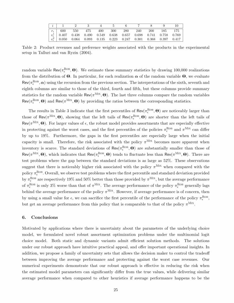
i 1 2 3 4 5 6 7 8 9 10

ri 600 550 475 400 300 280 240 200 185 175v1i 0.407 0.438 0.490 0.549 0.638 0.657 0.698 0.741 0.758 0.769v2i 0.050 0.064 0.093 0.135 0.223 0.247 0.301 0.368 0.397 0.417

Table 2: Product revenues and preference weights associated with the products in the experimentalsetup in Talluri and van Ryzin (2004).

random variable Rev(πRobϵ ,Θ). We estimate these summary statistics by drawing 100,000 realizations

from the distribution of Θ. In particular, for each realization α of the random variable Θ, we evaluate

Rev(πRobϵ ,α) using the recursion from the previous section. The interpretations of the sixth, seventh and

eighth columns are similar to those of the third, fourth and fifth, but these columns provide summary

statistics for the random variable Rev(πMix,Θ). The last three columns compare the random variables

Rev(πRobϵ ,Θ) and Rev(πMix,Θ) by providing the ratios between the corresponding statistics.

The results in Table 3 indicate that the first percentiles of Rev(πRobϵ ,Θ) are noticeably larger than

those of Rev(πMix,Θ), showing that the left tails of Rev(πRobϵ ,Θ) are shorter than the left tails of

Rev(πMix,Θ). For larger values of ϵ, the robust model provides assortments that are especially effective

in protecting against the worst cases, and the first percentiles of the policies πRobϵ and πMix can differ

by up to 19%. Furthermore, the gaps in the first percentiles are especially large when the initial

capacity is small. Therefore, the risk associated with the policy πMix becomes more apparent when

inventory is scarce. The standard deviations of Rev(πRobϵ ,Θ) are substantially smaller than those of

Rev(πMix,Θ), which indicates that Rev(πRobϵ ,Θ) tends to fluctuate less than Rev(πMix,Θ). There are

test problems where the gap between the standard deviations is as large as 52%. These observations

suggest that there is noticeably higher risk associated with the policy πMix when compared with the

policy πRobϵ . Overall, we observe test problems where the first percentile and standard deviation provided

by πRobϵ are respectively 19% and 50% better than those provided by πMix, but the average performance

of πRobϵ is only 3% worse than that of πMix. The average performance of the policy πRob

ϵ generally lags

behind the average performance of the policy πMix. However, if average performance is of concern, then

by using a small value for ϵ, we can sacrifice the first percentile of the performance of the policy πRobϵ ,

but get an average performance from this policy that is comparable to that of the policy πMix.

6. Conclusions

Motivated by applications where there is uncertainty about the parameters of the underlying choice

model, we formulated novel robust assortment optimization problems under the multinomial logit

choice model. Both static and dynamic variants admit efficient solution methods. The solutions

under our robust approach have intuitive practical appeal, and offer important operational insights. In

addition, we propose a family of uncertainty sets that allows the decision maker to control the tradeoff

between improving the average performance and protecting against the worst case revenues. Our

numerical experiments demonstrate that our robust approach is effective in reducing the risk when

the estimated model parameters can significantly differ from the true values, while delivering similar

average performance when compared to other heuristics if average performance happens to be the

25

Prob. Class Stats. for Rev(πRobϵ ,Θ) Stats. for Rev(πMix,Θ) Ratios between stats.

(C, ρ) ϵ 1 Per. Sdv. Avg. 1 Per. Sdv. Avg. 1 Per. Sdv. Avg.

(30, 0.5) 0.5 12,295 809 15,180 10,705 1,695 15,958 1.15 0.48 0.95(30, 0.5) 0.4 12,125 1,010 15,624 10,705 1,695 15,958 1.13 0.60 0.98(30, 0.5) 0.3 11,535 1,290 15,889 10,705 1,695 15,958 1.08 0.76 1.00(30, 0.5) 0.2 11,010 1,522 15,960 10,705 1,695 15,958 1.03 0.90 1.00(30, 0.5) 0.1 10,675 1,682 15,949 10,705 1,695 15,958 1.00 0.99 1.00

(30, 0.9) 0.5 11,425 1,192 14,884 9,635 2,366 15,361 1.19 0.50 0.97(30, 0.9) 0.4 11,055 1,489 15,240 9,635 2,366 15,361 1.15 0.63 0.99(30, 0.9) 0.3 10,435 1,874 15,374 9,635 2,366 15,361 1.08 0.79 1.00(30, 0.9) 0.2 9,855 2,192 15,380 9,635 2,366 15,361 1.02 0.93 1.00(30, 0.9) 0.1 9,340 2,393 15,333 9,635 2,366 15,361 0.97 1.01 1.00

(50, 0.5) 0.5 15,830 1,826 20,687 14,475 3,261 22,150 1.09 0.56 0.93(50, 0.5) 0.4 15,485 2,263 21,407 14,475 3,261 22,150 1.07 0.69 0.97(50, 0.5) 0.3 15,215 2,703 21,909 14,475 3,261 22,150 1.05 0.83 0.99(50, 0.5) 0.2 14,585 3,159 22,139 14,475 3,261 22,150 1.01 0.97 1.00(50, 0.5) 0.1 13,955 3,367 22,089 14,475 3,261 22,150 0.96 1.03 1.00

(50, 0.9) 0.5 14,855 2,425 20,343 13,295 4,256 21,639 1.12 0.57 0.94(50, 0.9) 0.4 14,445 2,983 20,987 13,295 4,256 21,639 1.09 0.70 0.97(50, 0.9) 0.3 13,935 3,600 21,422 13,295 4,256 21,639 1.05 0.85 0.99(50, 0.9) 0.2 13,485 4,154 21,608 13,295 4,256 21,639 1.01 0.98 1.00(50, 0.9) 0.1 12,795 4,382 21,539 13,295 4,256 21,639 0.96 1.03 1.00

(70, 0.5) 0.5 16,570 2,730 22,816 15,640 3,911 24,026 1.06 0.70 0.95(70, 0.5) 0.4 16,040 3,345 23,698 15,640 3,911 24,026 1.03 0.86 0.99(70, 0.5) 0.3 15,990 3,506 23,836 15,640 3,911 24,026 1.02 0.90 0.99(70, 0.5) 0.2 15,905 3,837 24,014 15,640 3,911 24,026 1.02 0.98 1.00(70, 0.5) 0.1 14,890 4,113 23,914 15,640 3,911 24,026 0.95 1.05 1.00

(70, 0.9) 0.5 15,740 3,558 22,590 14,515 5,183 23,913 1.08 0.69 0.94(70, 0.9) 0.4 14,910 4,373 23,392 14,515 5,183 23,913 1.03 0.84 0.98(70, 0.9) 0.3 14,780 4,635 23,611 14,515 5,183 23,913 1.02 0.89 0.99(70, 0.9) 0.2 14,505 5,112 23,918 14,515 5,183 23,913 1.00 0.99 1.00(70, 0.9) 0.1 13,715 5,492 23,711 14,515 5,183 23,913 0.94 1.06 0.99

(90, 0.5) 0.5 16,595 2,950 22,917 16,000 3,716 23,999 1.04 0.79 0.95(90, 0.5) 0.4 16,000 3,714 24,000 16,000 3,716 23,999 1.00 1.00 1.00(90, 0.5) 0.3 15,985 3,716 23,999 16,000 3,716 23,999 1.00 1.00 1.00(90, 0.5) 0.2 16,000 3,716 23,999 16,000 3,716 23,999 1.00 1.00 1.00(90, 0.5) 0.1 15,025 4,239 24,001 16,000 3,716 23,999 0.94 1.14 1.00

(90, 0.9) 0.5 15,575 3,944 22,870 14,865 5,049 23,949 1.05 0.78 0.95(90, 0.9) 0.4 14,865 5,048 23,948 14,865 5,049 23,949 1.00 1.00 1.00(90, 0.9) 0.3 14,865 5,048 23,948 14,865 5,049 23,949 1.00 1.00 1.00(90, 0.9) 0.2 14,865 5,049 23,948 14,865 5,049 23,949 1.00 1.00 1.00(90, 0.9) 0.1 13,650 5,817 23,942 14,865 5,049 23,949 0.92 1.15 1.00

Table 3: Comparison between the total expected revenues obtained by the policies πRobϵ and πMix.

26

performance measure of interest.

In this paper, we assumed that the model parameters lie in an uncertainty set, but we do not refine

the uncertainty set as we observe the purchases of the customers. This is a reasonable assumption when it

is difficult to learn the model parameters either because there are a few sale opportunities or the different

customers are so distinct from each other that the purchase behavior of one customer tells us little about

the purchase behavior of others. Another option is to resolve the problem as more information becomes

available and the uncertainty sets are refined. Nevertheless, there are undoubtedly settings where one

could learn from the purchase behavior of the past customers to predict the preferences of the future

customers. In this case, adaptively refining the offered assortment and the uncertainty set by embedding

a learning mechanism into the assortment optimization model would be beneficial.

It would also be worthwhile to compare the solution under our robust formulation to the one obtained

by putting a prior distribution on the likely values of the model parameters. Understanding the tradeoffs

between these two approaches might lead to a new framework for thinking about assortment optimization

problems. Finally, it would be interesting to extend our analysis to more complex choice models.

Acknowledgement

The authors would like to thank the Associate Editor and the two referees for their thoughtful and

detailed comments. Their suggestions led us to consider a robust dynamic capacity allocation model in

Section 4, and greatly improved the presentation of the paper. We also want to thank Guillermo Gallego

and Assaf Zeevi for their helpful suggestions and discussions during the presentation of this work at the

INFORMS Revenue Management and Pricing Conference, and Adrian Lewis for helpful discussions on

linear-fractional functions. The research of the first and second authors was supported in part by the

National Science Foundation through grants DMS-0732196, CMMI-0855928, CMMI-0746844, CMMI-

0969113, and CMMI-0825004.

References

Anderson, S., A. de Palma, and J. F. Thisse. 1992. Discrete choice theory of product differentiation.Cambridge, MA: MIT Press.

Ben-Akiva, M., and S. Lerman. 1985. Discrete choice analysis: Theory and application to travel demand.Cambridge, MA: MIT Press.

Ben-Tal, A., and A. Nemirovski. 1999. Robust solutions of uncertain linear programs. OperationsResearch Letters 25 (1): 1–13.

Bertsimas, D., D. Pachamanovab, and M. Sim. 2004. Robust linear optimization under general norms.Operations Research Letters 32 (6): 510–516.

Bertsimas, D., and M. Sim. 2003. Robust discrete optimization and network flows. MathematicalProgramming 98 (1): 49–71.

Bertsimas, D., and M. Sim. 2004. The price of robustness. Operations Research 52 (1): 35–53.

Birbil, S. I., J. B. G. Frank, J. A. S. Gromicho, and S. Zhang. 2009. The role of robust optimization insingle-leg airline revenue management. Management Science 55:148–163.

27

Boyd, S., and L. Vandenberghe. 2004. Convex optimization. Cambridge, UK: Cambridge UniversityPress.

Bront, J. M., I. Mendez Diaz, and G. Vulcano. 2009. A column generation algorithm for choice-basednetwork revenue management. Operations Research 57 (3): 769–784.

Chaneton, J., and G. Vulcano. 2011. Computing bid-prices for revenue management under customerchoice behavior. To appear in Manufacturing and Service Operations Management.

Farias, V. F., S. Jagabathula, and D. Shah. 2010. A non-parametric approach to modeling choice withlimited data. Working paper, MIT.

Gallego, G., G. Iyengar, R. Phillips, and A. Dubey. 2004. Managing flexible products on a network.Working Paper, Columbia University.

Iyengar, G. N. 2005. Robust dynamic programming. Mathematics of Operations Research 30 (2):257–280.

Kok, A. G., M. Fisher, and R. Vaidyanathan. 2008. Assortment planning: Review of literature andindustry practice. In Retail Supply Chain Management: Springer.

Kunnumkal, S., and H. Topaloglu. 2008. A refined deterministic linear program for the network revenuemanagement problem with customer choice behavior. Naval Research Logistics 55 (6): 563–580.

Kunnumkal, S., and H. Topaloglu. 2010. A New Dynamic Programming Decomposition Method for theNetwork Revenue Management Problem with Customer Choice Behavior. Production and OperationsManagement 19 (5): 575–590.

Liu, Q., and G. J. van Ryzin. 2008. On the choice-based linear programming model for network revenuemanagement. Manufacturing and Service Operations Management 10 (2): 288–310.

Liu, Q., and G. J. van Ryzin. 2008. Strategic capacity rationing to induce early purchases. ManagementScience 54 (6): 1115–1131.

Megiddo, N. 1979. Combinatorial optimization with rational objective functions. Mathematics ofOperations Research 4 (4): 414–424.

Meissner, J., and A. K. Strauss. 2010. Improved bid prices for choice-based network revenuemanagement. Working paper, Department of Management Science, Lancaster University.

Meissner, J., and A. K. Strauss. 2011. Network revenue management with inventory-sensitive bid pricesand customer choice. To appear in European Journal of Operational Research.

Mendez-Diaz, I., J. M. Bront, G. Vulcano, and P. Zabala. 2010. A Branch-and-Cut Algorithm for theLatent-Class Logit Assortment Problem. Working Paper, New York University.

Perakis, G., and G. Roels. 2010. Robust controls for network revenue management. Manufacturing &Service Operations Management 12:56–76.

Phillips, R. 2011. Efficient frontiers in revenue management. INFORMS Revenue Management andPricing Section Conference, New York, NY.

Rusmevichientong, P., Z.-J. M. Shen, and D. B. Shmoys. 2010. Dynamic assortment optimization witha multinomial logit choice model and capacity constraint. Operations Research 58 (6): 1666–1680.

Rusmevichientong, P., D. B. Shmoys, and H. Topaloglu. 2010. Assortment optimization with mixturesof logits. Working paper, Cornell University.

Ruszczynski, A. 2006. Nonlinear optimization. Princeton, New Jersey: Princeton University Press.

Su, X. 2007. Intertemporal pricing with strategic customer behavior. Management Science 53 (5):726–741.

Su, X. 2010. Intertemporal pricing and consumer stockpiling. Operations Research 58 (4): 1133–1147.

28

Talluri, K. 2010. A randomized concave programming method for choice network revenue management.Working paper, Universitat Pompeu Fabra, Barcelona, Spain.

Talluri, K., and G. J. van Ryzin. 2004. Revenue management under a general discrete choice model ofconsumer behavior. Management Science 50 (1): 15–33.

van Ryzin, G. J., and S. Mahajan. 1999. On the relationship between inventory costs and varietybenefits in retail assortments. Management Science 45:1496–1509.

van Ryzin, G. J., and G. Vulcano. 2008. Computing virtual nesting controls for network revenuemanagement under customer choice behavior. Manufacturing and Service Operations Management 10(3): 448–467.

Vulcano, G., G. J. van Ryzin, and W. Chaar. 2010. Choice-based revenue management: An empiricalstudy of estimation and optimization. Manufacturing and Service Operations Management 12 (3):371–392.

Vulcano, G., G. J. van Ryzin, and R. Ratliff. 2011. Estimating primary demand for substitutableproducts from sales transaction data. To appear in Operations Research.

Zhang, D. 2011. An improved dynamic programming decomposition approach for network revenuemanagement. Manufacturing and Service Operations Management 13 (1): 35–52.

Zhang, D., and D. Adelman. 2009, August. An approximate dynamic programming approach to networkrevenue management with customer choice. Transportation Science 43 (3): 381–394.

29

A. Appendix: Proof of Theorem 4.1

We first establish, by induction, that the value functions are concave in the remaining capacity; that is,

∆Jt(x) is decreasing in x for all t. The result is trivially true for ∆JT+1(·). So, assume that it holds

for ∆Jt+1(·). We will now prove that it also holds for ∆Jt(·). It follows from the Bellman equation in

the Dynamic Robust problem and the definition of S∗t (x) that

∆Jt(x+ 2)−∆Jt(x+ 1) = Jt(x+ 2)− Jt(x+ 1)− Jt(x+ 1) + Jt(x)

= maxSt⊆A

minvt∈Vt

{∑i∈St

ϕi(St,vt) (ri −∆Jt+1(x+ 2))

}+ Jt+1(x+ 2)

− maxSt⊆A

minvt∈Vt

{∑i∈St


}− Jt+1(x+ 1)

− maxSt⊆A

minvt∈Vt

{∑i∈St


}− Jt+1(x+ 1)

+ maxSt⊆A

minvt∈Vt

{∑i∈St


}+ Jt+1(x)

= ∆Jt+1(x+ 2)−∆Jt+1(x+ 1) + minvt∈Vt

∑i∈S∗

t (x+2)

ϕi(S∗t (x+ 2),vt) (ri −∆Jt+1(x+ 2))

− min

vt∈Vt

∑i∈S∗

t (x+1)

ϕi(S∗t (x+ 1),vt) (ri −∆Jt+1(x+ 1))

+ min

vt∈Vt

∑i∈S∗

t (x)

ϕi(S∗t (x),vt) (ri −∆Jt+1(x))

− min

vt∈Vt

∑i∈S∗

t (x+1)

ϕi(S∗t (x+ 1),vt) (ri −∆Jt+1(x+ 1))

.

We will now bound the terms in the right hand side of the above equality. By definition, S∗t (x + 1) is

the optimal solution to the problem maxSt⊆{1,2,...,n}minvt∈Vt

∑i∈St

ϕi(St,vt) (ri −∆Jt+1(x+ 1)), which

implies that

minvt∈Vt

∑i∈S∗

t (x+1)

ϕi(S∗t (x+ 1),vt) (ri −∆Jt+1(x+ 1))

≥ minvt∈Vt

∑i∈S∗

t (x)

ϕi(S∗t (x),vt) (ri −∆Jt+1(x+ 1))

= min

vt∈Vt

∑i∈S∗

t (x)

ϕi(S∗t (x),vt) (ri −∆Jt+1(x)) +

∑i∈S∗

t (x)

ϕi(S∗t (x),vt) (∆Jt+1(x)−∆Jt+1(x+ 1))

≥ min

vt∈Vt

∑i∈S∗

t (x)


+

minvt∈Vt

∑i∈S∗

t (x)

ϕi(S∗t (x),vt)

(∆Jt+1(x)−∆Jt+1(x+ 1)) ,

30

where the last inequality follows from our hypothesis that ∆Jt+1(x)−∆Jt+1(x+ 1) ≥ 0. Therefore,

minvt∈Vt

∑i∈S∗

t (x)


− minvt∈Vt

∑i∈S∗

t (x+1)

ϕi(S∗t (x+ 1),vt) (ri −∆Jt+1(x+ 1))

≤

minvt∈Vt

∑i∈S∗

t (x)

ϕi(S∗t (x),vt)

(∆Jt+1(x+ 1)−∆Jt+1(x)) .

Using a similar argument, we have that

minvt∈Vt

∑i∈S∗

t (x+1)

ϕi(S∗t (x+ 1),vt) (ri −∆Jt+1(x+ 1))

≥ min

vt∈Vt

∑i∈S∗

t (x+2)

ϕi(S∗t (x+ 2),vt) (ri −∆Jt+1(x+ 1))

= min

vt∈Vt

∑i∈S∗

t (x+2)

ϕi(S∗t (x+ 2),vt) (ri −∆Jt+1(x+ 2))

+∑

i∈S∗t (x+2)

ϕi(S∗t (x+ 2),vt) (∆Jt+1(x+ 2)−∆Jt+1(x+ 1))

≥ min

vt∈Vt

∑i∈S∗

t (x+2)

ϕi(S∗t (x+ 2),vt) (ri −∆Jt+1(x+ 2))

+

maxvt∈Vt

∑i∈S∗

t (x+2)

ϕi(S∗t (x+ 2),vt)

(∆Jt+1(x+ 2)−∆Jt+1(x+ 1)) ,

where the last inequality follows from the fact that ∆Jt+1(x+2)−∆Jt+1(x+1) ≤ 0, which means that

minvt∈Vt

∑i∈S∗

t (x+2)

ϕi(S∗t (x+ 2),vt) (∆Jt+1(x+ 2)−∆Jt+1(x+ 1))

=

maxvt∈Vt

∑i∈S∗

t (x+2)


(∆Jt+1(x+ 2)−∆Jt+1(x+ 1)) .

Therefore, we have

minvt∈Vt

∑i∈S∗

t (x+2)

ϕi(S∗t (x+ 2),vt) (ri −∆Jt+1(x+ 2))

− min

vt∈Vt

∑i∈S∗

t (x+1)

ϕi(S∗t (x+ 1),vt) (ri −∆Jt+1(x+ 1))

≤ −

maxvt∈Vt

∑i∈S∗

t (x+2)


(∆Jt+1(x+ 2)−∆Jt+1(x+ 1)) .

31

Putting everything together, we bound ∆Jt(x+ 2)−∆Jt(x+ 1) by

∆Jt(x+ 2)−∆Jt(x+ 1)

≤ ∆Jt+1(x+ 2)−∆Jt+1(x+ 1)−

maxvt∈Vt

∑i∈S∗

t (x+2)


(∆Jt+1(x+ 2)−∆Jt+1(x+ 1))

+

minvt∈Vt

∑i∈S∗

t (x)

ϕi(S∗t (x),vt)

(∆Jt+1(x+ 1)−∆Jt+1(x))

=

1− maxvt∈Vt

∑i∈S∗

t (x+2)


(∆Jt+1(x+ 2)−∆Jt+1(x+ 1))

+

minvt∈Vt

∑i∈S∗

t (x)

ϕi(S∗t (x),vt)

(∆Jt+1(x+ 1)−∆Jt+1(x))

≤ 0 ,

where the last inequality follows from the fact that maxvt∈Vt

∑i∈St

ϕi(S∗t (x+ 2),vt) ≤ 1 and from our

inductive hypothesis that ∆Jt+1(x + 2) − ∆Jt+1(x + 1) ≤ 0 and ∆Jt+1(x + 1) − ∆Jt+1(x) ≤ 0. This

completes the induction.

We will now use the concavity of the value functions to show that marginal value of capacity is

decreasing with time; that is, ∆Jt+1(x+ 1) ≤ ∆Jt(x+ 1). It follows from the Bellman equation in the

Dynamic Robust problem that

∆Jt(x+ 1)−∆Jt+1(x+ 1)

= Jt(x+ 1)− Jt(x)−∆Jt+1(x+ 1)

= maxSt

minvt∈Vt

{∑i∈St


}−max

St

minvt∈Vt

{∑i∈St


}

= minvt∈Vt

∑i∈S∗

t (x+1)

ϕi(S∗t (x+ 1),vt) (ri −∆Jt+1(x+ 1))

− minvt∈Vt

∑i∈S∗

t (x)


≥ min

vt∈Vt

∑i∈S∗

t (x+1)

ϕi(S∗t (x+ 1),vt) (ri −∆Jt+1(x+ 1))

− minvt∈Vt

∑i∈S∗

t (x)

ϕi(S∗t (x),vt) (ri −∆Jt+1(x+ 1))

≥ 0 ,

where the first inequality follows from the fact that ∆Jt+1(x) ≥ ∆Jt+1(x+1) and the second inequality

follows from the definition S∗t (x+ 1).

B. Appendix: Generation of Test Problems

To come up with the preference weights for each customer type, we sample the parameter σi from the

uniform distribution over [0, 1] for each product i. A large value for σi indicates that product i is a

specialty product and the preference weights associated with product i show large variability among the

32

different customer types. On the other hand, a small value for σi indicates that product i is a staple

product and the preference weights associated with product i does not show large variability among

the different customer types. In this case, we sample the parameter ϑgi from the uniform distribution

over [0, 10] for each product i and customer type g, and set vgi = (1 − σi)ϑgi /n with probability 1/2

and vgi = (1 + σi)ϑgi /n with probability 1/2. To see the motivation behind our choice of the preference

weights, we observe that if σi is close to zero, then vgi is close to ϑgi /n. On the other hand, if σi is close

to one, then vgi is either close to zero or close to 2ϑgi . Therefore, as we mention above, the parameter σi

is a measure of the variability of the preference weights associated with product i among the different

customer types. For the no purchase weights, we set vg0 = 1 for each customer type g. We observe

that the expectation of vgi is 5/n. If vgi takes a value close to its expectation and we offer all products

to our customers, then the probability that a customer leaves without purchasing anything is given by

1/[1 +∑n

i=1 5/n] = 1/6. Therefore, we expect to have a significant probability that a customer leaves

without purchasing anything even if we offer all products to our customers.

To come up with the revenues of the products, we sample κi from the uniform distribution over

[0, 200] and set ri = [n+1− i]κi. In this way, we hope to generate a set of products with a large variety

in revenues. After generating the revenues of all of the products, we renumber the products to make

sure that r1 ≥ r2 ≥ · · · ≥ rn.

33

Documents

Robust Assortment Optimization in Revenue Management … · maintain comparable average revenue if average revenue is the performance measure of interest. 1. Introduction A traditional