Embed Size (px)
Citation preview
Robotic Data Mules for Collecting Data over Sparse
Sensor Fields∗
Deepak Bhadauria
Computer Science and Engineering
University of Minnesota
Minneapolis, MN 55455
Onur Tekdas
Computer Science and Engineering
University of Minnesota
Minneapolis, MN 55455
Volkan Isler
Computer Science and Engineering
University of Minnesota
Minneapolis, MN 55455
Abstract
We present a robotic system for collecting data from wireless devices dispersed across a large
environment. In such applications, deploying a network of stationary wireless sensors may
be infeasible because many relay nodes must be deployed to ensure connectivity. Instead,
our system utilizes robots which act as data mules and gather the data from wireless sensor
network nodes.
We address the problem of planning paths of multiple robots so as to collect the data from
all sensors in the least amount of time. In this new routing problem, which we call the Data
Gathering Problem (DGP), the total download time depends on not only the robots’ travel
time but also the time to download data from a sensor, and the number of sensors assigned
to the robot.
We start with a special case of DGP where the robots’ motion is restricted to a curve which
contains the base station at one end. For this version, we present an optimal algorithm.
∗A preliminary version of this paper appeared in IROS’09 (Bhadauria and Isler, 2009).

Next, we study the 2D version, and present a constant factor approximation algorithm for
DGP on the plane. Finally, we present field experiments in which an autonomous robotic
data mule collects data from the nodes of a wireless sensor network deployed over a large
field.
1 Introduction
In the last decade, Wireless Sensor Networks (WSNs) have been utilized in numerous sensing automation
tasks such as humidity and temperature monitoring and surveillance. In these applications, sensing devices
equipped with communication and computation capabilities collect data, and form a network to relay it back
to a gateway. When the area to be covered is large and the sensing locations are far, this approach requires
deploying many relay nodes to form a connected network. In the early days of WSN research this issue
was overlooked because the researchers envisioned that the cost of the network nodes would be minimal.
Further, it was expected that tiny and long-lasting batteries would be available for long term operation.
However, sensor nodes are still costly (a basic device runs on AA batteries and costs around $100). In
parallel, maintaining the network (e.g. replacing batteries) requires manual labor which adds significantly
to the operation costs. Therefore, traditional WSN approach of deploying stationary nodes is not scalable
in applications where a large area must be covered with a sparse deployment. A typical example is habitat
monitoring where soil humidity and temperature at areas visited by a particular species is collected.
In our recent work, we presented an alternative to static relay-nodes for such applications: using robots as
data mules to collect the data from sensors (Tekdas et al., 2009). This approach has a number of advantages
over deploying a dense static network. First of all, since relay nodes are no longer needed, operational costs
are minimized. Second, the lifetime of the network is maximized because the robots can get close to the
sensor nodes to download the data. In addition to reducing the energy consumption during transmission (less
power is needed), proximity also reduces the data loss rate, which results in smaller number of transmissions
per byte. Thus, hybrid networks consisting mobile robots with communication capabilities in addition
to stationary WSN nodes can be useful in addressing the scalability issue in some large-scale monitoring
applications.
A crucial problem that arises in data muling applications is the problem of planning the routes of robotic
mules: given locations of n sensors, compute the routes of k robots so that the time to download the data
from all sensors is minimized. In this paper, we study this path planning problem which we refer to as the
Data Gathering Problem (DGP). Note that in DGP, the cost incurred by a robot depends on not only the
robot’s travel time but also the time to download data from a sensor, and the number of sensors assigned to
the robot.
The well-known Traveling Salesperson Problem (TSP) asks for the shortest path for a salesperson to visit n
cities (Applegate et al., 2006). There is a variant of TSP, called k-TSP, where k travelers visit n cities, and
the objective is to minimize the length of the maximum tour (Frederickson et al., 1978). Even though DGP
resembles k-TSP, a closer look reveals important differences.
B
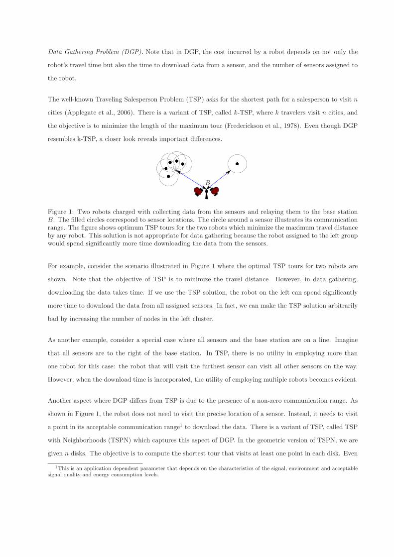
Figure 1: Two robots charged with collecting data from the sensors and relaying them to the base stationB. The filled circles correspond to sensor locations. The circle around a sensor illustrates its communicationrange. The figure shows optimum TSP tours for the two robots which minimize the maximum travel distanceby any robot. This solution is not appropriate for data gathering because the robot assigned to the left groupwould spend significantly more time downloading the data from the sensors.
For example, consider the scenario illustrated in Figure 1 where the optimal TSP tours for two robots are
shown. Note that the objective of TSP is to minimize the travel distance. However, in data gathering,
downloading the data takes time. If we use the TSP solution, the robot on the left can spend significantly
more time to download the data from all assigned sensors. In fact, we can make the TSP solution arbitrarily
bad by increasing the number of nodes in the left cluster.
As another example, consider a special case where all sensors and the base station are on a line. Imagine
that all sensors are to the right of the base station. In TSP, there is no utility in employing more than
one robot for this case: the robot that will visit the furthest sensor can visit all other sensors on the way.
However, when the download time is incorporated, the utility of employing multiple robots becomes evident.
Another aspect where DGP differs from TSP is due to the presence of a non-zero communication range. As
shown in Figure 1, the robot does not need to visit the precise location of a sensor. Instead, it needs to visit
a point in its acceptable communication range1 to download the data. There is a variant of TSP, called TSP
with Neighborhoods (TSPN) which captures this aspect of DGP. In the geometric version of TSPN, we are
given n disks. The objective is to compute the shortest tour that visits at least one point in each disk. Even
1This is an application dependent parameter that depends on the characteristics of the signal, environment and acceptablesignal quality and energy consumption levels.

though efficient algorithms for TSPN exist (Dumitrescu and Mitchell, 2003; Mitchell, 2007), there are no
algorithms for k-TSPN where the objective is to compute TSPN tours for k robots.
Our results and organization of the paper: In Section 3, we formalize the Data Gathering Problem. Next, in
Section 4.1, we present an optimal algorithm for the 1D version where the robots are restricted to move along
a curve. For the 2D case, we make two theoretical contributions: (i) we give a constant factor approximation
algorithm for 2D version of the problem in Section 4.2, (ii) for sparse deployments where the utility of
using robots is significant, we give a heuristic which improves on the performance of the first algorithm
(Section 4.3). We present an opportunistic algorithm in Section 5 to improve the efficiency of our system
in the presence of navigational uncertainties. Utility of the algorithms is demonstrated in simulations in
Section 6. We make another contribution in this paper by presenting the design and implementation of a
data muling system which uses the proposed algorithm for data collection. Details of this system and the
results of the field experiments are reported in Section 7. In the next section, we start with a brief overview
of the related work.
2 Related Work
In recent years, using mobility for carrying data in ad-hoc networks has received significant attention.
However, most of the existing literature focuses on settings where the mobility of the network entities is
not controlled. The use of controllable entities (such as robots with wireless communication capabilities)
for data muling has been receiving increasing attention. In this section, we present an overview of related
work on data muling followed by an overview of relevant work on the Traveling Salesperson Problem and its
variants.
(Shah et al., 2003) present a data muling system which uses uncontrolled entities (such as animals, humans
with wireless devices) for carrying data. The authors present a three tier sensor network architecture. The
bottom layer consists of a sparse sensor network. In the middle layer there are mobile entities such as vehicles
and humans which carry the data from bottom layer to the access points in the top level. These ideas were
also implemented in real systems in ZebraNet (Juang et al., 2002) and Smart-tag (Beaufour et al., 2002)
projects.
In the next set of results, the mobile agent is still uncontrolled however the mobility model knowledge is
used to optimize the various parameters of the network. In (Chakrabarti et al., 2003), the authors explore
the use of observed mobile agents in reducing the energy consumption in sensor networks. In (Jea et al.,
2005), data mules’ trajectories are parallel line segments and the goal is to find the balanced assignment of
sensors so that the tour times of data mules is minimized. In (Boloni and Turgut, 2008), the authors explore
the transmission scheduling i.e. schedule to wake up a node and transmit to the data mule. The solution
is presented under the assumption that the mule follows a random-waypoint mobility pattern. An adaptive
data transfer protocol which minimizes the time interval for a single sensor to offload the data is presented
in (Anastasi et al., 2007). This protocol considers the packet loss rate due to the distance between sensor
and the data mule at the time of offload. A simple protocol is presented in (Anastasi et al., 2008) in which
nodes send periodic beacons with low duty cycle and turns on their radio when the connection with a data
mule is satisfied. A recent review on the state of the art in exploiting sink mobility can be found in (Ma
et al., 2008; Ekici et al., 2006; Gu et al., 2005; Xing et al., 2005)
The study of systems which use controllable agents as data mules is relatively recent. A variant of the Data
Gathering Problem (DGP) was considered as a scheduling problem in (Kansal et al., 2004). The authors
consider the control of the robot’s velocity along a fixed path to improve transmission quality. They do not
address the computation of the path. Similarly (Sugihara and Gupta, 2010) study the speed control problem
for the data mule when it is downloading data from a sensor while traveling within its communication
range. Authors present a heuristic which computes the speed change along the mule’s path and a schedule
for downloading the data from the sensors. DGP is also considered as a coverage problem. In (Gasparri
et al., 2008), the authors aim to find a path for each robot such that all paths are disjoint, all sensors
are covered and all paths are of equal length. They investigate the performance of their algorithms in
simulation. In (Williams and Burdick, 2006), the authors present a heuristic for the multi-robot boundary
coverage problem. In a boundary coverage problem we are given k robots and n convex, two-dimensional
objects. The goal is to find a tour for each robot such that all points on the boundary of each object are
inspected and the inspection load is balanced. None of these algorithms present any theoretical guarantees
on the performance of the paths.
In the following body of work, variants of DGP are formulated as TSP instances. In (Tirta et al., 2004),
the authors present heuristics to schedule visits of a mobile agent to collect data from cluster heads. The
heuristics focus on data latency and data aggregation rate of clusters. In our work we focus on the travel
time of the mobile agents and present algorithms with theoretical performance guarantees. (Wu et al., 2009)
present a heuristic approach for minimizing path length in data muling. Authors consider spatially separated
WSNs which are to be connected by a data mule. The objective is to find a path for mule which visits one
sensor each in each WSN. Their heuristic creates a path from the convex hull of the set of sensors, choosing
one sensor from each WSN, and modifies the path to add the sensors from WSNs not covered by the convex
hull. In (Yuan et al., 2007), the authors formulate the problem of collecting sensor data using a single robot
as an instance of the TSP with neighborhoods (TSPN) problem. They do not address the time spent in
downloading data. As shown in Figure 1, ignoring transmission time can worsen the performance of the
system drastically. None of the work that uses TSP-based heuristics has been implemented and tested on a
real system.
Implementations of data mule system are presented in (Dunbabin et al., 2006; Tekdas et al., 2009). In (Dun-
babin et al., 2006), the authors present an underwater data muling system. In the underwater scenario, sen-
sors and underwater vehicles communicate through optical communication, which requires a close proximity
as well as a good view-angle to start communication. The authors use a TSP algorithm to compute the
trajectory of the robot. However since GPS localization is not available under the water, the vehicle has to
navigate under high uncertainty and periodically surface to get GPS fix. This makes the designing global
routing algorithms challenging. The authors propose spiral movement for the robot to find the sensors.
This strategy is not efficient for our scenario, in which the sensor locations are known and the robot can
localize itself. In our previous work (Tekdas et al., 2009), we implemented a system which uses TSP and
k-TSP algorithms to find efficient strategies for multiple data mules. However we did not incorporate the
communication range of the sensors as well as the download times which are the main contributions of this
paper.
The Traveling Salesperson Problem is a fundamental combinatorial optimization problem. It has been studied
to the extent that there are books dedicated to it (Applegate et al., 2006). The work presented in this paper
builds on algorithms for two variants of TSP: The geometric version of TSP with Neighborhoods (Dumitrescu
and Mitchell, 2003), and k-TSP (Frederickson et al., 1978). We present an overview of these algorithms in
Section 4.2.
3 The Data Gathering Problem
In this section we define the data gathering problem and present assumptions regarding the system.
The input consists of the coordinates of n sensors and a base station b. Each of the k robots is charged with
downloading data from sensors assigned to it and uploading it to the base station. We define the coverage

of a sensor as transferring the sensor’s data to the base station by a data mule.
We make the following assumptions:
• The sensors are identical. The amount of data to be downloaded from each sensor is the same.
Further, the transmission ranges and data sending rates of all the sensors are identical. We assume
that each sensor can sense data and transmit it up to a distance Tr units with uniform data rate.
Therefore, the time required to download data from every sensor, Td, is identical. We also assume
that transmission ranges of all the sensors are obstacle free and a robot can access any point in these
transmission ranges.
• The data is downloaded by k identical robots which have wireless communication capabilities and
can travel at a constant speed of ν. In this work, we do not consider higher order constraints
such as acceleration. Also, without loss of generality, we will use ν = 1. The robots have infinite
buffer capacities (since they can carry large storage devices). Similarly, we do not consider energy
limitations for robots. We assume that the robots can localize themselves and navigate in the
environment. We assume that the communication disk of each sensor is free of obstacles (so that
the robot can traverse the boundary of each disk). The robots stop to download data.
We present algorithms for DGP in the succeeding sections under these assumptions, and validate them in
field experiments later on.
4 Algorithms for DGP
4.1 The 1D Data Gathering Problem
In this section, we study the 1D version of the DGP where the robots are restricted to move along a curve
X. This case has practical applications in scenarios where robots move along a rail-line, or there is a single
path they can move along in a rough terrain.
We assume that base station is at one end point of the curve X; i.e. at x = 0 where x is the parametrization
of the underlying curve.
For each sensor s, compute the intersection of the communication disk (centered at s with radius Tr) with
the curve X. Among all the points of the intersection, let xs be the point closest to base station. We will

B
X
xs
sTr
Figure 2: A 1D instance of the DGP. Robots can travel only on curve X. xs represents the download locationof sensor s. To download data from s, a robot has to stop at xs.
choose xs as the download location of s. Since all intersections are assumed to be on one side of the base
station, any robot which will download data from s can do so from location xs without incurring additional
travel costs. Hereafter, we represent each sensor with its download location. For this version of the problem
where xs > 0 for all s, we will present an optimal algorithm for gathering data with k robots.
Let U be the set of robots. Now consider a solution to the 1D DGP. For any two robots u, v ∈ U , let
S(u) = {u1, u2, . . . , uk} and S(v) = {v1, v2, . . . , vl} be the sets of sensors assigned to u and v respectively in
the solution (we overload the notation and use ui to refer both a sensor and its download location). S(u)
and S(v) are ordered and labeled such that u1 ≤ u2 ≤ . . . ≤ uk and v1 ≤ v2 ≤ . . . ≤ vl. While ordering
download locations, we break ties arbitrarily. We say that S(u) and S(v) are non-overlapping if uk ≤ v1 or
vl ≤ u1 .
The following lemma sheds light onto the structure of the optimal data collection.
Lemma 1. There exists an optimal solution to cover n sensors with k robots in which ∀u, v ∈ U , S(u) and
S(v) are non-overlapping.
Proof. Among all optimal solutions, consider the optimal solution OPT with the largest number of non-
overlapping pairs of robots. We claim that there is no overlapping pair in OPT. Suppose, to the contrary,
that there is a pair of robots whose sensors are overlapping. We consider two cases. It the first case, there
exist two nodes u, v ∈ U such that S(u) and S(v) are overlapping partially (Figure 3 (a)). If this not the
case, then the overlap must be a complete overlap (Figure 3 (b)). We show that in both cases, the overlap
can be removed without introducing additional overlaps. This will contradict with the minimality of the
number of overlapping pairs in OPT. Without loss of generality, we can assume that u1 ≤ v1.
Case (a): There is a partial overlap of S(u) and S(v). Let the time to cover S(u) (resp. S(v)) by robot u
(resp. v) be T (u) (resp. T (v)). Then

T (u) = 2uk + kTd and T (v) = 2vl + lTd.
In this case, we can reassign sensor uk ∈ S(u) to robot v and sensor v1 ∈ S(v) to robot u. This will give us
new sets of sensors S′(u) = S(u)−{uk}+ {v1} and S′(v) = S(v)−{v1}+ {uk} that are assigned to u and v.
Let u′k ∈ S′(u) be the sensor which is farthest from the base station. Then the new coverage times will be:
T ′(u) = 2u′k + kTd and T ′(v) = 2vl + lTd
Since u′k ≤ uk, we have T ′(u) ≤ T (u). Also T ′(v) = T (v). This reassignment operation does not increase the
coverage cost of any of the two robots. We can continue reassigning in the similar way until u′k ≤ v1. This
gives us a new assignment for the robots u and v where u′k ≤ v1, or S′(u) and S′(v) are non-overlapping.
Note that, since the segments are only getting smaller, no additional overlaps are introduced. Therefore, we
reduced the number of overlaps in OPT by one which contradicts the minimality of OPT in terms of the
number of non-overlapping pairs.
Case (b): There are no partial overlaps (that is, case (a) is not true). In this case, there must be two sensors
u and v such that S(u) completely overlaps S(v) (Figure 3(b)). Among all the segments (sensors assigned
to a single robot) contained in S(u), let S(v) be the one with the leftmost left-end.
We can reassign sensor u1 ∈ S(u) to robot v and sensor v1 ∈ S(v) to robot u. This does not increase the cost
of coverage for any of the robots u and v. Note that this operation does not increase the number of overlaps
because there are no partial overlaps and v is the leftmost among all segments contained in u. After this
reassignment, this case becomes similar to case (a). Using the same argument, this means that the number
of overlaps can be reduced – a contradiction.
(a)
(b)
... ...
...
...
......u1
u1
uk
uk
v1
v1
vl
vl
Figure 3: Two primary ways in which S(u) and S(v) can be overlapping: (a) partial overlap (b) completeoverlap.
Lemma 1 sheds light on the structure of sensor assignments in an optimal solution. We now present a
dynamic programming algorithm to exploit this structure and to gather the data from n sensors using k

robots in an optimal fashion.
Let’s order and label sensors from s1 to sn with increasing distance of their download locations from the
base station (again, si refers to both the ith sensor and its download location). Let cost(m, l) be the cost to
cover sensors sm to sl, m ≤ l by a robot. Therefore cost(m, l) = 2sl + (l −m + 1)Td. We create an n × k
table T . Each entry T [i, j] represents the optimal cost to cover s1 to si sensors by j robots. The entries of
the table are computed using the following recurrence equation:
T [i, j] =
T [i, i] if j > i
2si + iTd if j = 1
min1≤m<i
(T [m, j − 1] + cost(m + 1, i)) otherwise
(1)
Lemma 2. When all entries are computed, T [i, j] stores the optimal coverage time for the first i sensors
using j mules.
Proof. We prove the lemma by induction on j, the number of robots.
Basis: For j = 1 the minimum time to cover s1 to si, T [i, 1] = 2si + iTd ∀i ∈ {1, n}. This is minimum
because to cover i sensors any robot has to travel up to download location of farthest sensor and download
data from all the sensors.
Inductive hypothesis: Let T [l, j − 1] be minimum time required to cover first l sensors using j − 1 robots
∀l ∈ {1, n}. Now for j robots T [l, j] = min1≤m<l
(T [m, j − 1] + cost(m + 1, l)). Since T [m, j−1] is the minimum
coverage time for m sensors with j − 1 robots and the value of T [l, j] is set to minimum of all l− 1 possible
values of m, T [l, j] is minimum coverage time of l sensors with j mules.
Thus, the entry T [n, k] gives us the desired solution. The running time of the algorithm can be easily seen
to be O(n2k). The main result of this section is summarized by the following theorem.
Theorem 1. There exists an optimal polynomial time algorithm to solve the 1D version of the data gathering
problem when all the sensors are on one side of the base station.
4.2 The 2D Data Gathering Problem
In 2D version of DGP, the robot is not restricted to a curve. Instead, it can take any path on the plane.
The 2D version of DGP is NP-Hard because it contains the Euclidean TSP problem as a special case. To
see this, take a DGP instance where the number of robots is 1, the download time is an arbitrary constant
and the transmission range is 0. In this instance minimizing the tour time is equivalent to minimizing the
tour length, and the tour visits each sensor point. It is equivalent to a Euclidean TSP instance which is
NP-Hard.
In this section, we present an approximation algorithm for 2D DGP. Our algorithm uses tools and techniques
developed for the following variants of TSP: TSP with neighborhoods (TSPN) and k-TSP. After an overview
of these two algorithms, we show how they can be combined to obtain a constant factor approximation
algorithm for the 2D DGP problem.
(Dumitrescu and Mitchell, 2003) present a constant factor algorithm for TSPN where the neighborhoods
are disks of unit radius. The approximation ratio of this algorithm is 11.15. In this work, we refer to this
algorithm by TspnTour. TspnTour first computes a maximal independent set, say I, of non-intersecting
disks from the given set of disks. Next a TSP tour, τI , of centers of all the disks in I is computed. A TSPN
tour is formed from τI as following. The TSPN tour starts from the intersection of the boundary of an
arbitrary disk in I and τI (a in Fig 4). It then follows τI in clockwise direction. If the boundary of a disk
D ∈ I is encountered, then D is traversed clockwise along the boundary until the next intersection of τI with
D is encountered. This continues until the tour returns to starting point. Then τI is traversed in similar
fashion but in counter clockwise direction until start point is encountered again. This ensures that all the
intersecting disks (disks which are not in I) are visited. The final TSPN tour is obtained by combining these
tours.
(Frederickson et al., 1978) present a constant factor approximation algorithm for k-TSP (k-SplitTour). k-
SplitTour first computes a TSP tour of all the cities. This tour is split into k parts and the end points of
each part of the tour is joined to the starting city to form k subtours. The criteria chosen to split the tour
ensures that the solution is bounded by a factor of α + 1 − 1
k, where α is the approximation ratio of the
algorithm used for computing the TSP tour.
Now we present our algorithm which uses the above mentioned algorithms to find a constant factor bounded
solution to k-DGP problem. We refer to this algorithm by DGPTour. The main idea of DGPTour is to
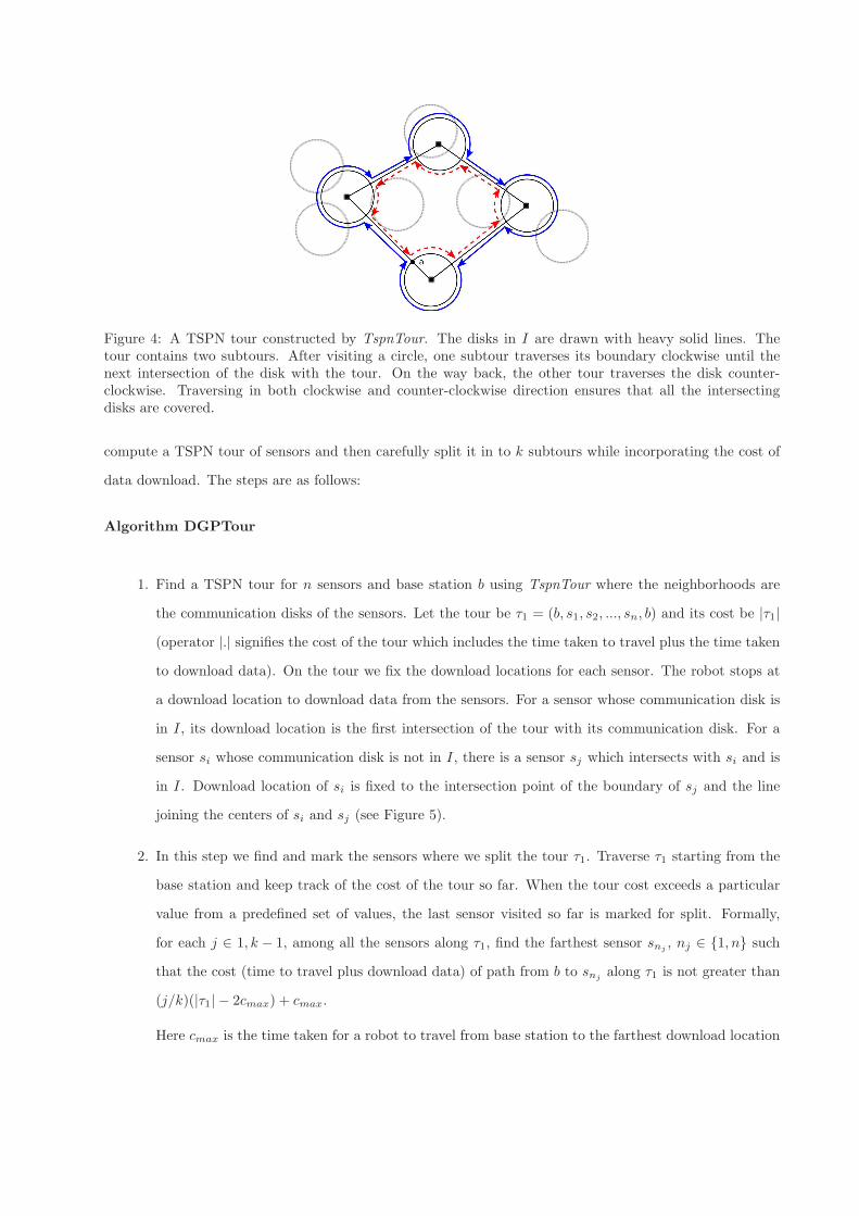
Figure 4: A TSPN tour constructed by TspnTour. The disks in I are drawn with heavy solid lines. Thetour contains two subtours. After visiting a circle, one subtour traverses its boundary clockwise until thenext intersection of the disk with the tour. On the way back, the other tour traverses the disk counter-clockwise. Traversing in both clockwise and counter-clockwise direction ensures that all the intersectingdisks are covered.
compute a TSPN tour of sensors and then carefully split it in to k subtours while incorporating the cost of
data download. The steps are as follows:
Algorithm DGPTour
1. Find a TSPN tour for n sensors and base station b using TspnTour where the neighborhoods are
the communication disks of the sensors. Let the tour be τ1 = (b, s1, s2, ..., sn, b) and its cost be |τ1|
(operator |.| signifies the cost of the tour which includes the time taken to travel plus the time taken
to download data). On the tour we fix the download locations for each sensor. The robot stops at
a download location to download data from the sensors. For a sensor whose communication disk is
in I, its download location is the first intersection of the tour with its communication disk. For a
sensor si whose communication disk is not in I, there is a sensor sj which intersects with si and is
in I. Download location of si is fixed to the intersection point of the boundary of sj and the line
joining the centers of si and sj (see Figure 5).
2. In this step we find and mark the sensors where we split the tour τ1. Traverse τ1 starting from the
base station and keep track of the cost of the tour so far. When the tour cost exceeds a particular
value from a predefined set of values, the last sensor visited so far is marked for split. Formally,
for each j ∈ 1, k − 1, among all the sensors along τ1, find the farthest sensor snj, nj ∈ {1, n} such
that the cost (time to travel plus download data) of path from b to snjalong τ1 is not greater than
(j/k)(|τ1| − 2cmax) + cmax.
Here cmax is the time taken for a robot to travel from base station to the farthest download location
from the base station.
3. After finding the sensors where the tour will split, we connect the base station to each of the marked
sensor and the sensor next to it on the tour τ1. Then we remove the edge on τ1 between the marked
sensor and the sensor next to it. This gives us k subtours. Or, let sji represents the ith sensor in jth
subtour. The jth subtour is represented by Rj = (b, sj1, sj
2, ..., sj
nj, b) for all j ∈ {1, k}, where sj
1is
the node next to sj−1
nj−1on the tour τ1.
In the following we show that the tour obtained by DGPTour is a constant factor away from the optimal
tour.
Theorem 2. If DGPTour returns τk as the maximum cost subtour among all k subtours, and τ∗k is the
maximum cost subtour in the optimal solution for the 2D Data Gathering Problem, then
|τk|/|τ∗k | ≤ e + 2− 1/k (2)
where e is the approximation ratio of the algorithm used to find TSPN tour at step 1 of our algorithm (in
our case approximation ratio of TspnTour).
Proof. The proof is similar to the proof of k − SplitTour algorithm for k-TSP presented in (Frederickson
et al., 1978). We show how the download times are incorporated.
First we claim that the cost of any subtour Ri produced by DGPTour is upper bounded by (1/k)(|τ1| −
2cmax) + 2cmax. The cost of the tour τ1 at sensor si1
is greater than ((i− 1)/k)(|τ1| − 2cmax) + cmax) (from
step 2) and the cost of the tour at sensor sini
is no more than ((i/k)(|τ1| − 2cmax) + cmax). Therefore, the
cost of the subtour Ri from sensor si1
to sini
is at most (1/k)(|τ1| − 2cmax). The cost of connecting the two
sensors si1
and sini
to the base station can be at most 2cmax. Hence,
|τk| = maxi∈{1,k}(|Ri|) ≤ (1/k)(|τ1| − 2cmax) + 2cmax (3)
Next, let τ∗1
be the optimal tour with 1 robot. We show that the cost of τ∗k is no less than 1
ktimes the cost
of τ∗1. Or, τ∗
k ≥1
kτ∗1. To prove this we create a new tour τ ′
1by merging all the k subtours of the optimal
solution. We order the subtours and connect the last sensor of each subtour to the first sensor of the next
subtour. We delete all but two of the edges joining the first and last sensor of these subtours to the base
station. We keep only two such edges, one from the base-station to the first sensor of the first subtour and
one from the base station to the last sensor of the last subtour. This gives us a tour τ ′1. For each edge added
we deleted two edges and all three of these edges form a triangle. Therefore by the triangle inequality, the
new edge will be no more than the sum of the edges deleted. This gives us |τ ′1| ≤ k|τ∗
k |. Also from optimality,
|τ ′1| ≥ |τ∗
1|, therefore,
τ∗k ≥
1
k|τ∗
1| (4)
Now we will find out the ratio |τ1||τ∗
1| . Let the cost of TSPN tour at step 1 of DGPTour with Td = 0 (only the
travel cost) be C and the cost of optimal TSPN tour with Td = 0 be C∗. We have |τ1| = C + nTd. Also
|τ∗1| ≥ max(C∗, nTd). Therefore,
|τ1|
|τ∗1|
=C + nTd
|τ∗1|
=C
|τ∗1|+
nTd
|τ∗1|
≤C
|C∗|+ 1 = e + 1 (5)
where e is the approximation ratio of the algorithm used to find the TSPN tour.
From Equation 3, Equation 4, Equation 5 and the fact that cmax ≤1
2|τ∗
k |, we get
|τk|/|τ∗k | ≤
(1/k)(|τ1| − 2cmax) + 2cmax
|τ∗k |
≤(1/k)|τ1| − (1/k)|τ∗
k |+ |τ∗k |
|τ∗k |
≤(1/k)|τ1|
|τ∗k |
− (1/k) + 1
≤|τ1|
|τ∗1|− (1/k) + 1 ≤ e + 2− 1/k. (6)
Figure 5 shows an instance where we use DGPTour to divide the tour into two subtours. By fixing the
download locations for each sensor, computing the cost of a part of the tour becomes straightforward. This
helps in splitting the tour in Step 2 of our algorithm.
4.3 Data Gathering Problem for Sparse Sensor Networks
In most data muling applications like environmental monitoring the sensors are deployed far apart. In such
scenarios TspnTour algorithm will have redundant parts because it traverses each edge joining the disks in

s1
s2
s3
s4
s5
s6
s7
s8
s9
R1
R2
b
Download LocationSensor
AB
Figure 5: Division of a TSPN tour into 2 subtours using DGPTour algorithm. Note that the second subtour(dashed lines) visits some sensors which were already visited by the first subtour (solid lines). This isbecause the original TSPN tour (computed by TSPNTour algorithm) visits the disks in both clockwise andanticlockwise directions to ensure that all the intersecting disks are visited. In this figure, the path from s8
to base station and back to s9 is not shown to increase clarity.
I (the maximal set of non-intersecting disks) twice. To deal with such scenarios we present an improvement
over TspnTour algorithm which saves travel cost by not visiting any edge more than once. We refer to the
improved algorithm by SparseTspnTour. We also formalize the notion of sparsity and provide the condition
when SparseTspnTour should be used instead of TspnTour.
b
a
Figure 6: This figure shows a TSPN tour computed by SparseTspnTour. It covers the boundary of each diskin I (the maximal set of non-intersecting disks) completely after visiting it once. This approach improvesthe coverage time when the communication disks are far apart.
Overview of the Algorithm SparseTspnTour: First, we compute a tour τI of disks in I similarly as in
TspnTour. We extend it to visit all the disks. To construct the tour start from the point of intersection
of the boundary of an arbitrary disk in I and τI . Traverse along τI until the point of intersection, a, of
the boundary of a disk belonging to I is encountered. Make a complete tour of the disk boundary until a
is encountered again. Now, from a traverse directly to the next point of intersection, b, of τI and this disk
(Figure 6). From b continue along τI in similar fashion until the point from where we started is reached.
Let the cost of τI in terms of distance be CI and the number of disks in I be m. Comparing with SparseT-
spnTour, TspnTour covers an extra distance of 1/2(CI − 2πmTr), since it traverses the tour twice. On the
other hand, SparseTspnTour covers an extra distance of up to 2mTr (along the diameter of the disk to get
back on the tour). Therefore, we can use SparseTspnTour whenever 2mTr ≤ 1/2(CI − 2πmTr). This gives
the condition
Tr ≤CI
2m(2 + π)(7)
When the condition in Equation 7 is satisfied SparseTspnTour performs better than TspnTour. The difference
in the cost is at least 1/2(CI − 2πmTr). This improvement can be significant in sparse sensor networks like
environmental monitoring networks where clusters of sensors are sparsely deployed over large areas. We
show in simulations that DGPTour based on SparseTspnTour performs better than the DGPTour based on
TspnTour. For the field experiments (Section 7) we use DGPTour algorithm based on SparseTspnTour.
5 Opportunistic DGP Algorithm
In this section, we present a modification of the DGP algorithm which alleviates some of the challenges faced
when executing it on a real system. In particular, there are two major challenges: First, the sensing and
actuation errors make it difficult to precisely follow the line segments output by the DGP algorithm. When
the robot steers off the computed path, it can be within the communication range of a sensor other than
the next sensor it is headed toward. Second, the disk model used for communication is not always accurate.
One can choose the disk radius conservatively so that the expected signal quality inside the disk is good.
However, occasionally it is possible to receive a good signal outside the disk. We now present a modification
of the DGP algorithm which opportunistically downloads from all sensors within the robots communication
range (Algorithm 1).
Let S = {s1, . . . sn} be the ordered list of sensors assigned to a robot u after the execution of the DGP
algorithm. We assume s1 be the base station so that robot starts its tour from the base in each tour. Let si
be the next sensor to visit in S. When running the opportunistic algorithm, the robot polls the sensors after
si and checks if they are within the communication range. Most WSN systems include low-level support for
scanning the communication channel. In our implementation, we utilize this capability of TelosB motes. If

the robot hears from any sensor sj such that j ≥ i, it stops and collects data from sj . The robot removes
sj from S, and continues toward si. After visiting the last node in S, the robot returns to s1 ignoring all
sensors heard in the mean time because their data has been downloaded recently.
Algorithm 1 OPPORTUNISTIC DGP ALGORITHM
1: Let S be the set of sensors assigned to robot u by DGP algorithm2: while S 6= ∅ do
3: Let si be the next sensor to visit4: if u hears a good signal from si or close enough to si then
5: Stop and collect data from si and set S ← S/si
6: else if u hears a good signal from a sensor sj such that j >= i then
7: Stop and collect data from sj .8: Set S ← S/sj and remove the visit of sj from the DGP tour9: else
10: Continue the tour returned by DGP algorithm11: Visit s1 for the next tour then Goto 1
6 Simulation Experiments
In this section, we further study DGP with simulations. We performed three simulation experiments. In the
first simulation, we investigated the utility of increasing the number of robots while keeping the number of
sensors fixed. In Figure 7, we plot the coverage time (travel time plus data download time) as a function
of k, the number of robots. For this experiment we placed 100 sensors uniformly at random in a 600× 600
environment. The communication radius Tr was chosen to be 30. As the figure shows, there is a steep decrease
in the cost as the number of robots increase initially. But when the number of robots start approaching the
number of independent disks (38 in this case), the decrement in the travel cost is not significant.
Figure 7: Coverage time as a function of robots for 100 sensors deployed uniformly at random in a 600×600area. Coverage time includes the time taken to visit all the disks and the time taken to download data fromthem.
In the second simulation, we compared the DGPTour based on TspnTour to DGPTour based on SparseT-
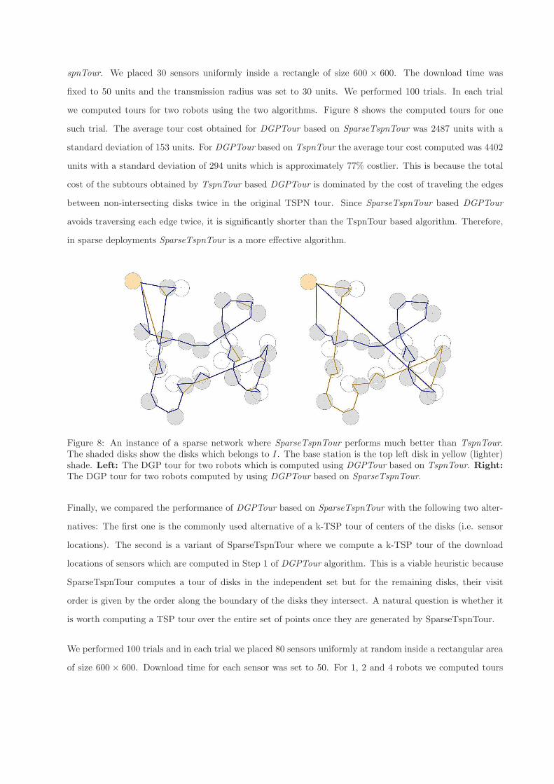
spnTour. We placed 30 sensors uniformly inside a rectangle of size 600 × 600. The download time was
fixed to 50 units and the transmission radius was set to 30 units. We performed 100 trials. In each trial
we computed tours for two robots using the two algorithms. Figure 8 shows the computed tours for one
such trial. The average tour cost obtained for DGPTour based on SparseTspnTour was 2487 units with a
standard deviation of 153 units. For DGPTour based on TspnTour the average tour cost computed was 4402
units with a standard deviation of 294 units which is approximately 77% costlier. This is because the total
cost of the subtours obtained by TspnTour based DGPTour is dominated by the cost of traveling the edges
between non-intersecting disks twice in the original TSPN tour. Since SparseTspnTour based DGPTour
avoids traversing each edge twice, it is significantly shorter than the TspnTour based algorithm. Therefore,
in sparse deployments SparseTspnTour is a more effective algorithm.
Figure 8: An instance of a sparse network where SparseTspnTour performs much better than TspnTour.The shaded disks show the disks which belongs to I. The base station is the top left disk in yellow (lighter)shade. Left: The DGP tour for two robots which is computed using DGPTour based on TspnTour. Right:
The DGP tour for two robots computed by using DGPTour based on SparseTspnTour.
Finally, we compared the performance of DGPTour based on SparseTspnTour with the following two alter-
natives: The first one is the commonly used alternative of a k-TSP tour of centers of the disks (i.e. sensor
locations). The second is a variant of SparseTspnTour where we compute a k-TSP tour of the download
locations of sensors which are computed in Step 1 of DGPTour algorithm. This is a viable heuristic because
SparseTspnTour computes a tour of disks in the independent set but for the remaining disks, their visit
order is given by the order along the boundary of the disks they intersect. A natural question is whether it
is worth computing a TSP tour over the entire set of points once they are generated by SparseTspnTour.
We performed 100 trials and in each trial we placed 80 sensors uniformly at random inside a rectangular area
of size 600 × 600. Download time for each sensor was set to 50. For 1, 2 and 4 robots we computed tours
Algorithms Number of
Robots
Cost difference with DGPTour as percentage
TransmissionRange: 40
TransmissionRange: 80
TransmissionRange: 120
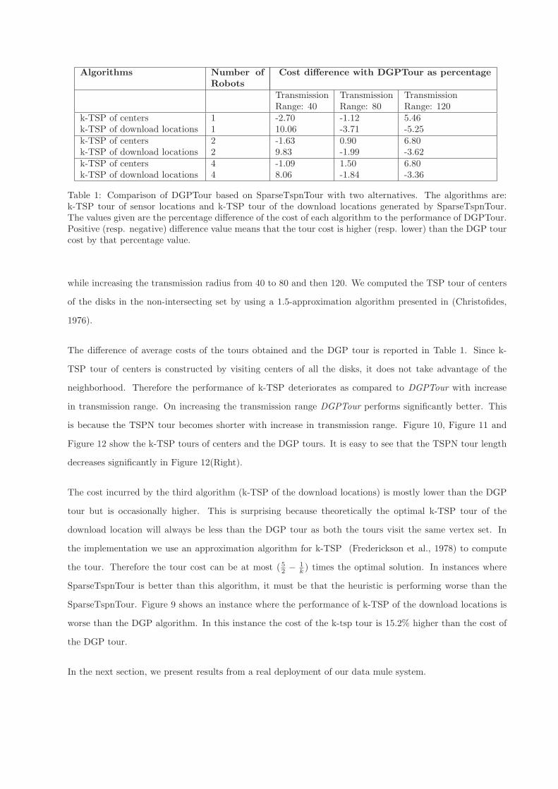
k-TSP of centers 1 -2.70 -1.12 5.46k-TSP of download locations 1 10.06 -3.71 -5.25k-TSP of centers 2 -1.63 0.90 6.80k-TSP of download locations 2 9.83 -1.99 -3.62k-TSP of centers 4 -1.09 1.50 6.80k-TSP of download locations 4 8.06 -1.84 -3.36
Table 1: Comparison of DGPTour based on SparseTspnTour with two alternatives. The algorithms are:k-TSP tour of sensor locations and k-TSP tour of the download locations generated by SparseTspnTour.The values given are the percentage difference of the cost of each algorithm to the performance of DGPTour.Positive (resp. negative) difference value means that the tour cost is higher (resp. lower) than the DGP tourcost by that percentage value.
while increasing the transmission radius from 40 to 80 and then 120. We computed the TSP tour of centers
of the disks in the non-intersecting set by using a 1.5-approximation algorithm presented in (Christofides,
1976).
The difference of average costs of the tours obtained and the DGP tour is reported in Table 1. Since k-
TSP tour of centers is constructed by visiting centers of all the disks, it does not take advantage of the
neighborhood. Therefore the performance of k-TSP deteriorates as compared to DGPTour with increase
in transmission range. On increasing the transmission range DGPTour performs significantly better. This
is because the TSPN tour becomes shorter with increase in transmission range. Figure 10, Figure 11 and
Figure 12 show the k-TSP tours of centers and the DGP tours. It is easy to see that the TSPN tour length
decreases significantly in Figure 12(Right).
The cost incurred by the third algorithm (k-TSP of the download locations) is mostly lower than the DGP
tour but is occasionally higher. This is surprising because theoretically the optimal k-TSP tour of the
download location will always be less than the DGP tour as both the tours visit the same vertex set. In
the implementation we use an approximation algorithm for k-TSP (Frederickson et al., 1978) to compute
the tour. Therefore the tour cost can be at most (5
2− 1
k) times the optimal solution. In instances where
SparseTspnTour is better than this algorithm, it must be that the heuristic is performing worse than the
SparseTspnTour. Figure 9 shows an instance where the performance of k-TSP of the download locations is
worse than the DGP algorithm. In this instance the cost of the k-tsp tour is 15.2% higher than the cost of
the DGP tour.
In the next section, we present results from a real deployment of our data mule system.
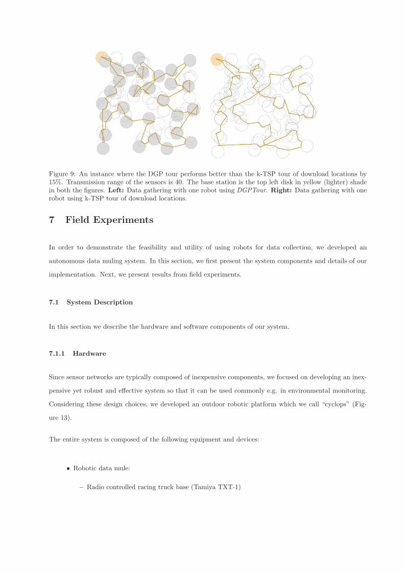
Figure 9: An instance where the DGP tour performs better than the k-TSP tour of download locations by15%. Transmission range of the sensors is 40. The base station is the top left disk in yellow (lighter) shadein both the figures. Left: Data gathering with one robot using DGPTour. Right: Data gathering with onerobot using k-TSP tour of download locations.
7 Field Experiments
In order to demonstrate the feasibility and utility of using robots for data collection, we developed an
autonomous data muling system. In this section, we first present the system components and details of our
implementation. Next, we present results from field experiments.
7.1 System Description
In this section we describe the hardware and software components of our system.
7.1.1 Hardware
Since sensor networks are typically composed of inexpensive components, we focused on developing an inex-
pensive yet robust and effective system so that it can be used commonly e.g. in environmental monitoring.
Considering these design choices, we developed an outdoor robotic platform which we call “cyclops” (Fig-
ure 13).
The entire system is composed of the following equipment and devices:
• Robotic data mule:
– Radio controlled racing truck base (Tamiya TXT-1)

Figure 10: Transmission range of the sensors is 40. The base station is the top left disk in yellow (lighter)shade in both the figures. Left: Data gathering with two robot using k-TSP. Right: Data gathering withtwo robots using DGPTour.
Figure 11: Transmission range of the sensors is 80. Left: The subtours computed by k-TSP does not changewith increase in transmission range. This is because k-TSP does not include the neighborhoods in computingthe tours. Right: On the other hand the subtours calculated by DGPTour shortens in length.
Figure 12: Transmission range of the sensors is 120. Left: Data gathering with two robot using k-TSP.Right: With higher transmission range, the subtours from DGPTour are significantly smaller than inFigure 10(Left)
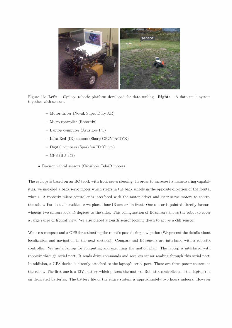
Figure 13: Left: Cyclops robotic platform developed for data muling. Right: A data mule systemtogether with sensors.
– Motor driver (Novak Super Duty XR)
– Micro controller (Robostix)
– Laptop computer (Asus Eee PC)
– Infra Red (IR) sensors (Sharp GP2Y0A02YK)
– Digital compass (Sparkfun HMC6352)
– GPS (BU-353)
• Environmental sensors (Crossbow TelosB motes)
The cyclops is based on an RC truck with front servo steering. In order to increase its maneuvering capabil-
ities, we installed a back servo motor which steers in the back wheels in the opposite direction of the frontal
wheels. A robostix micro controller is interfaced with the motor driver and steer servo motors to control
the robot. For obstacle avoidance we placed four IR sensors in front. One sensor is pointed directly forward
whereas two sensors look 45 degrees to the sides. This configuration of IR sensors allows the robot to cover
a large range of frontal view. We also placed a fourth sensor looking down to act as a cliff sensor.
We use a compass and a GPS for estimating the robot’s pose during navigation (We present the details about
localization and navigation in the next section.). Compass and IR sensors are interfaced with a robostix
controller. We use a laptop for computing and executing the motion plan. The laptop is interfaced with
robostix through serial port. It sends drive commands and receives sensor reading through this serial port.
In addition, a GPS device is directly attached to the laptop’s serial port. There are three power sources on
the robot. The first one is a 12V battery which powers the motors. Robostix controller and the laptop run
on dedicated batteries. The battery life of the entire system is approximately two hours indoors. However
IR
Compass
Robostix
Steer Servos GPS
Drive Motors
Eee PC
Base
Mote
Sensor
Mote
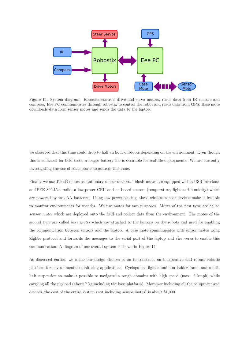
Figure 14: System diagram. Robostix controls drive and servo motors, reads data from IR sensors andcompass. Eee PC communicates through robostix to control the robot and reads data from GPS. Base motedownloads data from sensor motes and sends the data to the laptop.
we observed that this time could drop to half an hour outdoors depending on the environment. Even though
this is sufficient for field tests, a longer battery life is desirable for real-life deployments. We are currently
investigating the use of solar power to address this issue.
Finally we use TelosB motes as stationary sensor devices. TelosB motes are equipped with a USB interface,
an IEEE 802.15.4 radio, a low-power CPU and on-board sensors (temperature, light and humidity) which
are powered by two AA batteries. Using low-power sensing, these wireless sensor devices make it feasible
to monitor environments for months. We use motes for two purposes. Motes of the first type are called
sensor motes which are deployed onto the field and collect data from the environment. The motes of the
second type are called base motes which are attached to the laptops on the robots and used for enabling
the communication between sensors and the laptop. A base mote communicates with sensor motes using
ZigBee protocol and forwards the messages to the serial port of the laptop and vice versa to enable this
communication. A diagram of our overall system is shown in Figure 14.
As discussed earlier, we made our design choices so as to construct an inexpensive and robust robotic
platform for environmental monitoring applications. Cyclops has light aluminum ladder frame and multi-
link suspension to make it possible to navigate in rough domains with high speed (max. 6 kmph) while
carrying all the payload (about 7 kg including the base platform). Moreover including all the equipment and
devices, the cost of the entire system (not including sensor motes) is about $1,000.
7.1.2 Navigation Algorithms and Software
The software portion of our system consists of two components. The first component is an embedded program
developed for robostix. This component is implemented in C++ and provides an Application Programming
Interface (API) for controlling the robot and reading from compass and IR sensors. The second component
is developed for the laptop and used for high level control (navigation and sensory data download). Since we
have various sensors which have to be read in parallel, we implemented a multi-threaded system. A separate
thread reads and writes from/to each device (compass, GPS, robostix and base mote) and updates its state
in the main thread. Since Java provides an advanced threading scheme, we used Java to implement the high
level application. We also implemented a server/client application and a GUI to visualize the robot’s state
from a remote computer.
Motes are programmed in nesC. Sensing motes send simple beacon messages, while the base mote receives
these messages and filters them according to their mote ids. Messages coming from the target mote are
processed in the base mote. The base computes the link quality indicator (LQI) values of the packets
received and sends them as serial packets to the Java program running on the laptop. The java program
saves the timestamps (start and end time of the download) and packets received.
The DGP algorithm in Section 4.3 yields way-points to be visited along with the ids of sensors whose
data must be downloaded at each way-point. We now describe the algorithm for navigating between these
way-points.
The robot uses only compass and GPS for pose estimation. Since neither sensor provides accurate informa-
tion, the robot has to deal with large uncertainties during navigation. At the beginning of its tour, the robot
executes an initialization routine to ensure that it receives the most accurate readings from these devices.
The compass requires an initial calibration step to adjust its values according to the earth’s magnetic field
and external electro-magnetic fields. For that purpose, robot loops around a circle twice at the beginning
and calibrates its compass. Afterward the robot uses only compass measurements to determine its heading.
It is well-known that GPS performance changes according to external factors (e.g. environmental effects, and
the number and configuration of satellites). To improve its accuracy, we enabled Wide Area Augmentation
System (WAAS) feature of our GPS device which corrects for GPS signal errors caused by ionospheric
disturbances, timing, and satellite orbit errors. Moreover, we determined that GPS accuracy is higher when
robot is moving compared to when it is stationary. Hence, initially to get a better estimate, the robot moves
on a straight line until the variance of the heading measurements drops below a threshold. After good GPS
measurements are obtained, the robot computes its desired heading by using its current location and the
target location (next way-point). The robot uses its compass to move in the desired direction. However,
due to errors, sometimes it goes off of the desired trajectory. The opportunistic algorithm presented in
Section 5 overcomes some of the inefficiencies associated with this type of error. When the error goes beyond
a threshold, the robot re-computes its trajectory to the next node. In experiments described next, the
uncertainty of GPS measurements was about 3 meters.
7.2 Experiments
In this section we present field experiments conducted by the system discussed above. These experiments
are designed for two reasons. First we aim to show the practical feasibility of using an inexpensive robot as
a data mule for collecting data from sensors. Second we aim to show how our algorithm can be improved
in practice under navigation and communication uncertainties. For this purpose we conducted two sets of
experiments. In the first experiment we showed the feasibility of our system using DGP algorithm presented
in Section 4.3. Using observations from the first experiment, we extended our algorithm by using the
opportunistic approach presented in Section 5. Since we have only one robot, our experiments do not involve
multiple robots. However, since the DGP algorithm partitions the sensors among the robots and robots do
not communicate during the data collection, in a single robot is sufficient to accomplish our goals.
All experiments were conducted in East River Flats near the Mississippi River/Minnesota. The ground
surface of this field is mainly covered with long grass which makes it a challenging environment for navigation.
See Figure 15. We placed seven sensors (S = {S0, . . . , S6}) in a rectangular area of approximate size of
170m×70m. Since a base and a sensor are treated as identical disks, we did not deploy a specific base.
Instead, we treat the last sensor as the base station. Sensors’ communication range was set to 6m. In our
deployment, the communication disks of sensors S0, S1 and S2 overlap as well as the communication disks
of sensors S4 and S5 which were placed at the top of a hill.
We computed a tour for this deployment using the SparseTspnTour algorithm presented in Section 4.3.
SparseTspnTour chose S0, S3, S4 and S6 as sensors with non-overlapping communication disks in I.
For each overlapping sensor we compute a download location. The ordered tour is given by: τ =
{D0,D1,D2,D3,D4,D5,D6}. The robot was programmed to download twenty packets of size 32 bytes
from each sensor where each sensor was programmed to send packets as beacons with time interval 250
milliseconds.

Tour-1 Tour-2Download time Travel Time Download Time TravelTime
S0 4.9 5.3 151.1S1 5.1 12.2 5.9 26.0S2 5.1 1.2 4.8 0.9S3 5.0 100.0 5.1 113.7S4 4.9 26.7 4.9 33.9S5 4.8 64.5 4.8 57.3S6 5.0 41.7 30.0 100.5Total 34.84 246.2 60.93 483.33Tour Total 825.3
Table 2: Download and travel times in seconds from the DGP experiment. The first row of Tour-2 includesthe time to travel from S6 to S0.
In the first experiment we made the robot execute the tour τ . Due to GPS uncertainties we programmed
the robot to stop if its distance to destination point Di is closer than some threshold. Moreover during
our initial experiments we realized that the robot occasionally hears good signal from long distances while
moving towards the target sensor due the environmental effects. For example robot was able hear the sensor
at the top of the hill (S4) from approximately 25m distance. In these cases robot does not have to navigate
all the way to the desired download location. Hence we modified our algorithm by adding the following
condition: robot collects data from sensor Si if it is close enough to Di or it hears a good signal from Si.
Note that this modification does not allow downloading from nodes out of order. It simply changes the
download location if a better signal becomes available early on.
Left and right images in Figure 16 show the GPS trace of the robot during the first and the second tours
respectively. The actual download locations were marked with the different placemarks and labeled as
{F0, . . . , F6}. The actual and intended download locations were different due to the uncertainty in GPS
readings and the modification regarding the download location. The download, travel and total times are
reported in Table 2. We also include the total tour time as the sum of download and travel times.
Since the actual starting positions in this experiment and the next one were different, we started the first
tour from S0. Hence the travel time to reach S0 was not counted in the first tour. However in the second
tour the travel time from S6 to S0 was counted as the travel time to reach this sensor. Observe that the
download times are consistent with each other except the last sensor in the second tour. This is because,
while moving towards S6 robot heard a temporary good signal from S6 and stopped. However the signal
strength dropped during the download which extended the download time.
In the first experiment, we realized that the robot hears from other sensors while moving towards target

Tour-1 Tour-2Download time Travel Time Download Time TravelTime
S0 4.8 5.0 97.5S1 4.8 46.6 4.7 8.1S2 5.0 0 5.3 13.4S3 4.8 113.3 6.3 111.4S4 5.8 28.5 5.7 35.0S5 4.9 47.6 8.2 72.5S6 5.9 42.8 5.6 91.2Total 36.08 278.75 40.93 429.07Tour Total 784.82
Table 3: Download and travel times in seconds from the opportunistic DGP experiment. The first row ofTour-2 includes the time to travel from S6 to S0.
location. This specially happens when robot is collecting data from overlapping sensors. For example,
when robot is moving towards S1, sometimes it hears a good signal from S2 before S1. In this case robot
can download data from S2 and therefore can eliminate the traveling cost to S2. Hence we proposed an
opportunistic version of the DGP algorithm which is presented in detail in Section 5. In contrast to download
location modification, this modification allows robot to download from any node that the robot can hear
which consequently changes the order of the tour.
Left and Right of Figure 17 show the GPS trace from the opportunistic DGP experiment. The download
and travel times during this experiment are reported in Table 3. In this experiment robot leverages the
opportunistic approach to reduce its tour time. The total travel time in the first experiment was 730 seconds
whereas in the opportunistic DGP experiment the total travel time was 708 seconds. However it is hard make
a reliable comparison between the two strategies since the actual paths and the actual download locations
were different. On the other hand we can see the advantage of the opportunistic approach when robot
downloads data from S2 in the first tour. Since S0, S1 and S2 were close robot heard a good signal from S2
when moving from S0 to S1 and download the data on the way. Hence it did not spend extra time to visit
S2 which otherwise it would have spent about 13 seconds to navigate to D2 as in the second tour.
Next we compute how much the robot deviates from the ideal solution shown in Figure 15. The length of
the ideal tour is 550m. The length of the robot’s path in the first experiment was 625m. In the second
experiment (opportunistic) this length was 629m. Therefore the uncertainties increase the tour length by
13.6% and 14.3% respectively. In terms of download times ideal solution would have spent at least 65.8
seconds to download data from all the sensors (assuming 4.7 seconds download time from each sensor). On
the other hand in the first and the second experiments the total download times were 95.8 and 77 seconds,
respectively. These yield to 45.6% and 17% increase in the download times. In terms of total tour times
ideal solution would spend 615.8 seconds to finish two tours assuming a 1 m/sec average speed. The total
tour times in the first and the second experiments were 825.3 and 784.8 seconds respectively. Hence the
overall deviations from the ideal solution were 34% and 27.4%.
Although the number of experiments conducted were limited, the results show that despite the navigation and
communication uncertainties, the performance of the system was not too far from the ideal solution. More
importantly, they demonstrate that a data muling system built from inexpensive off-the-shelf components is
feasible. In the future we aim to reduce navigational uncertainties by improving our algorithms and hardware
capabilities.
8 Conclusion
In this paper, we studied a path planning problem, the Data Gathering Problem (DGP), which arises in
scenarios where robots act as data mules to download data from stationary wireless devices. The problem
differs from the well-known TSP problem due to the fact that downloading data takes time. Therefore, the
cost of a tour is effected by not only the travel time but also the download time as well as the number of
downloads.
We presented an optimal, polynomial-time algorithm for a special case where the robots are restricted to
move along a curve which contains the base station at one end. This case is applicable in scenarios where
the robots are restricted to move along a predetermined path such as a railroad track. For the 2D version,
we showed that two algorithms developed for variants of the TSP problem can be combined and adapted
to obtain a constant factor approximation algorithm for DGP in 2D. We also presented an improvement for
sparse networks where robots spend significant time to travel between clusters that are far away.
We implemented the algorithm on a data muling system. Results from a field experiment demonstrated the
effectiveness and utility of the system. We are currently working on improving the lifetime of our system
using renewable energy sources such as solar. Our current design assigns each sensor to a single robot. It
may be beneficial to allow the robots to communicate with each other. Our future work includes further
exploring this multi-robot communication/cooperation aspect of data muling.

9 Acknowledgment
This work is supported in part by NSF grants 0916209, 0917676 and 0936710. The authors thank Pratap
Tokekar for his help in developing the cyclops robot platform.
10 Appendix A: Index to Multimedia Extensions
Extension Media Type Description
1 Video Video record of our proof of concept experiment
References
Anastasi, G., Conti, M., and Di Francesco, M. (2008). Data collection in sensor networks with data mules:
An integrated simulation analysis. pages 1096 –1102, Marrakech,Morocco.
Anastasi, G., Conti, M., Monaldi, E., and Passarella, A. (2007). An adaptive data-transfer protocol for
sensor networks with Data Mules. In IEEE International Symposium on a World of Wireless, Mobile
and Multimedia Networks, pages 1–8, Helsinki, Finland.
Applegate, D. L., Bixby, R. E., Chvatal, V., and Cook, W. J. (2006). The Traveling Salesman Problem: A
Computational Study. Princeton University Press.
Beaufour, A., Leopold, M., and Bonnet, P. (2002). Smart-tag based data dissemination. In Proceedings
of the 1st ACM International Workshop on Wireless Sensor Networks and Applications, pages 68–77,
Atlanta, GA, USA. ACM.
Bhadauria, D. and Isler, V. (2009). Data gathering tours for mobile robots. In IEEE International Conference
on Intelligent Robots and Systems, pages 3868–3873, St. Louis, MO, USA. IEEE Press.
Boloni, L. and Turgut, D. (2008). Should I send now or send later? A decision-theoretic approach to
transmission scheduling in sensor networks with mobile sinks. Wireless Communications and Mobile
Computing, 8(3):385–403.
Chakrabarti, A., Sabharwal, A., and Aazhang, B. (2003). Using predictable observer mobility for power
efficient design of sensor networks. In Proceedings of the 2nd International Conference on Information
Processing in Sensor Networks, pages 129–145, Palo Alto, CA, USA. Springer-Verlag.
Christofides, N. (1976). Worst case analysis of a new heuristic for the traveling salesman problem. Technical
report, Graduate School of Industrial Administration.
Dumitrescu, A. and Mitchell, J. S. B. (2003). Approximation algorithms for tsp with neighborhoods in the
plane. J. Algorithms, 48(1):135–159.
Dunbabin, M., Corke, P., Vasilescu, I., and Rus, D. (2006). Data muling over underwater wireless sensor
networks using an autonomous underwater vehicle. pages 2091–2098, Orlando, FL, USA.
Ekici, E., Gu, Y., and Bozdag, D. (2006). Mobility-based communication in wireless sensor networks. IEEE
Communications Magazine, 44(7):56.
Frederickson, G. N., Hecht, M. S., and Kim, C. E. (1978). Approximation algorithms for some routing
problems. SIAM Journal on Computing, 7(2):178–193.
Gasparri, A., Krishnamachari, B., and Sukhatme, G. (2008). A framework for multi-robot node coverage in
sensor networks. Annals of Mathematics and Artificial Intelligence, 52(2):281–305.
Gu, Y., Bozdag, D., Ekici, E., Ozguner, F., and Lee, C. (2005). Partitioning based mobile element scheduling
in wireless sensor networks. In Second Annual IEEE Communications Society Conference on Sensor
and Ad Hoc Communications and Networks, pages 386–395, Santa Clara, CA, USA.
Jea, D., Somasundara, A., and Srivastava, M. (2005). Multiple controlled mobile elements (data mules) for
data collection in sensor networks. pages 244–257, Marina del Rey, CA, USA. Springer.
Juang, P., Oki, H., Wang, Y., Martonosi, M., Peh, L., and Rubenstein, D. (2002). Energy-efficient computing
for wildlife tracking: Design tradeoffs and early experiences with zebranet. ACM SIGOPS operating
systems review, 36(5):96–107.
Kansal, A., Somasundara, A. A., Jea, D. D., Srivastava, M. B., and Estrin, D. (2004). Intelligent fluid
infrastructure for embedded networks. In International Conference on Mobile Systems, Applications,
and Services, pages 111–124, Boston, MA, USA.
Ma, J., Chen, C., and Salomaa, J. P. (2008). mWSN for large scale mobile sensing. J. Signal Processing
Systems, 51(2):195–206.
Mitchell, J. S. B. (2007). A ptas for tsp with neighborhoods among fat regions in the plane. In Proceedings
of the Eighteenth Annual ACM-SIAM Symposium on Discrete Algorithms, pages 11–18, Philadelphia,
PA, USA. Society for Industrial and Applied Mathematics.

Shah, R. C., Roy, S., Jain, S., and Brunette, W. (2003). Data mules: Modeling and analysis of a three-tier
architecture for sparse sensor networks. Ad Hoc Networks, 1(2–3):215–233.
Sugihara, R. and Gupta, R. (2010). Optimal speed control of mobile node for data collection in sensor
networks. Mobile Computing, IEEE Transactions on, 9(1):127 –139.
Tekdas, O., Lim, J., Terzis, A., and Isler, V. (2009). Using mobile robots to harvest data from sensor fields.
IEEE Wireless Communications, 16(1):22–28.
Tirta, Y., Li, Z., Lu, Y.-H., and Bagchi, S. (2004). Efficient collection of sensor data in remote fields using
mobile collectors. pages 515–519, Chicago, IL, USA.
Williams, K. and Burdick, J. (2006). Multi-robot boundary coverage with plan revision. In IEEE Interna-
tional Conference on Robotics and Automation, pages 1716–1723.
Wu, F., Huang, C., and Tseng, Y. (2009). Data gathering by mobile mules in a spatially separated wireless
sensor network. In International Conference on Mobile Data Management: Systems, Services and
Middleware, pages 293–298, Taipei,Taiwan. IEEE Computer Society.
Xing, J., Wang, H., Han, K., Ray, D., Huang, C., Chemnick, L., Stewart, C., Disotell, T., Ryder, O., and
Batzer, M. (2005). A mobile element based phylogeny of Old World monkeys. Molecular Phylogenetics
and Rvolution, 37(3):872–880.
Yuan, B., Orlowska, M., and Sadiq, S. (2007). On the optimal robot routing problem in wireless sensor
networks. IEEE Trans. on Knowl. and Data Eng., 19(9):1252–1261.
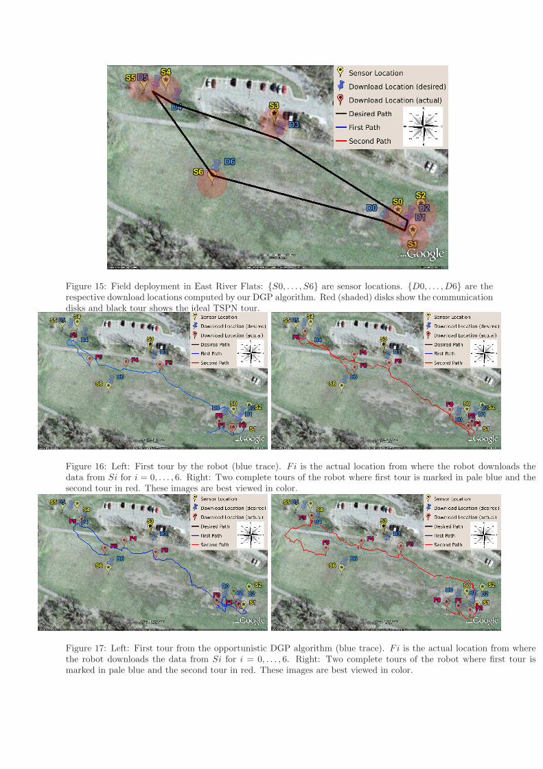
Figure 15: Field deployment in East River Flats: {S0, . . . , S6} are sensor locations. {D0, . . . ,D6} are therespective download locations computed by our DGP algorithm. Red (shaded) disks show the communicationdisks and black tour shows the ideal TSPN tour.
Figure 16: Left: First tour by the robot (blue trace). Fi is the actual location from where the robot downloads thedata from Si for i = 0, . . . , 6. Right: Two complete tours of the robot where first tour is marked in pale blue and thesecond tour in red. These images are best viewed in color.
Figure 17: Left: First tour from the opportunistic DGP algorithm (blue trace). Fi is the actual location from wherethe robot downloads the data from Si for i = 0, . . . , 6. Right: Two complete tours of the robot where first tour ismarked in pale blue and the second tour in red. These images are best viewed in color.