ROBOTIC ARM USING STEP MOTORS: STUDIES FOR OPTIMAL

DANILO HENRIQUE COSTA SOUZA

ROBOTIC ARM USING STEP MOTORS:STUDIES FOR OPTIMAL OPERATION AND

LOAD MASS ESTIMATION

Sao Paulo2021




Dissertation submitted to Escola

Politecnica of the Universidade de Sao

Paulo for degree of Master in Science.

Sao Paulo2021




Revised Version

Dissertation submitted to Escola

Politecnica of the Universidade de Sao

Paulo for degree of Master in Science.

Concentration area:

Systems engineering

Advisor:

Prof. Dr. Diego Colon

Sao Paulo2021

ACKNOWLEDGMENTS

To my wife for the support during the study times and the understanding during theabsence times.

To my teacher and advisor Diego Colon for the countless hours of guidance throughthis work and for embracing the idea.

“Love is the one thing that transcendstime and space.“

-Interstellar, 2014.-

RESUMO

Motores de passo podem ser descritos como motores DC digitais onde e possıvel obterum movimento preciso e bem definido. Entretanto, sao sistemas nao-lineares bastantecomplexos os quais precisam de um driver especıfico para realizar a interface entre omotor e o controlador digital a fim de obter o desempenho desejado. Os componentessupracitados formam um Step System e sao a forma mais comum de utilizacao de motoresde passo. O driver, incluıdo nas analises e simulacoes realizadas, proporciona um cenariomais proximo de uma sistema pratico. Este trabalho combina as equacoes eletricas emecanicas do modelo do motor de passo com as equacoes dinamicas de um braco roboticode um grau de liberdade, com o intuito analisar o desempenho do sistema por meiode um framework, a analise proposta e realizada via Simulink c© e inclui a modelagemcompleta do driver, consistindo em analisar o tempo, o passo medio do motor e a eficienciaenergetica do sistema completo. O Objetivo final e propor um metodo para estimacao damassa da carga quando o motor esta parado com corrente fluindo nas bobinas.

Palavras-Chave: Motor de passo, micro passo, carga dinamica, analise de desempenho,chopper driver.

ABSTRACT

Step motors can be described as digital DC motors where it is possible to obtain avery precise and fixed motion. They are, however, a rather complex non linear systemsthat need a specific driver for interfacing with a digital controller in order to achieve thedesired performance. The aforementioned components compose a so called Step Systemand are the most common way of operating a step motor. The step driver, included inthe simulations and analysis here performed, makes the scenario more close to a practicalone. This work combines the step motor electrical and mechanical equations, with thedynamics of a 1 DOF robotic arm to analyse the performance of the system through aperformance analysis framework, performed via Simulink c© including the model of thedriver, which consists of analysing the time, the mean of the actual stepped angle of themotor and energy efficiency and consumption of the whole system. The final goal is topropose a method to estimate the mass of the load when the motor is stopped with currentflowing through its windings.

Keywords: Step motor, micro stepping, step driver, dynamic load, performance analysis,chopper driver.

LIST OF FIGURES

1 Layers of a coconut. . . . . . . . . . . . . . . . . . . . . . . . . . . . . . . . 21

2 Work positions of the arm. . . . . . . . . . . . . . . . . . . . . . . . . . . . 23

3 Cross section of a step motor. . . . . . . . . . . . . . . . . . . . . . . . . . 24

4 Representative drawing of a step system. . . . . . . . . . . . . . . . . . . . 25

5 Block diagram of a closed-loop step system. . . . . . . . . . . . . . . . . . 26

6 Permanent magnet step motor excitation sequence. . . . . . . . . . . . . . 32

7 Variable reluctance motor axis section. . . . . . . . . . . . . . . . . . . . . 33

8 Hybrid step motor side and top views . . . . . . . . . . . . . . . . . . . . . 33

9 Bipolar and unipolar driver circuits. . . . . . . . . . . . . . . . . . . . . . . 36

10 Step motor different excitation modes. . . . . . . . . . . . . . . . . . . . . 37

11 Constant voltage driver circuit example. . . . . . . . . . . . . . . . . . . . 38

12 Constant voltage waveform example. . . . . . . . . . . . . . . . . . . . . . 39

13 Current-forced driver circuit example. . . . . . . . . . . . . . . . . . . . . . 39

14 Current-forced wave form example. . . . . . . . . . . . . . . . . . . . . . . 40

15 Chopper driver circuit example. . . . . . . . . . . . . . . . . . . . . . . . . 40

16 Chopper driver wave form example. . . . . . . . . . . . . . . . . . . . . . . 41

17 TorqueXSpeed curve for the motor KTC-HT34-487. . . . . . . . . . . . . 41

18 TorqueXSpeed curve for the motor KTC-110HS165. . . . . . . . . . . . . 42

19 Worm gearbox detail. . . . . . . . . . . . . . . . . . . . . . . . . . . . . . . 44

20 TorqueXSpeed graph of the step motor 86HS82-4504A14-B35-02 . . . . . 45

21 Robotic arm. . . . . . . . . . . . . . . . . . . . . . . . . . . . . . . . . . . 47

22 Default power stepper motor module diagram. . . . . . . . . . . . . . . . . 54

23 Default driver module diagram. . . . . . . . . . . . . . . . . . . . . . . . . 55

24 Modified driver module diagram. . . . . . . . . . . . . . . . . . . . . . . . 55

25 Diagram of the motor’s module. . . . . . . . . . . . . . . . . . . . . . . . . 56

26 Details of the motor’s module. . . . . . . . . . . . . . . . . . . . . . . . . . 57

27 Angle output of one simulation from the power stepper motor module. . . . 58

28 Step angle δθ output of one simulation from the power stepper motor module. 59

29 Average step angle µδθ for several simulations at different speeds and the

same reference angle θref . . . . . . . . . . . . . . . . . . . . . . . . . . . . 60

30 Surfaces plot for three different initial angles. . . . . . . . . . . . . . . . . . 62

31 Block diagram of the closed loop system. . . . . . . . . . . . . . . . . . . . 63

32 Modified Simulink c© model. . . . . . . . . . . . . . . . . . . . . . . . . . . 64

33 Simulation results for ωmax = 0.9817 rad/s . . . . . . . . . . . . . . . . . . 66



36 Simulation results when ωmax is not defined (the controller has no upper

saturation) . . . . . . . . . . . . . . . . . . . . . . . . . . . . . . . . . . . . 67

37 Efficiency analysis by time. . . . . . . . . . . . . . . . . . . . . . . . . . . . 70

38 Efficiency analysis by mean stepped. . . . . . . . . . . . . . . . . . . . . . 71

39 Energy analysis. . . . . . . . . . . . . . . . . . . . . . . . . . . . . . . . . . 72

40 Energy flow diagram for an operation of the arm. . . . . . . . . . . . . . . 73

41 Mass signal m∗gavg(kN) sampled at 10µs. . . . . . . . . . . . . . . . . . . . 78

42 Mass signal m∗gavg(kN) sampled at 10ms. . . . . . . . . . . . . . . . . . . . 79

43 Mass signal m∗gavg(kN) sampled at 10µs for 3 different values of mg. . . . . 79

44 Mass signal m∗gavg(kN) sampled at 10ms for 3 different values of mg. . . . . 80

LIST OF TABLES

1 Mass estimation results. . . . . . . . . . . . . . . . . . . . . . . . . . . . . 80

LIST OF SYMBOLS

θ1 Angle of the arm with respect to the horizontal axis

θm Angle of the motor’s axis with respect to the horizontal axis

θ1 Arm’s speed

θ1(t) Acceleration of the arm

τl Load torque

ij(t) Current on the j-th phase of the step motor

mg Mass of the grip

τL Load torque

v Velocity vector of the load

δθ Step angle of the step motor

τf Torque needed to move the load

τm Torque of the motor

Np Total number of pulses to move the motor through a given distance

tsim Power step motor module simulation time in Simulink c©

PPSref Driver reference frequency given in pulses per second

LIST OF ACRONYMS

c.g Center of Gravity

D.O.F. Degree of Freedom

RMS Root Mean Square

IC Integrated Circuit

CNC Computer Numeric Control

PWM Pulse Width Modulation

RPM Rotations Per Minute

PM Permanent Magnet

MOSFET Metal-Oxide-Semiconductor Field Effect Transistor

PCB Printed Circuit Board

VDC Voltage DC

PLC Programmable Logic Controller

EMF Electromotive force

PPR Pulses Per Revolution

PPS Pulses Per Second

AI Artificial Intelligence

CONTENTS

1 Introduction 21

1.1 The motivating problem . . . . . . . . . . . . . . . . . . . . . . . . . . . . 21

1.2 Step motors . . . . . . . . . . . . . . . . . . . . . . . . . . . . . . . . . . . 24

1.2.1 Open loop x closed loop . . . . . . . . . . . . . . . . . . . . . . . . 25

1.3 Related works . . . . . . . . . . . . . . . . . . . . . . . . . . . . . . . . . . 26

1.4 Objectives . . . . . . . . . . . . . . . . . . . . . . . . . . . . . . . . . . . . 28

1.5 Structure of the thesis . . . . . . . . . . . . . . . . . . . . . . . . . . . . . 29

1.6 Publications . . . . . . . . . . . . . . . . . . . . . . . . . . . . . . . . . . . 29

2 Step Motor Fundamentals and Criteria for Selection 31

2.1 Types of step motors . . . . . . . . . . . . . . . . . . . . . . . . . . . . . . 32

2.1.1 Permanent magnet . . . . . . . . . . . . . . . . . . . . . . . . . . . 32

2.1.2 Variable reluctance . . . . . . . . . . . . . . . . . . . . . . . . . . . 32

2.1.3 Hybrid step motor . . . . . . . . . . . . . . . . . . . . . . . . . . . 33

2.2 Step motor model . . . . . . . . . . . . . . . . . . . . . . . . . . . . . . . . 33

2.3 Step motor driving . . . . . . . . . . . . . . . . . . . . . . . . . . . . . . . 35

2.3.1 Driver operation types . . . . . . . . . . . . . . . . . . . . . . . . . 38

2.3.1.1 Constant-voltage driver . . . . . . . . . . . . . . . . . . . 38

2.3.1.2 Current-forced driver . . . . . . . . . . . . . . . . . . . . . 39

2.3.1.3 Constant current (chopper driver) . . . . . . . . . . . . . . 40

2.4 The γ factor . . . . . . . . . . . . . . . . . . . . . . . . . . . . . . . . . . . 42

2.5 Step motor selection . . . . . . . . . . . . . . . . . . . . . . . . . . . . . . 43

2.5.1 Driver selection . . . . . . . . . . . . . . . . . . . . . . . . . . . . . 43

2.5.2 Gearbox selection . . . . . . . . . . . . . . . . . . . . . . . . . . . . 43

2.5.3 Step-by-step guide of step motor selection . . . . . . . . . . . . . . 44

3 The Robotic Arm 47

3.1 Equations of the arm . . . . . . . . . . . . . . . . . . . . . . . . . . . . . . 47

3.2 Mathematical model for the complete mechanical system . . . . . . . . . . 49

3.2.1 Equilibrium analysis . . . . . . . . . . . . . . . . . . . . . . . . . . 51

4 Step System Optimal Operation: Simulation Results 53

4.1 Driver and hybrid step motor Simulink c© model . . . . . . . . . . . . . . 53

4.1.1 The driver module . . . . . . . . . . . . . . . . . . . . . . . . . . . 54

4.1.2 The motor module . . . . . . . . . . . . . . . . . . . . . . . . . . . 56

4.2 Open loop scenario . . . . . . . . . . . . . . . . . . . . . . . . . . . . . . . 57

4.3 Closed loop scenario . . . . . . . . . . . . . . . . . . . . . . . . . . . . . . 63

4.3.1 Description . . . . . . . . . . . . . . . . . . . . . . . . . . . . . . . 63

4.3.2 Examples . . . . . . . . . . . . . . . . . . . . . . . . . . . . . . . . 65

4.3.3 Objective of the present application . . . . . . . . . . . . . . . . . . 68

4.3.4 Performance analysis framework . . . . . . . . . . . . . . . . . . . . 68

4.3.4.1 Parameters definition . . . . . . . . . . . . . . . . . . . . . 68

4.3.4.2 Parameters analysis . . . . . . . . . . . . . . . . . . . . . 69

5 Load Mass Estimation 75

5.1 Mass estimation importance . . . . . . . . . . . . . . . . . . . . . . . . . . 75

5.2 The proposed approach . . . . . . . . . . . . . . . . . . . . . . . . . . . . . 76

6 Conclusions and Future Work 81

References 83

21

1 INTRODUCTION

This chapter presents an introduction of the problem to be analysed

as well as a literature review on the matter and the structure of this

work.

1.1 The motivating problem

The problem behind this work comes from a machine developed for paring the co-

conut’s skin, as one of the last steps in coconut processing. The machine must process a

half of a coconut at a time. The coconut half is placed on a table and transported by a

one degree of freedom robotic arm, known as the feeder arm, to the next step, which is

the paring table, that will do the actual work of removing the coconut’s skin. Figure 1

shows a coconut and it’s layers.

Figure 1: Layers of a coconut.Source: The author

The feeder arm is driven by a NEMA 34 step motor powered by an external 6A step

driver. This driver was built specifically for this application using an external MOSFET’s

driver and a microcontroller for interfacing. The need to built a specially designed driver

comes from the fact that the arm is heavy and even though a gear-box is used to counter-

balance the hight torque needed, this leads to the most common problem when it comes

to step motors: the Speed X Torque curve, that is, using high torque in a high speed

application implies step loss, hence the need to perform a careful selection.

22

Most of step motor papers do not clearly indicate, or do not use, a model for the load

torque and usually simulates the equations of the motor using a step input voltage. This

work intends to combine both step motor’s electrical and mechanical models with the

dynamic model of a 1 D.O.F robotic arm to study its behaviour when transporting a non

static load through long distances, usually higher than 10 times the base step δθ = 1.8o.

Energizing a step motor is a far complex task and it is usually done by an external driver.

This work analyses the behaviour of a step motor when energized by a step driver. The

driver controls the current on the motor’s windings via PWM voltage (detailed in Section

2.3).

Also, it is desired to control the arm’s displacement from one given position to another

in minimum time. The arm is not supposed to move at a target speed, but it is required

to move a fixed distance in minimum time. The frequency in which the chosen step

motor will begin to not respond to command pulses gives the upper boundary speed for

the system and, therefore, is the time limiting factor of the problem. Before presenting

the operation of the arm, it is important to properly reference the reader for the angles

variables used in this work. In the reference chosen, the load angle θL is equal to the

motor’s angle θm (detailed in section 3.1), which may also be referred to as θ1.

The total displacement required for the arm to move varies and there are four states

(positions) that the arm can be stationary while waiting to move again. They are:

1. Wait Load: Position where the arm waits the command to pick up the coconut

(θL = 135o);

2. Load: Position where the arm picks up the coconut (θL = 180o);

3. Wait Unload: Position where the arm waits the command to place the coconut at

the paring table (θL = 45o);

4. Unload: Position where the arm releases the coconut at the paring table (θL = 0o).

Figure 2 shows a full cycle, from picking up the coconut to place it at the paring table

of the feeder arm operation.

This arrangement with the feeder arm to place the coconuts into the machine gives

the possibility of adding a buffer to the whole process, that is, the arm is always picking

up a coconut while the paring table is processing. This shortens the time to place the next

coconut into the machine. However, the arm must be fast enough in order to have the

buffer always full at the “Wait Load” position before the machine finishes an operation.

23

(a) Step 1: Wait Load: θm = 135o (b) Step 2: Load: θm = 180o

(c) Step 3: Wait Unload: θm = 45o (d) Step 4: Unload: θm = 0o

Figure 2: Work positions of the arm.Source: The author

There are a few scenarios where this arrangement is interrupted, for example, in a case

where the coconut is rejected by the machine and the arm is still at the “Load” position.

This would lead to a state where the arm would go straight from “Load” to “Unload”,

since the buffer is empty.

Some of the system’s operating scenarios are described below:

• Normal operation

– 1→ 2 Pick up the coconut: ∆θ = 45o

– 2→ 3 Wait to place the coconut: ∆θ = 135o

– 3→ 4 Place a coconut form the buffer into the machine: ∆θ = 45o

– 4→ 1 Wait to pick up the coconut: ∆θ = 135o

• Alternative operation

– 1→ 2 Pick up the coconut: ∆θ = 45o

– 2 → 4 Pick up the coconut at the buffer plate and place it into the paring

table: ∆θ = 180o

– 4→ 1 Wait to pick up the coconut: ∆θ = 135o

24

Ideally, the system displacements are multiples of 45o degrees, but this is for repre-

sentation purposes. In practice the “Unload” position can, and should, be configured for

minimize the time to place the coconut into the paring table. Since this system is here

modelled using both the load and the actuator models, a performance analysis framework

is also proposed to enlighten and establish useful parameters to be analysed when working

with step motors on the edge of their operation.

1.2 Step motors

Step motors have been widely studied since they first came to be in the early 1960’s

(KHAN; TAJ; IJAZ, 2014) and are mainly applied to motion problems due to a number

of benefits: high precision (synchronous), simple control, can be used in open loop (with

restrictions), low cost, low heat, reduced noise and low maintenance.

They are used in many applications nowadays such as 2D and 3D printers, disc head

drivers and small positioning machines due to its capacity of precise positioning and ease

of control. (HUGHES; DRURY, 2013).

Figure 3: Cross section of a step motor.Source: https://www.orientalmotor.com.br/motores-de-passo/technology/stepper-motor-overview.html

On the other hand, they present a very critical downside, which is the loss of torque as

25

speed increases (HUGHES; DRURY, 2013), so high speed applications that require high

torque are not suitable for step motors. They are, still, a very interesting alternative to

high cost servo systems in applications with low torque demand. The concept, however,

of what can be considered high torque and low torque is relative and depends on a variety

of aspects of the system design.

There are three types of step motors construction: Permanent Magnet (PM), Variable

Reluctance (VR) and Hybrid, which is a combination of the previous two. The last being

most widely used step motor nowadays due to its simplicity of operation when combined

with the proper step driver. Figure 3 shows the cross section of a hybrid step motor.

which is the motor used in this work. The motor itself is just a part of a Step System,

shown in Figure 4, composed by the step motor, a driver to energize the step motor and

the controller used to command the movement. It is therefore important to emphasize

that in order to meet a specification, it will always be necessary to consider the motor

and drive together, as a package (HUGHES; DRURY, 2013).

Figure 4: Representative drawing of a step system.Source: (HUGHES; DRURY, 2013)

1.2.1 Open loop x closed loop

Step motors are synchronous motors, in the sense that a pulse of specific length

moves the motor by one step. The angle of the step depends on the motor’s construction,

the most common being a 1.8o/step, which is the same of the motor used in this work.

Thus, one can establish that a pulse corresponds to a displacement of one step angle

δθ = 1.8o/step.

Step motors usually operate in open loop due to the ease of controlling its position

by counting the number of pulses sent to the driver. For some specific problems where

the load’s dynamic is not constant, one can not rely that pulses are not going to be lost

along the desired trajectory. A system where there is no guarantee that steps won’t be

lost should be operated in closed loop with a controller that keeps sending pulses to the

26

driver, controlling the frequency and direction of movement so the error tolerance will be

respected.

Figure 5 presents a diagram of the system in closed loop, where the position is mea-

sured and fed back to a closed-loop controller. The driver applies voltages ua and ub

on phases A and B, respectively, of the step motor and the energizing sequence and its

duration dictates the direction and the total displacement of the rotor.

Controller Step driver Step motorPulse train ua,b

Measurements

θref ee θm−

ym

Figure 5: Block diagram of a closed-loop step system.

Source: The author

However, step motors tend to drastically loose torque as speed increases, which means

that moving a dynamic load at high speeds can be challenging to accomplish even for a

closed-loop system. To achieve the desired level of confidence in a high accuracy operation,

the systems limit must be well known. Position feedback is a critical aspect on step motors,

as the controller may increase the speed to the point where the torque delivered to the

axis is lower than the minimum torque required to drive the load. At this point, the

micro controller (or PLC) keeps sending pulses to the system, but the mechanics would

not respond , leading to an unstable behaviour, thus the importance of position feedback

at high speeds step motor operations, in order to detect when the motor starts to stall

(e.g. loose steps).

1.3 Related works

In (HENKE et al., 2013) the authors model the saliency between rotor and stator

teeth as a variable inductance and shows that it is a function of the rotor angle, providing

an accurate model for the hybrid step motor, which can be used to derive more simpli-

fied common models (as the one presented is this work). Also, a study on the detent

torque (detailed in chapter 2) is performed where a model is proposed and validated.

In (MORAR, 2015), the author proposes and validates a model to be used in Matlab c©

for dynamic simulation. This study presents the hybrid step motors electromechanical

equations considering the particularity that the phases are misaligned in such a way that

27

the model can be used for motors with different number of phases. Several techniques

have been used to perform feedback control of a step motor, such as PID, PI, STR (Self

Tunning Regulation) and Artificial Neural Networks (KHAN; TAJ; IJAZ, 2014). There

are also techniques developed recently that use sensorless estimation of position by mea-

suring the current and the voltage phase of the windings (ACARNLEY; WATSON, 2006),

(DRAAMMELAERE et al., 2015), (LIN; CHEN; CAO, 2016).

It is valid to point out that the majority of these control techniques (detailed in section

2.3) control the current of the motor’s windings. In (CHUDASAMA; BARIA, 2013) the

authors present a low cost topology that also uses voltage to perform speed and torque

control. In (users.ece.utexas.edu, 2000), it is shown in details how to choose a proper driver

for a step motor and additionally, a complete analysis of the selection process is done.

Step motors have also been studied as chaotic systems by non linear dynamic theory as

in (ROBERT; ALIN; GOELDEL, 2001), (CORRON et al., 2001) and (PERA; ROBERT;

GOELDEL, 2000), where the authors present various solutions for non linear systems

and use Feigebaumn diagram and Poincare sections to identify and characterize them.

They apply chaos theory to study step motors behaviour when the speed is increased to a

point where the systems starts to become unstable. In (MILADI; FEKI; DERBEL, 2013)

the authors propose a novel method using genetic algorithms and neural network based

controllers to overcome the chaotic behaviour of a hybrid step motor, where a common

“base” PI controller (which could be any other classic controller) is designed to vary the

speed of the system and the AI algorithms control when the “base” controller is allowed

to change the frequency (speed) to keep the system stable and responsive (i.e, responding

to command pulses).

In (LYSHEVSKI, 2014) the author states that an electromagnetically-consistent model

is important to ensure optimal energy conversion and proposes a model that assumes a

sinusoidal magnetic field for each phase of a hybrid step motor, introducing a magnetic

flux ψm as a constant (detailed in section 2.2). In (Li; Lu; Shen, 2017) the authors experi-

mentally verify that simplifying the magnetic flux model thus assuming ψm constant, does

not compromises the performance the step motor model for simulations. In (Dorin-Mirel;

Ion; Mihai, 2016) the authors propose an open-loop study of a step system for full and

half step driver configurations for different operating frequencies. They do not, however,

specify the load conditions and do not show the advantages of using a closed loop step

systems, which is one of the goals of this work, to study the behaviour of a step system

in open loop for different operating speeds.

The related works presented above analyse the step-by-step performance of the motor

28

while designing a controller that uses a constant voltage signal as the source power to

drive the motor, considering only the equations of the motor, which is not what occurs in

practise with the use of step drivers that perform current control by varying the voltage

signal via PWM. The effectiveness of the motor’s movement depends directly on the

drivers capacity of keeping the reference current on the windings, which depends on the

proper selection of the components for the Step System. Therefore, the importance to

study the behaviour of a step motor powered by a step driver.

The proposal of this work is to study together three aspects of a 1 D.O.F robotic

arm driven by a step motor controlled by a chopper driver (detailed in section 2.3) when

moving a large distance (i.e. ∆θ > 10 × δθ) and under a modelled dynamic load torque

(τL 6= 0) condition at different speeds. Those three aspects are: i) the motor selection,

ii) the performance of the system, iii) the load mass estimation , which cannot be seen in

the previous works presented.

1.4 Objectives

This work has three main objectives: i) Define a structured manner for step motor

selection, ii) Define a set of parameters to analyse the overall performance of the system,

combining both the actuator and the arm models and iii) Find a satisfactory algorithm

to estimate the mass of the load. These are detailed next.

Firstly, an algorithm is proposed for step motor selection considering a gear box

attached to the motor and the motor’s Speed X Torque curve. Step motor selection

is a gap in industry due to the fact that motors data sheets typically do not present

all relevant data and usually comes with very few information regarding the motor’s

operation parameters, making it difficult to perform a prior analytical understanding of

the system. Secondly, an analysis is performed in order to determine the best parameters

for operations and a framework is proposed where a set of generic (e.g, in the sense

that they are common to all applications) parameters are defined. Since open loop step

motors systems are mostly over dimensioned to ensure reference tracking and preventing

the motor from stalling (losing steps), this framework is built on the basis of a closed

loop system, in order to obtain parameters for step motors operating at their maximum

capacity. Thirdly, an algorithm is proposed to estimate the mass of the transported

object. The estimation must be done in real-time, during the half coconut transportation

from a buffer plate to the paring table. The paring machine is designed to eliminate as

least coconut pulp as possible when removing the coconut’s skin, so its performance is

29

measured in percentage of removed material. Therefore, it is of great use to know the

mass of the processed coconuts before their processing.

1.5 Structure of the thesis

Chapter 2 presents a review of the different types of step motors and the drivers used

to drive them, as well as a common model used for hybrid step motors and a framework

for step motor selection. Chapter 3 presents the dynamic model of the arm and combines

it with the model of the step motors, deriving the equations of motion for the 1 D.O.F

arm system. Chapter 4 presents the framework proposed for optimal operation analysis

(including energy analysis, efficiency and time operation) of the system and the mass

estimation problem and how it is addressed. Finally, chapter 5 presents the conclusions

and possibilities for future works.

1.6 Publications

(SOUZA; COLoN, 2018) was published at CBA 2018 (Congresso Brasileiro de Au-

tomatica), where the author briefly defines the problem and formulates the framework

for step motor selection as well as comparing two controllers using a simplified version

of the model presented here. The two different control approaches were a proportional

and a H-Infinity controller, used to drive the load through a given ∆θ. The model of

the driver was not initially considered, because the main idea was to first formulate a

selection process to determine the best suited step motor for the application.

30

31

2 STEP MOTOR FUNDAMENTALS AND

CRITERIA FOR SELECTION

This chapter presents the fundamentals of step motors, giving details

and a few practical examples when needed, for better understanding

regarding the purpose of this work. As well as a proposed approach to

select a step motor for a given project.

Step motors present the unique characteristic of moving a very precise and definite an-

gle for each command pulse with high resolution, for most commercially motors available,

up to δθ = 0.007o when a motor of 1.8o per step is configured with a micro stepping rate

of 1/256. This chapter describes the main types of step motors, focusing on the hybrid

type which was chosen for this work, the electromechanical model for the step motor, the

drivers that are mostly used in Step Systems, concluding with a framework for step motor

selection. It can be briefly described as a synchronous electrical machine which moves

in a well defined angle, here called step angle and represented by δθ, according to the

excitation sequence on its windings. The torque produced depends on the current of the

windings and the electromagnetic characteristics and the rotor’s position, as detailed in

section 2.2.

It is important to be familiar with a few concepts regarding step motors torque,

described bellow (MELKEBEEK, 2018):

• Static characteristics

Holding torque: It is the torque exerted by the motor under non-zero current

and zero load torque;

Detent torque: It is the torque exerted by the motor under zero current and

zero load torque;

• Dynamic characteristics

Pull-in torque: It gives the range for the load torque as a function of frequency,

in which the step motor will start from rest and not stall;

32

Pull-out torque: It gives the range for the load torque as a function of frequency,

in which an already running, at constant speed, step motor will not stall (loose

steps).

The step driver selection is essential to extract maximum performance of a given step

motor and should also consider the motor’s wiring due to the fact that the drivers are

designed for specific modes of operation to achieve optimized performance, as detailed in

section 2.3.1.

2.1 Types of step motors

2.1.1 Permanent magnet

This type of motor consists of a solid, axially magnetized rotor which turns when

a winding is excited, attracting the south pole and producing a 90o degree rotation on

the axis. Figure 6 shows a full clockwise turn excitation sequence “A → B → A′ →B → A” for the Permanent Magnet step motor. The order of excitation of the windings

determines the direction of rotation, for example to turn the motor counterclockwise the

sequence would be: “A → B′ → A′ → B → A”.

Figure 6: Permanent magnet step motor excitation sequence.Source: (Dejan Nedelkovski, )

2.1.2 Variable reluctance

This type of construction consists of a non-magnet soft iron toothed rotor that rotates

when current flows through one winding to keep minimum air gap between the rotor and

the stator. Its step size is usually greater than other types (ACARNLEY, 2002). Figure 7

shows the stator and rotor arrangement for a 3 phase (δθ = 30o) variable reluctance step

motor. When current flows through phase A, the rotor is aligned with its stator poles as

shown on Figure 7(a), then when current flows through phase B, the rotor turns 30o as

in 7(b), and another 30o when phase C is energized.

To control the direction of movement, one simply control which phase will be energized

first For example, the sequence “A → B → C → A” rotates the motor clockwise,

33

whereas the sequence “A → C → B → A” rotates the motor counterclockwise. In this

type of motor, current flows through the winding, regardless its direction, and the motor

will turn a step. This mode of operation is known as “1-phase-on”, and is the simplest

way of making the motor step (HUGHES; DRURY, 2013).

Figure 7: Variable reluctance motor axis section.

Source: (HUGHES; DRURY, 2013)

2.1.3 Hybrid step motor

A hybrid step motor is a combination of the permanent magnet and the variable

reluctance motors, having magnetized toothed rotor and stator. It often provides a smaller

step angle. Most hybrid step motors present δθ = 1.8o. The axis construction is different

from the PM, and is made of two sections of magnet: the south pole and the north pole

with an offset of one tooth between them (HUGHES; DRURY, 2013). Figure 8 shows a

section perpendicular to the axis of the hybrid motor. The colors yellow and red represent,

respectively, the north and south poles of the rotor. The driving sequences and types for

the hybrid step motor are detailed in section 2.3.

Figure 8: Hybrid step motor side and top views

Source: The author

2.2 Step motor model

In (MORAR, 2003), the author shows the electromechanical equations for the step

motor and in (LYSHEVSKI, 2014) the author proposes to model the step motor in a

34

similar manner, but using the magnetic flux ψm as a constant to simplify the model. For

a two phase hybrid step motor, the total torque is given by (LYSHEVSKI, 2014):

τm = ψm[−ia(t)sin(nθm(t)) + ib(t)cos(nθm(t))], (2.1)

where:

• n is the number of rotor’s pole pairs;

• ψm is the magnetic flux of the motor

• ia(t) and ib(t) are the currents on phases “A” and “B”, respectively;

• θm(t) is the angular position of the rotor.

The relation between the voltage and current on the coils is given by Equation 2.2 for the

j-th phase:

uj = emfj +Rij(t) + Ldij(t)

dt, (2.2)

where:

• R is the resistance of the coils;

• L is the inductance of the coils;

• uj is the voltage applied on phase “j”;

• ij is the current of phase “j”;

• emfj is the induced electromotive force on phase “j”, given by Equation 2.3 (MORAR,

2003):

emfj = ψmsin(nθ(t) + φj) ˙θm(t), (2.3)

where, ˙θm(t) is the angular velocity of the rotor and φj is the position of phase j = {0, 90o}.

Equation 2.1 shows that the total torque produced by the step motor alone does not

depend on the angular velocity but rather of the current and the rotor’s position. As

stated in section 2.3, the torque of the complete Step System is a function of the motors

speed because it will influence its capacity of reaching the desired current, thus affecting

the delivered torque.

35

The magnetic flux ψm is an uncertainty since it is not specified by manufacturers

and depends on the construction and assembly of the motor as well as on the operating

conditions, as the magnetic properties of the iron core may vary with temperature. For

simplicity, this work assumes that it is constant. It can also be obtained experimentally,

by driving the motor at constant speed and measuring the maximum open circuit winding

voltage Em. The magnet flux can then be calculated by Equation 2.4 (Mathworks c©,

2007):

ψm =30

nπ

EmN, (2.4)

where, n is the number of rotor pole pairs, m is the number of phases and N is the speed

in rpm.

Combining the mentioned equations ((MORAR, 2003) and (LYSHEVSKI, 2014)), the

two phase hybrid step motor model can be described as:

θ1(t) =ψm[−ia(t)sin(nθm(t)) + ib(t)cos(nθm(t))]−Bθm(t)− τL

J,

ia(t) =u1(t) + ψmsin(nx1(t))θ1(t)−Ria(t)

L,

ib(t) =u2(t)− ψmcos(nx1(t))θ1(t)−Rib(t)

L,

(2.5)

where:

• τL is the load torque.

• J is the moment of inertia of the system.

• B is the viscous damping coefficient

2.3 Step motor driving

The two most common ways of driving a step motor is using either a unipolar driver

(current flows in one direction) or a bipolar driver (current flows in both directions). The

first requires less circuitry and is simpler to operate. The latter is the most common

driver used nowadays, even though it requires a more complex circuitry, due to the ease

of using all-in-one IC’s.

Bipolar driver main advantage over unipolar driver is that the first can generate more

36

torque due to the possibility of keeping both phases energized at the same time (HUGHES;

DRURY, 2013). Figure 9 shows the circuit for unipolar and bipolar driving, respectively.

One can see a single single transistor (usually a MOSFET) for each coil of the motor from

a common V+ power source to the ground and a full H-bridge for each phase (2 coils in

parallel) of a step motor. As stated previously, the full-bridge circuit is far more complex

to drive and control. It provides however, more flexibility to the operation, making it

more interesting also, because it can be deployed more easily with today’s technology.

Figure 9: Bipolar and unipolar driver circuits.Source: (George, 2012)

To operate a step motor with the appropriate driver, one needs simply a pulse gen-

erator and the driver will energize the motor’s coils accordingly, to achieve the desired

positioning sequence, using either full step, half-step or micro-stepping positioning exci-

tation modes.

The excitation mode will influence directly on the torque ripple. According to (Der-

ammelaere et al., 2015) the smaller the step, the smaller the ripple and the smoother the

movement will be. However, in micro stepping excitation mode, the current will rise in a

sinusoidal manner quantized by the number of steps, as shown in Figure 10c. This means

that the current will rise to its nominal value slowly and if the current is too small, the

system might not move properly depending on the load torque. This situation may cause

the motor to loose steps and stall. However, if the motor does not need maximum current

to surpass the load torque, the micro-step mode will increase the current proportionally

to the micro-stepping rate until it reaches the current reference value. This will cause the

motor to reach the smaller currents faster as between steps, the current will start from a

non zero value, diminishing the effect of the windings inductance.

Figure 10 shows the current on the phases of a step motor with a maximum reference

current of 6.0A and angular speed ω = 0.7854 rad/s simulated in the power steppermotor

model from MatLab c© which represents a step model energized by a bipolar step driver

37

with a DC power source. The dashed vertical lines represent a single step of δθ = 1.8o. It

is possible to see that energizing all the coils for a full sinusoidal cycle (both phases with

positive and negative current) corresponds to 4δθ = 7.2o of displacement. A full turn of

360o corresponds to 3607.2

= 50 sinusoidal cycles, that corresponds to the 50 rotor teeth of

the step motors.

For the full-step mode presented in Figure 10a, only one of the phases is energized

at a given time, whereas for the half-step and micro-stepping modes, shown, respectively,

in Figures 10b and 10c, both phases are energized at a given time, achieving maximum

torque. The difference between them is the resolution. In Figure 10b each command

pulse represents δθ = 0.90 of rotation and in Figure 10c each command pulse represents

δθ = 0.2250 of rotation, which allows a more precise positioning.

• Full step: The motor turns its nominal resolution of δθ.

• Half step: The motor turns half of its nominal resolution δθ2

.

• Micro stepping: The motor turns δθn

of its nominal resolution, where n is the rate

for the micro stepping mode, normally power of 2.

(a) Full step drive (b) Half step drive

(c) Microstepping drive

Figure 10: Step motor different excitation modes.Source: The author

38

2.3.1 Driver operation types

The step motor is essentially a discrete motion machine where its windings must be

excited in a proper manner at a proper time. The step motor’s driver, a chopper-driver

type for this work, ensures that this task is performed efficiently so that the users can

design motion algorithms considering only a pulse train delivered to the driver and the

measured angle and velocity.

The driver is a dedicated part in a Step System, designed to provide the current to

the windings from the power source. It does not possess the features to track and/or

correct position and speed errors. It is commonly a translator of pulses into energy, which

will then generate motion on the rotor. In (HUGHES; DRURY, 2013), the author defines

three types of driver in unipolar circuitry for simplicity, explained below.

2.3.1.1 Constant-voltage driver

The simplest driver operation consists of a constant voltage power supply designed to

reach the motor’s rated current (given by the manufacturer) at steady state after several

times-constants of L/R, which is the time constant of the RL circuit of each phase. Figure

11 shows a simple circuit example.

Figure 11: Constant voltage driver circuit example.


At low step rates, this provides a very well defined first order current curve which will

rise to the rated current when the MOSFET is turned on and will decay to zero when

the MOSFET is turned off for every command pulse. This implies that at high stepping

rates, the decay time of the current may be slower than the pulses frequency, which means

that a new command will arrive before the current reaches zero or its rated value and

the MOSFET will be turned on again, making a toothed shape current curve, where the

current is never off when it is supposed to be and does not reaches its reference value,

as shown in Figure 12. The torque delivered in this condition is reduced and might be

39

negative when there is current on a phase supposed to be turned off.

Figure 12: Constant voltage waveform example.


2.3.1.2 Current-forced driver

It works similar to the constant-voltage driver, but it uses an extra resistor to keep

the rated current within the specified range, shown in Figure 13, while increasing the

power supply voltage in order to reach the rated current faster when the MOSFET is on.

Figure 13: Current-forced driver circuit example.


Even though it prevents the toothed wave form from the previous driver, as shown

in Figure 14, its main disadvantages is inefficiency and the need of a high power sup-

ply. When the motor is stopped with current flowing though the windings, this leads to

overheating the forcing resistors. This extra heat can lead to cooling problems within a

system if it is not dealt properly. The resistance of the extra resistor is usually 2 to 10

times the resistance of the winding.

40

Figure 14: Current-forced wave form example.


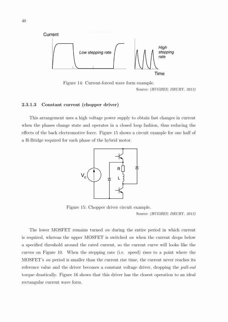
2.3.1.3 Constant current (chopper driver)

This arrangement uses a high voltage power supply to obtain fast changes in current

when the phases change state and operates in a closed loop fashion, thus reducing the

effects of the back electromotive force. Figure 15 shows a circuit example for one half of

a H-Bridge required for each phase of the hybrid motor.

Figure 15: Chopper driver circuit example.


The lower MOSFET remains turned on during the entire period in which current

is required, whereas the upper MOSFET is switched on when the current drops below

a specified threshold around the rated current, so the current curve will looks like the

curves on Figure 10. When the stepping rate (i.e. speed) rises to a point where the

MOSFET’s on period is smaller than the current rise time, the current never reaches its

reference value and the driver becomes a constant voltage driver, dropping the pull-out

torque drastically. Figure 16 shows that this driver has the closest operation to an ideal

rectangular current wave form.

41

Figure 16: Chopper driver wave form example.


The three driver types explained previously show that step motors always tend to

never reach the rated current when the stepping rate rises to the points where the on

period of the driver is smaller than the L/R time constant of the motor, thus leading to

a rapid descend in the pull-out torque delivered by the rotor.

This is the reason why step motors torque drops as speed rises, and this TorqueXSpeed

curve depends on the motor, the driver, the excitation mode and the power supply. It

is not a closed formula and is usually presented in the data sheets on a limited number

of tested parameters, that is, the manufacturers do not present this information with

sufficient data, so costumers do not have many options to work with when designing an

application. For example, Figure 17 shows the TorqueXSpeed curve for the motor model

KTC-HT34-487, where the manufacturer shows two curves for different stepping rate val-

ues, but does not say, however, at which voltage these curves where obtained (usually for

NEMA34 size motors, the voltage is 24/48 V DC, but it is not guaranteed). Another ex-

ample, from the same manufacturer, is the motor model KTC-110HS165, shown in Figure

18, where the voltage is specified as 80 V DC, however no micro stepping rate information

is given.

Figure 17: TorqueXSpeed curve for the motor KTC-HT34-487.

Source: Kalatec c©

42

Figure 18: TorqueXSpeed curve for the motor KTC-110HS165.

Source: Kalatec c©

These inconsistencies in step motor manufacturers data sheets, makes it difficult to

arrive at a precise conclusion upon specification, specially because it is not possible to

guarantee, from the documentation available, the torque of a given motor at the desired

speed for the application, given all the application operation conditions, such as: supply

voltage, rated current, micro stepping rate, load torque and speed.

2.4 The γ factor

To choose the step motor for an application one must consider its TorqueXSpeed

limitations. The motor can stall and loose synchronism due to disturbances or a change

in the load’s torque, for example. To overcome this problem, one must select a motor

with higher torque. The question is: how much higher?

The γ factor is used to quantify the previous question and is in practice greater than

one. It regulates the maximum torque that needs to be delivered by the motor, specifying

a new requirement to motor selection. Defining τf as the torque needed to move the load

and τm the torque of the motor, Equation 2.6 gives the new value to be pursued when

selecting the motor:

τm = γτf . (2.6)

43

2.5 Step motor selection

Several technical features need to be considered in the process that will result in the

right step motor for the application: i) Driver selection, ii) Programming platform (PLC

x Microcontroller), iii) Physical space, iv) Total cost, v) Speed x Torque. The correct

choice will provide a system that delivers the maximum torque, without overloading and

preserving its full lifetime. In the following, we present the criteria used to select the

driver and the gearbox.

2.5.1 Driver selection

When using an encoder to read the position feedback from the axis in a system with

gearbox, it is necessary to compare the encoder’s resolution and the backlash (i.e. the

gap between mechanical parts of a system in which one part moves towards the next

without applying force to it) from the gearbox. If the encoder resolution is higher than

the backlash, the closed loop system will naturally try to compensate the backlash all the

time, wasting power to perform an error correction that can not be accomplished, due to

the system’s dynamics. To avoid this, one should first estimate the gearbox backlash and

either select an encoder with lower resolution or include a minimum error tolerance in the

controller before it actuates.

According to Equations 2.1 and 2.2, the higher the current on the windings, the higher

the torque, and the higher the supply voltage, the higher is the torque (Geckodrive Motor

Controls (GMC), 2010). On the case study presented in this work, the driver selected

is a PCB (Printed Circuit Board) driver with external power MOSFETs, and a 48 VDC

supply voltage.

2.5.2 Gearbox selection

The gearbox is a resource widely used by many applications, as it multiplies the torque

on the shaft. But to achieve this, it imposes a speed reduction on the motor. The gearbox

reduction rate is defined in Equation 2.7:

η =ωmωf, (2.7)

where ωm is the speed of the motor and ωf is the desired speed.

The gearbox chosen for this case study is a worm gearbox type, as shown in Figure

44

19, with speed reduction of 1 : 7.5, meaning that the motor must run 7.5 times faster to

achieve the desired speed. The backlash of the gearbox, which stands for how much the

input axis will move before the engines inside the gearbox actually touches the next teeth

and produce movement to output shaft, is 45 arcmin ≡ 0.75o, which is less than the

output’s resolution of 1.8o/step, in order to not generate a pulse at the encoder when the

backlash is at its maximum.

Figure 19: Worm gearbox detail.

Source: DEV O GearDrive c©

2.5.3 Step-by-step guide of step motor selection

Figure 20 shows an example of a TorqueXSpeed curve for the motor 86HS82 −4504A14−B35−02 (by Policomp c©). The given curve was obtained by the manufacturer

using a 48 VDC power source, 4.45 A current, and 1/8 micro stepping configuration. Since

the curve presented by the manufacturer is obtained empirically under different operating

conditions, it would be impractical to precisely estimate the Torque× Speed relation to

the desired operating conditions for each candidate motor.

To find the motor that fits the requirements, one should essentially estimate the motor

curve on the desired operation conditions and verify whether the selected motor has the

required torque at the required final speed. In order to select the motor-gearbox setup,

Equation 2.8 must be satisfied:

45

Figure 20: TorqueXSpeed graph of the step motor 86HS82-4504A14-B35-02Source: The author

τmη > γτf . (2.8)

where τm is the torque of the motor, τf is the required torque to the axis, η is defined in

Equation 2.7, and γ is defined in Equation 2.6. The value of γ must be either 1.3 or 1.5

(those values are explained in the following). If Equation 2.8 is not satisfied, the setup

must be changed. The γ factor is imperative to establish robustness of the application.

The author proposes a linear estimation for voltage supply starting from the provided

curve and then multiplied by a factor γ = 1.3 (this value is encouraged to be used with a

closed loop. If the system works in open loop, the authors recommend a value of γ = 1.5).

The value γ = 1.3 has been validated in practice to be a good choice for this application.

This factor is to perform secure operation without stalling the motor during the process,

because if γ = 1 is chosen and the motor stalls, even with an feedback system, and if

the machine is operating within unusual conditions, the controller might not be able to

prevent unstable behaviour.

Most of manufactures provide only one graph for each motor, and to arrive in a

consensus of what motor to choose, estimations need to be made based on the information

given in the data sheets. For example, the behaviour of the Torque × Speed curve with

a different power supply has direct influence on the output torque and power delivered

by the motor (Geckodrive Motor Controls (GMC), 2010). These estimations need to be

done very carefully, since motor performance changes from one driver to another, as well

as with other parameters, such as resonance and inertia (users.ece.utexas.edu, 2000).

46

We propose a step-by-step guide to select a step motor for a given application:

1. Calculate the torque needed on the axis, τf ;

2. Define technology (PLC or microcontroller) to be used on the project;

3. If the system will operate in closed-loop, with position feedback from an encoder,

then go to 4. If the system is open-loop, then go to 5;

4. Define γ = 1.3, then go to 6;

5. Define γ = 1.5, then go to 6;

6. Estimate the maximum speed of operation;

7. Select a step motor and/or a gearbox, and calculate τm by using the speed× torquegraph (like in Figure 20).

8. If Equation 2.8 is met, then go to 10, else go to 9

9. Compare the speed X torque curve of the motor with the relations available for the

chosen gearbox and evaluate if the motor, the gearbox or both should be changed,

then go back to 7.

10. Test the motor/gearbox setup on site and verify whether all the necessary variables

were considered in step 1. If the test is successful, then the process is complete,

otherwise go to 1.

The process of estimating the behaviour of the motor is a trial and error process

(users.ece.utexas.edu, 2000). The author proposes that the designers consider a linear

relation from the manufacturer’s information when varying the parameters within a small

range and start the trial process. This range, however can vary within the same motor

under different operation conditions.

47

3 THE ROBOTIC ARM

This chapter presents the mathematical model for the 1 DOF robotic

arm analysed in this work together with an equilibrium analysis.

3.1 Equations of the arm

The arm’s dynamic equations are derived below, as shown in Figure 21. Considering

a rigid body of length L1 with a mass mg concentrated at the tip, θ1 the angle measured

from the horizontal axis (x axis) and the base of the body as the reference frame origin, the

end effector coordinates in function of the joint coordinate are presented in Equation 3.1.

Differentiating it in relation to time, we find the velocity vector, described in Equation

3.2.

Figure 21: Robotic arm.

Source: The author

48

x1(t) = L1cos(θ1(t)),

y1(t) = L1sin(θ1(t)),(3.1)

x1(t) = −θ1(t)L1sin(θ1(t)),

y1(t) = θ1(t)L1cos(θ1(t)),

v(t) =

[x1(t)

y1(t)

].

(3.2)

The velocity vector can be squared, as shown in Equation 3.3, and then used to

calculate the systems kinetic energy in Equation 3.4:

v(t)2 = ||v(t)||2 = v(t)Tv(t) =[−θ1(t)L1sin(θ1(t)) θ1(t)L1cos(θ1(t))

] [−θ1(t)L1sin(θ1(t))

θ1(t)L1cos(θ1(t))

]= θ1

2(t)L2

1,

(3.3)

K =1

2mv2 =

1

2mgθ1

2(t)L2

1. (3.4)

The potential energy is shown in Equation 3.5:

U = mgh = mggL1sin(θ1(t)). (3.5)

Both potential and kinetic energies are used to calculate the Lagrangian defined in

Equation 3.6:

L = K − U =1

2mgθ1

2(t)L2

1 −mggL1sin(θ1(t)), (3.6)

and used in the Euler-Lagrange equation to calculate the load torque τL of the arm, as in

Equation 3.7 (SPONG; HUTCHINSON; VIDYASAGAR, 2005):

τL =d

dt

∂L

∂θ1

− ∂L

∂θ,

τL = θ1mgL21 −mggL1cos(θ1(t)).

(3.7)

Equation 3.7 shows that the torque exerted by the arm depends on the inertia of the

49

arm as a rigid body and on a sinusoidal term, meaning that the load torque depends on

the arm’s position. It can also de used to calculate the maximum torque required to move

the load from rest (when the arm is not carrying any load)):

τL = ��:0

θ1mgL21 −mggL1��

��:1cos(θ1) , τL = −mggL1 = 1.4024 Nm, (3.8)

where:

• mg = 0.530kg

• L1 = 0.270m

• g = 9.8m/s2

Equation 3.8 can be used as the τf value described in step one of section 2.5.3, by

adding an estimation of the heaviest coconut to the the value of mg.

3.2 Mathematical model for the complete mechanical

system

The torque of the step motor, τm, must be equal to or greater than the load torque

in order for the system to move, from which one can derive Equation 3.9.

τm = θ1mgL21 −mggL1cos(θ1(t)) +Bθ1(t). (3.9)

Combining Equation 3.9 of motion and Equation 2.5 of the step motor, a state space

model with four state variables can be derived to represent the system in the continuous

time domain. This combination is straight forward in this approach since the angle of the

arm is the same as the angle of the motor shaft, that is, θ1 = θm.

Electing the state variables as: i) x1(t) = θ1(t), the arm’s angle, ii) x2 = θ1(t) the

arm’s speed, iii) x3(t) = ia(t), current on phase “A” and iv) x4(t) = ib(t), current on

phase “B”, the combined equations written in form of state variables are presented in

Equation 3.10:

50

x1(t) = x2(t),

x2(t) =ψm[−sin(nx1(t))x3(t) + cos(nx1(t))x4(t)] +mggL1cos(x1(t))−Bx2(t)

JL + Jm,

x3(t) =u1(t) + ψmsin(nx1(t))x2(t)−Rx3(t)

L,

x4(t) =u2(t)− ψmcos(nx1(t))x2(t)−Rx4(t)

L,

(3.10)

where:

• Jm is the moment of the inertia of the motor.

• JL is the moment of inertia of the load.

The control inputs are: i) u1(t), voltage on phase “A” and ii) u2(t), voltage on phase

“B” with all states measured, hence the output is y(t) = [x1(t) x2(t) x3(t) x4(t)]. These

equations form a nonlinear system with 4 measured state variables where the main ob-

jective is to control the position and velocity of the arm. The load inertia of the arm is

given by Equation 3.11:

JL = mgL21. (3.11)

The system uses a gearbox as described in section 2.5.2 with ratio 1 : 7.5, applying the

value of η = 7.5 to JL gives the actual moment of inertia J1 felt by the motor, described

in Equation :

J1 =JLη2

=mgL

21

7.52= 0.00068 kgm2. (3.12)

The chosen value of the rotors inertia of the step motor is Jm = 2.7 × 10−4 kgm2,

which represents 39% of the moment inertia J1 sensed by the motor. The total moment

of inertia of the systems is given by Equation 3.13:

Jtot = J1 + Jm. (3.13)

51

3.2.1 Equilibrium analysis

Whereas a complete Step System operates essentially in a discrete manner, the equa-

tions in the continuous time domain are, however, important to perform equilibrium

analysis in order to understand the system’s general behaviour. Considering the left side

of equation 3.10 equal to zero (equilibrium state) and electing the variable ρ as a constant

defined by Equation 3.14:

ρ =mggL1

ψm, (3.14)

one wants to fix three different equilibrium points and starting by analysing state variable

x2(t) from Equation 3.10:

1. x1 = 0o : (position “Unload” from Figure 2)

−��:0sin(0) x3 +��

�:1cos(0) x4 = −ρ��:1

cos(0)

x4 = −ρ,u2 = Rx4 → u2 = −Rρ,u1 = Rx3.

(3.15)

Since only the torque from phase “B” is actuating on the shaft at this position,

x3 = 0 ∴ u1 = 0. Considering the driver is able to maintain constant current, the

voltage (control) needed to hold the arm at θ1 = 0o is u1 = 0 and u2 = Rρ.

2. x1 = 90o :

−��:1

sin(90) x3 +��:0

cos(90) x4 = −ρ��:0

cos(90)

x3 = 0,

u1 = Rx3,

u2 = Rx4.

(3.16)

Only the torque from phase “A” is actuating on the shaft at this position, implying

that x4 = 0 ∴ u2 = 0. The load torque τL = 0, making the current x3 = 0. The

current of both phases “A” and “B” are zero, thus no torque is necessary to hold

the arm at θ1 = 90o, hence u1 = 0 and u2 = 0. This point is the natural equilibrium

point of the system, that is, no control effort is necessary to hold the system at this

state. But it is a unstable equilibrium, and only a closed loop system can transform

this point in a stable equilibrium point.

52

3. x1 = 30o :

��

�:12−sin(30) x3 +��

��:

√3

2cos(30) x4 = −ρ��:

√3

2cos(30)

x3 −√

3x4 =√

3ρ,

u1 = Rx3,

u2 = Rx4.

(3.17)

Considering that the driver is able to maintain constant current, the voltage, on

both phases, necessary to hold the arm at θ1 = 30o is: u1 = Rx3 and u2 = Rx4.

From Equation 3.17, one can generalize that for any given stationary angle, the volt-

ages u1 and u2 are given by:

sin(x1)x3 − cos(x1)x4 = ρcos(x1),

u1 = Rx3,

u2 = Rx4.(3.18)

This analysis is consistent with what one sees in step motors in practice, where it

is possible to maintain the motor stopped at one specific angle by applying the correct

current value in each phase. In the case of a hybrid step motor with a chopper driver, this

state means a high frequency PWM voltage signal controlling the steady state constant

current.

53

4 STEP SYSTEM OPTIMAL OPERATION:

SIMULATION RESULTS

This chapter presents and describes the Simulink c© model used to

perform both closed loop and open loop analysis together with a pro-

posed framework for a generic performance analysis of step systems.

4.1 Driver and hybrid step motor Simulink c© model

Given that the nature of the problem is moving the arm by a given distance within

minimum time, simulations using the power stepper motor tool fromMatLab/Simulink c©

were performed to analyse the system. For better understanding, the author will define

one simulation as each time the Simulink c© model is executed to simulate the arm moving

from a defined initial angle θ0 to a reference angle θref at a given constant speed ω starting

from rest.

To use the power stepper motor module from MatLab/Simulink c©, the user must

provide an input “STEP” signal with values 1 or 0 to determine whether the driver will

energize the motor or not. As long as it receives a pulse of value one, the driver will

make current flow through the windings according to its configuration. The input “DIR”

receives a signal of value 1 or -1 and tells the driver which winding to energize first and

the direction of the current in one of the windings. This will make the motor rotate

counter-clockwise for DIR = 1, or clockwise for DIR = −1. Figure 22 shows de default

power stepper motor diagram when opening the toolbox.

54

Figure 22: Default power stepper motor module diagram.

Source: MatLab c©

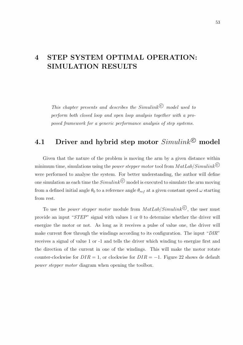
4.1.1 The driver module

The driver module accepts a input DC voltage source input, which configures the

power supply. It is detailed in Figures 23 and 24, respectively, for the default module and

the modified module, used in the closed loop simulations. The highlighted square shows

the part of the block that was modified. The driver needed modifications due to the

fact that the default block is built for only one speed set up through a single simulation,

whereas for the closed loop simulations described in section 4.3 there was the need to

change the speed of the motor (e.g, the drivers pulse rate) in a single simulation.

The highlighted square in Figure 23 shows the part of the block that builds the

excitation signal frequency (defined by the parameter “pulse rate” of the driver block)

and amplitude according to the desired speed and micro stepping rate (i.e, in this case

1600 PPR). This will be later multiplied by two lookup tables, one for each phase of

the motor, and then weighted by the reference current to define the excitation sequence

through time. This excitation signal will define for how long the reference current will

stay in a certain level, obeying the desired micro stepping rate, so the current will behave

as in Figure 10.

55

Figure 23: Default driver module diagram.

Source: The author

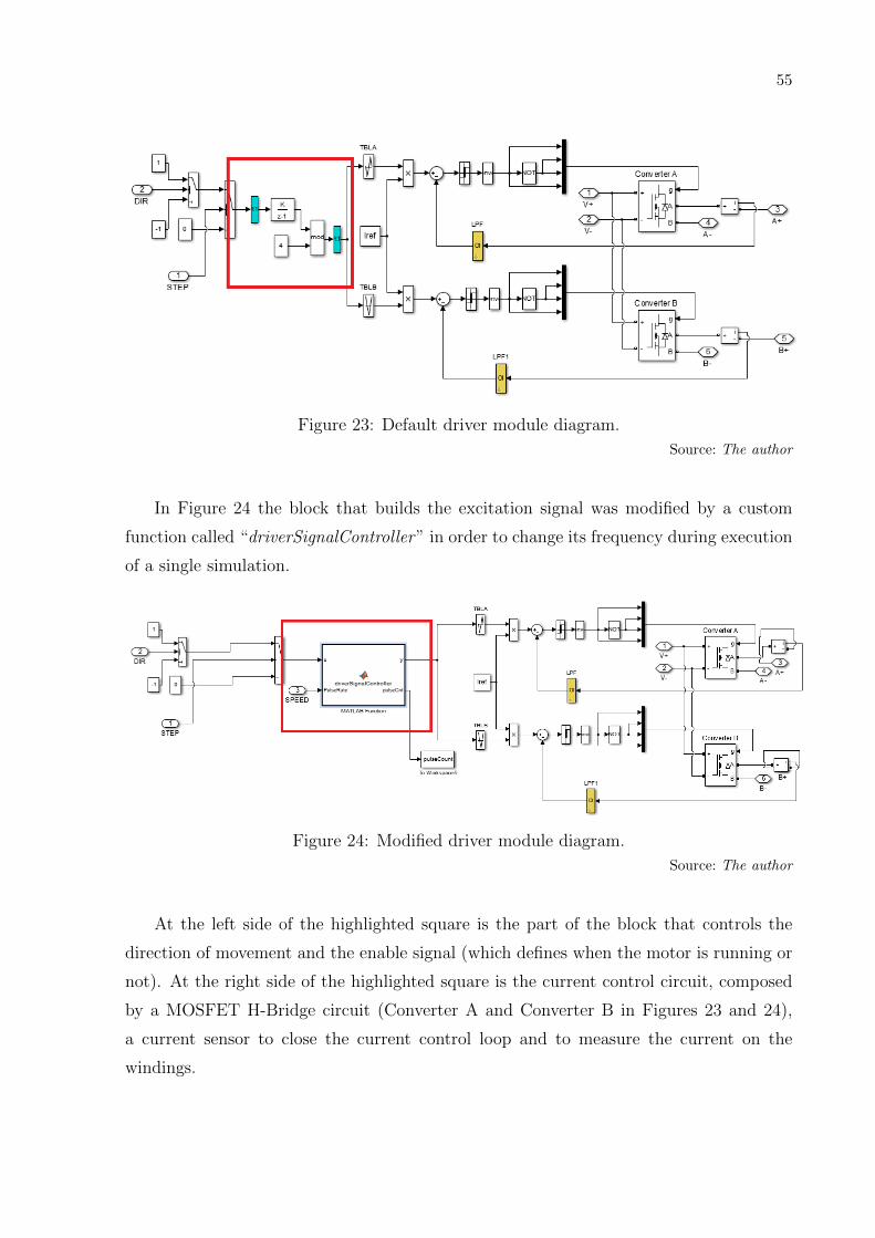
In Figure 24 the block that builds the excitation signal was modified by a custom

function called “driverSignalController” in order to change its frequency during execution

of a single simulation.

Figure 24: Modified driver module diagram.

Source: The author

At the left side of the highlighted square is the part of the block that controls the

direction of movement and the enable signal (which defines when the motor is running or

not). At the right side of the highlighted square is the current control circuit, composed

by a MOSFET H-Bridge circuit (Converter A and Converter B in Figures 23 and 24),

a current sensor to close the current control loop and to measure the current on the

windings.

56

4.1.2 The motor module

The power stepper motor module implements the step motors equations described in

section 2.2. Figure 25 shows the 3 main blocks of the model:: i) Windings, ii) Mechanical

and iii) EMF (electromotive force).

Figure 25: Diagram of the motor’s module.

Source: Simulink c©

Figure 26 details the block diagrams for the main blocks of the hybrid motor module

presented in Figure 25:

57

(a) Diagram of the motor’s module windings block diagram.

(b) Diagram of the motor’s module mechanical blockdiagram.

(c) Diagram of the motor’s module EMF block diagram.

Figure 26: Details of the motor’s module.

Source: Simulink c©

One can note that these blocks implement the motor’s Equations 2.1, 2.2 and 2.3

and 2.5, thus ensuring that analysing the simulations results corresponds to analysing

the desired behaviour of the model presented in this work using a chopper driver (section

2.3).

4.2 Open loop scenario

The open loop simulations consist of defining an initial angle θ0 and a target angle

θref , the pulse rate (i.e speed) and the maximum current. Then calculate the direction

of the movement and the number of pulses, Np, necessary to run the desired distance

based on the selected micro stepping rate, which is a straightforward calculation, shown

in Equation 4.1:

58

Np =|∆θ|PPR

(4.1)

Finally, calculate the simulation time, tsim, that is the duration time for the Simulink c©

model to run. It is important to calculate this time in order to change it from one simula-

tion to another when performing several simulations for different speeds ω. The simulation

time is given by Equation 4.2:

tsim =Np

ω(4.2)

The toolbox provides the feature for defining an initial speed. This feature was used

for the open loop simulations, in order to simplify the system at first, so an acceleration

ramp for departing the motor from rest was not implemented. It is done for the closed

loop simulations scenario, instead the initial speed is define as ω for each selected value

of ω.

Each simulation provides a visualization of the angle through time. Figure 27 shows an

example of a simulation from θm = 0o to θm = 30o at a constant speed of ω = 1.1781rad/s.

This simulation in particular has an execution time greater than necessary in theory, to

acquire data for analysing the behaviour of the windings voltage and current at non-

zero current and non-zero load condition (e.g., the motor is static holding the load at

θm = 30o).

time (10µs)×104

0 1 2 3 4 5 6 7 8 9

θm

(º)

0

5

10

15

20

25

30

35Angle x Time ( ω = 1.1781rad/s)

Figure 27: Angle output of one simulation from the power stepper motor module.

59

From this information, one can extract the value of the angle at the desired sample

time. Sampling the angle at the specified pulse time and taking the difference between

one sample to the next will result in the actual displacement between command pulses,

δθ∗ defined in Equation 4.3.

δθ∗(n) = θ1(n)− θ1(n− 1), ∀ n = 1, 2, ...Np. (4.3)

In an ideal scenario, δθ∗ is constant and equal to the programmed step angle δθ. This

however is not what happens in practice, where δθ∗ presents small variations from δθref .

In order to evaluate how far from δθref (i.e, the configured micro stepping) the system is

when performing a displacement of ∆θ, it is proposed to evaluate the mean of the actual

displacement δθ∗, define in Equation 4.4. This mean will give a single value at the end of

the movement to evaluate if the system lost steps or not:

µδθ =1

Np

Np∑n=1

δθ∗(n). (4.4)

Figure 28 shows the actual step angle taken by the motor through time. It is clear

that there is an overshoot at the beginning due to inertia acceleration. However the motor

tends to maintain an average step angle of µδθ = 0.2254o.

time (10µs)0 100 200 300 400 500 600 700 800

step

Ang

le (

º)

-0.1

0

0.1

0.2

0.3

0.4

0.5Step Angle " θ

Figure 28: Step angle δθ output of one simulation from the power stepper motor module.

Source: The author

60

The mean of the difference µδθ, which represents the average distance travelled by the

motor between command pulses, should be equal to the programmed δθ in an ideal sce-

nario. When this mean starts to deviate from the reference value of δθ (i.e, the configured

micro stepping rate, in this case δθref = 0.2250o), it indicates that the motor is loosing

steps. In other words, the rotor is not moving the distance that it is supposed to move

between command pulses.

To evaluate the effectiveness of the motor in the system, several simulations were

performed at different speeds ω (rad/s) resulting in curves like the one in a Figure 29.

When ω > 2.0rad/s the mean step angle µδθ starts to deviates from the programmed step

angle δθ = 0.2250o.

Speed (rad/s)1 2 3 4 5 6 7 8 9 10

Mea

n S

tepA

ngle

(º)

0

0.2

0.4

0.6

0.8

1

1.2

1.4

1.6

1.8

2

30 = 0 | 3

ref =30 | " 3 =-30 | PPR = 1600 | m = 0.53Kg

Figure 29: Average step angle µδθ for several simulations at different speeds and the samereference angle θref .

Source: The author

Analysing the speed range of 2.4 6 ω 6 3.6, approximately, gives the idea that the

motor does loose steps, but does not necessarily enters a unstable state (i.e, when the

system stops responding to command pulses), which is possible by closing the loop, so

the system tends to become more robust and might be able to run at higher speeds.

Specific studies should be done, but the completeness of this scenario suggests that an

improvement is possible. This improvement is one of the main advantages of closing the

loop of an usually open-looped system, allowing the use of a step motor in high speed and

medium torque applications.

61

Plotting this curve for different target angles θref results in a surface plot where

one can evaluate the influence of the travelled distance on the unstable behaviour of

the system. Figure 30 shows three different surfaces for three different initial angles θ0

resulted from simulations with mg = 0.530 kg, PPR = 1600 and Iref = 6A, which is the

reference current for the driver. Several simulations for different stationary speeds, ω, are

performed for each value of θref in the interval [0o,90o].

The first and expected observation is that for high speeds (ω > 2 rad/s) the motor

starts to loose steps and the mean stepped angle, µδθ , tends to zero. In another words,

the motor tends to not move and starts to present an oscillatory behaviour. Another

observation is that for θ0 = 45o the mean stepped angled around θ0 deviates a little from

the reference even for low speeds.

62

020

40θ

ref60

80

θo = 0 | PPR = 1600 | m = 0.53Kg

987ω (rad/s)6543210

0.2

0.15

0.1

0.25

0

0.05

µ∆θ

X: 90Y: 1.963Z: 0.2256

(a) θ0 = 0o

020

40θ

ref60

80

θo = 45 | PPR = 1600 | m = 0.53Kg

987ω (rad/s)6543210

0.2

0.15

0.1

0.05

0

0.25

µ∆θ

(b) θ0 = 45o

020

40θ

ref60

80

θo = 90 | PPR = 1600 | m = 0.53Kg

987ω (rad/s)6543210

0.1

0.15

0

0.05

0.25

0.2

µ∆θ

(c) θ0 = 90o

Figure 30: Surfaces plot for three different initial angles.

Source: The Author

63

In open loop, in order to reach the desired angular position, one must operate the

motor in the ”plato” region of the surfaces in Figure 30a. The number of steps must be

calculated in order to achieve the final position and applied to the driver.

4.3 Closed loop scenario

In closed loop form, which allows the operation in higher velocities (that is, when the

surface is ”falling” in Figure 30a, 30b and 30c), one can extend the possibilities of using

the step motor in an application. Position feedback is used to track the position error

and design a controller that sends pulses to the driver while the error does not reach a

desired threshold, meaning that the number of pulses is no longer constant. This approach

implies the need for a safety measure in case the step motor stalls, so the controller must

monitor the trajectory evolution and detect a stall situation in order to stop the motor.

For simplicity, this safety measure won’t be covered in this work.

4.3.1 Description

The closed loop system operates using a controller that controls the position of the

arm using the output angle error e(θ1) to adjust the speed in order to achieve the desired

position at minimum time. Figure 31 shows the block diagram for the closed loop system.

The idea to use position feedback to directly actuate in the speed of the motor comes

from the fact that, for this case, when the arm approaches the desired position, the P

controller automatically starts to decrease the speed of the motor, so no additional break

system is necessary.

P Driver Step motor Armω ua,b τem

Encoder

θ1ref e(θ1) θ1−

θ1

Figure 31: Block diagram of the closed loop system.

Source: The author

For the purpose of this work, which is to analyse the behaviour of the complete system,

combining the actuator and motor models together, a simple proportional controller with

gain of P = 100 was chosen to evaluate this case study and to formulate the framework

64

described in the next section. However, more advanced versions of this controller should

be an object of study for further works. In practice, the step motor needs an acceleration

ramp to depart from rest and cannot change speed drastically, in order to ensure a smooth

movement and preserve the mechanics of the system. Therefore, the motor’s acceleration

and the controller’s frequency of actuation were predefined to simplify the analysis. Figure

32 shows the modified Simulink c© model.

Figure 32: Modified Simulink c© model.

Source: The author

The modified Simulink c© model presents the following extra components:

• microController: A Matlab c© function block that implements the micro controller

functions that reads the encoder signal, calculates de error e(θ1) and sends it to the

Discrete PID controller block. It also controls the STEP and DIR inputs of the

driver and sets a flag when the motors stops, that is used by the mass estimation

block.

• speedRamp: A Matlab c© function block that implements the acceleration ramp

when the motor starts from rest and sets the upper limit for the PID controller

block.

• Load 1: This block implements the load torque τL equation as an input into the

hybrid step motor block.

• Mass Esimation: This block implements the mass estimation, detailed in section

5.2.

65

Once the motor is accelerated, ideally, the controller should be free to achieve a

maximum speed. This idea, however, is not straightforward when it comes to step motors,

due to the Speed X Torque trade-off mentioned in chapter 2. As the speed goes high, the

torque diminishes and the motor will no longer respond to the desired micro stepping

configuration, therefore µδθ → 0, which means that for every command pulse, at high

speeds, the motor will only perform a fraction of the configured δθ.

The controller needs a saturation value, ωmax, to ensure that the motor will not

increase the speed indefinitely, leading to a loss of synchronism. In this scenario the

saturation speed ωmax (i.e, the maximum speed of the system) is defined as the maximum

speed the controller will allow the system to run, to travel the distance between any given

initial angle θ1ini and the target position θ1ref , defined as ∆θ1. The time taken to go

through ∆θ1 is defined as ∆t1 = t1 − t0.

4.3.2 Examples

To illustrate this behaviour, we will show in the following the simulations of the

angle θ1(t), speed ω(t), current I(t) and controller output PPSref (t) for three different

saturation speeds: ωmax ∈ [0.9817, 2.3561, 3.5343] and θref = 135o. Figures 33, 34 and

35 show, respectively, simulation results for ωmax = 0.9817 rad/s, ωmax = 2.3561 rad/s

and ωmax = 3.5343 rad/s. It is possible to note that for ωmax = 2.3561 the system

starts to loose steps, but the time ∆t1 is smaller than for ωmax = 0.9817. However for

ωmax = 3.5343, ∆t1 ≈ 1.9 s, which is higher than ∆t1 ≈ 1.175 s for ωmax = 2.3562, and

one can note that the step loss is more significant and more notable at the angle profile.

Figure 36 shows the same results for the case where the P controller has no upper

saturation limit. In another words, ωmax is not defined and the controller is free to increase

the pulse frequency, PPSref , sent to the driver. For this situation, it is important to notice

that the motor does not move forward after 0.8 s, keeping still at θ1 = 25o, which is the

main reason because the controller needs a saturation speed ωmax.

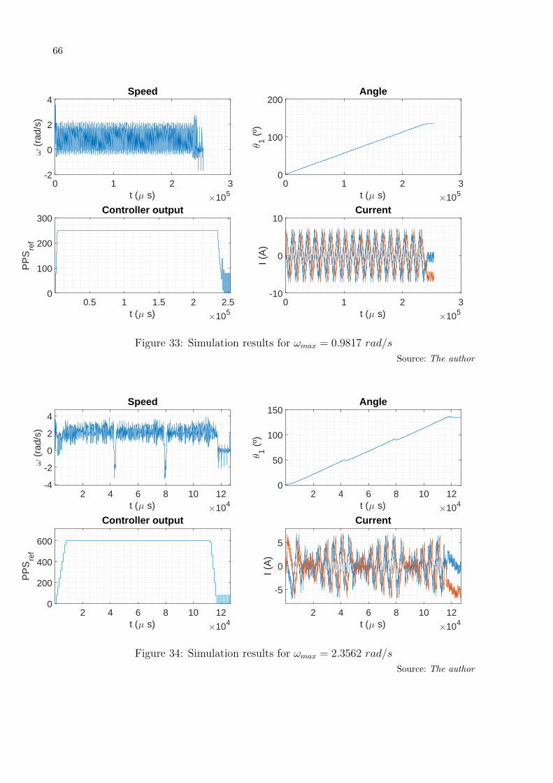
66

t (µ s)×105

0 1 2 3

ω (

rad/

s)

-2

0

2

4Speed

t (µ s)×105

0 1 2 3

θ1 (

º)

0

100

200Angle

t (µ s)×105

0.5 1 1.5 2 2.5

PP

Sre

f

0

100

200

300Controller output

t (µ s)×105

0 1 2 3

I (A

)

-10

0

10Current

Figure 33: Simulation results for ωmax = 0.9817 rad/s

Source: The author

t (µ s)×104

2 4 6 8 10 12

ω (

rad/

s)

-4

-2

0

2

4

Speed

t (µ s)×104

2 4 6 8 10 12

θ1 (

º)

0

50

100

150Angle

t (µ s)×104

2 4 6 8 10 12

PP

Sre

f

0

200

400

600

Controller output

t (µ s)×104

2 4 6 8 10 12

I (A

)

-5

0

5

Current


Source: The author

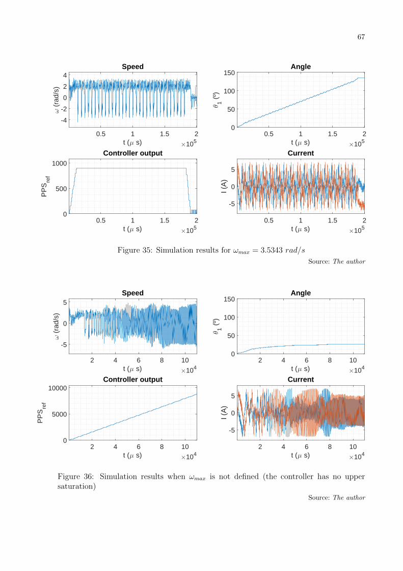
67

t (µ s)×105

0.5 1 1.5 2

ω (

rad/

s)

-4

-2

0

2

4Speed

t (µ s)×105

0.5 1 1.5 2

θ1 (

º)

0

50

100

150Angle

t (µ s)×105

0.5 1 1.5 2

PP

Sre

f

0

500

1000

Controller output

t (µ s)×105

0.5 1 1.5 2I (

A)

-5

0

5

Current


Source: The author

t (µ s)×104

2 4 6 8 10

ω (

rad/

s)

-5

0

5Speed

t (µ s)×104

2 4 6 8 10

θ1 (

º)

0

50

100

150Angle

t (µ s)×104

2 4 6 8 10

PP

Sre

f

0

5000

10000Controller output

t (µ s)×104

2 4 6 8 10

I (A

)

-5

0

5

Current

Figure 36: Simulation results when ωmax is not defined (the controller has no uppersaturation)

Source: The author

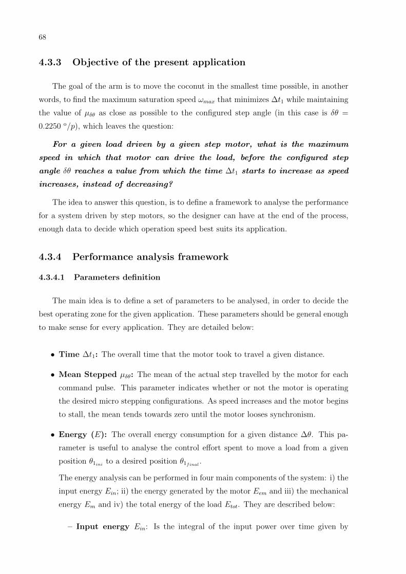
68

4.3.3 Objective of the present application

The goal of the arm is to move the coconut in the smallest time possible, in another

words, to find the maximum saturation speed ωmax that minimizes ∆t1 while maintaining

the value of µδθ as close as possible to the configured step angle (in this case is δθ =

0.2250 o/p), which leaves the question:

For a given load driven by a given step motor, what is the maximum

speed in which that motor can drive the load, before the configured step

angle δθ reaches a value from which the time ∆t1 starts to increase as speed

increases, instead of decreasing?

The idea to answer this question, is to define a framework to analyse the performance

for a system driven by step motors, so the designer can have at the end of the process,

enough data to decide which operation speed best suits its application.

4.3.4 Performance analysis framework

4.3.4.1 Parameters definition

The main idea is to define a set of parameters to be analysed, in order to decide the

best operating zone for the given application. These parameters should be general enough

to make sense for every application. They are detailed below:

• Time ∆t1: The overall time that the motor took to travel a given distance.

• Mean Stepped µδθ: The mean of the actual step travelled by the motor for each

command pulse. This parameter indicates whether or not the motor is operating

the desired micro stepping configurations. As speed increases and the motor begins

to stall, the mean tends towards zero until the motor looses synchronism.

• Energy (E): The overall energy consumption for a given distance ∆θ. This pa-

rameter is useful to analyse the control effort spent to move a load from a given

position θ1ini to a desired position θ1final .

The energy analysis can be performed in four main components of the system: i) the

input energy Ein; ii) the energy generated by the motor Eem and iii) the mechanical

energy Em and iv) the total energy of the load Etot. They are described below:

– Input energy Ein: Is the integral of the input power over time given by

69

Equation 4.5:

Ein =

∫ ∆t1

Pin dt =

∫ ∆t1

VdcIin dt, (4.5)

where Vdc and Iin are, respectively, the voltage and the current of the input

power supply.

– Motor energy Eem: Is the integral of the power delivered to the motor over

time, given by Equation 4.6:

Eem =

∫ ∆t1

Pem dt =

∫ ∆t1

ViIi dt ∀ i = 1, 2, (4.6)

where Vi and Ii are, respectively, the voltage and current at the windings for

each phase, i = 1, 2, of the motor.

– Mechanical energy Em: Is the integral of the power at the output shaft over

time given by Equation 4.7:

Em =

∫ ∆t1

Pm dt =

∫ ∆t1

τemω dt, (4.7)

where τem is the torque delivered by the motor and ω is the output shaft’s

speed.

– Stored energy Estored: Is the integral of the sum of the kinetic and potential

energies, resulting from combining Equations 3.4 and 3.5, shown in Equation

4.8:

Estored = K + U =1

2mgθ1

2(t)L2

1 +mggL1sin(θ1(t)). (4.8)

4.3.4.2 Parameters analysis

From the energy analysis, naturally follows an efficiency analysis, comparing how much

energy is lost in a step motor driven application. The goal here is to separate the energy

analysis, and to study the loss on both the driver system and on the mechanical system

(i.e, the robotic arm). In order to do so, two different efficiency parameters were defined:

i) electric efficiency Effe and ii) mechanical efficiency Effem. The electric efficiency,

defined in Equation 4.9, represents how much energy is lost from the input power source

to the motor, in another words, how much of the input energy is available for the motor

to drive the load:

Effe =EeEin

. (4.9)

70

The mechanical efficiency, defined in Equation 4.10, represents how much energy

delivered by the motor is converted to the output shaft, in another words, it represents

how good a step motor is in converting electrical energy to mechanical energy:

Effem =EmEem

(4.10)

In order to analyse the efficiencies involved in the process and to best visualize the

losses, the author proposes to compare the overall efficiency (electric and mechanical)

with the first parameters defined in the framework, named time ∆t1 and mean stepped

µδθ. Figures 37 and 38 show, respectively, ∆t1 and µδθ on the left y-axis on a dashed line

and, both Effe and Effem plotted together, in function of the maximum speed ωmax,

on the right y-axis. The dotted line represents the mechanical efficiency Effem and the

dot-dashed line represents the electrical efficiency Effe. The vertical solid line marks the

speed in which the minimum time is achieved (considered all the values ωmax simulated),

which is ω∗max = 2.26 rad/s, and the textbox displays the parameter value as well as the

efficiencies values for ω∗max = 2.26 rad/s.

ωmax

0.5 1 1.5 2 2.5 3 3.5 4

∆ t 1 (

s)

1.1

1.6

2.1

2.6

∆θ = 135º | m = 0.53g

Eff

(%)

0

0.2

0.4

0.6

0.8

1

Tmin

= 1.10s

Effe = 90%

Effem

= 52%

Figure 37: Efficiency analysis by time. The blue dashed (∆t1) line should be read with theleft y-axis whereas the yellow dot-dashed (Effe) and black dotted (Effem) lines shouldbe read with the right y-axis (Eff)

Source: The author

71

ωmax

1 1.5 2 2.5 3 3.5

µδθ

0.0730

0.1230

0.1730

0.2230

" θ = 135º | m = 0.53g

Eff

(%)

0.2

0.4

0.6

0.8

1

µδθ

= 0.21º/p

Effe = 90%

Effem

= 52%

Figure 38: Efficiency analysis by mean stepped. The blue dashed (∆t1) line should beread with the left y-axis whereas the yellow dot-dashed (Effe) and black dotted (Effem)lines should be read with the right y-axis (Eff)

Source: The author

First, note that both efficiencies increases as speed goes higher, Effe from approx-

imately 0.85 to 0.9 and Effem from approximately 0.1 to 0.25. Then the Effe drops

due to the fact that both input energy Ein and the motor energy Eem drop, thus lead-

ing to an increase in the mechanical efficiency Effem. Figure 38 shows that the point

ωmax ≈ 2.26 rad/s is the point where the parameter µδθ starts to drop exponentially,

leading to the time increase seen in Figure 37. It is also the point where minimum time

is achieved and the electrical and mechanical efficiencies are, respectively, Effe = 90%

and Effem = 52%. For ωmax > 2.26 rad/s the time starts to increase and the mechanical

efficiency stabilizes around 45%. This happens due to the fact the the torque of the mo-

tor drops drastically, so an increase in speed will not be converted in a better mechanical

efficiency.

On the contrary, an increase in speed will result in higher friction loss. For the total

energy, it is useful to analyse how much energy is lost when driving the load. Define

the friction energy, Efric as the difference between the mechanical energy and the stored

energy, which is the energy needed to drive the load, as in Equation 4.11::

Efric = Em − Estored. (4.11)

Equation 4.11 shows that the higher the speed, which increases Em, the higher will be the

energy lost in the process. This loss depends only on the speed of the application, which

will reflect on the mechanical system that will have to dissipate this energy. For the arm

presented in this case study, this heat dissipation is not an issue. However it might be an

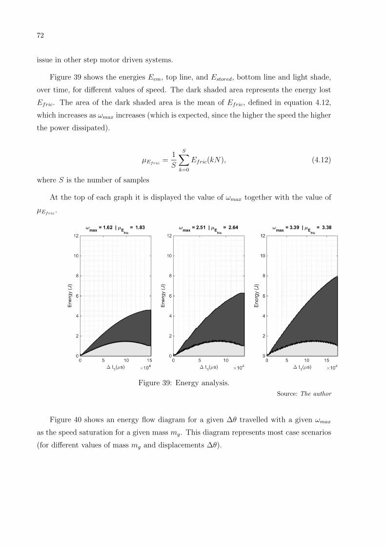
72

issue in other step motor driven systems.

Figure 39 shows the energies Eem, top line, and Estored, bottom line and light shade,

over time, for different values of speed. The dark shaded area represents the energy lost

Efric. The area of the dark shaded area is the mean of Efric, defined in equation 4.12,

which increases as ωmax increases (which is expected, since the higher the speed the higher

the power dissipated).

µEfric =1

S

S∑k=0

Efric(kN), (4.12)

where S is the number of samples

At the top of each graph it is displayed the value of ωmax together with the value of

µEfric .

Figure 39: Energy analysis.

Source: The author

Figure 40 shows an energy flow diagram for a given ∆θ travelled with a given ωmax

as the speed saturation for a given mass mg. This diagram represents most case scenarios

(for different values of mass mg and displacements ∆θ).

73

Figure 40: Energy flow diagram for an operation of the arm.

Source: The author (created with www.sankeyflowshow.com)

74

75

5 LOAD MASS ESTIMATION

This chapter presents the load mass estimation problem together with

the proposed approach to solve it.

5.1 Mass estimation importance

Another important problem in the coconut paring system is the mass estimation. It

was said that the paring process should save the maximum of coconut pulp as possible, and

future additional systems could use the mass information in order to achieve minimum

waste. A precise estimation of the coconut’s mass can also be used to measure of the

performance of the machine without adding an extra step prior to the coconut processing.

With the coconut properly weighed, measuring the machine’s performance is achieved

directly weighting the coconuts after the process, which is simpler and can be done on

batches of several fruits at once. The machine’s performance, ρm, can be defined as the

total weight after the process by the weight before the process, as shown on Equation 5.1.

ρm =wawb. (5.1)

where:

• wb: Is the total weight before the processing.

• wa: Is the total weight after the processing.

This overall performance, depends on several aspects of the operation, such as, the

format and size of the fruits, as well as the speed of the process.

76

5.2 The proposed approach

Since the mass directly affects the load torque τL, as stated in Equation 3.7, the

suggested approach for this scenario is to calculate the motor torque when the arm is

stopped at a given final position θ1. From Equation 3.10, it is possible to isolate the load

torque and the motor torque. Analysing the second state-space equation when the motor

is stopped, it is possible to derive a equation to estimate the mass, which is shown in

Equation 5.2.

x2(t) =ψm[−sin(nx1(t))x3(t) + cos(nx1(t))x4(t)] +mggL1cos(x1(t))−Bx2(t)

Jtot,

��*0

x2(t) =ψm[−sin(nx1(t))x3(t) + cos(nx1(t))x4(t)] +mggL1cos(x1(t))−B��

�* 0

x2(t)

Jtot,

ψm[−sin(nx1(t))x3(t) + cos(nx1(t))x4(t)] = mggL1cos(x1(t)),

mg =ψm[−sin(nx1(t))x3(t) + cos(nx1(t))x4(t)]

gL1cos(x1(t)).

(5.2)

Equation 5.2 is an approximate equation due to the fact that the motor is operated

by a chopper driver controlling the current at high frequencies, which leads to small

variations in current and in the final angle. These variations can be however suppressed

using a moving average filter to filter the high frequencies of the signal and extract a DC

value. The proposed approach is to sample the current and arm angle signals at a sample

period N , resulting in Equation 5.3.

m∗g(kN) =ψm[−sin(nx∗1(kN))x∗3(n) + cos(nx∗1(kN))x∗4(kN)]

gL1cos(x∗1(kN)),∀k = 0, 1, 2 ... N−1. (5.3)

where:

• x∗1(kN): sampled angle;

• x∗3(kN): sampled current from phase A;

• x∗4(kN): sampled current from phase B;

• m∗g(kN): sampled mass signal;

77

After sampled, the values are filtered in real time by a digital moving average window

filter, shown in Equation 5.4:

m∗gavg(kN) =1

W

W∑q=1

m∗g(kN − q), ∀ k > W, (5.4)

where:

• W is the size of the window

• k is the current sample

This approach has the disadvantage of presenting a settling time for the moving

average filter. However, due to the nature of the problem, the arm should remain stopped

at a given position to wait for the paring table. This waiting time presented is sufficient,

since the settling time of the filter turned out to be irrelevant in the simulations performed,

resulting in that the beginning of the signal m∗gavg(kN) can simply be ignored.

To calculate the mass estimation, the system performs a simple mean of a segment of

the signal m∗gavg(kN) from equation 5.4. The estimated mass me is then given by Equation

5.5:

me =1

S

j∑k=i

m∗gavg(kN),∀k = i, i+ 1, i+ 2 ... j, (5.5)

where:

• i and j are the indices that define the interval chosen calculate me, in another words,

i and j define the time span that will be used to estimate the mass.

• j > i

The indices i and j are defined, respectively, by the initial delay ti and the final

measurement time tf , chosen to calculate the mass, and by the sample period N . The

time span of estimation is defined as ∆Tcalc = tf − ti. The number of samples inside

∆Tcalc will, obviously, depend on the sample period N , since the number of samples, S,

is defined as:

S =∆TcalcN

(5.6)

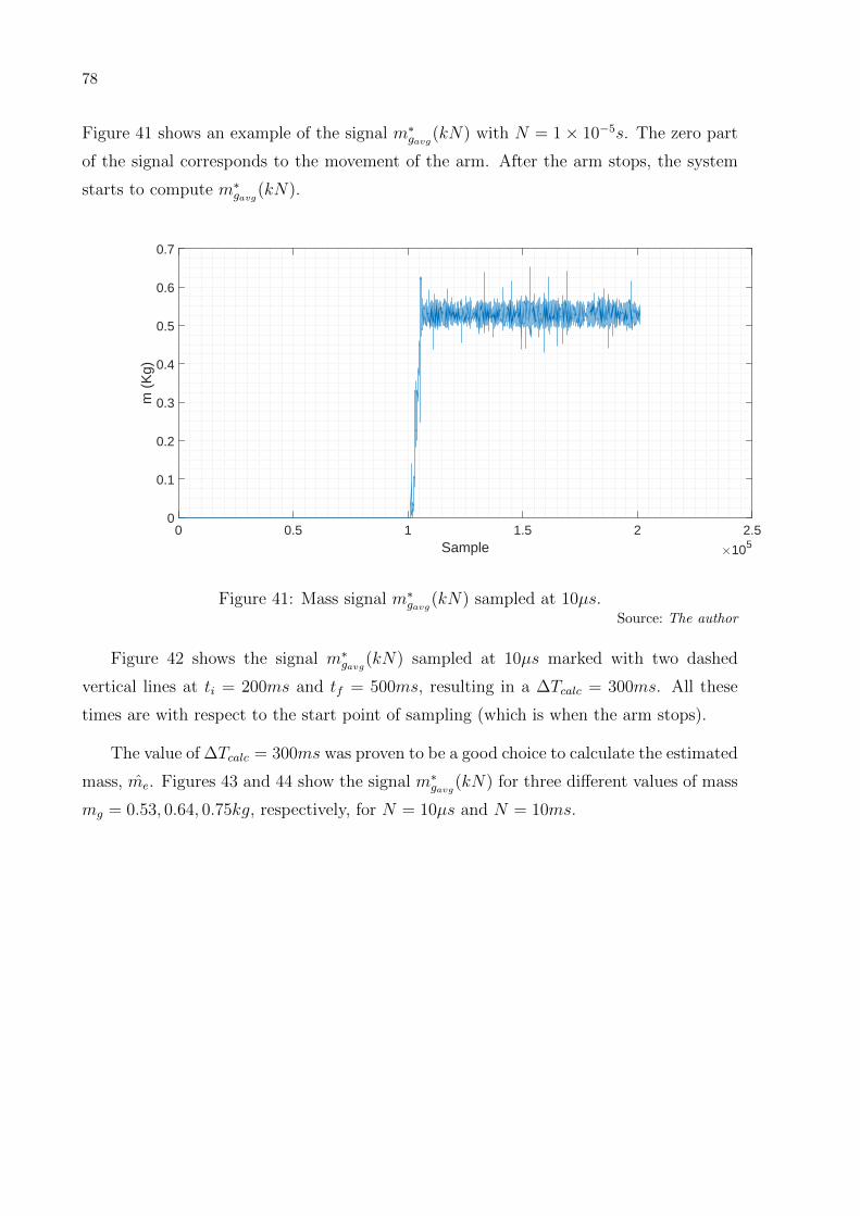
78

Figure 41 shows an example of the signal m∗gavg(kN) with N = 1× 10−5s. The zero part

of the signal corresponds to the movement of the arm. After the arm stops, the system

starts to compute m∗gavg(kN).

Sample ×1050 0.5 1 1.5 2 2.5

m (

Kg)

0

0.1

0.2

0.3

0.4

0.5

0.6

0.7

Figure 41: Mass signal m∗gavg(kN) sampled at 10µs.Source: The author

Figure 42 shows the signal m∗gavg(kN) sampled at 10µs marked with two dashed

vertical lines at ti = 200ms and tf = 500ms, resulting in a ∆Tcalc = 300ms. All these

times are with respect to the start point of sampling (which is when the arm stops).

The value of ∆Tcalc = 300ms was proven to be a good choice to calculate the estimated

mass, me. Figures 43 and 44 show the signal m∗gavg(kN) for three different values of mass

mg = 0.53, 0.64, 0.75kg, respectively, for N = 10µs and N = 10ms.

79

Sample ×1050 0.5 1 1.5 2 2.5

m (

Kg)

0

0.1

0.2

0.3

0.4

0.5

0.6

0.7

Figure 42: Mass signal m∗gavg(kN) sampled at 10ms.Source: The author

Sample ×1050 0.5 1 1.5 2 2.5

m (

Kg)

0

0.1

0.2

0.3

0.4

0.5

0.6

0.7

0.8

0.9N = 1e-05 s

me = 0.53 | m

g = 0.53 (-0.04%)

me = 0.64 | m

g = 0.64 (-0.03%)

me = 0.75 | m

g = 0.75 (-0.04%)

Figure 43: Mass signal m∗gavg(kN) sampled at 10µs for 3 different values of mg.

Source: The author

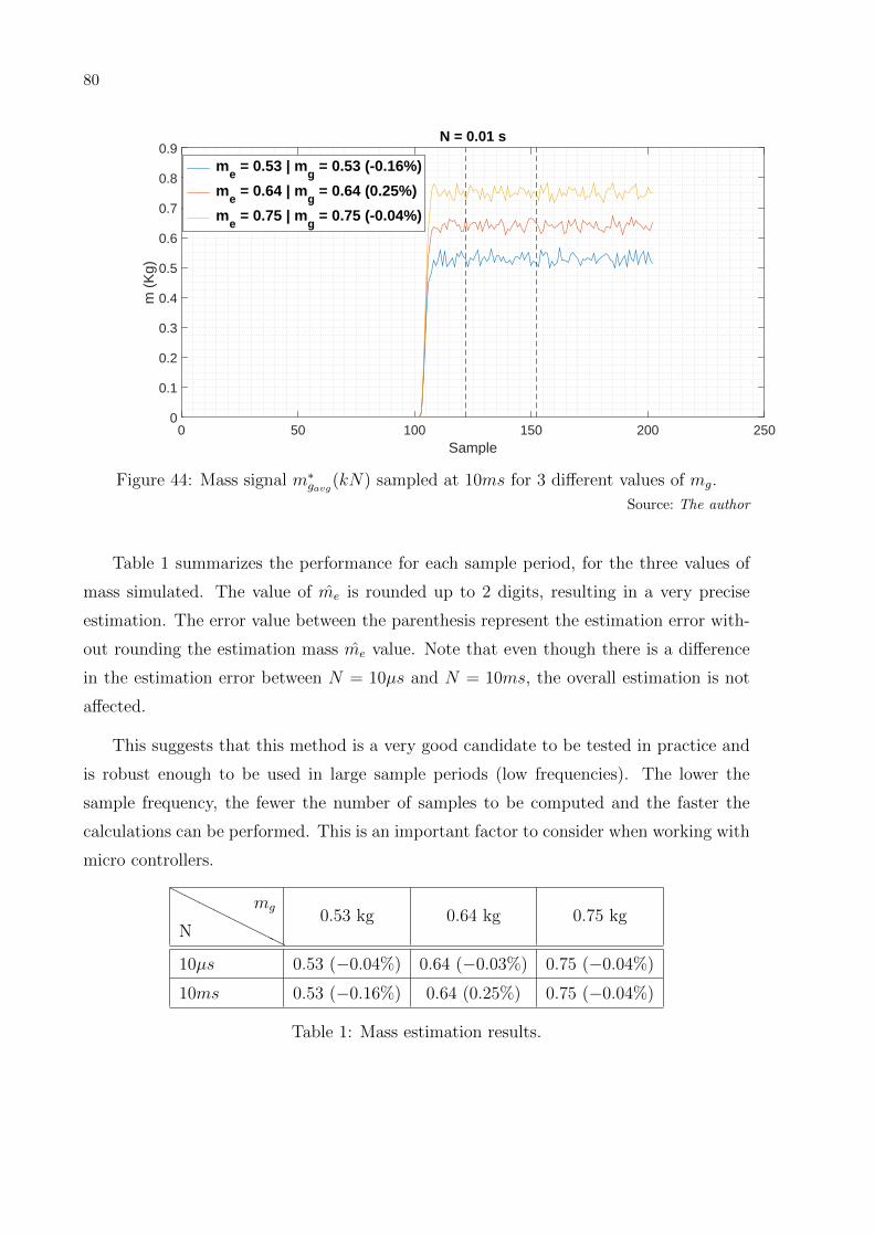
80

Sample0 50 100 150 200 250

m (

Kg)

0

0.1

0.2

0.3

0.4

0.5

0.6

0.7

0.8

0.9N = 0.01 s

me = 0.53 | m

g = 0.53 (-0.16%)

me = 0.64 | m

g = 0.64 (0.25%)

me = 0.75 | m

g = 0.75 (-0.04%)

Figure 44: Mass signal m∗gavg(kN) sampled at 10ms for 3 different values of mg.

Source: The author

Table 1 summarizes the performance for each sample period, for the three values of

mass simulated. The value of me is rounded up to 2 digits, resulting in a very precise

estimation. The error value between the parenthesis represent the estimation error with-

out rounding the estimation mass me value. Note that even though there is a difference

in the estimation error between N = 10µs and N = 10ms, the overall estimation is not

affected.

This suggests that this method is a very good candidate to be tested in practice and

is robust enough to be used in large sample periods (low frequencies). The lower the

sample frequency, the fewer the number of samples to be computed and the faster the

calculations can be performed. This is an important factor to consider when working with

micro controllers.

HHHH

HHHHN

mg0.53 kg 0.64 kg 0.75 kg

10µs 0.53 (−0.04%) 0.64 (−0.03%) 0.75 (−0.04%)

10ms 0.53 (−0.16%) 0.64 (0.25%) 0.75 (−0.04%)

Table 1: Mass estimation results.

81

6 CONCLUSIONS AND FUTURE WORK

This chapter concludes the work by summarizing its main contribu-

tions and identifying possible improvements that can be done in future

works.

A brief review of the main aspects of a step motor was performed and its non linear

mathematical model was presented, as well as combined with a dynamic load model

derived from a 1 DOF robotic arm used to move a coconut from a buffer plate to the

paring table. That is the motivating problem for this work.

This combined model was used to simulate and to study the behaviour of a complete

robotic step system, simulated together with a step driver, thus making the simulations

as close as possible to a practical operation. The model was adapted to work in closed-

loop, which means that some modifications in the built-in Matlab c© driver model were

implemented. This approach allowed a more complete study of an application where the

step motor operates on its limits in terms of speed. The first two main objective of this

work were achieved by the study of the whole step system. The first one was to define

a structured method for selecting a step motor for an application, presented in section

2.5.3. The second one was to formulate a framework to analyse the performance of a

step system according to a set of useful generic parameters: i) time, ii) mean step and

iii) energy consumption, presented in section 4.3.4. Figures 37 and 38 show the first two

parameters as function of the max speed of the system, ωmax, and can be used as a visual

tool to determine the best operating speed. These figures can also be used to validate

that for ωmax greater than the optimal value, the mechanical performance of a step motor

is around 45% for this scenario.

Considering that the complete driver system was simulated, it is enough to say that

the proposed mass estimation approach could be tested in practice to evaluate its per-

formance on the actual machine. Also, the time interval to achieve precision in the mass

estimation was short and simple enough to be implemented in real time and with low

computational burden. The load mass estimation was achieved with high confidence in

82

terms of estimation error, as presented in Table 1, through the analysis of the systems

equation when the arm is stopped at a given position while being excited. Figures 43 and

44 show that the signal obtained by the chosen method is a well behaved signal and can

be used for further practical studies of the problem.

A point of interest is the controller used to set the speed of the motor. Initially

a simple proportional controller was chosen. However, it was noticed in the simulations

that better performance can be achieved when using other controllers, like a PD controller

or a artificial intelligence controller, using fuzzy logic, for example. In (JEONG; LEE;

CHUNG, 2020) the authors present several advanced control methods for permanent

magnet step motors, that can be used as a start point to investigate possible control

schemes for future works.

83

REFERENCES

KHAN, T. A.; TAJ, T. A.; IJAZ, I. Hybrid stepper motor and its controlling techniquesa survey. Proceedings of the 2014 IEEE North West Russia Young Researchers inElectrical and Electronic Engineering Conference, ElConRusNW 2014, p. 79–83, 2014.

HUGHES, A.; DRURY, B. Electric Motors and Drives: Fundamentals, Types andApplications. [S.l.]: Elsevier Science, 2013. ISBN 9780080993683.

HENKE, B. et al. Modeling of hybrid stepper motors for closed loop operation.IFAC, 2013. v. 46. 177–183 p. ISSN 14746670. ISBN 9783902823311. Disponıvel em:〈http://dx.doi.org/10.3182/20130410-3-CN-2034.00042〉.

MORAR, A. The Modelling and Simulation of Bipolar Hybrid Stepping Motor byMatlab/Simulink. Procedia Technology, v. 19, p. 576–583, 2015. ISSN 22120173.

ACARNLEY, P. P.; WATSON, J. F. Review of position-sensorless operation of brushlesspermanent-magnet machines. IEEE Transactions on Industrial Electronics, v. 53, n. 2,p. 352–362, 2006. ISSN 02780046.

DRAAMMELAERE, S. et al. Robust sensorless load angle control for stepping motors.p. 1603–1608, 2015.

LIN, C.; CHEN, P.; CAO, Q. Research on torque-variable control method for steppingmotors in service robot arm. Proceedings of IEEE Workshop on Advanced Robotics andits Social Impacts, ARSO, v. 2016-November, p. 85–90, 2016. ISSN 21627576.

CHUDASAMA, T.; BARIA. Speed and Torque Control of Stepper Motor using Voltageand Current Control. International Journal of Research in Modern Engineering andEmerging Technology, v. 1, n. 3, p. 10–14, 2013.

users.ece.utexas.edu. Stepper motor and driver selection. [ONLINE] Available at: . 2000.http://users.ece.utexas.edu/ valvano/Datasheets/StepperSelection.pdf. [Accessed 25February 2018].

ROBERT, B.; ALIN, C.; GOELDEL, C. Aperiodic and chaotic dynamics in hybridstep motor - New experimental results. IEEE International Symposium on IndustrialElectronics, v. 3, n. May, p. 2136–2141, 2001.

CORRON, N. et al. Eletric step motor non linear dynamics and estimation of theembedding dimension. 2001.

PERA, M.-C.; ROBERT, B.; GOELDEL, C. Nonlinear dynamics in electromechanicalsystems-application to a hybrid stepping motor. v. 7, n. 1, p. 31–42, 2000.

MILADI, Y.; FEKI, M.; DERBEL, N. Using unconventional methods to control thechaotic behavior of switched time systems: Application to a stepper motor. v. 6, n. 4, p.81–89, 2013.

http://dx.doi.org/10.3182/20130410-3-CN-2034.00042

84

LYSHEVSKI, S. E. Microstepping and high-performance control of permanent-magnetstepper motors. Energy Conversion and Management, Elsevier Ltd, v. 85, p. 245–253,2014. ISSN 01968904. Disponıvel em: 〈http://dx.doi.org/10.1016/j.enconman.2014.05.078〉.

Li, P.; Lu, H.; Shen, J. Analysis method of dynamic torque-frequency characteristicof hybrid stepping motors. In: 2017 Twelfth International Conference on EcologicalVehicles and Renewable Energies (EVER). [S.l.: s.n.], 2017. p. 1–6.

Dorin-Mirel, S.; Ion, M.; Mihai, O. The analysis of different frequency for a steppermotor open loop operation. In: 2016 8th International Conference on Electronics,Computers and Artificial Intelligence (ECAI). [S.l.: s.n.], 2016. p. 1–7.

SOUZA, D.; COLoN, D. Step Motor Selection and Control: An Industrial Case Study.Congresso Brasileiro de Automatica CBA2018, 2018. ISSN 25258311.

MELKEBEEK, J. Electrical Machines and Drives: Fundamentals and Advanced Mod-elling. Springer International Publishing, 2018. (Power Systems). ISBN 9783319727301.Disponıvel em: 〈https://books.google.com.br/books?id=G-xHDwAAQBAJ〉.

Dejan Nedelkovski. How a Stepper Motor Works. [ONLINE] Available at: .https://howtomechatronics.com/how-it-works/electrical-engineering/stepper-motor/.[Accessed 12 March 2018].

ACARNLEY, P. Stepping Motors: a guide to theory and practice. [S.l.: s.n.], 2002. ISSN00135127. ISBN 9780852964170.

MORAR, A. Stepper Motor Model for Dynamic Simulation. v. 44, n. 2, p. 117–122,2003.

Mathworks c©. Stepper motor and driver selection. [ONLINE] Available at: . 2007.https://www.mathworks.com/help/physmod/sps/powersys/ref/steppermotor.html.[Accessed 30 June 2020].

George. Unipolar Stepper Motor vs Bipolar Stepper Motors. [ONLINE] Available at:. 2012. https://www.circuitspecialists.com/blog/unipolar-stepper-motor-vs-bipolar-stepper-motors/. [Accessed 12 March 2018].

Derammelaere, S. et al. Torque ripples in stepping motor driven systems. 2015 17thEuropean Conference on Power Electronics and Applications (EPE’15 ECCE-Europe),p. 1–6, 2015.

Geckodrive Motor Controls (GMC). Step motor basics guide. 2010. 1-17 p.

SPONG, M.; HUTCHINSON, S.; VIDYASAGAR, M. Robot Modeling and Control. [S.l.]:Wiley, 2005. ISBN 9780471649908.

JEONG, Y. W.; LEE, Y.; CHUNG, C. A survey of advanced control methods forpermanent magnet stepper motors. In: . [S.l.: s.n.], 2020. p. 331–342.

http://dx.doi.org/10.1016/j.enconman.2014.05.078

http://dx.doi.org/10.1016/j.enconman.2014.05.078

https://books.google.com.br/books?id=G-xHDwAAQBAJ

Documents

ROBOTIC ARM USING STEP MOTORS: STUDIES FOR OPTIMAL