Roberto!A.Bunge AA241X April132015 …adl.stanford.edu/groups/aa241x/wiki/e054d/attachments...Longitudinal & Lateral Decoupling AA241X, April 13 2015, Stanford University Roberto A

Roberto A . Bunge

AA241X

Apr i l 13 2015 S tanford Univers i ty

Aircraft Flight Dynamics

AA241X, April 13 2015, Stanford University Roberto A. Bunge

Overview

1.  Equations of motion ¡  Full Nonlinear EOM ¡  Decoupling of EOM ¡  Simplified Models

2.  Aerodynamics

¡  Dimensionless coefficients ¡  Stability & Control Derivatives

3.  Trim Analysis ¡  Level, climb and glide ¡  Turning maneuver

4.  Linearized Dynamics Analysis ¡  Longitudinal ¡  Lateral


Equations of Motion

�  Dynamical system is defined by a transition function, mapping states & control inputs to future states

Aircraft

EOM

X

δ

!X

!X = f (X,δ)


States and Control Inputs

X =

xyzuvwθφ

ψ

pqr

!

"

#################

$

%

&&&&&&&&&&&&&&&&&

position

velocity

attitude

angular velocity

δ =

δeδtδaδr

!

"

####

$

%

&&&&

elevator

throttle

aileron

rudder


There are alternative ways of defining states and control inputs

Full Nonlinear EOM

�  Dynamics Eqs.* Linear Acceleration = Aero + gravity + Gyro Angular Acceleration = Aero + Gyro

*Assuming calm atmosphere and symmetric aircraft (Neglecting cross-products of inertia

�  Kinematic Eqs.: Relation between position and velocity Relation between attitude and angular velocity

Ixx !p = l + (Iyy − Izz )qrIyy !q =m+ (Izz − Ixx )prIzz !r = n+ (Ixx − Iyy )pq

!x!y!z

!

"

###

$

%

&&&= NRB

(φ,θ ,ψ )

uvw

!

"

###

$

%

&&&

•  System of 12 Nonlinear ODEs

m !u = X −mgsin(θ )+m(rv− qw)m !v =Y +mgsin(φ)cos(θ )+m(pw− ru)m !w = Z +mgcos(φ)cos(θ )+m(qu− pv)

!φ = p+ qsin(φ)tan(θ )+ rcos(φ)tan(θ )!θ = qcos(φ)− rsin(φ)

!ψ = q sin(φ)cos(θ )

+ r cos(φ)cos(θ )


Nonlinearity and Model Uncertainty

�  Sources of nonlinearity: ¡  Trigonometric projections (dependent on attitude) ¡  Gyroscopic effects ¡  Aerodynamics

÷ Dynamic pressure ÷ Reynolds dependencies ÷  Stall & partial separation

�  Model uncertainties: ¡  Gravity & Gyroscopic terms are straightforward, provided we can

measure mass, inertias and attitude accurately

¡  Aerodynamics is harder, especially viscous effects: lifting surface drag, propeller & fuselage aerodynamics


Flight Dynamics and Navigation Decoupling

Roberto A. Bunge AA241X, April 13 2015, Stanford University

Xdyn =

uvwθφ

pqr

!

"

##########

$

%

&&&&&&&&&&

δdyn =

δeδtδaδr

!

"

####

$

%

&&&&

Flight Dynamics

Xnav =

xyzψ

!

"

#####

$

%

&&&&&

δnav =

uvwθφ

pqr

!

"

##########

$

%

&&&&&&&&&&

Navigation

Flight Dyn. δdyn Xdyn = δnav

Nav. Xnav

�  Flight Dynamics is the “inner dynamics” �  Navigation is “outer dynamics”: usually what we care about

The full nonlinear EOMs have a cascade structure

Longitudinal & Lateral Decoupling


�  Although usually used in perturbational (linear) models, many times this decoupling can also be used for nonlinear analysis (e.g. symmetric flight with large vertical motion)

For a symmetric aircraft near a symmetric flight condition, the Flight Dynamics can be further decoupled in two independent parts

Xlon =

uwθ

q

!

"

####

$

%

&&&&

δlon =δeδt

!

"#$

%&

Longitudinal Dynamics

Xlat =

vφ

pr

!

"

####

$

%

&&&&

δlat*=δaδr

!

"#

$

%&

Lateral-Directional Dynamics

* As we shall see, throttle also has effects on the lateral dynamics, but these can be eliminated with appropriate aileron and rudder

Lon.

Lat.

Xlon

Xlat

δlon

δlat

Flight Dynamics

Alternative State Descriptions


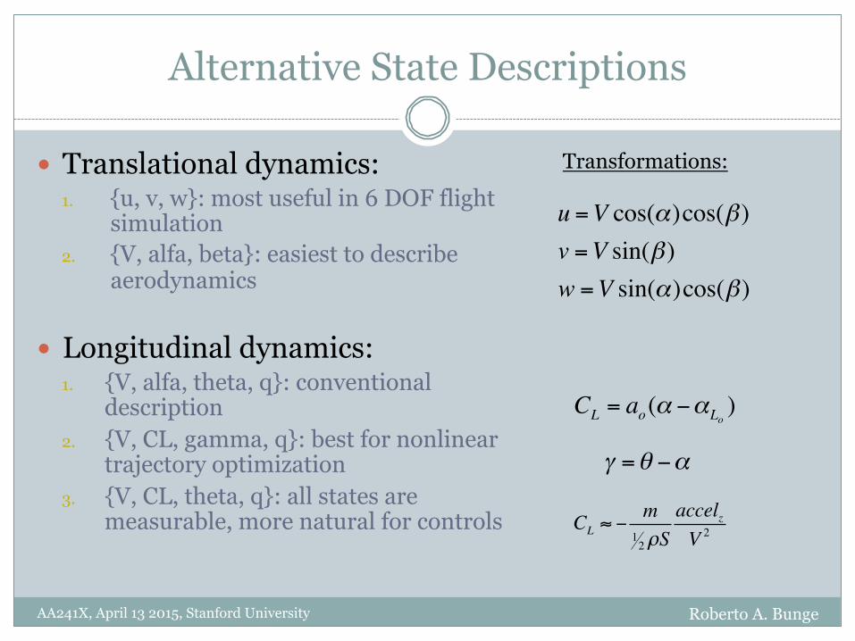
�  Translational dynamics: 1.  {u, v, w}: most useful in 6 DOF flight

simulation 2.  {V, alfa, beta}: easiest to describe

aerodynamics

�  Longitudinal dynamics: 1.  {V, alfa, theta, q}: conventional

description 2.  {V, CL, gamma, q}: best for nonlinear

trajectory optimization 3.  {V, CL, theta, q}: all states are

measurable, more natural for controls

u =V cos(α)cos(β)v =V sin(β)w =V sin(α)cos(β)

CL = ao(α −αLo)

γ =θ −α

Transformations:

CL ≈ −m

12ρS

accelzV 2

Simplified Models


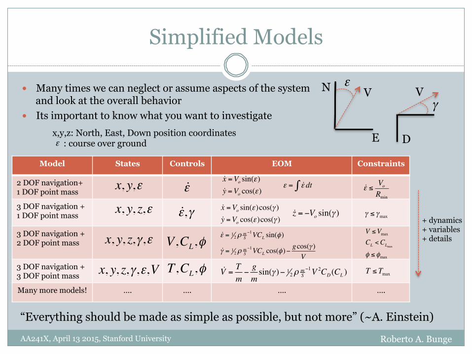
�  Many times we can neglect or assume aspects of the system and look at the overall behavior

�  Its important to know what you want to investigate

Model States Controls EOM Constraints

2 DOF navigation+ 1 DOF point mass

3 DOF navigation + 1 DOF point mass



Many more models! …. …. …. ….

x, y,ε

V N

E

ε

!ε!x =Vo sin(ε)!y =Vo cos(ε)

x, y, z,ε !ε,γ !x =Vo sin(ε)cos(γ )!y =Vo cos(ε)cos(γ )

!z = −Vo sin(γ )

x,y,z: North, East, Down position coordinates : course over ground ε

x, y, z,γ,ε V,CL,φ!ε = 1

2ρ mS−1VCL sin(φ)

!γ = 12ρ m

S−1VCL cos(φ)−

gcos(γ )V

x, y, z,γ,ε,V T,CL,φ !V =Tm−gmsin(γ )− 1

2ρ mS−1V 2CD (CL )

“Everything should be made as simple as possible, but not more” (~A. Einstein)

D

V γ

ε = !ε dt∫ !ε ≤ VoRmin

γ ≤ γmax

V ≤VmaxCL <CLmax

φ ≤ φmax

T ≤ Tmax

+ dynamics + variables + details

Aerodynamics


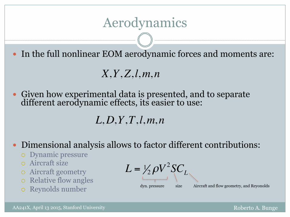
�  In the full nonlinear EOM aerodynamic forces and moments are:

�  Given how experimental data is presented, and to separate different aerodynamic effects, its easier to use:

�  Dimensional analysis allows to factor different contributions: ¡  Dynamic pressure ¡  Aircraft size ¡  Aircraft geometry ¡  Relative flow angles ¡  Reynolds number

X,Y,Z, l,m,n

L,D,Y,T, l,m,n

L = 12ρV 2SCL

dyn. pressure size Aircraft and flow geometry, and Reyonolds

Aerodynamics II


�  The dimensionless forces and moments are a function of:

i.  Aircraft geometry (fixed): AR, taper, dihedral, etc.

ii.  Control surface deflections

iii. Relative flow angles: iv.  Reynolds number:

�  Alfa and lambda: dependence is nonlinear and should be preserved if possible

�  The rest can be represented with linear terms (Stability and Control Derivatives)

�  At low AoA some stability derivatives depend on alfa, and at high angles of attack all are affected by alf

α ≈wV, β ≈

vV, λ =

VΩR

, p = pb2V, q = qc

2V, r = rb

2V

δe,δa,δr

CL,CD,CY ,CT ,Cl,C m,Cn

Re = ρcVµ

if the variation of speeds is small, it can be assumed constant and factored out

Stability and Control Derivatives


Stability Derivtaives Control Deriva1ves Nonlinear/Trim

CL

CD

CY

Cl

Cm

Cn

CT

CLq CLδe

CDq

Cmq

!α β p rq δe δa δr α λ

CT (λ)

CL (α,λ)

CD (α,λ)

Cm (α,λ)

CnβCnp

Cnr

Cmδe

CnδaCnδr

Cmα

ClβClp

CYβ

CDα

CLα

CDδe

CYr

Clr

CYδr

ClδaClδr

Cn (λ)

Cl (λ)

are small angular deflections w.r.t. a zero position, usually the trim deflection

δ

is an angle of attack perturbation around !α

α

~zero

Minor importance

Estimate via calculations

Estimate via calculations or flight testing

Estimate or trim out via flight testing

Hard to estimate

Stability and Control Derivatives II


�  Examples of force and moment expressions:

�  Example dimensionless pitching equation*:

Cl =Clpp+Clδa

δa +Clββ +Clδr

δr

CL =CL (α0,λ)+CLα!α +CLq

q+CLδe(δe −δe0 )

Cm =Cm (α0,λ)+Cmα!α +Cmq

q+Cmδe(δe −δe0 )

Lift:

Rolling moment:

Pitching moment:

I xx !q =Cm =Cm (α0,λ)+Cmα!α +Cmq

q+Cmδe(δe −δe0 )

* Neglecting gyroscopic terms

Aerodynamics IV


Bihrle, et. al. (1978) LSPAD, Selig, et. al. (1997)

Zilliac (1983)

Trim Analysis

�  Flight conditions at which if we keep controls fixed, the aircraft will remain at that same state (provided no external disturbances)

�  For each aircraft there is a mapping between trim states and trim control inputs ¡  Analogy: car going at constant speed, requires a constant throttle position

�  The mapping g() is not always one-to-one, could be many-to-many!

�  If internal dynamics are stable, then flight condition converges on trim condition

Aircraft EOM

Xtrim

δtrim

!X = 0

!X = f (Xtrim,δtrim ) = 0 Xtrim = gtrim (δtrim )


An idea: Trim + Regulator Controller

I.  Inverse trim: set control inputs that will take us to the desired state II.  Regulator: to stabilize modes and bring us back to desired trim state in

the presence of disturbances

Xdesired δtrimTrim Relations/Tables

Aircraft EOM

δ

Linear Regulator Controller

δ '+

+

+

-

X


Longitudinal Trim

�  Simple wing-tail system

L_wing

L_tail mg

h_cg h_tail

M_wing


Longitudinal Trim (II)

�  Moment balance: 0 =Mwing − hCGLwing + xtailLtail

→ 0 =1 2ρV 2 cwingSwingCmwing− hCGSwingCLwing

+ htailStailCLtail#$

%&

⇒hCGcwing

CLwing(αtrim ) =

htailStailcwingSwing

CLtail(αtrim,δetrim )−Cmwing

Elevator trim defines trim AoA, and consequently trim CL


Longitudinal Trim (III)

�  Force balance*

L

D mg

T γ

γ

V θ αmg = Lcos(γ ) ≈ L = 1

2ρV 2SCL

⇒V 2 =mg

12ρSCL (δetrim )

T = D+ Lsin(γ ) ≈ D+ Lγ

⇒ γ =T(δttrim )mg

−1

(LD)(δetrim )

Trim Elevator defines trim Velocity!

Elevator & Thrust both define Gamma! *Assuming small Gamma


Longitudinal Trim (IV)

�  How do we get an aircraft to climb? (Gamma > 0)

�  Two ways: 1.  Elevator up

÷  Elevator up increases AoA, which increases CL ÷  Increased CL, accelerates aircraft up ÷  Up acceleration, increases Gamma ÷  Increased Gamma rotates Lift backwards, slowing down the aircraft

2.  Increase Thrust ÷  Increased thrust increases velocity, which increases overall Lift ÷  Increased Lift, accelerates aircraft up ÷  Up acceleration, increases Gamma ÷  Increased Gamma rotates Lift backwards, slowing down the aircraft to original speed (set by

Elevator, remember!)

�  Elevator has its limitations ¡  When L/D max is reached, we start going down ¡  When CL max is reached, we go down even faster!


Experimental Trim Relations

�  Theoretical relations hold to some degree experimentally �  In reality:

¡  Propeller downwash on horizontal tail has a significant distorting effect ¡  Reynolds variations with speed, distort aerodynamics

�  One can build trim tables experimentally ¡  Trim flight at different throttle and elevator positions ¡  Measure:

÷  Average airspeed ÷  Average flight path angle Gamma

¡  Phugoid damper would be very helpful

�  One could almost fly open loop with trim tables!


Turning Maneuver

�  Centripetal force balance:

�  Minimum turn radius:

�  Depends on:

L

mg

φ

mV 2

R = mV !εLsin(φ) = mV

2

R

⇒ R = mV 2

12ρV 2SCL sin(φ)

=mS

112ρCL sin(φ)


Rmin =mS

112ρCLmax

sin(φmax )

φmax,mS&CLmax

0"

10"

20"

30"

40"

50"

60"

0" 10" 20" 30" 40" 50" 60" 70" 80"

turn%ra

dius%(m

)%

roll%angle%(deg)%

Minimum%Turn%Radius%(wing%loading%=%35%g/dm^2)%

CL"="0.6"

CL"="0.8"

CL"="1.0"

Turning Maneuver II


�  What are the constraints on maximum turn? 1.  Elevator deflection to achieve high CL in a turn 2.  Do we care about loosing altitude? 3.  Maximum speed and thrust 4.  Controls: maneuver can be short lived, so high bandwidth is require for tracking tracking

1.  Roll tracking, etc. 2.  Sensor bandwidth

5.  Maximum G-loading 6.  Maximum CL and stall 7.  Aerolasticity of controls at high loading

�  Elevator to achieve CL: ¡  The pitching moment balance equation in dimensionless form:

¡  Assume that before the turn we have trimmed the aircraft in level flight at the desired alfa (CL):

I xx !q =Cm (α,λ0 )+Cmqq+Cmδe

(δe −δe0 )

⇒Cmδeδe0 =Cm (α,λ0 )

Turning Maneuver III


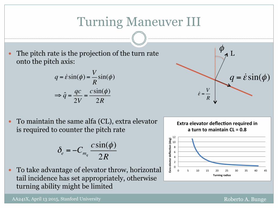
�  The pitch rate is the projection of the turn rate onto the pitch axis:

�  To maintain the same alfa (CL), extra elevator

is required to counter the pitch rate

�  To take advantage of elevator throw, horizontal

tail incidence has set appropriately, otherwise turning ability might be limited

δe = −Cmq

csin(φ)2R

q = !ε sin(φ) = VRsin(φ)

⇒ q = qc2V

=csin(φ)2R

L φ

q = !ε sin(φ)!ε = V

R

0"

2"

4"

6"

8"

10"

12"

0" 5" 10" 15" 20" 25" 30" 35" 40" 45"Exra%elevtor%defl

ec.o

n%(deg)%

Turning%radius%

Extra%elevator%deflec.on%required%in%a%turn%to%maintain%CL%=%0.8%

Linearized Dynamics Analysis

�  Many flight dynamic effects can be analyzed & explained with Linearized Dynamics

�  Most of the times we linearize dynamics around Trim conditions

�  Useful to synthesize linear regulator controllers ¡  Provide stability in the face of uncertainty in different dynamic parameters ¡  They help in rejecting disturbances ¡  They can also help in going from one trim state to the another, provided they are not “too far away”

Aircraft EOM (near Trim)

Xtrim + X'

δtrim +δ'

!X = ∂f∂X

X ' +∂f∂δδ '


Linearized Dynamics

�  Limited to a small region (what does “small” mean?) ¡  Especially due to trigonometric projections and nonlinear alfa

dependences

�  In practice, nonlinear dynamics bear great resemblance ¡  We can gain a lot of insight by studying dynamics in the vicinity a flight

condition �  We can separate into longitudinal and lateral dynamics

(If aircraft and flight condition are symmetric)

�  Linearized models also provide some information about trim relations


Longitudinal Static Stability

�  Static stability ¡  Does pitching moment increase when AoA increases? ¡  If so, then divergent pitch motion (a.k.a statically unstable)

�  CG needs to be ahead of quarter chord!

�  As CG goes forward, static margin increases, but… more elevator deflection is required for trim and trim drag increases

Lw (α)

Lw (α +Δα)

CG ahead CG behind

Restoring moment

Divergent moment


Longitudinal Dynamics

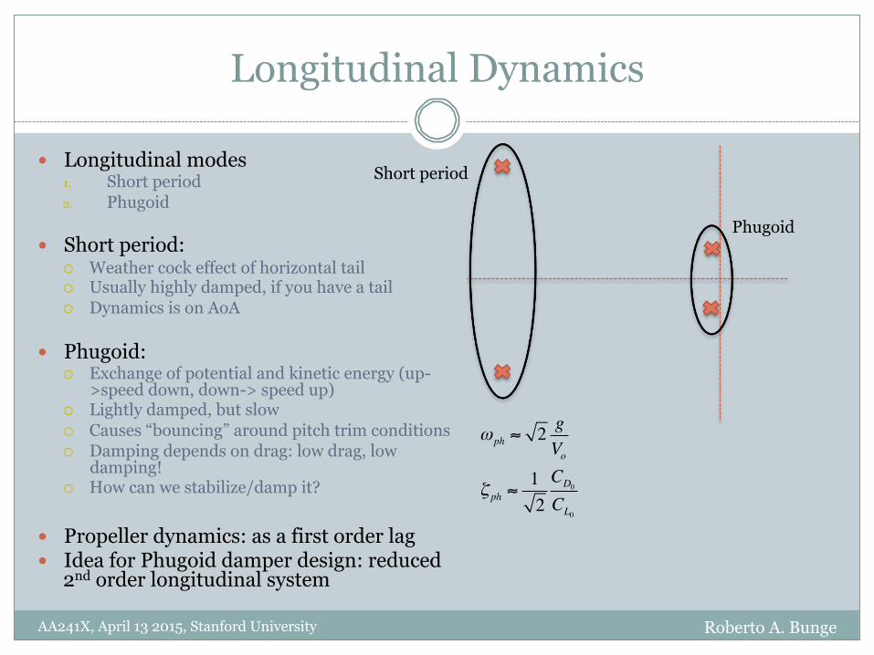
�  Longitudinal modes 1.  Short period 2.  Phugoid

�  Short period: ¡  Weather cock effect of horizontal tail ¡  Usually highly damped, if you have a tail ¡  Dynamics is on AoA

�  Phugoid: ¡  Exchange of potential and kinetic energy (up-

>speed down, down-> speed up) ¡  Lightly damped, but slow ¡  Causes “bouncing” around pitch trim conditions ¡  Damping depends on drag: low drag, low

damping! ¡  How can we stabilize/damp it?

�  Propeller dynamics: as a first order lag �  Idea for Phugoid damper design: reduced

2nd order longitudinal system

Short period

Phugoid


ω ph ≈ 2 gVo

ζ ph ≈12CD0

CL0

Lateral Dynamics

�  Lateral-Directional modes: 1.  Roll subsidence 2.  Dutch roll 3.  Spiral

�  Roll subsidence: ¡  Naturally highly damped ¡  “Rolling in honey” effect

�  Dutch roll: ¡  Oscillatory motion ¡  Usually stable, and sometimes lightly damped ¡  Exchange between yaw rate, sideslip and roll rate

�  Spiral: ¡  Usually unstable, but slow enough to be easily stabilized

�  Dutch Roll and Spiral stability are competing factors ¡  Dihedral and vertical tail volume dominate these

�  Note: see “Flight Vehicle Aerodynamics”, Ch. 9 for more details

Dutch roll

Spiral Roll subsidence


σ roll ≈12ρVoSb

2

IxxClp

σ spiral ≈12ρVoSb

2

Izz(Cnr

−Cnβ

Clr

Clβ

)

Vortex Lattice Codes

�  Good at predicting inviscid part of attached flow around moderate aspect ratio lifting surfaces

�  Represents potential flow around a wing by a lattice of horseshoe vortices


VLM Codes (II)

�  Viscous drag on a wing, can be added for with “strip theory” ¡  Calculate local Cl with VLM ¡  Calculate 2D Cd(Cl) either from a polar plot of airfoil ¡  Add drag force in the direction of the local velocity

�  Usually not included: ¡  Fuselage

÷  can be roughly accounted by adding a “+” lifting surface ¡  Propeller downwash

�  VLMs can roughly predict: ¡  Aerodynamic performance (L/D vs CL) ¡  Stall speed (CLmax) ¡  Trim relations ¡  Stability Derivatives

÷  Linear control system design ÷  Nonlinear Flight simulation (non-dimensional aerodynamics is linear, but dimensional

aerodynamics are nonlinear and EOMs are nonlinear)


VLM Codes (III)

�  AVL: ¡  Reliable output ¡  Viscous strip theory ¡  No GUI & cumbersome to define geometry

�  XFLR: ¡  Reliable output ¡  Viscous strip theory ¡  GUI to define geometry ¡  Good analysis and visualization tools

�  Tornado ¡  I’ve had some discrepancies when validating against AVL ¡  Written in Matlab

�  QuadAir ¡  Good match with AVL ¡  Written in Matlab ¡  Easy to define geometries ¡  Viscous strip theory soon ¡  Originally intended for flight simulation, not aircraft design

÷  Very little native visualization and performance analysis tools


Recommended Readings


1.  Fundamentals of Flight, Shevell ¡  Big picture of Aerodynamics, Flight Dynamics and Aircraft Design

2.  Dynamics of Flight, Etkin ¡  Very good development of trim and linearized flight dynamics and aerodynamics. Some

ideas for control

3.  Flight Vehicle Aerodynamics, Drela ¡  Great mix between real world and mathematical aerodynamics and flight dynamics. No

controls. Ch. 9 very clear and useful development of linearized models

4.  Automatic Control of Aircraft and Missiles, Blakelock ¡  In depth description of flight EOMs and many ideas for linear regulators

5.  Low-speed Aerodynamics, Plotkin & Katz ¡  Great book on panel methods (only if you want to write your own panel code)

Documents

Roberto!A.Bunge AA241X April132015 …adl.stanford.edu/groups/aa241x/wiki/e054d/attachments...Longitudinal & Lateral Decoupling AA241X, April 13 2015, Stanford University Roberto A