Roberto Roson

PAMS.py:

a GAMS-like Modeling System based on Python

and SAGE ISSN: 1827-3580 No. 23/WP/2016

W o r k i n g P a p e r s D e p a r t m e n t o f E c o n o m i c s

C a ’ F o s c a r i U n i v e r s i t y o f V e n i c e N o . 2 3 / W P / 2 0 1 6

ISSN 1827-3580

The Working Paper Series is available only on line

(http://www.unive.it/nqcontent.cfm?a_id=86302) For editorial correspondence, please contact:

wp.dse@unive.it

Department of Economics Ca’ Foscari University of Venice Cannaregio 873, Fondamenta San Giobbe 30121 Venice Italy Fax: ++39 041 2349210

PAMS.py:

a GAMS-like Modeling System based on Python and SAGE

Roberto Roson Ca’ Fo s ca r i Un i v e r s i t y o f Ven i c e , Depa r tmen t o f E conom i c s

Abstract This paper presents an external module for the Python programming language and for the SAGE open source mathematical software, which allows the realization of models based on constrained optimization or non-linear systems. The module, which is freely available for download, allows describing the structure of a model using a syntax similar to that of popular modeling systems like GAMS, AIMMS or GEMPACK; in particular by allowing the automatic replication of equations, variable and parameter definitions on the basis of some specified sets. Keywords GAMS, Python, SAGE, AIMMS, CGE, optimization software, applied economic modeling JEL Codes C63, C65, C68, C8

Address for correspondence: Roberto Roson

Department of Economics Ca’ Foscari University of Venice

Cannaregio 873, Fondamenta S.Giobbe 30121 Venezia - Italy

Fax: (++39) 041 2349176 E - m a i l : roson@unive.it

This Working Paper is published under the auspices of the Department of Economics of the Ca’ Foscari University of Venice. Opinions expressed herein are those of the authors and not those of the Department. The Working Paper series is designed to divulge preliminary or incomplete work, circulated to favour discussion and comments. Citation of this paper should consider its provisional character.

PAMS.py:

a GAMS-like Modeling System

based on Python and SAGE

Roberto Roson1

September 2016

ABSTRACT

This paper presents an external module for the Python programming language and for the

SAGE open source mathematical software, which allows the realization of models based on constrained optimization or non-linear systems. The module, which is freely available for

download, allows describing the structure of a model using a syntax similar to that of popular modeling systems like GAMS, AIMMS or GEMPACK; in particular by allowing the automaticreplication of equations, variable and parameter definitions on the basis of some specified sets.

KEYWORDS: GAMS, Python, SAGE, AIMMS, CGE, optimization software, applied economic

modeling.

JEL Codes: C63, C65, C68, C88.

1 Dipartimento di Scienze Economiche, Ca'Foscari University, Venice and IEFE, Bocconi University, Milan. E-Mail: roson@unive.it .

1

1. Introduction

Many applied models, especially in economics, are based on non-linear constrained optimization and

system solving. Years ago, the standard way to realize simulations for this kind of models involved writing your own code, using a programming language like FORTRAN, possibly making calls to external math library subroutines. Subsequently, the introduction of packages like Matlab, GAUSS, Octave, R and many others have made this process somewhat simpler, because vectors and matrices can be treated as single variables, and complex numerical tasks can be performed with a single

instruction. Furthermore, math software like Matlab gives access to a wide array of libraries and specifically tailored algorithms (including parallel computation tools) for many scientific applications.However, one fundamental problem remains: the model code still looks much different from the more familiar mathematical notation one normally uses in a research work. Therefore, checking and modifying the model code written by another researcher may become a rather daunting (and error-

prone) task.To address this issue, GAMS (General Algebraic Modeling System) was developed by Alexander Meeraus and many of his collaborators at the World Bank in Washington D.C., since the late '70s (Meeraus, 1983). The main purpose of GAMS was (and still is) “providing a high-level language for

the compact representation of large and complex models” and “permitting model descriptions that are independent of solution algorithms”.

Two fundamental principles are adopted to this end. First, the model description is kept separated from the algorithm used to solve the model. The model description in GAMS is an ordinary text file (usually with the “.gms” extension), which can be edited with a normal text editor. Modern versions of GAMS

include a Graphical User Interface (GUI), helping the modeler to define the structure of the model through an interactive process, but the final result is still a plain gms text file. A fellow researcher, with

a minimum basic knowledge of the GAMS syntax, can then easily interpret what the model is about: what equations are in it, what is maximized or minimized, etc. GAMS itself does not solve the model. Rather, it translates the model description into a computer code digestible to some external solver, call

that solver, and processes the solver’s output to give an easily understandable text file of results (plus graphical output in the recent versions).

The model description is based on the principle of indexing of parameters, variables and equations, which is discussed in some more detail in the next section. This means, for instance, that not all equations need to be written down in the input file, but only “representative” equations, valid for a set

of variables.

This paper presents an external module for the Python programming language and for the SAGE open source mathematical software, based on the key principles underlying GAMS and other similar packages. The purpose is providing a tool that takes the best of both worlds: the simplicity and clarity of GAMS-like systems combined with the flexibility and power of Python and SAGE. PAMS.py, whichis a plain text file, can be examined and downloaded freely at: http://venus.unive.it/roson/Soft.htm,

where a compact reference manual can also be retrieved.The paper is structured as follows. In the next section, some key characteristics of GAMS and other popular Modeling Systems are reviewed in some detail. Section 3 introduces the Python programming language and the closely related SAGE system for symbolic and numerical computation. Section 4 illustrates the basics of the PAMS.py syntax, and in Section 5 a practical example is provided. A

discussion follows in Section 6 and a final section concludes.

2

2. Indexing in GAMS and other popular Modeling Systems

A model is described in GAMS through an ordinary text file, which has a structure and a syntax that

closely resembles the standard mathematical notation. One central concept in the GAMS language is the automatic indexing of variables, parameters and equations (Brooke et al., 1998). For example, if there are many markets indexed by i, then P(i) could be the equilibrium price for them, determined by an equation EQUIL(i), matching supply and demand (possibly linear functions of some parameters a, b, c and d). In GAMS notation, all this is expressed as:

Set i markets / new-york, chicago, topeka /;Parameters a(i), b(i), c(i), d(i);Variable P(i) equilibrium price in market i;Positive Variable P;Equation EQUIL(i) equilibrium condition in market i;EQUIL(i).. a(i)+b(i)*P(i)=E=c(i)-d(i)*P(i);

When the GAMS interpreter reads the code above, it generates three sets of parameters, three price variables and three equations, one for each of the markets. To add more markets, one has only to add

more elements in the set i. A model in GAMS is basically a group of equations which, depending on thecontext, are interpreted as a system, as constraints in an optimization problem, as complementarity

conditions, etc.A similar indexing mechanism is used by AIMMS (Bisschop, 2006), a mathematical modeling tool introduced in 1993 and very similar to GAMS in many respects, including its role as interface towards

external solvers. Although models are typically formulated in AIMMS in an interactive way, through a Graphical User Interface (GUI), the model description can be found inside an ordinary (and editable)

text file, much like GAMS (Bisschop and Roelofs, 2004).For instance, the definition of a price variable P over a set of elements i is stated in an AIMMS model code as:

Variable P { IndexDomain: i; Range: nonnegative; }

And an equation (automatically replicated for all elements in the sets i x h) is expressed as:

Constraint CONSDEM { IndexDomain: (i,h); Definition: P(i)*QQ(i,h) = IN(h)*IO(i,h); }

Another popular modeling system, which also uses automatic indexing based on sets, is GEMPACK

(Codsi and Pearson, 1998). GEMPACK is almost only used for building and running CGE models (Horridge and Pearson, 2011) but, unlike GAMS and AIMMS, it does not interface with external solvers and it is only intended to handle (large) non-linear systems (Pearson, 1988, Harrison and Pearson, 1996).

3

A GEMPACK model is described in a text file using a language called TABLO. Here is an example of a price variable definition in TABLO, valid for all elements in the set TRAD_COMM (previously defined) and all elements in the set REG:

Variable (all,i,TRAD_COMM)(all,s,REG) ppd(i,s) # price of domestic i to private households in s #;

Whereas an equation is formulated in a similar way, for example as:

Equation PHHDPRICE# eq'n links domestic market and private consumption prices (HT 18) #(all,i,TRAD_COMM)(all,r,REG) ppd(i,r) = atpd(i,r) + pm(i,r);

3. Python and SAGE

Over the last decade, Python has become one of the core languages of scientific computing, and it is increasingly being used to implement numerical models in economics and statistics (see, e.g.,

http://lectures.quantecon.org/py/index.html; Sargent and Stachurski, 2016). Python is free and open source, and it is supported by a vast collection of standard and external software libraries, including:

NumPy and SciPy (array processing capabilities, numerical calculus), Matplotlib (graphics), SymPy (symbolic algebra), Pandas (statistics), NetworkX (graphs).A Python interpreter is included in most Linux distributions and MacOS. For other versions, libraries,

documentation, complementary software, etc., see http://www.python.org.SAGE is a free open source alternative to commercial programs like Magma, Maple, Mathematica, and

Matlab (Stein, 2012). It combines about 100 open-source packages with a large amount of new code, and provides both a sophisticated multiuser web-based graphical user interface and a powerful command line interface. SAGE can be obtained at http://www.sagemath.org, where documentation and

other material can be found as well.SAGE is based on Python (indeed, it can be seen as a bundled Python distribution with pre-linked and

compiled external libraries). It includes a Python interpreter and, for this reason, one can use almost anything ever written in Python directly inside SAGE.

4. How to use the PAMS.py module

Python allows loading external modules (thus, SAGE as well), that are pieces of codes which, once loaded, can be interpreted and therefore can make some extra functionalities available. The Python

language is object-oriented, meaning that “classes” of objects can be defined, each one with specific properties and actions that can be undertaken with all objects belonging to the class. PAMS.py is an external module for Python and SAGE, defining classes for parameters, variables, equations and models, in a way similar to GAMS. First, the module must be loaded and made available to the Python interpreter, which can be done by

issuing the command:

load('[path]/PAMS.py')

where [path] is a path for the directory containing the file PAMS.py. The module, which is a standard

4

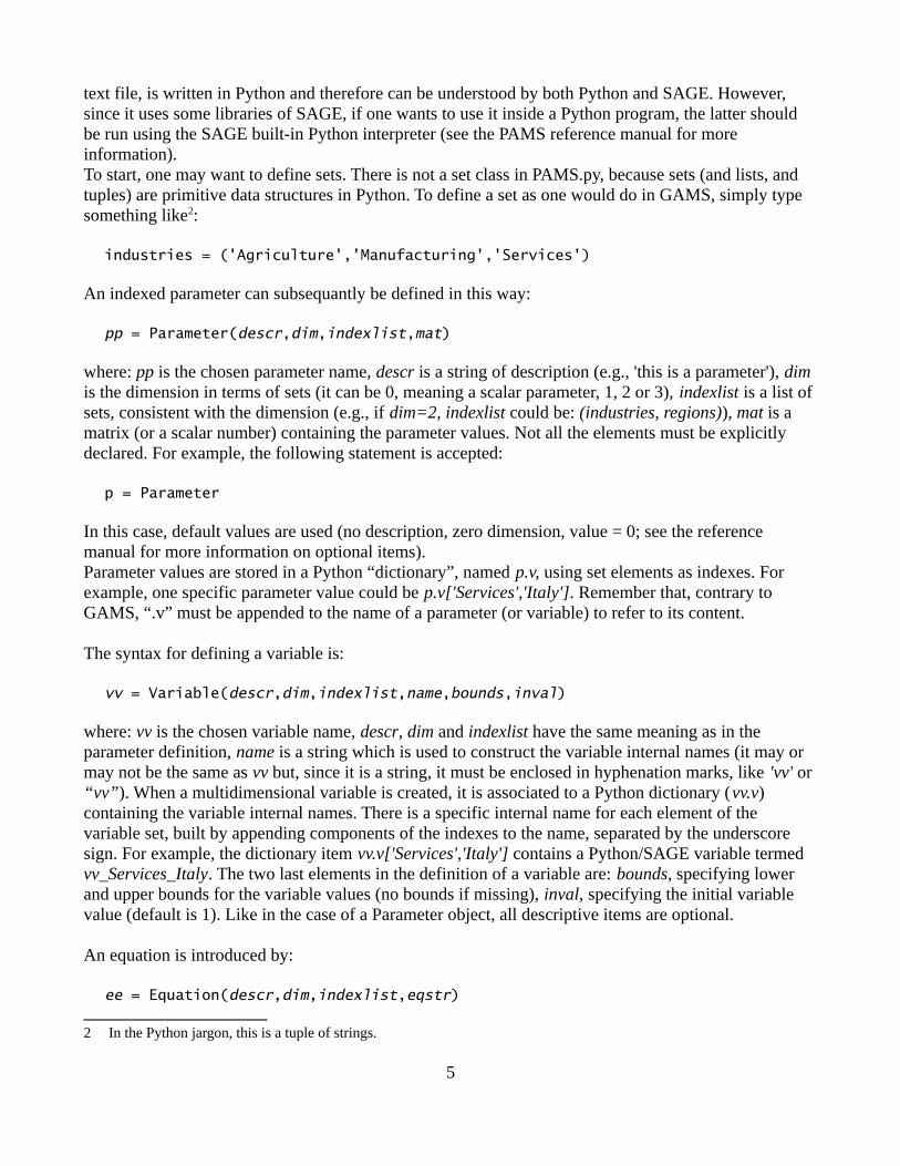
text file, is written in Python and therefore can be understood by both Python and SAGE. However, since it uses some libraries of SAGE, if one wants to use it inside a Python program, the latter should be run using the SAGE built-in Python interpreter (see the PAMS reference manual for more information).To start, one may want to define sets. There is not a set class in PAMS.py, because sets (and lists, and

tuples) are primitive data structures in Python. To define a set as one would do in GAMS, simply type something like2:

industries = ('Agriculture','Manufacturing','Services')

An indexed parameter can subsequantly be defined in this way:

pp = Parameter(descr,dim,indexlist,mat)

where: pp is the chosen parameter name, descr is a string of description (e.g., 'this is a parameter'), dim is the dimension in terms of sets (it can be 0, meaning a scalar parameter, 1, 2 or 3), indexlist is a list of

sets, consistent with the dimension (e.g., if dim=2, indexlist could be: (industries, regions)), mat is a matrix (or a scalar number) containing the parameter values. Not all the elements must be explicitly

declared. For example, the following statement is accepted:

p = Parameter

In this case, default values are used (no description, zero dimension, value = 0; see the reference

manual for more information on optional items).Parameter values are stored in a Python “dictionary”, named p.v, using set elements as indexes. For example, one specific parameter value could be p.v['Services','Italy']. Remember that, contrary to

GAMS, “.v” must be appended to the name of a parameter (or variable) to refer to its content.

The syntax for defining a variable is:

vv = Variable(descr,dim,indexlist,name,bounds,inval)

where: vv is the chosen variable name, descr, dim and indexlist have the same meaning as in the parameter definition, name is a string which is used to construct the variable internal names (it may or

may not be the same as vv but, since it is a string, it must be enclosed in hyphenation marks, like 'vv' or “vv”). When a multidimensional variable is created, it is associated to a Python dictionary (vv.v) containing the variable internal names. There is a specific internal name for each element of the variable set, built by appending components of the indexes to the name, separated by the underscore sign. For example, the dictionary item vv.v['Services','Italy'] contains a Python/SAGE variable termed

vv_Services_Italy. The two last elements in the definition of a variable are: bounds, specifying lower and upper bounds for the variable values (no bounds if missing), inval, specifying the initial variable value (default is 1). Like in the case of a Parameter object, all descriptive items are optional.

An equation is introduced by:

ee = Equation(descr,dim,indexlist,eqstr)

2 In the Python jargon, this is a tuple of strings.

5

where: ee is the equation name, descr, dim and indexlist have the usual meaning, eqstr is a string

(thereby enclosed in hyphenation marks) describing the equation. The rules for writing the equation

are:

• The Python/SAGE syntax for mathematical expressions is followed. All SAGE pre-defined

functions (e.g., sqrt, sin, log, sum, prod) can be used, as well as previously defined user

functions.

• The equality sign is '==' (“>”, “>=”, “<=”,”<” can also be used to define constraints for

numerical optimization).

• If the right hand side is MIN or MAX, the left hand side is interpreted as a function to be

minimized or maximized, respectively. There can be multiple MIN or MAX equations, as in this

case they are algebraically added to form the objective function. The other equations in the

model are interpreted as constraints.

• All parameters and all variables must be referred to by their own names, followed by “.v”. Set

indexes for parameters and variables are enclosed in square parentheses.

• A running index, that is an index which is used to create copies of the same equation over

elements of a set, must be indicated with the mark §i for the first set in indexlist, §j for the

second one, §k for the third one.

• It is possible to use Python iterators in expressions. This is especially useful to make

summations (or products). For example, sum(QQ.v[j,§i]*P.v[j] for j in industries) is

a legitimate expression, involving one running index §i and one summation index j.

A model is simply declared by:

mm = Model(eqlist,varlist)

where: mm is the model name, eqlist and varlist are lists of equations and variables in the model. The

two lists can be specified directly inside the statement or as list objects defined beforehand. No specific

ordering of equations or variables is required.

Once a model has been declared, several actions or “methods” can be undertaken on it. To invoke a

method (in Python), it is possible to write the model name, followed by a dot, then the method name,

then a couple of parentheses, where the values for parameters are given. If there are no parameters or if

one wants to accept the default parameter values, just type “()”.

Methods for Model objects are described in the reference manual. Among them:

mm.solve()

Tries to solve the mm model symbolically, possibly identifying multiple solutions. This may work only

with simple models, otherwise the numerical method nsolve should be used. If it works, the method

prints the result and returns a Python dictionary mm.solution, containing the outcome, which could

then be further elaborated.

mm.nsolve()

Numerical system solving. Initial points are specified by inval in the variable definitions. method (the

only optional parameter) indicates the solution algorithm used by the invoked scipy.optimize routine

root; hybr is the default, alternatives are: lm, broyden1, broyden2, anderson, linearmixing,

6

diagbroyden, excitingmixing, krylov. See the SciPy documentation for the proper use of these alternative algorithms. The solution is printed (shown on screen) when the method is invoked, together with information about the convergence process. In case of successful convergence, likewise solve, it returns the Python dictionary mm.solution.

mm.nopt()

Numerically optimize the model, using the minimize function in the scipy.optimize library. The list of equations in the model must contain at least one equation with MIN or MAX on the left hand side, to define the objective function. Furthermore, it can contain any number of equality and inequality

expressions, which are then interpreted as constraints, possibly in addition to lower and upper bounds for the variables. The solution shown on screen, together with information about the convergence process. Again, in case of success, it returns mm.solution.

5. Example: Implementation of a very simple CGE model

To illustrate the use of the PAMS.py module, we show here how a very simplified Computable General

Equilibrium model can be implemented with PAMS.py and how it is possible to carry out some simulation exercises.

A commented log (pdf file) of the corresponding SAGE session can be found at:http://venus.unive.it/roson/Soft.htmIn the same directory, other useful documents can be retrieved, namely:

• the PAMS.py module itself, which is a text file;

• the PAMS.sage module for direct use within SAGE;

• the PAMS.py/PAMS.sage reference pdf manual;

• the equivalent formulation of the simple CGE model in GAMS;

• the equivalent formulation of the simple CGE model in AIMMS;

• the GAMS linear programming transportation problem (from the GAMS introductory tutorial);

• the same problem in PAMS.py (pdf log of interactive session);

• the same problem in AIMMS;

Let us assume that a Social Accounting Matrix (SAM) is available, describing income flows in a closed

economy, composed of three productive sectors, one final consumer and one primary resource. This SAM, showed in Table 1, can be used to calibrate the structural parameters of a CGE model. Negative numbers indicate (net) income generation, positive numbers expenses. Because of accounting identities, all sums by row or column are zero.

Table 1 – A fictitious SAM

Agriculture Manufacturing Services Household

Agriculture -10 5 2 3

Manufacturing 5 -20 8 7

Services 2 10 -20 18

Labor 3 5 20 -28

7

This SAM can be introduced in Python as a matrix, with this command:

sam=matrix([[-10.,5.,2.,3.],[5.,-20.,8.,7.],[2.,10.,-30.,18.],

[3.,5.,20.,-28.]])

Sets are directly defined as Python tuples. Let us define three industries ('Ag','Ma','Se'), one household

or final consumption agent ('C'), one primary resource ('L'):

ind=('Ag','Ma','Se');hou=('C');res=('L')

Row headers are industries and primary resources, column headers are industries and final demand

agents:

rowh=tuple(list(ind)+list(res)); colh=tuple(list(ind)+list(hou));

From the SAM above, let us extract an input-output matrix, where it is assumed that all industries do

not buy intermediate factors from themselves (therefore, negative numbers along the main diagonal

express, with reversed sign, the industrial output). Also, let us derive a reduced IO matrix, restricted to

intermediate factors. This will turn out useful later, because we shall assume that intermediate factors

are not substitutable among themselves. Some Python instructions to achieve this are:

IOmat=matrix(RR,len(rowh),len(colh))

for j in range(len(colh)):

for i in range(len(rowh)):

if i==j:

IOmat[i,j]=0

else:

IOmat[i,j]=sam[i,j]/(-sam[j,j])

IORmat=matrix(RR,len(ind),len(ind))

for j in range(len(ind)):

for i in range(len(ind)):

IORmat[i,j]=IOmat[i,j]/sum(IOmat[k,j] for k in

range(len(ind)))

Now we can start defining parameters. If the PAMS.py has been previously loaded, we can introduce

the IO (multidimensional) parameter, with values (IO.v) obtained from the IOmat matrix. Its

dimensions are rowh x colh. Elements in these two sets will be later used as indexes.

IO=Parameter('Input-output coefficients derived from the SAM',2,

(rowh,colh),IOmat)

Analogously, for intermediate factors:

IOR=Parameter('Input-output coefficients for the intermediate

bundle',2,(ind,ind),IORmat)

Physical endowment of primary resources by the representative consumer is:

8

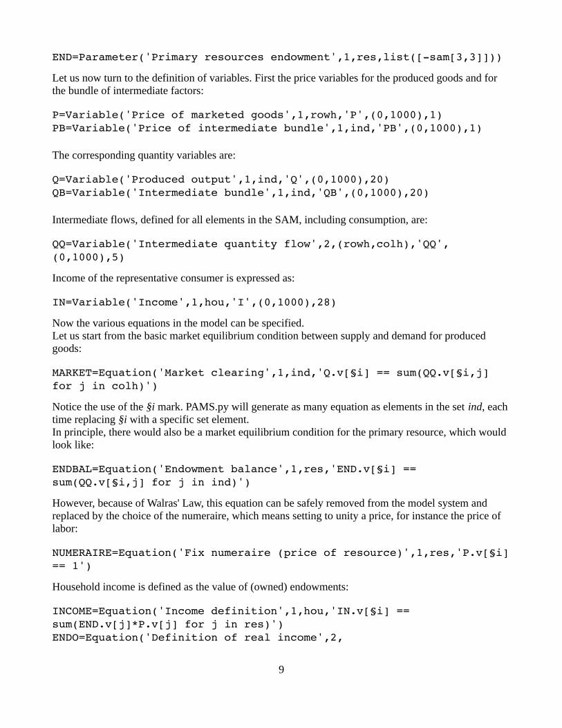
END=Parameter('Primary resources endowment',1,res,list([-sam[3,3]]))

Let us now turn to the definition of variables. First the price variables for the produced goods and for

the bundle of intermediate factors:

P=Variable('Price of marketed goods',1,rowh,'P',(0,1000),1)

PB=Variable('Price of intermediate bundle',1,ind,'PB',(0,1000),1)

The corresponding quantity variables are:

Q=Variable('Produced output',1,ind,'Q',(0,1000),20)

QB=Variable('Intermediate bundle',1,ind,'QB',(0,1000),20)

Intermediate flows, defined for all elements in the SAM, including consumption, are:

QQ=Variable('Intermediate quantity flow',2,(rowh,colh),'QQ',

(0,1000),5)

Income of the representative consumer is expressed as:

IN=Variable('Income',1,hou,'I',(0,1000),28)

Now the various equations in the model can be specified.

Let us start from the basic market equilibrium condition between supply and demand for produced

goods:

MARKET=Equation('Market clearing',1,ind,'Q.v[§i] == sum(QQ.v[§i,j]

for j in colh)')

Notice the use of the §i mark. PAMS.py will generate as many equation as elements in the set ind, each

time replacing §i with a specific set element.

In principle, there would also be a market equilibrium condition for the primary resource, which would

look like:

ENDBAL=Equation('Endowment balance',1,res,'END.v[§i] ==

sum(QQ.v[§i,j] for j in ind)')

However, because of Walras' Law, this equation can be safely removed from the model system and

replaced by the choice of the numeraire, which means setting to unity a price, for instance the price of

labor:

NUMERAIRE=Equation('Fix numeraire (price of resource)',1,res,'P.v[§i]

== 1')

Household income is defined as the value of (owned) endowments:

INCOME=Equation('Income definition',1,hou,'IN.v[§i] ==

sum(END.v[j]*P.v[j] for j in res)')

ENDO=Equation('Definition of real income',2,

9

(res,hou),'QQ.v[§i,§j]==IN.v[§j]/P.v[§i]')

We assume that the representative consumer has a Cobb-Douglas utility function, implying that the cost

shares are constant:. This condition indirectly defines final consumption by the household:

CONSDEM=Equation('Consumption demand',2,

(ind,hou),'P.v[§i]*QQ.v[§i,§j] == IN.v[§j]*IO.v[§i,§j]') # Cobb-

Douglas

The production functions are of nested Cobb-Douglas/Leontief type, with unitary elasticity of

substitution between labor and the bundle of intermediate inputs, zero elasticity among intermediates.

This brings about the following demand functions:

BUNDLE=Equation('Int. demand bundle',1,ind,'P.v[§i]*Q.v[§i]*(1-

IO.v["L",§i]) == PB.v[§i]*QB.v[§i]') # Cobb-Douglas

INTERM=Equation('Intermediate demand',2,(ind,ind),'QQ.v[§i,§j] ==

QB.v[§j]*IOR.v[§i,§j]') # Leontief

RESDEM=Equation('Resources demand',2,(res,ind),'P.v[§i]*QQ.v[§i,§j]

== P.v[§j]*Q.v[§j]*IO.v[§i,§j]') # Cobb-Douglas

The zero profit conditions ensures that the unit price of all goods equates the minimum production cost

(a CD cost function):

ZEROP=Equation('Zero profit, price equals cost',1,ind,'P.v[§i] ==

(P.v["L"]**IO.v["L",§i])*(PB.v[§i]**(1-IO.v["L",§i]))')

The model is now ready:

mod_eq= [MARKET,INCOME,ENDO,SETPB,ZEROP,BUNDLE,INTERM,RESDEM,CONSDEM,

NUMERAIRE]

mod_var=[P,PB,Q,QB,QQ,IN]

SIMPLECGE=Model(mod_eq,mod_var)

Perhaps we may want to look at how the model system looks like after our commands have been

processed by PAMS.py…

SIMPLECGE.equations()

… or to check whether the number of equations is the same as the number of variables (30 in our case):

print len(SIMPLECGE.initialvalues)

print len(SIMPLECGE.elist)

Everything is correct, so we can go on with the usual “calibration round”, where we expect that all

prices will be equal to one in equilibrium:

SIMPLECGE.nsolve()

The nsolve command produces a lengthy output, which is not fully reported here (but can be seen in the

downloadable log file), including a list of endogenous variable values, for instance:

10

P_Ma = 1.0

P_Se = 1.0

P_Ag = 1.0

…Q_Ma = 20.0

Q_Se = 30.0

Q_Ag = 10.0

…

Now more meaningful simulations can be realized, by changing the value of some exogenous parameters. For instance, one simple experiment is varying the value of the numeraire. Since a Walrasian general equilibrium can only determine relative prices, all endogenous prices will vary to the

same direction:

NUMERAIRE=Equation('Fix numeraire (price of resource)',1,res,'P.v[§i]

== 2')

mod_eq= [MARKET,INCOME,ENDO,SETPB,ZEROP,BUNDLE,INTERM,RESDEM,CONSDEM,

NUMERAIRE]

SIMPLECGE=Model(mod_eq,mod_var)

SIMPLECGE.nsolve()

Of course, this produces something like:

P_Ma = 2.0

P_Se = 2.0

P_Ag = 2.0

…Q_Ma = 20.0

Q_Se = 30.0

Q_Ag = 10.0

…

6. Discussion: When and where could PAMS.py be advantageously used?

PAMS.py is by no means a serious alternative to packages like GAMS, AIMMS or GEMPACK, as theyoffer many more functionalities, data exchange with spreadsheets, graphical user interfaces, etc.. On the other hand, PAMS.py is totally free (likewise SAGE and Python) and the code can be inspected and

possibly improved by anyone interested and capable to do it. In fact, I am not a professional programmer and I am sure that the module can be made better in many possible ways.The main advantage of PAMS.py is given by the fact that it lives inside a SAGE/Python environment, which allows to take full advantage of the power of both languages, as well as of the availability of a huge number of libraries and complementary software, for virtually any scientific application. Indeed,

PAMS.py requires the previous installation of the SAGE mathematical software (which embeds a Python interpreter), and this is currently available for the Mac and Linux operating systems, but can also be run remotely with any browser, through an interactive session at http://www.sagemath.org.

11

Therefore, if you know quite well GAMS, AIMMS or GEMPACK and you are happy with these

packages, probably you would not need PAMS.py. However, if you have some previous knowledge of

Python, or SAGE, or if you want to attain it in the near future (which I would recommend to any

researcher), then you may like the possibility of integrating a GAMS-like model structure into a Python

or SAGE code.

7. Conclusion

This paper has presented an external module for programs written with the Python language and for the

SAGE mathematical software. This module allows the definition and solution of non-linear systems

and optimization problems, described in a way very similar to GAMS and programs alike.

The key common characteristic of PAMS.py and GAMS is the automatic indexing of parameters,

equations and variables. Since many elements of this kind can be defined with only one instruction (as

one would normally do, for instance when the model is illustrated in a scientific paper), understanding

how the model works directly by reading the program code is normally quite straightforward. The latter

feature turns out to be particularly critical when the model code needs to be understood and

manipulated by others, which may occur either in a team work or when replication and validation of

some results is called for.

References

Bisschop, J. (2006), AIMMS optimization modeling. Lulu.com.

Bisschop, J., and Roelofs, M. (2004), “The modeling language AIMMS”, in: Modeling Languages in Mathematical Optimization (pp. 71-104), Springer US.

Brooke, A., Kendrick, D., Meeraus, A., Raman, R., and America, U. (1998), The general algebraic

modeling system, GAMS Development Corporation.

Codsi, G. and Pearson, K.R. (1998) "GEMPACK: General-purpose software for applied general

equilibrium and other economic modellers.", Computer Science in Economics and Management, vol.1(3), pp.189-207.

Harrison, W. J., and Pearson, K. R. (1996), “Computing solutions for large general equilibrium models

using GEMPACK”, Computational Economics, vol.9(2), pp.83-127.

Horridge, M. and Pearson, K.R. (2011), Solution Software for CGE Modeling, General Paper No. G-

214, Centre of Policy Studies, Monash University.

Meeraus A. (1983), “An algebraic approach to modeling”, Journal of Economic Dynamics and Control,Vol. 5(1), pp. 81-108.

Pearson, K.R. (1988), “Automating the Computation of Solutions of Large Economic Models”,

Economic Modelling, Vol. 5(4), pp. 385-395.

Sargent, T. and J. Stachurski (2016), Quantitative Economics with Python, available at:

http://lectures.quantecon.org/_static/pdfs/py-quant-econ.pdf. Downloaded Sept.18, 2016.

Stein, W. (2012), Sage for Power Users, available at: http://sagemath.org .

12