RNA-seq mixology: designing realistic controlexperiments to compare protocols and analysis

methods

Aliaksei Z. Holik 1,6∗, Charity W. Law 2,6∗, Ruijie Liu 2,Zeya Wang3,4, Wenyi Wang 4, Jaeil Ahn 5,

Marie-Liesse Asselin-Labat 1,6, Gordon K. Smyth 7,8

and Matthew E. Ritchie 2,6,8†

Abstract

Carefully designed control experiments provide a gold standard for bench-marking different genomics research tools. A shortcoming of many gene ex-pression control studies is that replication involves profiling the same refer-ence RNA sample multiple times. This leads to low, pure technical noise thatis atypical of regular studies. To achieve a more realistic noise structure, wegenerated a RNA-sequencing mixture experiment using two cell lines of thesame cancer type. Variability was added by extracting RNA from indepen-dent cell cultures and degrading particular samples. The systematic gene ex-pression changes induced by this design allowed benchmarking of differentlibrary preparation kits (standard poly-A versus total RNA with Ribozero de-pletion) and analysis pipelines. Data generated using the total RNA kit hadmore signal for introns and various RNA classes (ncRNA, snRNA, snoRNA)and less variability after degradation. For differential expression analysis,voom with quality weights marginally outperformed other popular methods,while for differential splicing, DEXSeq was simultaneously the most sensi-tive and the most inconsistent method. For sample deconvolution analysis,DeMix outperformed IsoPure convincingly. Our RNA-sequencing datasetprovides a valuable resource for benchmarking different protocols and datapre-processing workflows. The extra noise mimics routine lab experimentsmore closely, ensuring any conclusions are widely applicable.

1

.CC-BY 4.0 International licensepeer-reviewed) is the author/funder. It is made available under aThe copyright holder for this preprint (which was not. http://dx.doi.org/10.1101/063008doi: bioRxiv preprint first posted online Jul. 9, 2016;

IntroductionTranscriptome profiling experiments are widely used in functional genomics re-search and have helped advance our understanding of gene regulation in health anddisease. Throughout the evolution of this technology, from probe-based quantifi-cation on microarrays through to sequence-based transcript counting using secondand third generation sequencing, researchers have conducted specially designedcontrol experiments to benchmark different platforms and analysis methods. Anearly high profile example focused on the Affymetrix gene expression platform[1] using a spike-in design and a dilution data set [2]. These experiments becamethe gold standard for benchmarking different pre-processing algorithms [3] duringthe rapid development of new background correction, normalisation and transfor-mation methods [4] for the Affymetrix technology. The spike-in design allowsbias to be assessed for a small number of RNA molecules that have predictablefold-changes (FCs) when samples with different spike concentrations are com-pared with one another, while for all remaining genes, no change in expressionshould be observed. The dilution design on the other hand affects the expressionlevel of every gene in the same way, so that when comparisons between pairs ofsamples are made, predictable FCs will be induced. This allows bias and varianceto be assessed using the data from every gene.

Another popular configuration for control experiments is the mixture design,where two distinct samples are mixed in known proportions, inducing predictable

1ACRF Stem Cells and Cancer Division, The Walter and Eliza Hall Institute of Medical Re-search, 1G Royal Parade, Parkville, Victoria 3052, Australia.2Molecular Medicine Division, The Walter and Eliza Hall Institute of Medical Research, 1G RoyalParade, Parkville, Victoria 3052, Australia.3Statistics Department, George R. Brown School of Engineering, Rice University, 6100 Main St,Duncan Hall 2124, Houston, Texas 77005, USA.4Department of Bioinformatics and Computational Biology, The University of Texas MD Ander-son Cancer Center, 1515 Holcombe Blvd, Houston, Texas 77030, USA.5Department of Biostatistics, Bioinformatics, and Biomathematics, Georgetown UniversitySchool of Medicine, Washington, DC 20057, USA.6Department of Medical Biology, The University of Melbourne, Parkville, Victoria 3010, Aus-tralia.7Bioinformatics Division, The Walter and Eliza Hall Institute of Medical Research, 1G Royal Pa-rade, Parkville, Victoria 3052, Australia.8School of Mathematics and Statistics, The University of Melbourne, Parkville, Victoria 3010,Australia.∗These authors contributed equally.†To whom correspondence should be addressed: mritchie@wehi.edu.au.

2

.CC-BY 4.0 International licensepeer-reviewed) is the author/funder. It is made available under aThe copyright holder for this preprint (which was not. http://dx.doi.org/10.1101/063008doi: bioRxiv preprint first posted online Jul. 9, 2016;

gene expression changes across the entire series [5, 6, 7]. This approach is exem-plified by Holloway et al. (2006) [8], who designed and conducted an experimentto compare a range of microarray platforms. In this study, RNA from MCF7and Jurkat cell lines were profiled as both pure and mixed samples in differentproportions (94%:6%, 88%:12%, 76%:24% and 50%:50%). Holloway et al. [8]pioneered an approach in which a nonlinear curve is fitted to the expression val-ues for each gene as a function of the mixing proportions, yielding consensusestimates of signal and noise per gene, allowing comparisons between platformsto be easily made.

The Microarray Quality Control Consortium (MAQC) used this design in alarge scale inter-lab (11 sites), inter-platform comparison of 7 microarray tech-nologies using commercially available bulk RNA sources (Universal Human Ref-erence RNA from Stratagene and Human Brain Reference RNA from Ambion)profiled as pure and mixed samples in 2 different proportions (75%:25%, 25%:75%)[9]. This project matched genes between platforms using the probe sequences andlooked at reproducibility as measured by the coefficient of variation between repli-cate samples (within and between labs), rank correlations between microarray andqPCR platforms and consistency of differential expression results (amongst oth-ers). The study concluded that all platforms compared are capable of producingreliable gene expression measurements.

With the advent of RNA-sequencing (RNA-seq), the MAQC project was ex-tended by the Sequencing Quality Control (SEQC) consortium [10] which usedthe same design to compare different technologies (Illumina HiSeq, Life Tech-nologies SOLiD and Roche 454) across labs (10 sites) using different data analy-sis protocols (aligners, gene annotations and algorithms for detecting differentialexpression). In this analysis, the built-in truth from the mixture design was usedto measure consistency in 2 different ways (correct titration ordering across the 4samples and ratio recovery) in order to compare study sites and analysis methods.In addition, spike-in controls enabled assessment of how well changes in absoluteexpression levels could be recovered. This authors concluded that assessing rel-ative changes in gene expression was far more reliable than absolute expressionchanges.

Previous mixture experiments performed using either microarray or RNA-seqhave a number of well-known limitations. The first is that the samples used areall identical, coming from the same source of bulk RNA, meaning that any vari-ation observed is purely technical in nature. In practice, biological noise is a keysource of variability in both microarray [11, 12] and RNA-seq experiments [13]that should ideally be simulated in the experimental design. The second relatedissue is that sample quality is uniform and high. In regular experiments, bothbiological variation and variation in RNA quality can be expected.

To address these shortcomings, we designed and conducted a mixture experi-

3

.CC-BY 4.0 International licensepeer-reviewed) is the author/funder. It is made available under aThe copyright holder for this preprint (which was not. http://dx.doi.org/10.1101/063008doi: bioRxiv preprint first posted online Jul. 9, 2016;

ment that simulated variability beyond the purely technical. This experiment com-pared two popular library preparation methods (Illumina’s TruSeq poly-A mRNAkit and Illumina’s TruSeq Total Stranded RNA kit with Ribozero depletion) usingshort reads (100bp) obtained from the Illumina HiSeq platform. In the sectionsthat follow we present details on the experimental design and quality control ofthis data set and results from the various methods compared using the inbuilt truthavailable from the mixture design. Popular differential expression analysis meth-ods, differential splicing algorithms and deconvolution algorithms were comparedusing these data.

MATERIALS AND METHODS

Experimental design and sample preparationThe design of the mixture control experiment ensures the FCs for each gene willfollow a predictable dose-response, as initially proposed in Holloway et al. (2006)[8]. This design was also used in the MAQC [9] and SEQC projects [10]. A pi-lot RNA-seq experiment involving 5 cell lines (H2228, NCI-H1975, HCC827,H838 and A549, obtained from ATCC) where RNA from each was profiled induplicate using the same experimental conditions, library preparation method (Il-lumina’s TruSeq Total Stranded RNA kit with Ribozero depletion) and analysispipeline described below. Based on this data the two most similar (NCI-H1975and HCC827) were chosen for the main study.

To obtain samples for the mixture study, cell lines from a range of passages(2-4) were grown on 3 separate occasions in RPMI media (Gibco) supplementedwith Glutamax and 10% fetal calf serum to a 70% confluence. Cell lines weretreated with 0.01% Dimethyl sulfoxide (Sigma), and after 6 hours, cells werecollected, snap-frozen on dry ice and stored at -80oC until required. Total RNAwas extracted from between half a million and a million cells using a Total RNAPurification Kit (Norgen Biotek) with on-column DNAse treatment according tothe kit instructions. RNA concentration for each pair of replicates to be mixedwas equalised using Qubit RNA BR Assay Kit (Life Technologies) so that bothsamples in a pair had the same concentration (concentration for all pairs was inthe range of 100 ng/µl). Replicates of pure NCI-H1975 (100:0) and pure HCC827(0:100) and intermediate mixtures ranging from 75:25 to 50:50 to 25:75 (Figure 1)were obtained. We refer to these samples labelled as 100:0, 75:25, 50:50, 25:75,and 0:100 in Figure 1 as 100, 75, 50, 25, and 0, respectively in the remainder ofthe paper.

Samples were mixed in these known proportions three times to create threeindependent replicates of each mixture. All mixtures corresponding to the second

4

.CC-BY 4.0 International licensepeer-reviewed) is the author/funder. It is made available under aThe copyright holder for this preprint (which was not. http://dx.doi.org/10.1101/063008doi: bioRxiv preprint first posted online Jul. 9, 2016;

replicate were split into two equal aliquots. One aliquot was processed normally(we refer to this as the ‘good’ replicate), while the second aliquot was degraded byincubation at 37oC for 9 days in a thermal cycler with a heated lid (we refer to thisas the ‘degraded’ replicate). The RNA Integrity Number (RIN) determined usingTapeStation RNA ScreenTape (Agilent) was between 6 and 7 for the degradedsamples and around 9 for the good samples (see Supplementary Figure 2). 10µl (approximately 1 µg) from each replicated mixture (both good and degraded)were used for Next Generation Sequencing library preparation using two differentprotocols: Illumina’s TruSeq Total Stranded RNA kit with Ribozero depletionand Illumina’s TruSeq RNA v2 kit. Libraries were quantified and normalised byqPCR, as recommended by Illumina, and libraries prepared with the same protocolwere pooled together. Library clustering was performed on a cBot with IlluminaHiSeq SR Cluster Kit v4 cBot. Each of the two pools of libraries was sequencedas single-end 100 base pair reads over 4 lanes on an Illumina HiSeq 2500 withan Illumina HiSeq SBS Kit, v4. Base calling and quality scoring were performedusing Real-Time Analysis (version 1.18.61) and FASTQ file generation and de-multiplexing using CASAVA (version 1.8.2). Library quantification, clustering,sequencing, base calling and de-multiplexing were carried out at the AustralianGenome Research Facility (Melbourne, Australia).

Read mapping and countingFASTQ files from the same libraries were merged and aligned to the hg19 buildof the human reference genome using the Subread and Subjunc (version 1.4.6)software with default settings [14]. Next reads were summarised in various waysaccording to the NCBI RefSeq annotation (hg19 genome assembly) using the fea-tureCounts procedure [15] in an unstranded manner. The default featureCountsbehaviour, when generating gene-level counts using the inbuilt annotation, is tocount the reads overlapping any of the exons in a given gene. We refer to this an-notation as ’gene-level exon counts’ and use it for the downstream analyses, unlessstated otherwise. These counts were used to fit non-linear models of gene expres-sion (see below) presented in Figure 4. In addition to this default annotation, wealso generated exon-level counts for the differential splicing analysis (Figure 8).To compare the number of reads mapping to different genomic features betweendifferent protocols (Figure 2A), we summarised the reads separately over exons,introns, and intergenic regions based on the inbuilt RefSeq annotation from theRsubread package. 5’ and 3’ UTR regions were considered as exons and readswere reduced to their 5’ position. To compare the abundance of RNA from differ-ent functional categories between protocols (Figure 2B), gene-level exon countswere assigned to different RNA classes based on the Entrez gene type annotation.Gene body coverage plots (Figure 4A) were generated directly from bam files us-

5

.CC-BY 4.0 International licensepeer-reviewed) is the author/funder. It is made available under aThe copyright holder for this preprint (which was not. http://dx.doi.org/10.1101/063008doi: bioRxiv preprint first posted online Jul. 9, 2016;

ing geneBody coverage.py from the RSeQC [16] software suite based on 3,800house-keeping genes. To explore gene-level signal in different ways, we ran fea-tureCounts using a range of custom annotations including: gene-level exon anno-tation (default featureCounts behaviour - reads overlapping exons are counted andsummarised over the entire gene); gene body annotation (reads overlapping anypart of the gene body between the transcription start and end sites are counted);conservative gene-level intron annotation (the difference between the full lengthgene counts and gene-level exon counts, i.e. reads that overlap both an intron andan exon are only assigned to the respective exon). Finally, we also produced aconservative intergenic count. First we produced a combined gene and intergenicannotation, which encompassed the gene body and the intergenic region precedingthis gene along the genomic coordinates, regardless of the gene direction. We thencounted all reads overlapping each of these amalgamated regions and subtractedthe number of reads that overlapped the corresponding gene body, thus obtaining aconservative estimate of the number of reads overlapping the respective intergenicregion (i.e. the reads that overlapped both the gene and the preceding intergenicregion were only assigned to the respective gene). These counts were used to fitthe non-linear models of gene expression (see below) presented in Figures 3-5.

Non-linear modelling of gene expressionWe use the nonlinear model described in Holloway et al. (2006) to get high pre-cision estimates of the abundance of each gene in the two reference cell lines. Foreach gene g, let Xg be its expression level in NCI-H1975 and let Yg be its expres-sion level in HCC827. The expression ratio (fold-change) between NCI-H1975and HCC827 for that gene is therefore Rg = Xg/Yg.

For each mixture series, there are 15 RNA samples in total. Write pi for theproportion of RNA from cell line NCI-H1975 in a particular RNA sample i, with1 − pi being the proportion of RNA from cell line HCC827, for i = 1, . . . , 15.The expression level of gene g in the RNA mix must be piXg + (1 − pi)Yg.The expression FC between the RNA mix and the HCC827 reference must be{piXg + (1− pi)Yg} /Yg = piRg +1− pi, which is an increasing function of Rg.This shows that, regardless of the true values of Xg or Yg, the expression valuesfor each gene must change in a smooth predictable way across the mixture series.

Write logCPMgi for the TMM normalized log2-count-per-million value ob-tained from voom for gene g and sample i. We fit the following nonlinear regres-sion model to the log2-count-per-million values for each gene:

logCPMgi = log2 {piXg + (1− pi)Yg}+ εgi (1)

where the εgj represent measurement error and are assumed to be independentwith mean zero and gene-specific standard deviation φg. The nonlinear regression

6

.CC-BY 4.0 International licensepeer-reviewed) is the author/funder. It is made available under aThe copyright holder for this preprint (which was not. http://dx.doi.org/10.1101/063008doi: bioRxiv preprint first posted online Jul. 9, 2016;

returns estimates Xg, Yg and φg for each gene. The estimates Xg and Yg are gen-erally more precise than would be obtained from the pure samples alone becausethey combine information from all the samples. The regression also returns theestimated expression log-ratio, Mg = log2(Xg/Yg), between the two pure sam-ples.

The gene-wise non-linear models were fitted to the matrix of llog2-count-per-million values using the fitmixture function in the limma package. fitmixturefits the nonlinear regressions very efficiently to all genes simultaneously using avectorized nested Gauss-Newton type algorithm [17]. Two separate fits were per-formed for each gene, the first using only the ‘good’ quality intact samples (15 intotal) for each data set, and a second fit to the substituted data set where the goodreplicate 2 was replaced with the corresponding degraded sample. We repeatedthis analysis for all possible annotations, i.e. using the log2-count-per-million val-ues obtained from gene-level exon, gene-level intron, gene body and intergenicregions.

The nonlinear regression directly estimates the log-FC for each gene betweenthe pure samples. It is also easy to predict what the log-FCs should be betweenthe other RNA mixes. Let the mixing proportion of NCI-H1975 in the first groupbe p, and the mixing proportion of NCI-H1975 in the second group be q. Thenlog-FC for gene g, predicted from the nonlinear model, is

δg(p, q) = log2

{pXg + (1− p)YgqXg + (1− q)Yg

}. (2)

Differential expression analysis methodsDifferential expression analysis is carried out on TMM normalized gene-levelexon counts for poly-A mRNA samples. Genes that were expressed in 3 or moresamples were kept in the downstream analyses. Genes that fall outside of thiscriterion are removed. A gene is considered to be expressed if it has a counts-per-million (CPM) value of greater than 1. The number of genes is reduced to 14,981after filtering on expression.

The counts are normalised using each method’s default, or standard normal-isation as described in the respective user guides. Quantile normalisation [18]is carried out for baySeq methods; normalisation using the median ratio method[19] is carried out for DESeq2; trimmed mean of M -values (TMM) method ofnormalisation [20] is carried out for edgeR and voom methods.

The voom and voom-qw methods use default settings in the voom andvoomWithQualityWeights functions, followed by linear modeling and em-pirical Bayes moderation with a constant prior variance.

7

.CC-BY 4.0 International licensepeer-reviewed) is the author/funder. It is made available under aThe copyright holder for this preprint (which was not. http://dx.doi.org/10.1101/063008doi: bioRxiv preprint first posted online Jul. 9, 2016;

Generalised linear models were fitted for edgeR-glm, where empirical Bayesestimates of gene-wise dispersions were calculated with expression levels speci-fied by a log-linear model. This differs from edgeR-classic where the empiricalBayes method used to estimate gene-wise dispersions is based on weighted con-ditional maximum likelihood; and where exact tests are carried out for each gene.

For both baySeq methods, default settings are used to estimate prior parame-ters and posterior likelihoods for the underlying distributions. In baySeq, countsare modeled under a negative binomial distribution and prior parameters are es-timated by the getPriors.NB function. In baySeq-norm, the underlying dis-tribution of counts are specified as normally distributed; prior parameters are es-timated using the getPriors function. A default analysis for DESeq2 is per-formed using the DESeq function.

To obtain mean-difference plots in Figures 3A-C, an analysis of the TMMnormalized gene-level exon counts from the total RNA data set using the goodsamples only (15 in total) was carried out using voom, with linear models averag-ing over the replicate samples and pair-wise contrasts (100vs000, 050vs000 and025vs000 samples) estimated to get log-FCs (y-axis) and average log-CPM values(x-axis).

To assess the extent of biological versus technical variation in both the goodand degraded data sets (using all 15 samples in each) and the pilot SEQC dataset from Law et al. [21] (16 samples, see separate section below), the edgeR-glmpipeline described in Chen et al. (2014) [22] was used and the prior degrees offreedom estimated from the empirical Bayes step examined. Plots of the biolog-ical coefficient of variation (BCV) versus the average gene expression level weregenerated using the plotBCV function. This linear model analysis was repeatedwith voom, with the prior degrees of freedom from limma’s empirical Bayes stepreported.

We investigate simple two-group comparisons by subsetting the data for thetwo groups of interest. For all methods, correction for multiple hypothesis testingwas carried out using Benjamini and Hochberg’s FDR approach [23].

For each two-group comparison, the estimated log-FCs were compared withthe log-FCs predicted by the nonlinear regression (δg). The root-mean-squareerror in the estimated log-FCs was defined as

RMSE =

1

G− 1

G∑g=1

(logFCg − δg(p, q)

)21/2

(3)

where logFCg is the estimated log-FC for gene g, G is the total number of genesand p and q are the mixing proportions for the two groups being compared.

8

.CC-BY 4.0 International licensepeer-reviewed) is the author/funder. It is made available under aThe copyright holder for this preprint (which was not. http://dx.doi.org/10.1101/063008doi: bioRxiv preprint first posted online Jul. 9, 2016;

Differential splicing analysis methodsExon counts were obtained from the poly-A mRNA samples as described in the‘Read mapping and counting’ section of the Methods. Unexpressed exons areremoved from downstream analysis, where an exon is considered to be expressedif it has a CPM value of greater than 0.1 in at least 3 samples. 101,192 exons from13,974 unique genes remain in downstream analysis.

Counts for the edgeR and limma-voom analyses are normalised by the TMMmethod. Whereas counts for DEXSeq are normalised using the median ratiomethod. Like in the DE analyses, simple two-group comparisons are carried outby subsetting the data for the groups of interest and p-values are adjusted usingBenjamini and Hochberg’s FDR approach [23].

For DEXSeq, likelihood ratio tests were performed using size factors and dis-persions estimated on default settings. Log-FCs are calculated using theestimateExonFoldChanges function and raw gene-wise p-values are cal-culated using the perGeneQValue function.

In voom-ds, linear modeling on exon-level log-CPM-values were carried outusing voom-weights. To test for differential splicing, F -tests were performed oneach gene using diffSplice and topSplice functions.

Dispersions (common, trended and gene-wise) in edgeR-ds were estimated bycalculating an adjusted profile log-likelihood for each gene and then maximisingit. In estimating dispersions, the prior degrees of freedom was robustified againstoutliers. Generalised linear models were fitted with quasi-likelihood tests, wherethe prior quasi-likelihood dispersion distribution was estimated robustly. Gene-wise tests for differential splicing were carried out using the diffSpliceDGEand topSpliceDGE functions.

Deconvolution analysis methodsThe two approaches, DeMix [24] and ISOpure [25], simultaneously estimate theproportion of mixtures and deconvolve the mixed expressions into individual tu-mor and healthy expression profiles from RNA-seq data. Other published decon-volution approaches thus far do not accomplish these two tasks [26]. Both meth-ods assume a linear mixture structure, that is, Y = (1 − p)N + pT , where Y isthe expression level from a mixed sample, N is the expression level from normaltissue, T is the expression level from tumor tissue, and p is the tumor proportionin the observed mixed sample. DeMix is a Bayesian approach that employs thedistribution convolution for estimating the proportion of tumor and componentspecific expressions in tumor-admixed samples.

ISOpure uses a Bayesian hierarchical mixture model that further assumes thathealthy compartments of tumor-admixed sample can be expressed as the weighted

9

.CC-BY 4.0 International licensepeer-reviewed) is the author/funder. It is made available under aThe copyright holder for this preprint (which was not. http://dx.doi.org/10.1101/063008doi: bioRxiv preprint first posted online Jul. 9, 2016;

sum of observed healthy samples. Both methods can be fitted using publicly avail-able R [27] functions. Herein the filtering of genes is recommended to excludegenes that a) do not satisfy the linear convolution structure, or b) are uninfor-mative as they have the same expression levels in both sample types such thatincluding them in the model estimation step weakens its ability to differentiateeach component.

Analysis of Pilot SEQC RNA-seq dataThe 16 RNA-seq samples (4 samples each from group A, B, C and D) from Law etal. (2014) [21] obtained from the pilot SEQC project were downloaded from thevoom Supplementary materials webpage (http://bioinf.wehi.edu.au/voom/). This data set was pre-processed by filtering genes with low counts (CPM> 1 in at least 4 samples was required), followed by TMM normalization [20].The estimateDisp function in edgeR was used to estimate the prior degreesof freedom [22] for this data set. This analysis was repeated using voom followedby lmFit and eBayes in limma. The prior degrees of freedom estimated by theempirical Bayes step from each analysis was reported and compared to the mixtureexperiment described above to assess the relative contribution of biological andtechnical variation to each data set.

RESULTS

RNA-seq mixology balances variability and controlA mixture experiment requires two sources of reference RNA. How to choosethese RNA sources has received little attention in the past and, typically, RNAsources that have extremely different expression profiles have been used. Celllines are good candidates because they provide a replenishable supply of RNAwith reproducible characteristics. Our choice of cell lines was guided by a pi-lot study that looked at gene expression across 5 lung adenocarcinoma cell lines(H2228, NCI-H1975, HCC827, H838 and A549) via RNA-seq. The two cell linesHCC827 and NCI-H1975, which were observed to be most similar according tothe multidimensional scaling (MDS) plot (Supplementary Figure 1) and had simi-lar molecular aberrations (both have mutations in EGFR: L858R and T790M mu-tations are found in NCI-H1975 and deletion of exon 19 is observed in HCC827),were selected for the main experiment. The intent here was to have changes thatwere more subtle than those typically observed in earlier mixture experimentswhere completely different tissue types, were compared. For example, use of theMCF-7 breast cancer cell line and Jurkat human T lymphocyte cells in Holloway

10

.CC-BY 4.0 International licensepeer-reviewed) is the author/funder. It is made available under aThe copyright holder for this preprint (which was not. http://dx.doi.org/10.1101/063008doi: bioRxiv preprint first posted online Jul. 9, 2016;

100% H1975 0% HCC827 100:0

75% H197525% HCC827 75:25

50% H197550% HCC827 50:50

25% H197575% HCC827 25:75

0% H1975100% HCC827 0:100

Experimental Design

RNA from each replicate

obtained from an independent

culture

Replicate 1

Replicate 2

Replicate 3

Poly-A mRNATotal RNA+ Ribozero depletionPoly-A mRNATotal RNA+ Ribozero depletionPoly-A mRNATotal RNA+ Ribozero depletionPoly-A mRNATotal RNA+ Ribozero depletion

Illumina Sequencingof each library

Normal processing

Normal processing

Normal processing

Degradation protocol

5 x 8 = 40 samples in

total

Samples:

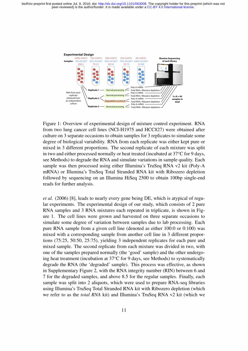
Figure 1: Overview of experimental design of mixture control experiment. RNAfrom two lung cancer cell lines (NCI-H1975 and HCC827) were obtained afterculture on 3 separate occasions to obtain samples for 3 replicates to simulate somedegree of biological variability. RNA from each replicate was either kept pure ormixed in 3 different proportions. The second replicate of each mixture was splitin two and either processed normally or heat treated (incubated at 37oC for 9 days,see Methods) to degrade the RNA and simulate variations in sample quality. Eachsample was then processed using either Illumina’s TruSeq RNA v2 kit (Poly-AmRNA) or Illumina’s TruSeq Total Stranded RNA kit with Ribozero depletionfollowed by sequencing on an Illumina HiSeq 2500 to obtain 100bp single-endreads for further analysis.

et al. (2006) [8], leads to nearly every gene being DE, which is atypical of regu-lar experiments. The experimental design of our study, which consists of 2 pureRNA samples and 3 RNA mixtures each repeated in triplicate, is shown in Fig-ure 1. The cell lines were grown and harvested on three separate occasions tosimulate some degree of variation between samples due to lab processing. Eachpure RNA sample from a given cell line (denoted as either 100:0 or 0:100) wasmixed with a corresponding sample from another cell line in 3 different propor-tions (75:25, 50:50, 25:75), yielding 3 independent replicates for each pure andmixed sample. The second replicate from each mixture was divided in two, withone of the samples prepared normally (the ‘good’ sample) and the other undergo-ing heat treatment (incubation at 37oC for 9 days, see Methods) to systematicallydegrade the RNA (the ‘degraded’ sample). This process was effective, as shownin Supplementary Figure 2, with the RNA integrity number (RIN) between 6 and7 for the degraded samples, and above 8.5 for the regular samples. Finally, eachsample was split into 2 aliquots, which were used to prepare RNA-seq librariesusing Illumina’s TruSeq Total Stranded RNA kit with Ribozero depletion (whichwe refer to as the total RNA kit) and Illumina’s TruSeq RNA v2 kit (which we

11

.CC-BY 4.0 International licensepeer-reviewed) is the author/funder. It is made available under aThe copyright holder for this preprint (which was not. http://dx.doi.org/10.1101/063008doi: bioRxiv preprint first posted online Jul. 9, 2016;

refer to as the poly-A mRNA kit). Libraries were sequenced as single-end 100bp reads on an Illumina HiSeq2500 instrument producing on average 50 millionreads per library (range 32 to 94 million). Reads from all samples were mapped tothe hg19 reference genome using the Subread alignment software [14]. Mappedreads were assigned using featureCounts [15] according to NCBI’s RefSeq hg19gene annotation.

Comparing read distribution by feature typeWe used a variety of strategies to annotate the reads depending on the analysis (seeMethods for a detailed description of the annotation strategies). To facilitate com-parison of the protocols in terms of read distribution across different genomic fea-tures, we reduced the reads mapped using the splice aware aligner Subjunc to their5’ position and assigned them to non-overlapping custom annotations restricted toeither exon, intron or intergenic regions (UTR regions were considered as exons).Genomic feature mapping statistics for all replicate 2 samples are shown in Figure2A. Interestingly, the poly-A mRNA and total RNA kits show greatest differencesin terms of reads mapping to introns, which come at the expense of exonic reads.The levels are similar between the degraded and good samples within each proto-col, with differences of a few percent at most. The poly-A libraries tend to capturemature poly-adenylated RNA which had undergone splicing, while the total RNAprotocol captures both mature and pre-messenger RNA alike, which is reflected inthe higher proportion of intronic reads in the latter. These results are similar to thepercentages reported in Zhao et al. (2014) [28], although we observe a slightlyhigher proportion of intronic reads in our data.

In order to compare the protocols with regard to read distribution across dif-ferent RNA classes, we used the gene-level exon counts (default featureCountsbehaviour) obtained from Subjunc aligned data and annotated them according tothe gene type information available with the annotation. The percentage of readsassigned to each type for all replicate 2 samples is shown in Figure 2B. Consistentwith the protocol design, the Total RNA method is able to recover a greater pro-portion of reads from non-coding (ncRNAs), small nuclear (snRNAs) and smallnucleolar (snoRNAs) RNA species compared to the poly-A mRNA kit (see Sup-plementary Figure 3 for results per RNA class). Across all samples, the percentageof reads mapping to ribosomal RNAs (rRNAs) was marginally lower for the totalRNA protocol compared to the poly-A mRNA kit (Supplementary Figure 3), in-dicating that the Ribozero depletion used to deplete rRNAs in the former samplepreparation method was highly effective, as previously reported [29, 28].

To assess data quality experiment-wide, we generated MDS plots from thegene-wise log2 counts per million (log-CPM) (Figure 2C-D). This display clearlyseparates the samples by mixture proportion, with increasing concentration of

12

.CC-BY 4.0 International licensepeer-reviewed) is the author/funder. It is made available under aThe copyright holder for this preprint (which was not. http://dx.doi.org/10.1101/063008doi: bioRxiv preprint first posted online Jul. 9, 2016;

Unmapped ReadsIntergenic ReadsIntronic ReadsExonic Reads

ncRNAsnRNAunknownpseudogenesnoRNArRNAother

Sample Sample

R2.

100

mR

NA

R2.

075

mR

NA

R2.

050

mR

NA

R2.

025

mR

NA

R2.

000

mR

NA

R2D

.100

mR

NA

R2D

.075

mR

NA

R2D

.050

mR

NA

R2D

.025

mR

NA

R2D

.000

mR

NA

R2.

100

Tota

lR

2.07

5 To

tal

R2.

050

Tota

lR

2.02

5 To

tal

R2.

000

Tota

lR

2D.1

00 T

otal

R2D

.075

Tot

alR

2D.0

50 T

otal

R2D

.025

Tot

alR

2D.0

00 T

otal

Proportion of reads mapped to thegenomic features with subjunc aligner

0

20

40

60

80

100

Perc

enta

ge

(A) Percentage of reads mapping todifferent genomic features

R2.

100

mR

NA

R2.

075

mR

NA

R2.

050

mR

NA

R2.

025

mR

NA

R2.

000

mR

NA

R2D

.100

mR

NA

R2D

.075

mR

NA

R2D

.050

mR

NA

R2D

.025

mR

NA

R2D

.000

mR

NA

R2.

100

Tota

lR

2.07

5 To

tal

R2.

050

Tota

lR

2.02

5 To

tal

R2.

000

Tota

lR

2D.1

00 T

otal

R2D

.075

Tot

alR

2D.0

50 T

otal

R2D

.025

Tot

alR

2D.0

00 T

otal

% of reads mapping to a particular gene type

% o

f tot

al n

umbe

r of r

eads

ass

igne

d to

gen

es

0

20

40

60

80

100

Perc

enta

ge

(B) Percentage of reads mapping todifferent gene types

●

● ●

●

●●

●●

●

●

●

●●

●

●

0

0

Pol

●

●●

●

●●

●●

●

●●

●●

●

●

0

0

T(C) MDS plot for Poly-A mRNA data (D) MDS plot for Total RNA data

Figure 2: Overview of data quality of mixture control experiment. (A) Mappingstatistics of reads assigned to different genomic features for all replicate 2 sam-ples (includes both intact (labels that begin R2) and degraded (labels that beginR2D) RNA samples). The percentages that could be assigned to exons, introns,intergenic regions or were unmapped are shown in different colours. (B) Mappingstatistics of reads assigned to different classes of RNA for all replicate 2 samples.This figure breaks down the gene-level exon reads from panel B according toNCBI’s gene type annotation. Multidimensional scaling plot of poly-A RNA (C)and total RNA (D) experiments showing similarities and dissimilarities betweenlibraries. Distances on the plot correspond to the leading fold-change, which is theaverage (root-mean-square) log2fold-change for the 500 genes most divergent be-tween each pair of samples. Libraries are coloured by mixture proportions, wherecircles represent good samples and triangles represent degraded samples.

NCI-H1975 indicated from left to right in dimension 1 and pure samples (100:0and 0:100) separating from the mixed samples (75:25, 50:50, 25:75) in dimension2 in both poly-A mRNA and total RNA data sets. For the poly-A mRNA data(Figure 2C), the replicate samples cluster less tightly, with the degraded samplesseparating slightly from the non-degraded samples for most mixtures. Samplesfrom the total RNA data (Figure 2D) on the other hand tend to cluster more tightly.

Exploiting signal from the mixture design genome-wideWe next inspect the typical FCs for the total RNA data using a mean-differenceplot from 3 pair-wise comparisons (100vs000, 050vs000 and 025vs000) to visu-alise the attenuation in signal that occurs as the RNA samples compared becomemore similar. Figure 3A shows the most extreme results, with average log2-fold-changes (log-FCs) (y-axis) versus average expression (x-axis) for the pure samples(100:0 versus 0:100, denoted 100vs000). The FCs cover a wide dynamic rangeand are symmetric about the log-FC = 0 (no change) line. When samples moresimilar in RNA composition are compared, the log-FCs are compressed and asym-metric (Figures 3B and 3C). Looking at the log-CPM-values at each mixture pro-portion for 3 representative genes (Figure 3D-F), we see the dose-response across

13

.CC-BY 4.0 International licensepeer-reviewed) is the author/funder. It is made available under aThe copyright holder for this preprint (which was not. http://dx.doi.org/10.1101/063008doi: bioRxiv preprint first posted online Jul. 9, 2016;

0.0 0.2 0.4 0.6 0.8 1.0

−6−5

−4−3

−2−1

01

(D) DAND5

Mixture proportion

log(

coun

t-per

-mill

ion)

●

● ●●

●

●

●

●

●

●

●

●

●

●

●

0.0 0.2 0.4 0.6 0.8 1.0

−2−1

01

23

45

(E) WASH7P

Mixture proportion

log(

coun

t-per

-mill

ion)

●● ●

●●

●

●

●●

●

●

●

●●

●

0.0 0.2 0.4 0.6 0.8 1.0

34

56

78

910

(F) EREG

Mixture proportion

log(

coun

t-per

-mill

ion)

●

●

●

●

●

●

●

●

●

●

●

●

●

●

●

●●

●

●●●

● ●

●●

●

●

●

●

●

●

●

●

●

●

●

●

●

●

●

●

●

●

●

●

●

●

●

●

●

●

●

●

●

●

●●

●

●

●

●

●●●

●

●

●

●

●

●●

●

●

●

●

●

●

● ●

●

●●●● ●

●

●

●

●

●

●

●

●

●

●●

●

●

●

●●

●

●

●

●

●

●

●

●

●

●

●

●

●

●

●

●●

●

●

●

●●

●

●

●

●

●

●

●

●●

●

●

●

●

●

●

●

●

●

●

●

●

●

●●●

●

●

●

●

●

●

●

●

●

●

●

● ●

●

●

●

●

●

●

●

●

●

●

●

●

●

●

●

●

●

●

●

●

●

●

●

●

●

●

●

●

●

●

●

●●

●●

●

●

●

●

●

●

●

●

●

●

●

●

● ●

●

●

●

●

●

●●

●

●

●

●●

●

●

●●

●

●

●

● ●

●

●

●

●

●

●

●●

●●

●

●

●

●●

●

●

●

●

●

●●

●

●

●

●●

●

●

●

●●

●

●

●

●

●

●

●●

●

●

●

●

●

●

●

●

●

●●

●

●

●

●

●

●

●

●

●

●

●

● ●●

●

●●

●●

●

●

● ●

●

●●

●

●

●

●●

●

●

●●

●

●

●

●

●

●

●

●

●

●

●

●

●

●

●

●

●

●

●

●

●

●

●●

●●

●

●●

●

●

●

●

●

● ●

●

●

●

●

●

●●

●●

●

●

●

●●

●●

● ●

●

●

●

●●

●

●

●

●

●

●

●

●

●

●

●

●

●

●

●

●

●

●

●

●

●

●

●

●

●

●

●

●

●●

●

●

●

● ●●

●

●●

● ●

●

●

●

●

●

●

●●

●

●

●

●

● ●

●

●

● ●

●

●

●

●

●

●●

●

●

●

●

●

●

●

●

●

●

●● ●

● ●

●

●

●

●●

●

●

●

●

●

●

●

●

●●

●

●

●

●

●●

●

●●

●

●

● ●

●

●●

●

●

●

●●●

●

●

●

●

●

●

●●

●

●

●●

●

●●

●

●

●

●

●

●●● ●

●

●

●

●

● ●

●

●

●

●

●

●

●

●

●

●

●

●

●

●

●

●

●

●

●

●

●

●

●

●

●

●

●

●

●

●

●

●

●

●●

● ●

●

●

●●

●●

●

●

●

●

●

●

●●

●

●

●

●● ●

●●●

●●

●

●

●● ●

●

●●

●

●

●

●

●

●

●

●

●

●●

●

●

●

●

●

●●●

● ●

●

●

●

●

●

●

●

●●

●

●

●

●

●

●●

●

●

●

●

●

●

●

●

●

●

●

●

● ●●

●●●

●

●

●

●

●

●

●

●

●

●

●

●

●

●

●

●

●

●

●●

●●

●

●●

●

●●

●

●

●

●

●

●

●

●

●

●

●

●

● ●

●

●● ●

●●

●

●

●

●

●

●●

●

●

●

●

●

●

●

●●

●

●

● ●

●

●

●

●●

●

●

●

● ●●

●

●

●

●

●

●●

●

●

●

●●●

●●

●●

●

●●

●

●

●

●

●

●

●

●●

●

● ●

●

●

●

●

●

●

●

●

●

●●

●

●

●

●

●

● ●

●

●●

●

●●●

●

●

●

●

●

●

●

●● ●

●●

●

●

●

● ●

●●

●●

●

●

●

●

●●

●

●

●

●

●●

●

● ●

●

●

●●●

●●

●

●

●

●●

●

●

●

●

●

●

●

●

●

●

●

●

●

●

●

●

●

●

●

●● ●

●

●

●

●

●●

●

●●

●

●

●

●

●● ●●

●●

●

●

●●

●●

●●

●

●

●

●

●●

●●

●

●

●

●●

●

●

●

●

●●

●

●

●

●

●

●●

●

●

●

●

●●

●

●

●

●●

●

●

●

●

●

●

●

●

●

●

●

●

●● ●

●●

●

●

●

●●

●

●

●

●●

●

●

●●

●●

●●

●

●

●

●

●

●

●

●●

●

●

●

●

●

●

●

●

●

●

●

●

●

●

●

●●

●

●

●

●

●

●●

●

●

●

●

●●

● ●

●

●

●●

●

●

●

●

●

●

●●

●●

●●

●

●●

●

●

●

●

●

●

●●

●

●

●

●

●

●

●

●

●

●

●●

● ●

●

●

●

●

●

●

●

●●

●

●

●

●

●

●●

●

●

●

●

●

●●

●

●

●

●

●●

●

●●●

●

●

●●

●

●

●

●

●

●

●

●●

●

●

●

●

●

●

●●

● ●

●

●

●

●

●●●●

●

●

●

●

●

●

●

●

●●

●●

●

●●

●

●

●●

●

●

●

●

●

●

●

●

●

●

●

●

●

●

●

●

●

●

●

●

●

●

●

●

●●

●

●

●

●

●

●

●

●

● ●

●

●

●

●

●

●

●

●

● ●●

●

●

●

●

●

●

●

●●

●

●

●

●

●

●

●

●

●

●

●

●

● ●

●

●

●

●

●

●

●

● ●

●

● ●●

●

●

●●

●

●

●

●

●

●

●●

●

●

●

●

●●

●

●●

●

●

●

●

●

●

●

●●

●

●

●

●●

●

●●

●

●

●●

●

●

●

●●

●●

●

●

●

●●

●

●

●

●●

●

●

●

●

●

●

●●

●

●

●

●

●

●

●●

●●●

●●

●

●

●

●●

●

●

●

●

●●

●

●

●

●

●

●

●

●●

● ●●

●

●

●

●

●

●

●

●

●

●

●

●

●

●

●

●

●

●

●

●

●

●

● ●●

●●●

●

●

●

●●

●

●

●

●

●

●● ●●

● ●

●

●

●

●

●●

●

●

●

●

●

●

●

●

●

●

●

●

●

●

●

● ●●

●

● ●●

●●●

●

●

●

●

● ●

●

●

●

●● ●

●

●

●

●

●

●

●

●

●●

●●

●●

●

●

●

● ●●

●

●

●

● ●

●

●

●● ●

●

●

●

●

●

●

●

●

●

●

●

●

● ●

●

●

●●●

●

●●

●

●

●●●

●●● ●

●

●

●

● ●

●

●

●

●

●

●

●

●

●

●

●

●●

●

●

●

●

●

●●

●

●

●

●

●

●

●

●

●

●●

●

●

●

●

●●

●

●

●

●

●

●

● ●

●

●

●●

●

●

●

●

●

●

●

●

●

●

●

●

●●

●

●

●●

●●

●

●

●

●

●

●

●

●●

●

● ●

●

●

●

●

●

●

●

●●

●

●

●

●

●●

●

● ●

●

●

●●

●

●

●

●●●

●

●

●

●

●

●

●

●

●

●

●

●

●

●

●

●

●●

●

●

●

●

●

●

●

●

●

●

●

●

●

●

●

●

●●●

●

● ●

●

●●

●

●

●

●

●

●

●●●

●

●●

●

●

●

●

●

●

●

●

●

●

●

●

●

●

●

●

●

●

●

●

●

●●

●

●

●

●

●●

●

●

●

●●

●

●

●

●

●

●

●

● ●

●●

●

●

●

●

●●

●

●

●

●●

●

●

●

●

●

●●

●

●

●

●

●

●

●

●

●●

●

● ●

●

●

●

●

●

●

●

●

●

●

●

●

●

● ●

● ●●

●●

●

●

●

●

●

●

●

●

●

●

●

●

●

●

●

●

●

●

●

●

●

●● ●

●

●

●

●

●

●●

●

●

●

●

●

●

●

●

●

●

●

●

●

● ●

●

●

●●●●●

●

●

●

●

●

●

●

●

●

●

●

●●

●●

●

●

●

●

●

●

●●

●

●

● ●●

●

●●

●

●

●●

●

●

●●

●

●

●

●

●

●

●

●

●

●

●

●

●

●

●

●

●

●

●

●

●

●

●

●

●

●

●

● ●

●

●●

●

●

●

●

●

●

●

●●

●

●

●

●

●●

●

●

●

●

●

●

●

●

●

●

● ●

●

●

●

●●

●

●

●

●●

●

●

●●

●

●

●

●

●

●

●

●

●

●

●●

●

●

● ● ●● ●

●

●

●

●

●

●●

●

●

●●

●

●

●

●

●

●

●

●

●

●

●

●

●

●● ●●

●

●

●

●

●

●

●

●

●

●

●

●

●

●

●

●

●

●

●

●

●

●

●

●

●

●

●

●●

●

●

●●

●

●

●

●

●

●

●

●

●

●

●

●●

●

●

●

●

●

● ● ●

●

●

●

●

●

●

●

●

●

●

●

●●

●

●

●

●●

●

●

●

●●

●

●

● ●●

●

●●

●●

●

● ●

●

●

●

●

●

●●

●

●

●●

●

●

●

●

●

●●

●

●

●

●

●

●

●

●

●● ●

●

●

●

●

●

●

● ●

●

●

●

●

●

●

●

●

●

●

●

●

●

●

●

● ●

●

●

●

●

●● ●

●

●

●

●

●

●

●

●

●●

●

●

●

●

●

●

●

●

●

●

●

●

● ●

●●

●

●

●

●

●●

●

●

●

●

●

●

●

●

●

●

●

●

●

●●

●

● ●

●●

●

●

●

●

●

●

●

●

●●

●

●

●

●

●

●

●●

●

●

●

●

●

● ●

●

●

●●

●

●

●

●

●

●●

●

●

●

●

●

●

●

●●

●●

●●●

●

●

●●

●

●

●

●

●

●

●

●

●

●●

● ●●

●

●

●

●

●

●

●

●

●

●

●

●

●

●

●

●

● ●

●●

●

● ●

●●

●

●

●

●

● ●●

●

●

●

●

●

●

●

●

●

●

●

●

●

●

●●

●●

●

●

●

●

●

● ●

●

●

●

●

●

●

●

●●

●

● ●

●

●

●●● ●

●

●

●

●

●

●

●

●

●

●

●

●

●

●

●

●

●●

●

●

●

●

●

●

●

●

●

●

●

●

●

●

●

●●

●

●

●

●●

●

●

●

●● ●

●

●

●

●

●●

●

●

●

●

●

●●

●●

●

●

●

●

●

●

●

●

●●●

●

●

●

●

●●

●

●

●

●

●

●

●

●

●●

●●

●

●

●●

●

●

●

●

●

●

●

●

●

●

●

●

●

●

●●

●

●●

●●●

●

●

●

●

●

●

●

●

●

●●

●●

●

●

●

●

●

●

●

●●

●

●

●

●

●●

●

●

●

●

●

●

●

●

●

●

●

●●

●●

●

●

●

●

●●

●●

●

● ●

●

●

●

●

●

●

●

●

●

●

●

●

●

●

●●

●

●

●

●

●●

●

●

●●

●

●

●

●

●

●●

●

●

●

●

●● ●

●

●

●

●

●

●

●

●

●●

●

●

●

●

●

●

●

●

●

●

●●

●

●●●●

●

●

●●

●

●

●●●

●

●

●

●

●

●

●

●

●

●

●

●

●●

●

●

●●●

●●

●

●

●

●

●

●●

●●

●

●

●

●●

●

●

●●

●

●

●

●

●

●

●

● ●●

●

●●● ●

●

●

●

●

●

●●

●

●

●

●

●

●●

●

●

●

●

●

●

●

●

●

●

●

● ●

●

●

●

●

●

●

●●

●

●

●

●

●

●

● ●

●

●

●

●

●

●

●

●

●●

●

●

●

●

●

●

●

●

●

●

●

●

●

●

●

●●●

●

●

●●

●

●

●

●

●

●

●●●

●

● ●

●

●

●

●

●

●●

●

● ●

●

●

●

●

● ●

●

●

●

●

●

●

●

●

●

●

●

●●

●

●

●

●

●

●

●●

●

●

●

●

●

●

●

●●

●●

●

●

●●

●

●

●

●●

●

●

●

●●

●

●

●

●

●

●

●

●

●

●

●

●

●

●

●●

●

●

●

●

●

●

●

●

●

●

●

●

●

● ●

●

●

●

●

●

●

●

●

●

●

●

●

●

●●●

●

●

●

●●

●

●●

●

●

●

●

●

●

●

●

●

●

●

●

●

●

●

●

●

●

●●

●

●

●

●●

●

●

●

●

●

●

●

●

●●

●

●

●

●

●

●

●

●●

●

●

●

●

●

●

●

●●

●

●●

●

●●

●

● ●

●●

●

●

●

●

● ●

●

●

●

●

●

●

●

●

●

●

●

●

●●

●

●

●

●

●

●

●

●

●

●

●

●●

●

●

●

●

●

●

● ●

●

●

●

●

●

●

●

● ●

●

●

●

●

●

●

●

●

●

●

●●

●

●

●●

●

● ●●

●

●

●

●

●

●

●

●

●

●

●

●

●

●

●

●●

● ●

●

●

●

●

●

●

●

●

●

●●

●

●

●

●●

●

●

●

●

●

●

●●

●

●

●

●

●

●

●●

●

●

●

●

●

●

●

●●

●

●

●●

●

●

●

●

●

●

●

●

●

●

●

●

●

● ● ●

●

●

●

●

●

● ●●

●●

●

●

●

●

●

●●

●

●●

● ●

●

●●

●

●

●

●

●

●

●

●

●

●

●

●

● ●

●

●

●

●●

●

●

●

●

●

●

●

●

●

●

●

●

●

●

●

●●

●

●

●

●

●

●

●

●

●

●

●

●

●

●

●●● ●

●

●

●

●

●●

●

●

●

●

●

●

●

●

●

●

●●

●●

●

● ●

●

●●

●

● ●

●

●

●

●●

●●

●

●

●

●

●

● ●

●

●

●

●

●

●

●

●

●

●

●

●

●

●

●

●

●

●

●

●

●

●

●

●

●

●

●

●

●

●

●

●

●

●

●

●

●

●●

● ●

●●

●

●

● ●

●

●

●

●●

●●

●

●

●

●

●

●

●

●

●

●

●●

●

●

●

●

●●

●

● ●

●

●

●

●

●

●

●

●

●

●●

●

●

●

●

●

● ●●

●●

●

●

● ●

●

●

● ●●

●

●

●

●

●

●

●

●

●

●

●●●

●

●●

●●

●

●

●

●

●

●

●

●

●

●

●

●

●

●

●●

●

●

●

●

●

●

●

●

●

●

●

●

●●

●●

●●

●

●

●

●

●● ●●

●

●

●

●

●

●

●●

●

●●

●

● ●

●

●

●

●

●

●●

●

●●

●

●

●

●●

●

●

●●●

●

●

●

●●

●

●

●

●

●

● ●

●

●

●

●

●

●

●

●

●

●●

●

●

●●

●

●

●

●

●

●

●

●

●

●●

●

●

●●

●

●

●●

●

●

●

●

●●

●

●

●

●

●●

●

●

●

●●

●

●● ●

●

●●

●

●

●

●

●

●

●

●

●

●●●

●

●

●

●

●●●

●

●●●

●

●●

●

●

●

●

●●

●

●

●●

●

●

●

●

●

●

●

●

●● ●●

●

●

●

●

●

●

●

●

●

●●

●

●

●

●

●

●

●

●

●

●

●

●

● ●

●

●

●

●

●

●

●

●

●

●●

●

●

●

●

●

●

●

●

●

●

●

●●

●

●

●

●●

●

●

●

●

●

●

●

●

●

●

●

●

●

●

●

●●●

●

●

●

●

●

●●

●

●

●●

●

●

●

●●

●

●●

●

●

●

●

●

●

●

●●

●

●

●

●

●

●

●

●●

●

●

●

●●

●

●

●

●

●

●

●

●

●●

●●

●

●

●

●●●

●

●

●

●●

●

●

●

●

●

●●●●

●

●●

●

●

●

●

●

●

●

●●

●●

●

●

●

●●

●

●

●

●

●

●

●●

●

●

●●

●

● ●

●

●●

●

●

●●

●

●

●

●

●

●

●

●

●●

●

●

●

●

●

●

●

●

●

●

●

●

●

●●

●

●

●●

●

●

●

●

●

●●

●

●

●

●

●

●

●

●

●

●

●

●

●●●

●

●

●

●

●

●

●

● ●

●

● ●●

●

●

●●

●

●

●

●

●

●

●

●●

●●

●

●

●

●

●

●

●

●

●

●

●

●

●●

●●

●

●

●●

●

●

●●●

●

●●

●

●

●●

●

●●●

●

●

●

● ●

●

●

●

●

●

●

●●

●

● ●

●

●

●

●

●

●●●

●

● ●

●

●

●●●●

●

●

●

● ●

●

●

● ●

●

●

●

●

●

●

●

●

●

●

●

●

●

●

●

●

●

●

●

●

●

●

●

●

●● ●

●●

●

●

●

●

● ●

●

●

●

●●

●

●

●

●

●

● ●

●●

● ●

●

●

●

●

●

●

●

●

●●●●

●●

●

●

●

●

●

●

●●

●●

●

●

●

●

●

●

●●

●

●

●

●

●●

●

●●

●

●●● ●

●●

●●

●

●

●●

●

●

●

●●

●

●●●

●

●

●

●

●

●

●

●

●

● ●

●●

● ●

●

●

●●

●

●

●

●

●

●

●

●●

●

●

●

●

●

●

●●

●

●

●●

●

●

●

●

●●

●

●

●●

● ●

●

●●●

●

●

●

●●

●

●●

●

●

●

●

●

●

●

●

●

●●

●

●

●

●● ●

● ●●

●

●

●

●●

●

●

●

●

●

●

●

●

●

●●

●

●●

●

●

●

●

●

●

●

●

●

●

●

●

● ●

●

●

●●

●

●●● ●● ●

●

●

●

●

●

●

●

●●

●

●

●

●

●

●

●●

●

●

●

●

●

●

●

●●●

●

●

●

● ●

●

●

●●

●

●

●

●

●

●

●

●

●

●●●

●

●

●

●

●

●

●

●

●

●

●

●

●

●

● ●

●

●

●

●

●

● ●● ●

●

●

●

●

●

●

●

●

●

●

● ●● ●

●

●

●

●

●●

●

●

●

●

● ●

●

●●

●

●●

●

●

●

● ●

●

●

●●

●

●

●

●

●

●

●

●

●

●

●

●

●

●

●

●●

●●●

●●

●

●

●

●

●

●

●

●

●

●

●

●

●

●●

●

●

●

●

●

●

●

●●

●

●

●

●●

●

●

●

●

●

●

●

●

●

●

●

●

●

●

●

●●

●

●

●●

●●

●

●

●

●

●

●

●

●

●●

●

●

●●

●

●●

●

●

●

●

●

●

●

●●

●

●

●

●●

●●

●

●

●

●●

● ●●●

●●●

●

●

●●

●

●

●

●● ●

●

●

●

●

●

●

●

●

●

●

●●●

●● ●

●●

●●

●

●

●

●

●

●

●

●

●

●

●

●●

●●

●

●

●

●

● ●

●

●

●

●

●

●

●

●

●

●

●

●●

● ●

●

●●

●

●

●

●

●

●●

●

●

●

●

●●

●●

●

●

●●

●

●

●

●

●

●

●●

●

●

●

●

●

●

●

●

●

●

●

●

●

●

●

●

●●

●

●

●

●

●

●

●●

●

●●

●

●●

●

●

●

●●●

●

●

●

●

●

●

●

●

●

●●

●

●

●

●

●

●

●

●

●

●

●

●

●

●

●

●

●

●

●

●

●

●●

●

●●

●●

●●

●

●

●

●

●

●

●

●

●

●

●

●

●●

●

●●

●

●

●

●

●

●

●

●●

●●

●

●

●

●

●

●●

●●

●

●●● ●

●●

●●

●

●

●

●

●

●

●

●

●●

●

●

●

●

●●

●

●●

●●

●

●

●

●

●

●●

●

●

●●

●

●

●●

●

●

●

●

●

●

●

●●

●

●

●

●

●

●●

●●

●

●

●

●

●

●

●

●

●

●

●

●

●

●

●

●

●

●●

●

●

●

●

●

●

●

●

●●

●

● ●●

●

●●

●●●●

●

●●

●●

●

●

●

●

●

●

●

●

●

●

●

●

●

●

●

●

●

●

●

●

●

●

●●●

● ●●

●

●●

●

●

●

●

●

●●

●

●

●

● ●

●

●

●●●

●

●

●

●

●

●●●

●

●

●

●

●

●

●

●

●

●

●

●

●

●●

●

●

●

●

●

●

●

●●

●

●●

●

●

●

●

●

●

●

● ●

●

●

● ●

●

●

●●

●

●

●

●

●

●

●

●

●

●

●

●

●●●

●●

●

●

●

●

●

●

●

●

●

●

●

●

●

●

●

●

●

●●●●●●

●

●●

● ●

●●

●●

●

●

●

●

●

●

●

●

●

●●

●

●

●●

●

●

●

●

●

●

●

●

●

●

●

●

●

●

●

●●

●

●●

●

● ●

●

●

●

●●●

●

●

●

●

●

●●●

●

●

●

●

●

●

●

●

●●

●●

●

●

●

●

● ●●

●

●

●

●

●

●

●

●

● ●

●

●

●

●

●

●

●

●

●

●

●

●

●

●

●

●

●

●

●

●

●

●

●

●

●●

●

●

●●

●

●

●

●●●

●

●

●

●

●

●

●

●

●

●

●

●

●

●●

●

●

●

●

●

●●

●

●

●

●

●

●

●●

●

●●

●

●

●●

●●

●

●

●

●

●

●

●

●

●

●

●

●

●

●

● ●

●

●

●

●●

●

●

●

●

●

●

●●

●

●

●

●

●

●●

●

●

●

●

●

● ●

●

●

●

●

●

● ●

●

●

●●

●

●

●●

●

●

●

●

●

●

●

●

●

●

●

●

●

●

●

●

●

●

●

●●●

●●●

●

●

●

●

● ●●

●

●

●●

●

●

●

●

●

●

●

●

●

●●

●

●

●

●●

●●

●

●

●

●

●

●

●

●

●

●●

●

●

●

●●

●

●

●

●●

●●

●

●

●

●

●

●

●

●

●●

●

●

●

●

●

●

●●

●

●

●

●

●

●

●

●

●

●

●

●

●

●

●

●

●

●

●●

●

●

●

●

●

●

●

●

●

●

●

●

●

●

●

●

●

●●●●●●

●

●

●

●

●

●

●

●

●●

●

●

●

●

●

●

●●

●

●

●

● ●●

●

●

●

●

●

●●

●

●●

●

●

●

●

●

●

●●

●

●

●

●

●

●

●

●●

●

●

●

●

●

●

●

●

●

●

●

●

●

●●●

●

●●●

●

●

●

●

●

●

●

●●

●

●

●

●●

●

●

●

●

●

●

●

●●● ●

●

●

●

●●

●

●

●

●

●●

●

●

●●●

●

●

●

●

●

●

●●

● ●

●

●

●

● ●

●●

●

●

●

●

●

●

●

●

●

●

●

●●●

●

●●

●

●

●

●

●

●

●

●●

●

●●

●

●

●

●

●

●●

●

●

●

●

●

●

●

●

●

●

●

●

●●

●

●

●

●●

●

●

●

●

●

●

●

●

●●

●

●

●●

●

●

●

●

●

●

●

●

●

●

●

●

●

●

●●

●

●

●

●

●●

● ●

●

●

●

●

●

●

●

●

●

● ●

●

●

●

●

●

●

●

●

●

●●

●●

●●

●

●

●

●

●●

●

●

●

●

●

●●● ●●

●

●

●

●

●

●

●

●

●

●

●●●●

●●

●

●

● ●

●

●

●

●

●

●

●

●

●

●

●

●

●●

●

●

●

●●

●

●

●

●●

●●

●

●

●

●

●

●

●●

●

●

●

●●

●●

●

●

●

●

●

●

●

●

●

●

●

●

●

●

●

●

●

●

●

●

●

●●

●●

●

●●●

●

●

●

●

●●

●

●●

●●●

●

●●

●

●

●●●

●●

●

●●●

●

●

●

●

●

●

●

●●● ●●

●●

●

●

● ●

●●●

●

●

●

●

●

●

●

●

●

●

●

●●

●

● ●●

●

●

●●●●

●

●

●

●

●

●

●

●●●●

●

●

●

●●

●

● ●

●●

●

●

●

●

●

●●

●

●●

●

●

●●

●

●

●

●

●

●

●

●

●

●

●

●

●

●

●

●●

●

●●

●●

●

●

●

●

●

●

●

●

●

●

●

●

●

●

●

●

●

●

●●

●

●

●

●

●

●

●

●

●

●

●

●

●

●

●

●●

●

●

●

●●

●

● ●

●

●

● ●

●

●

●

●

●

●

●

●

●●

●

●●

●●

●

●

●

●●

●●

●

●

●

●

●

●

●

●

● ●●

●

●

●

●

●

●

●●

●

●

●

●

●

●

●

●

●●●

●

●

●

●

●

●

●●

● ●● ●

●

●

●

●

●

●

●

●

●

●

●

●

●

●●

●●

●

●

●

●

●

●

●

● ●●

●

●

●●

●

●

● ●

●

●

●

●●

●

●●

●

●

●●

● ●

●

●

●

●●

● ●

●

●

●

●●

●

●●

●

●

●

●●

●

●

●

●●

●●

●

●

●

●

●

●

●●

●

●

●

●

●●

●●

●

●

●

●

●

●

●●

●

●●

●

●

●

●

●

●

● ●

●

●

●

●

●

●

●

●

●

●

●

●

●

●

●

●

●

●● ●

●

●

●

●

●

●

●

●●

●

●

●●

●

●●

●

●

●

●

●

●

● ●

●

●

● ●

●

●

●

●

●

●

●

●●●

●

●

●

●

●

●

●

●

●

●

●

●

●

●

●

●●

●

●

●

●

●

●● ●

●

●

●

●

●

●

●

●

●

● ●

●

●

●

●

●

●

●

●

●

●●

●●

●

●

●

●

●

●

●

●

●

●

●

●

●

●

●

●

●

●

●

●

●

●

●

●●

●

●

●

●

●

●●

●

●

●●

●●

●

●

●

●

●

●

●

●

●

●

●

●

●

●

●

●

●●

●

●

●●

●

●

●

●

●

●

●

●

●●

●

●

●

●

●

●

●

●

●●

●

●

●

●●

●

●

●

●

●

●

●

●● ●

●

●

●

●

●

● ● ●

●●

●●

●

●

●

●

●

●

●

●

●

●

●●

●

●

●

●

● ●

●

●

●

●

●

●

●

●

●●

●

●

●

●

●

●

●●

●●

●

●

●

●

●

●

● ●

●● ●

●

●

●

●

●

● ●

●

●

●

●

●●

●

●

●

●

●

●

●

●

●

●

●

●●● ●

●

●

●

●

●

●●

●

●

●

●

●

●●

●

●

●

●

●

●

●

●●

●

●●

●

●

●

●

●

●●

●

●

●

●

●

●

●● ●

●●●

●

●

●

●●

●

●

●

●●

●●●●●

●

●

●

●

●

●

●

●

●

●

●

●

●

●

●

●

●●●

●

●

● ●

●

●

●

●

●

●

●●●●

●

●●

●

●

●

●

●

●● ●●

●

●

●

●

●

●

●●●●●

●

●

●

●

●

●

●

● ●

●

●●

●● ● ●●

●

●●●●●●

●●●

●

●●●●●●

●

●

●

●

●

●

● ●

●

●

●

●●

●

●●

●

●

●

●

●

●

●

●

●

●

●

●

●

●

●

●

●●

●●

●●

●

●

●

●

●

●

●

●

●

●●●●

●

●

●

●

●

●

●

●●

●●

●

●

●

●

●

●

●

●

●

●

●

●●

●

●●

●

●

●●●

●

●

●

●

●

● ●

●●

●

●

●

●

●

●●

●

●

●

●●

●

●

●●●

●

●

●●●

●

●●

●

●

●●

●

●

●

●

●

●

●

●

●

● ●

●

●

●

●

●

●

●

●●

● ●

●

●

●

●

●

●●

●

●

●●

●

●

●

●

●

●

●

●

●

●

● ● ●

●

●

●

●

●

●●

●●●

●

●

●

●

●

● ●

● ●●

●

●

● ●●

●

●●

●●

●

●

● ●

●●

●

●

●

●

●●●

●

●

● ●

●

●

●

●

●

●

●

●

●

●

●

●●

●

●●

● ●

● ●●

●

●

●

●●

●● ●●

●

●

●

●

●

●

●

●

●●● ●

●

●

●

● ●●●

●

●

●

●

●

●

●

●

●●●

●

●

●●

●

●

●

● ●

●

●

●

●

●

●

●

●

●

●●●

●

●●

●●

●

●●

●●

●

●

●

●

●

●

●

●●

●

●

●●

●

●●

●

●

●● ●

●

●

●

●

●

●●

●

●

● ●

●

●

●

●

●

●

●●

●

●●●

●●

●

●

●

●

●

●●

●

●

●●

●

●

●

●●

●

●

●

●●

●

●

●

●

●

●

●

●

●

●

● ●

●

●

●

●

●

● ●●●

●●

●●●

●

●

●●

●

●

● ●

●

●●

●

●

●●

●

●

● ●

●

●

●

● ●

●

●

●

●

●

●

●

●

●

●

●

●

●

●

●

●

●●

●

●●

●

●

●

●

●●

●

●

●●

●

●

●

●

●

●

●

●

●

●

●

●

●

●

●

●

●●

●

●

●

●

●

●

●

●

●

●●

●

●

●●●

●

●

● ●

●

●

●

●●

●

●●

●

●

●

● ●

●

●

●

●

●

●

●●

●●

●

●

●

●

●●

●

●

●

●

●

●

●

●

●

●

●

●

●

●

●●

●

●

●

●

●

●

●

●

●●

●

●

●

●

●●

●

●

●

●

●

●●

●

●●

●

●

●

●

●

●

●

●

●

●

●

●

●●

●

●

●

●

●

●

●

●

●●●

●

●●●●●●●●

●

●●

●

●

●

●

●●●

●●●●●

●

●

●

●

●

●

●

●

●●

●

●

●

●

●●●●

●

●

●●

●

●

●

●

●●

●●●

●

●

● ●

●

●

●

●

●

●

●

●

●

●●

●

●

●●

●

●

●

●

●

●

●

●

●

●

●

●

●

● ●

●

●

●

●

●

●

●

●

●

●

●

●

●

●●

●

●

●

●

●

●

●

●

●

●

●

●

● ●

●

●

●

●

●●

●

●

●

●

●

●

●

●

●

●

●

●

●●

●

●●●

●

●

●

●

●

●

●

●●

●

●

●

●

●

●

●●

●

●

●

●

●●●●

●

●

●

●

●

●●

●●

●

●

●

●

●

●

●

●

●

●

●

●

●

●

●

●

●

●

●

●●

●

●●

●

●

●

●●

●

●

●

●

●

●

●

●

●

●●●● ●

● ●

●

●●

●

●

●

●

●

●

●●

●

●●●●●●

●

●●

●

● ●

●

●

●

●

●●

●

● ●

●

●

●

●

●

●

●

●

●●

●

●

●

●

●

●

●

●

●

●

●

●

●●

●

●●

●

●

●

●

●

●

●

●●●

●

●

●

●

●

●

●

●

●

●

●

●

●●

●

●

●

●

●

●

●●

●

●

●

●●

●●

●

●

●

●

●

●●

●

●

●

●●

●

●

●

●

●●

●

●●●

●

●●

●

●

●

●

●

●

●

●●

●

●

●

● ●

●

●●

●●

●

●

●

●

●

●

●

●

●

●●

●

●

●

●

●

●●

●

●

●

●

●●

●

●

●

●

● ●●

●

●

●

●

●●

●

●

●●

●

●

●●●

●●

●

●

●

●

●

●

●

●

●

●

●

●

●

●

●

●●

●

●

●

●

● ●

●

●

●

●

●● ●

●●

●

●

●

●

●

●

●

●

●

●

●

●

●

●

●

●

●

●

●

●

●

●

●

●●

●

●

●

●● ●●

●

●

●

●

●

●

●●

● ●

●

●

●

● ●

●

●

●

●

●

●

● ●

●

●

●

●

●

●

●

●

●

●

●

●

●

●

●

●

●

●

●

●

●

●

●

●

● ●

●

●

●

●

●

●

● ●

●

●

●

●

●

●

●

●●

●

●

●●●

●

●

●●

●

●●●

●

●

●

● ●

●

●

●

●

●

● ●

●

●

●

●

●

●

●

●

●

●

●

●●

●

●

●

●

●●

●

●●

●

●

●

●

●

●●●

●

●

●

●

●

●

●

●

●

●

●●

●

●

●

●

●

●

●

●

●

●

●

●

●

●

●

●●

●

●●

●

●●

●

●

●● ●

●

●●

●●

●

●

●

●

●

●

●

●●

●●

●

● ●

●

●

●

●

●

●

●●

●

●

●

●

●●

●● ●

●●

●

●

●

●

●

●

●

●

●

●

●●●

●●

●

●

●

●

●

●

●

●

●

●

●

●

●

●

●

●

●

●

●

●

●

●

●

● ●

●

●●

●

●

●●

● ●

●

●

●

●

●●

● ●

●

●

●●

●

●

● ●

●

●

●

●

●

●

●

●

●

●

●●

●

●

●

●

●

●●

●

●

●●

●

●

●●

●

●

●

●

●

●

●

●

●

●

●

●

●

●

●

●

●

●

●

●

●●

●

●

●

●

●

●

●

●

●

● ●

●

●

● ●

●

●

●

●

●

●●

●

●

●

●

●

●

●

●

●

●

●

●●

●

● ●

●

●

●

●

●

●

●

●●

●

●●

●

●

● ●

●●

●

●●

●

●

●

●●●

●

●

●

●

●●

●

●●●

●

●

●

●

●

●●

● ●

●

●●

●

●

●

●

●

●

●

●

●

●●

●

●

●

●

●

●●

●

●

●

●

●

●

●●

●

●

●

●

●

● ●

●

●

●

●●

●

●●

●

●

●●

●

●

●

●

●

●

●

●

●

●

●

●

●

●

●

●

●

● ●

●

●

●●

●

●

●

●

● ●

●

●

●

●●

● ●

●

●

●

●

●

●

●

●

●

●●

●

●

●

●

●●

●

●

● ●

●

●●

●●●

●

●

●

●

●

●

●

●●

●

●

●●

●

●

●●

●

●

●

●●

●

●

●

●

●

●

●

●

●

●●

●

●

●

●

●

●●

●

●

●

●●

●●

●

●

●

●

●

●

●

●

●

●●●

●

●

●

●●

●

●

●

●

●

●●

● ●

●

●

●

●

●

●

●

●●

●

●

●

●

●

●

●

●●● ●

●●

●●

●

●

●

●

●

●

●

●

●

●

●

●

●

●

●

●

●

●

●

●

●

●

●

●

●

●

●

●

●● ●

●

●

●●

●

●

●

● ●

●●

●●

●

●

●

●

●

●

●

●●

●

● ●●

●

●

●

●

●

●

●

●

●

●

●

●●

●

●

●

●

●

●

●

●

●●

●●

●

●●

●●

●

●

●

●●

●

●●

●

●

●

●

●

●

●●

●

●

● ●●

●

●

●

●

●

●

●

●

●

●

●

●●

●

●

●

●

●

●

●●

●

●● ●

●

● ●

●

●

● ●

●

●●

●

●

●

●

●

●

●

●

●

●

●

●

●

● ●

●

●●

●

●●

●

●

●

●

●

●

●

●

●

●● ●

●

●

●

●●●

●

●

●●●

●

●

●

●

●

●

●

●●

●

●●

●

●

●

●

●

●●

●

●

●

●●

●

●●

●

●

●

●

●

●

●

●

●

●

●

●

●

●

●

●

●

●

●

●

●

●

●

●

●

●●

●

●●

●●

●

●

● ●

●

●

●

●●

●

●●

●

●

●

●

●

●

●

●

●●

●

●

●

●

●

●

●

●

●●

●

●

●

●

● ●●

●

●

●

●

●

●

●●

●

●

●

●

●

●

●

●

●

●

●

●

● ●

●●

●

●

●

●

●

●

●

●

●

●●

●

●

● ●

●

●

●

●

●

●

●

●

● ●●

●

●

●

●

●●

●

●

●

●●

●

●

● ●

●

●

●

●

●

● ●

●

●

●

●

●

●

●

●

●

●

●

●

●●●

●●

●

●

●

●

●

●

●

●

●●●

●●

●

●

●

●

●

●

● ●

●

●

●

●

●●

●

●

●●

●

●

●

●

●

●

●

●

●

●

●●

● ●

●

●

●

●

●

●

●

●

● ●●

●●

●

●

●

●

●●

●

●

●

●

●●●

●

●

● ●●

●

●

●

●●

●

●

●

●

●

●

●

●

●

●

●

● ●

●

●●

●

●●

●

●

●

●

●

●●

●

●

●

●

●

●

●

●

●

●

●

●

●

●

●

●

●

●

●

●

●

●●

●

●

●

●

●

●

●

●

●

●

●

●

●

●

●

●

●

●

●

●

●

●

●

●

●

●

●

●●

●

●

● ●

●

●●

●

●

●

●

●●

●

●

●

●

●

●

●●

●

●●

●

●

●

●

●●

●

●

●●

●●

●

●

●

●

●

●

●

●

●

●

●

●

●

●

●

●

●

●

●

●●

●

●

●

●

●

●

●●

●

●

●●

●

●

●

●

●

●●

●

●

●

●

●

●

●

●

●

●

●

●

●●

●

●

●

●

●

●●

●

●●

●●

●

●

● ●

●●

●

●

●

●

●

●

●

●●

●

●

●

●

●

●

●

●

●

●

●●

●

●

●

●

●●●

●

●

●

●●

●

●

●

●

●●

●●

●●

●

●

●

●

●● ●

●

●

●

●

●

●

●

●●

●

●

●

●

●

●

●

●

●

●

● ●

●

●●● ●●

●

●

●

●●

●

●

●

●

●●

●

●

●

●

●

●

●

●

●

●

●●

●

●

●

●

●

●

●

●

●

●

●

●

●

●

●●

●

●

●

●

●

●

● ●

●

●

●

●

●

●

●●

●

●

●

●

●

●

●

●

●

●●

●● ●

●

●

●

●

●

●

●

●

●

●●

●

●

●

●

●

●

●

●

●

●

●

●

●

●

●

●

●

●

●

●

●

●

●

●

●

●

● ●

●

●

●

●

●

●●

●●●

●

●

●●

●

●

●

●

●

●●

●

● ●

●

●

●

● ●

●

●

●

●

●

●

●

●

●

●

● ●

●● ●

●

●

●

●●

●●

● ●

●

●

●●

●

●●

●

●●

●

●

●

●

●

●

● ●

●

●

●

●● ●

●

●●

●

●

●

●

●●

●●

●

●

●

●

●

● ●

●

●

●

●

●●

●

●

●

●

●

●

●

●

●

●

●

●

●

●●

● ●

●●

●●●

●

●●

●

●●

●

●

●

●●

● ●

●

●

●

●

●

●

●●

●

●

●

●

●

●

●

●●

●

●

●

●

●

●

●

●

●

●

●

●

●

●

●

●

● ● ●

●

●

●

●

●

●

●

●

●

●

●

●●

●

●

●● ●

●

●●

●

●

●●

●

●

●

●

●

●

●

●

●

●●

●

●

●●

●

●

●

●

●

●

●●

●

●

●

●

●

●

●●

●

●

●

●

●

●

●

●

●

●

●●

● ● ●

●

●

●

●

●

●

●

●

●

●

●

● ●

●

●

●

●

●

●

●

●

●

●

●●

●●

●

●

●●

●

●●

●

●

●

●

●

●

●

●●

●

●

●

●

●

●

●●

●

●

●

●

●

●

●

●

●

●

●

●

●●

●

●

●

●

●●

●

●

●

●

●

●

●

●

●●

●

●

●

●

●

●

●●

●

●

●●

●●

●

●

●

●

●

●●

●

●

●

●

●

● ●

●

●●

●

●

●

●

●

●

●

●●

●

● ●

●

●

●

●

●

●

●

●

●

●

●

●

●

●

●

●

●

●●

●

●

●

●

●

● ●

●

●

●

●

●● ●

●

●

●

●

●

●●

●

●

●

●

●

●

●

●

●

●●

● ●

●

●

●

●

●

●●

●

●●

●●

●

●

●

●●

● ●

●

●

●

●

●

●

●

●

●

●

●

●

●

●

●●●

●

●

●

●

●

●

●

●

●

●

●●

●

●

●

●

●

●

●

●

●●

●

●

●

●

●

●

●

●

●●

●

●

●

●●

●

●

●●

●

●

●

●

●

●●

●

●

●

●

●

●

●

●

●

●

●

●●

●●

●

●

●

●

●

●

●●

●●

●

●

●

●

●

●

●●

●●●

●

●

●

●

●

●

●

●

●

●

●

●●

●

●

●

●●

●

●●

●

●

●

●

●●

●

●

●

●

●

●

●

●●

●

●

●

●

●

●

●

●

●

●

●

●

●

●

●

●●

●

●

●

●

●

●

●

●●

●

●

●● ●●

●●

●

●

●

●● ●

●

●

●

●

●

●

●●

●●

●

●

●

●● ●

●

●

●●

●

●

●

●

●

●●●

●●

●

●

● ●●

●

●

●

●

●

●●

●

●

● ●

●

●

●●

●

●

●●

●

●

●

●

●● ●

●

●

●

●●

●

●●

●

●

●

●

●●

●

●

●●

●

●

●

●

●

●●

●

●

●

●

●

●

●●●

●

●

●

●●

●

●

●

●

●

●●●●

●

●●●●

●

●

●

●●●

●

●

●

●

●

●

●

●

●

●

●

●

●●

● ●

● ●

●

●

●

●

●

●

●

●

●

●

●

●

●●●

●

●

●

●●

●

●●

●

●

●●

●

●●

●

●

●

●●

●●

●

●

●

●

●

●

●

●●

●

●

●

●● ●

● ●

●

●

●

●●

●

●

●

●

●

●●

●

●

●

●

●

●

●

●

●

●

●

●

●

●

●

●

●

● ●

●

●

●

●

●

●

●

●

●

●

●

●

●●

●

●

●●

●

●

●

●

●

●

●

●

●●

●

●

●

●

●

●

●●

●

●

●

●

●

●

●

●

●●

●

●

●

●●

●

●

●

●●

●

●

●

●● ● ●

●

●

●

●

●

●

●

●

●

●

● ●

●

●

●

●

●

●

●

●

●

●

●

●

●

●

●

●

●

●

●●

●

●

●

●

●

●

●

●

●●

●

●

●

●

●

●

●

●

●

●

●

●

●

● ●

●

●

●

●

●

●●

●●

●

●

●

●

●

●

●

●

●

●

●

●

●

●

●

●●●

●

●

●

●

●

●

●

●

●●●

●

●

●

●

●

●

●

●

●●●

●●

●

●

●

●

●

●

●

● ●

●

●

●

●

●

●

●

●

●

●●

●

●

●

●

●

●

●●

●

●

●●

●

●

●

●

●

●

●

●

●

●

●

●

●

●

●

●

●●

●

●

●● ●

●

●●

●●●

●

●

●

●

●

●

●

●

●

●

●

●

●

●

●

●

●

●

●

●

●●

●

●●

●

●

●

●

●

●●

●

●

●

●

●

●●

●

● ●

●●

●

●●●●

●

●

●

●

●

●

●

●

●

●

●

●

●

●

●

●●

●

●

●

●

●

●●

●

●

●

●●

●

●●

●●

●

●

●● ●

●●

●

●

●

●●

●●

●

●

●

●

●

●

●

●

●

●

●

●

●

●

●

●

●

●●

●

●●●

●●

●●

●

●

●

●●

●

●

●

●●●

●

●

●

●●

●●

●

●

●

●

●

● ●

●

●

●

●

●

●●●

●●●

●

●

●

●●

●

●

●

●

●

●

●

●

●●

●

●

●

●

●

●

●

●

●●●

●●

●

●

●

●

●

●

●

●

●

●

●

●

●

●●●●

●

●

●

●

●

●

●

●

●

●

●

●

●

● ● ●●

●

●

●

●

●

●

●

● ●

●

●

●●

●

●

●

●

● ●

●

●

●

●●●

●

●●

●

●

●

● ●

●

●●

●

●

●●

●

●●●

●

●●

●

●●

●

●●

●

●●

●

●

●

●

●

●

●

●

●

●

●

●

●

●

●

●

●●

●

●

●

●

●

●●

●●

●

●

●

●●

●

●

●

●

●

● ●

●

●

●

● ●

●

●

●

●

●

●

● ●

●

●●

●

●

●●

●

●

●

●

●

●

●

●●

●

●

●

●

●

●●

●

●●

●

●●

●

●●

●

●

●

●

●

● ●

●

●

●

●●

●

●●

●

●

●

●

●

●

●

●

●

●

●

●

●

●

●

●

●● ●

●

●

●

●●

●

●

●

●●●

●

●

●

●

●●

●

●●

●

●

●

●

●

●

●

●

●

●●

●●

●

●

●

●

●

●

●

●

●●

●●

●

●●

●

●●●●

●

●

●●

●

●

●

●

●

●

●

●

●

●

●●

●

●●

●

●

●

●

●

●

●

●

●

●

●

●

●

●

●

●

●

●

●

●●

●

● ●

●

●

●●

●

●

●

●

●

●

●

●

●

●

●

●

●

●●

●

●

●

●

●

●

●

●

●

●

●

●

●

●

●

●

●

●

●

●

●●●●

●

●

●

●

●

●●

● ●●

●●

●

●

●

●

●

●●

●

●●

●

●

●

●

●

●

●●

●

●

●

●●

●

●●

●

●

●

●

●

●

●

●

●

●●

●

●

●●

●

●

●

●

●●

●

●

●

●

●

●

●

●

● ● ●

●

●

●

●

●

●

●

●

●

●

●

●

●

●

●

●

●

●

●

●●

●●

●●

●

●

●

●

●

●

●

●

●

●

●

●

●

●●

●

●

●

●●

●

●

●

●

●

●

●

●

●

●

●

●

●

●

●

●

●

●

●

●

●●

●

●

●

●

●

●

●

●

●

●

●

●

●

●

●

●

●●

●●

●●

●

●

●

●

●

●

●

●

●

● ●

●

●

●

●

●

●

●

●

●

●

●

●

●

●

●

●

●●

●

●

●●●

●

●

●

●

●

●

●

●

●

●●

●

●

●

●●

●

●

●

●

●

●

●●

●

●●

●

●

●

●●

●

●

●

●

●●

●

●

●

●

●

●

●

●

●

●

●

●●

●

●

●

●

●

●

●

●

●●

●

●

●

●●

●

●

●●

●

●

●

●

●

●

●●

●

●

●

●

●

●

●

●●

●●

●

●

●

●

●

●

●

●

●

●

●

●

●●

●

●

●

●

●

●

●

●●

●

●●

● ●

●●

●

●

●

●

●

●

●

●

●

●

●●

●

●

●●

●●

●

●

● ●

●

●●

●

●

●

●

●

●

●

●

●●

●

●

●

●

●

●

●

●●

●●

●

●

●

●

●

●

●

●

●

●

●

●

●

●●

●

●

●

●

●

●

●

●●

●

●

●●

●

●

●

●

●

●

●

●

●

●

●●

●

●

●

●●

●

●

●

●

●

●

●

●

●

●

●

●

●

●

●

●●

●●

●

●●

●●

●●

●●●

●

●

●

●

●

●

●

●

●

●

● ●

●

●●

●

● ●●

●

●

●

●

●

● ●

●

● ●

●

●

●

●

●

●

●

●

●● ●

●

●

● ●

●

●●

●

●

●●

●

●

●

●

●

●

●

●

●

●

●

●

●

●

●

●

● ●

●

●●

●

●

●

●

●

●

●

●

●

● ●

● ●

●

●

●

●

●●

●

●

●●

●

●

● ●

● ●

●

●●

●

●●

●

●●

●

●

●

●

●

●

●

●

●●

●

●

●●

●

●

●

●

●

●

●

●

●

●

●

●●

●●

●

●

●

● ●

●

●

●

●

●

●●

●

●

●

●

●●

●

●

●

●●

●

●●●

●

●

●

●

●

●

●●

●●

●●

●

●

●●●●

●

●

●

●

●

●●

●

●

●

●

●●

●

●

●●

●

● ●

●

●

●

●

●

●

●

●

●

●

●

●

●

●

●

●

●●●

●●

●

●

●

●

●

● ●

●

●●●

●

●

●

●

●

●●

●

●

●

●

●

●

●

●

●

●

●

●

●

●

●

●

●

●

●

●

●

●●

●●

●●

●

●

●

●

●

●

●

●

●●

●●

●

●

●

●

● ●●

●

●

●

●

●

●

●

●

●

●

●●

●

●

●

●

●●

●

●

●

●

●

●

●

●

●

●

●

●

●

●

●●●

●

●

●● ●

●

●

●

●

●●

●

●

●

●●

●●

●●

●

●

●

●

●

●

●

●

●

●

●

●

●

●

●

●

●

●

●

● ●

●

●

●

● ●

●

●

●

●●

●●

●

●

●

●

●

●●

●●●

●

●

●

●

●

●

●●

●

●

●

●

●

●

●

●

●

●

●

●●

●

●

●●

●

●

●

●

●

●●

●

●

●

●

●

●

●

●

●

●

●

●

●

●

●

●

●●

●

●

●

●

●

●

●

●

●

●

●

●

●●

●

●

●

●

●

●

●

●

●

●

●●

●

●

●

●

●

●

●

●

●●

●

●

●

● ● ●●

●

●

●

●

●

●

●

●

●

●

●●

●

●

●●

●

●

●

●

●

●●

● ●●

●

●

●

●●

●

●

●

●

●

●

●

● ●

●

●

●

●

●

●

●

●

●

●

●

●

●

●

●

●

●

●

●

●

● ●

●

●●

●

●

●

●

●

●

●

●●

●

●

●●

●

●

●

●

●

●

●

●

●●

●

●

●

●

●

●

●

●

●

●

●●●

●

●

●

●

●

●

●

●

●

●

●

●

●

●

●

●

●

●

●

●

●

●

●

●

●

●

●

●

●

●

●

●

●●

●

●

●

●

●

●

●

●

●

●

●

●

●

●

●

●●

●

●

●

●

●

●

●

●

●

●

●

●

●

● ●

●

●●

●●

●

●

●

●

●

●

●

●

●

●

●

●

●

●

●

●

●

●

●

●

●

●

●●

●

●

●

●

●

●

●

● ●●

●

●

●

●

●

●

●

●●

●

●

●●●●

●●

●

●

●● ●●

●

●

●●

●

●

●

●

●

●

●●

●

●

● ●

●

●

●

●

●

●

●

●

●●

●

●

●

●

●

●●

●

●

●

●

●●

●

●●

●

●

●●

●

●

●●

●

●

●

●

●

●

●

●

●

●

●

●

●

●

●

●

●

●

●

●

●

●

●●●

●

●

●

●

●

●

●

●

●

●

●●

●

● ●

●

●

●

●

●

●

●

●

● ●

●

●

●

●

●

●

●

●

●

●

●

●

●

●

●

●●

●●

●

●

●●

●

●●

●●

●

●

●

●

●

●

●

●

●

●

●

●

●

●

●

●

●●

●

●●

●

●

●

●

●

●

●

●

●

●

●

● ●

●

●

●

● ●

●

●

●

●

●

●

●

●

●

●

●●

●●

●

●

●

●

●

●

●

●

●

● ●

●

●

●●

●●

●●

●

●

●

●

●

●●●

●

●

●

●

●●●

●

●

●

●●

●

●

●

●

●●

●

●

●

●

●

●

●

●

●

●

●

●

●●

●

●

●

●●●●

●

●

●

●

●●

●

●●

●

●

●

●

●

●

●●

●

●

●●

●

●

●

●

●

●

●

●

●●

●

●●

●●

● ●

●

●

●

●

●

●

●

● ●

●

●

●

●●

●

●

●

●

●

●

●

●

●

●

●

●

●●

●●

●

●●

●

●

●

●

●

●

●

●●

●

●

●

●

●

●●

●

●

●

●

●

●

●●

●●

●●

● ●●

●

●● ●

●

●

●

●

●●

●

●●

●

●●

●●●●

●

●

●

●●●●●●

●

●●

●

●

●

●●

●

●

●

●●

●

●

●

●

●

●

●●

●

●

●

●

●●

●

●

●●●●●●●

●

●

●

●

●

●

●

●

●

●

●

●

●

●

●

●

●

●

●

●

●

●

●

●

●

●

●●

●●

●

●

●

●

●●

●

●●

●

●

●

●

●

●

●

●

●

●● ●

●

●

●

●

●

● ●

●

●●

●

●

●

●

●

●

●●●

●

●

●

●

●

●

●

●

●●

● ●

●

● ●●●

● ●

●●

●

●●

●●

●●

●● ●

●

●

●

●

●

●

●●

●●

●●

●

●●

●

●

●

●

●

●

●

●

●

●

●●

●

●

●●

●

●●

●

●

●

●

●

●

●

●

●

●

●

●

●

●

●

●●

●

●

●

●

●

●

●

●

●

●

●

●●

●

●

●●●

●

●●

●●

●

●

●

●●●

●

●

●

●

●

●

●

●●

●

●

●

●●

●

●

●

●●

●

●

●

●

●

●

●

●

●

●●

●

● ●

●

●

● ●

●

●

●

●●●

●

●

●

●

●●

●

●●

●

●

●

●●

●

●

●

●

●

●

●●●

●

●

●

●

●●

●

●

● ●

●●

●

●

●

●

●

●

●

● ●

●

●● ●●

●

●

●

●

●●

●

●

●●

●

●

●

●

●

●

●●

●

●

●

●

●●

●

●

●

●●

●●

●

●

●

●

●

●

●

●

●

●

● ●

●

●

● ●

●

●

●

●

●

●

●

●

●

●

●

●

●

●●

●●

●

●

●

●

● ●

●

●

●●

●

●

●● ●

●

●

●

● ●

●

●

●

●

●

●

●

●

●

●●

●●

●

●●

●

●●

●

●

●

●

●

●

●

●●

●

●

●●

●

●

●

●

●

●

●

●

●

●●

●

●●

●

●

●

●●

●

●

●

●

●

●

●

●

●

●●

●●

●

●

●●●

●

●●

●●

●

●

●

●

●●

●

●

●

●

●

●

●●

● ●

●

●

● ●

●

●

●

●

●

●●

●

●● ●

●

●

●

●

●

●

●

●

●

●●

● ●

●

●

●●

● ●●

●

●●

●

●●

●

●

●

●

●●

●

●

●

●

●

●

●

●

●

●

●

●

●

●

●

●

●

●

●

●

●

●

●

●

●

●

●

● ●●

●

●

●

●

●

●

●

●

●

●

●

●

●

●

●

●● ●

●●

●

● ●

●

●

●●

●

● ● ●●

●

●

●

●

●

●

●●

●

●

●

●●

●

●

●

●●

●

●

●

●

● ●

●

●

●

●

●

●

●

●

●●

●

●

●

●●

●

●

●●

●

●

●

●

●

●

●

●●

●

●

●

●

●

●

●

●

● ●

●

●

●●

●

●

●

●

●

● ●

●

●

●

●●

●●

●

●

●

●

●

●

●

●

●

●

●

●

●

●

●● ●

●●

●●

●

●

●●●●

●

●●●●

●

●

●

●

●

●

●

●

●

●

●

●● ●

●

●

●

●

●●

●

●

●

●

●

●●

●

●

●

●

●

●

●

●

●

●

●

●

●

●

●

●

●

●

●

●

●●

●

●

●

●●

●

●●●●●●

●

●

●●

●

●●

●

●

●

●

●

●

●

●

● ●

●

●

●

●

●

●

●

●●

●

●

●

●●

●●

●

●

●

● ●

●

●

●

●

●

●

●

●

●

●

●

●

●

●●

●

●

●

●

● ●

●●

●

●

●

●

●

●

●

●

●●●●

●

● ●

●

●

●

●●

●●

●

●

●

●

●●

●●

●

●

●

●

●

●

●

●

●●

●

●

●

●

● ●

●

●

●

●

●

● ●●

●

●

●

●● ●

●

●●●

●

●

●

●

●

●

●

●

●

●

●

●

●

●

●

●

●

●

●

●●

●

●

●

●

● ●

●

●

●

●

●

●●

●

●

●

●

●

●

●

●

●

●

●

●

●

●

●

●

●●●

●

●●

●

●●

●

●

●

● ●

●

●

●

●

●

●

●

●

●

●

●

●

●

●

●

●

●

●

●

●

●

●

●

●

●

●●

●

●

●

●

●

●

●● ●

●

● ●

●

●●

●

●

●

●●

●●

●

● ●

●

●

●

●

●

●●

●

●

●

●

●

●

●

●

●

●

●

● ●

●

●

●

●

●

●●

●

●

●

●

●●

●

●

●●

●

●

●

●

●● ●

●

●

●

●●

●

●

●

●

●

●

● ●

●●

●

●

●

●●●

●●

● ●

●

●●

●

●

●●

●●

●

●

●

●

● ●

●

●

●

●

●

●

● ●●

●●

●

●

●

●

●

●●

●

●

●●

●

●

●●

●●

●●

●

●

●

●

●

●

●

●

●

●

●●

●

●

●

●

●

●

●

● ●

●

●

●

●

●●

●

●●

●

●●

●●

●

●

●

●

●

●

●

● ●

●

●

●

●

●●● ●

●

●●

●

●

●

●

●

●

●

●

●

●●

●

●

●●

●

●

●

●

●

●

●

●

●

●●

●

●

●

●

●

●

●

●

●

●

●

●

●

●

●

●

●

●

●

●

●

●

●

●

●

●

●

●

●

●

●

●

●

● ●

●

●●

●

●

●

●

●

●●

●●

●

●

●

●

●

●

●

●

●

●●

●

●

●

●

●

●

●

●

●

● ●

●

●

●

●●

● ●

●

●

●

●

●

●

● ●

●

●● ●

●

●

●

●

●

● ●

●

●

●

●●

●

●

●

●●

●

●

●●

●

●

●

●

●● ●

●●

●

●

●

●

●

●

●

●

●● ● ●

●

●

●

●

●

●

●

●

●

●

●

●●

●

●

●

●

●

●

●

●

●

●●

●

●●

●

● ●●

●

●

●● ●

●

●

●

●

●

●

●

●

●

●

●●

●

●

● ●

●

●●

● ●● ●

●

●

●

●

●

●

●

●●

●●

●

●

●

●

●● ●

●

●

●●

●

●

●

●●●

●

●●

●

●

●

●●

●

●

●

●

●

●

●

●

●

●●

●

●

●

●

●

●

●

●

●

●

●

●

●

●

●

●

●●

●

●

●

●

●

●

●

●

●

●

●

●

●

●

●●

●

●

●

●

●

●●

●●

●●

●

●

●

●

●

●

●

●

●

●

●

●

●

●

●

●●

●

●●

●

●

●

●

●

●

●

●

●

●

●

●

●

●

●

● ●

●

●

●●

●

●

●

●

●

●

●

●●

●●

●

●

●

●

●

●

●

●

●

●

●

● ●

●

●

●

●

●

●

●

●

●

●

●

●

●

●

●

●

●

●

●●●

●

●

●

●●

●

●●●

●

●●

●

●

●

●

●

●

●

●

●

●

●

●

●

●

●

●●●

●

●

●

●

●

●

●

●

●

●●

●●

●

●

●

●

●

●

●

●

●

●

● ●●

●

●●

●

●

●

●

●

●

●

●

●● ●

●

●

●

● ●

●

●

●

●

●

●●

●

●

●●

●

●

●●

●

●

●

●

●

●

●

●

●

●

●●

●

●

●

●

●

●

●

●●

●

●

●

●

●

●

●●

●

●

●

● ●

●

●

●

●●

●

●

●

●●

●

●

●

●

●

●

●

●

●

●

●

● ●●

●

●

●

●

●

●

●

●

●

●

●

●

●

●

●

●●

●

●●

●

●

●

●

●

●●

●

●

●●

● ●

●

●

●

●

●●

●

●

●

●

●

●

●

●

●

●

●●

●

●

●

●

●

●

●

●

●

●●

●

●

●

●

●

●

●

●●

●

●

●

●

●

●

●

●

●

●

●

●

●

●

●

●●

●

●

●

●

●

●

●

●

●

●●

●

●

●

●●

●●

●

●

●

●

●●

●

●

●

●●

●

●●

●

●

●●

●

●

●

●

●

●

●

●

●

●

●

●

●●

●

●

●

●

●●●

●

●

●

●

●●●

●●●

●

●

●

●

●

●

●

●

● ●●

●

●●

● ●

●

●

●

●

●●

●

●

●●●●

●

●●

●

●

●

●

●●

●

●

●

●

●

●

●

●

●

●

●

●

●

●

●

●

●

●

●

●

●

●

●

●

●●

● ●

●

●

●

●

●

●●

●

●

●

●●

●

●

●●

●

●

●

●

●

●

●

●●

●

●

●

●

●

●

●

●●

●●

●

●

●

●

● ●

●

●

●

●

●

●

●

●●

●

●

●

●●

●

●

●

●

●●

●

●

●

●●

●

●

●

●

●

●

●

●

●

●

●

●

●

●

●

●●●

●

●

●

●

●

●

●

●●

●

●●

●

●

●

●

● ●●●

● ●

●●

●

●

●

● ●

●

●

●

●●

●

● ●

●

●●

●

●

●

●

●

●

●

●

●

●

● ●

●

●

●

●

●

●

●

●

●

●

●

●

●●●●

●

●

●●

●

●

●

●

●●

●●

●

●

●

●

●

●

●

●●

●

●

●●

●

●

●

●

●

●

●

●●

●

●

●

●

●

●

● ●

●

● ●●●

●●

● ●●

●

●

●

●

● ●

●

●

●

●

●

●

●

●

●

●

●

●

●

●●

●

●

●

●

●

●

●

●

●

●

●

●● ●

●

●●●

●

●●

●

●●

●●

●

●

●

● ●

●

● ●●

●

●

●

●

●

●

●

●

●

●

●

●

●

●

●

●

●

●

●

●

●

●

●

●

●

●

●●

●

●●●

●

●

●

●

●

●

● ●

●

●

●

●

●

●

●●

●

●

●

●

●

●

●

●

●

●

●

●●

●

●

●

●

●

●

●

●

●

●

●

●

●

●●

●

●

●

●

●●

●

●

●

●

●

●

●

●

●

●●

●

●

●

●

●●

●

●

●

●

●●

●

●

●

●

●

●

●

●

●

●●

●

●

●

●

●●

●●

●

●

●

●

●

●

●

●

●

●

●

●

●

●

●

●

● ●

●

●

●

●

●

●

●●

●

●●

●

●

●

●

●

●

●

●

●

●

●

●

●●

●●●●

●●

●

●

●

●

●

●

●

●

●

●

●

●

●

●●●

●

●

●

●● ●

●

●

●

●

●

●

● ●●

●●

●

●●

●

●

●

●

●●

●

●●

●●

●●

●

●

●

●●

●

●●

●●

●

●

●

●

●

●

●

●

●

●●

●

●

●

●

●

●

●

●

●

●

●

●

●

●

●

●

●

●

●

●

●

●

●

●

●●

●

●

●

●

●●

●

●

●●●

●

●●

●

●

●

●

● ●

● ●●

●●●

●

●

●

●

●●

●

●

●●

●

●

●●●●

●

●

●●

●●●

●

●

●

●

●

●●●●

●●

●

●●

● ●●

●

●

● ●

●

●

●

●

●

●

●

●

●

●

●

●

●

●●

●

●●

●●

●

●

●

●

●

●

●

●

●

●

●

●

●

●

●

●

●

●

●

●

●●

●

●

●

●●

●

●

●●

●

●

●

●

●

●

●

●

●

●

●

●

●

●

●

●

●●

●

● ●

●

●

●

●

●

●

●

●

●

●

●

●

●

●

●

●●

●

●

●

●

●

●

●

●

●

●

●

●

●

●●

●

●

●

●

●●

●

●

●

●

●

●

●

●●

●

●

●

●

●

●

●

●

●

●

●

●

● ●

●

●

●

●

●

●

●●

●●

●

●●

●

●

●

●

●

●

●

●

●●●

●

●

●

●

●

●

●

●●

●

●●●

●

●

●

●

●

●

●

●

●

●

●

●

●

●

●

●

●

●

●

●

●

●

●

●

●

●

●

●

●

●

●

●●●

●

●

●●

●

●

●

●

●●

●

●

●

●

●

●

●

●

●● ●

●

●

●

●●

●

●

●

●

●

●

●

●

●

●

●●

●●

●

●

●

●

●

●

●

●●

●●

●

●

●

●

●

●

●

●●●● ●

●

●●

●

●

●

● ●

●

●

●

●

●

●

●

●

●●

● ●

●

●

●

●

●

●

●

●

●

●

●●

●

●●

● ●

●

●

●

●●

●●●

●●

●

●

●

●

●

●

●

●

●

●●

●

●

●

●

●

●

●

●

●

●

●

●

●

●●

●

●●

●

●

●

● ●

●

●

●

●● ●

●

●●

●

●

●

●

●

●

●

●

●

●

●

●

●

●

●

●●

●

●

●

●

●

●

●

●

●

●

●

●

●

●

●

●

●

●

●

●

●

●●

●

●

●

● ●

●

●

●

●

●

●

●

●

●

●

●

●

●

●

●

●

●●

●

●●

●

●

●

●

●

●

●

●●

●

●

●

●

●

●

●

●●

●●

●

●

●●

●

●●

●

●

●

●

●

●

●

●

●

●

●

●

●

●

●

●

●

●

●

●

●

●

●

●

●

●

●

● ●

●

●

●

●

●

●

●

●

●●

●

●

●

●

●

●

●

●

● ●

●

●

●

●

●

●

●

●

●

●

●

●

●●

●

●

●

●●

●

●

●

●

●

●●

●

●

●

●

●

●

●

●●

●●

●

●

●

●

●

●

●

●

●●

●

●●

●●

●

●● ●

●

●

●

●

● ●

●

●

●

●

●●

●

●

●●

●

●

●

●

●

●

●●

●

●●

●

●

●

●

●

●

●

●

●

●

●

●

●●

●●

●

●

● ●

●

●

●

●

●●●

●

●

●

●

●

●●

●

●

●

●

●

●

●●

●

●

●

●

●

●

●

●●

●

●

●

●

●●●

●

●

●●

●

●

●●

●●

●

●

●

●

●

● ●

●

●●

●

●

●

● ●●●●

●

●

●

●

●

●

●

●

●

●●

●

●

●●

●

●

●

●

●

●

●●

●

●

●

●

●

●●

●

●

●

●

●

●●

● ●●

●

●

●●

●

●

●

●

●

●

●

●●

●

●

●●

●

●

● ●

●

●

●

●

●

●

●

●

●●

●

●

●

●

●

●

●

●

●

●

●

●

●●

●

●

●

●●●

●

●

●●

●

●

●

●●

●

●

●

●

●

●

●●

●●

●

●

●

●

●●

●

●

●

●●●

●

●

●

●

●

●●

●

●

●

●●

●

●

●●●

●

●

●

●

●

●

●

●

●

●●

●

●●

●

●

●

●

●

●

●

●

●

●

●

●

●

●

●

●

●

●

●

●●

●●

● ●

●

●

●

●

●

●

●

●

●

●

●

●

●●

●

●

●

●

●

●

●

●

●

●

●

●

●●

●

●

●

●●

●

●

●

●

●

●

●

●

●

●

●

●

●

●

●

●

●

●

● ●

●

● ●●

●

●●

●●

●●

●

●●

●●

●

●

●

●●

●

●

●

●

●

●

●

●

●

●

●

●

●●

●

●

●

●●

●

●●

●

●

●●

●

●

●

●

●

●

●

●

●

●

●

●●

●

●●

●

●

●

●

●

● ● ●

●

●

●

●

●

●

●

●●

●

●

●

●

●

●

●

●

●

●

●

●●

●

●

●

●

●

●

●

●

● ●

●

●

●

●

●

●

●

●

●●●

●●

●

●●

●●

●

●

●

●

●●

●

●●

●●

●

● ●

●

●

●

●

●

●

●

●●

●

●●

●

●

●●

●

●

●

●

●

●●

●

●

●

●

●

●

●

●

●

●

●●

●

●

●

●

●

● ●

●

●

●●

●

●

●

● ●

●

●

●●

●

●

●●

●

●

●

●

●

●

●

●

●

●

●

●

●

●

●

●

●

●

●

●

●●

●

●

●

●●

●●

●

●

●●

●

●

●

● ●

●

●

●

●●

●

●

●

●●

● ●

●

●

●

●

●

●●

●

●

●

●

●

●●

●●

●

●

●

●

●

●

●

●

●

●

●

●

●●

●●

●

●

●

●

●

●

●

●● ●●

●

●

●

●

●

●

●

●

●

●

●●●

●●

●●

●

●

●

●

●

●

●

● ●

●● ●

●

●

●

●

●●

●

●

●

●

●

●

●

●

●

●

●

●

●

●●

●●

●

●

●

●

●

●

●●

●

●

●

●

●

●

●●

●

●

●

●●

●

●

●

●●

●

●

●

●

●

●

●

●●

●●

●

●

●

●

●

●

●

●

●●●

●

●

●

●

●

●

●

●

●●

●

●

●

●

●

●

●

●

●

●

●●

●

●

● ● ●● ●●●

● ●

●

●

●

●

●

●

●

●●

●●

●●

●

●

● ●

●

●

● ●

●

●●

●●

●

●

●

●

●

●

●

●

●

●

●

●

●

●

●●

●

●●

●

●

●

●●●

●

●

●

●

●

●

●

●

● ●

●

●

●

●

●

●●

●

●

●

●

●

●

● ●

●

●

●

●

●

●

●

●

●

● ●

●

●●

●

●

●

●●

●

●●

●

●●

●

●●

●

●

● ●

●

●

●

●

●●

●●

●

●

●

●

●

●

●

●

●●

●

●

●

●●

●

●

●●

●●

●

●●

●

●● ●

●

●

●

●

●

●

●

●

●●

●

●

●

●

●

●

●

●

●

●

●

●

●

●

●●

●

●

●

●

●

●

●

●●

●

●

●

●

●

●●

●●

●

●

●

● ●

●

●

●

●

●

●

●

●

●

●

●●●

●

●

●

●

●

●

●

●

●

●

●

●

●

●

●

●

●

●●

●

●●

●

●

●

●●

●

●

●

●

● ●

●

●

●

●

●

●

●

●●

●

●

●

●●

●

●

●

●

●

●

●

●

●

●

●

●

●

●

●

●

●●

●

●

●

●

●

●●

●● ●

●●●

●

●

●

●

●

● ●

●

●

●

●

●

●

●

●

●

●

●

●

●

●

●

●

●

●

●

●

●

●

●

●

●

●

●

●

●

●

●

●

●

●

●

●

●

●

●

●

●

●

●

●

●

●

●●

●

●

●

●

●

●

●

●

● ●

●

●●

●

●

●

●

●

● ●●

●

●

●

●

●

●

●

●

●

●

●

●

●

●●

●

●

●●●

● ●●

●

●●

●

●

●●

●

●●

●

●

●

●

●

●

●

●

●

●

●

●● ●

●●

●●●

●

●

●●

●

●

●

●

●

●

● ● ●●

●●

●

●

●

●

●

●

●

●

●

●

●

●

●

●

●

●

●

●

●

●●

●●

●

●

●

●

●

●

●

●

●

●

●

●

●● ●

●

●

●

●●

●●

●

●

●

●

●

●●

●

●●

●

●

●

●

●

●

●

●

●

●

●

●

●

●

●●

●

●●

●

●●

●

●

●●

●

●●

●

●

●

●

●

●

●

●

●

●

●

●●

●

●

●

●

●

●

●

●

●

●

●●

●

●

●

●●

●

●●

●

●

●

●

●

●

●

●

●

●

●

●

●

●

●

●

●●

●

●

●

●

●

●

●

●

●

●

●

●

●● ●

●

●●

●

●

●

●

●

●

●●

●

●

●

●

●

●

●

●

●

●

●●

●

●

●●

●●

●

●

●

●●

●

●

●

●

●

●

●

●

●

●

●

●

●

●

●

●●

●

●

●

●

●

●

●●

●

●

●

●

●

●

●

●

●

●

●

●

●

●●●

●

●●

●

●

●

●

●●

●

●

●

●

●

●●

●

●

●

●

●

●

●

●

●

●●●

●●

●

●●

●

●

●●

●

●

●

●

●●●

●

●

●●

●

●

●

●

●●

●

●

●

●

●

●

●●

●

●

●

●

●

●

●

●

●

●

●

●

●

●

●

● ●

●

●

●

●

●

●

●

●

●

●

● ●

●

●

●

●

●●

●

●

●

●

●

●

●

●

●

●●

●

●

●

●

●

●

●

●

●

●

●

●

●

●

●

●●

●●

●

●

●

●

●●

●

●

●●

●

●●

●

●

●

●●

●

●

●

●

●

●

●●

●

●

●

●

●

●

●

●

●●

●

●

●

●

●

● ●

●

●

●

●

●

●

●●

●

●

●

●

●

●

●

●

●

●

●

●

●

●

●

●●

●

●

● ●

●●

●

●

●

●● ●

●

●

●

●

●

●●

●

●

●

●

● ●●●

●

●

●

●

●

●

●

●

●●

●

●

●

●

●

●●

●

●

●

●

●

●

●

●●

●

●

●

●

●

●

●

●

●

●

●

●

●

●

●

●

●

●

●

●

●

●

●

●

●

●

●●

●

●

●

●

●

●

●

●●

●

●

●

●

●

●

●

●

●

●

●

●

●

●

●●

●

●

●

●

●

●

●

●

●

●

●

●

●

●●

●

●

●

●●

●

●

●

●

●

●

●

●

●

●

●

●

●

●

●

●

●

●

●

●

●

●

●

●

●

●

● ●

●

●

●

●

●●

●

●●

●

●

●

● ●

●

● ●

●

●

●

●●

●

●

●

●●

●

●

●

●

●

●

●●

●

●

●●

●

●

●

●

●

●●

●

●●

●● ●

● ●

●

●

●●

●

●●

●●●

●

●

●

●

●●●

●● ●

●

●

●

●

●

●

● ●

●

●

●

● ●●●

●

●

●●●●●●

●

●

●

●

●

●

●

●

●

●

●

●

●

●

●●

●

●

●

●

●

●

●

●

● ●● ●

●

●

●

●

●

●

●

●●●

●●

●

●●

●

●●

●

●●

●

●

●

●●

●

●●

●●● ●●

●

●

●

●

●

●

●

●

●

●

●

●

●

●●

●

●

●

●●

●

●

●

●

●

●

●

● ●

●●

●

●

●

●

●●●●●●

●

●

●

●

●

●

●

●

●

●

●●

●

●

●●●

●

●

●

●

●

●

●●●

●

●

●

●●

●

●

●

●

●

●●

●

●

●

●

●

●

●

●

●

●

●

●

●

●

●

●

●

●

●

●

●

●

●

●

●

● ●

●

●

●

●

●

●

●

●

●

●●

●

●

●

●

●

●●

●

●

●

●

●

● ●

●

●

●●

●

●

●

●

●

●

●

●

●

●

●

●●

●●●

●

●●

●

●

●

●

●

●

●

●

●

●

●

●

●

●

●

●

●

●

●

●

●●

●

●

●

●

●

●

● ●

●●●

●

●● ●

●

●

● ● ●●

●

●

● ●

●

●

●

●●

●

●

●

●

●

●

●

●

●

●●

●

●

●

●

●●

●

●

●

●

●

●

●●

●

●

●

●

●

● ●

●

●

●●

●

●

●

●

●

●●

●

●

●

●

●

●●

●

●

●

●

●

●

●

●

●

●

●

●

●

●

●

●

●● ● ●

● ●

●

●

●

●

●

●

●

●

●

●

●

●

●

●

●

●

●●

●

●●

●

●

●

●

●

●

●

●

●

●

●

●

●

●

●●

●

●

●

●

●

●

●

●

●

●

●

●

●

●

●

●

●

●

●

●

●

●

●●

●

●

●

●

●

●●●

●●

●

●

●

●

●

●

●

●

●

●●

●

●

●

●

●●

●

●

●

●

●

●

●●

●●

●●

●

●

●

●

●

●

●

●

●●

●

●

●

●

●

●

●

●

●

●

●

●

●

●

●

●

●

●

●

●

●●●

●

●

●

●

●

●

●

●●

●

●

●

●

●

●

●

●

●●

●

●

●

●

●

●

●●

●

●

●

●

●

●

●

●

●●

●●

●

●

●●

●

●

●●

●

●

●●

●●

●

●

●

●

●●

●

●

●

●

●

●

●

●

●

●

●

●

●

●

●

●

●

●

●

●

●

●

●

●

●

●

●

●●●

●

●

●

●

●

● ●●

●●

●●

●

●● ●●

●

●

●

●

● ●

●

●

●

●

●

●

●

●

●

●

●

●

●

●

●

●

●

●

●

●

●●

●

●

●

●

●

●●●

●

●

●●

●

●

● ●

●●

●

●

●

●

●

●

●

●

●

●

●

●●

●

●

● ●●

●

● ●

●

●

●

●

●

●

●

●

●

●

●

●●

●●

●●

●●

●●

●

●

●●

●

●

●

●

●

●

●

●

●

●

●

●

●

●

●

●

●

●

●●

●

●

●

●

●

●

●

●

●

●

●

●

●

●

●

●

●

●

●

●●

●

●

●●

●

●

●

●

●

●

●

●●

●

●

●

●

●

●

●●

●

●

●

● ●

●

●

●

●

●

●

●

●

●

●

●

●

●●

●●

●

●

●

●

●●

●

●

●

●

●

●

●

●●

●

●

●●

●

●●

●

●

●

●

●

●

●

●

●

●

●

●●

●

●

●

●

●

●●

●●●

●

●

●

●

●●

●

● ●

●●

●

●

●

●

●●●

●

●

●

●

● ●

●●

●●

●

●

●

●

●

●

●

●

●

●

●

●

●

●

●

●

●

●

●

●

●●

●

●

●

●●

●

●

●●

●

●

●

●

●

●

●

●

●

●

● ●

●

●

●

●

●

●

● ●

●

●

●

●

●

●

●

●

●

●

●

●

●

●

●

●●●

●

●●

●

●

●

●

●

●

●

●

●

●

●

●

●

●

●

●●

● ●

●

●

●

●

●●

●

●●

●● ●

●● ●

●

●

●

●

●

●

●

● ●

●

●●

●

●

●

●

●

●

●

●

●

●

●

●

●

●

●

●

●

●

●

●

●

●

●

●

●

●

●

●●

●

●

●

●

●

●

●

●

●●

●

●

●

●

●

●

●

●

●● ●

●

●

●

●

●

●

●

●

●

●

●

●

●

●

●

●

●

●

●

●

●

●

●●

●

●●●

●

●●

●●

●

●

●

●●

●

●

●●

● ●

●

●

●

●

●

●

●

●

●

●

●

●

●

●

●●

●

●

●

●

●

●

●

●●●

●

●

●

●

●

●

●

●

●

●

●

●

●

●

●

●

●

●

●

●

●●

●

●

●

●

●

●

●

●●

●●

●

● ●●

●●

●

●

●

●

●

●

●

●

●

●

●

●

● ●●

●●

●

●

●

●

●

●

●

●

●

●

●

●

● ●●●●●

●

●

●

● ●●

●

●

●

●

●

●

●

●

●

●

●

●

●

●

●

●

●

●

●

●

●

●

●

●

●● ●

●

●

●

●

●●

●

● ●

●

● ●

●

●

●

●

●

●

●

●

●

●

●

●

●●●

●

●●

●

●●

●

●

●

●

●

●

●

●

●

●

●●

●

●

●●

●

●●

●

●

●

●

●

●

●

●●

●

●

●

●

● ●●

●

●

●

●

●

●

●●

●

●●

●

●

●

●

●

●

●

●

●

●

●

● ●

●

●

● ●

●

●

●

●

●●

●

● ●

●

●

●

●

●

●

●

●●

●

●●

●

●

●

●

●

●

●

●

●

●

●

●

●

●

●●●

●●

●

●

● ●

●

●

●

●

●

●

●

●

●

●

●

●

●

●

●●

●

●●

●

●

●

●

●

●

●

●

●

●●

●

●

●

●

●

●

●

●

●

●

●

●●

●

●

●

●

●●●

●

●

●

●

●●

●

●

●

●

●

●

●

●

●

●

●

●

●

●

●

●

●

●

●

●

●

●

●

●

●

●

●

●●

●

●

●

●

●

●

●●

●

●

●

●

●

●

●

●●

●

●

●

●

●

●

●

●

●

●

●

●

●

●●

●

●

●

●

●

●

●●

●

●

●

●

●

●

● ●

●

●

●

●

●

●●●

●

●

●

●

●

●

●●

●

●

●●

●●

●

●

●

●

●

●

●●

●●●

●

●

●

●

●●

●

●●

●

●●

●

●

●

●●

●

●

●

●

●

●●

●

●

●

●

●

●

●

●

●

●

●

●

●

●

●●

●

●●

●

●

●●

●

●

●●●

●

●

●●

●

●

●

●●

●●

●●●

●

●

●

●

●

●

●

●

●●

●

●

●

●

●

●

●

●

●

●

●●

●

●

●

●

●

●

●

●

●

●

●●

●

●●

●

●

●

●

●

●

●

●

●

●

●

●

●

●●

●

●●

●

●

●

●

●

●

●

●

●

●●

●

●

●

●●

●

●

● ●

●

●

●

●

●●

●

●

●

●

●

●

●

●

●

●

●

●

●

●

●

●

●

●

●●●

●

●

●

●●

●

●

●

●

●

●

●●● ●●

●

●

●●

●

●

●

●

●

●

●

●

●

●

●

●●

●

●●

●●●

●

●

●

●

●

●

●

●

●

●

●

●

●

●

●

●

●

●

●

●

●

●

●

●

● ●

●● ●●

●

●

●

●

●

●

●

●

●●

●

●

●

●

●●

●● ●

●

●

●

●

●

●

●

●

● ●

●

●

●●

●

●

●

●

●

●● ●

●

●●

●●

●●

●

●

●

●

●

●

●

●

●

●

●

●

●●

●

●

●

●

●

●●●

●●

●

●

●

●

●

●

●

●

●

●●

●

●

●●● ●

●

●●

●

●

●

●

●

●

● ●

●

●

●

● ●

●

●

●

●

●●

●

●●

●●

●

●

●

●

●

●

●

●

●

●●●

●

● ●

●

● ●

●

●

●●●●●

●●

●

●

●

●

●

●

●

●

●

●

●

●

●

● ●●

●

●

●

●●●

●

●

●

●

●

●

●

●● ●

●

●

●

●

●●

●

●

●

●

●

●●

●●

●

●

●

●

●

●●

●

●

●●

●

●

●

●

●

● ●●

●

●

●

●

●●

●●

●

●

●

●

●

●

●

●

●

●

●

●

●

●

●

●

●

●

●●●

●●

●●

●

●

●●

●

● ●

●

●

●

●●

●●

●

●

●

●

●

●

●

●

●

●

●●

●

●

●

●

●

●

●

●

●●●

●●

●

●●

●

●

●

●●

●

●●

●●

●

●

●

●

●

●

●

●

●

●

●

●

●

●

●

●

●

●

●

●

●●

●

●

●

●

●

●

●

●

●

●

●

●

●

●

●●

●

● ●●

●

●

●

●

●

●

●●

●

●

●

●

●●●

●

● ● ●

●

●

●

●

●

●

●●

●

●

●

●

●

●

●

● ●

●

●

●

●

●

●

●

●

●

●

●

●

●

●

●

●

●

●

●

●

●

●

●

●

●

●

●

●

●●

●

●

● ●

●

●

●

●●

●

●

●

●

●●

●

●

●

●●

●

●

●

●●●

●

●

●

● ●

●

●

●

●

●

●

● ●

●

●

●

●

●

● ●

●

●

●●

●

●

●

●

●

●

●

●

●

●

●●

●

●

●●

●

●

●

●

●

●

●

●

●

●●

●●

●

●●

●

●

●

●

●●

●

●

●

●

●● ●

●

●

●

●

●

●

●

●

●

●

●

●

●●

●

●

●

●

●

●

●

●

●

●

●●

●

●

●

●

●

●●

●

●

●

●

●

●

●

●

●●

●●

●

● ●

●●

●

● ●

●

●

●●

●●●● ●

●

● ●

●

●

●

●

●

●

●

●

●

●

●

●

●

●

●●●

●

●

●

●

●

●

●

●

●

●

●

●

●

●

●

●

●

●

●

●

●

●

●●

●

● ●

●

●

●

●

●

●

●

●

●

●

●

●

●

●

●●

●

●

●●

●●

●

●

●

●

●

●

●

●●

●

●

●

●

●

●

●

●

●

●●

●

● ●

●

●

●

●

●

●

●

●

● ●●

●

●● ●●

●

●●

●

●●

●

●●

●

●●

●

●

●

●

●

●

●

●

●

●

●

●

●

●

●

●

●

●

●

●

●

●

●

●

●

●

●

●

●●

●●●

●

●

●

●●

● ●

●

●

●

●

●

●

●

●

● ●

●

●

●

●

●

●

●

●

●

●

●

●

●

●

●

●

●

●●

●

●

●

●

●

●

●

●

●

●

● ●●

●

●

●

●

●●●

●

●

●

●

● ●●

●

●

●●

●

●

●

●

●

●

●●

●

●

●

●● ●

●

●●

●

●

●

●

●●

●

●

●

● ●

●

●

●

●

●●

●

●

●

●

●

●

●

●

●

●

●

●

●

●

●

●

●

●●

●

●●

●

●

●

●

●

●

●

●

●

●

●

●

●

●

●

●

●

● ●

●

●

●

●

●

●

●

●

●

●

●

●

●●

●●

●●

●

●

●

●

●

●

●

●

●

●

●

●

●

●

●

●

●

●

●

●

●

●●●●

●

●

●

●

●●

●

●

●

●

●

●

●

●

●

●

●

●●

●●

●

●

●

●

●

●

●

●

●

●

●

●

●

●

●

●

●

●

●

●

●

●

●

●

●

●

●

●

●

●

●

●

●●

●

●●

●

●

●

●

●

●

●

●

●

● ●

●●

●

●

●

●

●

●

●

●

●

●

●

●

●

●

●

●

●

●

●

●

●

●

●

●

●

● ●

●

●

●●●

●

●

●

●

●

●

●

●

●

●

●

●

●●

●

●

●

●

●

●

●

●

●

●● ●

●

●

●

●

●

●

●

●

●

● ●

●

●

●

●

●

●

●●

●

●

●

●

●

●

●

●

●

●

●

●

●

● ●

●

●

●

●

●●

●

●●●

●

●

●

●

●

●●

●●

●

●●

●

●

●

● ●●

●

●

●

●

●

●

●●

●●

●

●

●

● ●

● ●

●

●

●

●

●

●

● ●●

●● ●

●

●

●

●

●

●

●

●●

●

●

●●

●●

●

●

●

●

●

●

●

●

●

●

●

●

● ●

●

●

●●

●

●

●

●

●

●

●●

● ●●

●

●

●

●

●

●

●

●

●

●

●●

●

●

●

●

●

●

●

●

●

●

●●●

●

●●

●

●

●

●

●

●

●●

●

●●

●

●

●

●

●

●

●

●

●

●

●

●●

● ●

●

●

●

●

●

●

●

●

●

●

●

●

●●

●

●

●

●

●

●

●

●

●

●

●

●

●

●

●

●●

●

●

●

●

●

●

●

●

●

●

●

●

●

●

●

●

●

●

●

●

●●

●

●

●

●

●●

●

●

●●

●●

●

●

●

●

●

●

●

●●

●

●

●

● ●

●●

●

●●

●

●

●

●

●

●

●●

●

●

● ●

●

●

●

●

●

●

●

●

●

●

●

●●

●●

●

●

● ●●

●●

●

●

●

●

●

●●

●

●

●

●

●

●

●

●

● ●

●

●

●

●●

●

●

●●

●

●

●●

●

●

●

●●

●

●

●

● ●

●

●

●

●

●●

●

●●●

●

●

●

●

●

●

●

●

●

●

●

●

●

●

● ●

●

●

●

●

●

●●

●

●

●

●

●

●

●

●

●

●

●

●

●

●

●

●

●

●

●●

●

●

●●

●

●

● ●

●●

●●

●●

●●

●●

●

●

●

●

●

●

●

●

●

●

●

●

●

●

●

●

●

●●●

●

●

●

●

● ●

●

●

●

●

●

●

●

●

●●

●

●

●

●

●

●●

●

●

●

●

●● ●

●●

● ●

●

●

●

●

●

●

●

●

●●

●

●

●●

●

●

●

●

●

●

●

●

● ●

●

●

●●

●

●

●

●

● ●●

●

●

●

●

●

●●

●

●

●●

●●

●

●●

●

●

●

●

●●●

●

●

●

●

● ●

●●

●

●●

●

●●

●

●

●

●

●

●

●

●

●

● ●

●

●

●

●

●

●

●

●

●

●

●●●

●

●

●

●

●

●

●

●

●

●

●

●●

●

●

●

●

●

●

●

●

●

●

●

●

●

●

●

●

●

●

●

●

●

●

●

●

●

●

●

●

● ●

●

●

●●

●

●●

●

●●

●

●

●

●

●

●

●

●

●

●

●

●

●

●

●

●

●●

● ●

●

●

●

●

●●

●

●

● ●

●

●

●

●

●

●

●●

●

●

●

●

●

●

●

●

●

●

●

●

●

●

●

●

●

●

●

●

●

●

●

●

●

● ● ●

●

●●●

●●

●

●

●

● ●●

●●

●

●

●

●

●

●

●● ●

●

●

● ●●

●

●

●●

●

●

●

●

●

●

●

●

●

●

●

●

●

●

●

●

●

●

●

●

●

●●

●

●

●

●

●

●

●●

●

●●

●●

● ●

●

● ●

●●

●

●

●

●

●

●

●

●

●

●

●

●

●

●●●●●●●●●●

●

●

●●

●

●●●

●

●

●

●

●

●●

●●

●●●

●

●

●

●

●

●●

●

●

●

●

●

●

●

●

●

●

●●

●

●

● ●

●

●

●

●

●

●

●

●

●

●

●

●

●

●

●●

●

●●●● ● ●

●

●

●

●

●

●

●●

●

●

●

●

●

●

●

●

●●●

●

●●

●

●

●

●

●

●

●●

●

●

● ●●

●●

●

●

●

●

●

●

●●

●

●

●

●

●

●

●

●

●

●

●

●

●

●

●

●

●

●

●

●

●

●

●

●●

●

●

●

●

●

●

●

●

●

● ●

●●

●

●

●

●

●

●

●

●

● ●

●

●

●●

●

●

●●

●

●

● ●

●

●●

●

●

●●

●●

●

●

●

●

●

●●

●

●

●

●●

●

●

●

●

●

●●●●

●

●

●

●

●

●

●

●

●

●●

●

●

●

●●

●

●

●

●

●

●

●

●

●

●

●

●

●●

●●

●

●

●

●

●

●

●

●

●

●

●

●

●

●

●

●

●

●

●

●

●

●

●

●

●

●

●

●

● ●

●

●

●●

●

●

●

● ●

●

●

●

●

●●

●

●

●

●

●

●

●

●

●

●

●

●

●●

●

●

●

●

●

●●

●

●

●

●

●

●

●

●●

●

●

●

●

●

●

●

●

●●

●●

●

●

● ●

●

●

●

●

●

●●● ●

●●

●

●

●

●

●

●

●

●

●

●●

●

●

●

●●

●

●

●

●

●● ●

●

● ●●

●

●

●

●●

●●

●

●

●

●

●●

●

●

●

●

●

●

●

●

●

●

●

●

●

●● ●

●

●

●

●

●

● ●

●

●

●

●

●

●

●

● ●

●

●

●●

● ●

●

●

●

●

●

●

●

● ●

●

●●

●

●●

●●

●●

●

● ●

●

●

●●

● ●

●●

●

●

●

●

●●

●

●

●

●

●

●● ●●

●

●

●

●

●●

●●

● ●

●

●

●

●

●

● ●

●

●

●●

●

●●

●

●

●

●

● ●

●

●

●●

●

●

●

●

●

●

●

● ●●

●

●

●●

●● ●

●●

●

●

●

●

●

●

●

●

●

●

●

●

●●●

●

●

●●

●

● ●●

●

●

●●●

●

●

●

●

●

●

●

●

●

●

●

●

●

●

●

●●

●

●

●

● ●

●●

●

●

●

●

●

●

●

●

●

●

●

●

●

●

●

●

●

●

●●

●

●

●

●

●

●

● ●

●

●

●

●

●

●

●

●

●

●

●

●

●

●

● ● ●

●

●

●

●

●

●

●●

●

●

●●

●

●

●

●

●

●

●

●

●

●

●

●●

●

●

●

●

●

●

●●

●

●

●

●

●

●

●

●

●

●

●

●

●

●

●●

●

●

●

●●

●

●

●

●

●

●

●

●

●●

●

●●

●

●

●

●

●

●

●

●

●

●●

●

●

●

●

●●

●

●

●

●

●

●

●

●

●

●

●

●

●

●

●

●

●

●

●

●●

●

●●

●

●

●●

●

●●

●

●

●

●

●

●

●

● ●●

●

●●

● ●

●

●

● ●

●

●

●

●

●

●

●

●

●

●

●

●

●

●

●

●

●

●

●●

●

●

●

●

●

●

●

●

●

●

●

●

●

●

●●●

●

●

●

●

●

●●

●

●

●

●

●

●

●●●

●

●

●

●●

●

●

●●

●

●

●

●

●

●

●

●

●

●

●

●

●

●

●

●

●

●

●●

●

●

●

●

●●●●

●

●

●

● ●

●●

●

●

●

●

●

● ●

●

●

●

●

●

●

●

●

●●

●

●

●

●

●●

●

●

●●

●

●

●

●

●

●●

●

●

●

●

●

●

●

●

●

●

●

●

●

●

●

●

● ●

●

●●

●

●●

●

●

●

●

●

●

●

● ●

●

●

●

● ●

●

●

●

●

●●

●

●●

●

●

●

●

●

● ●

●

●

●

●

●

●

●

●

●

●

●

●

●

● ●●

●●●

●●

●

●

●

●

●

●

●

●

●●

●

●

●

●●

●

●

●

●

●

●

●

●

●

●

● ●

●

●

●

●

●

●

● ●●

●

●

●

●

●

●

●

●

●

●●

●●

●

●

●

●

●

●●

●

●

●

●

●

●

●

●

●

●

● ●●

●

●

●●

●

●

●

●

●

●●

●

●

●

●

●

● ●

●

●

●

●

●

●●●●●

●

●

●●

●●●

●

●

●

●

●

●

●●

●

●

●

● ●

●

●●

●

●

●

●

●

●●

● ●

●

●●

●

●

●

●

●●

●

●

●

●●

●

●

●

●

●

●

●

●●

●

●

●

●

●

●

●●

●

●

●

●

●

●

●

●

●

●

●

●

●●

●●●●

●

●●

●

●●●

●

●●

●

●

●

●

●

●

●● ●

●

●

●

●

●

●

●

●

●

●●

●

●

●

●

●

●

●

●

●

●

●

●

●

●

●

●

●● ●

●●

●

●

●

●

●

●

●

●

●

●●

●

●

●

●●

●●

●●

●

●

●

●

●

●

●

●

●

●●

●

●●●

●

●

●

● ●

●

●

●

● ●

●

●

●

●●

●

●

●

●

●●

●

●

●

●

●

●

●

●

●

●

●

●

●

●●

●

●

●

●

●

●

●

●

●

●

●●●

●

●

●

●

●

●●

●

●

●

●●

●

●

●

●

●

●●

●

●

●●●

●

●

●

●●

●

●

●

●

●

●

●

●

●

●

●

●

●

●

●

●

●

●

●

●

●

●

●●

●

●

●

●

●

● ●

●

●

●

●

●

●

●

●

●

● ●● ●

●

●●

●

●

●

●

●●

●

●●

●

●●

●

●

●

●

●

●

●●

●

●

●

●●

●

●

●

●

●

●

●●

●

●

●

●

●

●

●

●

●

●

●

●

●

●

●

●

●

●

●

●

●

●

●

●●

●

●

●

●

●

●

● ●

●

●

●

●●

●

●

●●

●

●

●

●

●

●

●

●

●

●

●

●

●

●

●

●●●●●

●●

●

●

●

●

●

●

●

●●●

●

●

●

●

●

●

●●

●● ●

● ●

●

●

●

●

● ●

●

●

●

●●

●

●●

●

●

●

●

●

●

●

●●

●●

●

●

●●

●●●●●●

●

●

●

●

●

●

●

●

●

●●●

●

●

●

●●

●●

●

●

●●

●

●

●

●

●

●

●

●

●

●

●

●

●

●

●

●

●

●

●

●

●

●

●

●

●

●

●

●●

●

●

● ●

●

●

●

●

●

●

●

●

●

●

●

● ●●

●

●

●

●

●

●

●

●

●

●

●

●

●

●

● ●

●

●

●

●

●

●

●

●

●

● ●

●●

●●

●

●

●

●

●

●

●●

●

●●

●

●

●

●

●

●

●

●

●

●

●

●

●

●

●

●●●●●●

●

● ●

●●●

●

●

●

●

●

●

●

●

●

●

●

●

●

●

●

●

●

●

●

●

●

●

●

●

●

●

●

●

●

●●

●

●●●

●

●

●

●

●

●

●

●●

●

●

●

●

●

●

●

●●

●

●

●

●

●

●

●●

● ●

●

●

●

●

●

●

●●●●

●●

●

●● ●

●●●

●

●

●●

●

●● ●

●● ●●

●

●

●●● ●

●

●

●●

●

●

●

●

● ●

●

●

●

●

●●

●

●

●

●

●

●

●

●

●

●

●

●

●

●

●

●

●

●

●

●

●

●

●

●

●

●●

●

●

●

●●

●

●

●

●

●

●●

●

●

●

●

●

●

● ●●

●●●

●

●

● ●●

●

●

●

●

●

●

●

●

●

●

●

●

●

●

●● ●

●

●●

●

●

●

●

●

●

●

●

●●

●

●●

●

●

● ●

●

●

●

●●

●

●

●

●

●

●

●

●

●

●●

●

●

●

●

●

●

●

●

●

●

●

●

●

●

●

●

●

●

●

●

●●

●

●

●

●●

●

●

●

●

●●

●

●

●

●

●

●

●

●

●

●

●

●

●

●

●●

●

●

●

●

●●

●

●

●

●

●

●●

●

●●

●

●●

●

●

●

●●

● ●●

●

●●

●

●●

●

●

●

●

●

●

●

●

●

●

●

●

●

●

●

●

●

●

●

●●

●

●

●

●●

●

●

●

●

●●

● ●

●

●●

●

●

●

●

●

●

●

●

●

●

●

●

●

●

●

●

●

●

●

●

●

●

●

●●

●

●

●

●

●

●

●

●

●●

●

●

● ●

●

●

●

●

●

●

●

●

●

●

●

●

●●

●

●●

●●

●

● ●

●

●

●

●

●

●

●

● ●

●●

●

●

●●

●

●

●

●

●●

●

●

●

●

●●●

●

●

●

●

●

●

●

●

●●

●

●

●

●

●

●●

●

●

●●

●

●

●

●

●

●

● ● ●

●●

●

●

●

●

●

●

●

●

●

●●

●

●

●

●

●

●

●

●

●

●●

●

●

●

●

●

●

●

●

●

●

●

●●

●

●

● ●

●● ●

●

●●

●

●

●

●

●

●

●

●

●●●

●

●●

●

●

●

●

●

●

●

●

●

●

●

●●

●●

●

●●●

●

●

●

●●

●

●●

●

●●

●

●

●

●

●●

●

●

●

●

●

●

●

●

●

●

●●

●

●

●

●

●

●

●

●●

●

●

●

●●

●

●

●●

●

●

●

●

●●

●

●●

●

●

●

●

●

●

●

●

●●●

●

●

●

●

●

●

●

●

●

●

●

●

●

●

●

●

●

●

●

●●

●

●

●

●

●

●

●

●

●

●

●

●

●

●

● ●

●

●

●

●

●

●

●

●

●

● ●

●●

●

●

●

●

●

●

●

●

●

●

●

●

●

●●

● ●

●

●

●●

●

●●

●

●

●

●

●●

●

●

●

●

●

●

●

●

●

●

●

●

●

●

●●

●

● ●●

●●

●

●

●●

●

●

●

●

●

●

●

●

●

●● ●

●●

●

●●

●

●

●

●

●

●

●●●

●

●●

●

●●

●

●●●●

●

●

●●

●

●●

●

●

●

●

●

●●

●

●

●

●

●

●

●

●

●

●

●

●

●

●

●●

●

●

●

● ●

●

●

●

●

●

●

●

●

●

●

●

●

●

●

●

●

●

●

●

●

●

●

●

●

●

●

●

●

●

●

●

●●●

●

●●

●

●

●●

●

●

●

●

●

●

●

●

●

●

●●

●

●

●●

●

●

●

●

●

●

●

●

●

●

●

●

●

●

●●

●

●

●

●

●

●

●

●

●

●

●

●

●●●●

●

●●

●

●

●

●

●

●

●

●●

●●

●

●●

●

●

●

●

●

● ●●

●

●

●

●

●

●

●

●●

●

●

●

●

●

●

●●

●

●●

●

●●

●

●

●

●

●

●●

●

●

●

●

●

●●

●

●●

●

●

●

●●

●●

●

●

●

●

●●

●●

●

●

●

●

●●

●

●

●●

● ●

●

●

●

●

●

●●

●

●

●●

●

●

●

●

●

●

●

●

●

●

●

●

●●

●

●

●

●

●

●

●

●●

●

●●

●●

●

●

●

●

●●

●

●

●

●

●

●

●

●

●

●

●

●

●

●

●

●

●

●

●

●

●

●

●

●

●

●

●

●

●

●

●

● ●

●

●

●

●

●

●

●

●

●

●

●

●●●●●●

●

●

●

●

●

●

●

●

●

●

●

●●

●

●

●●

●

●

●

●

●

●

●

●

●●●

●●●

●

●

●

●

●

●

●●●

●●

●

●

●

●

●

●

●

●

●

●

●●

●

●

●●

●●

●

●

●

●

●

●

●●

●

●

●

●

●

●

●

●

●

●●

●

●

●

● ●●

●●

●●

●●

●

●

●

●●

●

●

●

●

●●

●

●

●●●

●

●

●

●

●

●

●

●

●

●●

●

●

●

●

●

● ●

●

●

●

●

●

●

●●

●

●

●

●

●●

●

●

●

●

●●●

−5 0 5 10 15

−10

−50

510

(A) 100vs000

Average log−expression

log−

fold

−cha

nge

●

●

●

●●●

●

●●

●

●

●

●●

●

●

●

●

●

●● ●

●

●●

●●

●●

●

●

●

●

●●

●

●

●

●

●●

●

●

●

●

●

● ●●

●

●

●

●

●

●●

●

●

●

●

●

●

● ●

●

●

●●● ●

● ●

●

●

●

●

●

●●

●●

●

●

●●

●

●

●

●

●

●

●

●

●

●

●

●

●

●

●

●●

● ●●

●

●●

●●

●

●

●

●

●

● ●

●

●

●

●

●

●●

●

●

●

●

●

●

●●

●●

●

●

●

●

●

●

●

●

●

●

●

●

●

●

●

●

●

●

●

●

●

●

●

●●

●

●

●

●

●●

● ●

●

●

●

●

●●

●

● ●●

●●

●

●

●

●

●

●

●

●

●

●

●

●

●● ●●

●

●

●

●

●

●●

●

●

●

●

●

●

●●●●

● ●● ●

●

●

●

●

●

●

●

●

●●

●

●

●

●● ●●●

●●

●●

●

●

●

●

●

●

●

●

●● ●

● ●

●

●

●

●

●

●

● ●

●

●

●●

●

●

● ●

●

●

●

●

●

●

●

●

●

●

●

● ●●

●

● ●●

●

●

●

●●

●

●●

●

●

●

●●

●

●

●●●●

●

●

●

●●

●

●

●

●

●

●

●

●

●

●

●

●

●●

●

●

●

●●

●●●

●

●● ●

●●●

● ●

●●

●

●●

●●

●

●

●

●●

●●

● ●

●

●

●

●

●

●●

●

●

●

●

●

●

●

●

●

●

●

●

● ●

●

●

●

●

●

●

●

●

●

●

●

●

●

●

●

●

●

●

●

●●

●●

●

●

●

●

●●

●

●

●●

●

● ●●

● ●●

●●

●

●

●

●

●

●

●●

●

●●

●

●

●●

●● ●

●● ●●

●●

●

●

●●

●

●●

●●

●

●

●●●

●●● ●

●●

●

●●●

●● ●

●

●●

●●

●

●

●

●

●

●

●●

●

●

●●

●

●● ● ●● ●

●

●

●

●

●● ●● ●

●

●

●

●

●●

●

●

●

●

●

●●

●

●

●

●

●

●

●

●

●●

●

●

●

●

●

●

●

●

●

●

●

●

●

●

●

●

● ●

●

●

●

●● ●●

●●

●

●

●●

●

●●

●

●

●

●● ●

●●

●

● ●

●

●●●

●

●

●●●●

●

●

●●

●

●●

●●

●

●

●

●

● ●●●

●●

●

●●

●

●

●

●

●

●

●

●

●

●●

●●

●

●

●

●●●

●

●●

●

●

● ● ●●

●● ●

●

●

●● ●

●

●

●

●

●

●●

●

●

●

●

●

●

●

●

●

●

●

● ●

●●

●

●

●●

●

●

●

●

●

●

●●

●

●

●

●●● ●●

●●

●

●

●

●

●●

●●

●

●

●

●●

●●

● ●

● ●●

●

●

●

●

●

●

●

● ●

●

●

●

●

●

●

●●

●

●

●●● ●

●●

●●

●●

●●

●

●●

●

●●

●●

●

●●

●●

●●

●

●

●

●

●

●

●

●

●

●

●

●

● ●

●

●

●

●

●●

●●

●

●

●●

●

●

●● ● ● ●

●

●

●● ●

●●

●●●

●

●

●●●

● ●●

●

●●

●●

●

●

●

●

●

●

●

●

●

●

●

●●

●

●

●

●

●

●

●●

● ●

●●

●

●

●

●

●

●

●

●● ●●

●

●

●●

●

●

●●

●●

●●

●

● ●●

●

●

●

● ●●●

●

●●

●●

●

●

●

●

●●

●

●

●

●

●

●

●

●

●

●

●

●●

●

●

●●

●

●

●

●

●

● ●

●

●

●

●●

●

●

●

●

●

●

●

●●

●

●

● ●●●●

●

●

●

●

●

● ●

●

●●

●

●

● ● ●

●

●

●

●

●

●

●

●

●

●

●

●

●

●●

●

●

●

●

●

●●

●

●● ●

●●

●●●

●

●

●

●

● ●●

●

●

●

●●

● ●

●

●●●

●

●

●

●

●

●

● ●●

●

●

●

●

●●●

●

●

●

●●

● ●

●

● ●

●

●

●●

●●

●●●● ●

●

●

●

●

●●

● ●●

●

●

●●

●

●

●

●

●

●●

●

●

●

●

●

●

●

●●

●●●●

●●

●

●●

●

●

●●

●●

●●

●●

●●

●

●

●

●

●●

●●

●

●●

●●●

●

●

●

●●

●

●

●

●●

●●

●

●

●

●

●

●●

●

●

●

●

●

●

●●

●

●

●

●

●

●●

●

●

●

●

●●

●

●

●

●

●

●

●

●

●

●

●●

●

●

●

●●

●

●

●

●

●

●

● ● ●

●

●

●

●

●

●

●●●

●

●

●

●

●●

●●

●

●

●

●

● ●●

●

●

●

●●

●● ●

●

●

●●

●

●

●●

●●

●

● ●

●●●

●

●

●

●● ●

●

●

●

●

●

●

●

●

●

●

● ●

●

●●

●

●

●

●●

●

●

●

●

●

●●

●●

●●

●

●

●

●●

●

●

●

●

●

●

●

●

●

●

●

●

●

●

●

●

●

●●

● ●●●

●

●●

●

●

●●

●

●

●

●

●

●●

●

●

●

●

● ●

●●

●●

●●

●

●

●

●

●

●

●

●

●

● ●

●

●

●

●

●

●

●

●

●

●

●

● ●

●●●

●

●

●●

●●

●●

●

●

●

●● ●●●●

●●

●

●

●●

●

●

●

●

●

●

●

●●

●

●

●

●

●

●

● ●●●

● ●

●

●●●

●

●

●

●

● ●●

●

●

●● ●

●

●

●

●

●

●

●●

●●

●

● ● ●●

●

●

●

●●●

●

●

●

●

●

●

●

●

●

●

●

●

●

● ●

●

●

●

●

●

●

●

●

●

●

●●●

●

●

●

●

●

●

●

●

●

●● ●

●

●

●

● ●●

●

●

●

●

●

●

●

●

●

●

●●●

●

●●

●

● ●●

●

●

●

●

●

●

●

●●●

●

●

●

●

●

●

●

●

●

●

●

●● ●

●

●

●

●

●

●

●

●

●

●

●

●●

●●

●

●

●

●

●●●

●●

●

●

●

●

●

●

●●

●

●

●● ●

●

● ●

●

●

●

●

●

●

●

●

●

●●

●

●●

●

●●●

●

●

●

●

●

●

●

●

●

●

●

●

●

●

●

●

●●

●

●

●

●

● ●●

●

●

●

●

●

●

●

●

●

●●

●

●

●

●●

●

●

●

● ●

●

●●

●

●

●

●

●

●

●●●

●

●●

●

●●

●

●

●

●

●

●

●

●●

●

●

●

●●

●

●

●

●

●

●

●●

●

●

●●

●

●●

●

●

●

●

● ●

●

●●

● ●

●●

●

●

●

●

●

●

●

●

●

●

●

●

●

●

● ●●

●● ●

●

●

●

●

●

●

●

●●

●●

●●

●

●

●

●

●●

●●

●

●

● ●

●●●●●

●

●

●●

●

●

●

●

●

●

●

●

●

●

●● ●

●

●

●

●

●●

●

●

●●

●

●

●

●

●

●

●●●

●

●

●

●● ●

●

●●

● ●

●

●●●●●●● ●

●

●

●

●●● ●

●

●●

●

●

●

●

●

●

●

●

●

● ●

● ●● ●●● ● ●●

●

● ● ●

●

●●

●● ●

● ●

●

●

●

●

●

●

●

●

●

●●●

●

●

●●

●●

●

●

●

●

● ●

●● ●

●

●●

●

●

●●

●●

●

●

●

●

●

●

●●

●

●

●

●

●

●

●

●

●

●● ●

●

●●

●

●

●

●●

●

●

●●

●

●

●

●

●●

●●

●

●

●●

●

●● ● ●● ●

●

●

● ●●

●

●●

●

●●

●

●

●

●●●

●

●

●

●

●

● ●●● ●●

●

●

●

●

●

●

●

●

● ●

●●

●

●

●

●

●

●

●

●

●

●

●

●

● ●

●

●

●

●

●

●●

●

●

●●

● ●

●

● ●●●

● ●

●

●

●

●

●

●

●

●

●

●●

●

●

●

●●●

●

●

●

●

●

●

●

●●

●

●

●●●

●

●

●●

●●

●●

●

●

●

● ●●

●

●

●

●

●●

●●

● ●●

●

●

●

●

●●

●

●

●

●

● ●

●

●

●●

●

●

●

●

●

●

●

● ●

●

●

●

●

●●●

●

●

●

●

●

●●

●

●

●

●

●●

●

● ● ●

●

●

●

●

●

●

●

●

●

●

●

●

●

●●

●

● ●●

●

●

●●●

●●●●

●

●

●●

●

●

●

●

●

●

●

●

●

●

●

●●

●

●

●● ●

●●●

●

●

●

●●

●

●

●

●

●

●

●

●

●

●● ●

●

●

●

●

●

●●

●

●

●

●

●

●

●

●

●

●●

●

●

●

●

●

●

●

●

●

●

●

●●

●

●

●●

●

●●

●

●

●

● ●

●

●

●● ●

●●

●

●

●

● ●

●

●●

●

●

●

●

●

●

●

●

● ●

●● ●

●●

●●

●

●

●●

● ●●

●

●

●

●

●●

●

●

●

●●

●

●●

●

●

●

●

●

●

●

●

●

● ●

●

●

●

●

●

●

●

●

●

●

●

●●

●

●●● ●

●

●

●

●

●

●

●

●●●

●

●●

●●

●

●●

●

●

●

●

●●

●

●

●

●

●●

●

●

●

●●

●

●

●

●

●

●●

●●● ● ●

●

●

●

●

●●

●

●

●

●

●●

●●

●

●

●

●

●

●

● ●●●●●●

●

●

●●

●

●

●

●●

●

●

●

●

●

●

●●

●

●

●

●

●

●

●

●

●

●

●

●

●

●

● ●

●

●●

●

●●●

●●

●

●

●

●

●

●

●

●

●

●●

●

●●

●

●

●

●

●

● ●●

●

●

●

●

●

●●

●

●

●

●

●●

●

●

●

●● ●

● ●●

●

●●

●●

●

●

●

●

●

●

●

●

●

●

●

●

●

●

●

●

●

●

●

●

●

●

●

●

●

●

●●

●

●

● ●

●

●

●

●

●

●●

●

●

●

●● ● ●

●

●

●

●

●

●

●●

● ●●

●

●

●

●

● ●

●

●

●●

●

●●●●

●

●●

●

●

●●●

●

●

●●

●

●

●

●

●●

●

●●

●●

●

●

●●●

●

●

●

●

●●

●●

●●

●

●

●●

●

●

●

●

●●

●●

● ●

●

●

●

●

●●●

●●● ●

●●

●●

●● ●

●

●

●

●

●

●●

●

●

●

●●

●●

●

●

●

●

●

●●●

●

●

●

●●

●

●

●

●

●

●

●

●●

●

●

●●

●

●

●●

●●

●

●

●

●

●

●

●

●

●

● ●

●

●

●

●

●●

●

●

●

●●

●

●

●

●

●

●

●●●

●

● ●

●

●

●

●

●●

●

●

●

●

●

●

●

●

● ●

●

●

●

●

●

●

●

●●

●

●●

●●

●

●

●●

●

●●

●

●

●

●

●

●

●

●

●

●●

●

●

●●

●

●

●●

●

●

●

●

●

●

●

●

●

●

●

●

●

●

●

●

●

●

●

●

●

●

●

●

●

●

●

● ●

●

●

●

●●

●

● ●

●

●

●

●●

●

●

●

●●

●

●

●

●● ●

●

●

●●

●

●●

●

●

●

●

●

●

●●

●

●

●

●

●

●

●

●

●

●●

●●●

●

●●

●

●

●

●

●

●

●

●

●

●

●

●

●

●

●

●

●

●

●● ●

●

●

●

●

●

●

●●●

●●

●

● ●

●

●

●

●●

●

●

●

●●

●

●

●

●

●

●

●

●

●

●

●●●

●●

●

●

●

●

●

●

●

●

●●

●

●

●

●

●

●

●

●

●

●

●

●

●

●

●

●

●

●

●

●

●

●

●

●

●

●

●

●

●

●●●

●

●

●

●●

●

●

●●

●

●

●

●

●

●

●

●

●

●

●●

●

●

● ●● ●

●

●

●

●

●

●

●

●

●●

●

●

● ●●

●

●

●

●

●

●

●●●

●

●

●

●

●

●

● ●●

●

●

●● ●

●●

●

●

●

●

●

●

●●

●

●

●

●

●

●

● ●

●

●●

● ●

●

●

●

●

●

●●●

●●

●

●

●

●

●●●

●

●●

●

●

●

●●

●

●

●

●

●

●

●

●

●

●

●

●

●●

●

●

●●●

●● ●

●●

●

●

●

●

●

●

●

●

●

●

●●

●

●

●

●

●

●

●

●

● ●

●

●

●

●

●●

●

●

●●

●

●

● ●

●

●

●

●

●

●

●

●

●

●

●

●

●

●

●

●●

●

●●

● ● ●

●

●●

● ●

●

●●

●

●

●

●

●●

●

●

●

●

●

●

● ●

●

●●

●

●

●

●

●

●

●

●●

●

●

● ●●

●

●

●

●

●

●

●●

●

●● ● ●

●●

●

● ●

● ●

● ●

●

●

●

●●

●●

●

●●

●

●

●

●

●

●

●

●

●

●●

●

●

●●●

● ●

●

●

●

●

●

●

●

●

● ● ●

●

●●

●

●

● ● ●

●

●

●

●

●

●

●

●

●●

●

●

●

●

●

●

●

●

●

●

●

●●

●

●

● ●●

●

●

●

●

●

●

●

●

●● ●

●

●

●

●

●●

●

●

●

●●

●

●

●

●

●

●

●

●

●

●●

●●

●

●

●

●●

●

●

●

●

●

●

●

●

●

●●

●

●●

●

● ●●

●

●

●

●●

●

●

●●

●

●

●

●●

●

●

●●●

●

●

●

●●

●

●

● ●

●

● ●●

●

●

●

●

●

●

●

●

●

●

●●●●

●

●

●

●●●

●●

●

●

●

●

●

● ●●

●

●

●

●

●

●

●●

●●

●

●

●

●

●

●●

●

●●

●

●

●

●●

●●

●

●

●

●

●

●

●●

●

●

●●

●

●

●

●

●

●

●

●

●

●●

●

●

●

●

●

●

●

●●

●

●

●●

●

●

●

●

●

●

●

●

●● ●●

●

●

●

●

●

●

●

●

●

●●

●

●

●

●

●

●

●

●●

●

●

●

●

●

●●

●

●

●

●

●

●

●

●

●●

●●

●

●●

●

●

●

●

●

●●●

●

●

●

●

●●

●●

●●

●

●

●

●

●

●

●

●

●●

●

●

●

●

●

●●

●

●

●

●

●●

●●

●●●

●

●●

●●

●

●

●

●●

●

●●

●

●

●●

●

●

●

●

●●

●

●●

●

●

●

●

●

●●

●

●

●●

●●

●

●

●●●

●

●

●

●●

●

●●

●

●

●●●●

●

●

●

●

●

●

●

●●

●●

●●●

●

●

●

●●

●

●

●

●

●

●

●●

●

●●●

●● ●

●

●

●

●

●

●●

●

●●

●

●

●

●

●

●

●●

●

●

●

●

●

●

●

●

●●●

●

●●

●

●

●

●●

●●

●●

●

●

●●

●

●

●

●

●

●

●

●

●

●●●

●

●

●● ●

●

●

●●

●

●

● ●●

●

●

●●

●

●

●●

●

●

●

●●

●

●

●

●●

●

●

●

●

●

●

●

●●

● ●

●

●

●

●

●●

●

●

●

●●

●

●

●

●

●

●●●●●●

●

●

●

● ●●

●

●

●

●

●

●

●

●

●

●●

●

●●

●

●●

●

●●

●●

●● ●

●

●

●

●

●

● ●●

●● ●

●

●●

●

●●

●

●●

●

●●

●●

●

●

●●

●

●●

●●

●

●

●

●

●

●

●

●●

●

● ●●

●

●

●●

●●●

●●

●

●

●

●

● ●

●

●

●

●

● ●

●

●

●●●●

●●

●●

●●

●

●

●● ●

●●

●

●

●

●

●

●●

●

●

●

●

●●

●

●●●

●

● ● ●

●●

●● ●

●

●●●

● ●

●

●

●

●●●

●

●

●

●●

●

●

●

●●

●

●●

● ●●

●

●●

●

●

●

●

●

●

●

●

●

●

●

●●

●●

● ●

●●

●●

●

●●

●

●●

●

●

●●

●

●

●

●●●

●

●

●

●

●

●●

●

●

●

●

●●

●

●

●

●

●●●

●

● ●● ●

● ●●

●

● ●

●●

●

●

●

●

●● ●

●

●●●

●

●●

●●

●

●

●

●

●

●

●

●

●

●

●

●

●

●

●●

●

●●

●

●●

●

●

●

●●

●

●

●

●●

●

●

●

●

●

●●

●

●●

●

●

●

●

●

●

●

● ●

●

●

● ●

●

●

●

●

●

●

●

●

●

●

●

●

●

●●●

●

●

●

●

●

●

●

●●

●

●

●

●

●

●●

●

●

●

●

●

● ●●●

●

●

●

●

●

●

●

●

●

●

●●●

●●

●

●

●

●●

●●

● ●● ●

●

●●

●●●

●

●

●

●

●●

●●

●●

●

●

●

●

●●

●

●

●

●

●●

●● ●●●●●

●●●

●

●●

●

●

●

●●

●

●●

●

●●

●

●

●

●

●

●

●

●●

● ●●

●●

●

●●

●

●

●

●

●

●

●●

●

●

●

●●●●

●

●● ●

●

●

●

●

●

●

●● ●

●

●●

●

●●

●

●●

●

●

●

●

●

●

●

●●

●

●

●●

●●

● ●

●●

●●● ●● ●

●●●

●●

●●

●

●● ●

●

●

●

●

●●

●●

●

●● ●

●●●●

● ●●

●●

●

●

●

●

●

●

●

●

●●

●

●

●

●●

●

●

●

●

●

● ●

●

●

●

●

●

●

●●

●

●

●

●

●

● ●

●

●

●

●

●●

●●

●

●●

●

●●

● ●●

●

●

●

●

●

●

●●

●

●

●

● ●●

●

●

●

●

●

●

●

●

●

●●

●●

●

●

●

●

●

●●

●

●

●

●●

●●

●

●

● ●●

●

●●●●

●

●

●

● ●●●

●

●

●

●

●

●

●●

●

●

●

●●

●

●

●

●

●

●

●●

●

●

●

●

●●

●

●● ● ●

●●

●●

●

●

●

●

●

●

●

●

●

●●● ●

●●

●

●

●

●

●

●

●

●●

●●

●

●

●

●

●

●●

●

●

●

● ●●

●

●

●●

●

●

●

●

●

●● ●●

●

●

●

●

●

●

●●

●

●

●

●●

●

●

●

●

●

●●

●

●

●

●

●

●

●

●

●

●

●●

●

●

●

●

●

●●

●

●●

●●

●●

●

●●

●

●

●

●

●

● ●

●

●

●

●

●

●

● ●●●

●

●

●

●

●

● ●

●

●

●

●

●

●

●

●●

●●●

●

●●●●

●

● ●●

●

●

●

●

●

●

●

●

●●

●

●

●

●

●

●

●

● ●

●●● ●●●

●

● ●●

●●

●

●

●

●

●

●

●

●

●

●●

● ●●

●

●

●

●

●

●●●

●

●●

●

●

●

● ●

●

●

●

●

●

●●●

●

●

●●

●●

●

●●

● ●●

●

●

●

●

●

●

● ●

●

●

●●

●

●

●●

●

●

●

●

●

●●

●●

●

●

●

●

●

●

●

●

●

●

●

●

●

●

●

●

●

●

●

●

●

●

●

●

●

●

●

●●●●

●

●

●

● ●●●

●

●●

●

●

●

●

●

●

●

●● ●

●

●

●●

●

●●

●●●

●

●

●

●

●

●●

● ●

●

●

●

●

●

●

●

●

●

●●

●●

●●

●

●●

●●●●

●

●

●●

●

●

●

● ● ● ●●

●●

●

●●

●●

●

●

●

●●

●

●

●

●●

●

●

●

●●●

●●

●

● ●● ●

●● ●

●

●

●

●

●

●

●

●

●

●●

●●●

●●

●

●●

●

●●

●●

●

●

●●

●

●

●●

●

●●

● ●

●

●

●

●

●

●

●

●

●

●

●●●

●

●●

●●

●●

●●

●

●

●

●

●

●

● ●

●●

●

●

●●

● ●

●

●

●

●●

●

●

●

●●

●

● ●●●

●●

●●

●

●

●

●

●

●● ●

●

●

●

●

●

● ●

●

●

●● ● ●● ●

●●

●

●

●

●

●

●●

●

●

●

●

●

●● ●

●

●●

●●

●●●

●

●●

●

●

●●

●

●

●●●

●

●

●

●

●

●

●

●

●●

●

● ●

●

●

●●

●

●

●

●

●

●

●

●

●

●●

●

●●

● ●

●

●

●

●

●

●●

●●

●

●

●

●

●

●

●

●

●

●

●●

●

●

●●

●

● ●

●

●●

●●

●

●

●

●

●

●

●

●

●●

● ●

●

●●

●

●

●

●

●

●

●

● ●

●

●

●

●

●

●●●●●●● ●

●

●

●

●

●

●

●●

●

● ●

●

●

●

●●

●●

●● ●

●

●

●

●

●

●

●

●

●

●●

●

●

●●

●

●

●●●●

●

●

●

●

●

●

●●●

●

●

●

●

●

●

● ●

●

●

●●●●●●●●

●●

●

●

●●

●

●●

●●

●

●●

●

●

●

●●

●

●

●●●

●●

●

●

●

●●

●

●

●

●●

●

●

●

●

●●

●●

●

●●

●

●●●

●

●

●

●●

●●●

●

●

●●

●

●

●

●

●

●

●

●

●

●

● ●

●

●

●

●

●

●

●●

●

●

●●

●●

●●

●

●

●

●

●

●

●●

●

●

●

●

●

●

●

●●

●

●

●

●

●

●

●●●

●

●

●

●

●●●

●

●

●

●

●

●

●

●

●●

●

●●●

●●

●●

●●

●

● ●

● ●● ●●

●

●●

● ●

●

●

●●

●

●

●

●

● ●

●

● ●

●

● ●●

●●

●

●

●

●

●

●

●

●

●●

●●

● ●● ●●

●

●

●●

●

●

●●

●

●

●

●●●

●●

●

●

●

●●

●

●

●

●

●●

●

●

● ●●

●

●

●

●

●

●

●

●

●●

● ●

●

●●

●

●

●

●●

●●

●

●

●

● ●●●

●

●

●

●

●

●

●

●

●●●

●

●

●

●●

●

●

●

●

● ●●

●●

●

●●●●

●

●

●

●●

●

● ●

●

●

●

●

●●

●

●

●●

●●

●●

●

●

●

●

●

●

●

●

●●●

●

●

●

●

●●

●

●

● ●

●●●

●●

●

●

●●

●

●

●

●

●

●

●

●

● ●●

●

●

●●●●

●

●●

●

●

●

●

●●●●

●

●

●

●●

●● ●

●●

●

●

●

●

●

●● ●●

● ●

●●●

●

●

●●

●

●●

●

●

●

●

●

●

●

●●●

●

● ●

●●

●●

●

●●

● ●● ● ●

●

●

●●

●

●

●

●●

●

●

●●

●

●●

●

●

●

●

●

●●

●

●

●

●

●

●

●

●●●

●

●

●●

● ●●●

● ●

●

●

●

● ● ●

●●● ●●

●

●

●

●●● ●

●●

●

●

●

●

●

●

● ●

●

●

●

●

●

●

●●●

●

●

●

●●

●

●●

●●●

● ●

●

●●

●● ●● ● ● ●●

● ●●

●

●●

●

●

●

●

●

●●●

● ●

●

●

●

●

●

●

●

●●

●

●

●●

●

●

●

● ●●

●●●

●

●

●●

●

●

●●

●

●

●

●

●

●

●

● ●

●

●

●

●●●

●●

●

●

●

●

●

●

●

● ●●

● ●

●

●

●●

●

●● ●●

●

●

●

●

●

●●

●

●

●

●

●

●

●

●

●●

●

●

●●

●

●

●

● ●

●

●

●

●

●●

●

●

●

●

●

●

●

●●●●

●●

●

●

●

●

●

●

●

●

●

●

●

●

●●

●●●

●

●

●

●●

●

● ●

●

●

●

●

●

●

●●

●

●●

●●

●

●

●●

●

● ●

●

●

●●●

●● ●

●

●● ●

●

●●

●

●●

●

●

●

●

●

●

●

●

●

●● ●

●

●

●

●

●

●

●

●

●

●

●

●

●

●●

● ●

●

●●

●●●

●●

●

●

●

●

●

●

●

●

●

●

●

●

●●

●

●

●

●

● ● ●●

●

●

●

●●

●

●

●

●● ●

●

●

●

●

●

●●●

●●

●

●

●

●●

●

●

● ●●

●●

●

● ●

●

●● ●

●

●

●

●

●●

●

●

●

●

● ●

●

●●

●

●

●

●

●●

●

●

●●

●

●● ●

●

●●

●●

●

● ●

●●

●

●

●

●

●●

●

●

●

●

●●

●

●

●●

●

●

●

●

●●

●

●

●

●

●

●

● ●

● ●

●

●

●

●

●●

●

●

●

●●

●

●

●

●

●

●●

●

●

●●

● ●

●

●

●● ●

●

●

●

●●

● ●

●●

●

●

●●

●

● ●●

●

●

●

●

●

●●

●

●

●

●

●

●

●

●●

●

●●

●

●●

●●● ●

●

●

● ●

●

●

●● ●

●●

●

●

●

●

●●

●

●

●

●●●

●● ●●

●●

●

●

●

●

●●

●

●

●

●

●

●

●

●

●●●

●●

●●

●

●

●

●●

●●●●●

●

●

●

●● ●

●

● ●

●●

●

●

●●

●

●

●

●●●●

●

●

●

●

●

●

●

●●

●

●

●●

●

●● ●

●

●

●●●●●●

●

●●●●●●●●● ●

●

●

●

●●● ●●●●●●●●●●●

●

●

●

●● ●

●

●●●

●

●

●

●

●●

●●

●●●●

●

●●

●

●●

●

●

●●

●

● ●

●

●

●●

●

●

● ●●●

●

●●

●

●

●

●●

●●●

●

●

●

●

●

●

●●●●

●

●

●

●

● ●

●

●

●●

●

●●

●●

●●

●

● ●

●

●

●

●

●

●

●

●●

●●●

●●

●

●●

●

●

●

●

●

●

●

●●

●

●

●

●

●●

●

●

●●●

● ●

●

●

●

●

●

●●

●

●

● ●●

●●

●

●

●●

●

●

●

● ● ●

●

●

●

●

●

●●

●●

●

●●

●●

●

● ●● ●●

●

●●● ●

●●●

●

●

●

●

●●

●●

●

●

●

●●●● ●

●

●●●

●

●

●

●

●

●

●

●

●●

● ●

●

●●

● ●

● ●●

●●

●

●● ●●●●

●

●

●

●●

●●

●

●

●● ●

●

●

●

● ●●●

●

●

●

●

●

●

●

●

●

●●

●

●

●●

●

●

●

● ●

●

●

●

●

●

●

●

●

●

●

●●

●

●

●

●●●

●

●

●

●●

●

●

●

●

●●

●

●

●

●

●

●

●

●

●

●

●

●● ●

●

●

●●

●

●●

●

●

●●

●

●

●

●

●

●

●●

●●

●

●

● ●

●

●

●

●●

●

●

●

●

●●

●

●

●

● ●

●

●

●

●●●

●

●

●

●

●

●

●

●

●

● ●●

●

● ●●

● ●●

●● ●

●●

●

●

●

●●

●

●● ●

●

●●

●

●

●●

●

●● ●

●

●

●

●

●

●

●

●

●

●

●

●

●

● ●

●

●

●

●

●

●

●●●● ●●

●

●

●●

●

●

●

●

●

●

●

●

●●

● ●

●

●

●

●

●

●

●

●

●

●●

●

●

●

●

●

●

●

●

●

●

●

●

●

●● ●

●

●

● ●

●●

●

●●

●

●●

●

●

●

● ●

●

●

●

●● ●

● ●●

●

●

●●●●

●● ●

●

●

●

●

●

●

●

●

●

●

●

●●●

●

●

●● ●

●

●

●

●

●

●

●

●●

●

●●

●

●

●

●●

●

●

●●

●

●●

●

●

●

●

●

●

●

●

●

●●

●●

●

●

●

●

●

●

●●

●

●

●●●●●●●●●

●

●●

●●

●●

●

●●●●●

●

●● ●

●●

●

●

●

●●●●●

●

●●●

●

●●●

● ●

●

●

●

●

●

●●● ●● ●

●

●

●●

●

●

●

●

●●

●●

●●

●●

●

●

●

●

●

●

●

●

●

●

●

●

●

● ●

●●

●

●●

●

●

●

●

●

●

●

●

●

●

●

●

●

●

●

●●

●

●

●

●

●

●●

●

●

●

●

●

●

●

●

●

●

●

●

●

●●

●

●

●●●

●

●●●

●

●

●

●

● ●

●

●

●

●

●

●

●●

●

●●

●

●

●

●

●●●●

●

●

●

●

●

●

●

●

●

●

●●

●

●

●

●

●

●●

●

●

●

●

●

●

●

●

●

●●

●

●

●

●

●

●

●

●

●

●

●

●

●

●●●●●●●●

●

● ●

●

●● ●●

●●

●

●

●●

●●●

●●●●●

●●●

●

●

●

●

●

●●

●●

●

●

●

●

●

●

●

●

●

●

● ●

●

●

●

●

●

●

●

●

●

●

●

●

●

●

●●●

●

●

●●

●●

●

●

●

●

●

● ●

● ●

●

●

●

●

●

●

●

●

● ●●

●●

●

●●

●

●

●

●

●

●

●●

●

●

●●

●

●

●

●

●

●

●●

●

●

●

●

●

●

●

●●

● ●

●●

●

●

●

●

●

●

●

●●

●

●

●

●

●

●

●●

●●

●

●

●

●

●

●

● ●

●

● ●

●

●

●●

●

●●

●

●

●

●

● ●

●

●●

●

●●

●

●

●

●

●

●●

●

●

●

●●

●●●

●

●●

●

●

●

●

●

●

●●

●

●

●

●

●

●

●

●●

●

●

●

●

●●

●

●

●

●

●● ●

●●

●

●

●

●

●

●

●

●

●

●

●

●

●

●

●

●

●●●

●

●●

●

●●

●

●

●

●● ●●

●

●

●

●

●

●

●●● ●

●

●

●

● ●

●

●

●

●

●

●

●

●

●

●

●

●●

●

●●

●

●

●

●●

●

●

●

●

●

●

●

●

●

●

●

●●

●

●

●

● ●

●● ●

●

●

●

●

●●

● ●●●

●

●● ●

●

●

●●

●

● ●

●

●

●

●

●●

●

●

●

●

●

●

●

●

●

●

●

●

●

●

●

●

●

●

●●

●

●●

●

●●

●

●

●●

●

●

●●

●

●

●

●

●●

●

●

●

●

●

●

●●●

●●

●

●

●●

●●

●

●● ●

●

●●

●

●

●

●●

●

● ●

●

●

●● ●

●

●

●

●

●

●

●

●

●

●

●

●

●●

●

●

●

● ●

●

●

●●

●●

●●

●

●

●

●

●●●

●

●●

●

●

●

● ●

●

●●

●

●

●●

●●

●●

●

●

●

●

●

●

●

●

●

●●

●

●

●

● ●

●

●

●

●

●

●

●● ●

●

●●●

●

●

●

●

●

●

●

●

●●

● ● ●●

●

●

●

●

●

● ●

●●

●

●

●

●

●●

●●

●●

●

●

●

●●

●

●●

●

●

●

●

●●

● ●

●

●

●

●

●

●

●

●

●

●

●

●

●●●

●

●

●

●

●

●

●

●

●●

●

●

●

●

●

●

●

●

●

●

●

●

●

●

●●

●

●

●●

●

●●

●

● ●

●

●

●

●

●

●

●●

●

●

●

●

●

●

●

● ●

●

●

●

● ●

● ●● ●

●

●●

●

●

●

●

●

●●

●

●

●

●●

●

●●

●

●

●

●●●

●

●

●

●

●●●

●

●

●

●

●

●

●

●

●

●●

●

●

●

●●

●

●

●●

●

●

●

●

●

●

●

●

●

●

●

●

●

●●●

●●●

●

● ●●

●●

●

●

●●

●

●

●

●

●

●

●

●

●

●

●

●

●

● ●●

●

●●●

●

●

●

●●

●

●● ●●

●

●●

●

●

●

●

●

●●

●●

●

●

●

●●

●

●

●

●

● ●●

●●

●●●

●

●

●

●

●●

●●●

●

●

●●

●

●●

●

●

●●

●

●

●●

● ●

●

●

●

●

●

●●

●

●

●

●

●

● ●

●

●

●

● ● ●●

●

●

●

●

●

●●

●

●

●●●

●

●●

●●

●

●

●

●

●

●

●

●●

●

●

●

●

●● ●

●

●

●

●

●

●

●

●

●

●●● ●

●●

●

●

●

●

●

●

●

●

●

●

●

●

●

●

●

●●

●

●●

●●

●

●

●

●

●

●

●

● ●

●●

●●

●●●

●

●

● ●

●●

●

●

●

●

●

●

●

●

●

●●

●

●

●●●

●

●

●

●

●

●

●●

●

●●

●●

●

●

●

●

●

●

●

●

●

●●

●

●●

●

●

●●

●●●

● ●

●●

●●

●

●●

●●

●

●●

●●

●

●

● ●

●

●

●

●

●

●

●

●●

●

●●

●

●●●

● ●

●

●●

●● ●

●

●

● ●

●

●

●

●

●

●

●

●

●

●●

●

●

●

●

● ● ●

●

●●●

●●

●

●

●

●

●

●

●

●

●● ● ●

●

●

●

●●●

●

●

●●

●

●

●

●

●

●

●

●

●●

●

●●

●

●

●

●

●

●●

●●

●

●●

●

●●

●

●

●

●

●

●

●

●

●

●

●

●

●

●

●

●

●

●●

●●

●

●

●

●

●●

●●

●

●●

●

●

●

●

●

●

●

●

●

●

● ●●

●

●

●● ●●

●

●

●

●

●

●

●

●●

●

●

●●●

●

●

●

●

●●

●

●

●

●●

●

●

●

●

●

●

●

●●

●

●

●

●

●

●

●

●

●

●

●

●

●

●

●

●

●

● ●

● ●●

●

●●

●

●●

●

●●

●

●

●

●

●

●

●

●

●

●

●●

●

●

●

●●

●● ●

●

●

●●

●

● ●

●

●

●●

●

●●

●

●

●

●

●

●●●●

●

●

● ●

●●

●●

●

●

●●

●● ●

●

●

●

●

●

● ●●

●●

●

●●

●

●

●●

●●

●

●

●

●

●

●

●

●

● ●

● ●

●●

●

●

●

●

●

●

●

●●

●

●

●

●

●

●

●

● ●

●●

●

●

●●

●

● ●

●

●

●

●

●

●●● ●

●

●●

●

●

●

●

● ●●●

●

●

●

●● ●

●

●

●

●●

●●

●

●●

●

●

●●

●

●

●

●

●

●●

●

●●

●

●

●●

●●

●

●

●

●

●●

●

●

●

●

●

●

●

●

●

●

●

●

●

●

●●

●

●●

●

●

●●●

●

●

●

● ●● ●

●

●

●

●

●●

●

●

●

●

●

●●

●

●●

●

●

●

●

●

●●

●

●

● ●●

●●

●

●

●

●

●

●

●

●

●

●

●

●●

●

●

●

●

●●

●

●

●

●●

●

●●

●

●

● ●

●

●

●

●●

●

●

●

●

●

●

●

●

●

●

●●

●

●

●●

●

●●

●

●

●●

●

●●●

●

●

●

●

●

● ●

●

●● ●

●

●

●

●●

●

●●

●

●

●

●

●●

●

●●

●●

●

●

●●●●

●

●

●

●

●

●

●

●

●● ●●●●

●

●

● ● ●●

●

●

●

●●

●

●

●

●

●

●

●

●

●

●

●

●

●

●

●● ●

●

●

●

●●

●

●

●●●●

●

●●

●

●

●●

●

●

●

●●

●

●

●

●

● ●

●

●

●

●

●

●

●●

●

●

●

●●

●●

●

●

●

●

●

●

●

● ●●

●

●

●

●

●●

●

●

●

●

●

●

●

●●●

●●

●● ●

●

●●●

●

●

●

●●

●●

●

●●

●

●

● ●

●

●

●

●

●

●

●

●

●

● ●

●

●●

●

●

●

●

●

●●

●

●

●●

●

●

● ●●●

●

●

●

●

●

●

●

●

●

● ●

●

●

●

●

●

●●

●●

●

●

●

●

●

● ●

●

●

●●

●●

●

●

●

●

●●

●

● ● ●

●

●

● ●

●

● ●

●

●●

●●

● ●

●

●● ●

●

●

●

●● ●

●

●● ●

●

●

●

●

●

●

●

●●

●

●

●

●

●●

●

●●

● ●●

●

●●

●

●

●

●

●

●

●

●●

●●

●

●

●●

●●●

●

●●●●●

●

●

●● ●

● ●●

●

●

●

●●

●

●

●

●

●

●●

●

●●

●

●

●●

●

●

●

●

●●

●

●

●●●

●

●

●

● ●●

●●

●

●

●

●

●

●

●

●

●

●●

●●

● ●

●

●●

●

●

●●

●●

●●

●

●

●

●

●

● ●

●

●

●●

●●

●

●

●

●

●

●

●

●

●

●

●

●●●

●

●

●

● ● ●

●●

●

●

●●

● ●●

●

●●

●

●

●●

● ●

●

●

● ●●●

●●●

●●

●

●

●

●●

●●

●●

●●●

● ●

●

●

●

●

●

●● ●●

●●

●

●

●●

●●

●

●

●

●

●

●

●●

●●

●

●●

●

●

● ●

●

●

●

●

●

●

●

●

●

● ●

●●

●

●

●

●

●

●

●

●

●●●

●

●

●

●

●●

●●

●●

●

●

●

●

●

● ●

●

●●

●

●

●●

●

●

●

●●

●

● ●

●

●

●

●

●

●

●

●

●

●

●

●

●

●

●●

●●

●

●

●

●

●

●●

●

●●

●

●

● ● ●

●

●

●

●●

● ●●

●

●●

●

●

●

●●

● ●● ●

●

●

●

●

●●

●

●

●

●

●●

●

●

●

●

●

●

●

●

●●●

●

●

●

●

●

●

●

●

●

●

●● ●

●

●

●

●

●

●

●

●

●

●

●

●

●

●

●

● ●

●

●

●●

●

●

●

●

●●

●

●●

●

●

●

●

●

●●

●●

●●

●

●

●

●●

●●

●

●●

●

●

●

●

●

●

●

●●

●

●

●

●

●

● ●

●

●●

●

●

●

●

●

●

●

●

●

●

●● ●●

●

●

●

●●

●

●

●

●

●

●

● ●

●

●●

●●

●

●●

●

●

●●

●●

●

●

●

●

●

●

●

●●

●

●

●

●

●

●

●

●

●

●

●

●

●

●

●

●●

●

●

●

●

●

●

●

●

●●

●

●●

●

●

●

●

●

●

●

●● ●

●

●

●

●

●

●●

● ●●●

●

●

●

●

●

●

●

●● ●●

●

●●

●●●

●●

●

●● ●●

●

●

●

●

● ●●

●

●

● ●●

●

●

●

●

●●●

●

●

●

●

●● ●●

●

●

●●

●

● ●●

●

●

●

●●

●

●

●●

●

●

●

●

●

●●

●●

●

●

●

●

●●

●

●

●

●

●●

●

●

●

●

●

●

●

●●

●

●●●●

●

●

●●

●●

●

●

●

●

●

● ●

● ●

●

●

●

●

●

● ●

● ●●

●

●

●

●

●

●●

●

●

●

●

●

●

●

●

●

●

●●

●

●●

●

●

● ●●

●●

●●●

●●

● ●

●

●

●

●

●

●

●

● ●

●●

●

●

●●

●●

●

●● ●

●

●

●

●●

●● ●

●

●

●

●

● ●●

●

●

●

●●

●

●

●

●

●

● ●●

●

●

●

●

●

●

●

●

●

●

●●

●

●

●

● ●

●

●

●

●

●●

●

●

●●

●

●

●

●

●

●

●

●

●

●

●

●

●

●●

●

●

●

●

●

●

●● ●

●

●

● ●

●

●

●

●

●● ●

●

●

●

●

●

●

●●

●●

●

●

●

●

●

●

●

●●

●

●

●

●

●●

●●

●

●

●

●

●●

●

●

●

●●

●●

●●

●

●

●

● ●●

●

●●

●

●

●

● ● ●

●

●●

●●●

●● ●●

●

●

●

●

● ●●

●

●

●

●

● ● ●●●

●

●●

●

●

●

●

●

●

●●●●

●

●●

●

●●

●●

●●

●

●●

●

●

●

●

●

●●

●

●

●

●●

●●

●

●

●

● ●

●

●●

●

●●

●●

● ●

●●

●

●

●

●

●

●

●●

●

●

●

●

●

●

●●

●● ●●

●● ●

●

●●

● ●●

●

●

●

●

●

●

●

●

●●

●

●

●

●

●

●

●

●

●

●

●●

●

●

●

●●

●

●

●

●●

●

● ●●

●●

●●

● ●●●

●

●●●●

●

●

●

●

●

●

●●

●

●

●

●

●●

●

●●

●

●

●

●

●

●

●

●

●

●

●●

●

●●●●

●

●

●●

●

● ●

●

●

●

●●

●

●

●

●

●

●

●

●

●

●

●

●

●

●

●

●

●

●

●

●●

●

●

●

●

● ●

●

●

●

●

●●

●

●

●

●

●●●

●

●

●

●●

●

●

●

●

●

●

●

● ●●

●

●

●

●●●●

●

●●

●

●

●●

●

●

●

●

●

●

●●

●

●●

●

● ●

●●

●

●

●

●●●●●

●

●

●

●

●

● ●

●

●

●

●

●

●●

●

●

●●

●

●

●

●

●

●

●●

●

●

●

●

●● ●

●●

●

●

●

●

●

●

●●

●

●●●

●

●

●●

● ●

●

●

●

●●●

●

●●●

●

●

● ●

●

●

● ●

●

●●

●

●

●●

●

● ●

●

●●

●●

●

●

●●

●

●●

●

●

●

●

●

● ●●

●●

●●

●

●●

●

●●

●

●●

●

●●

●●

●

●●

●

●

●

●

●

●

●

●

●●

● ●●

●

●

●

●

●

●

●

●

● ●

●

●

●●●

●●

●

●

●

●

●

●

●

●

●

●

●●

●

●

●

● ●

●●

●

●

●

● ●

●

●

●

● ●

●

●

●

●●

●

●

●

●

●●

●

●

●

●

●

●

●

●

●

●

●

●

●●

●

●

●●

●

● ●●

●

●

●●●

●

●

●

●

●

●●

●●

●

●

●

●

●

● ●

●

●

● ●

●●

●

●

●

●

●

●

●●

●●

●

●

●

●●●

●● ●●●

●

● ●

●

●

●

●

●

●

●

●

●

●●

●

●

●

●

●

●

●●

●

●●

●

●

●

●

●

●

●

●

●

●

●

●

●

●

●

●

●

●

●

●●

●●

●

●

●

●

●●●

●

●

●

●

●●

●

●

●

●

●

●

●

●

●

●

●

●●

●

●

●

●

●

●

●

●●● ●

●

●

●

●

●

●●

● ●●●

●●

●

●

●

●

●

● ●●●

●●

●

●

●●

●

●●

● ●

●

●

●

●

●

●

●

●

●●

●●

●

●

●●●

●●

●●

●

●

●●

●●

● ●

●

●●

●

●

● ● ●

●

●

●

●

●

●

●

●●

●

●

●

●

●

●

●

●

●●

●●

●●

●●

●● ●

●

●●

●

●

●●●

●

●

● ●

●

●

●

●●

●

●

●

●

●

●

●

●

●

●●

●● ●●

●

●

●

●

●

●●

●

●

●

●

●

●

●

●

●

●

●

●

●

●

●

●

●

●

●

●

●●

●

●

●

●

●●

●

● ●

● ●●

●

●

●

●

●

●

●

●

●

●

●

●

●

●

●

●●

●

●

●

●●●

●

●●

●

●

●

●

●

●

●

●

●●

●

●

●

●

●

●

●●

●

●

●

●●

●●

●●

●

●

●

●

●

●

●●

●

●

●

●

●

●

●

●

●

●

●●

●

●

●

●

●

● ●

●

●●

●

●

●

●

● ●

●

●

● ●

●

●

●

●

●

●●

●

●

●

●

●

●

●

●

●

●●

●

●

●

●

●

●

●

●

●

●

●

●

●●

●●

●

●

●

●

●

● ●●

●

●

●

●

●

●

●

●

●

●

●●

●

●

●

●

● ●

●

●

●●

●

●

●

●

●

●

●

●●

●

●●

●

●

●

●

●

●

●

●

●

●● ●

●

●

●

●

●●

●

●

●

●

●●●

●

●

●

●

●

●

●

●

●

●

●●

●

●

●

●

●●

●

●●

●

●

●

● ●

●

●

●

●

●

●●

●●

●

●●

●

●

●

●

●

●

●

●

●

●

●

●

●●

●

●

●

●●

●

●●

●●

● ●●●

●● ●

●

●●

●

●●

●●● ●

●

●

●

●

●

●●● ●

●

●

●

●

●●

● ●

●●

●

●

●

●

●

●

●● ●

●

●

●

●

●

●

●

●

●● ●

●

●●

●

●

●

●

●

●

●

●

●

●

●

●

●

● ●

●

●

●●

●

●

●●

●

●

●

●

●●

● ●

●

●

●

●

● ●

●

●

●●

●●

● ●

● ●●

●●

●

● ●

●

●●

●

●

●

●●

●

●

●

●●

● ●

●

●

●

●

●

●

●

●●

●

● ●

●

●●

●

●

●

●

●● ●

●

●

●

●

●

●

●

●

●

●● ●●●

●

●

●●

●●

●●

●

●

●

●

●

●

●●

●●

●●●

●

●●●●

●

●

●

●

●

●

●●

●

●●

●●

●

●

●

●

●●

●

●

●●

●●

●

●●

●

●

●

●

●

●

●

●

●●●

● ●●

●

●●

●

● ●

●

●●

●

●

●

●

●

●

● ●

●

●

●

●●●

●

●

●

● ●●

●

●

●

●

●●

●●

●

●

● ●

●

●●

●

●

●

●

●

●

● ●

●●

●

●

●

●

● ●● ●●

●

●

●●

● ●●

●

●

●

●●● ●●

●

●●

●

●

●

●

●

●

●●

●

●

●

●

●

●

●●

●

●

●

●●●

●

●

●

●

● ●●

●

●

●●

●●

●●

●

●

●

●

●

●

●

●

●

●

●

●

●

●

●

●

●

●

●

● ●

●

●

●

●

●

●

●

●● ●

●●●

●

●

●

●

●● ●● ●

●

●

●●

●

●●

●

●

●

●

●

●

●

●

●

●

●

●

●●

●

●●●

● ●●

●●

●●

●

●●

●●

●

●

●

●

●

●

●●

●●

●

●

●

●

●●●

●

●

●

●

●

●

●

●● ●

●

●

●●

●

● ●

●

●

●

●

●

●

●

●

●●

●

●

●

●

●

●

●●● ● ●●

●●

●

●

●

●

●

●●

●

●●

●

●●●

●

●

●

●

●●

●●●●

●

●

●●●

●●

●

●

●

●

●● ●

●

●

●

●

●● ●

●●

●

●

●

●

●●

●

●

●

●

●

●

●

●

● ●●● ●

●

●

●

●

● ●

●

●

● ●●

●

●

●

●●

●

●

● ●●

●

●

● ●●

●

●

●

●

●●●

●●●

●

●

●●

●

●

●

●

●●

●

●

●

●

●●

●

●

●

●

●

●

●

●

● ●

●

●

●

●●

●

●

●

●

●

●

●●

●

●

●

●

●

●

●

●

●

●

●

●

●

●

●●

●

●

●

●

●

●

●●

●

●

●

● ● ●

●

●●

●

●

●●

●

●

●

●

●

●

●

●

●

●

●

●

●

●●

●

●

●

●

●

●

●

●

●●●

●

●

●●

●

●

●

●●

●

●

●●

●●

●●

●●●

●●

●

●

●

●●

●

●

●

●

●

●

●●

●

●

●

●

●

●

●

●

●

●

●

●

●

●

●

●

●

●

●●

●●

●

●

●● ●

●

●

●●●

●

●●

●

●●

●

●

●

●

●

●

●

●

●

●

●

●

●

●

●

●

●

●●

●

●

●

●●● ●

●

●

●

●

●

●

●

●

●●●

●●

●

●

●●

●

●

●●

●●

●●

●

●

●

●

●

●

●

●

●

● ●

●

●

●

● ●●

●●

●

●●

●

●●

●

●

●

●

●

●

●

●●

●

●

●

●

●

●

●

●

●

● ●

●

●●

●●

●

●

●

●

●

●

●●

●●

●

●

●

●●

●

●

●

●

●

●

●

●

●

●

●

● ●

●

●

●

●

●

●

●

●

●

●

●

●

●

●

●

●

●

●

●

●●

●●

●

●

●

●●●

●

●

●

●

●●

●

● ●

●

●●

●

●

●

● ●●

●

●

●●

●

●

●

●

●

●●

●●

●●

●● ●●●●

●●

●

●

●

●●

●

●

●

●

●

●

●

●

●●

●

●

●

●

●

●

●

●●

●

●

●

●●

●

●●

●●

●

●

●

●

●

●

●

●

●●

●

●

●

●

●

●

●

●

●

●

●

●

●

●

●

●●

●

●●

●

●

●

●

●

●

●

●

●

●

●

●

●●

●

●

●

●

●

●●

●

●

●

●

●

●

●●

●●

●●

● ●●

●

●● ●

●

●

●

●● ●

●

●●

●

●

●

●●●●

●

●

●●●

●

●●

●

●

●

●

●

● ●

●

●

●

●●

●●

●

●

●

●

●●●

●

●

●●

● ●●

●

●

●●●●●●●

●

●●

●

●

●●

●

●

●

●

●

●

●

●●

●

●

●●

●

●

●

●

● ●

●

● ●●

●

●

●

●

●●●

●

●

●

●

●

●

●

●

●

●●●● ●

●●

●

●

●

●

●

●

●●

●

●

●●

●

●

●●●

●

●

●

●

●

●

●●

●●

●●

●

● ●●●●

●

●●

●

●●

●●

●●

●●

●

●

●

●

●

●

●

●

●● ● ●●

●●●

●

●

●

●

●

●●

●

●

●

● ●●

●

●●

●

●

●

●

●

●

●

●

●

●

●

●

●

●

●●

●

●

●●

●

●

●

●

●

●

●

●

●

●

●

●●

●

●

●● ●

●●

●●●

●

●

●

●

●●

●

●

●

●

●

●

●

●●

●

●

●● ●

●

●

●

●●

●●

●

●

●

●

●

●

●

●

●

●

●●

●

●

● ●

●

●

●

●●● ●●

●

●

●

●

●●

●

●

●

●

●●

●

●●

●

●

●

●●

●●

●

●●

●●

●

●

●

●

●●●

●

●

●

●

●

●

●

●

●

●●● ●

●

●

●

●

●

●

● ●

●●

●

●

●

●

●

●

●●

●

●

●

●

●●

●

●

●

● ●

●

●

●

●

●

●

●●

●

●

●

●

● ●

●●●

●

●

●●

●

●

●

●

●

●

●

●

●

●

●●●●

●

●●

●

●

●●●

●

●

●

●●

●●

●●

●

●●

●

●

●

●

●

●

●

●

● ● ●●

●●

●●

●

●

●

●

●

●●

●

●

●

●

● ●

●

●

●

●●

●●

●

●

●

●

●

●●

●

●● ●●

●●

●

●●

●

●

●

●●

●

●

●

●

●●

●

●

●●●

●

●

●●

●

●

●

●●

●●

●

●●

●

●

●

●

●

● ●●

●

● ●

●

●

●

●

●

●

●

●

●●

●

●

●

●

●

●

●

●

●

●

●●●●

●

●●

●

●

● ●●●

●

●

●●

●

●

●

●

●●

●●

●

●

●

●●

●

●

●

●

●

●

●

●

●

●

●● ●

●

●

●

●

●

●

●

●

●●

●●

●

●

●

●

●

●

●

●

●

●●

●

●

●

●

●

●

●

●

●●

●

●

●

●

●●

●●●

●

●

●●

●

●

●●

●

●

●● ●

●

●

● ●●

●

●

●

●

● ●

●

●

●

●

●

●

●

●

●

●

●

●

●

●●

●

●

●●

●

●

●●

●

●●

●●

●

●

●●

●

●●

●

● ●●●

●●

●

●

●

●

●

● ●●

●

●

●

● ● ●

●

●

●●

●

●●

●

●

●

●

●

●

●

●●●

●●

●●

●

●

●●●●

●

●●

●

●

●

●

●

●

●

●

●

●

●

●●

●● ●

●

●

●

●

● ●

●

●

●

●

●

●●

●

●●

● ●

●

●

●

●

●

●

●

●●

●

●

●

●

●

●

●●

●

●

●

●●

●●

●●●●

●

●●

●

●●

●

●

●

●

●●

●

●

●●

●●

● ●

●

●

●●

●

●

●●

●

●

●● ●

●

●

●

●

●

●

●●

●

●

●

●

●

●

●

●

●

●

●

●●

●

●

●

●●

●●●

●

●

●●

●

●

●

●

● ●●●

●

● ●

●

●

●

●●●

●●

●

●

●

●

●

●

●

●

●

● ●

●

●

●

●

●●

●●

●●

● ●

●

●

●

● ●●●

●

●

●

●

●●● ●

●●

●

● ●

●

●

● ●

●

●

●

●

●

●

●●

●

●

●

●● ●●

●

●

●

●

● ●

●●

●

●

●

●

●●

●

●

●

●

●

●

●●

●

●

●

●

●

●

●

● ●●

●

●

●

●

●●

●

●

●

● ●

●

●

●

●

●●

●●

●

●

●

●

●●

●

●

●

●

●

●

●

●

●

●

●

●●

●

● ● ●

●

●

●● ●

●●

●

●

●

●●

●

●

●●● ●

●

●

●

●

●

●●

●

●●●

●●

●

●

●

●

●

●

●

●

● ●

●

●

●

●

● ●

●

●

●

●

●

●

●

●

●

●●

●

●

●

●

●●

●

●

●●

●●●

●●

●

●

●

●●

●●

●

●

●

●●

●

●

●

●

●

●

●

●●●

●●

●

● ●

●

●

●●

●

●

●

●

●

●

●●

● ● ●●

●

●

●

●

●

●

●

●

●

●

●

●

●

●● ●●●

●

●

●

●

●

●

●●

●

●

●

●●●

●

● ●

●

●

●

● ●

●

●

●

●

●

●

●

●●

●

●

●

●

●

●

●

●

●

●

●

●

●

●

●

●

●

●

●●●●

●

●●●

●

●

●

●

●

●

●●

● ●●

●

●●

●

●

●

●

●

●

●

● ●●

●

●●

●

●

●

●

●

●

●

●

●

●

●

●

●

●

●

●

●●

●●

●

●

●

●

●

●

●

●

●●

●

●

● ●

●

●●

●

●

●

●

●●

●

●

●

●

●

●

●

●

●●

●

●

●

●

●

●●

●

●

●

●

●

● ●

●

●

●

●

●

●

●

●

●

●

●

●● ● ●

●

●

●●

● ●

●

●

●●

●

●

●

●

●

●

●●

●●

●

●

●●

●●

●

●

● ●● ●●●

●

●

●

●

●

●●

● ●●

● ●●●

●

●

●

●

●

●

● ●

●●

●

●●

●

●

●

●

●

●

●

●

●

●●

●

●● ●

●●

●

●● ●

●

●

●

●

●

●

●

●

●●

●●

●

●

●

●

●

●●

●● ● ●●

● ● ●●●

●

●

●

● ●●

●

●

●

●●

●

●●

●

●

●

●●

●●●

●

●●

●

●

●

● ●

●

●●

●

●

●

●

●

●

●●●

●●

●

●

●

●

●

●

●

●

●

●

●

●

●

● ●●

●

●●

●

●●

●

●

●●

●

●

●

●

●

●

●

●

●

●

●

● ●● ●●

●

●

●

●

●

●●

● ●

●

●●

●

●

●●

●

●●

●

●

●

●

●

●

●

●

●

●

●

●

●

●

●

●

● ●

●

●

●

●

●

●

●

●

●

●

●

●●

●●

●

●

●

●

●

●

●●

●

●

●

● ●

●

●

●●

● ●

●

●

●

●

●

●

●●

●

●

●

●●

● ●●

●

●

●●●

●●●

●

●

● ●

●

●●

● ●

●

●

●

●●

●

●●

●

●

●

●

●

●

●

●

●

●

●

●

●

● ●●

●

●

●

●

●

●

●

●

●

●

●

●

● ●

●

●●

●

●

●

●

●

●

●

●

●● ●

●

●

●

●

●

●

●

●

●

● ●

●

●

●●●

●

●

●

●

●

●

●

● ●●

●

●

●

●

● ●

●

●

● ●●

●

●●

●●

●

●

●

●

●

●●

●

●●

●●

● ●

●

●●

●●

●

●

●

●

● ●

●

●

●

●

●

●

●● ●●

●

●●

●

●

●

●

●

●

● ●●

●

●

●● ●●

●

● ●

●

●

●●

●

● ●

●

●

●●

● ●

●

●

●

●

●●●

●

●

●

●

●

●

●●

●

●

●

●

●

●

●

●

●●

●

●

●●

●●●

●

●●

●

●●

●

●

●

●

●

●

●

●

●

● ●

●●

●

●

●●

●

●●

●

●

●

●

●

●●

●

●

●

●

●●

●●

●

●

●

● ● ●

●

●

●●●

●

●

● ●

●

● ●●

●●●

●

●●

●

●

●

●

●

●

●

●

●

●

●

●

●

●

●

●

●

●●●●

●

●●●

●●

●

●

●

●

●

● ●●●

● ●

●●

●

●

●

●

●

●

●

●

●

●●●●

●

●

●

●

●

●

●

●

●

●

●

●●

●

●

●

●

●

●

●

●

●

●

●

●

●

●

●

●

●

●

●

●

●

●

●

●

●

●

●

●

●●

●

●

● ●●●

●●

●

●

●

●

●

●●

●

●

●

●

●

●

●

●

●

●

●

●

●

●

●

●

●

●

●

●

●●

●

●

●

●●

●●

●

●

●

●●

●

●

●●

● ●

●

●

●

●●

●●

●

●

●●

●

●

●

●

●

●●● ●

● ●●●

●

●

●

●

●

●

●

●

●

●●

●

●

●

●

● ●●

●

●

●

●

●

●

●

●

● ●

●

●

●●

● ●

●

●

●● ●

●

●

●

●

●

●

●

●

●

●

●

●

●

●

●

● ●

●●

●

●●

●

●

●●●●●

●●●

● ●●

●

●●●

●

●

●

●

●

●●

●

●

●

●

●

●

●●

●

●

●

●

●

●

●

●●

●

●

●

●

●

●

●

●

● ●●●●●

● ●●

●

●

●●

● ●

●

●

●

●

●

●

●

●

●

●

●

●

●

●●

●●

●

●

●

●

● ●

●

●

●

●●

●●

●●●

●

●●

●

●●

●

●

●●

●

● ●

●

●

●

●

●● ●

●● ●●

●

●

●

●

●

●

●

●

●

●

●

● ●●

●

●

●

●●

●

●

●

●●●

●

●●

●

●

●

● ●

●

●

●

●

●

● ●●●●

●

●●

●

● ●

●

●

●●

●

●

●

●

●

●

●

●

●

● ●

●

●

●

●

●●

●

●

●

●●

●●

●

●

●

●

●

●●

●●

●●

●

●

●

●●

●

●

●

●

●

● ●

●

●●

●

●

●

●

●●

●

●

●

●

●

●

●●

●

●

●

●

●●

●

●

●●

●

●

●

●

●●

●●

●

●

●

●

●

●

●

●●

●

●

●

●

●

●

●

●

●

●

●

●

●

●

●

● ●

●●●

●●

●

● ●

●

●

●

●

●

●

●

●

●

●

●●●●

●

● ●

●

●

●

● ●

●

●

●

● ●●

●

●

●● ●

●

●

●

●

●

●

●

●

●

●

●

●●

●

●●

●●

●

●

●

●●●

●

●●

● ●●

●

●

●●

●

●

●

●

●

●

●

●

●

●

●●

●

●

●

●

●

●

●

●

●● ●

●

●

●

●

●

●

●

●●

●

●

●●●

●

●

●

●

●

●

●

●●

● ●●

●

●

●

● ●

●

●

●●

● ●● ●

●

●

●●●●

●

●

●

●

●

●

●●

●

●

●

●

●●●● ●●

●

●●

● ●●●

●● ●

●

●

●

●

●

●

●

●

●

●

●

●

●●●

●

●

●●●

●

●

●

●●

●

●

●

●

●

●

●

●●●

●

●

●

●

●

●●

●

●● ●

●

●

●

●●

●

●

●

●

●

●

●

●

●

●

●

●

●

●

●

●

●

●

●

● ●

●

●●

●●

●

●

●

● ●●

●

●

●

●

●

●

●●

●

●

●

●

●

●

●

●●

●

●●●

●

●

●

●

●●

●

●

●

●

●

● ●

●●●

●

●

● ●

●

●

●

●

●

●

●

● ●●

●

●

●

●

●

●●

●●

●

●●

●

●

●

●

●

● ●

●●●●

●

●

●

●●

●

●

●

●

●

●●

●

●

●

●

●

●

● ●

●●●

●

●

●

●

●

●

●

●

●

●

●

●

●

●

●

●

●

●

●

●

●

●●●

●

●

●

●

●

●

●

●

●

●

●

●

●

●

●

●

●

●

●● ●

●

●

●

●

●

●

●

●

●

●

●

●

● ●

●

●●

● ●

●

●

●●

●

●

●

●

●●

●

●

●

●

●

●

●

●

●● ●

●

●

●

●● ●

●

●

● ●

●

●

●

●

●

●

●

●

●

●

●●

●

●

●

●

●

●

●●

●

●

●●

●●

●

● ●

●

●

●

●●

●●

●●

●

●

●

●

●

●

●●

●

●

●●

●

●

●

●

●

●

●

●

●

●

●

●

●

●●

●

●●

●

●

● ●●

●●

●

●

●

●

●

●

●

●

●

●

●

●

●

●

●

●●

●

●●

●

●

●●

●

●

●

●

●

●

●

●

●

●●

●

●

●

●

●

●

●

●

●

●

●●

●

●

●

●

●

● ●

●

●

●

●

●

●

●

●

●●

●

●

●

●

●

●

●

●

●

●

●

●

●

●

●

● ●●

●

●

●

●

●

●

●

●

●

●●

●

●●

●

●

●●

●

●

●

●

●

●

●

●

●

●

●

●

●●●

●

●●

●

●

●

●●

●●

●

●

●

●

●

●

●

●

●

●

●

●

●

●

●

●

●

●

●

●

●

●

● ●

●

●

●

●

●

●

●

●

●

●

●

●

●

●

●

●

●

●

●●

●

●

●

●

●●

●

● ●

●

●

●

●

●●●

●●

●●

●

●

●

●

●●

●

●

●●

●●●

●● ●

●

●

●

●

● ●

●

●●

●

●●

●

●

●

●

●

●

●

●

●

●

●

●

●

●

●

●

●

●

●

●

●

●

●

●

●

●

●

●

●

●●

●

●

●●

●

●

●

●

●●●

●●

●

●

●

●

●●

●

●● ●

●

●

●

●

●

●

●

●●●

●

●

●

●

●

●

●

●●

●●

●●

●

●●

●●

●

●

●

●

●

●

● ●

●

●

●

●

●

●

● ● ●

●

●

●

●

●

●

●

●

●

●

●●●

●

●

●●

●

●

●

●●

●

●● ●

●

●

●

●

●●

●●

●

●

●

●●

●

●

●

●

●

●●●

●

●

●

●

●

●

●● ●

●

●

●● ●

● ●

●

●

●

●

●

●

●

●

●●

●

●

●

●

●

● ●●

●

●

● ●

●●

●●

●●●●

●

●

●●

●

●

●

●●●

●

●●

● ●

●●●

●

●

●

●

●

●

●

●● ●

●

●

●

●

●●

●

●

●●

●

●

●

●●

●

● ●●●

●

●

●

●

●

●

●

●●

●●

●

●●

●

●

●

●

●

●

●

●

●

●●

●

●

●●

●

●

●●

●

●

●

●● ●

●

●

●

●

●

●

●

●●

●

●

●

●●

●

●

●

●●

●

●

●

●

●

●

●

●

●

●

●

●

●

●

●

●

●

●

●

●

●●

●

●

●

●

●

●

●

●

● ●●

●

●

● ●●

●

●

● ●●

●

●●

●●

● ●

●

●

●● ●

●

●

●

●

●●

●

●

●●

●

●

●

●

●

●

●

●●

●

●●

●

●

●●

●

●

●

●

●

●

●

●

● ●

●

●●

●

● ●●

●

●

●

●●

● ●●

●

●

●

●

●

●

●●

●

●

●

●

●

●

●

●

●

●

●●

●

●

●

●

●

●

●

●

●

●

●

●

●

●

●

●

●

●

●●

●●

●

●●●●

●

●

●

●

●

●

●●

●●●

●

●●

●

●

●

●●●

●

●

●

●●

●

●

●●

●●

●●

●

●

●

●

●●●

●

●

●●

●

●●

●●

●

●

●

●

●

●

●

●

●

●

●

● ●

●

●

●●

●

●

●

●●

●

●

●●

●

●

●●

●

●

●

●

●

●

●

●

●

●

●

●

●

●

●

●

●

●

●

●

●

●●

●●

●

●

●●

●

●

●

●●

●

●●

●●

●

●

●

●●

●

●

●

●

●

●

●

● ●

●

●

●

●

●

●●●●

●

●

●

●

●

●

●

●

●

●

●

●

●●

●●

●

●●●

● ●

●

●● ●●●

●

●

●

●●

●

●

●

●

●

●

●● ●●●

●

●

●

●

●

●

●

● ●●●

●

●

●

●●

●●

●

●●

●

●●

●

●

● ●

●

●

●

●●●

●

●

●●

●

●

●

●

●

●

● ●

●

●

●

●

●●

●

●

●

●

●

●

●

●

●

●

●●

●

●●

●

●●

●●

●

●

●

●

●

●

●

●

●

●●

●●●

●

●

●

●

●●

●●

●

●

●

●

●

●

●●

●

●●

●

●

●● ●● ●●●

●●

●

● ●

●

●

●

●

●●

● ●

● ●

●

●

●●

●

●

● ●

●

●●

●●●

●●●

●

●

●

●

●

● ●●

●

●

●●

●

●

●

●

●

●

●●

●●

●

●

●

●

●

●

●● ●

●

●

●

●

●

●●

●

● ●

●●

●

●

●

●

●

●

●

●

●

●

●

●

● ●

●

●

●

●

●

●

●

●

●

●●

●

●●

●

●●

●

●

● ●●

●

●

●

●●

●

●

●

●

●

●

●

●

●

●

●

●

●

●

●

●

●

●

●●

●●

●●

●

●

●●● ●

●

●

●●

●

●●

●

●

●●

●

●

●

●

●

●

●

●

●

● ● ●

●

●●

●

●

●

● ●●

● ●●●

●

●

●

●

●●

● ●

●

●

●●

●

●

●●

●

●

●

●●

●●●●●

●

●

●

●

●●

●

●

●

●

●

●

●

● ●●

●●●

●

●●

●

●

●

●

●●

●

●

●

●

●

●

●

●

●●

●

●

●

●

●

●

●

●●

●

●

●

●

●

●

●●

●●

●

●

●

●

●●

● ●

●

●

●

●

●

●

●●

●

● ●●●

●

●

●

●

●

●

●

●

●

●

●

●

●

●

●

●

●

●

●

●●●

●

●

●

●

●

●

●

●

●●

●

●

●

●

●

●

●

●

●

●

●

●

●

●●

●●

●

●● ●

●●●● ●

●

●

●

●●

● ●

●

●●

●●

●●

●●

●●

●

●

●

●●

●

●

●●

●

●

●

●● ●

●

●

●●●

● ●●

●●●

●

●

●

●

●

● ●

● ●

●

●

●

●

●●

●

●

●

●●

●

●

●

●●

● ●

●

● ●

●

●

●

●

●

●●

●●

●

●

●

●

●●

●

●

●

●

●

●

●

●

●

●

●

●

●

●

●

●

●

●

●

●

●

●

● ●●●

●

●

●

●

●

●

●

●

●

●

●

●

●●●

●●

●

●

●

●

●●

●●

●

●

●

●

●●

●

●

●

●

●

●●

●

●

●●

●

● ●

●

● ●

●

●●

●

●

●●

●

●

●

●

●

●

●●

●

●●

●●

●

●

●

●

●

●

●

●

●

●

●●

●

●

● ●

●

●

●

●●● ●●

●

●

● ●

●

●

●

●

●●

●

●

●

●

●

●

●

●

●

● ●

●

●

●

●

●●● ●

●

●●

●

●

●

●

●

●●●

●

●

●●

●

●

●

●

●

●

●

●

●

●

●●

●

●

●

●● ●

●

●

●

●

●

●

●

●●

●

●

●

●

●

●

●

●

●●●

●

●

●

●●

●

●

●

● ●

●

●

●

●

●

●

●

●

●

●

●●

●●

●

●

●

●

●

●

●

●

●●

●

●

●●

●●

●

●

●

●

●

●

●

●

●●

●●

●

● ●●●

●

●

●

●●

●

●

●

● ●

●

●

● ●

●

●

●

●●

●

●●

●●

●

● ●●

●

●

●

●●

●

●●

●

●

●●

●

●●

●

●

●

●●

●

●

●

●

●●

● ●

●

●

●

●

●●●

●

●●

●

●

●

●

●●

●

●

●

●

●

● ●●

●●

● ●● ●

●

●

●●

●

●●

●

●

●

●

●●●

●

●●

● ●

●

●

●●

●

●

●

●●

●

●

●●

●●

●

●

●

●

●

●

●●

●

●

●

●●

●●

●● ●●

●

●●

●

●

●●

●

●

●●

●●

●

●●

●

●

●

●

●

●

●●

●

●●

●

●

●

●

●

●

●

●

●

●

●●

●

●

● ●

●

●● ●

●

●

●

●

●

●

●●

●

●

●

●

●●

●●

●

●

●

●

●

●●

●

●●

●

●●

●

●

●

●●

●

●

●

●

●

●

●

●

●

●●

●

●

●

●

●

●●

●

●●●●

●●

●

●

●

●●●

●

●

●

●

●

●

●

●

●

●

●● ●

●

●

●

●

●

●●

●●

●

●

●

●●

●

● ●

●

●

●

●●

●

●

●

●

●●

●

●

●

●

●

●●

●●

●

●

●

●

●

●

●

●

●

●

●

●●●

●●

●

● ●●

●

●

●●

●

●

● ●● ●

●●

●

●

●

●

●

●

●●

●●

●

●

●●

●

●

●

●

●

● ●

● ●●

●

●●

●

●● ●● ●

● ●●

●

● ●

●

● ●●

●●

●●

●

●

●●●

●

●

●

●

●●●

●

●●

●

●

●

●

● ●●●●

●●●●●●●

●●

●

●

●

●

●

●●

●

●

●●

●

●

●

●

●

●

●

●

●

●●

● ● ● ●

●

●

●●

●

●●

●●●

●●● ●

●

● ●●

●

●

●

●

●

●

●●

●

●●

●●● ●●

●●

●●

●

●

●● ●

●●

●

●

●●

●

●

●

●●

●

●

●

●

●

●

●●

●

●●●

●

●

●

●●●●● ● ●●

●

●

●

●

●●

●●●

●

●

●

●● ●

●

●

●

●

●

●

●

●

●●

●

●

●

●

●

●

●

● ●

● ●●

●

●

●

●● ●

●

●●

●

●

●

●

●

●●

●

●

●

●

●

●

●

●●

●

●

●

●

●●

●

●

●

●● ●

●

●

●

●

●

●●

●

●

●

●

●

●

●

●●

●●

●

●

●●

●

●

●

●

●

●●

●

●

● ●

●

●

●

●

●

●

●●

●●

●

●

●

●●●

●

●●

●

●

●

●

●

●

● ●●

●

●

●

●

● ●● ●●

●

●

●●

●●

●

●●●

●

●

●

●●

●

●

●●

●

●

●

●

●

●

●●

●

●

●

●

●

●

●

●●

●

●

●

●

●

●

●●

●

●

●

●

●● ●

●●

●

●

● ●●

●●●

●

●

● ●●

●

● ●

●●

●

●

●

●●

●

●

●

●

●

●

●● ●●

●

● ●

● ●

●

●

●

●

●

●

●

●

●●

●

●

●

●

●

●●●

●

●●

●●

●

●

●

● ●

●

●

●

●

●

●●

●

●

●

●

●

●

●

●●●

●

●●

●

●

●●

●

●

●

●

●

●

●

●

●●

●

●

●

●

● ●

●

●

●

●

●

●

●●

●

●

●

●

●●

●

●

●

●

●●

●

●

●

●

●

●

● ●● ●

●

●

●

●

●●

●● ●

●

●●

●

●

●●

●

●

● ●

●●

●

● ●●

●

●

●

●

●

●

●●●

●

●

●

●

●

●

●

● ●

●●

●

●

●●

●

●

● ●

●

●

●

●

●

●

●●

●

●

●

●●

●

●

●

●● ●●

●

●● ●

●

●

●

●

●●

●●

●●●

●

●●

●●

●

●

●

●

●

●

●

●

●

●

● ●

●

●

●

●

●

●

●

●

●

●●

● ●

●

●● ●

●

●

●

●

●

●

● ●●

●●

●● ●●● ●●

●

●

●

●

●●

●

●

●●

●

●

●

●

●

●

●

●

●

●

●

●

●

●

●●

●●

●

●

●

●

●● ●●

●●

●

●

●

●

●

●

● ●

● ●

●●

●

●

●●

●

● ●●●

●●

●●

●

●

● ●

●

●

●● ●

●

●

●

●

●

●

●●●

●

● ●

●●●●

●

●

● ●●

●

●

●●

●

●

●

●

●

●

●

●●

●

●

●

●●

●

●●

●

●

●

●

●

●

●

●●

●

●

●

●

● ●●

●

●●

●

●

●● ●

●

●

●

●

●

●●

● ● ●

●

●

●

●

●●

●

●

●

● ●

●

●

●

●

●

●

●

●

●

●

●

●

●●

●●

●●

●

●

● ●●

●

●

●●

●

●

●

●

●

●●●

●

●●●

●

●

●

●

●

●

●

●

●

●

● ●

●

●●

●

●

●●

●

●

●

●●

●

●

●●

●

● ●

●

●

●

●

●●

●● ●

●

●

●

●

●

●

●

●

●●

●●

●

●

●

●

●

●●

●

●●●

●

●

●● ●

●

●

●●●

●

●●●

●

●

●●

●

●

●

●

●

●

●

●

●

●

●

●●

●

●

●

●

●

● ●●

●

●●

●

●

●

●●●

●

●

●

●

●●●●●

●

●

●

●

●

●

●

●

●

●

●●

●

●

●

●

●

● ●●●

●

●

●

●

● ●●

●

●●

● ●

●

●

●

●

●

●

●

●

●

●

● ●

●

●●

●

●

●

●

●

●

●

●

●

●

●●

●

●

●

●

●

●

●

●

●

●

●

●

●

●

●

●●

●

●

●●

●

●

●

●

●●●

●

●

●

●

●

●●

●●

●● ●

●

●

●

●

●

●

●

●

●

●

●

●●

●

●

●

●●

●●●●●

●●● ● ●

●

●

●

●

●

●

●●

●

● ●●

●●

●

●●

●

●●

●●

●

●

●

●

●●

●●

●

●

●

● ●

●

●

●●●● ●

●

●

●

●

●

●

●

●

●

●

●

●

● ●

●

●

●

●

●●

●

●

●●

●

●

●

●

●

●

●●

● ●●●● ●

●

●

●

●

●

●

●

●

●

●

●

● ●● ●●

●

●

●

●

●●

●

●

● ●

●

●

● ●●●●●

●

●●

● ●●

●●

●

●

●

●

●

●

●

●

●

● ●

●

●

●

●

●

●

●

●●

●

●●● ●

●

● ●●●

●

●

● ●

●

● ●

●

●

●

●

●

●

●

●

●

● ●

●

●●●

●

●●

●

● ●

●

●

●

●

●●

●

●

●

●

●●

●

●

●●

●

●●

●

●

●

●

●

●

●

●● ●

●

●

●

● ●●

●

●

●

●

●

●

●●

●

●●

●

●●

●

●

●

●

●

●

●

●

●

●

●

●

● ●●

●

●

●●●

●

● ●

● ●

●

●

●

●

●

●●●

●

●

●●

●●

●

●

● ●

●●●

●●

●

●●●

●

●

●

●

●●

●

●

●

●

●

●

●

●

●

●

●

●

●

●

●●●

●

●

●

●

●

●

●

●

●

● ●●●

●

●●

●

●

●

●●●

●

●

●●

●

●

●

●

●● ●

●

●

●

●

● ●

●

●

●

●●

●

●

●

●

●

●

●

●

●

●

●

● ●●

●

● ●

●

●

●

●●

● ●

●

●

●●

●

●

●●

●

●

●

●

●

●

●

●●

●

●

● ●

●

●

●

●

●

●

●

●●

●●

●●

●

●

●

●

●●

●

●

●

●

●

●

● ●

●

●

●

●

●

●●●

●

●

●

●

●

●

●● ●

●

●●

●●

●

●

●

●

●

●● ●

●●

●●

●

●●

●

● ● ●●

●

●●

●

●

●

●●

●

●

●

●

●

●●

●

●●●

●

●

●

●

●

●

●

●

●

●●●

●

●●●

●

●●

●

●

● ●●●

●

●●

●

●

●●

●●

●●

●●

●

●

●

●

●

●

●

●

● ●●

●

●

●

●

●

●

●

●

●

●●●

●●

●

●

●

●

●●

●

●●

●

●●

●

●

●

●

●

●

●

●

●●

●

●

●

●●

●● ●

●

●

●

●

●

●

●

●

●

●●

●

●

●

●●●

●

●●

●●

●●

●

●

●

●

●●

●●

●●

●

●

●

● ●

●

●

●

●

●

●●●●

●

● ●●●

●

●

●

●

●

●

●● ●●

●

●

●●

●●

●

●

●

●

●

●

●

●

●

●●

●●

●

●●●

●●

●

●●

●

●

●

● ●●

●

●

●

●

●

●

●

●

●

●

●●

●

●●

●

●

●●

●

●

●

●

● ●●

●

●●

●

●

●

●●

●●

● ●

●

●

●

●

●

●

●

●

● ●

●

●

● ●

●● ●●

●

●● ●

●

●●

●●

●●

●

●

●

●

●

●

●● ●

●

●

● ●●●

●

●

●

●

●●●

●

●●

●

●

●

●

●

●

●

●●

●

●

●

●●

●

●●●

●

●

●

●

●

●

●

● ●

●

●

●

● ●

●

●

●

●

●●

●

●●

●●

●

●

●

●

●

●

●●

●

●●

●

●

●

●●

●

●

●

●

●●●●●

●

●

●

●

●

●

●

●●

●

●

●

●

●

●

●● ●

●

●

●

●●

● ●

●

●

●●

●

●

● ● ●

●

●

●

●

●●

●

●●

●

●

●●

● ●

●

●●

●

●

●●

●

●●

●●

●●●

●●

●●

●

●

●

●●

●● ●

●

●

●

●

●

●

●●

●

●

●

●

●

●●

●

●

●

●

●●●●●

●

●

●●●

●

● ●●

●

●

●●● ●

●

●

●

●

●

●

●

●

●

●

●

●●

●

●●

●

●

●

●

●●●

● ●●

●●

●

●

●

●

●

●

●●

●

●●

●

●

●

●

●

●

●

●

●

●

●

●

●

●

●●

●

●●

●

●●

● ●

●

●

●

●

●

●

●

●

●●

●

●

●

●

●● ●

●

●

●●

●

●

●●

●

●

●

●

●

●

●

●

● ●●

●●

●

●

●

●

●●

●

●

●●

●

●

●●

●●

●

●

●●

●

●●

●

●

●

●

●

●

●●

●●

●

●

●

●●

●

●

●

●

●

●●

●

●●

●

●

●

●

● ●

●

●

●●

●

●

●

●

●

●

●

●

●

●

●● ●

●

●

●

● ●●

●

●

●

●

●

● ●

●

●

●

●

●

●

●

●

●

●●●●

●

●

●

●

●

●

●

●

●●

●

●●

●●

●

●

●

●●

●●

●

●

●

●●

●

●●

●

●●

●●●

●

●●

● ●

●●

●

●

●

●

●

●

●●

●●

●

●

●●

●

●

●●

●

●

●

●

●

●

●

●

●

●

●●

●

●

●●

●

●

●

●

●

●

● ●●

●

●

●

● ●

●

●

●●

●

●

●

● ●●●●●●

●

● ●

●

●

●●

●

●

●

●

●

●

●

●

●

●

●●●

●

●● ●●●●

● ●

●

●

●

●

●

●

●

●

●●

●

●

● ●

●

●

●

●

●

●●

●

●

●

●

●

●

●

●

●●

●

●●

●

●●●●

●

●

●

●

●

●

●

●● ●

●●●

●

●●

●

●●

●

●

●

● ●

● ●

●

●

●

●

●

●

●●

●●

●

●

●●

●● ●

●●●

●

●

●

●

●●

●

●

●

●

●

● ●

●

●

●

●

●●

●

●

●

●

●

●

●

●

●●

●●

●

●

●

●

●

●●●●

●●

●●● ●● ●

●

●

●

●

●

●

● ●●

● ●

●

●

●

●

●

●

●

●

●

●

●

●

●●

●●

●

●

● ●

●

●

●●

●

●●

●●●

●

●

●

●●

●

●●

●

●

●

●●

●

●

●

●

●

●

●

●

●

●● ●

●

●●

●

● ●●

●

●

●●

●

●

●

●

●

●

●

● ●

●●

●

●

●

●

●

●

●

●

●

●

●

●

●

●

●

●

●

●

● ●●

●●

●

● ●

●●

●

●

●

●

●

●

●

●

●

●

●●

●

●

●

● ●

●

●

●

●

●

●

●

●

●

●

●

●

●

●

●● ●

●●

●

●

●●

●●

●

●

●

●

●

●

●

●

●

●

●

●

● ●

●●●

●

●

●

●●

●●

●

●

●

●

●

●

●

●

●

●

●●

●● ●

●

●

●

●

●●

●

●

●

●●

●●

●

●

●

●

●

●

●

●

●

●●

●●

●

●

●

●

●

●

● ●

●

●●

●

●

●

●

●

●

●

●

●

● ●●●

●

●

●

●

●

●

●

●●

●●

●

●

●

●

●

●

●

●

●

●

●

●●

●

●

●

●

●

● ●

●●●

●●

●

●

●

●

●

●

●

●

●●

●

●

●●

●

●

●

●

●

●●

●

●

●

●

●●

●

●

●●

●●●

●

●

●

●

●

●●

●

●

●

●

●

● ●

● ●

●

●●

●

● ●●

●

●

●

●●

●

●●●

●

●

●

●

●

●●

● ●●

●

●

●

●

●

● ●●

●

●

●

●

●

●

●●●

●●

●

●

●

●

●

●

●

●

●

●

●

●

●

●●

●●●

●

●

●

●

●

●

●

●

●

●

●

●●

●●

●

●

●

●

●

●

●

●

●

●●

●

●

●

●

●●

●

●

●

●

●

●

●

●●

● ●●

● ●

●●

●

●

●

●

●●

● ●

●

●

●

●●

●

●

●

●●

●●

● ●

●●●

●

●

●

●

●

●●

●

●●

●

●

●

●●

●

●

●

●

●

●

●

●

● ●

●●

●

●

●

●

●

●●● ●

●●

●

●

●

●

●

●

● ●●

●

●●

●

●

●●

●●

●

●

●

●

●

●

●●

●

●●

●

●

●

●

●

●

●

●

●

●

●

●

●

●

●

●

●

●

●

●●

●

●

●

●

●

●● ●

●●

●●

●

●

●

●●●

●

●●

●

●●

●

●●

●

●● ●

● ●●

●

●

●

●

●

●

●●

●

●

●●

●

●

●

●

● ●●●● ●

●

●

●

●●

●

●

●

●

●

●

●

●●

● ●

●

●

● ●

●

●

●

●●

●

●●●

●●

●

●●

●

●

●

● ●●

●

●

●●●

●

●●

● ●

●

●●

●●

●

●●

●

●

●

●

●

● ●

●

●

●

●

●

●

●

●

●

●

●●

●●

●

●

●

●

●

●

●

●●● ●

●

●

●

●

●●

● ●

● ●

●●

●●●●

●●

●●

●

●

●

●

●

●

●

●

●

●

●

●

●

●

●

●●

●●

●●

●

●

●

●

●

●

●

●

●●

●●

●●●

●

●

●

●

●

●

●

●

●

●

●●

●

●

●●

●

●●

●

●

●

●

●

●●

●

●

●

●

● ●

●

●

●

●

●

●

●

●●●

●

●

●

●

●●

●

●

●

●●

●

●

●

●

●●

●●

●

●

●●●

●

●

●

●

●

●

●

●● ●

●

●●

●

●

●

● ●●

●●

●

●

●

●

●

●●

●

●

●●

●●

●●

● ●

●●

●

●

●

●

●

●●●

●

●

●

●

●●

●

●

●

●

●

●●

●

●

●

●

●●●

●●

●●

●●

●●●

●●

●

●

●

●

●

●

●

●

●

●

●

●●

●

●

●

●

●●

●●●●

●

●

●

●●

●

●

●

●

●

●

●●

●

●

●● ● ●

●

●

●

●●

●

●

●● ●

●

●

●●

●

●

●●

●

●●

●

●

●

●

●●

●

●

●

●●

●

●

●

●

●

●

●

●

●

●

●

● ● ●●

●

●●

●●

●

●

●

● ●●

●

●

●

●

●

●

●

●

●

●●

●

●● ●●

●

●

●

●

●

●

●

●

●

●

●

● ●

●

●

●

●

●

●●●

●

●

●

●

●●

●

●

●

●●

●

●●

●

●

●

●●● ●● ● ●

●●

●

●

●

●● ●

●

●

●

●

●

●

●

●●●●●●●●

●●

●●● ●●●●●

●

●

●

●

●●

●

●

●

●●●

●

●

●

●

●

● ●

●

●

●

● ●

●

●

●

●

●

●●

●●

●

●

●

●

●

●

●

●

●

●● ●●

●

●

●

●●

●

●●●● ● ●

●

●

●

●

●

●

●●

●●●

●

●

●

●

●

●●

●●

●●

●●

●

●

●

●

●

●

●

●

● ●●

● ●

●

●

●

●

●

●

●

●

●

●

●

●

●

●

●

●

●

●

●

●

●

●

●

●

●

●

●

●

● ●

●

● ●

●

●

●

●

●

●

●●

●

●●

●●● ●

●

● ●

●

●

●●●

●

●●

●

●

●●

●

●

●

● ●

●● ●●

●

● ● ●●

●

●

●

●

●

●

●●

●

●

●●

●

●●●

●

●●●●

●

●

●

●

●

●●●

●

●●

●

●

●

●●

●

●●

●

●

●

●

●

●

●

●

●

●

●●

●

●

●

●

●

●

●

●

●●●

●

●

●

●

● ●●

●

●

●

●

●

●

●

●

●

●

●

●

●

●●

●

● ●

●

●

●

●

●

●

●

●

●●

●

●

●

●● ●

●

●● ●

●

●

●

●●

●●

●

●

●

●

●

●

●

●

●

●

●● ●

●

●

●

●

●●

●

●

●●

●●

●

●

●

●●

●

●

●●

●●

●

●●●

●

●

●●

●

●

●

●

●●

●

●

●

●

●●

●

●

●

●

●

●●

●

● ●●●

●

●

●

●●●

●

●●

●

●●

●

●

●

●

●

●

●●

●

●●

●

●

●

●

●

●

●

●

●

●

●●

●

●

●●

●

●

●● ●

●

●

●●

●●

●●

●●

●

●

●

●

●

●

●

●

●

●●

●● ●

●

●

● ●●

●

●●

● ●●●

●

●

●

●● ●●

●

●

●●

●● ●●

●

●

●

●

●

●

●

●

●

●

●

●

●

●

●

● ●●

●

●●

●

●

●●●

●●● ●

●

●

●

●

●●

●

●

●●

●

●

●●●

●

●

●

●● ●

●

●

●

●

●

●

●

●

●

●

●

●

●

●●

●

●

●

●

●●

●

●

●●●

●

●

●

●

●

●●

●

●

●

●

●

●

●

●

●

●

●

● ●

●●

●

●

● ●●●

●

●

●

●

●

● ●

●

●

●

●

●

●

●

●

●●

●

●

●

●

●●

●

●

●

●

●● ●●

●

●

● ●

●

●●

●

●

●

●

● ● ●

●

●●

●

●

●

● ●

●

●

●●

●

●

●

●●

●

●

●

●

●

●

●●

●

●

●

●

●

●● ●

●

●

●

●

●

●●●

●

●●●

●

●

●●

●

●

●

●●

●

●

●

●

●

●

●

●

●

● ●

●●

●

●

●

●

●

●

●

●

●

● ●

●

●

●

●●●

●

●

●●●

●●

●●

●

●

●

●

●

●

●●

●●

●

●

●

●●

●

● ●●

●●

●●

● ●

●

●

●

●

● ●●

●

●

●

●

●

●

●

●

●●

●

●

●

●●

●

●

●

● ●●

●

●

●

●

●

●●

●

●

●●

●●

●

●

●

●

●

●

●●

●

●● ●

●

●

●

●

●●

●

●

●

●

●

●

●

●●

●

●

●

●

●

●

●

●

●●●

●

●

●

●

●

●●

●●

●●

●

●

●

●

●

●

●

●

●

●●

●

●●●

●●

●

●

● ●●

●

●

●● ●

●

● ●

●

●

●

●

●

●

●

●●●

●

●

●

●

●●

●

●

●●

●

●●

●

●

●

●

● ●

●

●

●●

●

●

●●●

●

●

●●

●

● ●

●

●●

●●

●●

●

●

●

●

●

●● ●

●

●

●

● ●●

●

●

●

● ●●

●● ●

●

●

●

●

●

●

●

●

●●

●

●

●

●

●

●

●

●

●

●

●

●

●●●

●

●

●

●

●

●● ●

●●

●●

●

●

●

●●

●

●●

●

●●

●●

●

●

●

● ●

●

● ●

●

●

●

●●

●

●

●

●●

●

●●

●

●●

●● ●

●

●

●

●●

●●

●

●

●

●

●

●

●

●

●

● ● ●●

●

●●

●

●

●

●●

● ●●

●

●●

●

●

●

● ●●

●

●

●●●●●

●

●

●

●

●● ●

●

●

●●

●

●

●●●

●

●

● ●●

●●

●

●

●●

●●●

●

●●

●

●

●●

●

●●●

●

●

●●

●

●

●

●

●

●

●

●

●●

●

●

●

●●●

●●

●

●

●

●

●

●

●

●

●●

●

●

●

●

●●●●

●

●

●

●

●●●

●

● ●●●

●●

●

●

●●●

●

●

●

●

●

●

● ●

●

●

●●

●

●

●

●

●

●●●

●

●

●

●●

●

●

●● ●● ●

●

●

●

●

●●

●

●●

●●

●

● ●●● ●

●●

●

●

●

●●

●●

●

●

●

● ●

●

●

● ●

●

● ●

●

●

●

●

●

● ●

●

●

●●

●

●

●

●

●

●

●

●

●

●

●

● ●

●

●●

●

●

●

●

●●

●

●●

●

●

●

●

●

●●●

●

● ●

●

●

●

●

● ●

●

●

●

●

●

●

●●

●

●●

●

●

●

●●

●

●

●

●

●●

●

●

● ●

●

●

●

●

●

●

●

●

●

●●

●

●

●

●

●

●●

●●

●●

●

●●

●● ●

●●

●

●

●

●

●

●

● ●

●

●

●

●

●

●

●●

●●

●

●

●

●

●

●●

●

●

●

●

●

●

●●

●

●

●

●

●

●

●

●●

●

●●

●

●

●●

●

●

●

●●

●●

●

●

●

●

●

●

●

●

●

●

●

●

●●

● ●●

●

●

●

●●

●●● ●

●

●

●

●

●●

●

●

●

●

●

●

●

●

●●

●

●

● ●● ● ●●

●●●

● ●●

●●

●

●

●

● ●

● ●

●

●

●

●

●

●●

●

● ●

● ●●

●

●

●

●

●

●

●

●

●●

●

●●

●

●

●

●

●

●

●

●●●

●

●●

● ●●●●●●● ●

●

● ●●

●

●●

●

● ●

●

●

●

●●●

●●

●

●

●●

●

●

●

●

●

●

●

●

●

●

●●

●

●●

●

●

●●

●

●

●

●

●

●

●

●

●●

●

●

● ●●

●●

●

●

●

●

● ●

●

●●

●

●

●

●

●

●●●●

●

●

●

●

●

●

●●

●

●

●

●

●

●

●

●

●●

●

●

●

●●●

●

●

●

●

●●●

●

●

●

●

●

● ●

●●

●

●

●

●

●●

● ●

●

●

●●●●●●

●

●

●

●●

●

●

●

●●

●

●

●

●

●

●

●

●

●

●

●

● ●

●

●●

●

●

●● ●

●●

●

●

●●

●●●

●

●

●

●●

●● ●

●

●

●●

●

●

●

●

●

● ●

●

●

●●

●

●

●●

●●● ●

●

●

●

●

●●●

● ●●

●

●● ●

● ●●

●

●

●

●●

●●

●●● ●●

●

●

● ●● ●●

●

●●

●

●

●

●

●

●●

●●

●

●● ●●

●

●

●

●

●

●

●

●

●

●

●

●

●

●

●

●

●

●

●

●

●

●●

●●

●

●

●

●●

●

●

●

●

●

●●●

●

●

●

●

●

●

●

● ● ●●

●●●

●●

●

●

●

●

●

●

●●

●

●

●

●● ●●

●

●●

●

●

●

●●

●

●

●

●

●●●

●

●

●

●

●

● ●

●

●

●

●

●

●

●

●●

●

●

●

●

●●●

●●

●

●

●●

●

●

●

●

●

●

●

●

●

●

●

●

●

●

●● ●● ●

●

●

●

●●

●

●

●

●

●

●

●

●

●

●

●

●

●

●

●

●

●

● ●●

●

●

●

●

●

●

●

●

●

●

●

●

●● ●

●

● ●●

●

●●

●● ●●

●

●

●

●

●●

●

●●

●●

●

●

●

●

●● ●

●

●

●

●

●

●

●

●●

●

●

●

●

●

●

●

●

●

●●

●

●

●

●●

●●

●●●

●

●

●

●

●● ●

●

●

●●●

●

●●

●

●

●

●

●

● ●

●

●

●

●

●

●

●●

●

●●

●

●

●●●●

●

●

●

●

●

●

●

●●

●

●●

●●

●

● ●●

●

●●

●

●

●

● ●●

●●

●

●

●

●

●

●

●●

●●

●

●

● ●●●

●

●

●

●

●

●

●

●●

●●

●

●●

●

●●

●●

●●

●

●●

●●

●●

● ●●●

●

●

●

●

●

●

●

●

●●●

●

●

●

●

●

●

●

●

●

●

●●

●

●

●●

●

●

●

●

●●

●

●●

●

● ●

●

●

●

●

●

●●

●

●

●

●

●

●

●

●

●

● ●

●●●

●●

●

●

●

●

●

●

●

●

● ●●

●

●

●● ●

●●

●

●

●

●

● ●

●

●

●●

●

●●

● ●

●

●

●●

●

●

●●

●

●●●

●

●●

●

●

●

●

●●

●

●

●

●●

●

●

●

●●

●

●

●

●

●

●

●

●●

●

●

●

●

●

●

●

●●●

●

●

●

●

●

●

●

●

●

●

●

● ●

●

●

●

●

●

●

●●●

●

●●

●

●

●

●

●

●

●

●

●

●

●

●

●

●

●

●

●

●

●

●

●

● ●

●●

●●

●

●

●●

●

●

●

●

●

●

●

● ●

●●

●

●

●

● ●●●

●

●

●

●●●

●●

●

●

●

●● ●

●

●

●

●

●

●

●

●

●

●●●

●

●

●

●

●

●

●

●

●

●

●

●

● ●●

●

●

●

●

●

●

●●

●

●

●

●●

●

●●●●

●

●

●

●●

●

●

●

●●●

●● ●

●●●

●●

●

●●

●

●

●

●

●

●●

●●

●●

●

●

●

●

●

● ●

●

●

●

● ●●●

●

●●

●

●

●●

●

●●

●●

●

●

●

●

●

●

●

●

●

●

●

●●

●

●

● ●

●●

●●

●

●

●●

●

●

●

●

●

●

●

●

●

●

●

●

●

●

●

●● ●●

●

●

●

●

●

●

●

●

●

●

●

●

●●

●

●

●●

●

●

●●

●

●

●

●

●

●●●

●

●

●●

●

●

●

●●

●

●●

●

●

●

●

●●

●

●

●

●

●

●●

●

●

●

●

●

●

●

●

●

● ●

●

●●

●

●

●

●

● ●●

●

●●

●

●

●

●

●●

● ●●●

●

●

●●

●

●

●

●

●

●

●●

●●●

●

●

●

●●

●●

●

●● ●● ●

●

●

●

●

● ●

●

●

●●

●●●

●

●

●● ●

●

●

●

●

●

● ●

●

●

●

●

●●

●● ●

●

●

●

●

●

●

●●

●● ●

●

●

●

●

● ●

●

●●

● ●

●

●

●

●

●●

●

●

●

●

●

●

●

●

●

●

●

●

●●

●

●

●

●●

●

●

●

●

●

●

●

●●

●

●

●

●

●

●●●●●

●

●

●

●

●● ●●

●

●●

●

●●●

●●●

●

●

●

●

●

●

●

●

●●●

●●

●

●●

●

●

●

●

●●

●

●

●

●

●

●●

●

●

●●

●

●

●● ●●

●

●

●●

●

●

●

●

●

●●

●●

●

●

●

●

●

●

●

●

●

●●

●●

● ● ●●● ●

●

●●

●●

●

●●

●

●●

●

●

●●

●●

●●

●

●

●

●

●

●

●

●●

●●

●

●●

●

●

●

●

●

●

●●●●

●

●

●●

●

●

●

●

●

●●●●●●

−5 0 5 10 15

−10

−50

510

(B) 050vs000

Average log−expression

log−

fold

−cha

nge

●●

●

●●

●

●

●

●●

●

●

●

●

●

●

●

●

●●

●

●

●

●●

●

●

●

●●

●

●●

●●

●

●

●

●

●●●

●

●

●

●● ●

●●

●

●

●

●

●

●●

●

●

●●

●● ●

● ●●

●● ●

●

●

●

●

●

●●

●●

●●

●●

●

●

●

●●

●

●●

●

●

●

●

● ●

●

● ●

●●

● ●●●

●●

●●

●

●

●

●

●

●●

●

●

●

●

●

●●

●●

●

●

●● ●●●

●●

●

●

●

●

●

●●

●

●

●

●

●

●

●

●

●

●

●

●

●● ● ●

●

●

● ●●

●

●●

●

●

●

●

●

●●

●

●●

●● ●

●

●

●

●

●

●

●

●

●

●

●

●

●

●

●

●● ●

●

●

●

●●

●

● ●

●

●

●

●●● ●●

●

● ●

●

●●

●

●●

●●

●●

●

●

●●

●●

●●

● ●●

●●

●

●

●

●

●

●

●

●

● ●● ●●●

●

●●

●

●

●

●●

●

●

●

●

● ●

●●

●

●

●●

●

●

●

●●

●

●

●

●

● ●●●

●

●

●●

●●

●●

●●

●●

●

●

●●●●

●

●

●

●●

●

●

●

●

●●●

●

●

●

●

●

●

●

●

●

●

●●●

●

●

●

●

●●

●

●●

●●

●● ●

●

●●

●

●●

●

●

● ●●● ●●

●

●●● ● ●

●

●

●●

●

●

●●

●

●

●

●●●

●

●●

●

●

●

●

●

●

●

●●

●●

●

●

●

●

●

●

●

●●●

●●

●

●●

●

●

● ●

●● ●

● ●●

●

●

●

●●

●●

●

●●●

●

● ●

●

●

●

●

●

●

●

● ● ●● ● ●

●

●●●

●

●●

●● ●●

●●●● ●● ●

●●

●

●● ●

●

●

●

●

●●

●

●

● ●

● ●

●

●

● ●●

●

●●

●

●

●

●●

●

●

●

●

●

●

●● ●● ●

●

●

●

●

●●

●

●

●

●

●●

●

●

●●

●

●●

●

●●●

●

●

●●

●

●●●

●

●

●

●

●

● ●●

● ●

●

●

●

● ● ●●●

●

●

●●

●

●

●●

●

●

●

● ● ●●●

●● ●

●

●●●●

●

●●

●

●● ●●

●

●

●●

●● ●

●

●

●

●●

●●

●●

●

●●●

●

●

●

●

●

●

●

●

●●

●

● ●

●

●

●●●

●

●

●●

●● ● ●● ●● ●

●

●

●

● ●●

●

●

●

●

●

●●

●●

●

●

●●●

●

●

●

● ●

●

●

●

●

●●

●●●

●

●

●●

●

●

●

●●●● ●

● ●●● ●

●

● ●●●

●

●

●

●● ●●●

●

●

● ●●

●

●

●●

●

●

●● ●

●

● ●

●

●

●

● ●●● ● ●● ●●●

●

●●●

●●

●

● ●●●

●●●

●

●

●

●

●

●● ●

●

●●

●

●

●

●

●●

●

●

● ●

●

●

●

●

●

●

●●

●●

●

●

●

●

●●● ●

●

●

●

●● ●●●

●●

●●

● ● ●●● ●●

●

●●●

●●

●

●●

●

●

●

●

●

●

●

● ●●●

●

●

●

●●●

●●

●

●●

●

●

●●

●

●

●●

●

●●

● ●

●

●

●●

●

●●

●

●

●●

●●●●

●

●

●●●

●

●●

●

●

●

●

●

●

●● ●

●

●

●

●

●

●

●●

●●

●●●

●●●

●

●

●●

●

● ●●

●

●●

●

●

●

●

●

●

●

●

● ●

●

●

● ●● ●●

●

●

●

●

●

●

●

●

●●●

●

●● ●

●

●

●

●

●

●

● ●

●

●

●

●

●●●

●

●●●●

●●

●

● ● ●●

● ●●● ●

●

●

●

● ●●●

●●

●●

● ●

●●

●

● ●

●

●

●

●

●

● ●

●

●●

●

●

●●● ●

●

●

●●● ●

●● ●

●

●

●●●●

● ●●●

●●

●●

●

●●●

●

●

●●

●●●

● ●

●●

● ●

●

●●

●

●

●

●●

●

●●●●

●●

● ●

● ●

●

●●

●●

●●

●●

●

●

●●

●

●

● ●

●●

●

●

●

●●

●

●

●

●

●

●

●

●

●●●

●● ●●

●

●

●

●

●●

●

●

● ●

●

● ●

●

●

●

●

●

●

●

●

●

●

●

●●

● ●

●

●

● ●● ●

●

●

●●

●

●●

●●●

●

●

●

●

●● ● ●

●

●

● ●●

●

●●●

●●

●●

●● ●●

●●

●

●

●●

●●●

●

●

●

●● ●

●

●

●●●

●

● ●●

●●

● ●●

●● ●● ●●

●

●

●●

●●

●

●●

●

●

●

● ●

●

●●

●● ●●●

●

●

●●

●

●

●●

●

●●

●

●

●●

●

●

●

●

●●

●

●

●

●●●

●

●

●

●●

●● ●● ●●●●

●●

●

●

●

●

●

●●

●

●

●●

●

●

●

●

●

●

●●

●

●●●

●

●

●

●

●

●

●

●

●

●

●●

●

●

●

●

●

●

●

●

●●

●●

● ●

●

●

●

● ●●●

●

●●

●

●

●● ●●

●

●

●

●

●

●

●●

●

●

●

●

●

●

●

●●

●

●

●

●

●

●

● ●●●

●●

●

●●●

●

●

●

●● ●

●

●●

●●

●

●

●

●●

●●

●● ● ●●

●

● ●●

●

●

●

●●●

●

●● ●

●

●

●

●

●

●

●

● ●

●●

●

●●

●

●

●

● ●

●

●

●●●

●

●●

●

●

●

●●

●●●

●

●

●

●

●

●

●

● ●●

●

●

●

●

●

●

●

●●●

●

●●

●

● ●●●

●

●

●

●

●

●●

●●●

●

●

●●

●

●

●

●

●

●

● ● ●

●

●

●●

●

●

● ●

●

●

●

● ●

●●

●

●

●●

●●●

●

●

●●

●●

●

●

●●

●

●

● ● ●●

● ●●

●

●●

●

●

●●

●●

●

●

● ●

●●●●

●

●

●

●

●

●

●●

●

●

●

●

● ●

●

●●●●

●

●

●● ● ●

●●●●

●

●●

●

●●

●

●

●

●

●

●●

●

●

●

●

●●● ●

●

●

●

●

●

●●

● ●●

●

●

●

●

●

●

●

●

●

●

●

●●

●

●●

●●

●

●●

●●

●

●

●●

●

●

●

●

●●

●

●●

●

●

●

●

●● ● ●●

●●

●

●

●

●

●

●●

●

●●

●

●

●

● ●●

●●●

●

●

●

●

●

●●

● ●

●

●●● ●

●

●

●

●●●●

●

●

● ●●●

●●

●●

●● ●●●

●

●

●

●

●

●

●

●

●● ●

●

●

●

●

●●

●

●

●

●

● ● ●●● ●

●●

●

●

●

●

●● ●

●●

●●

●

●

●

●●●●● ● ● ●●

●●●

●

●

●

● ●

●●

●●

●

●

●

●●

● ●

●

●● ●●●

●●

●●

●

●●

●●●

●

● ●

●

●

●

●

●●

●

●

●

●

●

●●

●

●

●

●

●● ●

●

●

●

●

● ●

●● ●

● ●●

●

●

●

●

●●

●

●

●

●

●●

● ●●

● ●

●

●

●

●

●

●●

●●

● ●●

●

●

●

●●

●

●●●

●●

●

●

●●●

●

●

●

●●

● ●● ● ●● ●

●

●

●

●

●●

●●

●

●●●●●

●

●●●

●

●

●

●

●● ●● ●●

●

●

●

●

●

●

●

●

●

● ●

●

●

●

●●

●

●

●●

●

●

●●

●

●●

●

●

●

●

●●●

●

●

●

●

●

● ● ●●●

●

●

●

●

●

●

●

●

●

●

●●●

●●

●

●●●

●

●

●

●

●

●

●

●●●

●

●●

●

●

●

●

●

●●

●●

●

●

●

●

●●

●●

●

●

●●● ●● ●●

●

●

●

●●●

●

●

●●

●

●●

●

●

●

●

●

●

●

●

●

●● ●●

●

●

●

●

●

●

●●

●

●

●

●

●

●

●

●●

●●

●

●●

●

●

●●

●

●

● ●

●

●

●

●

●

●● ●

●

●

●

● ●

●

●

●

●

●●

●

●

●●

●●

●

●●

●

●

●

●

●

●

●

●

● ●●

●●

● ●●●

●● ● ●

●●

●

●

●

●

●●

●

●●

●

● ●● ●

●

●●

●●●

●

●●

●

●

●●

●

● ●●

●

●

●

●●

●●

●

●

●

●●

●

●

●● ●

●● ●

●

●●●

●

●

●●

● ●●

●

●

●

●

●●

●

●●●

●

●

●

●●●

● ●

●●

●

●

●

●●

●●

●●● ● ●

●

●

●

● ●●

●

●

●●

●●

●●●

●

●

●●

●

●

●

●

●●

●

●

●●

●●

●

●

●

●

●

●●

● ●●● ●

●

●

● ●

●

●

●●

●●

●

●●

●

●

●

●

●

●

●●

●

●

●●

●

●

●

●

●

●

●

●

●●

●●● ●

●

●●

● ●●● ●

●

●

●●

● ●●

●●

●

●

●●●● ●

● ●

●●

● ●●

●

●

●

●

●●

●●

●

●

●

●

●

●

●

●

●

●●

●●

●

●

●

●

●

●

●●

●

●

●

●

●

●

●

●

●

●●

●

●●

●

●●

●

●

●

●●

●●

●

●●●

●●●

● ●

●

●

●

●

●●

●

●

●

●

●

●●

●

●

●

●

●●

●

●

●

●

●

●● ●

●●

●

●

●●●

●

●●●

●

●

●●

●

●

●

●

●●

●

●

●

●

●

●

●

●

●

●

●●●

● ●

● ● ●

●

●

●

●

●

●

●

●

●

●●

●

●

●

●

●●

●

●

●

●● ●

●

●

●

●

●

●●

●

●

●●

●

●

●●●

●

●●

●●

● ●●●

●

●

●

●

●

●

●●

● ●

●●

●

●

●

●

●●

●

●●

●

●

● ● ●●●

●●

●

●● ●

●

●

●

●●

●

●

●

●

●

●●

●●●

●

●●●

●

●●

● ●

●● ●

●

●

●

●

●

● ●●

●

●

●●●●

●

●

●

●● ●●● ●

●

●

●

●●

●

●

●

●●●

●●

●

●

●

●

●

●

●●

●●

●

●●

●

●

●●

●

●

●

●●

●

●

●

●●●

●

●

●

●

●

●

●

●

●

●

●●●

●

●

●

●

●

●

●●

●●

●

●

●

●

●

●

●

● ●

●●

●

●

●

●

●

●

●●

●●

●

●

●

●

●

●

●

● ●

●

●

●

●

●

●

●

● ●

●

●

●

●

● ●

●

●

● ●●●

●

●

●●

●

●

●●

●

●

●

●

●

●

●

●

●

●●

● ●

●●

●

●

●

●

●

●

●

●●●

● ●

●

●

●●●

●

●●

●

●

● ●

●

●● ●

●

●

●●

●● ●●

●

●

●

●

●

●●●

●

●●

●● ●

●

●

●●

● ●●● ● ●

●

●

●

●●

●

●

●

●

●●

●

●

●

●

●

●

●

●●

●

●

●

●

● ●

●

●●

●

●●

●

● ●

●

●●

●●

●

●

●

●●

●

●

●

●

●

●

●

●

●

● ●●

●

●●

●

●●

●

● ●

●

●

●●

● ●●●

●

●

●

●

●

●

●●

●

●

●

●

●

●

●

●

●

●

●

●

●

●●

●

●

●●●

●

●

●

●●

●

●

●

●●

●

●

●●

●●

●

●●

●●●

●

●

●● ●

●

●

●

●

●

●●

●

●

●

●

●

●●

●●

●

●

●

●

● ●●●

●

●

●

●●

●● ● ●●

●

●

●

●

●●●

●

●

●●

●

●

●

●

●

●

●

●

●

●

●

●

●

● ● ●

●

●

●

●

●

● ●●

● ●●

●●

●

●●●

●●

●

●

●●

●●

●

●●

●

●

●

●●

●

●

●

●● ● ●

●

● ●●● ●

●

●●

●

●

●

●

●

●●

●

●

●

●●

●

●●

●●

●

●

●

●●

●●

●●

●●

●

●

●

●

●

●

● ●

●

●●

●

●●

●

●●

●

●

● ●

●

●

●●

●

●●

●● ●

●

● ●● ●●

●●

●

●

●

●

●●

●

●

●

●●

●

●

●●

●●● ●

●

●

●

●●

●

●

●

●

●

●

●

●

●

●

●

●

●

●

●

●

●●

●●

●

● ●

● ●● ●

● ●

●

●●

●●

●●

●●

●●

●●

●

●

●

●

● ● ●

●

●

●

●

●

●● ●

●●

●●

●●

●

●

●● ●

●

●●

●

●●

● ●●

●●

●

●

●

●

●

● ●●

●

●

●

●●

●

●

●

●●●

●

●

●

●

●

●

●

●

●

●

●

●

●

●

●

●

●

●

●

●

●

●●

●

● ●

●●

●

●●●

●

●

●

●

●

●●

●● ●●

●

●

●●●

●

●

●

●

●

●

●

● ●

●

●●

●● ●●

●

●

●

●●

●

●●

●●●

●●

●

●

●●

●●

●

●

●

●●

●●

●●●●

●●● ●●

● ●

●

●

●

●

●

●●●●

●

●

●●●●

●●

●

●●

●

●

●

●●●

●

●

●

●

●

●●

●●

●

●

●

●●●●

●

●

●

●

●●

●●

●

●

●

●

●

●

●

●

●●

●

●●●

●

●

●

●

●●●

●

●●●

●

●

●

●●

●

●

●

●

●●

●●●

●

●

●

●

●

●

●

●● ●●

●

●

●

●

●

●

●

● ●●● ●●

●

●

●

●

●

●

●

●

●

●● ●

●

●

●

●

●

●

●

●

●

●●●

●●

●

●●●

●

●

●

●

●●

●●

●●

●

● ●

●

●●●

●

●

●●

●●

●

●

●●

●

●● ●

●

●●

●

●

●

●

●●●

●

● ●●

●

●●

●

●

●

●

●

● ●●

● ●

●

●●

●●

●

● ●

●

●

●

●●

●●

●

●

●● ●

●

●

●●

●●

●

●●●●

●

●

●

●

●●

●●

●

●

●●●●

●

●

●●

●

●

●

●●

● ●●

●●

●

●

●● ●

●

●

●

●

●

●

●●

●

● ●●

●●

●

●

● ●

●

●

●●●

● ●

●

●

●

●

● ●

●

●

●

●

●

●

●

●

●

●●

●

●

●

●●

●

●

●

●

●

●●● ●●

● ●

●

●●

●

●

● ●

●●

●

●●

●●●

●

●

●

●

●

●

●

●

●

● ●●

●●

●

●

●

●

● ●

●

●

●

●●

●●●

●●

●

●●

●●

●

●

●● ● ●

●

●

●

●

●●

●

●●

●

● ●

●

●●

●

●●●●●●

●

● ●●

●●

●

●

●

●

●

●●

●●

●

●

●

● ●

●●●

● ●● ●●●●

●

●

● ●

●

●

●● ●

●● ●

●

●

●●●●

●

●

●

●

● ●

●

●

●

●

● ●●

●

●●

●

●

●

●●

●

●

●

●●

●

● ●●●

●

●●

●●

●

● ●

●

●

●

●

● ●

●

●

●●

● ●

●

●●●●●

●●●

●●●

●●

●● ●

●●

●

●

●

●

●

●●●

●

●

●● ●●

●●●●

● ●●

● ● ●●

●

●

●●

●

●

●

●

●

●●●● ●

●

●●●

●

● ●● ● ●● ●

● ●●

●

●

●

● ●

●

●●

●

●●●●

●

●

●●●

● ●

●

●

●●

●

●●

● ●●

●

●

●●

●

●●●

●●

●

●

●

●

●

●● ●

●

●

●

●●

●●

●

●

●● ●

●

● ●● ●● ●●

●●

●●●

●

●

●●

●● ●

●

●●●

●

●●

●●

●

●

●●

●

●●

●

●

●●

●

●

●

●●

●●

●●

●● ●

●●

●●

●

●

●

●●

●

●

●

●

●

●

●●

●●

●

●

●●

●

●●

●

●

●

●

●●

●

●

●

●●

●

●

● ●

●

●

●

●

●●●●

●●

●

●

●

●

●●●

●

●

●

●

●

●●

●

●●

●

● ●●

●

●

●

●

●

●

●

●●

●

●

●●●

●●●

●●

●●●

●

● ●● ●

●

●●

●●●●

●

●

●

●●

●● ●●

●●

●

●

●●

●

●

●

●

● ●

●

●

●●

● ●● ●●

●●

●●●

●

●

●●

●

● ●

●

●● ●

●

●

●●

●

●●

●

●

●●

●●● ●●

●

●

●

● ●●

●

●

●

●

●

● ●●●● ●

●

●●●

●

●

●

●

●

●

●●

●

●●

●●

●●

●

●

●

●●

●

●

●

●●

●

●

●

● ●●

●

●

●

● ●●

●

●● ● ●●●

●

●

●●

●

●● ●● ●

●

●●●● ●

●

●

●

● ●●●

●

● ●●

●

●●● ●

●

●

●

●

●

● ●

●

●

●

●

●

●

●

●

●

●

● ●

●

●

●

●●

● ●

●

●

●●

●

●

● ●

●●

●

●●

●●

●●

● ●

●●

●

● ● ●●

●

●

●

●

●●

●

●

●

●

●

●●

●●

●

●

●

●

●

●

●

●●●

●

●

● ●

●

●

●●

●

●

●

●

●

●●●

●

● ●●

●

●●●●

●

●

●

● ●●●

●

●●

●●

●

●●

●

●

● ●●

●

●●

●

●

●

●● ●

●

●●

●●

●

●●

● ●

●●

● ●●●

●

●

●

●

●

●

● ●●● ●●●

●

●

●

●

●

●●

●●

●

●

●

●

●

●

● ● ●

●

●

●

● ●●

●

●●

●●

●

●

●

●

● ●●

●

●●

●

●

●

●

●●

●

●●

●●●

●

●

●

●

●

●

●

●

●●●

●

●

●

●

●●

●

●

●

●

●

●●●

●

●● ●●

●●● ●

●

●●

●

●

●●

●

●

●

●

●

●

●

● ●●●

●

●

●

●

●

●

●●

●

●●

●

●

●

●●●●●

●

●

●

●●●

●

●

●

●

●

● ●●

●

●

●●

●

●

●

●

●

●

●

●● ●

●●●

●

●●

●

● ●●

●●●

●

●●

●

●

●

●

●

●

●●●●

●

●

●

●

●

●●●

●

●

● ●

●

●●●●

●

●●

●●● ●

●

●●●

●

●

●

● ●● ● ●

●

●

●

●

●

●

● ●●

●● ●●

●●●

●

●●●

●

●●●●

●

●

●●

●

●●

●

●

●

●

●

●

●

●

●

●

●

●

●

●

●

●

●

●

●●

●●●●

●

●●●

●

●

●

● ●●● ●

●

●

●

●

●

● ● ●●

●

●●

●

●

●

●

●

●● ●

●

●

●● ●● ●

●

●

●

●

●

●● ●

●

●● ●●

●

●●

●

● ●

●●●

●

●●

●● ●●●

● ● ●●

●●

●

●●●●

●

●●● ●

●

●

●

●●

●

●

●●

●●

●

●

●

● ●

●

●

●

● ●●

●

●● ●

●

●

●

●

●●●

●● ●●

●

●

●●

●●

●●

●

●

● ●

●

●●

●

● ●●

●

●

●●

●

●●

●

●

●

●

●●

●●●

●●

●●

●

●●

●

●

●

●

●

●●

●

●

●●●

●

●●● ●

●

●

●

● ●

●

●●

●●●

● ●● ●

● ●

●

●●

●

●

●

●

●●●

●●

●

●●

● ●

●

●

● ●●

●● ● ●●

●●

●

●

●

●●

●

●● ●

●

●

●

●

●

●●

●●

●● ●

●

●

●

●

●

●●● ● ●●●

●

●

●

●●

●

●

●●

●

● ●●

●●

●

●

●

●

●

●

●●

●

●

●

●●

●

●

●

●●

●

●

●

●

●

●●

●

●

●

●

●

●

●

●●

●

●

●

●●

●

●

● ●

●

● ●● ●●

●

●

●

● ●

●

●

●

●

●

●

●

●

●

●

●

●

●

● ●

●

●

●

●● ●

●

●

●

●●

●

●●●●

●

●

●

●

●

● ●

●●

●

●

●

● ●● ●

●●

●● ● ●

● ●● ●

●

●

●

●

●●●

●●●

●

●●

●●

●

●

●

●

●

●

●

●

●

●●

●●●

●

●

●●

●●

●

●

●

●●

●

●●●●●

●

●

●● ●

●

●● ●

●●

●

●●

●

●●●

●

●

●

●●● ●●●

●●●●

●●

●

●●

●

●

●

●

●

●

●●

●

● ●

●

●●

●●

●

●

●

●

●● ●

●●

●●●

●●

●

●

●

●

●

●

●

●

●

●

●●

●

●

●

●●

●

●

●●● ●

●●

●

●

●

●● ●

●

●

●

●

●●

●

●

●

●●

●

●

●

●

●

●

●●●

●

●

●

●●

●●

●

●

●

●

●●

●●

●●

●

●●

●● ●● ●● ●●

●●

●●

● ●●

●

●●

● ●●

●

●●●

●●

●

●

●

●

● ●●● ●●

●●

●

●

●

●

●●

●

●

●

●

●●● ●● ●●

●

●

● ●●● ● ●

●

●

●

●●●

●

●

●

●●

●

●

●

●

●

●

●●

●

●

● ● ●

●

●●

●

●

●

●

●

●●● ●

●●

●

●

●

●

●

●●●●

●

●

●●

●

●●

●

●

● ● ●

●

●

●

●

●

●●

●

●●

●●

●

●●

●●●

● ●●●●

● ●

●

●

● ●

●

● ●●●

●●

●

●

●

●

●●

●

●●●

●

●●

●

●

●●

●

●● ●

●

●

●●●●

●●

● ●

●●

● ●●●

●

●●●

●●

● ●●

●

●

● ●●

●

●

●●●●

●

● ●●●

●

●●

●●●

●

●

●

●

●

●●

●

●●●●

●

●

●

●● ● ●

● ●●

●●●● ●●

●

●

●

●●

●

●

●

●

●

●●●

●● ●

●●● ●

●●

●

● ●● ●●

●

●

●

●

●●

●●

●●

●●

●

●

●●

●

●

●

●

●●

●

●

●

●

●

●●

●

●●●

●

●

● ●

●

●●●

●

●●

●

●● ● ●

●●●

●●

●

●

●

●●

● ●

●●

●●

●

●●

●●●

●

●

●

●

●

●

● ●●●

●

●

●●

●●

●●●

●●

●

●

● ●●● ●● ●

● ●

●

●● ●

●

●●

●●

●

●

●● ●●

● ●

●

●

●

●

●

●

●

● ●●

●●●

●

●

●

● ●

●

●●● ●

●●

●

●

●●

●●

●

●

●

●

● ●

● ●

●

●

●●●● ●●

●

●

●●

●●

●● ●

●

● ●●

●

●●

●●● ●

●

●

●

●●

●

● ●●

●

●●

●

●●

●

●

●●

● ●●●

●

●● ●

●●

●●

●

●

●●

●

●●

●

●

●

●

●●●

●

●

●

●

●

●●

●

●

●

●●

●

●

●

●●●

●

●

●● ● ●

●

●

●

●

●

● ●● ●

●●

●●●

●●●

●

●●

●

●

●●

●

●

●

●

● ●

●

●● ●

●● ●

●

●● ●●

●

●

●

●

●

●

●●

●●

●

●

●

●

●●●

●

●

●

●

●

●

●●

● ●

●

●●● ●

●

● ●●

● ●

●

●●

●

●

●

●

●

●●

●

●●

●●

●● ●

●

● ●

●

●●●

●●

●

●

●

● ●

●

●●

●●●●

●●

●

●

●●●

●

● ● ●●●

●

● ●

●

●● ●

●

●

●

●

●

●

●●

●

●

●●

●

●●

●

● ●

●●●

●

●

●●

●

●● ●

●

●●

●

●●

●

●●●

●

●

●

●●

●●

●

●

●

●●

●●

● ●

●

●

●●

● ●

●

●

●●

●●

● ●● ●

●

●

●

●

●●

●

●

●●

●

●

●

●

●

● ● ●●

●

●

●

● ●

●

●

●

●

●

●

●

●

●

●●

●

●

●

●

●

● ●

●

● ●●

●

●

●

●

●

●●●

●

●

●

●

●

●

●●

●

●●

●

●● ●

●●

●

●

●

● ●

● ●●

● ● ●●● ●

●

● ●● ●●

●

●

●

●●● ●●

●●

●

●

●

●

●●

●

●

●

●

●

●

●

●

●● ●

● ●

● ●●

●

●

●

●

●●

●●● ●●

●

●● ●

●

● ●● ●

●

●

● ●

●

●

●

●●● ●

● ●

●

●

●●

●

●● ●

●

●●

●

●

●●●

●

●●●●●●

●

●●●●●●●●●

●

●

●

●

●

●● ●●●●●●●●●●●

●

●●

●●●

●

●

●

●

● ●●

●● ●

●●

●●●

●

●

● ●

●●

●●

●

●

●●

●

●

●

●

●●

●

●●

●●●

●

●

●

●●

●

●● ●●●●

●●

●

●● ●●●

●●

●●

●

● ●

●

●

●

●

●

●●

●●

●

●

●

●

●●●

●●●

●

●●●● ●

●

● ●●

●●

●

●●

●

●

●●

●●

●

●●

●●

●●

●

●●●● ●●

●

●

●

●●

●

●●

●●

●● ●

●

●

●

●

●

●

●

● ● ●

●

●●

●

● ●●

● ●

●

●●

●●

●

● ●● ●●●

●

●

● ●●

●

●

●

●

●

●

●●●●●

●

●

● ●●● ●

●

● ●

●

●●●

●

●●

●

●●

●

● ●

●

●●●

●● ●●

●●●

●● ●●●

●●

●

● ●

●

●●

●●

●● ●

●

●

●

● ●●●

●

●●

●

●●

●●

●

●

●●

●●

●

● ●

●●●

●

●

●

●●

●●

●●

●

●●

●

●●

●● ●

●

●

●

●●

●

●

●

●

● ●

●

●

●●●

●●

●

●

●●

●● ●●

●

●●

●

● ●

●

●● ●●

●

●

●

●

●●●

●

●

●●

●●

●

●

●

●●

●●

●●

●●

●

●

● ● ●

●

●

●● ●●

●

●

●

●

●

●●

●

●

● ● ●●● ● ●● ●●●●●

●●●

●

●

●●

●

●● ●

●●

●●

●

●●

●● ●●

●

●

●

●●

●●

●

●●

●

●

●● ●

●

●

●

●

●

●

●●●●

●●

●

●● ●

●

●

●

●

●

●

●

●

●

●

●●

● ●

●

●

●

●

●

●

●● ●

●

●

●

●

● ●●

●●

●

●●

●

●●

●

●

●

●●

●

●

●● ●● ●

●●

●●

● ●

●

●

●●

● ●

● ●●●

●

●

●

●●

●● ●

●

●●

●

●●

●

●●

●

●

●●●●

●

●● ●

●

●

●

●

●

●

●

●

●

●

●●

●

●

●

●

●●● ●●

●

●●

●

●

●

●

●

●●

●

●●

●

●●

●

●

●

● ●

●

●●●

●

●●●●●

●

●●● ●●●●

●●●●●

●

●

●●●●● ●●●

●

●

●●●●●●●●●

●

●●●●●

●

●●

●

●

●

●●● ●● ●

●

●

●●

●

●

●

●

● ●●●●

●

●●●●

●●●

●

●

●

●

●●

●

●● ●

●●

●●●

●

●

●

●

●

●

●

●●

●● ●

●●

●

●●

●

●

●

●●

● ●

●●

●

●

●

●

●

●

●

●●

●

●

●

●

●

●●●●

●

●●● ●●

●

●

●

●

●

●●

●

●●●

●●

●

●

●

●

●

●

●●●●

●

●

●

●

●

●

●

●●

●

●

●

●

●

●

●

●

●

●

●

●

●

●●

●

●

●

●

●●

●

●

●

●

●

●●

●

●

●

●

●●●●●●●●●

●

●● ●●

●

●

●

●●●● ●

●

● ●●●

●

●●●●●● ●●

●

●

●●●

●

●●

●

●

●●

●

●

●

●

●

●

●● ●

●

●

●

●

●

●●

●

●

●

●

●

●

●

●●

●

●

●●

●

●●

●

●

●

●

●

●

●●

●

●

●

●

●● ●

●

● ●

●

●●

●

●● ●● ●

●

●● ●●●

●

●

●

●

●

●

●

●

●

●●●

●

●

●

●

●

●

●●

●

●●

●

●

●

●

● ●

●

●●●

●

●

●

● ●

●●●

●●

●

●

●

●

●

●

●●

●●

●

●

●

●●

●●

●

●

●

●

●● ●

●

●●

●

●●

●●

●●● ●●

●

●

●

●● ●●

●●

●●●

●●

●●

●

●●●

●

●

●

●

●

●

●●

●

●

●

●

● ●●

●●

●

●● ●●

● ●

●

●

●

●

● ●

●●

●

●●

●

●

●

●●

●

●●

●●

●●

●

●

●

● ●● ●●

●

●

●

●

●

●

●

●● ● ●● ●

● ●

●

●

●

●

●

●●●

●

●

●

●●

●

●

● ●

● ●

●●

●

●

●

●

●

●

●

●

●

●

●

● ●

●

●●

●

●

●

●

●

●●

●

●●●

●●●●

●

●● ●●

●

●

●● ●

●

●

●

●

●

●●

●

●

●

●

●

●

●

●

●

●

●

●

●

●

●

●

●

●

●●● ●

●

●

● ●●

●

●

●

●

●

●●●●

●

●

●●

●

●

●●

●

●

● ●●● ●●

●●

●

●

●● ●●

●●● ●

●

●

●

●●

●

● ●

●

●●●

●

●

●

●

●

●

●

●

●

●

●

●

●

●●

●

●

●

● ●●

● ●

●

●

● ●●

●

●

●

●

●

●●

●

●

●

●

●

●

● ●

●●

●

●

●●●

●● ●

● ●

●

●●

● ●

●

●●

●

●

●

●

●● ●

●

●

● ●●●

●●●●

●●●● ●

●

●●

●

●

●●●

● ● ●●

●

●●

● ●

● ●

●

●

●

●●

●

● ●

●

●

●●

●

●●

●

●

●

●

●

●

●●

●

● ●

●●

●

●

●

●●

●

●

●●

●●

●

●●

●

●

●●

●

●●

●

●●

●

●

●

●

●

●

●

●

●

●

●

●

●

●

●

●

●

●

● ●●

●

●

●

●

●

●●

●

●● ●

●●

●

●

●

●

●

●

●

●

●

●

●

●●

●

●

●

●●

●

●

●●

●

●

●

●●

●●

●●

●

●●

●

●

●●

● ●

●●●

●

●●

●●

● ●●● ●

●●

●

●

●

●

●●

●

●

●

●●

●

●

●●

● ●

●

●

●●

●

●

●●

●

●

●●

●●

●● ●

●

● ●

●

●●

●

●

●

●

●

●

●●

●

●

●●

●

●●

●

●

●●

●

●

●● ●●

●

●

●

●

●

●● ●

● ●●●

●●

●●

●

● ●

●●●

●

●

●●

●

●●

●● ●●●●

●●●

●

●

●

●

●

●●

●●

●

●

●●●

●●

●

●

●

●

●

●

●

●

●

●

●●

●

●

●

●●

●

●

●

●

●

●●

●

●

●● ● ●●

● ●

●

●

●

●●

●

●

●●●

●● ●

●●

●

● ●

●

●

●

●

●

●●

●

●

●●● ● ●

●

●

●

●

●

●●●

● ●

● ●

●●●

●

●

●

●

●

●

●

●●

●

●

● ●●

●●

●

● ●

●● ●

●●

●

●

●

●

●

●● ●

●

●●●●

●

●

●

●

●●●

●

●

●

●

●

● ●

●

● ●

●

●

●

●

●

●

●

●

●

●

●

●

● ●

●● ●

●

●●

●

● ●

●

●●

●

●●

●

●●

●

●

●● ●●●

●

●

●●●

●

●

●●●

●

●

●

● ●●

●●

● ●

●

●

●●

●

●

● ●

●●

●●

●

●●● ● ●

●● ●●

●●

●

●

●●

●

●●

●

●

●

●

●

●

●●

●

●

●

●

● ●●

●

●●

●

● ●

●

●●●

●

●●

●

●

●

● ●

●

●

●

●●●

●●

●●

●

●

●

●

●●●

●

●●● ●●

●

●

●

●

●

●●

●

●

●

● ●●

● ●●

●

●

●

●

●

●●●

●●

●

●

●

●

●

●

●●●

●●

●

●

● ●

●

●●

●

●

●●

●

●

●

●

●●

●

●

●

● ●●●

●

●

●

● ●

●

●●

●

●

●

●● ●●

●●● ●

●

●

●

●● ●

●

●

●

●

●

●

●● ●

●

●

●

●

●●●

●●

●

●

●●

●

●

●

●

●

●

●

●

●

●

●

● ●●

● ● ●

●

●●

●

●

●

●

●● ●

●

●

●

●

●

●●

●

●

●●

● ●●

● ●●

●

●●

●

● ●

●

●●●

●

●●

●

●

●

●

●●●●●

●

●

● ●

●●

●

●

●● ●●

●

●●●

●

●

●●

●●

●●

●●

●●

●

●

●

●●

●

●

● ●

●

● ●

●

●● ●

● ●

●●

●

●

● ●

●

●●

●●

●

●

●

●

●

●

●

●

●

● ●

●

●

●●

●

● ●●

●

●

●

●●●

●

●●

● ●●

●

●

●

●●●

●●

●

●●

●

● ●

●

●

●

●

●●

●

●

●

●

●

● ●●

●

●

●

●

●

●●

●

●

●

●

●●

●●

●

●

●

●●●

●

●

●

●

●

●

●

●

●

●

●

●

●●

●

●

●

●

●

●

●

●●●

●

●

●

● ●● ●●

●

●

●

●●

●

●

●

●

●

● ●

●

●●●

●

●

●

●● ●

●●

● ●●

●●

●

●

●

●

●

●

●

●

●

●

●

●●

●

●

●

●

●●

●

●●●●

●

●●

●

●

● ●

●

●

●

●●

● ●●

●

●

●●

●●

●

● ●●

●

● ●

●●

● ●

●

●●

●

●● ● ●

●

●

●

●●

●●

●

● ●

●

●

●●●

●

●●

●●

●

●

●●

●

●● ●

●●

●

●●●●

●

● ●●

●

●●

●

●● ● ●●● ●

●

● ● ●●

●

●

●

●

●

●

●

●

●

●

●

●

●

● ●●

●

●●

●

●

●● ●

●

●● ●

●

●

●

● ●● ●

●

●

●

●

●

●●

●

●●

●

●

●

●

● ●●

●

●

●

●

●●

●

●

●

●

●

● ●●● ●

●

●

●

●

●

● ●●

●●

●● ●●

●

●

●

●

●

●

●

●●●

●●

●●●

●

●

●

●

●

●●

●●●

●

●

●●●

●

●

●

●

●●

●● ●● ●

●

●●

●

●●● ●

●

●

●● ●

●

●

●●

●

●●

●●

●

●

●

●●●

●

●

●

●

● ●

●

●●

●

●

●

●●

●

●

●

●

●

●

● ●

●

●

● ●●

●●

●

●

●

●●

●

●● ●

●

●

● ●

●

● ●

●●

●

●●

●

●

●

●

●

●●

●

●

●● ●

● ●● ●

●

●

●

●

●

●

●● ●

●●

●

●

●●

●

●●

● ●

●

●

● ●

●

●

●●

●

●

●●

●●

●●●

●

●

● ●●●

●

●

●●

●

●●

●● ●● ●

●

●

● ●●

●●

●

●

●

●

●●

●

●

●

●

●

●

●

●

●

●●

● ●

●

●●●

●

●

●

●

●●

●●

●

●●●

●

●

●

●● ●●

● ●●● ●●●

●

●

●

●

●

●● ● ●●

●

●●

●

● ●

●

● ●●

●

●

●

●

●

●●●

●

●

●

●

●●

●●●

●

●

●

●●

● ●

●

●

●

●

●● ●

●●

●

●

●

●●

● ●

●

● ● ●●●● ●●

●

●●

●

●

●●

●●

●

●

●

●

●

●●

●

●

●

●●

●

● ●●

●

●

●● ●● ●

●

●●

●

●

●

●

●●

●

●

●●

●●

●

●

●

●

●

●

●

●

●

●

●

●

● ●

●●

●

●

●●

●

●

●

●

●●

●●

● ●

●

●

●

●● ●●

●

●

●

●

●

● ●

●

●● ●

●

●●

●●

●●

●

●

●●

●

●

●

●

●

●

●

●

●

●

●

●

●

●

●● ●●

●

●

●

●

●

●

●

●● ●

●

●

●●

●

●

●

●

●●

● ●●●

●

●

●

●

●

●

● ● ●● ●●

●

●

●

●●

●

●●

●

●●

●

●

●●

●

●

●

●

●

●

●

●●

●●

●

●

●

●

●

●

●●

●● ●

●

●

●

●

●

●

●

●●●

●

●

●

●

●

●●

●●●

●

●

●

●●

●●

●●

●

●●

●● ●

●

●●●

●

●

●

●●

●●

●

●●

●

●

●

●

●

●

●●●●

●●

●

●

● ●

●

●●

●

●

●

●

●

●

●

●

●

● ●●●●

●

●

●

●

●

●

●

●

●

●

●

●

●

●

●●

●●

●●

●

●

●

●●

●● ●

●

●

●

● ●

●

●●

●●

●

●

●

●●

●

●

●

●

●

●

●

●●

●

●

●●

●

●

●

●

●

●

● ●

●●

●

●

●

●

●

●

● ●● ●

●●

●

●●

●

●

●●

● ●

●

●

●

●

●●

●

●●

●●

●

●●

●● ●

●●● ●●

●●●

●

●

●

● ●●

●●

● ●●

●

●●

●

● ●●

●

●●

●●●

●

●

●

●

●●●● ●●

●

●

●

●●

●

●

●

●

●

●

●

●●●●

●●

●

●

●

●

●●

●

●

●

●

●

●

●

●

●

●●

●

●●

●

●●●

●●

●

●

●

●

●

●

●●

●

●

●

● ●

●

●

●

●

●

●●

●

●

● ●●

●

●●

●

●●

●

●

●

●

●

●

●

●

●

●

●

●●

●●●

●●

● ●●●●

●●●●

●

●●

●

●●

●● ●

●

● ●●

●

●

●●●

● ●

●●

● ●●

●

●●

●

●● ●●

●

●

●●●●

●

●

●

● ●

●

●

●

●

●

●●

●●

●

●

●

●●

●

●

●

●

●●●

●

●● ●

●

●

●

●

●●

●

●

●●●

●

●●

●

●●

●

●●●

●

●●

●

●

●

●

●

●

●

●● ●●

●● ●●

●

●

●

●

●●●

●

●

●

●

●

●●

●●

●

●●

●

●

●

●

●● ●

●●

●●

●●

●

●

●

●● ●●

●

●

●

●●● ●

●●

●

●

●● ●●

●

●

●

●●

●

●

● ●

●

●●

●●●

●● ●●

●

● ●

●

●

●

●

●

●

●

●

● ● ●●

●●●●

●

●

● ●

●

● ●●●

●

●

●

●●

●●● ●

●

●●●

● ●●

●

●

●

●

●

●

●

●

●

●

●

●●

●

●

●●

●

● ●

●

●●●●

●

●

●

●●

● ●

●

●

●

●

●

●

●

● ●

●

●

●● ●

●

●

●●●

●●

●

●

●●●

●●

●

●●

●

●●

●●

● ●●

●

●

●

●

●

●

●

●●

●

●●

●●

●

●

●

●●

●

● ●●●

● ● ●

●●

●●

●

●●●

●

●

●

●

●

●

●

●

●

●

●

● ●

● ●●

●●

●

●

●

●

●

●

●

●

●

●

●

●

●

●

●●●●

●

●● ●● ●

●

●

●

●●

●

●●

●

●

●

●

●

●●

● ●

●●

●

●

●

●

● ●●

●

●

●

●

● ●

●

●

●

●●

●●

●

●

●

●●●

●

●

●●

●

●●

●

●

●

●

●● ●●

●

●

●

●●●●

●●●

●

●

●●

●

●

●

●●

●

●

●●

●

●●

●

●

●●●

●

●

●●● ●●

●●

●

●

●● ●

●

●

●

●

●

●●

●

●

●●

●

●

●

●

●●

● ●● ●

●

●● ● ●●

●

●

●

●

●

●●● ●

●

●●●

●

●

● ●

● ●

●●

●

●●

●●

●●●

●

●

● ●●

●

●●

●

●●

●

●●

●

●

● ●

●

●●

●●●

●

●●

●

●

●

●

●

●

●● ●

●● ● ●

●

●

●●●

●● ●

●

●

●

●

●●●

●● ●●

●

●

●●

●

●●

●

● ●● ●●●

●

●●

●

●

●

●

●●

●

●

●●●

● ●

●

● ●

●

●

● ●

●

●

●

●

●●

●

● ●●

●●●

●

●

●●

●

●

●●

●●●

●

●●● ●

●

●●

●

●

●

●● ●

●●●

●

●

●

●

● ●

●

●● ●

●

● ●●

●

●

●●● ●

●●

●

●

●●

●●● ●

●

●

●

● ●●

●

● ●●●

●

●

●

●●●●● ●

●●

●

●●● ●

●● ●●●●

● ●

●

●

●

●

●

●

●

●

●

●

● ●

●

●

●

●

●

●

●●

●

●

●

●

●●

●

●

●●

●

●

●

●

●

●

●

●

●

●

●

● ●●

● ●

●●● ● ●●

●

●

●

●

●

●

●●

●

●

●

●

●

●

●

●

●

●●

●

●

●

●

●

●

●

●●● ●

●

●●

●

●

●

●

● ●●● ●●

● ●

●

●●

●

●

●● ●

●

●

●

●

●●● ●

●●

●

●

●

●●

●

●●

●●

●

●

●●

● ●

●

●

●●●

●

●●● ●●

●

●

●●●

●

●● ● ●

●

●

●

●

●

●

●

●

●

●

●

●●

●

●

●

●

●

● ●

●

●

●

●●

●●

●●

●●

●

●●●●

●●

● ●●

●●

●●

●

●

●● ●

●

●

● ●●

● ●●●● ●

●

●

●

● ●

●●

●

●

●

●

●●

●

●

●

●

●

●

●●

●

●

●

●

●

●●

●

●

●

●

●

●

● ●

●

●●

●

●

●

●

●

●

●

●

●

●

●●● ●

●

●

●●●

●

●

●●●

●

●●

●●

●

●

●

●

●

●●● ●

●

●

●

●

●●

●● ●

●

●●

●●

●●●

●

●

●

●

●

●●

●

●

●

●

●

●

●

●

●

●

●●

●

●

●

●●

●

●

●

●●

●

●

●●

●

●●

●

●

●

●

●

●●

●

●

●

●

●

●

●

●

●●

●

●●●

●

●

●

●

● ●●

● ●

●

●

●

●●●

●

●

●

●

●

●

● ●●

●●●

●

●●

●

●

●

●

● ●

●

●

●

●

●●

●

●

●●

●●

●

●

●

●

●●●

●

●●

●

●

●

●

●

●●

●

●

●

●

●

●

●

●●

●●

●

●

●

●●●

●

●

●

●

●●

●

●●

●

●

● ●

●

●●●●

●●

●●

●

●●

●

●●

●

●

●●

● ●●

●

●

●●

●

●

●

●

●

●

●●

●

●

●

●

●

●

●●

●

●●

●

●●

●●

● ●●

●●●

●

●

● ●

●

●●

●●● ●

●●

●

●

●● ●

● ●

●

●●●

●●

●●

●●

●

●

●●

●

●

●● ●

●●

●●

●

●

●

●

●●

●

●

●●

●

●

●

●

●

●

●

●

●

●

●

●●

●●

●

●●

●

●

●●●

●

●

●

●

●●

● ●

●

●

●

●

● ●●

●

●

●●●

● ●● ●●

●● ●

● ●

●●

●

●

●●●●

●

●

●●

●●

●

●●

●

●

●

●●

●

●●

●

●

●

●●

●

●

●

●

● ● ●

●

●

● ●●

●

●

●●

●● ●●

●●

●

●●

●● ●●

●

●

●

●●

●

●●

●●

●

●

●

●

●●●●

●

●●

●

●

●

●

●●

●

●●

● ●●

●●

●

● ●

●

●

●

●●

●

● ●

●

●

●

●

●

●

● ●

● ●●●●

●

●

●●

●

●●

●

●●

●

●

●

● ●●

●●

●

●

●

●

●

● ●

●

●

●

●●

●●●

●

●

● ●●

●

●

●

●

●

●●

●

●●

●

●●

●

●

●●

●

●

●

●●

●● ●

●

●

●

● ●

●

●

●●●

●

●●●

●●

●

●●

●

●

●

●

●

●

●

●

●●

●

●

●

●

●●●

●

●

●● ●●

●

●

●

●●●

●

●

●●

●●

● ●●

●

●

●

●

●

●

●

●

●

●

●

●

●

●

●

●

●

●

● ●

●

●

●●

●

●

●

●

●

●●● ● ●

●

●

●

●● ●● ●●

●

●

●

●

●

●●

●

●●

●

●

●

●

●

●●

●

●●●

●● ●

●

●

●

●

●

●●

●

●●

● ●

●

●

●

●

●

●

● ●●●●

●

●

●

●●●

●

●

●●

●● ●

●

● ●

●●

●●

●● ●

●

●

●

●

●●

●

●

●●

●

●●●

●

●

●

●

● ● ●● ● ●

●

●

●

●● ●

● ●●●●

●●

●

●

●●

●

●●

●● ●●●

●

●

●●

●●

●

●

●

●

●● ●

●

●

●

●●

●

●●

●

●

● ●

●

●●● ●

●

● ●●

●

●

● ●

●

●

●

●●

●

●

●

●●

●

● ●●

●

●

●

●

●●

●

● ●●●

●

●●●

●

●

●

●

●

●

●● ●

●

●

●

●●●

●

●

●●●

●●

●

●●●

●●

●

●

●●

●

●●

●

●

● ●●●

●

●

●

●

●

●

●●●

●

●

●

●

●

●●● ●

●

●●

●

●

●

●

●●

●

●

●

●

●●●●

● ●●

● ● ●●●

●

●●

●

●

●

●

●

●

● ●

●

●

●●

●

●

●

●

●

●

●

●

●

●

●●

●

●

●

●●

●

●●

●●

●

●

●

●●●

●●

●

●

●● ●●

●

●

●● ●

●

●

●

●

●

●●

●●●

●

●

●

●

●

●

●●

● ●●

●●

●

●

●●

●

●

●

●

●●●

●

● ●●●

●

●●

●

●●

● ●

●

●

●

●

●●

●

●

●

●●

●

●

●

●●

●

●

●

●

●●● ●

●

●

●

●

●

●

●

●

●●●

●

● ●

●

●●

●

●

● ●●

● ● ●

●

●

●

●●

●

●

●

●

●●●

●

●

●

●●

●

●●

●

●

●

●

●●

●

●

●

●

●

●

●●

●

●

●●

●

●

●

●

●

● ●

●

●●●●●

●●

●

● ●

●

●●

●

●

●

●

●

● ●

●

●

●

●

●

●

●●

●

●

● ●

●

●

●

●

●

●

●

●

●

●●

●

●

●

●●

●

●

●●●

●●

●

●

●

●●

●

●

●●

●

●●●● ●

●

●●

●

●

●● ●

● ●

●

●

●

●●

●

●

●

●● ●

●●●●

● ●●●●● ●

●

●

●● ●

●

●

●

●

●●

●

●

●

●

●

●

●●

●

●

●

●●

●

●

●

●

●

●

●●

●

●

●

●

●

●

●

●

●

●

●

●

●

●

●●●●

●

●

●

●

●

●

●

●●

●

●●●●

●

●

●

●●

●

●

●

●

●

●

●

●●

●

●

●

●

●

●●

●

●●

●

●

●

● ●●●

●●

● ●●

●●●●

●

●

●

●●

●●

●●

● ●

●●● ●● ●

●

●●●●●

●

● ●

●

●

●

●

●

●

●

●

●●

●●

●

●

●

●

●●

●

●

●●

●

●

●

●

●

●

●●●●●●●

●

●

●

●

●

●●●

●

●

●

●

●

●

●●

●

●

●●

●

●

●●

● ●

●●

●●

●

●

●

●

●●●

●

●

●

●

●

●

●

●

●

●

●●●

●

●●

●

●●

●

●

●

●●

●

●●● ●

●

●●●

●●

●

●

●

●●● ● ●

● ●●

● ●●●●●

●●

●

●●●

●●

●●

●●

●

●

●

●

●●● ●● ●

●●

●●●

●

●

●

●

●

●●

●●●

●●●

●

●●

●●

●

●

●●

●

●●

●

●

●

●

●

●●

●

●●

●

●

●

●

●

●

●

● ●

●

●●

●

●

●

●

●● ●

●●●

●●

●

●

●

●●●

●

●

●

●

●

● ●

● ●●

●

●● ●●

●●● ●

●●

●

●

●

●

●

●

●

●●

●

●

●

●

●

● ●

●●

●

●

●

● ●

●●

●

●

●

● ●● ●

●

●

●●

●●

●●

●

●

●●●●

●

●

●●●

● ●●

●●●

●

●●

●

●

●

●●

●

●

●● ● ●●

●

●

●●●

●

●●●

●●

●●

●

●

●●

●

●

● ● ●●

●

●

●● ●

●

●

●

●

●

●

●●●

●

●

●

●

●●

●

●●

●

● ●●●

●

●

●

●

●

●

●

●●●

●●

●

●

●●

●

●

●

●●

●

●

●●●

●

●

●

●

●

●

●

●

●

●

●●

●

●

● ● ● ●

●

●

●

●

●

●

●

●

●

●●

●

●

●● ● ●●

●● ● ●● ●

●

●

●

●

●

●●●

●●

●●

●

●

●

●●

●

●

●

●

●

●

●

● ●

●●

●

●

●●●

●

●● ●●

●

●●

● ●●●

●

●

●

●

●

●

●

●●

●

●● ●

●

●

●

●●

● ●

●

●

●●●

●●

●

●

●

●●

●

●●

●

●●

●●

●●

● ●●

●●

●

●●

●

●

●

●

●●●●

● ●●

●●

●

●

●

●●

●

●

●

● ●●●

●

●●

●

●●

●

●

●

●● ●● ●

●

●

●

●●

●●

●●

●

●

●●

●

●

●

●

●● ●

●● ●

●

●●● ●●

●

●

● ●●

●

●●

●

●●●●

●

●●●

●

●

●

●

●

● ●●

●●

●

●

●

●

●

● ●

●

●

●

●●

●

●●● ●

●

●●

●

● ●● ●●●

●●

●

●●

●

● ●●

●

●●

●

●●●

●

● ●●

●● ●● ● ●

●●

●●●

●

●

●

●

●

●●●

●

●

●

●●●

●

●

●●●

●

●●

●

●●●●

●

●

●

●●

●

●●

●●

●

●● ●●

●

●

●

● ●●

●

●

●●

●●●

●●

●

● ●●

●

●

●

●

●

●

●●

● ●

●

●

●

●●

●

●

●●●

●

●

●●

●●●

●

●

●●●

●

● ●

●

●

●

●

●

●●● ●

●

●

●

● ●●

●

●

●

●

●●

● ● ●●

●

●

●

●

●

●

●

●●

●●

●

●

●

●

●

●

● ●●

●

●

●

●

●

●●●●

●

●● ●

●

●

●

●

●●●

●

●

●

●

●●●●●● ●

●

●

●

● ●

● ●●

●

●●

●

●●

●

●●● ●● ●

● ●●

●

●● ●●●

●●

●

●

●●● ● ●●●

●

●

●

●

●●

● ●●

●

●

●

●●

●

●

●●

●

●●

●●

●

●● ●

●●

●

●

●

● ●●

●● ●

●●

●●

●●●

●

●

●

●

●●

●●

●●

●

●

●

●

●●

●

● ●

●

●

●

●

●●●●

●

●

●

●

●●

●

●

●

●●

●

●●●

●

●

●●

●

●● ●

●

●

●●

●●● ●

●

●● ●

●●

●●● ●

●

● ● ●

● ●●

●

●●

●

●●●

●

●

●

●●

●

●

● ●

●●

●

●●●

●

●

●

●

●

●

●

●

●

●

●

● ●

●

●

●● ●

●

●

●

●● ●● ●

●

●●

●

●●

●

●●

● ●

●

● ●

●

●

●

●

●

●

●

●●●

●

●

●

●

●

●

●

●●●

● ●

●

●

●

● ● ●●

●

●

●

●

●

●

●

●

●

●●●

●

●● ●● ●●

●

●●

●

●

●

●●●

●

● ●●

●

●●

●

●●

●●

●

●● ●●

●

●

●

●

●

●●

●

●

●

●

●

●●

●

●●

●

●

●

●

●

●●

●

●●

●●

●

●●

●●

●

●●

●● ●●

●

●●●

●

●

●

●

●

●● ●

●

●

●●●

●●

● ●●

●

●

●

●

●

●

●●

●

●●

●

●

●

●

●

●

●

●

●

●

●●

●●

●●

●●

●

●

●

●

●

●

●

●● ● ●

●

●

●

●

●

●●

●

●

●

●

●

●

●

●

●

●

●

●

● ●

●

●

●

●

●

●● ●

●

●

●

●● ● ●●

●

● ●●

●

●

●

●●

●●

● ●●

●●

●

●

●

●

●

●

●● ●

●

●

● ●● ●●●

●

●●

●

●●

●

●

●● ● ●●●

●

●

●

●

●

●● ●

●● ●●●●●

●●

●

●

●

●

●

●●

●

● ● ●

●●

●

●●

●

●

●

●

●

●

●●

●

●●

●

●

●●

●●

●

●●●

● ● ●●

●

●

●

●

●

●

●

●

● ●● ●●

●

●●

●

●●●

●

●

●

●●

●

●

●

●

●

●

●

●● ●

●

●

●

●

●●

●

●

●

●

●

●●

●●

●

●

●

●

●

●

●

●

● ●

●

●● ●

●

●

●●

●

●●

●

●●

●

●

●

●

●●

●

●●

●

●

●

●

●● ● ●

●

●●

●

●● ●

●

●●● ●

●

●●

●

●

●

●

●

●

●

●

●

●

●

●

●

●

●

●

●

●

●

●

● ●●

●

●

●

●

●

●

●

●

●

●

●● ●●

●

●

●

●

●

●

●●

●

●

●

● ●●

●

●

●

●

●

●

●

●●

●●

●●

●

●●

● ●● ●

●

●

●

●

●

●●●●

●

●

●●

●

●● ●

●●

●

●●

●

●

●●

●

●●

●

●

●

●

●

●

●

●

●●

●●●

●

●

●●

●

●

●●

●

●

●

●●

●

● ●●

●

●

●

●

●

●

●

●

●● ●

●

●

●

●●

●

●

●●

●

●

●

●

●

●●

●●

●

●●

●

●

●

●

●

●

●

●

●

●

●

●

●●●●

●●

●●●

●

●

●●●

●●

●

●

●●

●● ●

●

●●

●●

●

●●

●

●

●

●

●

●

●

●

●

●●

●

●●

●

●

●

●

●

●●

●

●

●

●

●●

●

●

●●

●

●●

●

●

●

●

●

● ●

●

●●●

● ●●

●

●

●

●●

●

●

●

●

●

●

●

●●●

●

●

●

●●

●

●

●

●●

●

● ● ●

●

●

●

●●

●

●

●

●

●●

●

●

●

●

●

●

●

●

●

●

●

●

●●

●

●●

●

●

●

●●

●

●●

●

●

●

●●●

●

●

●

●

● ● ●●

●

●

●●● ●

●

●

●● ●●

●

●

●

●●

●

●

● ●●

●

●

●

●

●

●

●

●● ●

●

●

●

●

●●

●

●●●

● ●●●

●

●

●● ● ●● ●

●●

● ●

●

●

●

●

●

●

●

●

●●

●

●●

●●

●

●●

●

●●

●

●

●

●

●

●

●

●

●

●●

●

●

●●

●●

●●

●●

●

●

●

●

●

●

●

●●

●

●

●

●●●

●● ● ●

●

●●

●

●

●

●

●

●

●

●

● ●

●

●

●

●● ●

●●

●

●

●

●

●

●

●

●●

●●

●

●●

●●

●●●

●●

●●

●

●●

●

●●

●

●

●

●

●

●●

●

●

●

●

●

●

●●

●●

●

●

●● ●●●●

●

●

●

●

●●

●●

●●

●

● ●

●

● ●●

●

●

●●●

●

●

●●

●

●

●

●●

●

●

●

●●

● ●

●

●●

●

●

●

●

●

●

●

● ●

●

●

●

●●

●

●

●

● ●

●●●●●●

●

●●●

●

●●

●

●●● ●

●● ●

●

●●

●

●

●

●

●

●

●●

●

●

●

●

●

●●

● ●●

●●

●

●●

●

●

● ●●●●●● ●●

●

●

●●

● ●

●

●

●●

●●

●

●

●

●

●

●

●

● ●●●

●

●

●●

●

●

●

●

●

●●

●

●

●

●

●

●

●●

●

●●

●

●

●

●

●

● ●

●

●●

●

●

●

●

●●●

●

●

●

●

●

●

●●

●

●

●

●

● ●●●

●

●

●

●

●

●

●●●

● ●●●

●

●

●

● ●

●

●●

●

●● ●●●●

●

●●

●

● ●

●

●

●●

●●

●

●

●

●

● ●

●

● ●

●

●

●

●

●●

●

●

●

●●

●

●

●

●

●●

●

●●

●●● ●

●

●

●

●●●

●

●●

●

●●●

●●

●

●

●

●

●●

●

●

●

● ●●

●●●

●●

●

● ●●

● ●●

●

●

●● ●

●●

●

●

●

●

●

● ●

●

● ●●

●

●

●

●

●

●●

●●●

●

●

●

●

●

●

●●●

●

●●● ●●

●●

●

●

●

●

●

●●

●●●●

●●

●

●●●

● ●

●

●

●● ● ●

●

●

● ● ●

●●

●●

●

●

●●

● ●●●●

●

●●

●●

●

●

●

●●●

●

●

●

●

●●

●

●●●

●

●

●

●

● ●

● ●

●

●

●

●

●

●

●

●

●

●

●

●●

●

●

●

●

●

●

●●●

●●

●

●

●●

●

●

●

●

●

●

●● ● ●● ●●

●

●

●●

●

●

●

●

● ● ●● ●

●

●

●●●● ●

●

●

●

●●

●●

●

●

●

●

●●

●

● ●● ●

●●● ●●

●●

● ●●

●●

●●

●

●

●

●

●

●

●

● ●●

●●● ●●

●

●

●

●

●●●

●

● ●●

●

●●

● ●

●

●

●

●

● ●

●

●

● ●●

●

●●●

●

●

●

●

●

●

●

●

●●●

●

●

●

●● ●

● ●● ●

●●●

●●

●

●●

● ●●

●●

●

●

●

●● ●

●

●●

●

●

●●

●●

●

●●●

●

●

●

●

●●

●

●

●

●●

●●

●●

●

● ●

● ●

● ●

●

●

●

●

●●

●

●

●

●●

●

●

●

●

●●

●

●

●●

●

●

●

●

●

●

●●●●

●

●

●

●

● ●●

●

●

●

●●●

●

●

●

●

●

●

●

●

● ●

●

●

●●

●

●

●

●

●

●

● ●

●

●

●

●

●

●

●

●

●

●●

●

●

●

●●

●

●

●●

●

●

●

●●

●

●

●

●

● ●● ●●

●

●

●

●

●●●

●

●

●

●

●

●

●

●●● ●

●

●●

● ●

●

●

●

●

●

●

●

●

●

●

●

●

●

●●●● ●

●

● ● ●

●

●

● ●

●

●

●

●

●

●

● ●

●

●

●●

●

●

●

●●

●

●●

●

●

●●● ●● ●●

●

●

●●●

●

●

●●

●

●

●

●

●

●

●●

●

●

●●

●

●

●

●

●

●●

●●

●

●

●

●

●●

●

●

●

●

●

●

●●

●●

● ●

●

●●

●

●●

●

●

●

●

●●

●

● ●●

●

●

●

●

●●

●

●

●

●

●

●●

●

●●

●

●

●

●

●

●

●

●

●

●

●

●●●

●

●

●

●●

●●

●

●

●

●

●●

●

●●

●

●

●

●

●●

●

●

●●

●

●

●

●

●

● ● ●

●

●

●

●●

●● ●

●

●●

●

●

●●●

●●●

●●

●

●●

●●

●

●

●

●●

●

●

●

●

●

● ●

●

●

● ●●

●●

●

●

●

●

●

●

●

●

●

●●●

●

●

●●

●

●

●

●

● ●●

●

●

●

●

●●

●

●

●

●

●

●●

● ●

●

●

●●

●

●

●

●

● ●

●

●

●

●

●●

●

●●

●

●

●

●●

●

● ●

●

●

●●

●

●●

●●

●●● ●

●

●

●

●● ●

●

●●

●

● ●

●

●●

●

●

●●

●

●

●

●●

●

●

●

●●

●

●

●

●

●

●

●

●

●

●●

●●●

● ●

●●

●

●

●

●

●●●

●

●●

●●

●●●

●●● ●

●

●

●

●

●●

●

●●

●

●

●

● ●●

●

●●

●

●●●

●●

●●

●

●

●

●

●

●

●

●

● ●●

●

●

●

●

●●

● ●●

●

●

●●

●

●

●

●

●

●

●

●●

●●

●●

●

●

●

●

●

●● ●●

●

●●

●● ●

●●

●

●●●

●●

●

●

●

●●

●

●

●

●

●

●

●

●●

●

●

●

●

●

●

● ●

●●

●

●●

●

● ●

●●

●

●

●

●●●

●

●

●●●

●

●●

●●

● ●●●

●

●

●●●

●

●●●

●● ●

●

● ●●● ●

●

●

●●

●

●

●

●●●

●● ●

●

●

●

●

●●

●

●

●

●

●●

●

●●

●

●

●

●

●

●

●

●

●

●●

● ●

●

● ●

●

●

●

●●

●

●

●

●●●

●

●

●●

●

●● ●

●

●

●

●● ●●

●

●●

●

●

● ● ●

●

●

●

●●

●

●

●

●●

●●● ●

●

●

●

●

●

●

●●

●●

●

●●● ●

●

●

●

●

●

●

●

●

●

●●

●

●

● ●

●

● ●●

●

●

●● ●

●●

●

●●

●●

●●

●● ●

●

●

●

●

●

●

●

●

●●

●

●●

●

●

●●

●●

●

●

●●

●●●

●

●

●

●

●

●

●

●●

●

●

●●●●

● ●

●

●

●

●● ● ●

●

●

●

●

●

●

●●●

●●

●

●

● ●

●

●

●

●

●●●

●

●●

●

●

●

●●

●

●

●

●

●

●●

●

●●●●●

●

●●●●

●

●

●

●

●

●

●●

● ●●

●

●●

●

●

●

●

●

●●

●

●

●●

●

●●

●● ●● ●

●

●●●

●●

●

●

●

●●

●

●●

● ●●● ●

●

●

●

●

●●

●

●● ●

●

●

●

●●

●

●● ●

●

●

●●●

●

●

●

●

●

●●

●

●

●

●

●

●●●

●●

●

●

●●

●

●●●●● ●

●

●

●

●

●

●●

●

●

●

●●

●●

●●

●●

●

●

●

●

●

●

●

●

● ●

●

●● ●

●

●●●●

●

●

●

●

●

●

●

●

●

●

●

●

●

●● ●

●●●

●

●●

●

●● ●●●

●

●

●

●●

●

●

●

●

●

●

●● ●●

●

●

●

●

● ●

●

●

● ●●● ●●

●

● ●●

●

●

●

●

●

●

● ●

●●

●●

●

●●●

●●

●

●●

●

●

●

●

●

● ●●

●

●

●

●

●

●

●

●

●

●●

●

●

●

●

●

●●

●

● ●

●

●●

●●● ●

●

●

●

●

●

●●●

●

●

●

●

●

●●

●

●●●●

●

●●

●

●

●

●●

● ●●

●●● ● ●

● ●●

●●

●●●

●

●

●

●

●

● ●● ●● ●

●

●

● ●●

●

● ●

●

●

●

●●●

●

●

●

●

●●

●

●

● ●●

●

●

●●

●

●●

●

●

●

●●●

●

●

●

●

●

●● ●● ●

●

●

●

●

●

●●●●

● ●●

●

●●

●

●

●

●

●

●●

●

●● ●

●

●●

●

●●

●●

●

●●

●

●●

●

●

●

●

●

● ●

●

●

●

●

●●

●

●

●

●

●

●

●

●●

●●●

●●

●

●●

●

●

●

● ●

●

●●

●

●

●● ●●

●

●●

●

●

●

●

●● ●

●

●

●

●

●

●

●

●

●

● ● ●●

●

●●

●

●● ●●

●●●

●

●●●

●

●●● ●

●

●●

●

●

●

●

●

●

●

●

●

●

●

●●●●●

●

●

●●

●

●

●●

●

●

●●

● ● ●

●●●

●

●●

●●

●

●

●

●

●

●

●

●● ●

●

●

●● ● ●●

●

●

●

●

●●

●●

●

●

●

●

●●

●●

●

●

●●

●

●● ●

●

●

●

●

●●●

●

●

● ●

●

●

●

●●

●●

●●

●

●

●●

●

●

●

●●

●

●

●●●●

●

●

●

●

●

●

●●

●

●●

●

●●

●

●

●

●

●

●

●

●

●●

● ●● ● ●● ●●● ●●●

●

●

● ●● ● ●

●

●●●

●

●

●

●

●

●●

●

●

●

●●●

●

●●

●

●

●

●●

●

●

●

●

●

●● ●●

●

●●

●

●●

●

●● ●●

●

●

●

●

●●●

●

●●

●● ●

● ●

●

●

●

●

●

● ●●

●

●●

●

●● ● ●●

●

●

●●

●

●

●●●

●

●

●●● ●

●

●

●

●

●●

●●

●

●

●

●

●

●

●

●

●

●

●●

●

● ●

●

●

●

●

●

●

●

●

●

●●

●

●●

●

●●

●●●

●

●

●

●

●

●

●

●

●

●●●

●

●

●

●

●●

●

● ●

●●

● ●

●

●●●

●

●●

●

●●

●

●

●●

●●

●

●

●

●

●

●

●

●●

●

●

●

●

●

●●

●

●

●

●●● ●

●

●

●

●●

●

●

●

●●●

●

●●

●●

●

●

●

● ●

●

●● ●● ● ●● ●

●

●

● ● ●

●

●

●

●●●

●●

●● ●

●

●●

●●

●

●

●

●

●●●

●●

●

●

●

●

●

●

●

●

●

●

●

●

●

●

●

●

●

●

●

●●

●●●

●●

● ●●

●

●

●

●●

●

●

●

●

●

●

●

●

●

●

●

●●

●

●

●

●

●●

●

●

● ●

●

●

● ●●

●

●

●●

●

●

●

●

●

●●

●●

●

● ●●

●

●

●

●

●

● ●

●●●

●

●●

● ●

●

●

●

●

●

●

● ●●

●

●

● ●●

●

●

●●

●

●

●

●

●●●●

●

●●

●

●

●

●

●●

●●

●

●●

●●

●

●●

●●●●

●

●● ●

●

●

● ●●●

●

●

●

●

● ●●

●● ●

●●

●

●

●

● ●

●●

●

●●●

●

●●●●

●

●

●

●

●

●●●

● ●

● ●●●

●

●●

●

●

●

●

●

●

●●

●● ●●

●

●●

● ● ●

●

●●

●

●

●

●●

●●●

●

●●

●

●

●

●●

●

●●

●

●

●

●

●

●

●

●

●

●

●●●

●

●

●

●

●●●

●

●

●●

●

● ● ●●●

●

●

●

●

● ●

●

●

●

●

●

●

●

●

●●

●

●

●

●

●●

●●● ●

●

●

●

●

●●

●

●

●●

●

●

●

●

●

●●

●

●

●

●● ●

●

●

●●● ●

●●

●●

●

●●●

●●●

●

●

●

●

●

●

● ●● ●●

●

●

●

●

●●●

●●

●

●● ●●

●●

●●

●● ●

●

●

●● ●

●●

● ●

●

●●

●

●

●

●

●

●

●●

●

●

●●

●

●

●●

●

●●

●

● ●●●

● ●●

●

●

●

●● ● ●●●●●

●

●

●

●

●

●●

●

●

● ●●●

●

● ●

●

●● ●

●

●●●

●

●●

●●

●

● ●●

●

● ●

●

● ●● ●● ●●

●

●●

●● ●●

●

●

●●●

●

●

●●

●

●

●

●●

●●

●

●●●●●●● ●●●

●

●

●

●

●

●

●

●●

●

●●●

●

●● ●●●

●

●

●

●

● ●●●

●

●

●

●●

●

●●

●●●

●

●

●

● ●

●

● ●

●

●

●

●●

●

●●

●●● ●●

●●

●●

●

●●

●

●

● ●

●

● ●●●

●

●

●

●

●

●

●

●●

●

●

●●

●●●

●

●

●●

●

●

●● ● ●●

●

● ●

●

●

●

●

●●●

●

●

●● ●

●●

●

●●

●

●● ●

●●

●

●

●● ●

●

● ●● ●●

●

●

●

●●

●

●

●●

●

●

●

●

●

●●

●

●

●

●

●

●

●

●

●●

●

●●

●

●

●

●

●

●● ●●

●●

●

●

●●

●

●

●

●

●

●

●

● ●

●●

●

●

●●

●

●

●

●●

●●

●

●

●●●

●

●

●

●

●

●

●●

●

●

●

●

●

●●

●

●

●

●

●

●

●

●●

● ● ●●

●

●

●

● ●● ●●

●

●

●

●●●●

●

●●●

●●

●●

●

●

●

●

●●

●

●

●

●

● ●

●

●●

●

●

●

●

●●

●

●

●

●

●

●●●

● ●

●

●

●●

●

● ●●

●

●

●●

●

●● ●

●

● ●●

●

● ●

●

●

●

●●

●

●

●●

●

●

●

●

●●

●

●● ● ●

● ●

●

●

●

●

●

●●

●

●

●

●

●

●

●

●

●●

●

●

●●

●

●

●

●

●

●

●●

●●

●

●●

●

●

●

●●

●

●

●

●●●

●

●●

●

●

●●●

●

●

●

●

●

●

●

● ●●●

●

●●

●●

●●

●

●

●

●

●

●

●●

●●●

●

●

●●

●●

●

●

●

●

●

●●

●

●

●●● ●

●

●●

●

●

●

●

●●

●

●

● ●

●

●

●●

●●

●

●

●●

●

●

●

●

●

●

●●●

●

●●

●

●●●

●

●

●●

●

●●

●●

●

● ●

●

●

●

●

●●

●●●

●●

●

●

●●

●

●● ●●

●

●● ●●

●

●●

●● ●●

●●●

●● ●●

●

●

●

●

● ●

●●

●●●

● ●

●

●●

●

●

●

●

●

● ●●

●

●●

●

●●

●

●

●

●

●

●

● ●●●●

●● ●●● ●●

●

●

●

●● ●

●●

●●●

●

●

●●●

●

●

●●●

●

●

●

●●

●●

●●

●

●●

● ●● ●●

●●

●

●

●

●

● ●●

●● ●

●

●

● ●

●●

● ●●

●

●●

●●

●

● ●

●

●

●●

●

●

●●

●

●

●

●●●●

●● ●● ●●

●●

● ●●

●

●● ●

●

●

●

●

●

●

●

●●● ●

●

●●

●

●

●●

●

●

●

●

●●

●●●

●

●●

●

●

●

●● ●

●●●●

●●

●

●

●

●

●●

●

●●●

●

●

●

●

●

●

●

●

● ●

●

●●

●

●

●

●

●●

●

●●

●

●

●●

●

●

●

●

●● ●●

●●

●

●

●

●

●

●

●●●●

● ●●●

●●

●

●

●

●

●

●● ●●

●

● ●● ●●●

●

●

●●

●

●

● ●●

●

● ●

●

● ●●

●●

●

● ●●

●●

●

● ●

●

●

●

●●

●

●

●

●●

●

●●

●

●●● ●

●●

●●

●

●

●●

●

●●●●

●

●

●

●

●

●●

●

●

●

●

●●●●

●●

●

●

●

●

●

● ●●

●

●●

●

●

●

● ●

●

●

●

●

●

●●●●●

●

●●

●

●

●

●

●

●

●●

●●

●

●

●

●

●●

●

●

●

●

●

●

●● ●

●●

●● ●

●

●

●

●

●

●

●

●

●

●

●

●

●

●●

●

●

●

●

●

●

●

●

●

●

●

●

●

●

●

●●

●

●

●

●

●

●●

●

●

●

●●

●

●

●

●

●

●

●

●

●● ●●

●

●

●

●

●

●

●

●

●●

●

●

●

●

●

●

●●●

●

●

● ● ●●

●

●

●

●

●●●●● ●●● ● ●●

●

●●

●

●

●●●

●●●

●

●

●

●●

●

●

●●

●

●●

●

●

●●

●●

●

●

●

●

●

●

●

●●●

●

●●

●

●

●

●

●

●

●

●

●

●

●

●●

●

●

●

●●●

●

●

● ●

●

●

●

●

●

●

●

●● ●

● ●●●

●

●

●

●●

●

●●

●

●

●

● ●● ●

●●

●●

●

●● ●

●

●●

●

●

●●●

●●●

●

●●

●●●

●●

●

●

●

●

●

●

●

●

●

●

●

●

●

●

●

●

●

●

●

●

● ●

●

● ●●

● ●●●

●

●

● ●

●

● ●●

●●● ●●

●

●

●

●

●

●

●●●●

●●

●

● ●

●

●

●● ●●●●

●

●

●●

●

●

●●

●

●

●

●

●

●

●

●●

●

●● ●

●

●

●● ●●

●

●

●●

●

●

●

● ●

●●

●

●●

●

●●

●

●

●

●

●

●●

●

●

●●

●

●

●

●

●●

●

● ●● ●

●

●

●

●

●

●●

●

●

●

●●

●

●

●

●

●

●●

●

●

● ●

●●●●

●

●

●●●

●

●

●

●

●

●

●●

●

●

●

●●

●

●

●●●

●

●

●

●

●

●

●

●

●

●

●

●●

●

●●

●●

●● ●

● ●

●

●● ● ●

●●

●●

●

●●

●

●

●●

●

●

●

●

●

●●

●

●●

●

●

●

● ●●

● ●●

●

● ●

●

●

●

●

●

●●

●

●

●●

●

●

●●

● ●●

●●

●

●

●

●

●

●● ●

●

●●

●

●

●●

●●

●●

●●●

●

●

●

●●●

●

●

●

●

●

● ●

●

●

●

●● ●● ●

●

●

●

●

●

●

●●●

●

●●

● ●●

●

●

●

●

●

●

●

●● ●●

●

●●

●

● ●●●

●

●●●●

●●●

●

●●

●● ●

●

●

●●●

●

●●

●

●

●

●

●

●

●●●

●

●

●●●

●●●

●

●●●

●

●

●● ●

●●

●●●

● ●●●

●

●

●●

●

●

●

●

●

●

●

●●

●

●

●

●

●

●

●

●● ●

●

●

●

●

●

●

●●

●

●●

●

●●

●

●

●

●●

●

●

●

●

●

●

●

●

●

●

●

●●

●

●

●●

●

●

●

● ●

●●

●●

●

●●●

●

● ●●

●

●●

●●

●

●

● ●●

●

●

●

●

●

●

●

●

●

●

●

●●

●●●

●

●

● ●

●●

●

●

●

●

●

●

●

● ●●●

●

●●●

●

●

●

●

●

●

●

●

●

●●●

●●

●●●

●●

●

●

●

●

●●

●

●●

●

●●

●

●

●

●

●

●

●●

●

●

●

●

●

●●●

●

●

●

●

●●

●

● ●●

●

●

●●●

●●●

●

●

● ●

●

●

●

●

●●

●●

●

●

●●

●

●

●●

●

●●

●●●●

●●

●●●

●

●

●

●● ●● ●● ●

● ●● ●●

●●

●●●

●●

●●

●●

●

●

●

●

●

●

●

●

●

●

●●● ●

●

●●●

●

●

●

●

●

● ●

●

●

●

● ●

●

●

●

●

●

● ●

● ●●●

●

●

●

●●

●

●

●●

●

●●

●

●●

●

●

●

●

●

●●●●●

●

●

●

●

●

●

●●

●●

●●●

●●●

● ●

●

●

●

●● ● ●

●

●

●

●●

●

● ● ●

● ●

●

● ●●

●●

●

●

●

●●

●

●

●

●●

●

●

●●

●

● ●

●

●●

●●

●

●

●●

●

●

● ●

●

●●●

●

●

●

●●●

●

●

●

●

●●

●

● ● ●

●

●●

●

●

●●● ●

●

●●●

●

● ●

●●

●●

● ● ●●

●

●

●

●

●

●●

●

●

●● ●

●● ●

●

●

●

●

●●●

● ●●

●●

●

●●●

●

●

● ●

●

●● ●●

●

●

●●

●●

●

●

●

●

●● ●●

●

●

●

●

●●

● ●

●●

●

●●

● ●

●

●●

●

●

●

●

●

● ●●

●

●●

●●

●●

●

●

●

●●

●

●●●

●●

●

●●

●

●

●

●●●

●

●●

● ●●●

●●●

●

●●

●●

●● ●

●

●● ●

●

●●

●●

●●

●●

●

●

●

●

●

●●

●

●

●

●

●

●

●●

●

●

●●

●

●

●

●

●

●

●●

●

●

●

●●

●

●

●

●

●●

●

●

●●●

●

● ●●

●

●

●

●

●

●

●

●

●●

●

●●

●

●

●

●

●●

●●● ●●

●●

●

●

●

●

●●

●

●

●

●

●

●●

●

●●

●

●

●

●●●

●

●●

●●

●

●●

●

●

●

●

●

●

●●

●

●

●

● ●●

●

●

●

●

●●

●

●

●

●

●

●

●

● ●

●● ●● ●

●

●●

● ●

●●●

●●

●

● ●

●

●

●

●

●

●●

● ●●

●

●● ●

●

● ●●

●

●

●

●

●

●

●

●

●●

●

●

● ●●

● ●●●

●

●● ●

●●

●

●

●

●●

●

●

●

●●

●

●●

●

●

●

●

●

●

●

●

●

●

●

●●

●●

●

●

●

●

●●

●

●●●● ● ●

●

●

●

●

●● ● ●

●

●●

●

●●

●● ●

●● ●

● ●

●

●

●

●

●

●●

●

● ●● ●

●

●

●●

●● ●

●●●

●

●●

●

●●

●

●

●

●

●●

●

●●

●●●

●●

●

●

●

●●

●

●

● ●

●

●

●

● ●●●

●●● ●●●

●● ● ●

●

●

●

●

●

●

●●

● ●●

●

●●

●

●

●

●

●

●

●

●

●

●

●

●

●●●

●●

● ●●

●

●

● ●●

●

●●●

● ●

●

●●●●●

●

● ●●●

●

●

●

●

● ●●

●●

●

●

●

●

●

●

●

●●

●●

●

●

●

●

●

●●

●

●

●● ●

●●

●

●●

●

●●

● ●

●

●

●

●●

● ●●

●

●

●

●

●

●●

●●●

●

●

●

●●

●

●

●

●

●

●

●

●●

●

●

●

● ●

●

●

●

●

●●

●●

●

●

●

●

●

●

●

●

● ● ●●

●

● ●●

●

●

●

●

●

●

●

●

●

●

●

●

●

●

●●

●●

●

●

●

●

●●●

●

●

●

●●

●

●

●●

●

●●●

● ●●●

●●

●●

●

●●

●●

●●

●

●

●

●

●

●

●

●

●

●

●●

●

●

●

●

●●

●

● ●●

●●

●●

●

●

●

●●

●●● ●●●●

●●●

●

●

●

● ●● ●

●

●

●

●

●

●●

●

●

●●

●●●

●

●

●

●

●

●

●

●

●●●

●

●

●

●

●

●

●

●

●●

●

●

●

●

● ●

●

●

●

●

● ●

●

●

●●●

●

●

●

●

● ●●●

●

●●

●

●●●

●

●

● ●

●

●

●

●

●●

●●● ●●

●

●

●

●●

●

●●●

●

●●

●

●

● ●● ●●●

●

●

●

●

● ●●

●

●

●

●

●

●

●●

●●

●

●

●

● ●●

●

●

●

●

●●

●

●

●●

●● ●

●

●●

●

●

●●

●●

●

●●●●

●

●

●

●

●

●

●

●

●

●

● ●

●

● ●

●

●● ●

●

● ●

●

●

●

●●

● ●●

● ●

●●

●

●

●

●●

●● ●

●

●●

●

●

●

●

●

●

●●●●

●

●

●●●

●

●

●

●●

●

●

●●

●

●●

●●

●●

●●

●

●

●● ●

●●●

●●

●

●

●

●

●

●

●●●

●

●

●

●

●

●

●

●●

● ●●

●

●

●

●●

●

●

●

●

●

●

●

●●

●

●●

●

●●

●

●

●

●● ●

●

●

●

●●

●

●

●

●

●

●

●

●

●●

●

●

●●

●

●●

●●●

●

●●

●●

●

●●

●

● ●

●

●

● ● ●

●

●

● ●

●

●

●●

●●

●

●

●

●

●

●●

●

●

●

● ●●

●

●● ●

●

●

●

●●

●

●

●

●

●

●

●

●

●

●●

●

●

●●

●

●●

● ●

●

●●

●

● ●

●● ●

●

●

●

● ●●

●●

●●●

●●

●● ●

●●

●

●

●

●

●●

●

●

●

●

●

● ●

●

●

●●

●

●

●

●

●

●

●●

●

●

●●

●

●

●

●

●

●●

●

●

● ●●

●

●●● ●

● ●

●●●●●●

●●●

●●

●

●

●

●

●

●

●

●

●

●●

●

●●

●●

●●

●

●

●

●

●

●

●

●● ●● ●

●

● ●●●

●

●●

●

●

●

●

●

●

● ●

●●

●

●

●●●●

●

●

●

●

●●●

●●

●

●

●●

●

●

●

●

●●

●●

●●

●

●

●

●

●●

●

●

●

●●

●

●

●●

●

●

●●

●

●●

●●

●

●

●

●●

●

●

●● ●

●

● ●●

●

●

● ●●

●●

●

●●

●

●●

●

●

●

●

●●

●

●●

●

●

●

●

●●

●

●

●●●●

●●

●

●

●●

●●

●

●

●

●

●●

●

●

●● ●●

●

● ●●

●●●

●

●

●

●●

●

●

●

●

●

●

●

●

●● ●

●●

●

●

●

●

●

●●●

●

●

●

●

●●

●

●

●

● ●● ●

●

●

●●● ● ●

●

●

●

●●

●

●

●●

●

●

●

●●

●●

●

●

●

●

●

●

●

●

●

●●

●

●

●●

●●

●

●

●

●

●

●

●

●

●●

●

●

●

●

●●● ●

●

●

●

●

● ●●

●

●

●

●

●

●

●

●● ●

●●

●● ●●

●

●

●●

●

●●

●

●

●

●

●

●

●

●

●

●

●

●● ●

●

●

●

●

●

●●

●

●

●

●●

●●●

●

●

●●● ●● ● ●●

●

●

●

●

●● ●

●

●

●

●

●

●

●

●●●●●●●●

●

● ●●● ●

●

●●●

●

●

●

●

●● ●

●

●

●●●

●

●

●

●

●

● ●

●●

●

●

●●

●● ●

●●●

●

●●

●

●

●

●

● ●

●

●

●

●

●

●

●

●●

●●

●

●●●● ● ●●

●

●

●

●

● ●●

●●●

●●●

●

●●●●

●

●●●

●●

●

●

●

●

●

●

●

●●

●

● ●

●

● ●

●●

●

●●

●

●

●

●●

●

●

●

●

●

●

●

●●

● ●●

●

●

●

●

●

●

●

●

●

●

●

●

●

●

●●

●

●

●

● ●● ●

●

●

●

●

●

●●●

●

●●

●

●

●●

●

●

●

●

●●●

●●

●

●● ●●

●

●●

●

●

●

●

●

●

●

●● ●●●●

●

●●●●

●

●

●

● ●

●●

●

●● ●

● ●

●

●●

●●

●

●

●

●

●

●

●●

●

●

● ●

●●

●

●

●

●●

●●●●

●

●

●●

●●

●● ●

●

●

●●

●

●

●

●

●●

●

●

●

●

●

●

●●

●

●

●

●

●

●

●

●●●

●

●

●● ●

●●

●●●

●

●●●

●●

●

●

●

●

●

●

●

●

●

●●●

●●

●

●

●

●●

●

●

●●

●●

●

●●● ●

●

●

●

●

●

●

● ●● ●●● ● ●

●

●

●

●

●●●

●

●

●

● ●

●

●

● ●

●

●

●

●

●●●● ●

●

●

●●●

●

●

●

●

●● ●

●

●●

●

●●

●●●

●

●●●●

●

●

●

●

●

●

● ●

●

●●●

●

●

●● ●

●

●

● ●●

● ●●

●

●

●●

●

●

●

●

●

●

●

●●

● ● ●●

●

●●●

●

●●● ●●●

●

●

●

●●●●

●

●●

●●● ●●

●

●

●

●

●

●

●●

●

●●

●

●

●●● ●●

●

●●

●●

● ●●

●●

● ●

●

●● ● ●●

●●

●●

●

●

●● ●

●

●

●

●● ●

●

●

●●

●

●

●●

●

●

●

●

●

●●●

●●

●

●●

●

●

●● ●

●

●●●

●

●●

●

●●

●

●

●

●

●

●

●●

●

●

●●

●●

● ●●●

●

●●

● ●

●●

●

●

●

●

●

●●

●

● ●

●● ●

●●

●

●

●

●

●

●● ●●●

●

●●

●●

●

●

●

●

●

● ● ●

●●

●

●

● ●

● ●

●

●

●

●

●

●

●

●●

●

●

●●

●

●

●●

●

●

●

●

●

●●

●

● ●

●

●●

●

●

●

●

●●

●

●●

●●

●

●

●●●

●

●

●

●

●

●

●

●●

●●

●●●●

●

●

●●

●

●●● ●

● ●

●

●●

●

●

●

●●

●

●

●

●

●

● ●●

●

●●

●●

●

●

●

●

●

●●

●

●

●●

●

●

●●

● ●

●

●

●●

●

●●

●

●●

● ●

●

●

●●

●

●

●

●

●●

●

●

●

●

●●

●

●

●●

●●●

●

●

●● ●

●

●

●

●

●

●●●●

●●

●●●

●

●

●●

● ●

●●

●●

●

●

●

●●

●

●

●

●●

●

●●●●

●

●

●

●

●

●●

●

●

●

●

●

●●

●

●

●●

●

●●

●

●

●●

●●●

●

●

● ●●

●

●

●● ●

●

●

● ●

●

●●

●

●

●

●●●

●

●●

●

●●

●

●

●●

●

● ●●

●

●

●● ●

●

●

●●

●

●●●●

●

●

●●

●

● ●

●

● ●●

● ●●

●

●

● ●●

●

●●

●

●

●

●

● ●

●●● ● ●● ●

● ●

●

●●●●

●●

●

●●

●

●

●

●

●●

●

●●

●

●

●

●●

●●

●

●

●

●●

●

●

●

●●●

●

●

●

●

●

●

●

●●

●

●

●●

●

●●

●●

●● ●

●

●●●●

●

●●●

●●

●●

●●

●●●

●●

●

●

●●

●

●

● ●

●

●●●

●

●

● ●● ●●

●

●●

●

●

●

●

●● ●

● ●● ●

●●

●

● ●

●

●

●●●

●

●●

●

●

●

●

●●●●

●

●

●

●

●

●●

●

●●● ●●●

●

●

●

●

●

●

●●

●

●● ●●●●

●

●●●

●

●

●●

●

●

●

●●

●●

●

● ●●● ● ●●

● ●●

●

●

●

●

●

● ●●

●

●●

●● ●

●●●●

●

●

● ●●●

●

●

●●

● ●

●

●●

●

●●

●

●

●

●

●

●

●●

●●

●●

●

●

● ●

●

● ●●

●

●

●

● ● ●

●

●

●● ●●

●●●

●

●

●●● ●

●● ●

●

● ●●

●

●

●

●

●

● ●

●

●●

●

●

● ●

●

●

●

●

●●

●

●

●● ●

●

●

●

●

●

●

●

● ● ●●

●

●

●

●● ●

●

●●

●

●●

●

●

●●

●

●●● ●

●●

●

●

●

●●

●●

●

●●

●●

●

●

●

● ●

●

●

●

●●

●

●

●●

●

●

●

●

●●●●

●●

●

●●

●●

●●

●

●

●

●●

●

●

● ● ●

●

●●

●

●

●●●●●

●

●

●

●

●● ● ●

●● ●

●

●●

●

●

● ●

●

●

●●

●

●

●●

●

●

●

●

●● ●

●●

●●

●

●

●

●

●● ●

●

●

●

●

● ●

●

●

●

●● ●

●

●●

●

●

●

●●

●●

●

●

●

●

●● ●

●

●

●

●

●

●●

●●

●

●●

●

●

●

●

●

●

●

●

●

●

●

●●●

●

●

●●

●

●

●

●● ●

●

● ●

●

● ●● ●

●

●●

●●

●●

●

●

●

●

●

● ●

●

● ●●

●

●●

●● ●● ●

●

●

●

●● ●

●

●

●

●●

●

●●

●

●

●

●

●●

● ●●●●

●

●● ●

●

●

●

●

●

● ●●

●●

●●

●

●

●● ●

●

●

●

●●●

●●

●

●●●

●

● ●

●

●

●

●

●

●

●

●●

●

● ●

●

●●

●●

●●●

● ●●

● ●●

●

●

● ●●

●

●

●

● ●

●

● ●

●

●●

●●●

●

●

●

●● ●

●

●●

●

●

●

●

●●●

●

●

●

●

●

●

●

●

●●●

●

●

●

●

●

●

●

● ●●

●

●

●

●●

● ●

●

●

●●

●●

●

●

●

●

●

●●●

●

●●● ●

●

●● ●

●●

●

●

●●

●

●

●●●

●

●

●

●

●

●

●

●

●●●

●

●● ●●●

●●

●

●

●

●●●

●

●

●●

●●●

●●

●● ●

●

●

●

● ● ●

●

● ●●

●

●

● ●● ●● ●

●

●

●●

●●

●● ●

● ●

●● ●● ●●

●

●

● ●●●● ●●

●●

●

●

●

● ●●●●

●●●

●

●

●

●

●

●●

●

●

●

●● ●●

●●

●

●

●

●

●

● ●

●

●●

●

●

● ●

●

●

●

● ●●●

●●●

●

●

●●

●

● ●●

●

●●●

●●

●

●

●

● ● ● ● ●●●●●

●●

●

●

●

●

●●

●●

●

●●

●

●●

●

●

●●

●

●

●

●

●

●

●

●

●

●●●

●

●●●

●

● ●●

●

●

●

●

●

●●

●

●

●

●●

● ●●●

●●

●●

● ●

●●

●

●

●

●

●

●●

●

●

●

●

●●

●● ●

●●

●

●

●

●

●

●●●

● ●

●

●

●

●

●

●

●

●

●

●

●●

● ●

●

●●

●

●

●

●

●

●

●

●

●

●

●●

● ●●●

●●

●

●

●

●

●

●●

●

●●

●

●

●●● ●

●

●

●

●

●

●●●

●●

●

●

●

●●●

●

●● ●

●

●

●

●

● ●

●●

●

●●●

●

●

●

●

●

●

●

●

●

● ●

●

●

●●

●

●

● ●●●

●●

●

●

●

●

●

●

● ●

● ●●

●●●

●

●

●

●

●

●

●

●

●

●

●

●●

●●

●●

●●●

●

● ●

●

●

●

●

●

●

●

● ●●

●

●

●●

●

●● ●● ●● ●

●

●

● ●●

●

●

●

●

●

●

●

●●

●

●

●

●

●●

●

●●

●●●●

●●●●

●

●●

● ●●● ●● ●

●

●

●

●

●

●

●●●

●

●

●

●

●

●

●

●

●●●●

●●

●

●●

●

●

●

●●

● ●●

● ●●

●

●●

●●

●

●

●

●

●

●

●

●●

●●

●

●●●

●●

●

●

●

●

●

●

●

●

●

●●

●

●

●

●

●●

●

●

●

●

●● ●

●

●

●

● ●● ●

●●

●

●

●

●●

●

●

●

●●

●●●

●● ●●

●

●

● ●

●

●●

●

●

●

●

●

●●

●

●

●●

●

●

●

●●

●

●

●

●

●

●

●

●

●●

● ●

●

●

●●

●

●

●

●

●

● ●

●

●●

●

●

●●

●

●

●

●●

●

●

●

●

●

●

●

●

●

● ● ●●

●

●

●

●

●

●

●

●

● ●●●

●●

●

●●

●●

●●

●

●

●●

●

●

●●

●

●

●●

●●●

●

●

●

●

●

● ●●●

●

●●● ●

●

●●

●

●

●

●

●

●

●●

●

●

●

●●

●

●

●●

●

●

●●

●●

● ●

●

●●

●

●●

●

●

●

●

●

●● ●

● ●●●

●

●

●●

●

●

●

●●

●

●●

●● ●●

●

●

●

● ●

●●

●

●

●

● ●●

●● ●

●

●

● ●

●

●●

●

●

●● ●

●

●

● ●●

●

●●

●

●

●● ●

●

●

●

●●

●●

●

●●

●

●

●

●

●

●●

●

●

●

●

●

●●

●●

●●

●● ●

●●

●

●

●●

●●

●

●● ● ●●

●

●

●●

●

●

●

●

●

●

●●

●

●

●

●

●

●●

●

●●

● ●

●

●

●

●●●● ● ●●

● ●

●

●

●

●

●●

●

●●

●

●●

●

●●

● ●●

●

● ●

●

●

●

● ●●

●

●

●

●

●

● ●

●

●●●

●●

●

●● ●●

●

● ●●● ●

● ●●

●

●●

●

●

●●

●

●●●

●●●●

●● ●● ●

● ●

●● ●● ● ●

●

●● ● ●●

●●● ●

●

●

●

●

●●

●

●

●●

● ●● ●

●

●

●

●

●●

●

●

●

● ●

●

●

● ●

●● ●● ●

●●

●

●● ●

●

●●

●

●

●

●

●

●

●●

●

●

●

●

●

●

●

●

●

●

● ●

●●

●

●

●

●

●

●

●

●●●

●

●

●

●

●

●●

●

●

●●●●●

●

●

●

●●● ●●

●

●●

●

●●● ●

●●

● ● ●

●

●

●

●

●

●●●

●●

●●

●

●●

●

●●●●

●

●

●

●

● ●●●

●

●

●

●● ● ●

●

●

● ●●

●

●

●

●

●

●

●

●●

●

●

●

●

●

●

●

●●● ●● ●● ● ●

●● ●●

●●●●

●

●●

●●●

●●●●

● ●●

● ●

●

●

●

●

●

●

●●

● ●

●

●

●

●

●

●

●

●

●●

●

●

●

●●

●●

●

●●● ●●●●●●●

−5 0 5 10 15

−10

−50

510

(C) 025vs000

Average log−expression

log−

fold

−cha

nge

log2

(fold

-cha

nge)

log2

(fold

-cha

nge)

log2

(fold

-cha

nge)

log2

(cou

nt-p

er-m

illion

)

log2

(cou

nt-p

er-m

illion

)

log2

(cou

nt-p

er-m

illion

)

Average log2(expression)Average log2(expression) Average log2(expression)

Figure 3: A view of expression changes across the series. Mean-difference plotsbetween the 100vs000 (A), 050vs000 (B) and 025vs000 (C) samples from the totalRNA data set show the attenuation of signal as the comparisons get more similar.These mean-difference plots were obtained from the linear model fits from thevoom analysis of the good samples only across the entire series (15 samples). Thesolid red line shows the theoretical minimum value that should be possible andthe dashed grey line represents log-FC= 0 (no change in expression). Panels D-Fshow log-CPM values for three genes across the series. The first (DAND5, D)has higher concentration in the HCC827 sample, the second (WASH7P, E) hasapproximately equal concentration in each sample and the third (EREG, F) hashigher concentration in the NCI-H1975 sample. The dashed black line shows thenon-linear model fit (Equation 1) obtained using the ‘good’ samples. Libraries arecoloured by mixture proportions, where circles represent good samples and trian-gles represent degraded samples. The concentration parameters and variabilityestimated from this model can be used to compare analysis methods and proto-cols.

the mixture that varies according to the true RNA abundance of each gene in thepure samples. The gene DAND5 for example is more abundant in the HCC827 cellline, while WASH7P is expressed at a similar level in both samples, and EREG ismore abundant in the NCI-H1975 cell line. The non-linear model (see Methods,Equation 1, plotted as dashed lines in Figure 3D-F) can be fitted to the log-CPMvalues from the ‘good’ data (3 replicates for each mixture) or with the degradedsample replacing the non-degraded sample for replicate 2 sample to estimate thetrue concentration of a particular gene in each mixture, along with the error.

14

.CC-BY 4.0 International licensepeer-reviewed) is the author/funder. It is made available under aThe copyright holder for this preprint (which was not. http://dx.doi.org/10.1101/063008doi: bioRxiv preprint first posted online Jul. 9, 2016;

0 20 40 60 80 100

0.0

0.2

0.4

0.6

0.8

1.0

Gene body percentile (5'−>3')

Cov

erag

e

Degraded Poly-A mRNAPoly-A mRNA

Total RNADegraded Total RNA

(A) Averaged signal over gene body for replicate 2 (0:100 samples) (B) Estimated fold-changes by protocol and sample quality

(D) Variability by protocol and sample quality

−10 −5 0 5 10

−10

−50

510

Poly−A mRNA log2(fold − change)

Tota

l RN

A lo

g 2(fo

ld−

chan

ge)

Correlation = 0.938

(C) Estimated fold-changes between protocols

log 2

(fold

−ch

ange

)

Poly−A mRNA Total RNA

−12

−8−6

−4−2

02

46

810

12

Poly−A mRNA good samplesPoly−A mRNA with degraded samplesTotal RNA good samplesTotal RNA with degraded samples

log 2

(var

iabi

lity)

Poly−A mRNA Total RNA

−12

−10

−8−6

−4−2

02

Poly−A mRNA good samplesPoly−A mRNA with degraded samplesTotal RNA good samplesTotal RNA with degraded samples

Figure 4: A comparison of library preparation protocols. Plot of read coveragegenerated by RSeQC for a representative sample from replicate 2 (A). Coverageis fairly uniform for both intact and degraded total RNA samples and for the intactpoly-A mRNA sample there is a slightly lower coverage at the 3’ end. For thedegraded poly-A mRNA sample, the 5’ end reads are under-represented in thislibrary. (B) Boxplots for the estimated log-FC (Mg) by protocol and degradationstate from the non-linear model fit across all genes. Irrespective of protocol andwhether degraded samples are included, we see a good dynamic range, indicatingthat there are no systematic biases between the different protocols. (C) Smoothedscatter plot of the estimated log-FC (Mg) for the total RNA protocol versus thepoly-A mRNA protocol based on the good quality samples. The red dashed linerepresents the equality line. This plot shows good agreement between librarypreparation methods with no systematic bias. (D) Boxplots of variability (log2 φ2

g)by protocol and degradation state from the non-linear model fit across all genes.As for the read coverage plot, we see that the poly-A mRNA analysis that includesthe degraded samples has systematically elevated levels of variability relative tothe other analyses.

Total RNA with Ribozero depletion is a better choice for de-graded samplesRNA-seq library preparation methods that rely on capturing poly-A RNA speciesare susceptible to RNA degradation. As RNA gets degraded, the non-poly-adenylated

15

.CC-BY 4.0 International licensepeer-reviewed) is the author/funder. It is made available under aThe copyright holder for this preprint (which was not. http://dx.doi.org/10.1101/063008doi: bioRxiv preprint first posted online Jul. 9, 2016;

5’ end of the molecule becomes under-represented. In order to assess the 5’-3’bias in our libraries, we used the RSeQC [16] software to plot the read coverageover the gene body calculated using 3,800 housekeeping genes in 4 representa-tive libraries. Both total RNA libraries (good and degraded), as well as the goodmRNA library followed roughly the same distribution (Figure 4A). As expected,the degraded mRNA library had a drastically different distribution from the otherswith 5’ end reads being under-represented in this sample. Compared to both totalRNA libraries, the good mRNA library also had a slightly lower coverage at the3’ end. This effect was likely caused by the residual binding of poly-A sequencesto oligo-T beads post-fragmentation and subsequent removal of 3’ end fragmentswhen beads were discarded from the reaction.

To assess the bias and precision genome-wide, we used the gene-wise log-ratios (Mg) and log-variance estimates (log2 φ2

g) from the non-linear model fitacross all genes and generated boxplots of these quantities by library preparationprotocol and sample degradation status (Figures 4B and 4D). The signal charac-teristics are consistent between protocols irrespective of whether degraded sam-ples are included, with a good dynamic range of log-ratios observed (Figure 4B).Moreover, the log-ratios are highly consistent between protocols, with a Pearsoncorrelation of 0.94 (Figure 4C), indicating that no systematic bias is introducedby either kit. Variation on the other hand, was observed to differ between proto-cols (Figure 4D). The poly-A mRNA analysis that includes the degraded sampleswas most variable, and the analyses that use only the good quality samples, irre-spective of protocol, were the least variable. This is consistent with earlier ob-servations from the MDS plots (Figure 2C-D). For this reason, we chose to focuson the mRNA data in the method comparisons in the remainder of this paper asit shows the most variation due to sample quality and will allow us to comparethe performance of methods in the presence of high or low baseline variability byeither including or excluding the degraded samples.

Assessing signal in intronic and intergenic readsThe next issue explored was whether the substantial proportion of reads map-ping to introns measured signal or noise. Figure 5 shows the log-ratios (Mg) andlog-variances (log2 φ2

g) estimated using the log-CPM calculated using 4 differentannotations: gene body (i.e. the number of reads overlapping a gene anywherefrom the start to the end position, which will include exons (both annotated andunannotated) and introns), gene-level exon (as in Figure 4B), the difference be-tween these two counts in order to obtain a conservative estimate of the intronand unannotated exon counts, or from neighboring intergenic regions that do notcontain annotated genes as the control. Very similar dynamic ranges of log-FCs

16

.CC-BY 4.0 International licensepeer-reviewed) is the author/funder. It is made available under aThe copyright holder for this preprint (which was not. http://dx.doi.org/10.1101/063008doi: bioRxiv preprint first posted online Jul. 9, 2016;

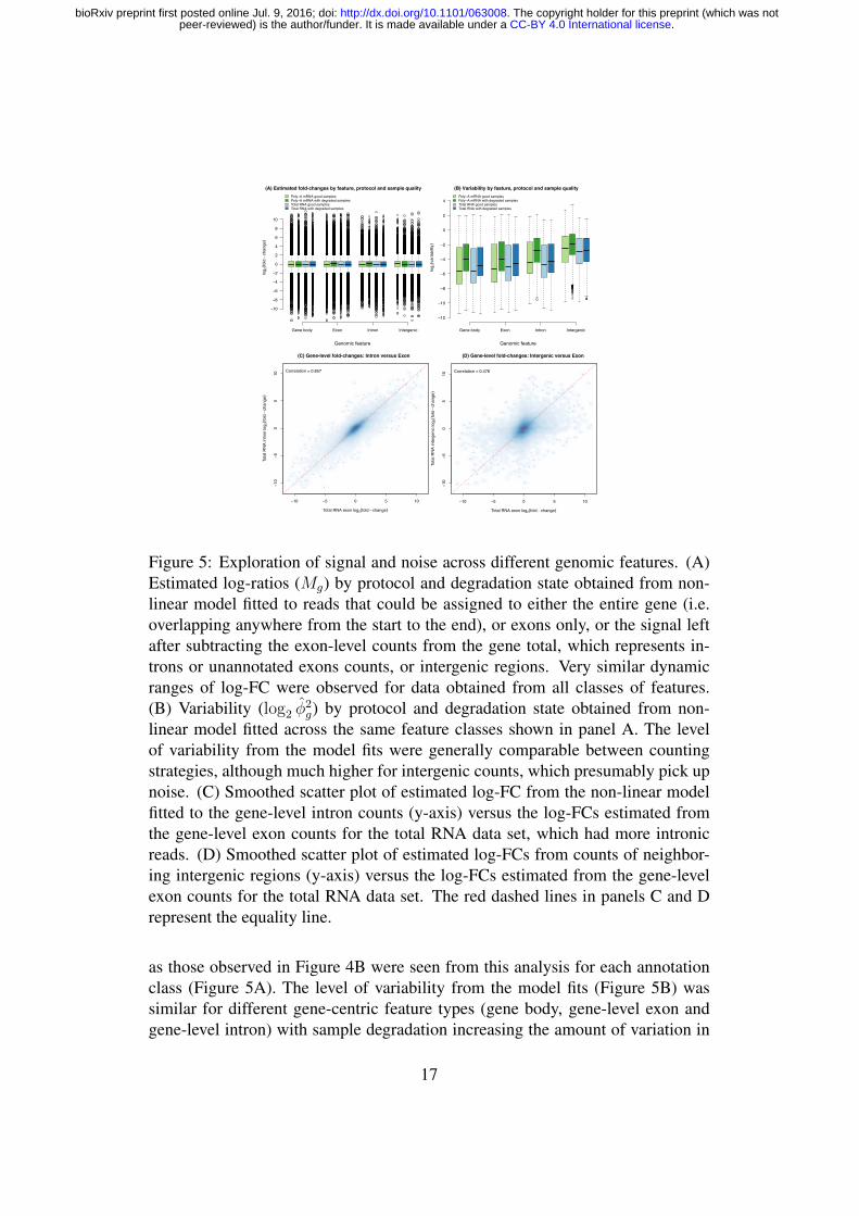
(A) Estimated fold-changes by feature, protocol and sample quality (B) Variability by feature, protocol and sample quality

(C) Gene-level fold-changes: Intron versus Exon

log 2

(fold

−ch

ange

)

Gene body Exon Intron Intergenic

−10

−8

−6

−4

−2

0

2

4

6

8

10

Poly−A mRNA good samplesPoly−A mRNA with degraded samplesTotal RNA good samplesTotal RNA with degraded samples

log 2

(var

iabi

lity)

Gene body Exon Intron Intergenic

−12

−10

−8

−6

−4

−2

0

2

4Poly−A mRNA good samplesPoly−A mRNA with degraded samplesTotal RNA good samplesTotal RNA with degraded samples

Genomic feature Genomic feature

−10 −5 0 5 10

−10

−50

510

Total RNA exon log2(fold − change)

Tota

l RN

A in

tron

log 2

(fold

−ch

ange

)

Correlation = 0.857

(D) Gene-level fold-changes: Intergenic versus Exon

−10 −5 0 5 10

−10

−50

510

Total RNA exon log2(fold − change)

Tota

l RN

A in

terg

enic

log 2

(fold

−ch

ange

)

Correlation = 0.476

Figure 5: Exploration of signal and noise across different genomic features. (A)Estimated log-ratios (Mg) by protocol and degradation state obtained from non-linear model fitted to reads that could be assigned to either the entire gene (i.e.overlapping anywhere from the start to the end), or exons only, or the signal leftafter subtracting the exon-level counts from the gene total, which represents in-trons or unannotated exons counts, or intergenic regions. Very similar dynamicranges of log-FC were observed for data obtained from all classes of features.(B) Variability (log2 φ2

g) by protocol and degradation state obtained from non-linear model fitted across the same feature classes shown in panel A. The levelof variability from the model fits were generally comparable between countingstrategies, although much higher for intergenic counts, which presumably pick upnoise. (C) Smoothed scatter plot of estimated log-FC from the non-linear modelfitted to the gene-level intron counts (y-axis) versus the log-FCs estimated fromthe gene-level exon counts for the total RNA data set, which had more intronicreads. (D) Smoothed scatter plot of estimated log-FCs from counts of neighbor-ing intergenic regions (y-axis) versus the log-FCs estimated from the gene-levelexon counts for the total RNA data set. The red dashed lines in panels C and Drepresent the equality line.

as those observed in Figure 4B were seen from this analysis for each annotationclass (Figure 5A). The level of variability from the model fits (Figure 5B) wassimilar for different gene-centric feature types (gene body, gene-level exon andgene-level intron) with sample degradation increasing the amount of variation in

17

.CC-BY 4.0 International licensepeer-reviewed) is the author/funder. It is made available under aThe copyright holder for this preprint (which was not. http://dx.doi.org/10.1101/063008doi: bioRxiv preprint first posted online Jul. 9, 2016;

all cases. Interestingly, results from the gene body counting approach are slightlyless variable on average than the exon-only results. Results for intergenic regionsprovide the negative control here, with systematically higher variation than theother feature types. Figure 5C shows a smoothed scatter plot of estimated log-ratios from the non-linear model fitted to the gene-level intron counts (y-axis)versus the log-ratios estimated from the gene-level exon counts (x-axis) for thesame gene for the total RNA data set, which had more intronic reads (Figure 2A).The log-ratios showed good agreement, with a Pearson correlation of 0.86. A sim-ilar plot displaying the log-ratios obtained from intergenic regions neighbouringa given gene versus the log-ratios from gene-level exon counts has much lowercorrelation of 0.48 (Figure 5D). While exonic reads are mainly contributed by themore abundant mature mRNAs, intronic signal at the gene-level can presumablybe attributed to pre-messenger RNA (pre-mRNA). Since these pre-mRNAs arelikely to have a similar relative concentration to their mature counterparts, includ-ing these intron reads in the gene-level counts is therefore likely to boost signal,rather than add noise, increasing power.

Differential expression: 7 methods comparedDifferential expression analysis was carried out using 7 popular methods availableas part of the Bioconductor project [30]: edgeR [31] using the method of exacttests (edgeR-classic) [32] or with generalized linearized models and likelihoodratio tests (edgeR-glm) [33]; baySeq [34, 35] with counts modelled either by neg-ative binomial distributions (baySeq) or by normal distributions (baySeq-norm);limma-voom [36, 21] either with default settings (voom) or with sample qualityweights (voom-qw) [37]; and DESeq2 [38]. Although all of the above softwarepackages are able to analyze more than two experimental conditions in one anal-ysis, the results we present here are for simple two group comparisons betweendifferent mixing proportions. This mimics what is perhaps the most commonreplicated RNA-seq experimental design in practice, a two group comparison with3 replicate RNA samples in each group (6 samples in total).

A characteristic of the mixture design is that the same set of genes must be DEbetween any pair of samples. If a gene is DE between the two pure reference sam-ples, then it should also be DE between any pair of samples with different mixingproportions. However the FCs will be largest when comparing pure samples andcorrespondingly smaller when comparing intermediate mixtures. Unsupervisedclustering of samples confirms that the pure samples have the most extreme tran-scriptional profiles (Figure 2C-D). It follows that the two group comparison ofthe pure samples (100vs000) should result in the greatest number of statisticallysignificant DE genes, at any given false discovery rate (FDR). Any two groupcomparison between other good samples, such as 75 and 25 (075vs025), 50 and

18

.CC-BY 4.0 International licensepeer-reviewed) is the author/funder. It is made available under aThe copyright holder for this preprint (which was not. http://dx.doi.org/10.1101/063008doi: bioRxiv preprint first posted online Jul. 9, 2016;

34

85

763

25

132

10,084

240

3599

164 103 19 21

7

5

baySeq−norm DESeq2

edgeR−glm voom−qwR

ecov

ery

rate

100v

s000

075v

s025

050v

s025

075v

s050

0%

25%

50%

75%

100%

100v

s000

d

075v

s025

d

050v

s025

d

075v

s050

d

baySeqbaySeq−normDESeq2edgeR−classicedgeR−glmvoom−qwvoom

(A) Good samples only (B) Good and degraded samples (C) DE genes in 100vs000

0%

25%

50%

75%

100%

Figure 6: Recovery rate of differential expression methods. The rate at which DEgenes are recovered from 100vs000 are displayed for comparisons using goodsamples only (A) and for those using good and degraded samples (B). Eachmethod is shown in a distinct colour, with different line-types used when resultsare overlapping to allow them to be distinguished from one and other. The num-ber of common DE genes for 100vs000 across select methods are displayed in (C).For a given software package, only the method with higher recovery is shown.

25 (050vs025), or 75 and 50 (075vs050), should ideally result in significant genesthat are a subset of those observed in the 100vs000 comparison.

The mixture experiment has no true positives or true negatives for differentialexpression that are known a priori. However we can compare methods by wayof their sensitivity, recovery and inconsistency rates. ‘Sensitivity’ can be mea-sured by the total number of DE genes detected. Supplementary Figure 4 showsthe number of discoveries made (at a FDR < 0.05 cutoff), which gradually de-creases for all 7 methods as the RNA samples compared become more similar inconcentration. Using the 075vs025 comparison as an example, ‘recovery’ refersto the proportion of DE genes detected in 100vs000 that are also detected as DEin 075vs025 by the same method, while ‘inconsistency’ refers to the proportionof DE genes in 075vs025 that are not detected in 100vs000 by the same method.Analogous recovery and inconsistency rates can be computed for the 050vs025and 075vs050 comparisons. These measures examine the performance of eachmethod in the presence of small transcriptional differences, and more specifically,assess how much the power of each method is affected by systematically reducingexpression differences. At the same time, we consider the rate of inconsistency tobe a reflection of the ‘error’ of a method.

Using a 5% FDR cutoff, voom-qw is not only the most sensitive method, but italso achieves the highest recovery rate across all comparisons between good sam-ples (Figure 6A and Supplementary Table 2). For moderate differences in propor-tions (075vs025), voom-qw achieves 82% recovery of DE genes from 100vs000and 37-39% recovery for subtle differences (050vs025 and 075vs050). Thus

19

.CC-BY 4.0 International licensepeer-reviewed) is the author/funder. It is made available under aThe copyright holder for this preprint (which was not. http://dx.doi.org/10.1101/063008doi: bioRxiv preprint first posted online Jul. 9, 2016;

voom-qw retains much of its power even when transcriptional differences are re-duced. Most other methods have recovery rates only moderately lower than that ofvoom-qw, except for baySeq and baySeq-norm which have much lower recoveryrates than the other methods: 62–65% for 075vs050, and 10–14% for 050vs025and 075vs050. baySeq loses power more quickly than the other methods when thetranscriptional differences are small.

The experimental design allows us to perform an analysis on the regular sam-ples and compare our results to the analysis that includes the degraded samples.Replacing the non-degraded replicate 2 with the degraded sample results in extrawithin-group variability that can be observed in the vertical spread of points in theMDS plot in Figure 2C for the poly-A mRNA data. Comparisons with degradedsamples will be referred to as 100vs000d, 075vs025d, 050vs025d and 075vs050drespectively. These degraded samples are intended to represent low quality sam-ples that are frequently observed in practice [39].

As expected, increasing within-group variability results in lower recovery ratesfor all methods. In particular, the recovery rates are 68–82% for 100vs000d ascompared to 100vs000 (Figure 6B). The voom-qw method has the highest re-covery rate for 100vs000d and 075vs025d while DESeq2 has highest recoveryby a narrow margin for the most subtle comparisons 050vs025d and 075vs050d.The two baySeq methods again have the lowest recovery rates, with the negativebinomial modelling of baySeq the lowest out of the 7 methods compared. Allmethods detect differential expression consistently, with low inconsistency ratesobserved across all comparisons with or without degraded samples (Supplemen-tary Table 2). For large to moderate proportion differences (100vs000d, 075vs025and 075vs025d) inconsistency rates sit at between 0-1.7%. For subtle proportiondifferences (050vs025, 050vs025d, 075vs050 and 075vs050d) inconsistency is be-tween 0-0.3%. Although recovery and inconsistency is assessed for each methodrelative to itself, it is worth noting that most genes detected as DE in the 100vs000comparison are common to all methods, with an overlap of 10,084 genes (Figure6C). The voom-qw method detects the most unique DE genes (763) and DESeq2detects the least unique DE genes (7).

In addition to within-method comparisons, bias can be examined by lookingat differences between the log-FC estimated by each method and those predictedby the non-linear model (Mg) over the entire data set and adjusted according tothe relevant sample concentrations for the two-group comparisons (see Methods,Equation 2). Predicted log-FCs are calculated using information from all goodsamples across the experiment – a total of 15 samples. On the other hand, the log-FCs estimated by each differential expression method are based only on the 6 sam-ples included in that particular analysis. For this reason, we assume that predictedlog-FCs are more accurate than the estimated log-FCs. baySeq and baySeq-normdo not estimate gene-wise log-FCs, so were not included in this comparison.

20

.CC-BY 4.0 International licensepeer-reviewed) is the author/funder. It is made available under aThe copyright holder for this preprint (which was not. http://dx.doi.org/10.1101/063008doi: bioRxiv preprint first posted online Jul. 9, 2016;

−10 −5 0 5 10

−10

−5

0

5

10

SD=0.211

−10 −5 0 5 10

−10

−5

0

5

10

SD=0.185

−10 −5 0 5 10

−10

−5

0

5

10

SD=0.129

−10 −5 0 5 10

−10

−5

0

5

10

SD=0.05

−10 −5 0 5 10

−10

−5

0

5

10

SD=0.219

−10 −5 0 5 10

−10

−5

0

5

10

SD=0.226

−10 −5 0 5 10

−10

−5

0

5

10

SD=0.141

−10 −5 0 5 10

−10

−5

0

5

10

SD=0.139

−1.0

−0.5 0.0

0.5

1.0

−1.0

−0.5

0.0

0.5

1.0

SD=0.108

−1.0

−0.5 0.0

0.5

1.0

−1.0

−0.5

0.0

0.5

1.0

SD=0.085

−1.0

−0.5 0.0

0.5

1.0

−1.0

−0.5

0.0

0.5

1.0

SD=0.09

−1.0

−0.5 0.0

0.5

1.0

−1.0

−0.5

0.0

0.5

1.0

SD=0.087

−1.0

−0.5 0.0

0.5

1.0

−1.0

−0.5

0.0

0.5

1.0

SD=0.122

−1.0

−0.5 0.0

0.5

1.0

−1.0

−0.5

0.0

0.5

1.0

SD=0.093

−1.0

−0.5 0.0

0.5

1.0

−1.0

−0.5

0.0

0.5

1.0

SD=0.107

−1.0

−0.5 0.0

0.5

1.0

−1.0

−0.5

0.0

0.5

1.0

SD=0.095

DESeq2 edgeR-glm voom-qw voom

100v

s000

d10

0vs0

00

Pred

icte

d lo

g-FC

Pred

icte

d lo

g-FC

075v

s050

d07

5vs0

50

Pred

icte

d lo

g-FC

Pred

icte

d lo

g-FC

Estimated log-FC Estimated log-FC Estimated log-FC Estimated log-FC

Figure 7: Accuracy of log-FCs estimated by differential expression methods.Gene-wise log-FCs estimated by methods are plotted against predicted log-FCs.Areas with high density of points are shaded in blue, where colour intensity re-flects the density of points. Red lines mark equality between estimated and pre-dicted log-FCs. Standard deviations (SD) between estimated and predicted log-FCs are displayed in each panel.

Estimates from voom match closest to predicted log-FCs for 100vs000 and100vs000d, with a strikingly near-perfect match when only good samples are used(Figure 7). The tail-end of log-FCs suggests that DESeq2 is slightly conservative,where the magnitude of estimated log-FCs tends to be slightly smaller than thepredicted values; whilst edgeR is slightly liberal, with estimated values slightlylarger than predicted values. edgeR-glm and edgeR-classic produce almost identi-cal log-FC estimates. The concordance between estimated and predicted log-FCsdrops in 075vs050 and 075vs050d, when the differences are most subtle. Here,edgeR-glm estimates log-FCs marginally better than voom, matching closest tothe predicted values. Across all comparisons, DESeq2 estimates are most biased,with the greatest deviation from the predicted values.

21

.CC-BY 4.0 International licensepeer-reviewed) is the author/funder. It is made available under aThe copyright holder for this preprint (which was not. http://dx.doi.org/10.1101/063008doi: bioRxiv preprint first posted online Jul. 9, 2016;

Comparing variability levels between our mixture and SEQCAnother issue to consider is whether these data sets contain more variability thancomparable control data sets that are dominated by technical variation. To as-sess this, we looked at the prior degrees of freedom obtained from the edgeR-glmanalysis fitted to all good samples only or the good and degraded samples (15samples in each analysis). The pilot SEQC RNA-seq data set from Law et al.(2014) [21] which consisted of 16 samples (4 samples for A, B, C, and D) wasalso analysed using edgeR-glm. The SEQC data set was pre-processed by filter-ing genes with low counts (CPM > 1 in at least 4 samples was required), thenTMM normalized. The prior degrees of freedom was estimated to be 5.30 usingthe good samples, 4.53 for the good and degraded samples and 67.7 for the SEQCdata set. This value measures the consistency of the gene-wise dispersions, with asmaller prior degrees of freedom indicating the values are more gene-specific (i.e.there is more biological variation) and larger values indicating that they are moreconsistent (i.e. there is more technical variation) and will be more heavily shrunkto a common value. Repeating this analysis with limma voom gave similar resultswith prior degrees of freedom values estimated as 5.29, 4.54 and 45.3 respectivelyfor the 3 data sets. Plotting the biological coefficient of variation (BCV) from theedgeR-glm analysis offers another way to visualise this (Supplementary Figure5). Much greater spread in gene-level variability is observed in the current mix-ture experiment (Supplementary Figure 5A and 5B) compared to the SEQC dataset (Supplementary Figure 5C) in which all genes at a particular expression levelhave a very similar BCV. This analysis shows that our efforts to simulate addi-tional noise over and above pure technical noise were successful, with our datasets having systematically higher variability than the pilot SEQC data set.

Differential splicing: 3 methods comparedDetection of differentially spliced (DS) genes was carried out using 3 availableBioconductor methods for the analysis of exon counts: DEXSeq [40], edgeR-ds[33], and voom-ds [36] (see Methods). The recovery rate and inconsistency rate ofeach method is examined as it was for differential expression. Rate of recovery isdefined as the proportion of DS genes detected in 100vs000 that are also detectedin another comparison (075vs025, 050vs025 or 075vs050) by the same method.The rate of inconsistency is defined as the proportion of genes detected as DS in aparticular comparison (075vs025, 050vs025 or 075vs050) that were not detectedin the 100vs000 comparison by the same method.

Using only the good samples, the recovery rates of the 3 methods were similarfor each comparison, with DEXSeq having slightly higher recovery than edgeR-ds or voom-ds (Figure 8A). Compared to the differential expression analysis, the

22

.CC-BY 4.0 International licensepeer-reviewed) is the author/funder. It is made available under aThe copyright holder for this preprint (which was not. http://dx.doi.org/10.1101/063008doi: bioRxiv preprint first posted online Jul. 9, 2016;

612 3 13

96448

8

19

DEXSeq voom−ds

edgeR−ds

Rec

over

y ra

te

100v

s000

075v

s025

050v

s025

075v

s050

0%

25%

50%

75%

100% DEXSeqvoom−dsedgeR−ds

Inco

nsis

tenc

y ra

te

100v

s000

075v

s025

050v

s025

075v

s050

0%

10%

20%

30%

40%(A) Good samples only (B) Good samples only (C) DS genes in 100vs000

Figure 8: Recovery and inconsistency rate of differential splicing methods. Therate at which DS genes are recovered from 100vs000 (A) and the inconsistencyof detected genes (B) are displayed for comparisons using good samples only.Each method is shown in a distinct colour, line-type combination. The number ofcommon DS genes for 100vs000 across the three methods are displayed in panelC.

differential splicing methods rapidly lose the ability to recover DS genes from the100vs000 comparison when the samples become more similar – 33-41% recoveryfor 075vs025, and 2-7% recovery for 050vs025 and 075vs050.

Although DEXSeq achieves slightly better recovery than edgeR-ds and voom-ds, this advantage is negated by its very high inconsistency rate (Figure 8B). Forthe comparisons between subtle proportion differences, methods are expected tohave both low recovery and inconsistency rates since methods should be conser-vative in theory. For comparisons of mixed samples, 33-40% of the genes de-tected as DS by DEXSeq are not detected in its corresponding 100vs000 analysis.This means that a third or more of these DS genes did not achieve significancein the comparison between the pure samples where DS genes can be detectedconfidently, but were significant when the between sample differences were moresubtle.

On the other hand, voom-ds and edgeR-ds achieve much lower rates of incon-sistency, with voom-ds being the least inconsistent. For 075vs025, voom-ds andedgeR-ds have inconsistency rates of 8% and 10% respectively. These rates fallto 0% in voom-ds, and 0-6% in edgeR-ds, for the 050vs025 and 075vs050 com-parisons which are the most subtle. Both of these methods have comparable, butslightly lower recovery rates than DEXSeq, however, any gene that is detected asDS by these two methods are likely to be also detected in the 100vs000 compari-son. This may suggest that voom-ds and edgeR-ds have low FDRs.

Overall, DEXSeq appears to be liberal relative to voom-ds and edgeR-ds. For100vs000, 448 genes are commonly detected by all three methods (37% of the

23

.CC-BY 4.0 International licensepeer-reviewed) is the author/funder. It is made available under aThe copyright holder for this preprint (which was not. http://dx.doi.org/10.1101/063008doi: bioRxiv preprint first posted online Jul. 9, 2016;

total DS genes identified by any method, Figure 8C), which is much lower thanwas observed for the differential expression analysis (85%, Figure 6C). Another612 genes are detected only by DEXSeq whereas voom-ds and edgeR-ds uniquelydetect 13 and 19 DS genes, respectively (Figure 8C).

Results from comparisons between the mixture samples (075vs025, 050vs025and 075vs050) indicate that the differential splicing methods deteriorate morerapidly than the differential expression analysis methods when the expressionchanges become more subtle, with lower recovery rates and higher inconsistencyrates. In general, differential splicing analysis is more complex and challeng-ing than differential expression analysis. Detection of differential exon usage isequivalent to a statistical test of interaction rather than of a simple change in levelbetween two treatment conditions, so there is less statistical power to detect differ-ential splicing. Furthermore, the total gene-level read counts used for differentialexpression analysis are spread over several exons per gene, leaving much lowercounts per feature for exon-level analysis.

Deconvolution analysis: DeMix versus ISOpureThe mixture design is also ideal for comparing methods that aim to determinethe proportions of different sample types present in heterogeneous samples. Tothis end, we estimate mixture proportions for 12 poly-A mRNA samples using thestatistical methods DeMix [24] and ISOpure [25]. These methods determine theproportions of two different cell populations (typically normal and cancer cellsin a patient sample) present in a mixed sample and deconvolve the expressionprofiles. The input matrix for both methods are read counts from the four puresamples of each type (100, 0) and the twelve mixed samples (4 each of 75, 50 and25). After filtering based on FC cutoffs of >1.5 or <0.667, only 2,055 informa-tive genes remained. As shown in Table 1, DeMix yielded proportion estimatesthat were closer to the ground truth (differences of less than 10%) while ISOpurelargely overestimated mixture proportions across all 12 samples. We also com-pared the deconvolved expression values from the two methods with the four puresamples using Pearson correlation coefficients. The correlations from DeMix areall above 0.95 and were generally higher than those obtained from ISOpure (Table1). This analysis clearly demonstrates that DeMix is a more reliable method fordeconvolution analysis.

DISCUSSIONFor common tasks like differential expression analysis, there have been manycomparison studies that have arrived at different conclusions on the ‘best’ method

24

.CC-BY 4.0 International licensepeer-reviewed) is the author/funder. It is made available under aThe copyright holder for this preprint (which was not. http://dx.doi.org/10.1101/063008doi: bioRxiv preprint first posted online Jul. 9, 2016;

Table 1: (Top) Mixture proportions estimated from each sample from the plotAmRNA data by the reference free methods DeMix and ISOpure. The results forthe degraded sample is listed last in each cell in italics and the values closest tothe true values are underlined. In each case, DeMix recovers values closest to thetrue values shown in the bottom row. Pearson correlation coefficients calculatedbetween each of the deconvolved expression profiles mixed samples and the asso-ciated pure tumor sample are also shown. The highest correlation coefficients foreach sample is again underlined. Of the two methods compared, DeMix tends tohave higher correlations (closer to 1).

Method 25:75 50:50 75:25DeMix (estimated proportion) 0.311,0.294,0.284,0.247 0.563,0.544,0.518,0.516 0.759,0.730,0.751,0.733

DeMix (correlation) 0.994,0.986,0.989,0.996 0.987,0.986,0.959,0.956 0.964,0.998,0.998,0.964ISOpure (estimated proportion) 0.654,0.673,0.655,0.615 0.917,0.913,0.908,0.883 1.00,1.00,1.00,1.00

ISOpure (correlation) 0.975,0.971,0.976,0.965 0.973,0.968,0.946,0.955 0.959, 0.986, 0.987, 0.964True proportion 0.25 0.5 0.75

using different data sets (both simulated and experimental) and assessment criteria[41, 42, 21, 38, 43, 44, 45, 46]. Some find voom to be best [21, 41], or edgeR [42,45], or DESeq2 [38, 44] or edgeR and DESeq2 to be equal best [43]. In terms ofour main results from comparing DE testing methods on our mixture data set, wefind voom-qw to be most sensitive followed by DESeq2, edgeR (glm and classic),voom and finally baySeq (both normal and regular) is the least sensitive. Recentwork has shown that combining differential expression methods in a weightedmanner [47] can offer better results than relying on individual methods. Furtherexploration of this approach on data sets such as this, while including methodssuch as voom-qw would be an interesting topic for future research. Optimisingsuch an approach has the potential to ensure, that for any given data set, the bestpossible results are obtained.

For differential splicing, our study is the first to compare DEXSeq with thecompeting methods in edgeR and limma. The latter methods were found to bemore conservative than DEXSeq, identifying somewhat fewer differential splicingevents, but achieved much better consistency than DEXSeq, which seems to havea high empirical false positive rate.

Unlike the study of Gallego Romero et al. (2014) [48], who degrade PBMCsamples by leaving them at room temperature for varying lengths of time, ourwork couples sample degradation with a classic mixture design, which allowsprecision and bias to be assessed for every expressed gene. Our experiment has3 replicate samples per mixture, which is close to the minimum that can be usedfor tasks like differential expression analysis and differential splicing analysis, soour comparisons should be interpreted with this in mind, in that we are workingin the most difficult setting, which is nonetheless a common one in practice. A

25

.CC-BY 4.0 International licensepeer-reviewed) is the author/funder. It is made available under aThe copyright holder for this preprint (which was not. http://dx.doi.org/10.1101/063008doi: bioRxiv preprint first posted online Jul. 9, 2016;

limitation of the current study is that we simulated a third of the data to be morevariable by degrading one sample from each of pure and mixed group. This studydesign particularly tests the ability of differential expression methods to tolerateheterogeneous variability across the samples. If we turn this around and havethe majority of samples being more variable, tasks like detecting differential ex-pression with such a small sample size will become much harder and yield manyfewer significant results, irrespective of the method chosen, particularly for themore subtle mixture comparisons.

Further extensions to this experiment could include other library preparationmethods, such as exome capture, which has been shown to improve the resultsfrom degraded samples [49] or Globin depletion methods [50], although the mix-ture would need to re-designed to include an appropriate blood sample to makethis comparison informative. The inclusion of controls such as the External RNAControls Consortium (ERCC) spike-in mixes (1 and 2) in different samples isanother enhancement that would provide transcripts with known FCs as a fur-ther tool for assessing bias. Other genomics applications, such as ChIP-seq orRNA-seq using new technologies, such as long read sequencing platforms fromcompanies such as Pacific Biosciences (Sequel) or Oxford Nanopore Technology(MinION and PromethION) could also benefit from having available a referencedata set such as this to allow methodology testing and inter-platform comparisons.

Our analysis has included many of the most popular Bioconductor tools but isnot intended as an exhaustive methods comparison. Different algorithms for othercommon analysis tasks such as read alignment and gene counting, normalization,fusion-detection, intron retention analysis and gene set testing, to name a few pos-sibilities, could also be compared using this data set. We also did not test everycapability of the software packages, in particular, we have not tested the abilityof the software packages to analyse complex experimental designs with multipletreatment factors and blocking variables. We have also not tested the newer fea-tures of some of the packages, for example edgeR’s robust dispersion estimation[51], edgeR’s quasi-likelihood pipeline [52] or limma’s robust empirical Bayes[53]. A natural way to facilitate widespread systematic evaluations of other meth-ods would be to incorporate this data set into one of the recently released RNA-seqbenchmarking tools such as RNASEQcomp [54] or RNAonthebench [55].

CONCLUSIONWe have generated a unique control experiment that is the first to include sample-level heterogeneity induced by systematically degrading samples in order to simu-late this routine source of variation. The variability added to our study has shiftedthe noise profile away from the pure technical end of the spectrum typical of

26

.CC-BY 4.0 International licensepeer-reviewed) is the author/funder. It is made available under aThe copyright holder for this preprint (which was not. http://dx.doi.org/10.1101/063008doi: bioRxiv preprint first posted online Jul. 9, 2016;

previous mixture experiments much closer to variation levels seen in regular ex-periments. The classic mixture design allows precision and bias to be quantifiedvia a non-linear model for each gene, and used as a basis for comparing differentsample preparation methods. The comparison of poly-A mRNA and total RNAsample preparation kits from Illumina saw differences in the detection of severalRNA classes, with more reads mapping to ncRNA, snoRNAs and snRNAs us-ing the total RNA protocol. This comes at a price, with the total RNA protocolsequencing a greater number of intronic reads compared to the poly-A method.Our investigations showed that these intronic reads measure signal rather thanrandom noise irrespective of the library preparation method used. The estimatedlog-FCs obtained from modelling either intron counts or exon counts at the gene-level were highly correlated, indicating that including these reads in gene-levelanalyses rather than ignoring them as is standard practice offers a simple way toboost signal on the order of 20-30%. This observation warrants further investi-gation using other published RNA-seq data through re-analysis with and withoutthe intronic reads. It could deliver savings on the cost of sequencing by allowingmore samples to be multiplexed per run for an equivalent amount of gene-centricsequencing once exon and intron reads are pooled. The inclusion of degradedsamples in the analysis had a more profound effect on the variability of the poly-A mRNA data than the total RNA data, which suggests that the latter method isthe best choice in experiments where degraded samples are expected, such as inclinical studies.

This mixture design also allows for internal comparisons to be made withinmethods for benchmarking differential expression and differential splicing analy-sis methods. How well a given method can detect changes when the differencesare large and relatively easy to detect is used as the ‘true positive’ set and com-pared to the results obtained when an independent set of samples which showmore subtle changes are compared in a pair-wise manner.

Although most methods perform well at recovering these ‘true positives’ withhigh overlap in the easiest ’pure versus pure’ comparison (100vs000), the voom-qw method which explicitly deals with sample-level variation slightly outperformsother methods, with DESeq2 second best, followed by the two edgeR methodswhich perform similarly, then standard voom, and finally the two baySeq methodswhich have the least power and consistency.

In terms of bias, DESeq2 gives FCs that underestimate the consensus valuesobtained from the non-linear model, indicating that its shrinkage procedure givesconservative results. For differential splicing methods, edgeR-ds and voom-dswere found to both be conservative relative to the most popular method, DEXSeq,however DEXSeq tended to have a high empirical false positive rate compared tothese other methods based on the within method inconsistency rate.

This is the first time that a mixture experiment has been used to benchmark

27

.CC-BY 4.0 International licensepeer-reviewed) is the author/funder. It is made available under aThe copyright holder for this preprint (which was not. http://dx.doi.org/10.1101/063008doi: bioRxiv preprint first posted online Jul. 9, 2016;

methods for this application. The results from the deconvolution analysis showedthat DeMix consistently outperformed ISOpure. Our work demonstrates the utilityof carefully designed control experiments for benchmarking library preparationkits and analysis methods.

FUNDINGThis work was supported by the National Health and Medical Research Council(Project grants 1050661 (MER, GKS, MLAL), 1079756 (MLAL, MER), 1045936(MER) and 1059622 (MER); Fellowships 1104924 (MER) and 1058892 (GKS)),Victorian State Government Operational Infrastructure Support, Australian Gov-ernment NHMRC IRIISS and the Ian Potter Centre for Genomics and Person-alised Medicine.

ACKNOWLEDGEMENTSWe thank Dr Yunshun Chen and Dr Wei Shi for analysis advice and Dr StephenWilcox for technical advice on RNA-seq protocols.

AUTHOR’S CONTRIBUTIONSAZH performed the experiments. AZH, CWL, RL, ZW, WW, JA and MER per-formed analysis. AZH, MLAL, GKS and MER designed research. AZH, CWL,WW, JA, GKS and MER wrote the manuscript with the help of the other co-authors.

Conflict of interest statement.

None declared.

References[1] Lockhart,D.J., Dong,H., Byrne,M.C., Follettie,M.T., Gallo,M.V.,

Chee,M.S., Mittmann,M., Wang,C., Kobayashi,M., Horton,H. et al. (1996)Expression monitoring by hybridization to high-density oligonucleotidearrays. Nat Biotechnol, 14, 1675–80.

28

.CC-BY 4.0 International licensepeer-reviewed) is the author/funder. It is made available under aThe copyright holder for this preprint (which was not. http://dx.doi.org/10.1101/063008doi: bioRxiv preprint first posted online Jul. 9, 2016;

[2] Cope,L.M., Irizarry,R.A., Jaffee,H.A., Wu,Z. and Speed,T.P. (2004) Abenchmark for Affymetrix GeneChip expression measures. Bioinformatics,20, 323–331.

[3] Irizarry,R.A., Wu,Z. and Jaffee,H.A. (2006) Comparison of AffymetrixGeneChip expression measures. Bioinformatics, 22, 789–794.

[4] Wu,Z. (2009) A Review of Statistical Methods for Preprocessing Oligonu-cleotide Microarrays. Stat Methods Med Res, 18, 533–41.

[5] Lemon,W., Palatini,J., Krahe,R. and Wright,F. (2002) Theoretical and em-pirical comparisons of gene expression indexes for oligonucleotide arrays.Bioinformatics, 18, 1470–76.

[6] He,Y.D., Dai,H., Schadt,E.E., Cavet,G., Edwards,S.W., Stepaniants,S.B.,Duenwald,S., Kleinhanz,R., Jones,A.R., Shoemaker,D.D. et al. (2003) Mi-croarray standard data set and figures of merit for comparing data processingmethods and experiment designs. Bioinformatics, 19, 956–65.

[7] Barnes,M., Freudenberg,J., Thompson,S., Aronow,B. and Pavlidis,P. (2005)Experimental comparison and cross-validation of the Affymetrix and Illu-mina gene expression analysis platforms. Nucleic Acids Res, 33, 5914–23.

[8] Holloway,A.J., Oshlack,A., Diyagama,D.S., Bowtell,D.D. and Smyth,G.K.(2006) Statistical analysis of an RNA titration series evaluates microarrayprecision and sensitivity on a whole-array basis. BMC Bioinformatics, 7,511.

[9] MAQC Consortium (2006) The MicroArray Quality Control (MAQC)project shows inter- and intraplatform reproducibility of gene expressionmeasurements. Nat Biotechnol, 24, 1151–1161.

[10] SEQC/MAQC-III Consortium (2014) A comprehensive assessment of RNA-seq accuracy, reproducibility and information content by the SequencingQuality Control Consortium. Nat Biotechnol, 32, 903–14.

[11] Zakharkin,S.O., Kim,K., Mehta,T., Chen,L., Barnes,S., Scheirer,K.E.,Parrish,R.S., Allison,D.B. and Page,G.P. (2005) Sources of variation inAffymetrix microarray experiments. BMC Bioinformatics, 6, 214.

[12] Boedigheimer,M.J., Wolfinger,R.D., Bass,M.B., Bushel,P.R., Chou,J.W.,Cooper,M., Corton,J.C., Fostel,J., Hester,S., Lee,J.S. et al. (2008) Sourcesof variation in baseline gene expression levels from toxicogenomics studycontrol animals across multiple laboratories. BMC Genomics, 9, 285.

29

.CC-BY 4.0 International licensepeer-reviewed) is the author/funder. It is made available under aThe copyright holder for this preprint (which was not. http://dx.doi.org/10.1101/063008doi: bioRxiv preprint first posted online Jul. 9, 2016;

[13] Hansen,K.D., Wu,Z., Irizarry,R.A. and Leek,J.T. (2011) Sequencing tech-nology does not eliminate biological variability. Nature Biotech, 29, 572–3.

[14] Liao,Y., Smyth,G.K. and Shi,W. (2013) The Subread aligner: fast, accurateand scalable read mapping by seed-and-vote. Nucleic Acids Res, 41, e108.

[15] Liao,Y., Smyth,G.K. and Shi,W. (2014) featureCounts: an efficient general-purpose program for assigning sequence reads to genomic features. Bioin-formatics, 30, 923–30.

[16] Wang,L., Wang,S. and Li,W. (2012) RSeQC: Quality Control of RNA-seqexperiments. Bioinformatics, 28, 2184–5.

[17] Smyth,G. (1996) Partitioned algorithms for maximum likelihood and othernon-linear estimation. Statistics and Computing, 6, 201–216.

[18] Bullard,J.H., Purdom,E., Hansen,K.D. and Dudoit,S. (2010) Evaluation ofstatistical methods for normalization and differential expression in mRNA-Seq experiments. BMC Bioinformatics, 11, 94.

[19] Anders,S. and Huber,W. (2010) Differential expression analysis for sequencecount data. Genome Biology, 11, R106.

[20] Robinson,M.D. and Oshlack,A. (2010) A scaling normalization method fordifferential expression analysis of RNA-seq data. Genome Biology, 11, R25.

[21] Law,C.W., Chen,Y., Shi,W. and Smyth,G.K. (2014) Voom: precision weightsunlock linear model analysis tools for RNA-seq read counts. Genome Biol-ogy, 15, R29.

[22] Chen,Y., Lun,A. and Smyth,G. (2014) Differential expression analysis ofcomplex RNA-seq experiments using edgeR. In Datta,S. and Nettleton,D.S.(eds.), Statistical Analysis of Next Generation Sequence Data, Springer, NewYork, pp. 51–74.

[23] Benjamini,Y. and Hochberg,Y. (1995) Controlling the false discovery rate:a practical and powerful approach to multiple testing. Journal of the RoyalStatistical Society: Series B, 57, 289–300.

[24] Ahn,J., Yuan,Y., Parmigiani,G., Suraokar,M.B., Diao,L., Wistuba,I.I. andW,W. (2013) DeMix: deconvolution for mixed cancer transcriptomes usingraw measured data. Bioinformatics, 29, 1865–71.

30

.CC-BY 4.0 International licensepeer-reviewed) is the author/funder. It is made available under aThe copyright holder for this preprint (which was not. http://dx.doi.org/10.1101/063008doi: bioRxiv preprint first posted online Jul. 9, 2016;

[25] Quon,G., Haider,S., Deshwar,A.G., Cui,A., Boutros,P.C. and Morris,Q.D.(2013) Computational purification of individual tumor gene expression pro-files leads to significant improvements in prognostic prediction. GenomeMedicine, 5, 29.

[26] Shen-Orr,S.S. and Gaujoux,R. (2013) Computational deconvolution: ex-tracting cell type-specific information from heterogeneous samples. CurrentOpinion in Immunology, 25, 571–8.

[27] R Development Core Team (2016) R: A language and environment for sta-tistical computing. R Foundation for Statistical Computing, Vienna.

[28] Zhao,W., He,X., Hoadley,K.A., Parker,J.S., Hayes,D.N. and Perou,C.M.(2014) Comparison of RNA-Seq by poly (A) capture, ribosomal RNA de-pletion, and DNA microarray for expression profiling. BMC Genomics, 15,419.

[29] Cui,P., Lin,Q., Ding,F., Xin,C., Gong,W., Zhang,L., Geng,J., Zhang,B.,Yua,X., Yang,J. et al. (2010) A comparison between ribo-minus RNA-sequencing and polyA-selected RNA-sequencing. Genomics, 96, 259–65.

[30] Huber, W., Carey, J.,V., Gentleman, R., Anders, S., Carlson, M. et al. (2015)Orchestrating high-throughput genomic analysis with Bioconductor. NatureMethods, 12, 115–121.

[31] Robinson,M.D., McCarthy,D.J. and Smyth,G.K. (2010) edgeR: a Biocon-ductor package for differential expression analysis of digital gene expressiondata. Bioinformatics, 26, 139–140.

[32] Robinson,M.D. and Smyth,G.K. (2008) Small-sample estimation of negativebinomial dispersion, with applications to SAGE data. Biostatistics, 9, 321–332.

[33] McCarthy,D.J., Chen,Y. and Smyth,G.K. (2012) Differential expressionanalysis of multifactor RNA-Seq experiments with respect to biological vari-ation. NAR, 40, 4288–4297.

[34] Hardcastle,T.J. (2012) baySeq: Empirical Bayesian analysis of patterns ofdifferential expression in count data. R package version 2.2.0.

[35] Hardcastle,T.J. and Kelly,K.A. (2010) baySeq: Empirical Bayesian methodsfor identifying differential expression in sequence count data. BMC Bioin-formatics, 11, 422.

31

.CC-BY 4.0 International licensepeer-reviewed) is the author/funder. It is made available under aThe copyright holder for this preprint (which was not. http://dx.doi.org/10.1101/063008doi: bioRxiv preprint first posted online Jul. 9, 2016;

[36] Ritchie,M.E., Phipson,B., Wu,D., Hu,Y., Law,C.W., Shi,W. and Smyth,G.K.(2015) limma powers differential expression analyses for RNA-sequencingand microarray studies. Nucleic Acids Res, 43, e47.

[37] Liu,R., Holik,A.Z., Su,S., Jansz,N., Chen,K., Leong,H.S., Blewitt,M.E.,Asselin-Labat,M.L., Smyth,G.K. and Ritchie,M.E. (2015) Why weight?Combining voom with estimates of sample quality improves power in RNA-seq analyses. NAR, 43, e97.

[38] Love,M.I., Huber,W. and Anders,S. (2014) Moderated estimation of foldchange and dispersion for RNA-seq data with DESeq2. Genome Biology,15, 550.

[39] Liu,R., Chen,K., Jansz,N., Blewitt,M.E. and Ritchie,M.E. (2016) Transcrip-tional profiling of the epigenetic regulator Smchd1. Genomics Data, 7, 144–7.

[40] Anders,S., Reyes,A. and Huber,W. (2012) Detecting differential usage ofexons from RNA-seq data. Genome Research, 22, 4025.

[41] Soneson,C. and Delorenzi,M. (2013) A comparison of methods for differen-tial expression analysis of RNA-seq data. BMC Bioinformatics, 14, 91.

[42] Zhang,Z., Jhaveri,D., Marshall,V., Bauer,D., Edson,J., Narayanan,R., Robin-son,G., Lundberg,A., Bartlett,P., Wray,N. et al. (2014) A Comparative Studyof Techniques for Differential Expression Analysis on RNA-Seq Data. PLoSOne, 9, e103207.

[43] Ching,T., Huang,S. and Garmire,L.X. (2014) Power analysis and sample sizeestimation for RNA-Seq differential expression. RNA, 20, 1684–96.

[44] Burden,C., Qureshi,S.E. and Wilson,S.R. (2014) Error estimates for the anal-ysis of differential expression from RNA-seq count data. PeerJ, 2, e576.

[45] Rajkumar,A.P., Qvist,P., Lazarus,R., Lescai,F., Ju,J., Nyegaard,M., Mors,O.,Børglum,A.D., Li,Q. and Christensen,J.H. (2015) Experimental validationof methods for differential gene expression analysis and sample pooling inRNA-seq. BMC Genomics, 16, 548.

[46] Schurch,N.J., Schofield,P., Gierlinski,M., Cole,C., Sherstnev,A., Singh,V.,Wrobel,N., Gharbi,K., Simpson,G.G., Owen-Hughes,T. et al. (2016) Howmany biological replicates are needed in an RNA-seq experiment and whichdifferential expression tool should you use? RNA, 22, 839–51.

32

.CC-BY 4.0 International licensepeer-reviewed) is the author/funder. It is made available under aThe copyright holder for this preprint (which was not. http://dx.doi.org/10.1101/063008doi: bioRxiv preprint first posted online Jul. 9, 2016;

[47] Moulos,P. and Hatzis,P. (2015) Systematic integration of RNA-Seq statisti-cal algorithms for accurate detection of differential gene expression patterns.Nucleic Acids Res, 43, e25.

[48] Gallego Romero,I., Pai,A.A., Tung,J. and Gilad,Y. (2014) RNA-seq: impactof RNA degradation on transcript quantification. BMC Biol, 12, 42.

[49] Cieslik,M., Chugh,R., Wu,Y.M., Wu,M., Brennan,C., Lonigro,R., Su,F.,Wang,R., Siddiqui,J., Mehra,R. et al. (2015) The use of exome capture RNA-seq for highly degraded RNA with application to clinical cancer sequencing.Genome Res, 25, 1372–81.

[50] Shin,H., Shannon,C.P., Fishbane,N., Ruan,J., Zhou,M., Balshaw,R., Wilson-McManus,J.E., Ng,R.T., McManus,B.M., Tebbutt,S.J. et al. (2014) Variationin RNA-Seq transcriptome profiles of peripheral whole blood from healthyindividuals with and without globin depletion. PLoS One, 9, e91041.

[51] Zhou,X., Lindsay,H. and Robinson,M.D. (2014) Robustly detecting differen-tial expression in RNA sequencing data using observation weights. NucleicAcids Res, 42, e91.

[52] Lun,A.T.L., Chen,Y. and Smyth,G.K. (2016) It’s DE-licious: a recipefor differential expression analyses of RNA-seq experiments using quasi-likelihood methods in edgeR. Methods in Molecular Biology, 1418, 391–416.

[53] Phipson,B., Lee,S., Majewski,I.J., Alexander,W.S. and Smyth,G.K. (2016)Robust hyperparameter estimation protects against hypervariable genes andimproves power to detect differential expression. Annals of Applied Statis-tics, 10, http://arxiv.org/abs/1602.08678.

[54] Teng,M., Love,M.I., Davis,C.A., Djebali,S., Dobin,A., Graveley,B.R., Li,S.,Mason,C.E., Olson,S., Pervouchine,D. et al. (2016) A benchmark for RNA-seq quantification pipelines. Genome Biol, 17, 74.

[55] Germain,P.L., Vitriolo,A., Adamo,A., Laise,P., Das,V. and Testa,G. (2016)RNAontheBENCH: Computational and empirical resources for benchmark-ing RNAseq quantification and differential expression methods. NucleicAcids Res, 44, 5054–67.

33

.CC-BY 4.0 International licensepeer-reviewed) is the author/funder. It is made available under aThe copyright holder for this preprint (which was not. http://dx.doi.org/10.1101/063008doi: bioRxiv preprint first posted online Jul. 9, 2016;