RMP_v080_p1061

Colloquium: Quantum annealing and analog quantum computation

Arnab Das* and Bikas K. Chakrabarti†

Theoretical Condensed Matter Physics Division and Centre for Applied Mathematics andComputational Science, Saha Institute of Nuclear Physics, 1/AF, Bidhannagar,Kolkata-700064, India

�Published 5 September 2008�

The recent success in quantum annealing, i.e., optimization of the cost or energy functions of complexsystems utilizing quantum fluctuations is reviewed here. The concept is introduced in successive stepsthrough studying the mapping of such computationally hard problems to classical spin-glass problems,quantum spin-glass problems arising with the introduction of quantum fluctuations, and the annealingbehavior of the systems as these fluctuations are reduced slowly to zero. This provides a generalframework for realizing analog quantum computation.

DOI: 10.1103/RevModPhys.80.1061 PACS number�s�: 02.10.Ox, 02.60.Pn, 02.70.Ss, 03.65.Xp

CONTENTS

I. Introduction 1061II. Optimization and Annealing 1063

A. Combinatorial optimization problems 1063B. Statistical mechanics of the optimization problems

and thermal annealing 1063C. Spin glasses and optimization 1064

1. Finding the ground states of classical spinglasses 1064

2. The traveling salesman problem 1066D. Quantum spin glasses and annealing 1067

III. Quantum Annealing 1069A. Quantum Monte Carlo annealing 1070

1. A short-range spin glass 10712. The traveling salesman problem 10713. Random field Ising model: How the choice

of kinetic term improves annealing results 1072B. Quantum annealing using real-time adiabatic

evolution 1073C. Annealing of a kinetically constrained system 1075D. Experimental realization of quantum annealing 1077

IV. Convergence of Quantum Annealing Algorithms 1077V. Quantum Quenching 1078

VI. Summary And Discussions 1078Acknowledgments 1079Appendix A 1079

1. Suzuki-Trotter formalism 10792. Quantum quenching of a long-range TIM 1079

References 1080

I. INTRODUCTION

The use of quantum-mechanical tunneling throughclassically localized states in annealing of glasses hasopened up a new paradigm for solving hard optimization

problems through adiabatic reduction of quantum fluc-tuations. This topic will be introduced and reviewedhere.

Consider the example of a ferromagnet consisting ofN small interacting magnetic elements: the spins. For amacroscopic sample, N is very large: on the order of theAvogadro number. Assume that each spin can be in ei-ther of two simple states: up or down. Also, the pairwiseinteractions between spins are such that the energy ofinteraction �potential energy �PE�� between any pair ofspins is negative �smaller� if both the spins in the pair arein the same state and positive �larger� if their states dif-fer. Thus, the collective energy of the N-spin system�given by the Hamiltonian H� is minimum when all spinsare aligned in the same direction, all up or all down,giving complete order. We call these two minimum-energy configurations the ground states. The rest of the2N configurations are called excited states. The plot ofthe interaction energy for the whole system with respectto the configurations is called the potential-energy–configuration landscape, or simply the potential-energylandscape �PEL�. For a ferromagnet, this landscape hasa smooth double-valley structure �two mirror-symmetricvalleys with the two degenerate ground states, all up andall down, at their respective bottoms�. At zero tempera-ture the equilibrium state is the state of minimum poten-tial energy, and the system resides stably at the bottomof either of the two valleys. At finite temperature, ther-mal fluctuations allow the system to visit higher-energyconfigurations with some finite probability �given by theBoltzmann factor� and thus the system also spends timein other parts of the PEL. The probability that a systemis found in a particular macroscopic state depends notonly on the energy of the state �as at zero temperature�,but also on its entropy. The thermodynamic equilibriumstate corresponds to the minimum of a thermodynamicpotential called the free energy F, given by the differ-ence between the energy of the state and the product ofits entropy and the temperature. At zero temperature,the minimum of the free energy coincides with the mini-mum for energy and one gets the highest order �magne-

*[email protected]†[email protected]

REVIEWS OF MODERN PHYSICS, VOLUME 80, JULY–SEPTEMBER 2008

0034-6861/2008/80�3�/1061�21� ©2008 The American Physical Society1061

http://dx.doi.org/10.1103/RevModPhys.80.1061

tization�. As the temperature is increased, the contribu-tion of the entropy is magnified and the minimum of thefree energy is shifted more and more toward states withlower and lower order or magnetization, until at �andbeyond� some transition temperature Tc the order dis-appears completely. For antiferromagnetic systems, thespin-spin pair interactions are such that the energy islower if the spins in the pair are in opposite states, andhigher if their states are same. For antiferromagnets onecan still define a sublattice order or magnetization andthe PEL still has a double-well structure as in a ferro-magnet for short-range interactions. The free energyand the order-disorder transition also show identical be-havior as observed for a ferromagnet.

In spin glasses, where different spin-spin interactionsare randomly ferromagnetic or antiferromagnetic andfrozen in time �quenched disorder�, the PEL becomesextremely rugged; various local and global minimatrapped between potential-energy barriers appear. Theruggedness and degeneracies in the minima come fromthe effect of frustration or competing interactions be-tween spins; none of the spin states on a cluster or aplaquette is able to satisfy all interactions in the cluster.The locally optimal state for spins in the cluster is there-fore degenerate and frustrated.

Similar situations occur for multivariate optimizationproblems such as the traveling salesman problem �TSP�.Here a salesman has to visit N cities placed randomly ona plane �country�. Of the N ! /N distinct tours passingthrough each city once, only a few correspond to theminimum �ground-state� travel distance or travel cost.The rest correspond to higher costs �excited states�. Thecost function, when plotted against different tour con-figurations, gives a similar rugged landscape, equivalentto the PEL of a spin glass �henceforth we use the termPEL to also mean cost-configuration landscapes�.

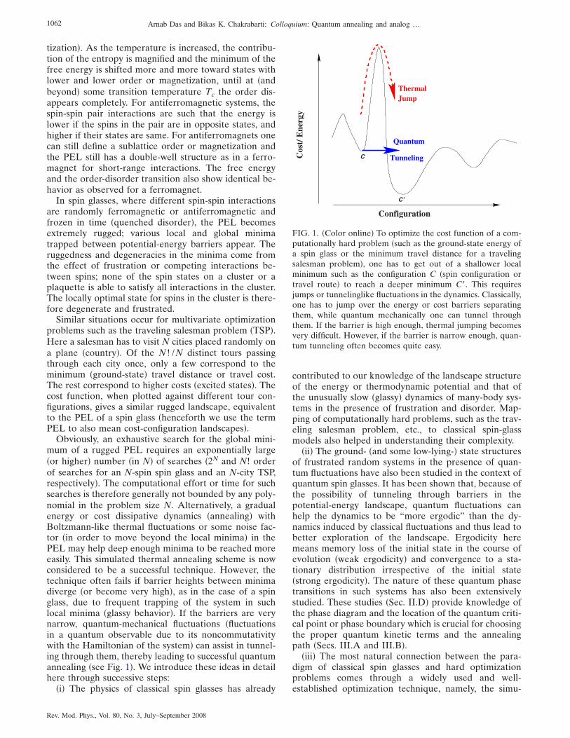
Obviously, an exhaustive search for the global mini-mum of a rugged PEL requires an exponentially large�or higher� number �in N� of searches �2N and N! orderof searches for an N-spin spin glass and an N-city TSP,respectively�. The computational effort or time for suchsearches is therefore generally not bounded by any poly-nomial in the problem size N. Alternatively, a gradualenergy or cost dissipative dynamics �annealing� withBoltzmann-like thermal fluctuations or some noise fac-tor �in order to move beyond the local minima� in thePEL may help deep enough minima to be reached moreeasily. This simulated thermal annealing scheme is nowconsidered to be a successful technique. However, thetechnique often fails if barrier heights between minimadiverge �or become very high�, as in the case of a spinglass, due to frequent trapping of the system in suchlocal minima �glassy behavior�. If the barriers are verynarrow, quantum-mechanical fluctuations �fluctuationsin a quantum observable due to its noncommutativitywith the Hamiltonian of the system� can assist in tunnel-ing through them, thereby leading to successful quantumannealing �see Fig. 1�. We introduce these ideas in detailhere through successive steps:

�i� The physics of classical spin glasses has already

contributed to our knowledge of the landscape structureof the energy or thermodynamic potential and that ofthe unusually slow �glassy� dynamics of many-body sys-tems in the presence of frustration and disorder. Map-ping of computationally hard problems, such as the trav-eling salesman problem, etc., to classical spin-glassmodels also helped in understanding their complexity.

�ii� The ground- �and some low-lying-� state structuresof frustrated random systems in the presence of quan-tum fluctuations have also been studied in the context ofquantum spin glasses. It has been shown that, because ofthe possibility of tunneling through barriers in thepotential-energy landscape, quantum fluctuations canhelp the dynamics to be “more ergodic” than the dy-namics induced by classical fluctuations and thus lead tobetter exploration of the landscape. Ergodicity heremeans memory loss of the initial state in the course ofevolution �weak ergodicity� and convergence to a sta-tionary distribution irrespective of the initial state�strong ergodicity�. The nature of these quantum phasetransitions in such systems has also been extensivelystudied. These studies �Sec. II.D� provide knowledge ofthe phase diagram and the location of the quantum criti-cal point or phase boundary which is crucial for choosingthe proper quantum kinetic terms and the annealingpath �Secs. III.A and III.B�.

�iii� The most natural connection between the para-digm of classical spin glasses and hard optimizationproblems comes through a widely used and well-established optimization technique, namely, the simu-

C’

C

Configuration

Quantum

Tunneling

ThermalJump

Cos

t/E

nerg

y

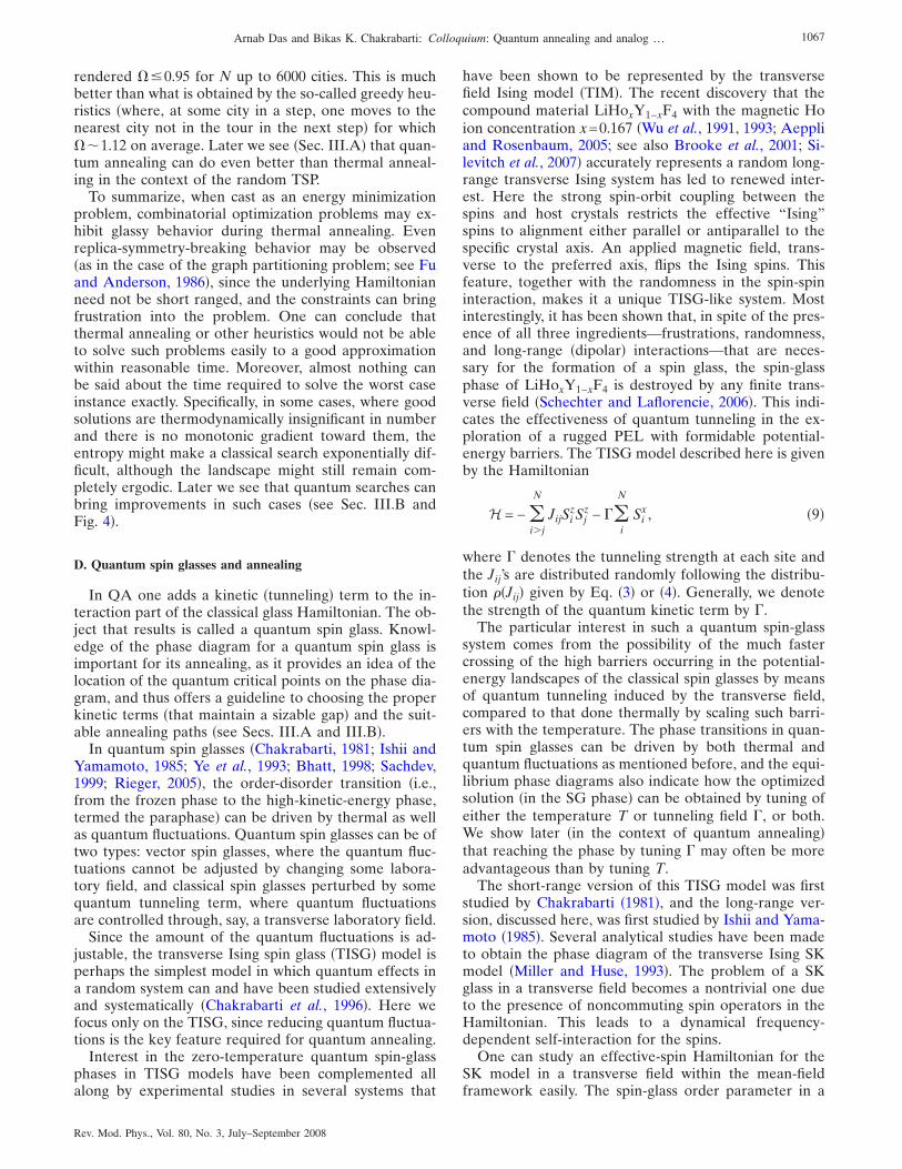
FIG. 1. �Color online� To optimize the cost function of a com-putationally hard problem �such as the ground-state energy ofa spin glass or the minimum travel distance for a travelingsalesman problem�, one has to get out of a shallower localminimum such as the configuration C �spin configuration ortravel route� to reach a deeper minimum C�. This requiresjumps or tunnelinglike fluctuations in the dynamics. Classically,one has to jump over the energy or cost barriers separatingthem, while quantum mechanically one can tunnel throughthem. If the barrier is high enough, thermal jumping becomesvery difficult. However, if the barrier is narrow enough, quan-tum tunneling often becomes quite easy.

1062 Arnab Das and Bikas K. Chakrabarti: Colloquium: Quantum annealing and analog …

Rev. Mod. Phys., Vol. 80, No. 3, July–September 2008

lated annealing algorithm as discussed earlier. The pos-sibility of quantum tunneling through classicallyimpenetrable barriers, as indicated by studies of quan-tum spin glasses, naturally suggests an elegant and oftenmore effective alternative to simulated annealing.

In quantum annealing, one has a classical Hamil-tonian �or a multivariate cost function viewed as thesame� to be optimized, to which one adds a �noncom-muting� quantum kinetic term and reduces it from a highinitial value to zero eventually. This reduction, whendone completely adiabatically, assures that the groundstate of the classical glass is reached at the end, assumingthat there is no crossing of energy levels with the groundstate in the course of evolution, and provided that thestarting state was the ground state of the initial Hamil-tonian. To start with, the tunneling field is much higherthan the interaction term, so the ground state �a uniformsuperposition of all classical configurations� is triviallyrealizable. Simulations demonstrate that quantum an-nealing can occasionally help reach the ground state of acomplex glassy system much faster than done using ther-mal annealing �discussed later in Sec. III�. An experi-ment comparing classical and quantum annealing for aspin glass also shows that the relaxations in the course ofquantum annealing are often much faster than thoseduring the corresponding classical annealing, as dis-cussed in Sec. III.D. What makes quantum annealingfundamentally different from classical annealing is thenonlocal nature �Sec. III� and its higher tunneling ability�Secs. II.D and III.C�.

Quantum annealing thus permits a realization of ana-log quantum computation, which is an independent andpowerful complement to digital quantum computation,where discrete unitary transformations are implementedthrough quantum logic gates.

II. OPTIMIZATION AND ANNEALING

A. Combinatorial optimization problems

The occurrence of multivariate optimization problemsis ubiquitous in our life, wherever one has to choose thebest bargain from a host of available options that de-pend on many independent factors. In many cases, sucha task can be cast as a problem of minimizing a givencost or energy function H�S1 ,S2 , . . . ,SN� with respect toN variables S1 ,S2 , . . . ,SN �sometimes subject to someconstraints�. The task is to find a set of values for thesevariables �a configuration� for which the function H��Si��has the minimum value �cf. Fig. 1�. In many importantoptimization problems, the set of feasible configurationsfrom which an optimum is to be chosen is a finite set �forfinite N�. In such a case, we say that the problem iscombinatorial in nature. If the variables Si are discreteand each takes a finite number of values, then the prob-lem is a combinatorial one. Moreover, certain problemswith continuous variables �such as linear programmingproblems� can also be reduced to combinatorial prob-lems �Papadimitriou and Steiglitz, 1998�. Here we focuson this type of optimization problem, and assume that

we have to minimize H��Si�� with respect to the discreteset of variables Si.

An optimization problem is said to belong to the classP �P for polynomial�, if it can be solved in polynomialtime �i.e., the evaluation time varies as some polynomialin N� using polynomially �in N, again� bound resources�computer space, processors, etc.�. The existence of sucha polynomial bound on the evaluation time is sometimesinterpreted as the “easiness” of the problem. However,many important optimization problems seem to fall out-side this class, such as the traveling salesman problem�see Sec. II.C.2�.

There is another important class of problems whichcan be solved in polynomial time by nondeterministicmachines. This class is the nondeterministic polynomial�NP� class �Garey and Johnson, 1979�. P is includedcompletely in the NP class, since a deterministic Turingmachine is a special case of nondeterministic Turing ma-chines. Unlike a deterministic machine, which takes aspecific step deterministically at each instant �and hencefollows a single computational path�, a nondeterministicmachine has a host of different “allowed” steps at itsdisposal at every instant. At each instant it explores allallowed steps and if any one of them leads to the goal,the job is considered to be done. Thus it explores inparallel many paths �whose number varies roughly expo-nentially with time� and checks if any one of themreaches the goal.

Among the NP problems, there are certain problems�known as NP-complete problems� which are such thatany NP problem can be “reduced” to them using a poly-nomial algorithm. The famous 3-SAT problem �see Sec.III.A.3� is a representative of the class. This roughlymeans that, if one has a routine to solve an NP-completeproblem of size N, then using that routine one can solveany NP problem at the cost of an extra overhead in timethat varies only polynomially with N. Problems in thisclass are considered to be hard, since so far a generalnondeterministic machine cannot be simulated by a de-terministic Turing machine �or any sequential computerwith polynomially bound resources� without an expo-nential growth of execution time. In fact, it is widelybelieved �though not proved yet� that it is impossible todo so �i.e., P�NP� in principle. However, assuming thisto be true, one can show that there are indeed problemsin the NP class that are neither NP complete nor P�Garey and Johnson, 1979�.

B. Statistical mechanics of the optimization problems andthermal annealing

There are some excellent deterministic algorithms forsolving certain optimization problems exactly �Pa-padimitriou and Steiglitz, 1998; Hartmann and Rieger,2002�. These algorithms are, however, small in numberand are strictly problem specific. For NP or harder prob-lems, only approximate results can be found using thesealgorithms in polynomial time. These approximate algo-rithms too are also strictly problem specific, in the sense

1063Arnab Das and Bikas K. Chakrabarti: Colloquium: Quantum annealing and analog …


that, if one can solve a certain NP-complete problem upto a certain approximation using some polynomial algo-rithm, that does not ensure that one can solve all otherNP problems using the same algorithm up to the saidapproximation in polynomial time.

Exact algorithms being scarce, one has to look forheuristic algorithms, which are algorithms based on cer-tain intuitive moves, without any guarantee on either theaccuracy or the run time for the worst case instance.However, these algorithms are generally easy to formu-late and are effective in solving most instances of theintended problems. A general approach toward formu-lating such approximate heuristics may be based on sto-chastic �randomized� iterative improvements. The mostcommon starting point in this family is the local minimi-zation algorithm. In this algorithm one starts with a ran-dom configuration C0 and makes some local changes inthe configuration following some prescription �stochasticor deterministic� to generate a new configuration C1 andcalculates the corresponding change in the cost. If thecost is lowered by the change, then the new configura-tion C1 is adopted. Otherwise the old configuration isretained. Then in the next step a new local change isattempted again, and so on. This reduces the coststeadily until a configuration is reached that minimizesthe cost locally. This means that no further lowering ofcost is possible by changing this configuration using anyof the prescribed local moves. The algorithm essentiallystops there. But generally, in most optimization prob-lems �as in spin glasses�, there occur many local minimain the cost-configuration landscape and they are mostlyfar above the global minimum �see Fig. 1�. It is likelythat the algorithm therefore gets stuck in one of themand ends up with a poor approximation. One can thenstart afresh with some new initial configuration and endup with another local minimum. After repeating thisseveral times, each time with a new initial configuration,one may choose the best result from them. But a muchbetter idea would be to somehow get out of shallowlocal minima. One can introduce some fluctuations ornoise in the process so that the movement is not alwaystoward lower-energy configurations, but there is also afinite probability to go to higher-energy configurations�the higher the final state energy, the lower the probabil-ity to move there�, and consequently chances appear toget out of the shallow local minima. Initially, strongfluctuations are adopted �i.e., the probability to go tohigher-energy configurations is relatively high� andslowly the fluctuations are reduced until finally they areturned off completely. In the meantime the system gets afair opportunity to explore the landscape more exhaus-tively and settle into a reasonably deep cost or energyminimum. Kirkpatrick et al. �1983� suggested an elegantmethod: A fluctuation is implemented by introducing an“artificial” temperature T into the problem such that thetransition probability from a configuration Ci to a con-figuration Cf is given by min�1,exp− ��if /T��, where �if=Ef−Ei, with Ek denoting the cost or energy of the con-figuration Ck. A corresponding Monte Carlo dynamics isdefined, say, based on detailed balance, and the thermal

relaxation of the system is simulated. In the course ofsimulation, the noise factor T is reduced slowly from ahigh initial value to zero, following some annealingschedule. At the end of the simulation one is expected toend up with a configuration whose cost is a reasonableapproximation of the globally minimum one. If the tem-perature is decreased slowly enough, say,

T�t� � N/ln t , �1�

where t denotes the cooling time and N is the systemsize, then the global minimum is attained with certaintyin the limit t→� �Geman and Geman, 1984�. Evenwithin a finite time and with a faster cooling rate, onecan achieve a reasonably good approximation �a crystalwith only a few defects� in practice. This simulated an-nealing method is now used extensively by engineers fordevising real-life optimization algorithms. We refer tothis as classical annealing �CA�, to distinguish it fromquantum annealing �QA� which employs quantum fluc-tuations. It is important to note that, although in thistype of stochastic algorithm the system has many differ-ent steps with their corresponding probabilities at its dis-posal, it finally takes up a single one, chosen, say, bytossing coins, and thus finally follows a single �stochasti-cally selected� path. Hence it is not equivalent to a non-deterministic machine, where all allowed paths arechecked in parallel at every time step.

As mentioned already, many combinatorial optimiza-tion problems can be cast into the problem of finding theground state of some classical �spin-glass-like� Hamil-tonian H��Si��. One can therefore analyze the problemusing statistical mechanics to apply physical techniqueslike simulated annealing. If one naively takes the num-ber of variables N as the size, then the entropy and theenergy are often found to scale differently with N andapplying standard thermodynamic arguments becomesdifficult. One needs to scale temperature and some otherquantities properly with N so that one can talk in termsof concepts like free-energy minimization, etc. More-over, the constraints present in the problems are oftendifficult to take into account.

C. Spin glasses and optimization

1. Finding the ground states of classical spin glasses

As mentioned already, the difficulty faced by a physi-cally motivated optimization heuristic �one that followsphysical relaxation dynamics, classical or quantum, tosearch for the solution� in finding the solution of a hardoptimization problem is similar to that faced by a glassysystem in reaching its ground state. In fact, finding theground state of a spin glass is an important class of com-binatorial optimization problem, which includes an NP-complete problem �Barahona, 1982�, and many other ap-parently different ones �such as the traveling salesmanproblem� can be recast in this form. Hence, we discusshere the nature of the spin-glass phase and the difficultyin reaching its ground state.



The interaction energy of a typically random and frus-trated Ising spin glass �Binder and Young, 1986; Dot-senko, 2001; Nishimori, 2001� may be represented by aHamiltonian of the form

H = − �i�j

N

JijSiSj, �2�

where Si denote the Ising spins and Jij the interactionsbetween them. The Jij’s here are quenched variableswhich vary randomly in both sign and magnitude follow-ing some distribution ��Jij�. The typical distributions arethe �zero-mean� Gaussian distribution of positive andnegative Jij values,

��Jij� = A exp�−Jij

2

2J2 , �3�

and the binary distribution,

��Jij� = p��Jij − J� + �1 − p��Jij + J� , �4�

with probability p of having a +J bond, and 1−p of hav-ing a −J bond. Two well-studied models are theSherrington-Kirkpatrick �SK� model �Sherrington andKirkpatrick, 1975� and the Edwards-Anderson �EA�model �Edwards and Anderson, 1975�. In the SK modelthe interactions are infinite ranged and for the sake ofextensivity �for the rules of equilibrium thermodynamicsto be applicable, the energy should be proportional tothe volume, or its equivalent that defines the systemsize� one has to scale J1/�N, while in the EA model,the interactions are between nearest neighbors only. Forboth of them, however, ��Jij� is Gaussian; A= �N /2�J2�1/2 for normalization in the SK model.

Freezing �temperatures below Tc� is characterized bysome nonzero value of the thermal average of the mag-netization at each site �local ordering�. However, sincethe interactions are random and competing, the spatialaverage of single-site magnetization �below Tc� is zero.Above Tc, both the spatial and temporal averages of thesingle-site magnetization vanish. A relevant order pa-rameter for this freezing to occur is therefore

q =1

N�i

N

�Si T2 �5�

�with the overbar denoting the average over disorders�the distribution of Jij� and �¯ T denoting the thermalaverage�. Here q�0 for T�Tc, while q=0 for T�Tc. Asshown in the following, the existence of a unique orderparameter q indicates ergodicity.

In the spin-glass phase �T�Tc�, the whole free-energylandscape is divided �cf. Fig. 1� into many valleys �localminima of the free energy� separated by high free-energy barriers. Thus the system, once trapped in a val-ley, remains there for a long time. The spins of such aconfined system are allowed to explore only a restricted�and correlated� part of the configuration space, andthus “freeze” with a magnetization that characterizes thestate �valley� locally.

To date two competing pictures continue to representthe physics of the spin glasses. The mean-field picture ofreplica symmetry breaking is valid for infinite-rangedspin-glass systems like the SK spin glass. In this picture,below the glass transition temperature Tc, the barriersseparating the valleys in the free-energy landscape actu-ally diverge �in the limit N→��, giving rise to a diverg-ing time scale for the confinement of the system in anysuch valley once the system gets there somehow. Thismeans there is a loss of ergodicity in the thermal dynam-ics of the system at T�Tc. Thus one needs a distributionP�q� of order parameters, instead of a single order pa-rameter, to characterize the whole landscape, as emergesnaturally from the replica symmetry-breaking ansatz ofParisi �1980�. To be a bit more quantitative, imagine thattwo identical replicas �having exactly the same set ofJij’s� of a spin-glass sample are allowed to relax ther-mally below Tc, starting from two different random�paramagnetic� initial states. Then these two replicas �la-beled by and , say� will settle in two different valleys,each characterized by a local value of the order param-eter and the corresponding overlap parameters q,which have a sample-specific distribution

PJ�q� = �,

e−�F+F�/T��q − q� ,

P�q� =� �i�j

dJij��Jij�PJ�q� . �6�

Here the subscript J denotes a particular sample with agiven realization of quenched random interactions �Jij’s�between spins, and finally, by averaging PJ�q� over thedisorder distribution ��J� in Eq. �2� or �3�, one gets P�q�.Physically, P�q� gives the probability distribution for thetwo pure states to have an overlap q, assuming that theprobability of reaching any pure state starting from arandom �high-temperature� state is proportional to thethermodynamic weight exp�−F� of the state .

The other picture of the physics of spin glasses is dueto the droplet model of short-range spin glasses �Brayand Moore, 1984; Fisher and Huse, 1986�, where there isno divergence in the typical free-energy barrier height,and the relevant time scale is taken to be that of crossingthe free-energy barrier of formation of a typical dropletof same �all up or all down� spins. Based on a certainscaling ansatz, this picture leads to a logarithmically de-caying �with time� self-correlation function for the spinsbelow the freezing temperature Tc.

The validity of the mean-field picture �of replica sym-metry breaking� in the context of real-life spin glasses,where interactions are essentially short range, is far fromsettled �see, e.g., Marinari et al., 1998; Moore et al., 1998;Krzakala et al., 2001; Gaviro et al., 2006�. However, theeffective Hamiltonian �cost function� for many other op-timization problems may contain long-range interactionsand may even show the replica symmetry-breaking be-havior shown in the graph partitioning problem �Fu andAnderson, 1986�. Of course, no result of QA for such asystem �for which replica symmetry breaking is shown



explicitly� has been reported yet. The successes of QAreported so far are mostly for short-range systems. Thusthe scope of quantum annealing in those long-range sys-tems still remains an interesting open question.

2. The traveling salesman problem

In the traveling salesman problem, there are N citiesplaced randomly in a country, with a definite metric tocalculate the intercity distances. A salesman has to makea tour to cover every city and finally come back to thestarting point. The problem is to find the tour of mini-mum length. An instance of the problem is given by aset �dij ; i , j=1,N�, where dij indicates the distance be-tween the ith and jth cities, or equivalently the cost forgoing from the former to the latter. We mainly focus onthe results of the symmetric case, where dij=dji. Theproblem can be cast into a form where one minimizes anIsing Hamiltonian under some constraints, as shown be-low. A tour can be represented by an N�N matrix Twith elements either 0 or 1. In a given tour, if the city j isvisited immediately after visiting city i, then Tij=1 orelse Tij=0. Generally, an additional constraint is im-posed that each city has to be visited once and only oncein a tour. Any valid tour with the above restriction maybe represented by a T matrix whose each row and eachcolumn has one and only one element equal to 1 and therest are all 0’s. For a symmetric metric, a tour and itsreverse have the same length, and it is more convenient

to work with an undirected tour matrix U= 12 �T+ T�,

where T, the transpose of T, represents the reverse ofthe tour given by T. Clearly, U must be a symmetricmatrix having two and only two distinct entries equal to1 in every row and every column, with no two rows ortwo columns identical. In terms of the Uij’s, the length ofa tour can be represented by

H =12 �

i,j=1

N

dijUij. �7�

One can rewrite the above Hamiltonian in terms of Isingspins Sij’s as

HTSP =12 �

i,j=1

N

dij�1 + Sij�

2, �8�

where Sij=2Uij−1 are the Ising spins. The Hamiltonianis similar to that of noninteracting Ising spins on anN�N lattice, with random fields dij on the lattice points�i , j�. The frustration is introduced by the global con-straints on the spin configurations in order to conformwith the structure of the matrix U discussed above. Theproblem is to find the ground state of the Hamiltoniansubject to these constraints. There are N2 Ising spins,which can assume 2N2

configurations in the absence ofany constraint, but the constraint here reduces the num-ber of valid configurations to the number of distincttours, which is �N ! � /2N.

Two distinct classes of the TSP are mainly studied,one with a Euclidean dij in finite dimensions �where thedij are strongly correlated through triangle inequalities,which means that, for any three cities A, B, and C, thesum of any two of the sides AB, BC, and CA must begreater than the remaining one�, and the other with ran-dom dij in infinite dimension.

In the first case, N cities are uniformly distributedwithin a hypercube in a d-dimensional Euclidean space.Finding a good approximation for large N is easier inthis case, since the problem is finite ranged. Here ad-dimensional neighborhood is defined for each city, andthe problem can be solved by dividing the whole hyper-cube into a number of smaller pieces and then searchingfor the least path within each smaller part and joiningthem back together. The correction to obtain the trueleast path will be due to the unoptimized connectionsacross the boundaries of the subdivisions. For a suitablymade division �not too small�, this correction will be onthe order of the surface-to-volume ratio of each division,and thus will tend to zero in the N→� limit. Thismethod, known as “divide and conquer,” forms a rea-sonable strategy for solving approximately such finite-range optimization problems �including finite-range spinglasses� in general. In the second case, the dij’s are as-signed completely randomly, with no geometric �e.g.,Euclidean� correlation between them. The problem inthis case becomes more like a long-range spin glass. Aself-avoiding walk representation of the problem hasbeen made using an m-component vector field, and thereplica analysis has been done �Mezard et al., 1987� forfinite temperature, assuming the replica-symmetry an-satz to hold. Moreover, true breaking of ergodicity mayoccur only in infinite systems, not in any finite instanceof the problem. The results, when extrapolated to zerotemperature, do not disagree much with the numericalresults �Mezard et al., 1987�. The stability of a replica-symmetric solution has not yet been proven for the low-temperature region. However, the numerical results forthermal annealing, for instance of size N=60–160,yielded many near-optimal tours, and the correspondingoverlap analysis shows a sharply peaked distribution,whose width decreases steadily with increase in N. Thisindicates the existence of a replica-symmetric phase forthe system �Mezard et al., 1987�.

An analytical bound on the average �normalized byN1/2� value of the optimal path length per city �� calcu-lated for the TSP on a two-dimensional Euclidean planehas been found to be 5/8��0.92 �Bearwood et al.,1959�. Careful scaling analysis of the numerical resultsobtained indicates the lower bound to be close to 0.72�Percus and Martin, 1996; Chakraborti and Chakrabarti,2000�.

Simulated �thermal� annealing of a Euclidean TSP ona square having length N1/2 �which render the averagenearest-neighbor distance independent of N� has beenreported �Kirkpatrick et al., 1983�. In this choice oflength unit, the optimal tour length per step �� be-comes independent of N for large N. Thermal annealing



rendered � 0.95 for N up to 6000 cities. This is muchbetter than what is obtained by the so-called greedy heu-ristics �where, at some city in a step, one moves to thenearest city not in the tour in the next step� for which�1.12 on average. Later we see �Sec. III.A� that quan-tum annealing can do even better than thermal anneal-ing in the context of the random TSP.

To summarize, when cast as an energy minimizationproblem, combinatorial optimization problems may ex-hibit glassy behavior during thermal annealing. Evenreplica-symmetry-breaking behavior may be observed�as in the case of the graph partitioning problem; see Fuand Anderson, 1986�, since the underlying Hamiltonianneed not be short ranged, and the constraints can bringfrustration into the problem. One can conclude thatthermal annealing or other heuristics would not be ableto solve such problems easily to a good approximationwithin reasonable time. Moreover, almost nothing canbe said about the time required to solve the worst caseinstance exactly. Specifically, in some cases, where goodsolutions are thermodynamically insignificant in numberand there is no monotonic gradient toward them, theentropy might make a classical search exponentially dif-ficult, although the landscape might still remain com-pletely ergodic. Later we see that quantum searches canbring improvements in such cases �see Sec. III.B andFig. 4�.

D. Quantum spin glasses and annealing

In QA one adds a kinetic �tunneling� term to the in-teraction part of the classical glass Hamiltonian. The ob-ject that results is called a quantum spin glass. Knowl-edge of the phase diagram for a quantum spin glass isimportant for its annealing, as it provides an idea of thelocation of the quantum critical points on the phase dia-gram, and thus offers a guideline to choosing the properkinetic terms �that maintain a sizable gap� and the suit-able annealing paths �see Secs. III.A and III.B�.

In quantum spin glasses �Chakrabarti, 1981; Ishii andYamamoto, 1985; Ye et al., 1993; Bhatt, 1998; Sachdev,1999; Rieger, 2005�, the order-disorder transition �i.e.,from the frozen phase to the high-kinetic-energy phase,termed the paraphase� can be driven by thermal as wellas quantum fluctuations. Quantum spin glasses can be oftwo types: vector spin glasses, where the quantum fluc-tuations cannot be adjusted by changing some labora-tory field, and classical spin glasses perturbed by somequantum tunneling term, where quantum fluctuationsare controlled through, say, a transverse laboratory field.

Since the amount of the quantum fluctuations is ad-justable, the transverse Ising spin glass �TISG� model isperhaps the simplest model in which quantum effects ina random system can and have been studied extensivelyand systematically �Chakrabarti et al., 1996�. Here wefocus only on the TISG, since reducing quantum fluctua-tions is the key feature required for quantum annealing.

Interest in the zero-temperature quantum spin-glassphases in TISG models have been complemented allalong by experimental studies in several systems that

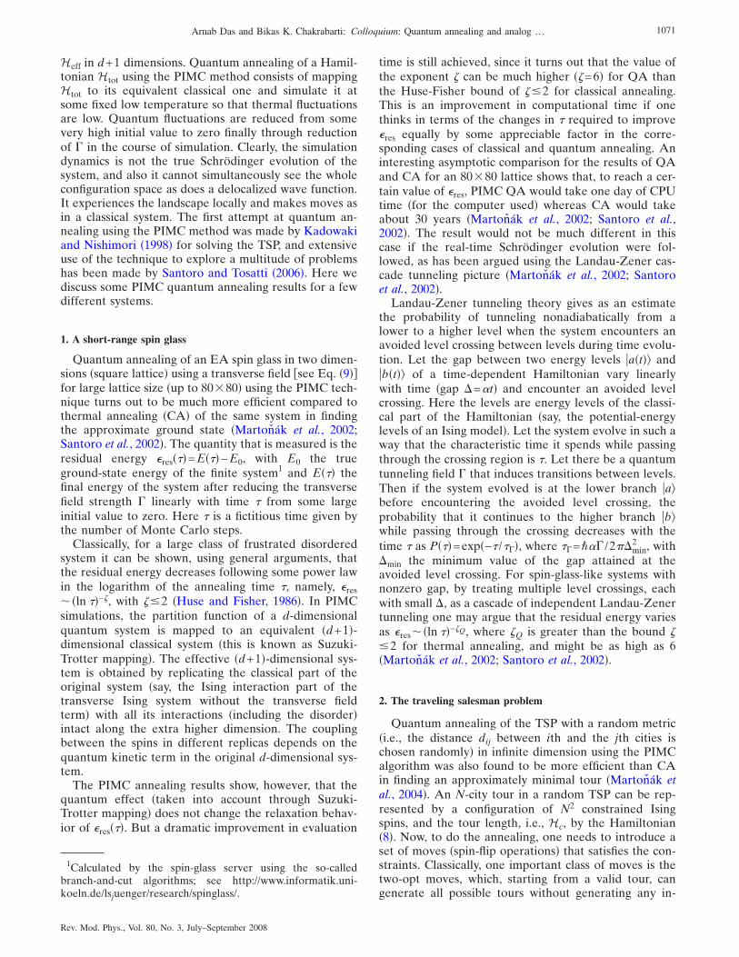
have been shown to be represented by the transversefield Ising model �TIM�. The recent discovery that thecompound material LiHoxY1−xF4 with the magnetic Hoion concentration x=0.167 �Wu et al., 1991, 1993; Aeppliand Rosenbaum, 2005; see also Brooke et al., 2001; Si-levitch et al., 2007� accurately represents a random long-range transverse Ising system has led to renewed inter-est. Here the strong spin-orbit coupling between thespins and host crystals restricts the effective “Ising”spins to alignment either parallel or antiparallel to thespecific crystal axis. An applied magnetic field, trans-verse to the preferred axis, flips the Ising spins. Thisfeature, together with the randomness in the spin-spininteraction, makes it a unique TISG-like system. Mostinterestingly, it has been shown that, in spite of the pres-ence of all three ingredients—frustrations, randomness,and long-range �dipolar� interactions—that are neces-sary for the formation of a spin glass, the spin-glassphase of LiHoxY1−xF4 is destroyed by any finite trans-verse field �Schechter and Laflorencie, 2006�. This indi-cates the effectiveness of quantum tunneling in the ex-ploration of a rugged PEL with formidable potential-energy barriers. The TISG model described here is givenby the Hamiltonian

H = − �i�j

N

JijSizSj

z − ��i

N

Six, �9�

where � denotes the tunneling strength at each site andthe Jij’s are distributed randomly following the distribu-tion ��Jij� given by Eq. �3� or �4�. Generally, we denotethe strength of the quantum kinetic term by �.

The particular interest in such a quantum spin-glasssystem comes from the possibility of the much fastercrossing of the high barriers occurring in the potential-energy landscapes of the classical spin glasses by meansof quantum tunneling induced by the transverse field,compared to that done thermally by scaling such barri-ers with the temperature. The phase transitions in quan-tum spin glasses can be driven by both thermal andquantum fluctuations as mentioned before, and the equi-librium phase diagrams also indicate how the optimizedsolution �in the SG phase� can be obtained by tuning ofeither the temperature T or tunneling field �, or both.We show later �in the context of quantum annealing�that reaching the phase by tuning � may often be moreadvantageous than by tuning T.

The short-range version of this TISG model was firststudied by Chakrabarti �1981�, and the long-range ver-sion, discussed here, was first studied by Ishii and Yama-moto �1985�. Several analytical studies have been madeto obtain the phase diagram of the transverse Ising SKmodel �Miller and Huse, 1993�. The problem of a SKglass in a transverse field becomes a nontrivial one dueto the presence of noncommuting spin operators in theHamiltonian. This leads to a dynamical frequency-dependent self-interaction for the spins.

One can study an effective-spin Hamiltonian for theSK model in a transverse field within the mean-fieldframework easily. The spin-glass order parameter in a



classical SK model is given by a random mean field h�r�having a Gaussian distribution �see Binder and Young,1986�,

q = �−�

+�

dr e−r2/2 tanh2�hz�r�/T�, hz�r� = J�qr + hz,

�10�

where hz denotes the external field �in the z direction�,with the mean field h�r� also in the same direction. Inthe presence of the transverse field, as in Eq. �9�, h�r�has components in both the z and x directions,

h� �r� = − hz�r�z − �x, h�r� = �hz�r�2 + �2, �11�

and one replaces the ordering term tanh2�h�r� /T� in Eq.�10� by its component ��hz�r� � / �h�r� � �2tanh2��h�r� � /T� inthe z direction. Setting hz=0 and q→0, one gets thephase boundary equation as �see Chakrabarti et al.,1996�

�

J= tanh��

T . �12�

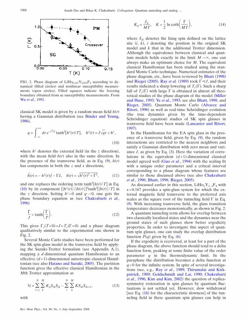
This gives �c�T=0�=J=Tc��=0� and a phase diagramqualitatively similar to the experimental one shown inFig. 2.

Several Monte Carlo studies have been performed forthe SK spin-glass model in the transverse field by apply-ing the Suzuki-Trotter formalism �see Appendix A.1�,mapping a d-dimensional quantum Hamiltonian to aneffective �d+1�-dimensional anisotropic classical Hamil-tonian �see also Hatano and Suzuki, 2005�. The partitionfunction gives the effective classical Hamiltonian in theMth Trotter approximation as

H = �i�j

N

�k

M

KijSikSjk − �i

N

�k

M

KSikSik+1, �13�

with

Kij =Jij

MT, K =

12

ln coth� �

MT , �14�

where Sik denotes the Ising spin defined on the latticesite �i, k�, i denoting the position in the original SKmodel and k that in the additional Trotter dimension.Although the equivalence between classical and quan-tum models holds exactly in the limit M→�, one canalways make an optimum choice for M. The equivalentclassical Hamiltonian has been studied using the stan-dard Monte Carlo technique. Numerical estimates of thephase diagram, etc., have been reviewed by Bhatt �1998�and Rieger �2005�. Ray et al. �1989� took ��J, and theirresults indicated a sharp lowering of Tc��. Such a sharpfall of Tc�� with large � is obtained in almost all theo-retical studies of the phase diagram of the model �Millerand Huse, 1993; Ye et al., 1993; see also Bhatt, 1998, andRieger, 2005�. Quantum Monte Carlo �Alvarez andRitort, 1996� as well as real-time Schrödinger evolution�the true dynamics given by the time-dependentSchrödinger equation� studies of SK spin glasses intransverse field have been made �Lancaster and Ritort,1997�.

In the Hamiltonian for the EA spin glass in the pres-ence of a transverse field, given by Eq. �9�, the randominteractions are restricted to the nearest neighbors andsatisfy a Gaussian distribution with zero mean and vari-ance J, as given by Eq. �3�. Here the variation of corre-lations in the equivalent �d+1�-dimensional classicalmodel agreed well �Guo et al., 1994� with the scaling fitwith a unique order parameter and a critical intervalcorresponding to a phase diagram whose features aresimilar to those discussed above �see also Chakrabartiet al., 1996; Bhatt, 1998; Rieger, 2005�.

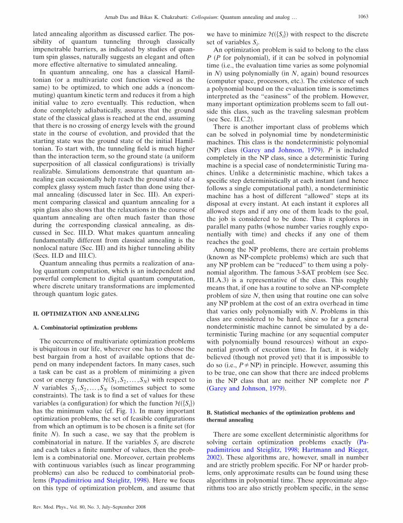
As discussed earlier in this section, LiHoxY1−xF4 withx=0.167 provides a spin-glass system for which the ex-ternal magnetic field transverse to the preferred axisscales as the square root of the tunneling field � in Eq.�9�. With increasing transverse field, the glass transitiontemperature decreases monotonically, as shown in Fig. 2.

A quantum tunneling term allows for overlap betweentwo classically localized states and the dynamics near theground states of such glasses show better ergodicityproperties. In order to investigate this aspect of quan-tum spin glasses, one can study the overlap distributionfunction P�q� given by Eq. �6�.

If the ergodicity is recovered, at least for a part of thephase diagram, the above function should tend to a deltafunction form, peaking at some finite value of the orderparameter q in the thermodynamic limit. In theparaphase the distribution becomes a delta function atq=0 for the infinite system. In spite of several investiga-tions �see, e.g., Ray et al., 1989; Thirumalai and Kirk-patrick, 1989; Goldschmidt and Lai, 1990; Chakrabartiet al., 1996; Kim and Kim, 2002� the question of replica-symmetry restoration in spin glasses by quantum fluc-tuations is not settled yet. However, slow withdrawal�see Eq. �16� for the characteristic slowness� of the tun-neling field in these quantum spin glasses can help in

FIG. 2. Phase diagram of LiHo0.167Y0.833F4 according to dy-namical �filled circles� and nonlinear susceptibility measure-ments �open circles�. Filled squares indicate the freezingboundary obtained from ac susceptibility measurements. FromWu et al., 1993.



annealing the system close to the ground state of theclassical spin glass eventually, as described in the nextsection.

III. QUANTUM ANNEALING

In the previous sections we have seen how thermalfluctuations can be utilized to devise fast heuristics tofind an approximate ground state of a glassy system, orequivalently a near-optimal solution to the combinato-rial problem, whose cost-configuration landscape hasglassy behavior due to the occurrence of many localminima. There are two aspects of an optimization prob-lem which might render thermal annealing an ineffectiveone. First, in a glassy landscape, there may exist high-cost or -energy barriers around local minima which donot correspond to a reasonably low cost �see Fig. 1�. Inthe case of infinite-range problems, these barriers mightbe proportional to the system size N, and thus diverge inthermodynamic limit. Thus many unsatisfactory localminima might occur, any of which can trap the systemfor a long time �which actually diverges in the thermo-dynamic limit for infinite-range systems� in the course ofannealing. The second problem is the entropy itself. Thenumber of configurations grows fast with the number ofvariables �roughly exponentially; n Ising spins can be in2n configurations�, and a classical system can assumeonly one configuration at a time; unless there is a gradi-ent that broadly guides the system toward the globalminimum from any point in the configuration space, thesearch has to involve visiting a substantial fraction ofconfigurations. Thus a PEL without a guiding gradientposes a problem which is exponential or higher order incomplexity �depending on how the size of the configura-tion space scales with the system size N�, and the CAalgorithms can do no better than a random search algo-rithm. This is the case for the golf-course-type potential-energy landscape, where there is a sharp potential mini-mum on a completely flat PEL �see Sec. III.B, Fig. 4�.One can imagine that quantum mechanics might havesolutions to both these problems, at least to some extent.This is because quantum mechanics can introduce clas-sically unlikely tunneling paths even through very highbarriers if they are narrow enough �Ray et al., 1989; seealso Apolloni et al., 1989, 1990�. This can solve the er-godicity problem to some extent, as discussed earlier.Even in places where ergodicity breaking does not takeplace in the true sense, once the energy landscape con-tains high enough barriers �especially for infinite-rangedquenched interactions�, quantum tunneling may providemuch faster relaxation to the ground state �Martonáket al., 2002; Santoro et al., 2002; see also Santoro andTosatti, 2007; Somma et al., 2007�. In addition, aquantum-mechanical wave function can delocalize overthe whole configuration space �i.e., over the potential-energy landscape� if the kinetic energy term is highenough. Thus it can actually “see” the whole landscapesimultaneously at some stage of annealing. These twoaspects can be expected to improve the search processwhen employed properly. In fact, such improvements

can be achieved in certain situations, though quantummechanics is not a panacea for all such problems as er-godicity breaking, spin-glass behavior, etc., and certainlyhas its own inherent limitations. What is intriguing is thefact that the limitations due to the quantum nature of analgorithm are inherently different from those faced byits classical counterpart, and thus it is not yet clear ingeneral which is better when. Here we discuss resultsregarding quantum heuristics and some of their generalaspects that are understood so far. For more detailedreviews of the subject we refer the reader to articles byDas and Chakrabarti �2005� and Santoro and Tosatti�2006�.

Some basic aspects of QA can be understood from thesimple case of QA in the context of a double-well po-tential �Battaglia, Stella, et al., 2005; Stella et al., 2005�.Typically a particle in a double well consisting of a shal-lower but wider well and a deeper but narrower well isannealed �it is likely that the deeper well, i.e., the targetstate, is narrower, otherwise searching becomes easiereven classically�. The kinetic energy �inverse mass� istuned from a very high value to zero linearly within atime �. For a very high value of initial kinetic energy, thewave function, which is the ground state, is delocalizedmore or less over the whole double well. As kinetic en-ergy is reduced but still quite high, the ground state cor-responds to a more pronounced peak on the shallowerminimum, since it is wider. This is because at this stage,to obtain the minimal �ground-state� energy, it is moreeffective to minimize the kinetic energy by localizationover a wider space, rather than minimizing the potentialenergy by localizing in the deeper well. However, as thekinetic energy is reduced further, the potential energyterm dominates, and the ground state has a taller peakaround the deeper minimum. The evolving wave func-tion can roughly follow this ground-state structure allthe way and finally settle to the deeper minimum if theannealing time � is greater than �c. When ��c the wavefunction fails to tunnel from its early state localized inthe shallower well to the deeper well as the kinetic en-ergy is decreased. This result is qualitatively the samefor both real-time and quantum Monte Carlo annealing,except for the fact that the �c’s are different in the twocases.

The realization of QA consists of employing adjust-able quantum fluctuations into the problem instead of athermal one �Amara et al., 1993; Finnila et al., 1994; Ka-dowaki and Nishimori, 1998�. In order to do that, oneneeds to introduce an artificial quantum kinetic term��t�Hkin, which does not commute with the classicalHamiltonian HC representing the cost function. The co-efficient � is the parameter that controls the quantumfluctuations. The total Hamiltonian is thus given by

Htot = HC + ��t�Hkin. �15�

The ground state of Htot is a superposition of the eigen-states of HC. For a classical Ising Hamiltonian of theform �2�, the corresponding total quantum Hamiltonianmight have the form �9�, where HC=−�i�jSi

zSjz and



Hkin=−�iNSi

x. Initially � is kept high so that Hkin domi-nates and the ground state is trivially a uniform super-position of all classical configurations. One starts withthat uniform superposition as the initial state, and slowlydecreases � following some annealing schedule, eventu-ally to zero. If the process of decreasing is slow enough,the adiabatic theorem of quantum mechanics �Sarandyet al., 2004� assures that the system will always remain atthe instantaneous ground state of the evolving Hamil-tonian Htot. When � is finally brought to zero, Htot willcoincide with the original classical Hamiltonian HC andthe system will be found in its ground state, as desired.The special class of QA algorithms where strictly quasis-tationary or adiabatic evolutions are employed are alsoknown as quantum adiabatic evolution algorithms�Farhi, Goldstone, Gutmann, et al., 2000, 2001�.

Two important questions are how to choose an appro-priate Hkin and how slow the evolution needs to be inorder to assure adiabaticity. According to the adiabatictheorem of quantum mechanics, for a nondegeneratespectrum with a gap between the ground state and firstexcited state, adiabatic evolution is assured if the evolu-tion time � satisfies the following condition:

� ��Htot

˙ �max

�min2 , �16�

where

��Htot˙ �max = max

0 t ��0�t��dHtot

ds��1�t�� ,

�min2 = min

0 t ��2�t��, s = t/�, 0 s 1, �17�

��0�t� and ��1�t� are, respectively, the instantaneousground state and the first excited state of the totalHamiltonian Htot, and ��t� is the instantaneous gap be-tween the ground-state and first excited-state energies�see Sarandy et al., 2004�. One may wonder whether, onentering the ordered phase ��c� from the paraphase��c� in the course of annealing, the gap � may vanishat the phase boundary ��=�c� in the N→� limit. In fact,in such a case, QA cannot help in finding the groundstate of an infinite system. However, for any finitesample, this gap is unlikely to vanish for a random sys-tem, and QA may still work.

However, it is impossible to follow, even for finite N,the evolution of a full wave function in a classical com-puter using polynomial resources in general, since it re-quires tracking the amplitudes of all basis vectors �allpossible classical configurations�, whose number growsexponentially with system size N. Such an adiabatic evo-lution may be realized within polynomial resources onlyif one can employ a quantum-mechanical system itself tomimic the dynamics. However, one may employ quan-tum Monte Carlo methods to simulate some dynamics�not the real-time quantum dynamics� to sample theground state �or a mixed state at low enough tempera-ture� for a given set of parameter values of the Hamil-tonian. Annealing is done by reducing the strength � of

the quantum kinetic term in the Hamiltonian from avery high value to zero following some annealing sched-ule in the course of simulation. In the case of such aMonte Carlo annealing algorithm, there is no generalbound on success time � such as the one provided by theadiabatic theorem for true Schrödinger evolution an-nealing. Here we separately discuss the results of real-time QA and Monte Carlo QA. Apart from these qua-sistationary quantum annealing strategies, where thesystem always stays close to some stationary state �orlow-temperature equilibrium state�, there may be caseswhere quantum scatterings �with tunable amplitudes�are employed to anneal the system �Das et al., 2005�.

A. Quantum Monte Carlo annealing

In quantum Monte Carlo annealing, one may employeither a finite- �but low-� temperature algorithm or azero-temperature algorithm. Most Monte Carlo QAs�Das and Chakrabarti, 2005; Santoro and Tosatti, 2006�are done using a finite-temperature Monte Carlomethod, namely, the path-integral Monte Carlo �PIMC�,since its implementation is somewhat simpler than thatof other zero-temperature Monte Carlo methods.

Among the other zero-temperature Monte Carlomethods used for annealing are the zero-temperaturetransfer-matrix Monte Carlo �see the chapter by Dasand Chakrabarti in Das and Chakrabarti, 2005� and theGreen’s function Monte Carlo �Santoro and Tosatti,2006� methods. However, these algorithms suffer se-verely from different drawbacks, which renders themmuch slower than PIMC algorithms in practice.

The Green’s function Monte Carlo algorithm effec-tively simulates the real-time evolution of the wavefunction during annealing. But to perform the algo-rithms sensibly often requires guidance that depends ona priori knowledge of the wave function. Without thisguidance it may fail miserably �Santoro and Tosatti,2006�. But such a priori knowledge is unlikely to beavailable in the case of random optimization problems,and hence so far the scope for this algorithm seems to bevery restricted.

The zero-temperature transfer-matrix Monte Carlomethod, on the other hand, samples the ground state ofthe instantaneous Hamiltonian �specified by the givenvalue of the parameters at that instant� using a projec-tive method, where the Hamiltonian matrix itself �a suit-able linear transformation of the Hamiltonian that con-verts into a positive matrix, in practice� is viewed as thetransfer matrix of a finite-temperature classical systemof one higher dimension �Das and Chakrabarti, 2005�.But the sparsity of the Hamiltonian matrix for systemswith local kinetic energy terms leaves the classical sys-tem highly constrained and thus difficult to simulate ef-ficiently for large system sizes.

The PIMC algorithm has so far been mostly used forQA. The basic idea of this method rests on the Suzuki-Trotter formalism �see Appendix A.1�, which maps thepartition function of a d-dimensional quantum Hamil-tonian H onto that of an effective classical Hamiltonian



Heff in d+1 dimensions. Quantum annealing of a Hamil-tonian Htot using the PIMC method consists of mappingHtot to its equivalent classical one and simulate it atsome fixed low temperature so that thermal fluctuationsare low. Quantum fluctuations are reduced from somevery high initial value to zero finally through reductionof � in the course of simulation. Clearly, the simulationdynamics is not the true Schrödinger evolution of thesystem, and also it cannot simultaneously see the wholeconfiguration space as does a delocalized wave function.It experiences the landscape locally and makes moves asin a classical system. The first attempt at quantum an-nealing using the PIMC method was made by Kadowakiand Nishimori �1998� for solving the TSP, and extensiveuse of the technique to explore a multitude of problemshas been made by Santoro and Tosatti �2006�. Here wediscuss some PIMC quantum annealing results for a fewdifferent systems.

1. A short-range spin glass

Quantum annealing of an EA spin glass in two dimen-sions �square lattice� using a transverse field �see Eq. �9��for large lattice size �up to 80�80� using the PIMC tech-nique turns out to be much more efficient compared tothermal annealing �CA� of the same system in findingthe approximate ground state �Martonák et al., 2002;Santoro et al., 2002�. The quantity that is measured is theresidual energy �res��=E��−E0, with E0 the trueground-state energy of the finite system1 and E�� thefinal energy of the system after reducing the transversefield strength � linearly with time � from some largeinitial value to zero. Here � is a fictitious time given bythe number of Monte Carlo steps.

Classically, for a large class of frustrated disorderedsystem it can be shown, using general arguments, thatthe residual energy decreases following some power lawin the logarithm of the annealing time �, namely, �res�ln ��−�, with � 2 �Huse and Fisher, 1986�. In PIMCsimulations, the partition function of a d-dimensionalquantum system is mapped to an equivalent �d+1�-dimensional classical system �this is known as Suzuki-Trotter mapping�. The effective �d+1�-dimensional sys-tem is obtained by replicating the classical part of theoriginal system �say, the Ising interaction part of thetransverse Ising system without the transverse fieldterm� with all its interactions �including the disorder�intact along the extra higher dimension. The couplingbetween the spins in different replicas depends on thequantum kinetic term in the original d-dimensional sys-tem.

The PIMC annealing results show, however, that thequantum effect �taken into account through Suzuki-Trotter mapping� does not change the relaxation behav-ior of �res��. But a dramatic improvement in evaluation

time is still achieved, since it turns out that the value ofthe exponent � can be much higher ��=6� for QA thanthe Huse-Fisher bound of � 2 for classical annealing.This is an improvement in computational time if onethinks in terms of the changes in � required to improve�res equally by some appreciable factor in the corre-sponding cases of classical and quantum annealing. Aninteresting asymptotic comparison for the results of QAand CA for an 80�80 lattice shows that, to reach a cer-tain value of �res, PIMC QA would take one day of CPUtime �for the computer used� whereas CA would takeabout 30 years �Martonák et al., 2002; Santoro et al.,2002�. The result would not be much different in thiscase if the real-time Schrödinger evolution were fol-lowed, as has been argued using the Landau-Zener cas-cade tunneling picture �Martonák et al., 2002; Santoroet al., 2002�.

Landau-Zener tunneling theory gives as an estimatethe probability of tunneling nonadiabatically from alower to a higher level when the system encounters anavoided level crossing between levels during time evolu-tion. Let the gap between two energy levels �a�t� and�b�t� of a time-dependent Hamiltonian vary linearlywith time �gap �=�t� and encounter an avoided levelcrossing. Here the levels are energy levels of the classi-cal part of the Hamiltonian �say, the potential-energylevels of an Ising model�. Let the system evolve in such away that the characteristic time it spends while passingthrough the crossing region is �. Let there be a quantumtunneling field � that induces transitions between levels.Then if the system evolved is at the lower branch �a before encountering the avoided level crossing, theprobability that it continues to the higher branch �b while passing through the crossing decreases with thetime � as P��=exp�−� /��, where ��=�� /2��min

2 , with�min the minimum value of the gap attained at theavoided level crossing. For spin-glass-like systems withnonzero gap, by treating multiple level crossings, eachwith small �, as a cascade of independent Landau-Zenertunneling one may argue that the residual energy variesas �res�ln ��−�Q, where �Q is greater than the bound � 2 for thermal annealing, and might be as high as 6�Martonák et al., 2002; Santoro et al., 2002�.

2. The traveling salesman problem

Quantum annealing of the TSP with a random metric�i.e., the distance dij between ith and the jth cities ischosen randomly� in infinite dimension using the PIMCalgorithm was also found to be more efficient than CAin finding an approximately minimal tour �Martonák etal., 2004�. An N-city tour in a random TSP can be rep-resented by a configuration of N2 constrained Isingspins, and the tour length, i.e., Hc, by the Hamiltonian�8�. Now, to do the annealing, one needs to introduce aset of moves �spin-flip operations� that satisfies the con-straints. Classically, one important class of moves is thetwo-opt moves, which, starting from a valid tour, cangenerate all possible tours without generating any in-

1Calculated by the spin-glass server using the so-calledbranch-and-cut algorithms; see http://www.informatik.uni-koeln.de/lsjuenger/research/spinglass/.



valid link. Let a valid tour contain two links i→ j andk→ l. A two-opt move may consist of removing thosetwo links and establishing the following links: i→k andj→ l �here i denotes the ith city�. Classical annealing ofthe Hamiltonian can be done by restricting the MonteCarlo moves within the two-opt family only. However,for the quantum case, one needs to design a specialtransverse field �noncommuting spin-flip term� to en-force the constraints. The constraint can be realized by aspin-flip term of the form S�k,i

+ S�l,j + S�j,i

− S�l,k − , where the

operator Si,j− flips down �+1→−1� the Ising spins Sij

z andSji

z when they are in the +1 state, and similarly for theflip-up operators Si,j

+ . However, to avoid the Suzuki-Trotter mapping with these complicated kinetic terms,a relatively simple kinetic term of the form Hkin

=−��t��i,j �S�i,j + +H.c.� is used for the quantum to classi-

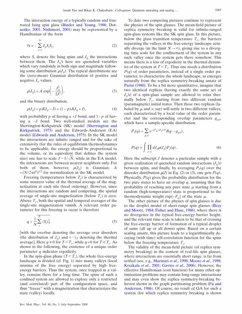
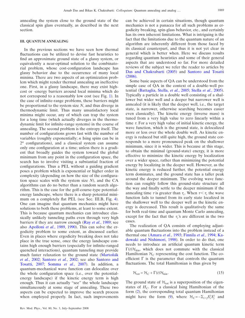
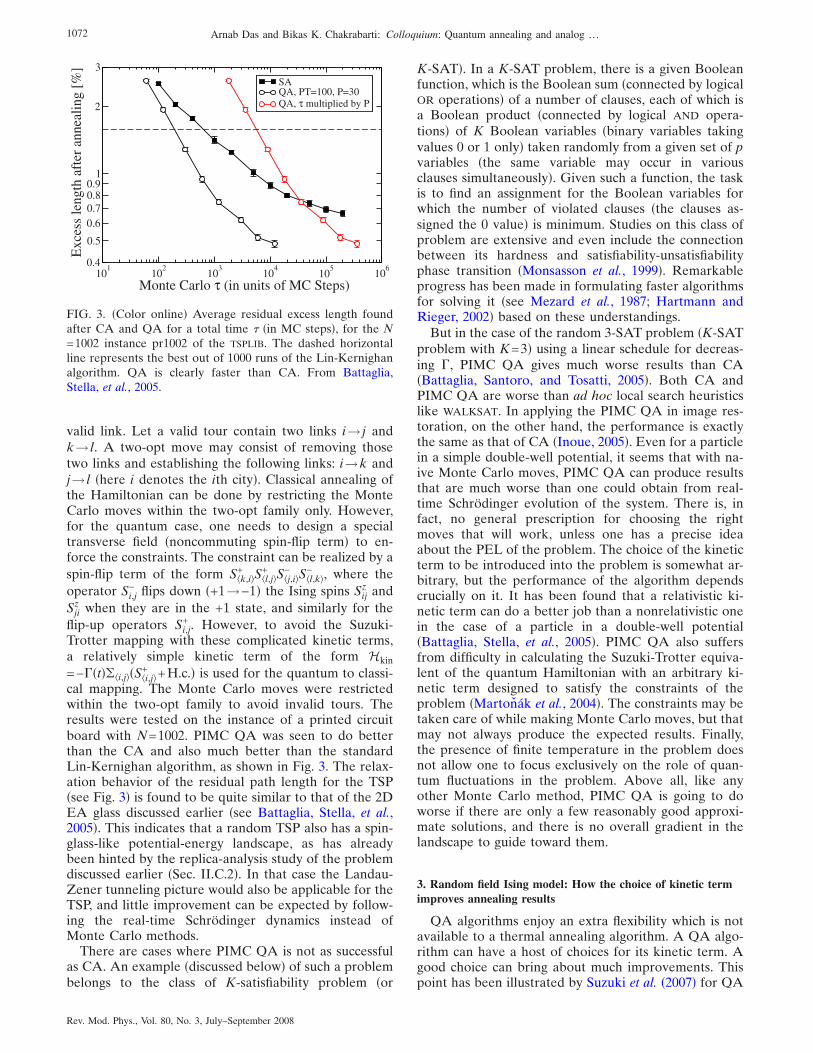
cal mapping. The Monte Carlo moves were restrictedwithin the two-opt family to avoid invalid tours. Theresults were tested on the instance of a printed circuitboard with N=1002. PIMC QA was seen to do betterthan the CA and also much better than the standardLin-Kernighan algorithm, as shown in Fig. 3. The relax-ation behavior of the residual path length for the TSP�see Fig. 3� is found to be quite similar to that of the 2DEA glass discussed earlier �see Battaglia, Stella, et al.,2005�. This indicates that a random TSP also has a spin-glass-like potential-energy landscape, as has alreadybeen hinted by the replica-analysis study of the problemdiscussed earlier �Sec. II.C.2�. In that case the Landau-Zener tunneling picture would also be applicable for theTSP, and little improvement can be expected by follow-ing the real-time Schrödinger dynamics instead ofMonte Carlo methods.

There are cases where PIMC QA is not as successfulas CA. An example �discussed below� of such a problembelongs to the class of K-satisfiability problem �or

K-SAT�. In a K-SAT problem, there is a given Booleanfunction, which is the Boolean sum �connected by logicalOR operations� of a number of clauses, each of which isa Boolean product �connected by logical AND opera-tions� of K Boolean variables �binary variables takingvalues 0 or 1 only� taken randomly from a given set of pvariables �the same variable may occur in variousclauses simultaneously�. Given such a function, the taskis to find an assignment for the Boolean variables forwhich the number of violated clauses �the clauses as-signed the 0 value� is minimum. Studies on this class ofproblem are extensive and even include the connectionbetween its hardness and satisfiability-unsatisfiabilityphase transition �Monsasson et al., 1999�. Remarkableprogress has been made in formulating faster algorithmsfor solving it �see Mezard et al., 1987; Hartmann andRieger, 2002� based on these understandings.

But in the case of the random 3-SAT problem �K-SATproblem with K=3� using a linear schedule for decreas-ing �, PIMC QA gives much worse results than CA�Battaglia, Santoro, and Tosatti, 2005�. Both CA andPIMC QA are worse than ad hoc local search heuristicslike WALKSAT. In applying the PIMC QA in image res-toration, on the other hand, the performance is exactlythe same as that of CA �Inoue, 2005�. Even for a particlein a simple double-well potential, it seems that with na-ive Monte Carlo moves, PIMC QA can produce resultsthat are much worse than one could obtain from real-time Schrödinger evolution of the system. There is, infact, no general prescription for choosing the rightmoves that will work, unless one has a precise ideaabout the PEL of the problem. The choice of the kineticterm to be introduced into the problem is somewhat ar-bitrary, but the performance of the algorithm dependscrucially on it. It has been found that a relativistic ki-netic term can do a better job than a nonrelativistic onein the case of a particle in a double-well potential�Battaglia, Stella, et al., 2005�. PIMC QA also suffersfrom difficulty in calculating the Suzuki-Trotter equiva-lent of the quantum Hamiltonian with an arbitrary ki-netic term designed to satisfy the constraints of theproblem �Martonák et al., 2004�. The constraints may betaken care of while making Monte Carlo moves, but thatmay not always produce the expected results. Finally,the presence of finite temperature in the problem doesnot allow one to focus exclusively on the role of quan-tum fluctuations in the problem. Above all, like anyother Monte Carlo method, PIMC QA is going to doworse if there are only a few reasonably good approxi-mate solutions, and there is no overall gradient in thelandscape to guide toward them.

3. Random field Ising model: How the choice of kinetic termimproves annealing results

QA algorithms enjoy an extra flexibility which is notavailable to a thermal annealing algorithm. A QA algo-rithm can have a host of choices for its kinetic term. Agood choice can bring about much improvements. Thispoint has been illustrated by Suzuki et al. �2007� for QA

��

�

�

�

��

��

��

��

101

102

103

104

105

106

Monte Carlo τ (in units of MC Steps)

0.4

0.5

0.60.70.80.9

1

2

3E

xces

sle

ngth

afte

ran

neal

ing

[%]

SAQA, PT=100, P=30

��

QA, τ multiplied by P

FIG. 3. �Color online� Average residual excess length foundafter CA and QA for a total time � �in MC steps�, for the N=1002 instance pr1002 of the TSPLIB. The dashed horizontalline represents the best out of 1000 runs of the Lin-Kernighanalgorithm. QA is clearly faster than CA. From Battaglia,Stella, et al., 2005.



of the random field Ising model, by introducing a ferro-magnetic transverse field interaction, in addition to theconventional single-spin-flip transverse field term �aspresent in the Hamiltonian �9��.

The Hamiltonian of the random-field Ising model withthe standard single-spin-flip transverse term is given by

H�t� = HC + Hkin�1� , �18�

where

HC = − J��ij

N

SizSj

z − �i=1

N

hizSi

z, �19�

hiz is the on-site random field, assuming values +1 or −1

with equal probabilities, �ij denotes the sum over near-est neighbors on a two-dimensional square lattice, and

Hkin�1� = − ��t��

i=1

n

Six. �20�

The result of QA in such a system is not satisfactorywhen J is much larger than hi

z �Sarjala et al., 2006�. If aferromagnetic transverse term of the form

Hkin�2� = − ��t��

�ij

N

SixSj

x �21�

is added to the Hamiltonian �18�, the result of QA isseen to improve considerably �Suzuki et al., 2007�. Thishappens �as indicated by exact diagonalization results onsmall systems� because the ferromagnetic transversefield term effectively increases the gap between theground state and the first excited state and thus de-creases the characteristic time scale for the system. Thisis an example of how one can utilize the flexibility inchoosing the kinetic term in QA to formulate faster al-gorithms. This also indicates how knowledge of the sys-tem’s phase diagram, the position of the quantum criticalpoint in particular �where the gap tends to vanish�, helpsin choosing additional kinetic terms and thus allows forfinding annealing paths that can avoid, to some extent,the regions of very low gap.

B. Quantum annealing using real-time adiabatic evolution

QA is basically the analog version of quantum com-putation. As for conventional analog quantum computa-tion, the hardware realization of adiabatic quantum an-nealing is rather problem specific. But once realized, itfollows the real-time Schrödinger evolution, whose exactsimulation is always intractable �the run time grows ex-ponentially with the system size� for classical computersand often also even for digital quantum computers �seeNielsen and Chuang, 2000�. The annealing behavior withthe real-time Schrödinger evolution is hence an impor-tant issue and may show features distinctly differentfrom any Monte Carlo annealing discussed so far.

The first analog algorithm was formulated by Farhiand Gutmann �1998� for solving Grover’s search prob-lem. Grover �1997� showed that a quantum-mechanical

search can reduce an O�N� classical search time toO��N� in finding a marked item from an unstructureddatabase. In the analog version, the problem was to usequantum evolution to find a given marked state amongN orthonormal states. The algorithm was formulated inthe following way. There were N mutually orthogonalnormalized states, the ith state denoted by �i . Among allof them, only one, say, the wth one, has energy E�0 andthe rest all have zero energy. Thus the state �w is“marked” energetically and the system can distinguishit. Now the question is how fast the system can evolveunder a certain Hamiltonian so that starting from anequal superposition of the N states one reaches �w . Itwas shown �Farhi and Gutmann, 1998� that if the systemevolves under a time-independent Hamiltonian of theform

Htot = E�w �w� + E�s �s� , �22�

where

�s =1

�N�i=1

N

�i , �23�

no improvement over Grover’s �N speedup is possible.Later, the problem was recast in the form of a spatialsearch �Childs and Goldstone, 2004�, where there is ad-dimensional lattice and the basis state �i is localized atthe ith lattice site. As before, the on-site potential en-ergy E is zero everywhere except at �w , where it is 1.The objective is to reach the marked state starting fromthe equal superposition of all the �i ’s. The kinetic termis formulated through the Laplacian of the lattice, whicheffectively introduces uniform hopping to all nearestneighbors from any given lattice sites, and is kept con-stant. The model is in essence an Anderson model �San-toro and Tosatti, 2006� with only a single-site disorder ofstrength O�1�. Grover’s speedup can be achieved for d�4 with such a Hamiltonian and no further improve-ment is possible. The algorithm succeeds only near thecritical value of the kinetic term �i.e., at the quantumphase transition point�. An adiabatic quantum evolutionalgorithm for Grover search was formulated in terms ofan orthonormal complete set of l-bit Ising-like basis vec-tors, where the potential energy of a given basis vector�among 2l� is 1, and for the rest it is 0. The kinetic termis the sum of all single-bit-flip terms �like the transversefield term in Eq. �9��. It connects each basis vector tothose that can be reached from it by a single-bit flip. Thekinetic term is reduced from a high value to zero follow-ing a linear schedule. A detailed analysis in light of theadiabatic theorem showed that one cannot even retrieveGrover’s speedup by sticking to the global adiabatic con-dition with fixed evolution rate as given by Eq. �16�. Thisoccurs because the minimum value of the gap varies as�min2.2−l/2 �Farhi et al., 2000�, and since the spin-flip

kinetic term is local, the numerator ��Htot˙ � of the adia-

batic factor �see Eq. �16�� is at best O�l�. However, Grov-er’s speedup can be recovered if the condition of adia-baticity is maintained locally �for more on nonlinear



annealing schedule, see also Farhi et al. �2002b� andMorita �2007�� at every instant of the evolution and therate is accelerated accordingly whenever possible �Ro-land and Cerf, 2001�. Adiabatic QA following real-timeSchrödinger evolution for satisfiability problems alsogives a different result �for smaller system size, though�compared to that obtained using PIMC QA. AdiabaticQA of an NP-complete problem, namely, the exactcover problem �as described below� has been studied forsmall systems, where a quadratic system-size depen-dence was observed �Farhi, Goldstone, Gutmann, et al.,2001�. In this problem the basis vectors are the completeset of 2l orthonormal l-bit basis vectors, denoted by��z1 �z2 ¯ �zl �; each zi is either 0 or 1. The problemconsists of a cost function HC which is the sum of manythree-bit clause functions hCl�zi ,zj ,zk�, each acting onarbitrarily chosen bits zi, zj, and zk. The clause functionis such that hCl�zi ,zj ,zk�=0 if the clause Cl is satisfied bythe states �zi , �zj , and �zk of the three bits, or elsehCl�zi ,zj ,zk�=1. The cost Hamiltonian is given by HC=�ClhCl. Thus if a basis state ��zi� dissatisfies p clauses,then HC � �zi� =p � �zi� . The question is whether there ex-ists a basis vector that satisfies all clauses for a given HC.There may be many basis vectors satisfying a clause. Allthe basis vectors will be the ground state of HC with zeroeigenvalue. If the ground state has a nonzero eigenvalue�it must be a positive integer then� then it represents thebasis with the lowest number of violated clauses, thenumber given by the eigenvalue itself. The total Hamil-tonian is given by

Htot�t� = �1 −t

�Hkin +

t

�HC, �24�

where Hkin is again the sum of all single-bit-flip opera-tors. The initial state at t=0 is taken to be the groundstate of Hkin, which is an equal superposition of all basisvectors. The system then evolves according to the time-dependent Schrödinger equation up to t=�. The valuesof � required to achieve a preassigned success probabil-ity are noted for different system sizes. The resultshowed a smooth quadratic system-size dependence forl 20 �Farhi, Goldstone, and Gutmann, 2002b�. which isquite encouraging �since it seems to give a polynomialtime solution for an NP-complete problem for small sys-tem size�, but does not really assure a quadratic behav-ior in the asymptotic �l→ � � limit.

Quadratic relaxation behavior ��res1/��, �2� wasreported by Suzuki and Okada �2005a� for real-timeadiabatic QA �employing the exact method for smallsystems and the density-matrix renormalization group�DMRG� technique for larger systems �see Suzuki andOkada, 2005b�� of a one-dimensional tight-bindingmodel with random site energies and also for a random-field Ising model on a 2D square lattice. In the first case,the kinetic term was due to hopping between nearestneighbors, while in the second case it was simply thesum of single-spin-flip operators as given by Eq. �9�.Wave-function annealing results using a similar DMRG

technique for a spin glass on a ladder have been re-ported by Rodriguez-Laguna �2007�.

It has been demonstrated that for finite-ranged sys-tems, where the interaction energy can be written as asum of interaction energies involving few variables,quantum adiabatic annealing and thermal annealingmay not differ much in efficiency. However, for prob-lems with spiky �very high but narrow� barriers in thePEL �which must include infinite-range terms in theHamiltonian, since in finite-range systems barrierheights can grow at best linearly with barrier width�,quantum annealing does much better than CA �Farhi etal., 2002a�, as argued by Ray et al. �1989�. Quantum adia-batic evolution has been employed earlier to study theSK spin glass in a transverse field; stationary character-istics over a range of the transverse field are calculatedby varying the transverse field adiabatically �Lancasterand Ritort, 1997�.

It has been argued so far that the advantage of quan-tum annealing derives mainly from the fact that quan-tum tunneling can penetrate through very high but nar-row barriers, which are hard to jump over thermally. Inthis way the cost-configuration landscapes are more ac-cessible to local moves. This is a key feature that workseven in the case of quantum Monte Carlo methods suchas PIMC QA, where one samples only a small section ofthe configuration space. However, another advantagethat quantum mechanics provides is the ability to“sense” the whole configuration space simultaneouslythrough a delocalized wave function. This sensing isgreatly handicapped by the presence of random disorderin the system, because the wave function tends to local-ize in many places, often unable to pick up the deepestwell distinctly. This feature may be utilized in searchinga golf-course-like PEL, namely, a flat landscape withvery deep and narrow wells occurring very rarely. Ifthere is only one deep well, the problem is the spatialversion of Grover’s problem. As we have seen, if thedepth � of the well is O�1� �independent of N�, then nomore than O��N� speedup can be achieved. This can beinterpreted as the inability of an exceedingly large sys-tem to sense a given small imperfection. One might wantto make the depth of the well large enough that it can-not be scaled away as the system size is increased.

We first consider the case where the well depth variesas ��N, where � is constant. For a well depth of thisorder for a spatial search at infinite dimension �the ki-netic term is infinite ranged� one gets a stunning result:The evolution time that guarantees any given probabil-ity of success becomes independent of N �Das, 2007; seeFig. 4�. However, if � scales as �N�, with ��1, thenthe speedup is lost again—a consequence of quantum-mechanical nonadiabaticity. We formulate the problemin the following way. As in the case of a spatial searchdiscussed above, we denote the state localized at the ithsite by �i . All sites except �w have zero on-site potentialenergy, while �w has an on-site potential well of depth��t�. The system is embedded in infinite dimensions andthus there is a uniform tunneling term � between any



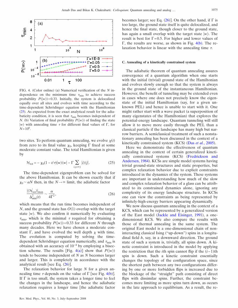
two sites. To perform quantum annealing, we evolve ��t�from zero to its final value �0, keeping � fixed at somemoderate constant value. The total Hamiltonian is givenby

Htot = − �0�1 − t/��w �w� − � �i,j;i�j

�i �j� . �25�

The time-dependent eigenproblem can be solved forthe above Hamiltonian. It can be shown exactly that if�0�N then, in the N→� limit, the adiabatic factor

��Htot˙ �max

�min2 �t�

�

4�2 , �26�

which means that the run time becomes independent ofN, and the ground state has O�1� overlap with the targetstate �w . We also confirm it numerically by evaluating�min, which is the minimal � required for obtaining asuccess probability P��w �=0.33 for different N throughmany decades. Here we have chosen a moderate con-stant �, and have evolved the well depth � with time.The evolution is computed by solving the time-dependent Schrödinger equation numerically, and �min isobtained with an accuracy of 10−4 by employing a bisec-tion scheme. The results �Fig. 4�a�� show that P��w �tends to become independent of N as N becomes largerand larger. This is completely in accordance with theanalytical result �see Eq. �26��.

The relaxation behavior for large N for a given an-nealing time � depends on the value of � �see Fig. 4�b��.If � is too small, the system takes a longer time to feelthe changes in the landscape, and hence the adiabaticrelaxation requires a longer time �the adiabatic factor

becomes larger; see Eq. �26��. On the other hand, if � istoo large, the ground state itself is quite delocalized, andhence the final state, though closer to the ground state,has again a small overlap with the target state �w . Theresult is best for �=0.5. For higher and lower values of�, the results are worse, as shown in Fig. 4�b�. The re-laxation behavior is linear with the annealing time �.

C. Annealing of a kinetically constrained system

The adiabatic theorem of quantum annealing assuresconvergence of a quantum algorithm when one startswith the initial �trivial� ground state of the Hamiltonianand evolves slowly enough so that the system is alwaysin the ground state of the instantaneous Hamiltonian.However, the benefit of tunneling may be extended evenin cases where one does not precisely know the eigen-state of the initial Hamiltonian �say, for a given un-known PEL� and hence is unable to start with it. Onemight rather start with a wave packet �a superposition ofmany eigenstates of the Hamiltonian� that explores thepotential-energy landscape. Quantum tunneling will stillallow it to move more easily through the PEL than aclassical particle if the landscape has many high but nar-row barriers. A semiclassical treatment of such a nonsta-tionary annealing has been discussed in the context of akinetically constrained system �KCS� �Das et al., 2005�.

Here we demonstrate the effectiveness of quantumannealing in the context of certain generalized kineti-cally constrained systems �KCS� �Fredrickson andAndersen, 1984�. KCSs are simple model systems havingtrivial ground-state structures and static properties, butcomplex relaxation behavior due to explicit constraintsintroduced in the dynamics of the system. These systemsare important in understanding how much of the slowand complex relaxation behavior of a glass can be attrib-uted to its constrained dynamics alone, ignoring anycomplexity of its energy landscape structure. In KCSsone can view the constraints as being represented byinfinitely-high-energy barriers appearing dynamically.

We now discuss quantum annealing in the context of aKCS, which can be represented by a generalized versionof the East model �Jackle and Eisinger, 1991�, a one-dimensional KCS. We also compare the results withthose of thermal annealing in the same system. Theoriginal East model is a one-dimensional chain of non-interacting classical Ising �“up-down”� spins in a longitu-dinal field h, say, in a downward direction. The groundstate of such a system is, trivially, all spins down. A ki-netic constraint is introduced in the model by applyingthe restriction that the ith spin cannot flip if the �i−1�thspin is down. Such a kinetic constraint essentiallychanges the topology of the configuration space, sincethe shortest path between any two configurations differ-ing by one or more forbidden flips is increased due tothe blockage of the “straight” path consisting of directflips with dissimilar spins. Further, the constraint be-comes more limiting as more spins turn down, as occursin the late approach to equilibrium. As a result, the re-

FIG. 4. �Color online� �a� Numerical verification of the N in-dependence on the minimum time �min to achieve successprobability P��w �=0.33. Initially, the system is delocalizedequally over all sites and evolves with time according to thetime-dependent Schrödinger equation with the Hamiltonian�25�. As expected from the exact analytical result for the adia-baticity condition, it is seen that �min becomes independent ofN. �b� Variation of final probability P��w � of finding the state�w with annealing time � for different final values of �, forN=106.



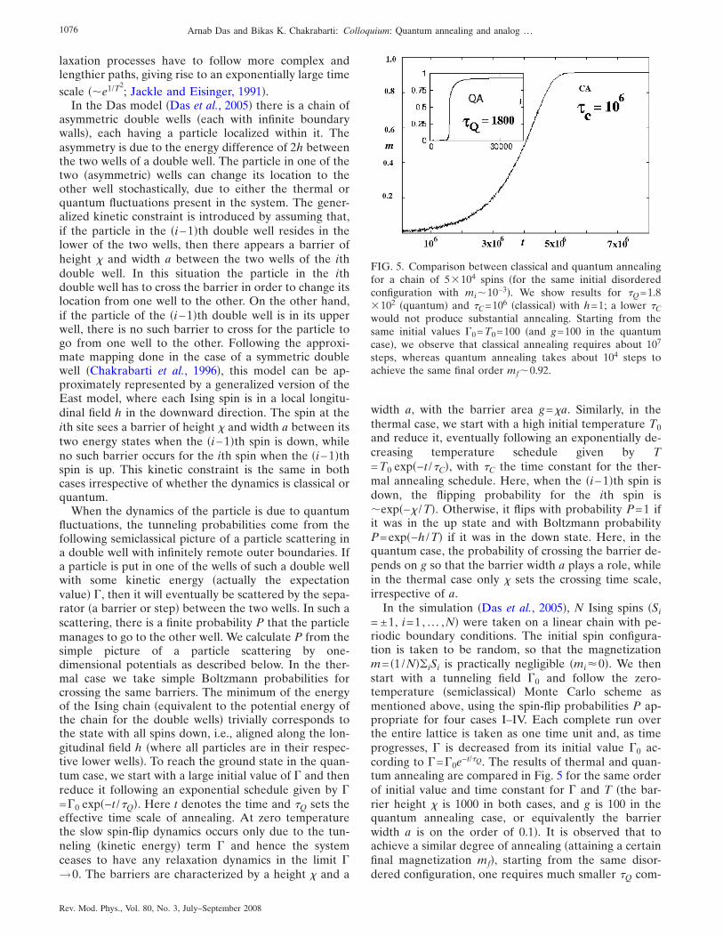
laxation processes have to follow more complex andlengthier paths, giving rise to an exponentially large timescale �e1/T2

; Jackle and Eisinger, 1991�.In the Das model �Das et al., 2005� there is a chain of

asymmetric double wells �each with infinite boundarywalls�, each having a particle localized within it. Theasymmetry is due to the energy difference of 2h betweenthe two wells of a double well. The particle in one of thetwo �asymmetric� wells can change its location to theother well stochastically, due to either the thermal orquantum fluctuations present in the system. The gener-alized kinetic constraint is introduced by assuming that,if the particle in the �i−1�th double well resides in thelower of the two wells, then there appears a barrier ofheight � and width a between the two wells of the ithdouble well. In this situation the particle in the ithdouble well has to cross the barrier in order to change itslocation from one well to the other. On the other hand,if the particle of the �i−1�th double well is in its upperwell, there is no such barrier to cross for the particle togo from one well to the other. Following the approxi-mate mapping done in the case of a symmetric doublewell �Chakrabarti et al., 1996�, this model can be ap-proximately represented by a generalized version of theEast model, where each Ising spin is in a local longitu-dinal field h in the downward direction. The spin at theith site sees a barrier of height � and width a between itstwo energy states when the �i−1�th spin is down, whileno such barrier occurs for the ith spin when the �i−1�thspin is up. This kinetic constraint is the same in bothcases irrespective of whether the dynamics is classical orquantum.

When the dynamics of the particle is due to quantumfluctuations, the tunneling probabilities come from thefollowing semiclassical picture of a particle scattering ina double well with infinitely remote outer boundaries. Ifa particle is put in one of the wells of such a double wellwith some kinetic energy �actually the expectationvalue� �, then it will eventually be scattered by the sepa-rator �a barrier or step� between the two wells. In such ascattering, there is a finite probability P that the particlemanages to go to the other well. We calculate P from thesimple picture of a particle scattering by one-dimensional potentials as described below. In the ther-mal case we take simple Boltzmann probabilities forcrossing the same barriers. The minimum of the energyof the Ising chain �equivalent to the potential energy ofthe chain for the double wells� trivially corresponds tothe state with all spins down, i.e., aligned along the lon-gitudinal field h �where all particles are in their respec-tive lower wells�. To reach the ground state in the quan-tum case, we start with a large initial value of � and thenreduce it following an exponential schedule given by �=�0 exp�−t /�Q�. Here t denotes the time and �Q sets theeffective time scale of annealing. At zero temperaturethe slow spin-flip dynamics occurs only due to the tun-neling �kinetic energy� term � and hence the systemceases to have any relaxation dynamics in the limit �→0. The barriers are characterized by a height � and a

width a, with the barrier area g=�a. Similarly, in thethermal case, we start with a high initial temperature T0and reduce it, eventually following an exponentially de-creasing temperature schedule given by T=T0 exp�−t /�C�, with �C the time constant for the ther-mal annealing schedule. Here, when the �i−1�th spin isdown, the flipping probability for the ith spin isexp�−� /T�. Otherwise, it flips with probability P=1 ifit was in the up state and with Boltzmann probabilityP=exp�−h /T� if it was in the down state. Here, in thequantum case, the probability of crossing the barrier de-pends on g so that the barrier width a plays a role, whilein the thermal case only � sets the crossing time scale,irrespective of a.

In the simulation �Das et al., 2005�, N Ising spins �Si= ±1, i=1, . . . ,N� were taken on a linear chain with pe-riodic boundary conditions. The initial spin configura-tion is taken to be random, so that the magnetizationm= �1/N��iSi is practically negligible �mi�0�. We thenstart with a tunneling field �0 and follow the zero-temperature �semiclassical� Monte Carlo scheme asmentioned above, using the spin-flip probabilities P ap-propriate for four cases I–IV. Each complete run overthe entire lattice is taken as one time unit and, as timeprogresses, � is decreased from its initial value �0 ac-cording to �=�0e−t/�Q. The results of thermal and quan-tum annealing are compared in Fig. 5 for the same orderof initial value and time constant for � and T �the bar-rier height � is 1000 in both cases, and g is 100 in thequantum annealing case, or equivalently the barrierwidth a is on the order of 0.1�. It is observed that toachieve a similar degree of annealing �attaining a certainfinal magnetization mf�, starting from the same disor-dered configuration, one requires much smaller �Q com-

FIG. 5. Comparison between classical and quantum annealingfor a chain of 5�104 spins �for the same initial disorderedconfiguration with mi10−3�. We show results for �Q=1.8�102 �quantum� and �C=106 �classical� with h=1; a lower �Cwould not produce substantial annealing. Starting from thesame initial values �0=T0=100 �and g=100 in the quantumcase�, we observe that classical annealing requires about 107

steps, whereas quantum annealing takes about 104 steps toachieve the same final order mf0.92.



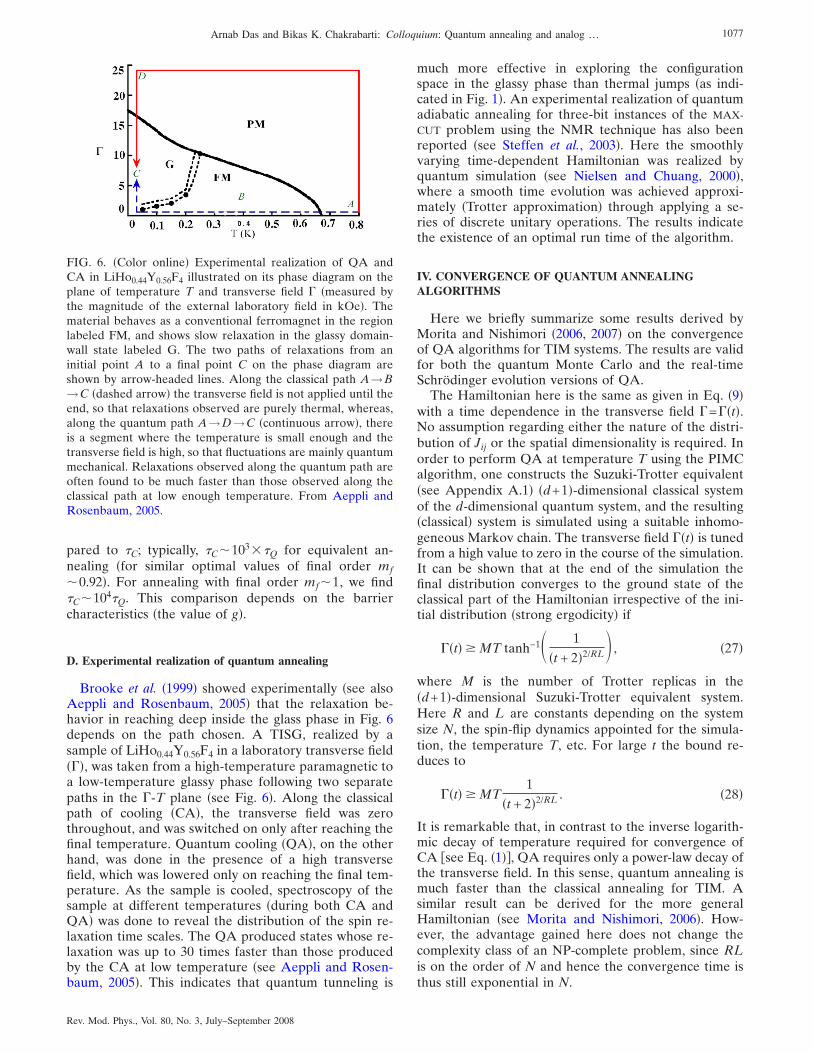
pared to �C; typically, �C103��Q for equivalent an-nealing �for similar optimal values of final order mf0.92�. For annealing with final order mf1, we find�C104�Q. This comparison depends on the barriercharacteristics �the value of g�.

D. Experimental realization of quantum annealing

Brooke et al. �1999� showed experimentally �see alsoAeppli and Rosenbaum, 2005� that the relaxation be-havior in reaching deep inside the glass phase in Fig. 6depends on the path chosen. A TISG, realized by asample of LiHo0.44Y0.56F4 in a laboratory transverse field��, was taken from a high-temperature paramagnetic toa low-temperature glassy phase following two separatepaths in the �-T plane �see Fig. 6�. Along the classicalpath of cooling �CA�, the transverse field was zerothroughout, and was switched on only after reaching thefinal temperature. Quantum cooling �QA�, on the otherhand, was done in the presence of a high transversefield, which was lowered only on reaching the final tem-perature. As the sample is cooled, spectroscopy of thesample at different temperatures �during both CA andQA� was done to reveal the distribution of the spin re-laxation time scales. The QA produced states whose re-laxation was up to 30 times faster than those producedby the CA at low temperature �see Aeppli and Rosen-baum, 2005�. This indicates that quantum tunneling is

much more effective in exploring the configurationspace in the glassy phase than thermal jumps �as indi-cated in Fig. 1�. An experimental realization of quantumadiabatic annealing for three-bit instances of the MAX-CUT problem using the NMR technique has also beenreported �see Steffen et al., 2003�. Here the smoothlyvarying time-dependent Hamiltonian was realized byquantum simulation �see Nielsen and Chuang, 2000�,where a smooth time evolution was achieved approxi-mately �Trotter approximation� through applying a se-ries of discrete unitary operations. The results indicatethe existence of an optimal run time of the algorithm.

IV. CONVERGENCE OF QUANTUM ANNEALINGALGORITHMS

Here we briefly summarize some results derived byMorita and Nishimori �2006, 2007� on the convergenceof QA algorithms for TIM systems. The results are validfor both the quantum Monte Carlo and the real-timeSchrödinger evolution versions of QA.

The Hamiltonian here is the same as given in Eq. �9�with a time dependence in the transverse field �=��t�.No assumption regarding either the nature of the distri-bution of Jij or the spatial dimensionality is required. Inorder to perform QA at temperature T using the PIMCalgorithm, one constructs the Suzuki-Trotter equivalent�see Appendix A.1� �d+1�-dimensional classical systemof the d-dimensional quantum system, and the resulting�classical� system is simulated using a suitable inhomo-geneous Markov chain. The transverse field ��t� is tunedfrom a high value to zero in the course of the simulation.It can be shown that at the end of the simulation thefinal distribution converges to the ground state of theclassical part of the Hamiltonian irrespective of the ini-tial distribution �strong ergodicity� if

��t� � MT tanh−1� 1

�t + 2�2/RL , �27�

where M is the number of Trotter replicas in the�d+1�-dimensional Suzuki-Trotter equivalent system.Here R and L are constants depending on the systemsize N, the spin-flip dynamics appointed for the simula-tion, the temperature T, etc. For large t the bound re-duces to

��t� � MT1

�t + 2�2/RL . �28�

It is remarkable that, in contrast to the inverse logarith-mic decay of temperature required for convergence ofCA �see Eq. �1��, QA requires only a power-law decay ofthe transverse field. In this sense, quantum annealing ismuch faster than the classical annealing for TIM. Asimilar result can be derived for the more generalHamiltonian �see Morita and Nishimori, 2006�. How-ever, the advantage gained here does not change thecomplexity class of an NP-complete problem, since RLis on the order of N and hence the convergence time isthus still exponential in N.

FIG. 6. �Color online� Experimental realization of QA andCA in LiHo0.44Y0.56F4 illustrated on its phase diagram on theplane of temperature T and transverse field � �measured bythe magnitude of the external laboratory field in kOe�. Thematerial behaves as a conventional ferromagnet in the regionlabeled FM, and shows slow relaxation in the glassy domain-wall state labeled G. The two paths of relaxations from aninitial point A to a final point C on the phase diagram areshown by arrow-headed lines. Along the classical path A→B→C �dashed arrow� the transverse field is not applied until theend, so that relaxations observed are purely thermal, whereas,along the quantum path A→D→C �continuous arrow�, thereis a segment where the temperature is small enough and thetransverse field is high, so that fluctuations are mainly quantummechanical. Relaxations observed along the quantum path areoften found to be much faster than those observed along theclassical path at low enough temperature. From Aeppli andRosenbaum, 2005.



For real-time Schrödinger dynamics at T=0, thebound for the decay of the transverse field is again of theform

��t� � ��t�−1/�2N−1�, �29�

where � is exponentially small in N for large N. Al-though the dynamics of PIMC QA and real-timeSchrödinger evolution are completely different, thepower-law bound on the annealing schedule is strikinglysimilar.

V. QUANTUM QUENCHING

Instead of annealing, one can quench a system by re-ducing the transverse field from �i ��c� to �f ��c� andfollow the relaxation dynamics after that. Here �c de-notes the quantum critical point for the system. This canhelp to prepare a state of the system with substantialorder in a short time. Recently, quantum quenching dy-namics in different systems, in particular for suddenquenching across a quantum critical point, have beenstudied extensively �Sengupta et al., 2004; Calabrese andCardy, 2006; Das et al., 2006; Mukherjee et al., 2007; Sen-gupta et al., 2008�. The �exact� results for the after-quench dynamics, following a sudden quench of aninfinite-range Ising model in transverse field �Das et al.,2006, see Appendix B�, are shown in Fig. 7. The resultsindicate that for a purely quantum system �small S�, onemight reach a nonstationary oscillatory state with a sub-stantial value for the long-time average �over the largesttime scale� of order ��Si

z�2�t� if the quenching is donefrom �i��c to �f=�c /2. Thus one gets a state �thoughnonstationary� which has considerable order, in just one-step quenching. However, if the quenching is carried out

with a high but finite rate, one ends up reaching an ex-cited state with topological defects �see Kibble, 1976;Zurek, 1985; Sengupta et al., 2008�.

VI. SUMMARY AND DISCUSSIONS

Unlike gate-based quantum computers �see, e.g., Ek-ert and Jozsa, 1996; Nielsen and Chuang, 2000; Galindoand Martin-Delgado, 2002�, annealing of a physical sys-tem toward the optimal state �encoded in the groundstate of the final Hamiltonian� in the classical limit natu-rally achieves analog quantum computation. As dis-cussed here, utilization of quantum-mechanical tunnel-ing through classically localized states in annealing ofglasses has opened up this new paradigm for analogquantum computation of hard optimization problemsthrough adiabatic reduction of quantum fluctuations.

We reviewed the recent success in annealing, or opti-mizing, the cost functions of complex systems, utilizingquantum fluctuations rather than thermal fluctuations�see Santoro and Tosatti, 2006, for a more technical re-view�. As mentioned, following the early indication byRay et al. �1989� and the pioneering demonstrations,theoretically by Amara et al. �1993�, Finnila et al. �1994�,Kadowaki and Nishimori �1998�, Farhi, Goldstone, Gut-mann, et al. �2001�, and Santoro et al. �2002�, and experi-mentally by Brooke et al. �1999�, the quantum annealingtechnique has now emerged as a successful technique foroptimization of complex cost functions. The literatureexploring its success and also its limitations is also con-siderably developed at present.

These concepts are introduced through discussions onthe mapping of such hard problems to classical spin-glass problems, discussions on quantum spin glasses, andconsequent annealing. The physics of classical spinglasses �see Sec. II� offers us knowledge of the energy orthe thermodynamic potential and their landscape struc-tures. Mapping of computationally hard problems likethe TSP, etc., to their corresponding classical spin-glassmodels also helped in understanding their complexity�Sec. II.C�. The time scale for tunneling through an en-ergy barrier quantum mechanically involves not only theheight of the barrier, but also its width; the narrower thebarrier, the faster the tunneling �for constant height�.Thermal fluctuations, on the other hand, see only thebarrier height. This reduction of tunneling time with bar-rier width helps in relaxing a quantum system muchfaster in some cases. This leads to quantum annealing, aframework for constructing general heuristics to find ap-proximate solutions of hard optimization problems.While simulated annealing employs the strategy of slowcooling, physical or in simulations, to find the groundstate of glassy systems, quantum annealing employsquantum fluctuations �see Sec. III�. As mentioned, thiseffectively reduces Planck’s constant to zero in order toreach the classically optimized �minimum cost� state.This reduction, when done completely adiabatically,guarantees that the system will be found in the groundstate of the classical glass at the end �provided there isno crossing of energy levels with the ground state in the

FIG. 7. �Color online� Long-time average �see Appendix A�O= ��Stot

z �2 as a function of �f /J for different S. The solid,dotted, dash-dotted, and dashed lines represent, respectively,the results for S=50, 100, 200, and 500. O peaks around �f /J=0.25 and the peak value decreases with increasing S. For allplots we have chosen �i /J=2. From Das et al., 2006.



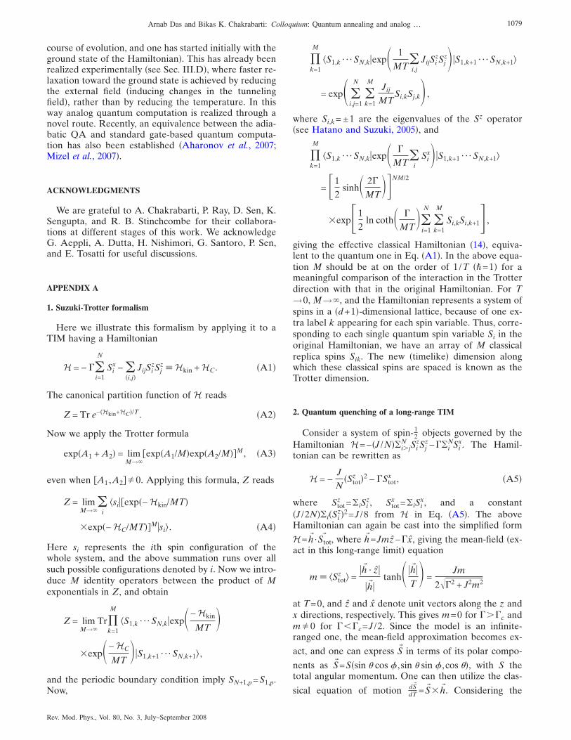
course of evolution, and one has started initially with theground state of the Hamiltonian�. This has already beenrealized experimentally �see Sec. III.D�, where faster re-laxation toward the ground state is achieved by reducingthe external field �inducing changes in the tunnelingfield�, rather than by reducing the temperature. In thisway analog quantum computation is realized through anovel route. Recently, an equivalence between the adia-batic QA and standard gate-based quantum computa-tion has also been established �Aharonov et al., 2007;Mizel et al., 2007�.

ACKNOWLEDGMENTS

We are grateful to A. Chakrabarti, P. Ray, D. Sen, K.Sengupta, and R. B. Stinchcombe for their collabora-tions at different stages of this work. We acknowledgeG. Aeppli, A. Dutta, H. Nishimori, G. Santoro, P. Sen,and E. Tosatti for useful discussions.

APPENDIX A

1. Suzuki-Trotter formalism

Here we illustrate this formalism by applying it to aTIM having a Hamiltonian

H = − ��i=1

N

Six − �

�i,j�JijSi

zSjz � Hkin + HC. �A1�

The canonical partition function of H reads

Z = Tr e−�Hkin+HC�/T. �A2�

Now we apply the Trotter formula

exp�A1 + A2� = limM→�

�exp�A1/M�exp�A2/M��M, �A3�

even when �A1 ,A2��0. Applying this formula, Z reads

Z = limM→�

�i

�si��exp�− Hkin/MT�

�exp�− HC/MT��M�si . �A4�

Here si represents the ith spin configuration of thewhole system, and the above summation runs over allsuch possible configurations denoted by i. Now we intro-duce M identity operators between the product of Mexponentials in Z, and obtain

Z = limM→�

Tr�k=1

M

�S1,k ¯ SN,k�exp�− Hkin

MT

�exp�− HC

MT�S1,k+1 ¯ SN,k+1 ,

and the periodic boundary condition imply SN+1,p=S1,p.Now,

�k=1

M

�S1,k ¯ SN,k�exp� 1

MT�i,j

JijSizSj

z�S1,k+1 ¯ SN,k+1

= exp��i,j=1

N

�k=1

MJij

MTSi,kSj,k ,

where Si,k= ±1 are the eigenvalues of the Sz operator�see Hatano and Suzuki, 2005�, and

�k=1

M

�S1,k ¯ SN,k�exp� �

MT�i

Six�S1,k+1 ¯ SN,k+1

= �12

sinh� 2�

MT�NM/2

�exp�12

ln coth� �

MT�

i=1

N

�k=1

M

Si,kSi,k+1� ,

giving the effective classical Hamiltonian �14�, equiva-lent to the quantum one in Eq. �A1�. In the above equa-tion M should be at on the order of 1/T ��=1� for ameaningful comparison of the interaction in the Trotterdirection with that in the original Hamiltonian. For T→0, M→�, and the Hamiltonian represents a system ofspins in a �d+1�-dimensional lattice, because of one ex-tra label k appearing for each spin variable. Thus, corre-sponding to each single quantum spin variable Si in theoriginal Hamiltonian, we have an array of M classicalreplica spins Sik. The new �timelike� dimension alongwhich these classical spins are spaced is known as theTrotter dimension.

2. Quantum quenching of a long-range TIM

Consider a system of spin-12 objects governed by the

Hamiltonian H=−�J /N��i�jN Si

zSjz−��i

NSix. The Hamil-

tonian can be rewritten as

H = −J

N�Stot

z �2 − �Stotx , �A5�

where Stotz =�iSi

z, Stotx =�iSi

x, and a constant�J /2N��i�Si

z�2=J /8 from H in Eq. �A5�. The aboveHamiltonian can again be cast into the simplified form

H=h� ·Stot� , where h� =Jmz−�x, giving the mean-field �ex-

act in this long-range limit� equation

m � �Stotz =

�h� · z�

�h� �tanh� �h� �

T =

Jm

2��2 + J2m2

at T=0, and z and x denote unit vectors along the z andx directions, respectively. This gives m=0 for ��c andm�0 for ��c=J /2. Since the model is an infinite-ranged one, the mean-field approximation becomes ex-

act, and one can express S� in terms of its polar compo-

nents as S� =S�sin � cos � , sin � sin � , cos ��, with S thetotal angular momentum. One can then utilize the clas-

sical equation of motion dS�

dT =S� �h� . Considering the



above equation for the z and x components, we get

d�

dt= � sin � and

d�

dt= −

J

2cos � + � cot � cos � .

�A6�

Here we have S=N /2. If the system is now quenchedfrom above its quantum critical point ��c finally to�f��c, then one can write �see Das et al., 2006�, equat-ing the energies of the states with and without any order,respectively, �f= �J /4�cos2�+�f sin � cos �. Using this,one gets from Eq. �A6�

d�

dt=

��f2 sin2� − ��f − �J/4�cos2��2

sin �� f�� . �A7�

This has zeros �turning points� at �1=sin−1��1−4�f /J � �and �2=� /2. One can therefore obtain��Stot

z �2 = �cos2� =N /D, where N=��1

�2d� cos2� / f��=4�8�f�J−2�f� /J and D=��1

�2d� / f��, giving the behaviorshown in Fig. 7.

REFERENCES

Aeppli, G., and T. F. Rosenbaum, 2005, in Quantum Annealingand Related Optimization Methods, edited by A. Das and B.K. Chakrabarti, Lecture Notes in Physics No. 679 �Springer-Verlag, Heidelberg�, pp. 159–169.

Aharonov, D., W. van Dam, J. Kempe, Z. Landau, S. Lloyd,and O. Regev, 2007, SIAM J. Comput. 37 166.

Alvarez, J. A., and F. Ritort, 1996, J. Phys. A 29, 7355.Amara, P., D. Hsu, and J. E. Straub, 1993, J. Phys. Chem. 97,

6715.Apolloni, B., C. Carvalho, and D. de Falco, 1989, Stochastic

Proc. Appl. 33, 233.Apolloni, B., N. Cesa-Bianchi, and D. de Falco, 1990, in Sto-

chastic Processes, Physics and Geometry, edited by S. Albev-erio et al. �World Scientific, Singapore�, p. 97.

Barahona, F., 1982, J. Phys. A 15, 3241.Battaglia, D. A., G. E. Santoro, and E. Tosatti, 2005, Phys.

Rev. E 71, 066707.Battaglia, D. A., L. Stella, O. Zagordi, G. E. Santoro, and E.

Tosatti, 2005, in Quantum Annealing and Related Optimiza-tion Methods, edited by A. Das and B. K. Chakrabarti, Lec-ture Notes in Physics No. 679 �Springer-Verlag, Heidelberg�,pp. 171–204.

Bearwood, J., J. H. Halton, and J. H. Hammersley, 1959, Proc.Cambridge Philos. Soc. 55, 299.

Bhatt, R. N., 1998, in Spin Glasses and Random Fields, editedby A. P. Young �World Scientific, Singapore�, pp. 225–249.

Binder, K., and A. P. Young, 1986, Rev. Mod. Phys. 58, 801.Bray, A. J., and M. A. Moore, 1984, J. Phys. C 17, L463.Brooke, J., D. Bitko, T. F. Rosenbaum, and G. Aeppli, 1999,

Science 284, 779.Brooke, J., T. F. Rosenbaum, and G. Aeppli, 2001, Nature

�London� 413, 610.Calabrese, P., and J. Cardy, 2006, Phys. Rev. Lett. 96, 136801.Chakrabarti, B. K., 1981, Phys. Rev. B 24, 4062.Chakrabarti, B. K., A. Dutta, and P. Sen, 1996, Quantum Ising

Phases and Transitions in Transverse Ising Models �Springer-Verlag, Heidelberg�.

Chakraborti, A., and B. K. Chakrabarti, 2000, Eur. Phys. J. B

16, 667.Childs, A. M., and J. Goldstone, 2004, Phys. Rev. A 70, 022314.Das, A., 2007, unpublished �see also Ph.D. thesis, Jadavpur

University, Kolkata, 2008�.Das, A., and B. K. Chakrabarti, 2005, Eds., Quantum Anneal-

ing and Related Optimization Methods, Lecture Notes inPhysics No. 679 �Springer-Verlag, Heidelberg�.

Das, A., B. K. Chakrabarti, and R. B. Stinchcombe, 2005,Phys. Rev. E 72, 026701.

Das, A., K. Sengupta, D. Sen, and B. K. Chakrabarti, 2006,Phys. Rev. B 74, 144423.

Dotsenko, V., 2001, Introduction to the Replica Theory of Dis-ordered Statistical Systems �Cambridge University Press,Cambridge, UK�.

Edwards, S. F., and P. W. Anderson, 1975, J. Phys. F: Met.Phys. 5, 965.

Ekert, A., and R. Jozsa, 1996, Rev. Mod. Phys. 68, 733.Farhi, E., J. Goldstone, and S. Gutmann, 2002a, e-print

arXiv:quant-ph/0201031.Farhi, E., J. Goldstone, and S. Gutmann, 2002b, e-print

arXiv:quant-ph/0208135.Farhi, E., J. Goldstone, S. Gutmann, J. Lapan, A. Ludgren,

and D. Preda, 2001, Science 292, 472.Farhi, E., J. Goldstone, S. Gutmann, and M. Sipser, 2000,

e-print arXiv:quant-ph/0001106.Farhi, E., and S. Gutmann, 1998, Phys. Rev. A 57, 2403.Finnila, A. B., M. A. Gomez, C. Sebenik, C. Stenson, and D. J.

Doll, 1994, Chem. Phys. Lett. 219, 343.Fisher, D. S., and D. A. Huse, 1986, Phys. Rev. Lett. 56, 1601.Fredrickson, G. H., and H. C. Andersen, 1984, Phys. Rev. Lett.

53, 1244.Fu, Y., and P. W. Anderson, 1986, J. Phys. A 19, 1620.Galindo, A., and M. A. Martin-Delgado, 2002, Rev. Mod.

Phys. 74, 347.Garey, M. R., and D. S. Johnson, 1979, Computers and Intrac-

tability: Guide to the Theory of NP-Completeness �Freeman,San Francisco�.

Gaviro, P. S., J. J. Ruiz-Lorenzo, and A. Tarancon, 2006, J.Phys. A 39, 8567.

Geman, S., and D. Geman, 1984, IEEE Trans. Pattern Anal.Mach. Intell. 6, 721.

Goldschmidt, Y. Y., and P.-Y. Lai, 1990, Phys. Rev. Lett. 64,2467.

Grover, L. K., 1997, Phys. Rev. Lett. 79, 325.Guo, M., R. N. Bhatt, and D. A. Huse, 1994, Phys. Rev. Lett.

72, 4137.Hartmann, A., and H. Rieger, 2002, Optimization in Physics

�Wiley VCH, Darmstadt�.Hatano, N., and M. Suzuki, 2005, in Quantum Annealing and

Related Optimization Methods, edited by A. Das and B. K.Chakrabarti, Lecture Notes in Physics No. 679 �Springer-Verlag, Heidelberg�, pp. 37–67.

Huse, D. A., and D. S. Fisher, 1986, Phys. Rev. Lett. 57, 2203.Inoue, J.-I., 2005, in Quantum Annealing and Related Optimi-

zation Methods, edited by A. Das and B. K. Chakrabarti,Lecture Notes in Physics No. 679 �Springer-Verlag, Heidel-berg�, pp. 259–296.

Ishii, H., and T. Yamamoto, 1985, J. Phys. C 18, 6225.Jackle, J., and S. Eisinger, 1991, Z. Phys. B: Condens. Matter

84, 115.Kadowaki, T., and H. Nishimori, 1998, Phys. Rev. E 58, 5355.Kibble, T. W. B., 1976, J. Phys. A 9, 1387.Kim, D.-H., and J.-J. Kim, 2002, Phys. Rev. B 66, 054432.



Kirkpatrick, S., C. D. Gelatt, and M. P. Vecchi, 1983, Science220, 671.

Krzakala, F., J. Houdayer, E. Marinari, O. C. Martin, and G.Parisi, 2001, Phys. Rev. Lett. 87, 197204.

Lancaster, D., and F. Ritort, 1997, J. Phys. A 30, L41.Marinari, E., G. Parisi, J. J. Ruiz-Lorenzo, and F. Zuliani, 1998,

Phys. Rev. Lett. 82, 5176.Martonák, R., G. E. Santoro, and E. Tosatti, 2002, Phys. Rev.

B 66, 094203.Martonák, R., G. E. Santoro, and E. Tosatti, 2004, Phys. Rev.

E 70, 057701.Mezard, M., G. Parisi, and M. A. Virasoro, 1987, Spin Glass

Theory and Beyond, Lecture Note in Physics No. 9 �WorldScientific, Singapore�, and references therein.

Miller, J., and D. A. Huse, 1993, Phys. Rev. Lett. 70, 3147.Mizel, A., D. A. Lidar, and M. Mitchell, 2007, Phys. Rev. Lett.

99, 070502.Monasson, R., R. Zecchina, S. Kirkpatrick, B. Selman, and L.

Troyansky, 1999, Nature �London� 400, 133.Moore, M. A., H. Bokil, and B. Drossel, 1998, Phys. Rev. Lett.

81, 4252.Morita, S., 2007, J. Phys. Soc. Jpn. 76, 104001.Morita, S., and H. Nishimori, 2006, J. Phys. A 39, 13903.Morita, S., and H. Nishimori, 2007, J. Phys. Soc. Jpn. 76,

064002.Mukherjee, V., U. Divakaran, A. Dutta, and D. Sen, 2007,

Phys. Rev. B 76, 174303.Nielsen, M. A., and I. L. Chuang, 2000, Quantum Computation

and Quantum Information �Cambridge University Press,Cambridge, UK�.

Nishimori, H., 2001, Statistical Physics of Spin Glasses and In-formation Processing: An Introduction �Oxford UniversityPress, Oxford�.

Papadimitriou, C. H., and K. Steiglitz, 1998, CombinatorialOptimization: Algorithm and Complexity �Dover, New York�.

Parisi, G., 1980, J. Phys. A 13, 1101.Percus, A., and O. C. Martin, 1996, Phys. Rev. Lett. 76, 1188.Ray, P., B. K. Chakrabarti, and A. Chakrabarti, 1989, Phys.

Rev. B 39, 11828.Rieger, H., 2005, in Quantum Annealing and Related Optimi-

zation Methods, edited by A. Das and B. K. Chakrabarti,Lecture Notes in Physics No. 679 �Springer-Verlag, Heidel-berg�, pp. 69–97.

Roland, J., and N. J. Cerf, 2001, Phys. Rev. A 65, 042308.

Rodriguez-Laguna, J., 2007, J. Stat. Mech.: Theory Exp. 2007,P05008.

Sachdev, S., 1999, Quantum Phase Transitions �CambridgeUniversity Press, Cambridge, UK�.

Santoro, G. E., R. Martonák, E. Tosatti, and R. Car, 2002,Science 295, 2427.

Santoro, G. E., and E. Tosatti, 2006, J. Phys. A 39, R393.Santoro, G. E., and E. Tosatti, 2007, Nat. Phys. 3, 593.Sarandy, M. S., L.-A. Wu, and D. A. Lidar, 2004, Quantum Inf.

Process. 3, 331.Sarjala, M., V. Petäjä, and M. Alava, 2006, J. Stat. Mech.:

Theory Exp. 2006, PO 1008.Sengupta, K., S. Powell, and S. Sachdev, 2004, Phys. Rev. A 69,

053616.Sengupta, K., D. Sen, and S. Mondal, 2008, Phys. Rev. Lett.

100, 077204.Sherrington, D., and S. Kirkpatrick, 1975, Phys. Rev. Lett. 35,

1792.Schechter, M., and N. Laflorencie, 2006, Phys. Rev. Lett. 97,

137204.Silevitch, D. M., D. Bitko, J. Brooke, S. Ghosh, G. Aeppli, and

T. F. Rosenbaum, 2007, Nature �London� 448, 567.Somma, R. D., C. D. Batista, and G. Ortiz, 2007, Phys. Rev.

Lett. 99, 030603.Suzuki, S., H. Nishimori, and M. Suzuki, 2007, Phys. Rev. E 75,

051112.Suzuki, S., and M. Okada, 2005a, J. Phys. Soc. Jpn. 74, 1649.Suzuki, S., and M. Okada, 2005b, in Quantum Annealing and

Related Optimization Methods, edited by A. Das and B. K.Chakrabarti, Lecture Notes in Physics No. 679 �Springer-Verlag, Heidelberg�.

Steffen, M., v. W. Dam, T. Hogg, G. Breyta, and I. Chuang,2003, Phys. Rev. Lett. 90, 067903.

Stella, L., G. Santoro, and E. A. Tosatti, 2005, Phys. Rev. B 72,014303.

Thirumalai, D., Q. Li, and T. R. Kirkpatrick, 1989, J. Phys. A22, 2339.

Wu, W., D. Bitko, T. F. Rosenbaum, and G. Aeppli, 1993, Phys.Rev. Lett. 71, 1919.

Wu, W., B. Ellman, T. F. Rosenbaum, G. Aeppli, and D. H.Reich, 1991, Phys. Rev. Lett. 67, 2076.

Ye, J., S. Sachdev, and N. Read, 1993, Phys. Rev. Lett. 70, 4011.Zurek, W. H., 1985, Nature �London� 317, 505.



Documents

RMP_v080_p1061