Earth Surf. Dynam., 8, 367–377, 2020https://doi.org/10.5194/esurf-8-367-2020© Author(s) 2020. This work is distributed underthe Creative Commons Attribution 4.0 License.

Rivers as linear elements in landform evolution models

Stefan HergartenInstitut für Geo- und Umweltnaturwissenschaften, Albertstr. 23B, 79104 Freiburg, Germany

Correspondence: Stefan Hergarten (stefan.hergarten@geologie.uni-freiburg.de)

Received: 18 December 2019 – Discussion started: 17 January 2020Revised: 6 April 2020 – Accepted: 23 April 2020 – Published: 26 May 2020

Abstract. Models of detachment-limited fluvial erosion have a long history in landform evolution modeling inmountain ranges. However, they suffer from a scaling problem when coupled to models of hillslope processesdue to the flux of material from the hillslopes into the rivers. This scaling problem causes a strong dependence ofthe resulting topographies on the spatial resolution of the grid. A few attempts based on the river width have beenmade in order to avoid the scaling problem, but none of them appear to be completely satisfying. Here a newscaling approach is introduced that is based on the size of the hillslope areas in relation to the river network. Ananalysis of several simulated drainage networks yields a power-law scaling relation for the fluvial incision terminvolving the threshold catchment size where fluvial erosion starts and the mesh width. The obtained scalingrelation is consistent with the concept of the steepness index and does not rely on any specific properties of themodel for the hillslope processes.

1 Introduction

Fluvial incision is a major if not dominant component oflong-term landform evolution in orogens. When modelingfluvial erosion, restriction to the detachment-limited regimeconsiderably simplifies the equations. Here it is assumed thatthe erosion rate at any point of a river can be predicted fromlocal properties such as discharge and slope, while sedimenttransport is not considered. The generic differential equa-tion for the topography H (x1,x2, t) of a landform evolutionmodel with detachment-limited fluvial erosion reads

∂H

∂t= U −E− divq, (1)

where U is the uplift rate and E the rate of fluvial incision.The third term describes a local transport process at the hill-slopes, where q is the flux density and div the 2-D divergenceoperator. Linear diffusion is the simplest model here; it wasconsidered in the context of landform evolution by Culling(1960) even before models of fluvial erosion came into play.However, there are also more sophisticated models for q thattake the nonlinear dependencies of hillslope processes on to-pography into account (e.g., Andrews and Bucknam, 1987;Howard, 1994; Roering et al., 1999).

Concerning the fluvial incision termE, assuming a power-law function of the catchment size A and the channel slopeS,

E =KAmSn, (2)

has become some kind of paradigm. The parameter K is de-noted erodibility. It is a lumped parameter subsuming all in-fluences on erosion other than channel slope and catchmentsize, so it is not only a property of the rock but also dependson climate in a nontrivial way (e.g., Ferrier et al., 2013; Harelet al., 2016).

Equation (2) is often called the stream-power approach,since it can be interpreted in terms of energy dissipation ofthe water per channel bed area if an empirical relationship be-tween channel width and catchment size is used (e.g., Whip-ple and Tucker, 1999). However, the idea behind this ap-proach even dates back to the empirical study of longitudinalchannel profiles by Hack (1957). In this study, a power-lawrelationship between channel slope and drainage area wasfound, often called Flint’s law (Flint, 1974). This relation-ship is nowadays usually written in the form

S = ksA−θ , (3)

where θ is the concavity index and ks the steepness index.Assuming that Eq. (3) is the fingerprint of spatially uniform

Published by Copernicus Publications on behalf of the European Geosciences Union.

368 S. Hergarten: Rivers as linear elements in landform evolution models

steady-state conditions, it predicts mn= θ and allows for a

convenient interpretation of the erodibility. If local transport(last term in Eq. 1) is neglected, the steepness index followsthe relation

kns =E

K. (4)

This relation allows for a simple adjustment of the lumpedparameter K in such a way that a given channel steepness isachieved at a given erosion rate.

2 The scaling problem

While widely used and in principle simple, all models ofthe type described by Eqs. (1) and (2) suffer from a scal-ing problem. Mathematically, the problem is that catchmentsizes are not well-defined in the continuum limit as the catch-ment of each point degenerates to a line. When considered ona discrete grid, rivers are represented as linear objects with awidth of one pixel. Thus, the total surface area of the pix-els covering the network of the large rivers decreases withdecreasing mesh width.

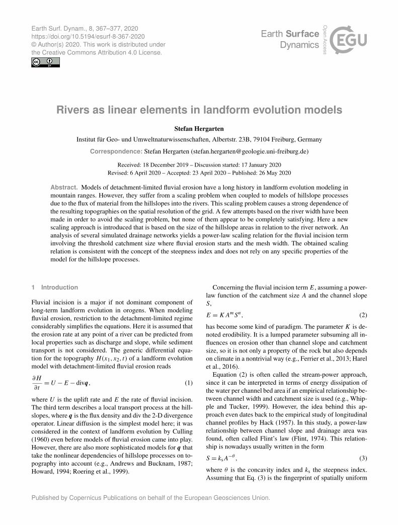
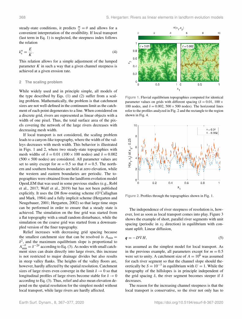
If local transport is not considered, the scaling problemleads to a canyon-like topography, where the width of the val-leys decreases with mesh width. This behavior is illustratedin Figs. 1 and 2, where two steady-state topographies withmesh widths of δ = 0.01 (100× 100 nodes) and δ = 0.002(500× 500 nodes) are considered. All parameter values areset to unity except for m= 0.5 so that θ = 0.5. The north-ern and southern boundaries are held at zero elevation, whilethe western and eastern boundaries are periodic. The to-pographies were obtained from the landform evolution modelOpenLEM that was used in some previous studies (e.g., Roblet al., 2017; Wulf et al., 2019) but has not been publishedexplicitly. It uses the D8 flow-routing scheme (O’Callaghanand Mark, 1984) and a fully implicit scheme (Hergarten andNeugebauer, 2001; Hergarten, 2002) so that large time stepscan be performed in order to ensure that a steady state isachieved. The simulation on the fine grid was started froma flat topography with a small random disturbance, while thesimulation on the coarse grid was started from a downsam-pled version of the finer topography.

Relief increases with decreasing grid spacing becausethe smallest catchment size that can be resolved is Amin =

δ2, and the maximum equilibrium slope is proportional toA−θmin = δ

−2θ according to Eq. (3). As nodes with small catch-ment sizes can drain directly into large rivers, this increaseis not restricted to major drainage divides but also resultsin steep valley flanks. The heights of the valley floors are,however, hardly affected by the spatial resolution. Catchmentsizes of large rivers even converge in the limit δ→ 0 so thatlongitudinal profiles of large rivers become stable for δ→ 0according to Eq. (3). Thus, relief and also mean elevation de-pend on the spatial resolution for the simplest model withoutlocal transport, while large rivers are hardly affected.

Figure 1. Fluvial equilibrium topographies computed for identicalparameter values on grids with different spacing (δ = 0.01, 100×100 nodes, and δ = 0.002, 500× 500 nodes). The horizontal linesrefer to the profiles analyzed in Fig. 2 and the rectangle to the regionshown in Fig. 4.

Figure 2. Profiles through the topographies shown in Fig. 1.

The independence of river steepness of resolution is, how-ever, lost as soon as local transport comes into play. Figure 3shows the example of short, parallel river segments with unitspacing (periodic in x2 direction) in equilibrium with con-stant uplift. Linear diffusion,

q =−D∇H, (5)

was assumed as the simplest model for local transport. Asin the previous example, all parameters except for m= 0.5were set to unity. A catchment size of A= 106 was assumedfor each river segment so that the channel slope should the-oretically be S = 10−3 in equilibrium with U = 1. While thetopography of the hillslopes is in principle independent ofthe grid spacing δ, the river segment becomes steeper if δdecreases.

The reason for the increasing channel steepness is that thelocal transport is conservative, so the river not only has to

Earth Surf. Dynam., 8, 367–377, 2020 https://doi.org/10.5194/esurf-8-367-2020

S. Hergarten: Rivers as linear elements in landform evolution models 369

Figure 3. River segments in equilibrium with uplift for differentmesh widths δ.

incise into the rock at its bed but also has to remove the ma-terial coming from the hillslopes. Regardless of the modelused for local transport, a flux of (d − δ)U per river lengthenters the site that contains the river in equilibrium, where dis the valley spacing. Then the discretized divergence of theflux density is

divq =−(d − δ)U

δ. (6)

Inserting this result into the steady-state version of Eq. (1)yields

E = U − divq =d

δU, (7)

so the fluvial erosion rate required for compensating uplift ishigher than it would be without local transport by a factor d

δ.

This requires an increase in the channel slope by a factor of(dδ

) 1n according to Eq. (2).

This scaling issue has been known for more than 25 years,and two approaches have been suggested to overcome theproblem. Howard (1994) suggested a subpixel representationof the rivers, where a river segment only covers a fraction ofa grid cell. It was assumed that this fraction is w

δ, where w

is the river width, and then the fluvial incision term E wasmultiplied by this factor. Perron et al. (2008) transferred thisconcept to the detachment-limited case. According to Eq. (7),rescaling E by the factor w

δyields

E =d

wU, (8)

so the dependency on δ indeed vanishes.While straightforward at first sight, this scaling approach

is not free of problems. The channel width in general in-creases in the downstream direction so that equilibrium riverprofiles are no longer consistent with Eq. (3). Perron et al.(2008) avoided this problem by assuming a constant channelwidth and postponing it to subsequent studies. As discussed

by Pelletier (2010), taking an increase in channel width in thedownstream direction into account would require a reductionof the exponentm in Eq. (2) in order to keep it consistent withEq. (3). However, the unit and meaning of the erodibility Kwould change then.

In order to overcome this problem, Pelletier (2010) sug-gested leaving the fluvial incision term as is and rescaling thelocal transport term divq by the inverse factor δ

wat sites con-

taining rivers. Practically, this rescaling means that the fluxof material coming from the hillslopes is not distributed overthe entire grid cell but only over the part of the area coveredby the river. Thus it can be seen as the inverse of the subpixelapproach of Howard (1994) and Perron et al. (2008) appliedto the local transport instead of the fluvial erosion. For thesteady-state example considered above, this rescaling leadsto

divq =−(d − δ)U

w, (9)

instead of Eq. (6), so that

E = U − divq =(d +w− δ)

wU. (10)

For w� d and δ� d, however, this relation approachesEq. (8), so this concept suffers from the same problem asthe approach of Howard (1994) and Perron et al. (2008).

Thus there seems to be no completely satisfactory solutionof the scaling problem so far. Several contemporary model-ing studies (e.g., Duvall and Tucker, 2015; Gray et al., 2018;Wulf et al., 2019; Reitman et al., 2019) use neither of the twoapproaches but implement Eq. (1) as is without taking its de-pendence on the grid scale into account. This is not a crucialproblem as long as simulations with different spatial resolu-tions are not compared and as long as we are aware that theerodibilityK has a limited meaning. As soon as the relevanceof fluvial erosion and hillslope processes is assessed quanti-tatively or scaling relations are developed (e.g., Theodoratoset al., 2018), the problem may become crucial. A further dis-cussion is given in Sect. 5.

Other recent approaches navigate around the scaling prob-lem by neglecting the flux of material from the hillslopesinto the rivers. The recently presented landform evolutionmodel TTLEM (Campforts et al., 2017) makes a distinctionby catchment size in such a way that fluvial erosion only actson sites with a catchment size above a given threshold Ac,while hillslope processes only act at smaller catchment sizes.It is assumed that all hillslope material entering the riversis immediately excavated without any further effect so thatfluxes from hillslopes into rivers can be disregarded and thescaling problem does not occur. This approach reduces theinteraction between rivers and hillslopes to a one-way cou-pling, where only the rivers have an influence on the evolu-tion of the hillslopes and can be seen as an implementation ofbedrock incision in the strict sense. While it seems that theterms detachment-limited erosion and bedrock incision are

https://doi.org/10.5194/esurf-8-367-2020 Earth Surf. Dynam., 8, 367–377, 2020

370 S. Hergarten: Rivers as linear elements in landform evolution models

sometimes used synonymously, it should be clarified that theapplicability of the concept of pure bedrock incision is prob-ably much narrower than that of detachment-limited erosion,in particular if highly resistant material is brought into thechannels (Shobe et al., 2016). The same in principle holdsfor the model most widely used in the context of drainagedivide migration (Goren et al., 2014), where analytical solu-tions for hillslope processes are used on the subpixel scale.

3 A new scaling approach

The simple example considered in the previous section in-volves a dependence on grid spacing δ according to the fac-tor d

δwithout rescaling (Eq. 7). Both approaches for rescaling

replace the dependence on δ by a dependence on the channelwidth w so that a factor d

wremains (Eq. 8). This is, how-

ever, still a problem if w is not constant. The occurrence ofthe factor d

wsuggests that the valley spacing d would be a

more suitable characteristic length scale for rescaling than wif we want to preserve the form of the erosion law (Eq. 2)without changing the exponents m and n. In the following, aconcept that generalizes the simple example of parallel riversto dendritic networks is developed.

Let us start from the simplest approach to distinguishchannel sites from hillslopes by defining a threshold catch-ment size Ac in such a way that all sites with A≥ Ac areriver segments, while all sites with A<Ac belong to hill-slopes. As local transport is conservative, all material erodedanywhere has to be removed by the river sites so that wehave to determine how much material each river site receivesfrom the hillslopes. The area of the respective hillslopes canbe determined for a given topography without any specificassumptions on the transport process except for the directionof transport. The simplest model is to assume that local trans-port follows the hypothetic channel network at the hillslopes,i.e., the direction of steepest descent on a purely fluvial to-pography. Figure 4 illustrates this concept. Each colored areaconsists of one channel site and the hillslope area that deliv-ers its eroded material to this site, i.e, of those sites that draininto the considered site without passing any other upstreamchannel site.

If the size of this area was the same for each river site,rescaling the fluvial erosion rate (Eq. 2) according to

E = AeKAmSn, (11)

where Ae is the size of this area measured in DEM (digitalelevation model) pixels (i.e., the number of sites), would al-ready solve the scaling problem. However, it is immediatelyrecognized in Fig. 4 that the sizes of these areas are highlyvariable. A random variation in these sizes is not a problem.If Ae in Eq. (11) is the mean size, channel steepness will justvary randomly, which is also found in nature. A systematicdependence of Ae on catchment size would, however, be aproblem. In this case, equilibrium river profiles would be no

Figure 4. Flow pattern of the central region of Fig. 1. Black linesshow rivers with A≥ Ac for Ac = 100 pixels. Gray lines are chan-nels withA<Ac, considered to be hillslope sites. Each colored areaconsists of one channel site plus the hillslope area that drains intothis site without passing another upstream channel site.

longer consistent with Eq. (3), so the problem would be basi-cally the same as in the previous approach for a non-constantchannel width.

In the following, numerically obtained equilibriumdrainage networks are analyzed in order to find out how Aedepends on A and on Ac. More precisely, Ae is the meansize of all hillslope areas draining into channel sites with agiven catchment size A at a given fluvial threshold Ac (plusthe respective channel site). For simplicity, all areas are mea-sured in DEM pixels in the following considerations, i.e.,as a number of sites. The starting point of the analysis isthe drainage network of a fluvial equilibrium topography ona square L×L grid with L= 10000. Boundary conditionsand parameter values except for the grid size are the same asthose in the smaller examples shown in Fig. 1.

Figure 5 reveals that the eroded area Ae increases withthe fluvial threshold Ac but becomes independent of A ifthe catchment size A is sufficiently large. This means thatthe hillslopes draining into large rivers are not systematicallylarger than those draining into small rivers. It is the reasonwhy we will arrive at a scaling relation that preserves theform of Eq. (2) and avoids the problem occurring if the riverwidth is used for scaling.

The increase in Ae if A approaches Ac can be explainedby distinguishing between river segments and channel heads.Let us define channel heads as those sites without any tribu-tary with A≥ Ac, i.e., as those sites that are only supplied byhillslopes. All other sites with A≥ Ac are considered to beriver segments. All sites with A= Ac are channel heads andthus follow the relation Ae = A so that all curves start at thedotted line in Fig. 5. The resulting values Ae of the river seg-ments (without the channel heads) are shown by the dashed

Earth Surf. Dynam., 8, 367–377, 2020 https://doi.org/10.5194/esurf-8-367-2020

S. Hergarten: Rivers as linear elements in landform evolution models 371

Figure 5. Eroded area Ae as a function of the catchment size A fordifferent fluvial thresholds Ac. Raw data were used for the catch-ment sizes that occurred at least 1000 times on the grid. Otherwise,data were binned dynamically so that there are at least 1000 pointsin each bin.

lines in Fig. 5. The increase in Ae if A approaches Ac eventurns into a decrease then. This decrease, which arises fromthe limitation Ae ≤ A−Ac, holds for all river segments thathave at least one tributary cell contributing at least Ac. Thusthe contribution of the hillslopes must be small if A is onlyslightly larger than Ac. However, the decrease is exaggeratedby the logarithmic scale and concerns only a small numberof sites, so it makes sense to assume that Ae is independentof A for river segments.

Both the number of river segment sites and the numberof channel head sites decrease with an increasing thresholdAc. The decrease in the latter is faster so that the ratio ofthe numbers of head sites to river sites converges to zero forlargeAc values. This is, however, not true for the total contri-butions. Figure 6 shows the ratio of the sum of the Ae valuesof all river segments to the sum of the Ae values of the chan-nel heads. It can also be interpreted as the ratio of the totalarea that must be eroded by the river segments to the totalarea that must be eroded by the channel heads. The resultsshown for different grid sizes shown in Fig. 6 suggest thatthis ratio becomes constant in the limit of large grid sizes. Itapparently approaches a value of about 2 here, which meansthat the river segments contribute about two-thirds, and thechannel heads one-third, to total fluvial erosion.

This result suggests that the dependency of Ae on thethreshold Ac is determined by the cumulative distributionP (A) of the catchment sizes in the drainage network. Thisdistribution describes the probability that a randomly se-lected site has a catchment size ≥ A. The probability P (Ac)evaluated at the fluvial threshold is the ratio of the area cov-ered by all channel pixels to the total area. It can be inter-preted as a drainage density (river length per total area) ona discrete grid. Then a fraction P (Ac) of the considered do-main must erode a given fraction (here about two-thirds) of

Figure 6. Ratio of total area eroded by all river segments to totalarea eroded by all channel head sites as a function of the fluvialthreshold Ac.

the domain, leading to the relation

Ae =γ

P (Ac), (12)

with γ ≈ 23 for this network. While Ae can be measured

directly for the considered drainage network, its relationto P (A) (Eq. 12) is useful, as this distribution has alreadybeen investigated in several studies on natural and modeleddrainage networks (Rodriguez-Iturbe et al., 1992a; Maritanet al., 1996b; Rodriguez-Iturbe and Rinaldo, 1997; Rinaldoet al., 1998; Hergarten and Neugebauer, 2001; Hergarten,2002; Hergarten et al., 2014, 2016). It was found that P (A)follows a power-law distribution,

P (A)∼ A−β , (13)

over a reasonable range, where a range β ∈ [0.41,0.46] wasfound except for the two latest studies. In these studies, largernetworks were considered to be making use of increasingdata availability and computing capacities. An exponent veryclose to 0.5 was found for both optimal channel networks(OCNs; see below) (Hergarten et al., 2014) and a real riverpattern at the continental scale (Hergarten et al., 2016).

Equations (12) and (13) suggest a power-law relation,

Ae = αAβc , (14)

between the eroded area and the fluvial threshold. The va-lidity of Eqs. (12), (13), and (14) is investigated in Fig. 7.Comparing the two solid curves reveals that Eq. (12) doesnot hold exactly, since the curves come closer to each otherfor decreasing catchment sizes. The reason for this is that Aeonly refers to the river segments without the channel headsso that P (Ac) in Eq. (12) should also exclude the channelhead sites. The dashed colored line in Fig. 7 showing the ac-cordingly reduced distribution P (A) illustrates that Eq. (12)indeed holds then and that the effect vanishes for large Acvalues.

https://doi.org/10.5194/esurf-8-367-2020 Earth Surf. Dynam., 8, 367–377, 2020

372 S. Hergarten: Rivers as linear elements in landform evolution models

Figure 7. Black axes: eroded area as a function of the fluvial thresh-old. Colored axes: cumulative distribution of the catchment sizes.

The black dashed line in Fig. 7 refers to the best-fit power-law relation according to Eq. (14). It is based on all inte-ger values of Ac from 1 to 10 000, assuming equal errors, sothat the large values of Ac practically have a high weight inthe fit. The power law with the obtained values α = 1.360and β = 0.465 fits the data well, with a relative error ofless than 5 % for Ac ∈ [15,10000] and less than 1 % forAc ∈ [400,10000]. The deviations are larger for smaller flu-vial thresholds due to the fact that dendritic networks cannotbe represented well on a regular lattice at small scales.

The relation to the catchment-size distribution (Eqs. 12and 13) suggests that the power-law dependency of Ae on Ac(Eq. 14) should be universal. For testing this hypothesis, a setof equilibrium topographies with θ ∈ {0.25,0.45,0.5,0.75}was analyzed. These values cover the range that has beenfound so far under relatively homogeneous conditions (e.g.,Robl et al., 2017). The value θ = 0.45 was added, as it is of-ten used as a reference value instead of θ = 0.5 (e.g., Whip-ple et al., 2013; Lague, 2014). Parameter values and bound-ary conditions are the same as in the previous example. Sincethe exponent n has no immediate effect on equilibrium to-pographies, values n 6= 1 were not considered.

The power-law parameters α and β obtained from equi-librium topographies on different lattice sizes L are given inTable 1. In addition, the original data for the largest grids areshown in Fig. 8. The results are overall similar, with a ten-dency to lower exponents β for increasing θ . A notable devia-tion is only found for the very high concavity index θ = 0.75.Here the slopes become very steep at small catchment sizes,resulting in a slower migration of drainage divides during thesimulation (Robl et al., 2017). As a result, the topographyreaches a steady state quite soon so that there is finally lessreorganization in the drainage network with regard to the ini-tial random pattern. In this sense, the lower exponents foundfor θ = 0.75 can be seen as a fingerprint of poorly organizedriver patterns but are probably not relevant for the rivers that

Table 1. Parameter values of the power-law relation between erodedarea and fluvial threshold (Eq. 14) obtained from different simulateddrainage networks on regular lattices with L×L nodes.

θ L α β

Stea

dy-s

tate

topo

grap

hies

0.255000 1.264 0.4922000 1.072 0.5111000 1.587 0.470

0.455000 1.273 0.4782000 1.586 0.4511000 1.047 0.499

0.50

10 000 1.360 0.4655000 1.434 0.4592000 1.807 0.4231000 1.579 0.440

0.75

10 000 1.653 0.3935000 1.715 0.3882000 1.433 0.4121000 2.179 0.359

OC

Ns 0.14

4096

1.487 0.4800.33 1.626 0.4730.50 1.508 0.4780.60 1.521 0.475

Figure 8. Eroded area Ae as a function of the fluvial threshold Acfor the considered drainage networks. For clarity, only the resultsobtained from the largest domains are plotted.

were the empirical basis of the stream-power law. These find-ings confirm that the concavity index θ has a minor effect onthe topology of the drainage networks, although it stronglyaffects the shape of longitudinal river profiles and thus thetopography.

In addition, Table 1 and Fig. 8 also contain results ob-tained from optimal channel networks (OCNs) on a gridwith L= 4096. Optimal channel networks are derived fromthe principle of minimum energy dissipation and have beenwidely used in the context of river networks (e.g., Howard,

Earth Surf. Dynam., 8, 367–377, 2020 https://doi.org/10.5194/esurf-8-367-2020

S. Hergarten: Rivers as linear elements in landform evolution models 373

Table 2. Parameter values of the power-law relation between erodedarea and fluvial threshold (Eq. 14) obtained from different simulateddrainage networks on triangular lattices with N nodes for θ = 0.5.

N α β

2× 107 1.630 0.4331× 107 1.611 0.4355× 106 1.264 0.4662× 106 1.332 0.4541× 106 1.400 0.4455× 105 1.432 0.450

1990; Rodriguez-Iturbe et al., 1992c, b; Rinaldo et al., 1992,1998; Maritan et al., 1996a, b). The networks considered hereare those shown in Fig. 1 of Hergarten et al. (2014), whereθ is related to the parameter n used there by θ = n−1

n+1 . Thevalues of Ae of OCNs are overall slightly higher than thoseof the equilibrium topographies, and the variation with θ islower. As OCNs are organized more strongly than drainagenetworks of arbitrary equilibrium topographies, the lowervariability among OCNs is not surprising.

Table 2 provides additional results obtained from steady-state topographies on triangulated irregular networks (TINs).Numbers of neighbors, distances to neighbors, and areas ofpixels are variable here. Areas of pixels are defined by theVoronoi diagram. Nondimensional areas (in DEM pixels) arenormalized to the mean pixel size given by δ2

=AtotN

, whereAtot is total area and N the number of nodes. The valueslisted in Table 2 and the respective curve in Fig. 8 show thatthe results obtained from TINs are close to those obtainedfrom regular meshes.

These results suggest defining the values α = 1.508 andβ = 0.478 obtained from the OCN with θ = 0.5 as referencevalues. The question is, however, whether such precision isuseful for applications. In particular, β = 0.5 would be moreconvenient than lower values. In the considerations madeabove, all areas are measured in DEM pixels and are thusnondimensional properties. Considering Ac to be a physical(dimensional) area, Ac has to be replaced by Ac

δ2 in Eq. (14).Then the fluvial erosion rate (Eq. 11) turns into

E = α

(Ac

δ2

)βKAmSn, (15)

so that the fluvial incision term scales like δ−2β . For β = 0.5,the fluvial term scales like 1

δ. This is not only convenient

but also leads to basically the same scaling relation assumedby Perron et al. (2008). The only difference is that the termα√Ac occurring here was interpreted as a channel width w

and then assumed to be constant for all rivers so that it lostits physical meaning. Thus the new formulation of the fluvialincision term also fixes the concern raised by Pelletier (2010)that led to the alternative formulation where the hillslopetransport term was rescaled.

In order to estimate α for β = 0.5, it is helpful to knowwhich region of Fig. 8 is occupied by typical model appli-cations. A breakdown of Flint’s law (Eq. 3) was reportedat catchment sizes between between about 0.1 and 5 km2

(Montgomery and Foufoula-Georgiou, 1993; Stock and Di-etrich, 2003; Wobus et al., 2006). However, channel steep-ness declines at small catchment sizes, so this breakdown im-plies that other erosion processes come into play rather thanthat fluvial erosion is no longer active. In turn, many smallsprings in mountain regions have discharges on the order ofmagnitude of 0.1 L s−1 (e.g., Hergarten et al., 2016), corre-sponding to catchment sizes A< 0.01 km2, but it is not clearwhether the erosive action of the resulting small streams fol-lows Flint’s law. Reasonable estimates of Ac are probablybetween these two ranges. Assuming a spatial resolution ofabout 100 m or a bit less, Ac will be on the order of magni-tude of a few to 100 DEM pixels. As illustrated by the blackline in Fig. 8, α =

√2 provides a reasonable estimate for this

range with simple numbers as αAβc =√

2Ac. With this esti-mate, the scaling factor for the fluvial erosion rate is

√2Acδ

,and the modified stream-power law for fluvial erosion turnsinto

E =

√2Ac

δKAmSn. (16)

4 Numerical examples

Let us first return to the example of parallel rivers consid-ered in Fig. 3. It was found in Sect. 2 that the topography ofthe hillslopes was robust against the spatial resolution, whilethe channel slope increases with decreasing grid spacing δ.Both approaches previously published fix this problem, butthe channel slopes are too steep by a factor of d

wcompared

to what is expected from the erodibility.It should be noted that this example is not related to the

approach to estimate Ae from Ac for dendritic networks(Eqs. 15 and 16) but can only test the validity of the prin-cipal scaling approach (Eq. 11). The size of the area Ae doesnot follow Eq. (14) but is defined by the geometry as Ae =

dδ

(measured in DEM pixels). Figure 9 shows the numerical re-sults for the parameter values used in Fig. 3 for different val-ues of δ. The simulation was started from a flat topographywhere the flow paths of the parallel rivers are predefined. Asthe problem is linear for n= 1, this example can also be seenas the change in the river profile over time if uplift suddenlyincreases at t = 0, while the base level remains constant. Theresults show that the equilibrium profile achieved for longtimes is reproduced correctly and that the time-dependent be-havior is also robust against the resolution. This means thatthe scaling approach itself (Eq. 11) yields both the correctequilibrium behavior and the correct timescale.

https://doi.org/10.5194/esurf-8-367-2020 Earth Surf. Dynam., 8, 367–377, 2020

374 S. Hergarten: Rivers as linear elements in landform evolution models

Figure 9. Numerical results for the scenario considered in Fig. 3.The river profiles obtained for δ = 0.025 and δ = 0.01 cannot bedistinguished visually.

The second example refers to the scenario considered inFig. 1 but extended by a fluvial threshold Ac = 10−5 andby linear diffusion with a diffusivity D = 10−5. The thresh-old Ac is a property of the fluvial erosion process, while thediffusive hillslope process is not related to it. It is thus as-sumed that fluvial erosion acts only at sites where A≥ Ac,while diffusion is active everywhere. A TIN representation isused in order to avoid artifacts from the combination of theeight-neighbor (D8) flow-routing scheme with the standardfour-neighbor diffusion scheme on a regular mesh. The sim-ulations are started from an almost flat topography with unituplift. Uplift is switched off at t = 50 in order to observe thedecay of the topography.

The mean steepness index ks of the large rivers is plot-ted as a function of time in Fig. 10. Large rivers are de-fined by A≥ 10−3 here, which is considerably larger thanAc but much smaller than the domain. As expected, the sim-ulations performed without any rescaling of the erodibility(dashed lines) are strongly affected by the spatial resolution.The steepness index increases with an increasing number ofnodes N , i.e., with decreasing pixel size. In turn, the re-sults obtained using the simple scaling relation (Eq. 16; solidlines) have a much weaker dependence on resolution. Thereis, however, a residual variation in channel steepness. Themean value of ks varies between about 1.6 and 2.0 over theconsidered range from N = 105 to N = 107. This result doesnot change fundamentally if a higher or lower threshold thanA≥ 10−3 is used for defining large rivers.

5 Discussion

It may be surprising that the example of fluvial incision andhillslope diffusion considered in the previous section yieldsa mean steepness index greater than 1, although the scalingconcept was developed in order to preserve channel steep-ness. The concept is, however, based on a generic hillslope

Figure 10. Mean steepness index ks of the large rivers obtainedfrom simulations on TINs with different resolutions, defined by thetotal number of nodes N . Solid lines refer to the simplified scalingapproach suggested in this paper (Eq. 16), while dashed lines re-fer to simulations performed without any rescaling. The latter areplotted only for N ≤ 106.

process where the direction of transport follows a hypotheticfluvial equilibrium pattern and turns into fluvial erosion at agiven threshold catchment sizeAc. It is questionable whetherany hillslope process occurring in nature comes close to thissimple model. In the example considered here, the diffusionprocess is characterized by a diffusivity D and is not relatedto Ac. The fluvial domain is affected by diffusion more andmore with increasing diffusivity. As a consequence, slopesof small channels decrease so that they erode less efficiently.This has to be compensated by the larger rivers so that theybecome steeper.

This is, however, a real property of the hillslope processhere, and it is not the goal of the scaling approach to removeit. The concept presented here aims at removing the depen-dence on the resolution and providing the way in which val-ues of the erodibility should be interpreted. Here it is sug-gested that they should be considered in combination witha fluvial threshold Ac in such a way that they would yieldthe expected channel steepness if the generic hillslope modelwere valid.

In turn, the residual dependence of channel steepness onresolution is a problem, in particular because it is not clearwhether it converges in the limit δ→ 0 (N→∞). The prob-lem arises from network reorganization, which also affectsthe fluvial region. Diffusion disturbs the dendritic topologytowards parallel flow where the model based on Hack’s find-ings (Eq. 2) is not valid. Using an improved flow-routingscheme that is able to distinguish channelized flow from par-allel flow as suggested by Pelletier (2010) and letting Acself-adjust might reduce the problem. However, the aim ofthis study is to develop a simple, quite universal rescalingapproach that avoids or at least reduces the dependence on

Earth Surf. Dynam., 8, 367–377, 2020 https://doi.org/10.5194/esurf-8-367-2020

S. Hergarten: Rivers as linear elements in landform evolution models 375

resolution without modifying the applied model seriously. Inthis sense, Eq. (16) should be a good trade-off.

Nevertheless it is important to keep the difference be-tween detachment-limited erosion and pure bedrock incisionin mind. Here it is assumed that the ability of the river to takeup particles and carry them away concerns both the riverbedand material coming from adjacent hillslopes. If we, con-versely, assume that all material coming from the hillslopesis instantaneously removed by the river without any conse-quences, there is no feedback of the hillslopes to the rivers,and Eq. (1) does not require any rescaling.

The results of this study have consequences for scaling re-lations in coupled models of rivers and hillslopes. Theodor-atos et al. (2018) conducted a comprehensive analysis of theproblem with linear diffusion without rescaling. The param-eters they used were the same as in the previous example(Fig. 10), so it is immediately clear that their numerical re-sults strongly depend on resolution. The authors argued that,following the approach of Pelletier (2010), both grid spac-ing and channel width are rescaled so that the ratio δ

wre-

mains constant, and the scaling issue is consistent through-out all scales. However, the results presented here show thatthe property relevant for compensating δ is not channel widthbut Ae and thus Ac. These parameters are, however, physicalproperties of the erosion process, so they do not scale withthe size of the domain. As a consequence, the characteristichorizontal length scale of the coupled system should ratherbe

lc =D√AcK

, (17)

for m= 0.5 and n= 1 instead of lc =√DK

used by Theodor-atos et al. (2018). This problem also affects the recent ex-tension by an erosion threshold (Theodoratos and Kirchner,2020).

6 Conclusions

This study presents a simple scaling relation for the flu-vial incision term in landform evolution models involvingdetachment-limited fluvial erosion and hillslope processes.In order to avoid a dependence of the simulated topographieson the spatial resolution of the grid, the fluvial incision termmust be multiplied by a scaling factor depending on the ra-tio of the threshold catchment size Ac where fluvial erosionstarts and the pixel size δ2 of the grid. The analysis of severalsimulated drainage networks yields a power-law dependenceof the scaling factor in Eq. (15) with an exponent slightlylower than 0.5. However, for application in numerical mod-els, a simpler approximation where the fluvial erosion rate isrescaled by a factor

√2Acδ

is suggested. As this relation as-sumes a simple, generic hillslope process, it cannot providean exact solution for all types of hillslope processes. In com-bination with such processes, e.g., diffusion, the dependence

on the spatial resolution is not completely removed. Never-theless, the simple scaling relation appears to be a reasonabletrade-off between accuracy and simplicity.

Code and data availability. All codes and computed data can bedownloaded from the FreiDok data repository 155182 (Hergarten,2020). The author is happy to support interested readers in repro-ducing the results and performing subsequent research.

Competing interests. The author declares that there is no con-flict of interest.

Acknowledgements. The author would like to thank the twoanonymous reviewers for their thorough consideration and for theirvery constructive suggestions to improve the readability of the pa-per. The author would also like to thank Wolfgang Schwanghart forthe editorial handling.

Review statement. This paper was edited by Wolfgang Schwang-hart and reviewed by Taylor Perron and two anonymous referees.

References

Andrews, D. J. and Bucknam, R. C.: Fitting degradation of shore-line scarps by a nonlinear diffusion model, J. Geophys. Res., 92,12857–12867, https://doi.org/10.1029/JB092iB12p12857, 1987.

Campforts, B., Schwanghart, W., and Govers, G.: Accurate simu-lation of transient landscape evolution by eliminating numericaldiffusion: the TTLEM 1.0 model, Earth Surf. Dynam., 5, 47–66,https://doi.org/10.5194/esurf-5-47-2017, 2017.

Culling, W.: Analytical theory of erosion, J. Geol., 68, 336–344,https://doi.org/10.1086/626663, 1960.

Duvall, A. R. and Tucker, G. E.: Dynamic ridges and valleys ina strike-slip environment, J. Geophys. Res.-Earth, 120, 2016–2026, https://doi.org/10.1002/2015JF003618, 2015.

Ferrier, K. L., Perron, J. T., Mukhopadhyay, S., Rosener, M., Stock,J. D., Huppert, K. L., and Slosberg, M.: Covariation of climateand long-term erosion rates across a steep rainfall gradient onthe Hawaiian island of Kaua´i, GSA Bull., 125, 1146–1163,https://doi.org/10.1130/B30726.1, 2013.

Flint, J. J.: Stream gradient as a function of order, mag-nitude, and discharge, Water Resour. Res., 10, 969–973,https://doi.org/10.1029/WR010i005p00969, 1974.

Goren, L., Willett, S. D., Herman, F., and Braun, J.: Cou-pled numerical–analytical approach to landscape evo-lution modeling, Earth Surf. Proc. Land., 39, 522–545,https://doi.org/10.1002/esp.3514, 2014.

Gray, H. J., Shobe, C. M., Hobley, D. E. J., Tucker, G. E.,Duvall, A. R., Harbert, S. A., and Owen, L. A.: Off-fault deformation rate along the southern San Andreas faultat Mecca Hills, southern California, inferred from land-scape modeling of curved drainages, Geology, 46, 59–62,https://doi.org/10.1130/G39820.1, 2018.

https://doi.org/10.5194/esurf-8-367-2020 Earth Surf. Dynam., 8, 367–377, 2020

376 S. Hergarten: Rivers as linear elements in landform evolution models

Hack, J. T.: Studies of longitudinal profiles in Virginiaand Maryland, no. 294-B in US Geol. Survey Prof. Pa-pers, US Government Printing Office, Washington D.C.,https://doi.org/10.3133/pp294B, 1957.

Harel, M.-A., Mudd, S. M., and Attal, M.: Global analy-sis of the stream power law parameters based on world-wide 10Be denudation rates, Geomorphology, 268, 184–196,https://doi.org/10.1016/j.geomorph.2016.05.035, 2016.

Hergarten, S.: Self-Organized Criticality in Earth Sys-tems, Springer, Berlin, Heidelberg, New York,https://doi.org/10.1007/978-3-662-04390-5, 2002.

Hergarten, S.: Rivers as linear elements in landform evolutionmodels: codes and data, FreiDok plus, UniversitätsbibliothekFreiburg, https://doi.org/10.6094/UNIFR/155182, 2020.

Hergarten, S. and Neugebauer, H. J.: Self-organized criti-cal drainage networks, Phys. Rev. Lett., 86, 2689–2692,https://doi.org/10.1103/PhysRevLett.86.2689, 2001.

Hergarten, S., Winkler, G., and Birk, S.: Transferring the conceptof minimum energy dissipation from river networks to subsur-face flow patterns, Hydrol. Earth Syst. Sci., 18, 4277–4288,https://doi.org/10.5194/hess-18-4277-2014, 2014.

Hergarten, S., Winkler, G., and Birk, S.: Scale invariance of sub-surface flow patterns and its limitation, Water Resour. Res., 52,3881–3887, https://doi.org/10.1002/2015WR017530, 2016.

Howard, A. D.: Theoretical model of optimal drainagenetworks, Water Resour. Res., 26, 2107–2117,https://doi.org/10.1029/WR026i009p02107, 1990.

Howard, A. D.: A detachment-limited model for drainagebasin evolution, Water Resour. Res., 30, 2261–2285,https://doi.org/10.1029/94WR00757, 1994.

Lague, D.: The stream power river incision model: evidence,theory and beyond, Earth Surf. Proc. Land., 39, 38–61,https://doi.org/10.1002/esp.3462, 2014.

Maritan, A., Colaiori, F., Flammini, A., Cieplak, M., and Banavar,J. R.: Universality classes of optimal channel networks, Science,272, 984–986, https://doi.org/10.1126/science.272.5264.984,1996a.

Maritan, A., Rinaldo, A., Rigon, R., Giacometti, A., and Rodriguez-Iturbe, I.: Scaling laws for river networks, Phys. Rev. E, 53,1510–1515, https://doi.org/10.1103/PhysRevE.53.1510, 1996b.

Montgomery, D. R. and Foufoula-Georgiou, E.: Channel networksource representation using digital elevation models, Water Re-sour. Res., 29, 3925–3934, https://doi.org/10.1029/93WR02463,1993.

O’Callaghan, J. F. and Mark, D. M.: The extraction of drainagenetworks from digital elevation data, Comput. Vision Graph.,28, 323–344, https://doi.org/10.1016/S0734-189X(84)80011-0,1984.

Pelletier, J. D.: Minimizing the grid-resolution de-pendence of flow-routing algorithms for geomor-phic applications, Geomorphology, 122, 91–98,https://doi.org/10.1016/j.geomorph.2010.06.001, 2010.

Perron, J. T., Dietrich, W. E., and Kirchner, J. W.: Controls onthe spacing of first-order valleys, J. Geophys. Res.-Earth, 113,F04016, https://doi.org/10.1029/2007JF000977, 2008.

Reitman, N. G., Mueller, K. J., Tucker, G. E., Gold, R. D., Briggs,R. W., and Barnhart, K. R.: Offset channels may not accuratelyrecord strike-slip fault displacement: Evidence from landscape

evolution models, J. Geophys. Res.-Sol. Ea., 124, 13427–13451,https://doi.org/10.1029/2019JB018596, 2019.

Rinaldo, A., Rodriguez-Iturbe, I., Bras, R. L., Ijjasz-Vasquez,E., and Marani, A.: Minimum energy and fractal structuresof drainage networks, Water Resour. Res., 28, 2181–2195,https://doi.org/10.1029/92WR00801, 1992.

Rinaldo, A., Rodriguez-Iturbe, I., and Rigon, R.: Chan-nel networks, Annu. Rev. Earth Pl. Sc., 26, 289–327,https://doi.org/10.1146/annurev.earth.26.1.289, 1998.

Robl, J., Hergarten, S., and Prasicek, G.: The topographic state offluvially conditioned mountain ranges, Earth Sci. Rev., 168, 290–317, https://doi.org/10.1016/j.earscirev.2017.03.007, 2017.

Rodriguez-Iturbe, I. and Rinaldo, A.: Fractal River Basins. Chanceand Self-Organization, Cambridge University Press, Cambridge,UK, New York, USA, Melbourne, Australia, 1997.

Rodriguez-Iturbe, I., Ijjasz-Vasquez, E., Bras, R. L., and Tar-boton, D. G.: Power law distribution of mass and en-ergy in river basins, Water Resour. Res., 28, 1089–1093,https://doi.org/10.1029/91WR03033, 1992a.

Rodriguez-Iturbe, I., Rinaldo, A., Rigon, R., Bras, R. L., Ijjasz-Vasquez, E., and Marani, A.: Fractal structures as least energypatterns: The case of river networks, Geophys. Res. Lett., 19,889–892, https://doi.org/10.1029/92GL00938, 1992b.

Rodriguez-Iturbe, I., Rinaldo, A., Rigon, R., Bras, R. L., Marani,A., and Ijjasz-Vasquez, E.: Energy dissipation, runoff production,and the three-dimensional structure of river basins, Water Re-sour. Res., 28, 1095–1103, https://doi.org/10.1029/91WR03034,1992c.

Roering, J. J., Kirchner, J. W., and Dietrich, W. E.: Evidence fornonlinear, diffusive sediment transport on hillslopes and impli-cations for landscape morphology, Water Resour. Res., 35, 853–870, https://doi.org/10.1029/1998WR900090, 1999.

Shobe, C. M., Tucker, G. E., and Anderson, R. S.: Hillslope-derivedblocks retard river incision, Geophys. Res. Lett., 43, 5070–5078,https://doi.org/10.1002/2016GL069262, 2016.

Stock, J. and Dietrich, W. E.: Valley incision by debris flows: Evi-dence of a topographic signature, Water Resour. Res., 39, 1089,https://doi.org/10.1029/2001WR001057, 2003.

Theodoratos, N. and Kirchner, J. W.: Dimensional analysis of alandscape evolution model with incision threshold, Earth Surf.Dynam. Discuss., https://doi.org/10.5194/esurf-2019-80, in re-view, 2020.

Theodoratos, N., Seybold, H., and Kirchner, J. W.: Scaling andsimilarity of a stream-power incision and linear diffusionlandscape evolution model, Earth Surf. Dynam., 6, 779–808,https://doi.org/10.5194/esurf-6-779-2018, 2018.

Whipple, K. X. and Tucker, G. E.: Dynamics of the streampower river incision model: Implications for height lim-its of mountain ranges, landscape response time scalesand research needs, J. Geophys. Res., 104, 17661–17674,https://doi.org/10.1029/1999JB900120, 1999.

Whipple, K. X., DiBiase, R. A., and Crosby, B. T.: Bedrock rivers,in: Fluvial Geomorphology, edited by: Shroder, J. and Wohl, E.,vol. 9 Treatise on Geomorphology, Academic Press, San Diego,CA, USA, 550–573, https://doi.org/10.1016/B978-0-12-374739-6.00226-8, 2013.

Wobus, C., Whipple, K. X., Kirby, E., Snyder, N., Johnson, J., Spy-ropolou, K., Crosby, B., and Sheehan, D.: Tectonics from topog-raphy: Procedures, promise, and pitfalls, in: Tectonics, Climate,

Earth Surf. Dynam., 8, 367–377, 2020 https://doi.org/10.5194/esurf-8-367-2020

S. Hergarten: Rivers as linear elements in landform evolution models 377

and Landscape Evolution, edited by: Willett, S. D., Hovius, N.,Brandon, M. T., and Fisher, D. M., vol. 398 of GSA Special Pa-pers, Geological Society of America, Boulder, Washington, D.C.,USA, 55–74, https://doi.org/10.1130/2006.2398(04), 2006.

Wulf, G., Hergarten, S., and Kenkmann, T.: Combined re-mote sensing analyses and landform evolution modeling re-veal the terrestrial Bosumtwi impact structure as a Mars-like rampart crater, Earth Planet. Sc. Lett., 506, 209–220,https://doi.org/10.1016/j.epsl.2018.11.009, 2019.

https://doi.org/10.5194/esurf-8-367-2020 Earth Surf. Dynam., 8, 367–377, 2020