Risk versus Return: Betting optimally on the Soccer World Cup

using Robust Optimization

Virgile Galle and Ludovica Rizzo

Abstract

The sports betting industry is estimated to be worth between $700 billion and $1 trilliona year internationally. Approximately 70% of this business comes from soccer betting. It isimportant to note that the Soccer World Cup is one of the most lucrative events of the sportsbetting industry. For every single game, it is possible to bet on a multitude of events: the finalscore (as one would expect) as well as the time of the first goal, the number of yellow cards,whether a certain player scores, etc. Current state-of-the art betting approaches, currently relyon stochastic optimization techniques. These approaches are criticized for unnecessary volatilityand inability to handle a large number of simultaneous events that currently take place duringthe World Cup. In this work, we propose a novel risk management approach to sports bettingthat handles risk based on Robust Optimization. A key advantage is that this approach can bescaled to the large number of events that are present in the World Cup while reducing the riskexposure.

Our effective betting uses three components:1. A machine learning model that predicts the probability of an outcome2. The bookmaker’s odds for that outcome3. An optimization algorithm that compares the two numbers above and decides how much tobet

We first create a data-driven predictive model for the outcome of World Cup games. Ourmodel is built based on logistic regression and data from the last 5 World Cups such as thenumber of consecutive participations to the tournament, the qualifying zone and whether ateam is playing in its home continent. On the 2014 World Cup, the model has a notableaccuracy of 68% in predicting the group winners and 50% on the outcome of group stage games.These numbers clearly outperform the corresponding accuracies of 62% and 33% of GoldmanSachs’ prediction team.

Subsequently, we develop a Robust Optimization model for the betting problem. RobustOptimization is a modern decision-making framework that has been widely used in a varietyof settings including portfolio allocations. With a large number of simultaneous bets, we usethe overall accuracy of the predictive model to optimize the worst case gain. This providesa conservative approach that guarantees a minimum gain with high probability. Applied tothe 2014 World Cup, our betting strategy generated a return of 51%. Simulation experimentsdemonstrate that this strategy reduces risk exposure by a factor of 7 compared to a widely usedstochastic optimization approach. Our analysis leads us to believe that Robust Optimization isa novel and valuable approach to modeling betting problems on a large number of simultaneousevents. Combined with a good prediction model, this betting strategy can guarantee significantgains while reducing the risk.

1

1 Introduction and Literature Review

This paper considers the problem of betting on a large number of events with fixed odds, as duringthe Soccer World Cup. A typical setting is the following : a player identifies a set of N events(soccer games here) on which he wants to bet. He has a fixed budget B, and knows the bookmakers’odds for every event (represented as the return on a unit stake and denoted ci). Let us also assumethat the player has a statistical model that gives good estimates on the probability of each event(pi). Comparing these probabilities pi with the odds ci, the player needs to decide his ”bettingstrategy”, ie how to allocate his budget among the different games.

Betting has been widely studied in the Stochastic Optimization literature ( [1], [2], [3] and [4]).It has widespread applications such as portfolio optimization, gambling games or investment strate-gies. However most of the classical approaches do not apply to the problem of betting on a largenumber of simultaneous events. A very common assertion in the literature is that the customershould bet only on events where his expected gain is positive meaning when he has an edge overthe bookmakers (denoted later pici > 1). Efficient predictive models should be able to create thisedge. However, this is not always possible depending on the event that the player bets on. Weshow that theoretically, this condition might not be necessary.

Betting on multiple simultaneous events has only been studied recently. The first step (asexplained in [1]) is to observe that maximizing the expected revenue is an extremely risky approach.In fact, in this case, the optimal strategy is to allocate the entire budget to the event with the highestexpected gain. Using this approach the player doesn’t diversify his risk and, if a repeated bettinggame is considered, will be ruined almost surely. After this step, it is common (see [1], [2], [3])to consider a risk-averse utility function and to look for a strategy that maximizes this expectedutility. The most common utility function is the logarithm leading to the Kelly criterion ( [3], [4])that is broadly used in blackjack for example. However, the Kelly criterion can only be used in thecase of sequential events. In the case of simultaneous events, [1] maximizes the expected gain usinga stochastic gradient-descent approach. This approach is computationally expensive and cannotbe applied to a large number of events. Furthermore, as noticed in [1], assuming a utility functioncan be considered as unrealistic (there is no ‘right shape’ for the utility, it is hard to quantify ‘risk-aversion’ in a betting setting and different utility functions can lead to very different strategies).To tackle these problems, we introduce here a new approach to define a risk-averse betting strategyusing Robust Optimization.

Robust Optimization (RO) has become more and more popular in the last 10 years and has beenapplied to many fields. It tackles the problem of optimization under uncertain data. Let’s considera player that faces some uncertainty (a set of events) and wants to define a betting strategy thatmaximizes his worst case revenue. This ‘worst case situation’ can be modeled by a game betweenthe player and an opponent ‘Nature’ who decides the outcome of every event: if the player choosesthe betting strategy x then ‘Nature’ will choose the outcomes that minimize the revenue of strategyx. The player can anticipate Nature’s reaction and thus choose the strategy x that maximizes hisworst case revenue. The main assumption of Robust Optimization is that Nature’s decisions areconstrained (for instance the player’s predictions cannot always be wrong), they belong to what iscalled an ‘uncertainty set’ ([7]). The underlying idea is that the uncertainty (in our application,being right or wrong on the outcome of every event) can be controlled. This is represented bya ‘budget of uncertainty’ accorded to Nature. Optimizing the worst case scenario guarantees alower bound for the players’ earnings for every realization of Nature in the uncertainty set. To theauthors’ knowledge, only convex uncertainty sets have been studied, and in this problem discrete

2

uncertainty sets emerge. The authors propose techniques from Integer Programming and a cuttingplane algorithm to tackle this point.

The aim of this new approach is twofold: it provides an alternative to the choice of an arbitraryutility function while building a risk averse betting strategy. Indeed, it is observed in [1] and [3] thatmost of the solutions proposed so far have high volatility. We propose an approach that guaranteesa certain gain (or a maximum loss) with a controlled risk as the uncertainty sets parameters, hencethe risk, are chosen by the player.

Section 2 formulates the betting problem as a robust linear optimization problem. Section 3introduces two types of integral uncertainty sets and studies their structure, assets and drawbacks.Section 4 derives simulations to understand the behavior of the proposed strategies and compare itwith previous existing solutions. Section 5 gives betting predictions for the 2014 FIFA World Cupin Brazil using this approach. Finally Section 6 gives some concluding remarks.

2 Robust Formulation

In this section, we define the variables and parameters of our problem and formulate the robustbetting problem. We have a set of N games on which a player wants to bet simultaneously.The player has a budget B and he has to allocate it between the different events. We denote(x1, . . . , xN ) ≥ 0 the decisions variables: xi is the amount bet on game i. The budget constraintcan be written as

∑Ni=1 xi ≤ B. Hence we define the polyhedron P of feasible strategies as

P =

x ∈ RN

+ :

N∑i=1

xi ≤ B

(1)

In previous papers, a risk threshold is sometimes added in the constraints. In this case, thefollowing constraint is added to the definition of P : xi ≤ Q, ∀i ∈ 1, . . . , N The risk threshold Q isan upper bound on every coordinate of x, meaning that the player cannot bet more than a certainamount on a every game, in order not to be too risk seeking. However we will see that the robustapproach is conservative enough that this kind of constraint is not required.

First, notice that we consider outcomes of events that are binary. In portfolio allocationsproblems, for example, the return of an asset can take values on a continuous interval. Here, theplayer can just be ”right” or ”wrong” on his predictions, the return can take only two values. Weassume that the player has access to a priori probabilities for every event (given by a predictivemodel or his own beliefs). Let us denote these probabilities by (p1, . . . , pN ) and the bookmaker’sodds by (c1, . . . , cN ). In this paper we use the European odds system. It is defined as follows: ifthe player bets xi on game i, then there are two possible outcomes: if the player is correct, then heearns (ci − 1)xi, otherwise the players loses his money and his gain is −xi. Consequently, we haveZi the random variable corresponding to the profit in game i.

Zi =

(ci − 1)xi if the player guessed right−xi if not

(2)

and let Z be the total gain over the N games: Z =∑N

i=1 Zi. Usually, the goal is to maximize theexpected value of a certain utility function U of the profit on a set of N games i.e the problem is

maximizex∈P

(E[U(Z)]) (3)

3

Our approach is the following. To the player’s point of view, the outcome are obviously unknown.We model this unknown information by binary variables y1, . . . , yN defined as follows:

yi =

1 if the player guessed right for game i0 otherwise

(4)

These variables represent nature’s decisions. Let us call Ξ the uncertainty budget for nature(y ∈ Ξ). The robust formulation of our problem is

zrob = maximizex∈P

(minimize

y∈Ξ

(N∑i=1

cixiyi − xi

))(5)

The intuition behind this formulation is the following: the player wants to maximize his gainusing the decision variable x, while nature tries to minimize the player’s gain using the variable y(worst case realization in the uncertainty set). Let us make a key observation: zrob > 0 means thatthere exists a betting strategy x∗ 6= 0 such that, for every realization of y in the uncertainty set,the gain will be positive. Thus, if zrob > 0 and the player is confident that the realization of y willbe in the uncertainty set, he should bet.

In the following section we will propose two approaches to build uncertainty sets, we will solvethe corresponding robust formulations and provide probabilistic guarantees for the uncertainty set(lower bounds for P(y ∈ Ξ)). We will point out the trade off between optimization (’high’ value ofzrob) and robustness (’high’ lower bound for P(y ∈ Ξ)).

3 Two approaches

3.1 The ‘Probabilistic Confident’ uncertainty set

The first type of uncertainty set we consider is the ‘Probabilistic Confident’ case where the player isconfident in the probabilities he uses (for example if the player predicts two different games wherep = 85% and another where p = 90%, then he should be right significantly more on the secondone). The Probabilistic Confident uncertainty set (PC) is defined in the following way:

ΞPC =

y ∈ 0, 1N :

N∑i=1

yi ≥ ∆,

N∑i=1

piyi ≥ Ω

(6)

The intuition behind this uncertainty is the following: To penalize the player the most, natureshould try to have yi = 0, ∀i ∈ 1, . . . , N . However, the model has a certain ‘worst case’ accuracyon the test sets, hence nature should not be able to make the player fail more than this accuracywhich gives us the first constraint in ΞPC . In other words, if α is the ‘worst case’ accuracy of ourmodel take ∆ = bαNc, one can interpret N − ∆ as a budget for nature to make the player fail.Notice that the first budget constraint is independent of (pi). We incorporate (pi) in the secondinequality. The weighted sum of piyi gives different importance to the events according to theirprobability. Intuitively it translates the fact that it is hard for nature to make a player fail on aevent where its predicted probability is very high. If the parameters ∆ and Ω are well chosen, thenature won’t be allowed to reverse the player’s predictions on all the events where he has a highprobability of success.

4

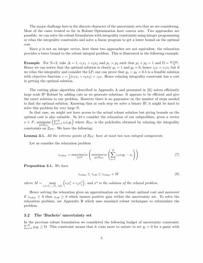
The major challenge here is the discrete character of the uncertainty sets that we are considering.Most of the cases treated so far in Robust Optimization have convex sets. Two approaches arepossible: we can solve the robust formulation with integrality constraints using integer programmingor relax the integrality constraints and solve a linear program to get a lower bound on the optimalcost.

Since p is not an integer vector, here these two approaches are not equivalent, the relaxationprovides a lower bound to the robust integral problem. This is illustrated in the following example.

Example For N=2, take ∆ = 1, c1x1 > c2x2 and p1 > p2 such that p1 + p2 = 1 and Ω = p1+p22 .

Hence we can notice that the optimal solution is clearly y1 = 1 and y2 = 0, hence zIP = c1x1 but ifwe relax the integrality and consider the LP, one can prove that y1 = y2 = 0.5 is a feasible solutionwith objective function z = 1

2(c1x1 + c2x2) < zIP . Hence relaxing integrality constraint has a costin getting the optimal solution.

The cutting plane algorithm (described in Appendix A and presented in [8]) solves efficientlylarge scale IP Robust by adding cuts as we generate solutions. It appears to be efficient and givethe exact solution to our problem. However there is no guarantee on the number of steps neededto find the optimal solution. Knowing that at each step we solve a binary IP, it might be hard tosolve this problem for very large N.

In that case, we might not have access to the actual robust solution but giving bounds on theoptimal cost is also valuable. So let’s consider the relaxation of our subproblem, given a vector

x ∈ P , minimizey∈RPC

(∑Ni=1 cixiyi

)where RPC is the polyhedra obtained by relaxing the integrality

constraints on ΞPC . We have the following:

Lemma 3.1. All the extreme points of RPC have at most two non integral components

Let us consider the relaxation problem

zrelax = maximizex∈P

(minimize

y∈RPC

(N∑i=1

cixiyi − xi

))(7)

Proposition 3.1. We have

zrelax ≤ zrob ≤ zrelax +M (8)

where M = maxi,j=1,...,N, i 6=j

(cix∗i + cjx

∗j

), and x* is the solution of the relaxed problem.

Hence solving the relaxation gives an approximation on the robust optimal cost and moreoverif zrelax ≥ 0 then zrob ≥ 0 which insures positive gain within the uncertainty set. To solve therelaxation problem, see Appendix B which uses standard robust techniques to reformulate theproblem.

3.2 The ‘Buckets’ uncertainty set

In the previous robust formulation we considered the following budget of uncertainty constraint:∑Ni=1 piyi ≥ Ω. This constraint means that it costs more to nature to set yi = 0 for a game with

5

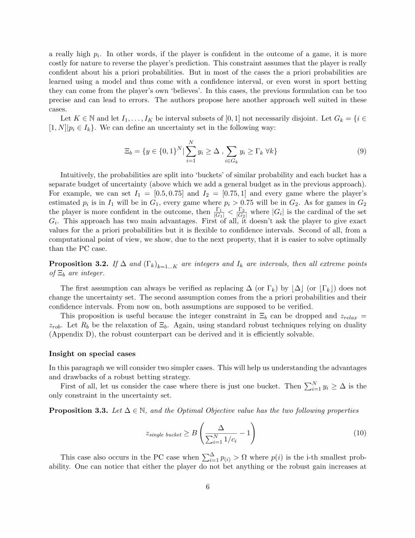
a really high pi. In other words, if the player is confident in the outcome of a game, it is morecostly for nature to reverse the player’s prediction. This constraint assumes that the player is reallyconfident about his a priori probabilities. But in most of the cases the a priori probabilities arelearned using a model and thus come with a confidence interval, or even worst in sport bettingthey can come from the player’s own ‘believes’. In this cases, the previous formulation can be tooprecise and can lead to errors. The authors propose here another approach well suited in thesecases.

Let K ∈ N and let I1, . . . , IK be interval subsets of [0, 1] not necessarily disjoint. Let Gk = i ∈[1, N ]|pi ∈ Ik. We can define an uncertainty set in the following way:

Ξb = y ∈ 0, 1N |N∑i=1

yi ≥ ∆ ,∑i∈Gk

yi ≥ Γk ∀k (9)

Intuitively, the probabilities are split into ‘buckets’ of similar probability and each bucket has aseparate budget of uncertainty (above which we add a general budget as in the previous approach).For example, we can set I1 = [0.5, 0.75] and I2 = [0.75, 1] and every game where the player’sestimated pi is in I1 will be in G1, every game where pi > 0.75 will be in G2. As for games in G2

the player is more confident in the outcome, then Γ1|G1| <

Γ2|G2| where |Gi| is the cardinal of the set

Gi. This approach has two main advantages. First of all, it doesn’t ask the player to give exactvalues for the a priori probabilities but it is flexible to confidence intervals. Second of all, from acomputational point of view, we show, due to the next property, that it is easier to solve optimallythan the PC case.

Proposition 3.2. If ∆ and (Γk)k=1...K are integers and Ik are intervals, then all extreme pointsof Ξb are integer.

The first assumption can always be verified as replacing ∆ (or Γk) by b∆c (or bΓkc) does notchange the uncertainty set. The second assumption comes from the a priori probabilities and theirconfidence intervals. From now on, both assumptions are supposed to be verified.

This proposition is useful because the integer constraint in Ξb can be dropped and zrelax =zrob. Let Rb be the relaxation of Ξb. Again, using standard robust techniques relying on duality(Appendix D), the robust counterpart can be derived and it is efficiently solvable.

Insight on special cases

In this paragraph we will consider two simpler cases. This will help us understanding the advantagesand drawbacks of a robust betting strategy.

First of all, let us consider the case where there is just one bucket. Then∑N

i=1 yi ≥ ∆ is theonly constraint in the uncertainty set.

Proposition 3.3. Let ∆ ∈ N, and the Optimal Objective value has the two following properties

zsingle bucket ≥ B

(∆∑N

i=1 1/ci− 1

)(10)

This case also occurs in the PC case when∑∆

i=1 p(i) > Ω where p(i) is the i-th smallest prob-ability. One can notice that either the player do not bet anything or the robust gain increases at

6

least linearly in the budget and in the ratio between ∆/N and 1N

∑Ni=1 1/ci. This ratio, called the

‘edge ratio’ represents the overall edge of the player on the bookmakers, which is different from thegame to game edge normally assumed in the literature. The results shows that a positive gameby game ratio is better but not a necessary assumption in the study of betting. It is important tounderstand that ∆ represents two features of the probabilities: ∆ is large not only when the playerhas an edge but also when he is confident about this edge.

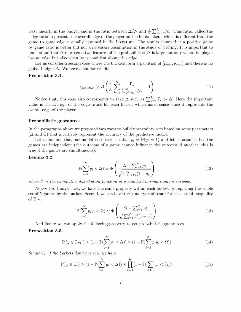
Let us consider a second case where the buckets form a partition of [pmin, pmax] and there is noglobal budget ∆. We have a similar result:

Proposition 3.4.

zpartition ≥ B

(1

K

K∑k=1

Γk∑Nj∈Gk

1/cj− 1

)(11)

Notice that, this case also corresponds to take ∆ such as∑K

k=1 Γk > ∆. Here the importantvalue is the average of the edge ratios for each bucket which make sense since it represents theoverall edge of the player.

Probabilistic guarantees

In the paragraphs above we proposed two ways to build uncertainty sets based on some parameters(∆ and Ω) that intuitively represent the accuracy of the predictive model.

Let us assume that our model is correct, i.e that pi = P(yi = 1) and let us assume that thegames are independent (the outcome of a game cannot influence the outcome if another, this istrue if the games are simultaneous).

Lemma 3.2.

P(N∑i=1

yi < ∆) ' Φ

∆−∑N

i=1 pi√∑Ni=1 pi(1− pi)

(12)

where Φ is the cumulative distribution function of a standard normal random variable.

Notice two things: first, we have the same property within each bucket by replacing the wholeset of N games by the bucket. Second, we can have the same type of result for the second inequalityof ΞPC .

P(

N∑i=1

piyi < Ω) ' Φ

Ω−∑N

i=1 p2i√∑N

i=1 p3i (1− pi)

(13)

And finally we can apply the following property to get probabilistic guarantees.

Proposition 3.5.

P (y ∈ ΞPC) ≥ (1− P(N∑i=1

yi < ∆))× (1− P(N∑i=1

piyi < Ω)) (14)

Similarly, if the buckets don’t overlap, we have

P (y ∈ Ξb) ≥ (1− P(

N∑i=1

yi < ∆))×K∏k=1

(1− P(∑i∈Gk

yi < Γk)) (15)

7

4 Simulations

This section has two main goals. First, we want to illustrate the trade off between ‘high worst casereturn’ and probabilistic guarantee and thus provide an approach to select the appropriate valuesfor the parameters (∆,Γ,Ω). Secondly, we want to compare the performances of robust strategiesto other stochastic optimization approaches.

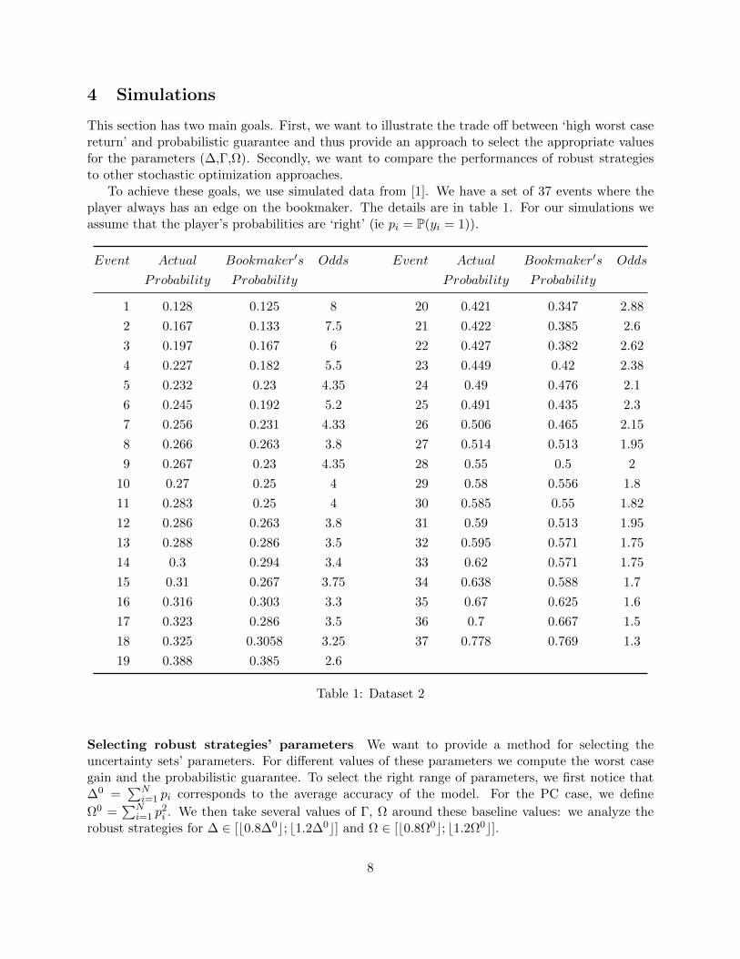
To achieve these goals, we use simulated data from [1]. We have a set of 37 events where theplayer always has an edge on the bookmaker. The details are in table 1. For our simulations weassume that the player’s probabilities are ‘right’ (ie pi = P(yi = 1)).

Event Actual Bookmaker′s Odds Event Actual Bookmaker′s Odds

Probability Probability Probability Probability

1 0.128 0.125 8 20 0.421 0.347 2.88

2 0.167 0.133 7.5 21 0.422 0.385 2.6

3 0.197 0.167 6 22 0.427 0.382 2.62

4 0.227 0.182 5.5 23 0.449 0.42 2.38

5 0.232 0.23 4.35 24 0.49 0.476 2.1

6 0.245 0.192 5.2 25 0.491 0.435 2.3

7 0.256 0.231 4.33 26 0.506 0.465 2.15

8 0.266 0.263 3.8 27 0.514 0.513 1.95

9 0.267 0.23 4.35 28 0.55 0.5 2

10 0.27 0.25 4 29 0.58 0.556 1.8

11 0.283 0.25 4 30 0.585 0.55 1.82

12 0.286 0.263 3.8 31 0.59 0.513 1.95

13 0.288 0.286 3.5 32 0.595 0.571 1.75

14 0.3 0.294 3.4 33 0.62 0.571 1.75

15 0.31 0.267 3.75 34 0.638 0.588 1.7

16 0.316 0.303 3.3 35 0.67 0.625 1.6

17 0.323 0.286 3.5 36 0.7 0.667 1.5

18 0.325 0.3058 3.25 37 0.778 0.769 1.3

19 0.388 0.385 2.6

Table 1: Dataset 2

Selecting robust strategies’ parameters We want to provide a method for selecting theuncertainty sets’ parameters. For different values of these parameters we compute the worst casegain and the probabilistic guarantee. To select the right range of parameters, we first notice that∆0 =

∑Ni=1 pi corresponds to the average accuracy of the model. For the PC case, we define

Ω0 =∑N

i=1 p2i . We then take several values of Γ, Ω around these baseline values: we analyze the

robust strategies for ∆ ∈ [b0.8∆0c; b1.2∆0c] and Ω ∈ [b0.8Ω0c; b1.2Ω0c].

8

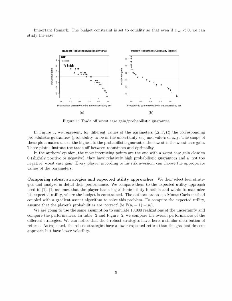
Important Remark: The budget constraint is set to equality so that even if zrob < 0, we canstudy the case.

0.0 0.2 0.4 0.6 0.8 1.0

−30

−20

−10

010

2030

Tradeoff Robustness/Optimality (PC)

Probabilistic guarantee to be in the uncertainty set

wor

st c

ase

gain

(a)

0.0 0.2 0.4 0.6 0.8

−40

−20

020

4060

Tradeoff Robustness/Optimality (bucket)

Probabilistic guarantee to be in the uncertainty set

wor

st c

ase

gain

(b)

Figure 1: Trade off worst case gain/probabilistic guarantee

In Figure 1, we represent, for different values of the parameters (∆,Γ,Ω) the correspondingprobabilistic guarantees (probability to be in the uncertainty set) and values of zrob. The shape ofthese plots makes sense: the highest is the probabilistic guarantee the lowest is the worst case gain.These plots illustrate the trade off between robustness and optimality.

In the authors’ opinion, the most interesting points are the one with a worst case gain close to0 (slightly positive or negative), they have relatively high probabilistic guarantees and a ‘not toonegative’ worst case gain. Every player, according to his risk aversion, can choose the appropriatevalues of the parameters.

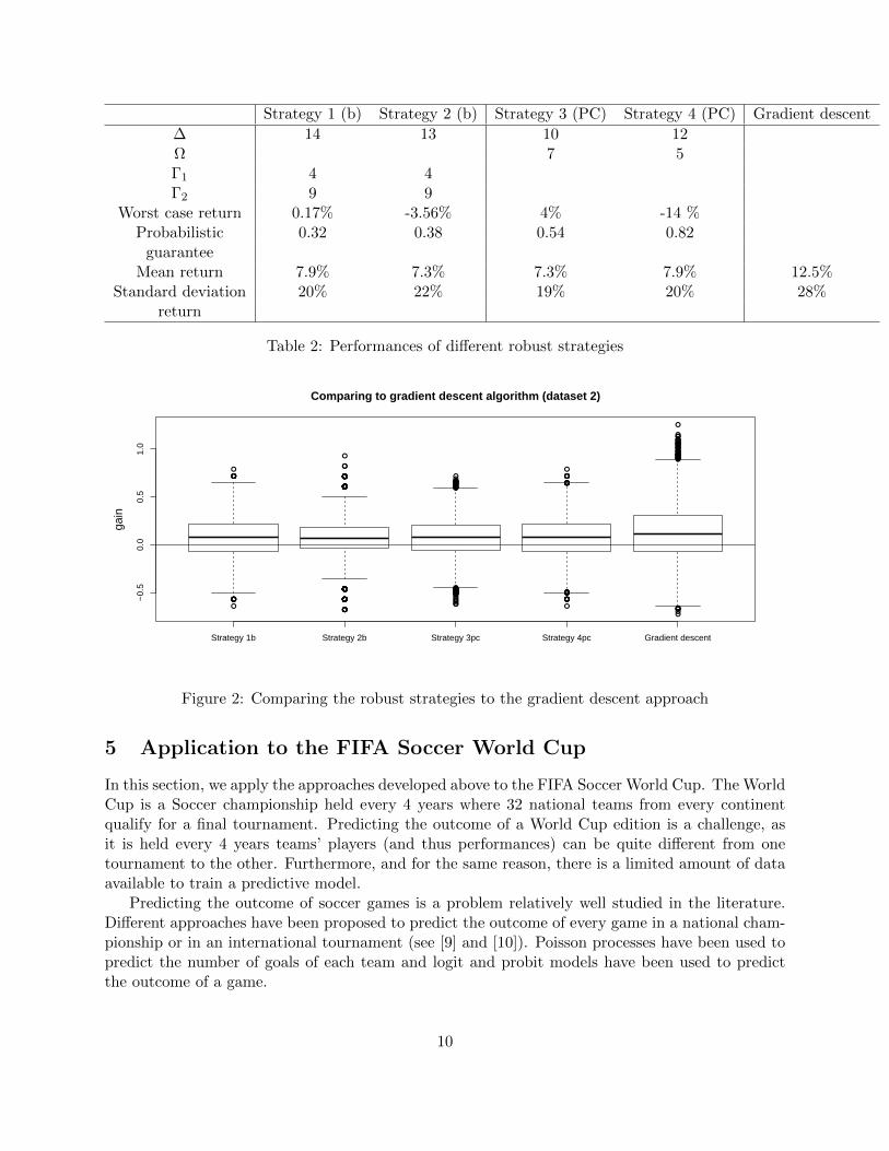
Comparing robust strategies and expected utility approaches We then select four strate-gies and analyze in detail their performance. We compare them to the expected utility approachused in [1]. [1] assumes that the player has a logarithmic utility function and wants to maximizehis expected utility, where the budget is constrained. The authors propose a Monte Carlo methodcoupled with a gradient ascent algorithm to solve this problem. To compute the expected utility,assume that the player’s probabilities are ‘correct’ (ie P(yi = 1) = pi).

We are going to use the same assumption to simulate 10,000 realizations of the uncertainty andcompare the performances. In table 2 and Figure 2, we compare the overall performances of thedifferent strategies. We can notice that the 4 robust strategies have, here, a similar distribution ofreturns. As expected, the robust strategies have a lower expected return than the gradient descentapproach but have lower volatility.

9

Strategy 1 (b) Strategy 2 (b) Strategy 3 (PC) Strategy 4 (PC) Gradient descent

∆ 14 13 10 12Ω 7 5Γ1 4 4Γ2 9 9

Worst case return 0.17% -3.56% 4% -14 %Probabilistic 0.32 0.38 0.54 0.82

guaranteeMean return 7.9% 7.3% 7.3% 7.9% 12.5%

Standard deviation 20% 22% 19% 20% 28%return

Table 2: Performances of different robust strategies

Strategy 1b Strategy 2b Strategy 3pc Strategy 4pc Gradient descent

−0.

50.

00.

51.

0

Comparing to gradient descent algorithm (dataset 2)

gain

Figure 2: Comparing the robust strategies to the gradient descent approach

5 Application to the FIFA Soccer World Cup

In this section, we apply the approaches developed above to the FIFA Soccer World Cup. The WorldCup is a Soccer championship held every 4 years where 32 national teams from every continentqualify for a final tournament. Predicting the outcome of a World Cup edition is a challenge, asit is held every 4 years teams’ players (and thus performances) can be quite different from onetournament to the other. Furthermore, and for the same reason, there is a limited amount of dataavailable to train a predictive model.

Predicting the outcome of soccer games is a problem relatively well studied in the literature.Different approaches have been proposed to predict the outcome of every game in a national cham-pionship or in an international tournament (see [9] and [10]). Poisson processes have been used topredict the number of goals of each team and logit and probit models have been used to predictthe outcome of a game.

10

Entire Data Set Restricted Data Set

Accuracy Accuracy

Train Baseline 33% Train Baseline 33%

Train Model 38% Train Model 57%

Test Baseline 33% Test Baseline 33%

Test Model 50% Test Model 52%

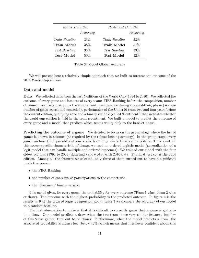
Table 3: Model Global Accuracy

We will present here a relatively simple approach that we built to forecast the outcome of the2014 World Cup edition.

Data and model

Data We collected data from the last 5 editions of the World Cup (1994 to 2010). We collected theoutcome of every game and features of every team: FIFA Ranking before the competition, numberof consecutive participation to the tournament, performance during the qualifying phase (averagenumber of goals scored and conceded), performance of the Under20 team two and four years beforethe current edition, qualifying zone and a binary variable (called ‘Continent’) that indicates whetherthe world cup edition is held in the team’s continent. We built a model to predict the outcome ofevery game and a model that predicts which teams will qualify to the bracket phase.

Predicting the outcome of a game We decided to focus on the group stage where the list ofgames is known in advance (as required by the robust betting strategy). In the group stage, everygame can have three possible outcomes: one team may win or there can be a draw. To account forthis soccer-specific characteristic of draws, we used an ordered logistic model (generalization of alogit model that can handle multiple and ordered outcomes). We trained our model with the fouroldest editions (1994 to 2006) data and validated it with 2010 data. The final test set is the 2014edition. Among all the features we selected, only three of them turned out to have a significantpredictive power:

• the FIFA Ranking

• the number of consecutive participations to the competition

• the ‘Continent’ binary variable

This model gives, for every game, the probability for every outcome (Team 1 wins, Team 2 winsor draw). The outcome with the highest probability is the predicted outcome. In figure 4 is theresults in R of the ordered logistic regression and in table 3 we compare the accuracy of our modelto a random baseline.

The first observation to make is that it is difficult to correctly guess that a game is going tobe a draw. Our model predicts a draw when the two teams have very similar features, but fewof this ‘close games’ turn out to be draws. Furthermore, when the model predicts a draw, theassociated probability is always low (below 40%) which means that it is never confident about this

11

Train Test

Accuracy Accuracy

Baseline 50% Baseline 50%

Smart Baseline 72.9% Smart Baseline 65.6%

Model 75.7% Test Model 68.7%

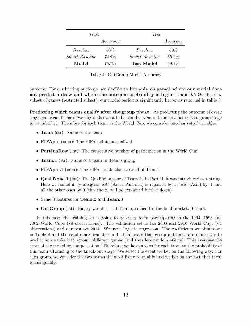
Table 4: OutGroup Model Accuracy

outcome. For our betting purposes, we decide to bet only on games where our model doesnot predict a draw and where the outcome probability is higher than 0.5 On this newsubset of games (restricted subset), our model performs significantly better as reported in table 3.

Predicting which teams qualify after the group phase As predicting the outcome of everysingle game can be hard, we might also want to bet on the event of team advancing from group stageto round of 16. Therefore for each team in the World Cup, we consider another set of variables:

• Team (str): Name of the team

• FIFApts (num): The FIFA points normalized

• PartInaRow (int): The consecutive number of participation in the World Cup

• Team.1 (str): Name of a team in Team’s group

• FIFApts.1 (num): The FIFA points also rescaled of Team.1

• Qualifzone.1 (int): The Qualifying zone of Team.1. In Part II, it was introduced as a string.Here we model it by integers; ‘SA’ (South America) is replaced by 1, ‘AS’ (Asia) by -1 andall the other ones by 0 (this choice will be explained further down)

• Same 3 features for Team.2 and Team.3

• OutGroup (int): Binary variable. 1 if Team qualified for the final bracket, 0 if not.

In this case, the training set is going to be every team participating in the 1994, 1998 and2002 World Cups (88 observations). The validation set is the 2006 and 2010 World Cups (64observations) and our test set 2014. We use a logistic regression. The coefficients we obtain arein Table 8 and the results are available in 4. It appears that group outcomes are more easy topredict as we take into account different games (and thus less random effects). This averages theerror of the model by compensation. Therefore, we have access for each team to the probability ofthis team advancing to the knock-out stage. We select the event we bet on the following way: Foreach group, we consider the two teams the most likely to qualify and we bet on the fact that theseteams qualify.

12

Robust betting strategy for 2014 Applying those two models to the 2014 World Cup whichtook place this summer in Brazil, we have access to a list of N=14 events of two types: gamesand teams advancing to the next stage. Each game considered has an edge (pici > 1). With thesame methods presented in section 4, we select our parameters for both policies. After analysis, weselected the following strategy:

• The PC Approach using ∆ = 9 and Ω = 6 with zrob = 9.78 and P(y ∈ ΞPC) ≥ 80%

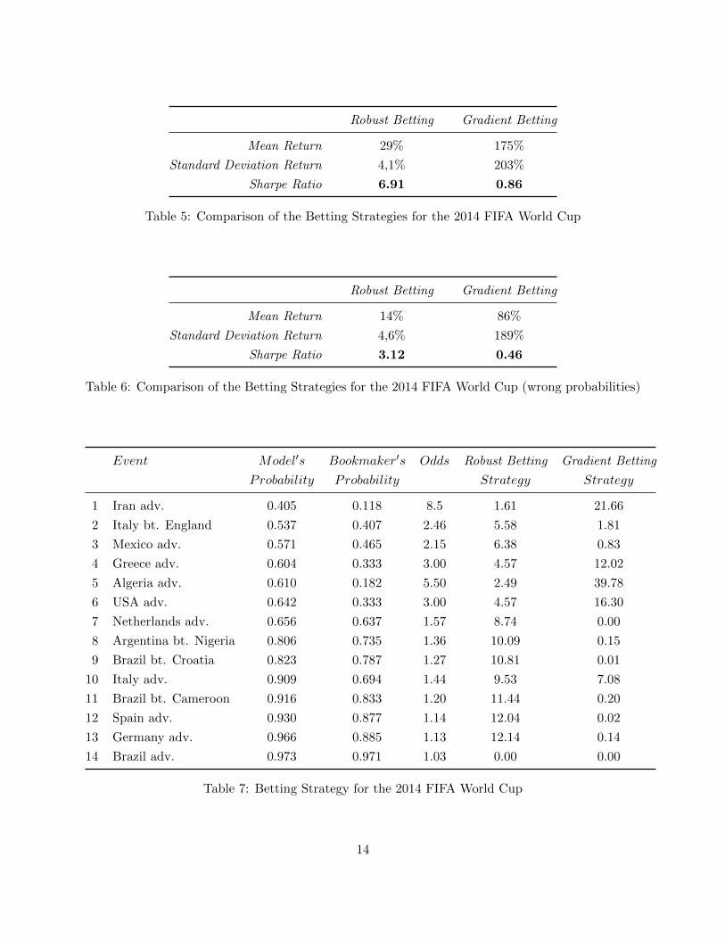
Let us compare our strategy with the one given by the gradient method. Both strategies aregiven in table 7. First of all, let us compare qualitatively the two approaches. The gradientapproach trusts the model in the sense that, the more the player has an edge, the more it bets.This seems very risky, as more than 75% of the budget is distributed on only 3 events (where theedge is important). On the opposite, the robust strategy still bets on those events as the reward isimportant but also considers the other games to diversify its risk. On the other hand, the expectedgain seems higher in the gradient strategy than in the robust one. We can verify it quantitatively.

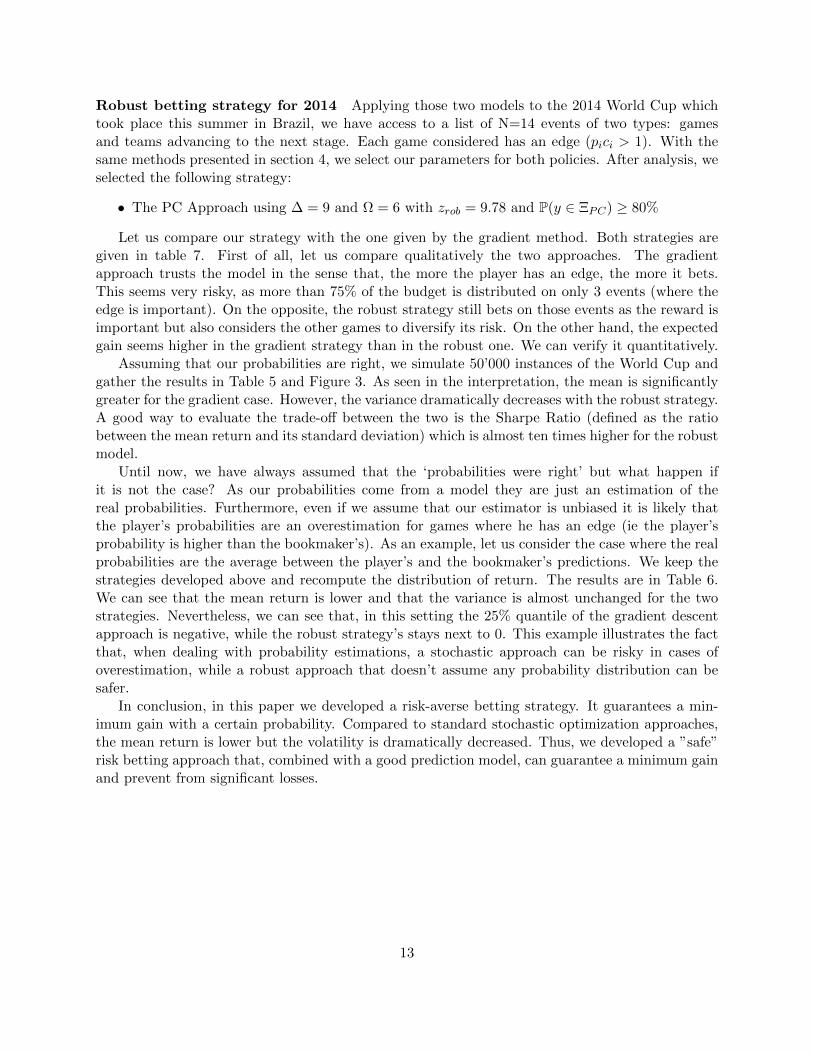
Assuming that our probabilities are right, we simulate 50’000 instances of the World Cup andgather the results in Table 5 and Figure 3. As seen in the interpretation, the mean is significantlygreater for the gradient case. However, the variance dramatically decreases with the robust strategy.A good way to evaluate the trade-off between the two is the Sharpe Ratio (defined as the ratiobetween the mean return and its standard deviation) which is almost ten times higher for the robustmodel.

Until now, we have always assumed that the ‘probabilities were right’ but what happen ifit is not the case? As our probabilities come from a model they are just an estimation of thereal probabilities. Furthermore, even if we assume that our estimator is unbiased it is likely thatthe player’s probabilities are an overestimation for games where he has an edge (ie the player’sprobability is higher than the bookmaker’s). As an example, let us consider the case where the realprobabilities are the average between the player’s and the bookmaker’s predictions. We keep thestrategies developed above and recompute the distribution of return. The results are in Table 6.We can see that the mean return is lower and that the variance is almost unchanged for the twostrategies. Nevertheless, we can see that, in this setting the 25% quantile of the gradient descentapproach is negative, while the robust strategy’s stays next to 0. This example illustrates the factthat, when dealing with probability estimations, a stochastic approach can be risky in cases ofoverestimation, while a robust approach that doesn’t assume any probability distribution can besafer.

In conclusion, in this paper we developed a risk-averse betting strategy. It guarantees a min-imum gain with a certain probability. Compared to standard stochastic optimization approaches,the mean return is lower but the volatility is dramatically decreased. Thus, we developed a ”safe”risk betting approach that, combined with a good prediction model, can guarantee a minimum gainand prevent from significant losses.

13

Robust Betting Gradient Betting

Mean Return 29% 175%

Standard Deviation Return 4,1% 203%

Sharpe Ratio 6.91 0.86

Table 5: Comparison of the Betting Strategies for the 2014 FIFA World Cup

Robust Betting Gradient Betting

Mean Return 14% 86%

Standard Deviation Return 4,6% 189%

Sharpe Ratio 3.12 0.46

Table 6: Comparison of the Betting Strategies for the 2014 FIFA World Cup (wrong probabilities)

Event Model′s Bookmaker′s Odds Robust Betting Gradient Betting

Probability Probability Strategy Strategy

1 Iran adv. 0.405 0.118 8.5 1.61 21.66

2 Italy bt. England 0.537 0.407 2.46 5.58 1.81

3 Mexico adv. 0.571 0.465 2.15 6.38 0.83

4 Greece adv. 0.604 0.333 3.00 4.57 12.02

5 Algeria adv. 0.610 0.182 5.50 2.49 39.78

6 USA adv. 0.642 0.333 3.00 4.57 16.30

7 Netherlands adv. 0.656 0.637 1.57 8.74 0.00

8 Argentina bt. Nigeria 0.806 0.735 1.36 10.09 0.15

9 Brazil bt. Croatia 0.823 0.787 1.27 10.81 0.01

10 Italy adv. 0.909 0.694 1.44 9.53 7.08

11 Brazil bt. Cameroon 0.916 0.833 1.20 11.44 0.20

12 Spain adv. 0.930 0.877 1.14 12.04 0.02

13 Germany adv. 0.966 0.885 1.13 12.14 0.14

14 Brazil adv. 0.973 0.971 1.03 0.00 0.00

Table 7: Betting Strategy for the 2014 FIFA World Cup

14

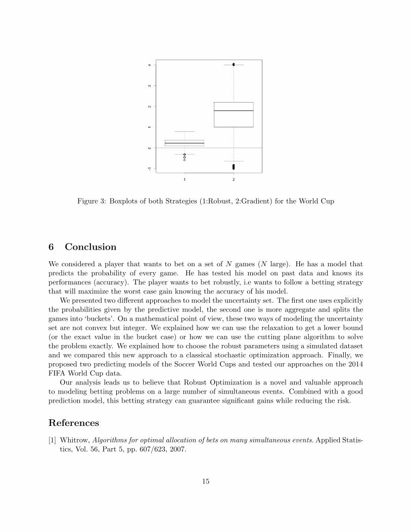
Figure 3: Boxplots of both Strategies (1:Robust, 2:Gradient) for the World Cup

6 Conclusion

We considered a player that wants to bet on a set of N games (N large). He has a model thatpredicts the probability of every game. He has tested his model on past data and knows itsperformances (accuracy). The player wants to bet robustly, i.e wants to follow a betting strategythat will maximize the worst case gain knowing the accuracy of his model.

We presented two different approaches to model the uncertainty set. The first one uses explicitlythe probabilities given by the predictive model, the second one is more aggregate and splits thegames into ‘buckets’. On a mathematical point of view, these two ways of modeling the uncertaintyset are not convex but integer. We explained how we can use the relaxation to get a lower bound(or the exact value in the bucket case) or how we can use the cutting plane algorithm to solvethe problem exactly. We explained how to choose the robust parameters using a simulated datasetand we compared this new approach to a classical stochastic optimization approach. Finally, weproposed two predicting models of the Soccer World Cups and tested our approaches on the 2014FIFA World Cup data.

Our analysis leads us to believe that Robust Optimization is a novel and valuable approachto modeling betting problems on a large number of simultaneous events. Combined with a goodprediction model, this betting strategy can guarantee significant gains while reducing the risk.

References

[1] Whitrow, Algorithms for optimal allocation of bets on many simultaneous events. Applied Statis-tics, Vol. 56, Part 5, pp. 607/623, 2007.

15

[2] Browne & Ward Whitt, Portfolio Choice and the Bayesian Kelly Criterion. Advances in AppliedProbability, Vol. 28, No. 4, pp. 1145/1176, 1996.

[3] Haigh, The Kelly Criterion and Bet Comparisons in Spread Betting. Journal of the RoyalStatistical Society, Series D, The Statistician, Vol.49, No. 4, pp. 531/539, 2000.

[4] Thorp, The Kelly criterion in blackjack, sports betting and the stock market. Edward O. Thorp& Associates, Newport Beach, 1997.

[5] Bertsimas & Sim, The Price of Robustness. Operations Research, Vol. 52, pp. 35/53, 2004.

[6] Bertsimas, Pachamanova & Sim, Robust linear optimization under general norms. OperationsResearch Letters, Vol. 32, pp. 510/516, 2004.

[7] Bertsimas, Brown & Caramanis, Theory and Applications of Robust Optimization. Society forIndustrial and Applied Mathematics, Vol. 53, No. 3, pp. 464/501, 2011.

[8] Bertsimas, Dunning & Lubin, Reformulations versus cutting planes for robust optimization, Acomputational and machine learning perspective. Working paper.

[9] Dyte & Clark, A Ratings Based Poisson Model for World Cup Soccer Simulation. The Journalof the Operational Research Society, Vol. 51, No. 8, pp. 993/998,Aug. 2000.

[10] Goddard, Regression models for forecasting goals and match results in association football.International Journal of Forecasting 21, pp.331/340, 2005.

16

Appendices

A The Robust Cutting Plane algorithm

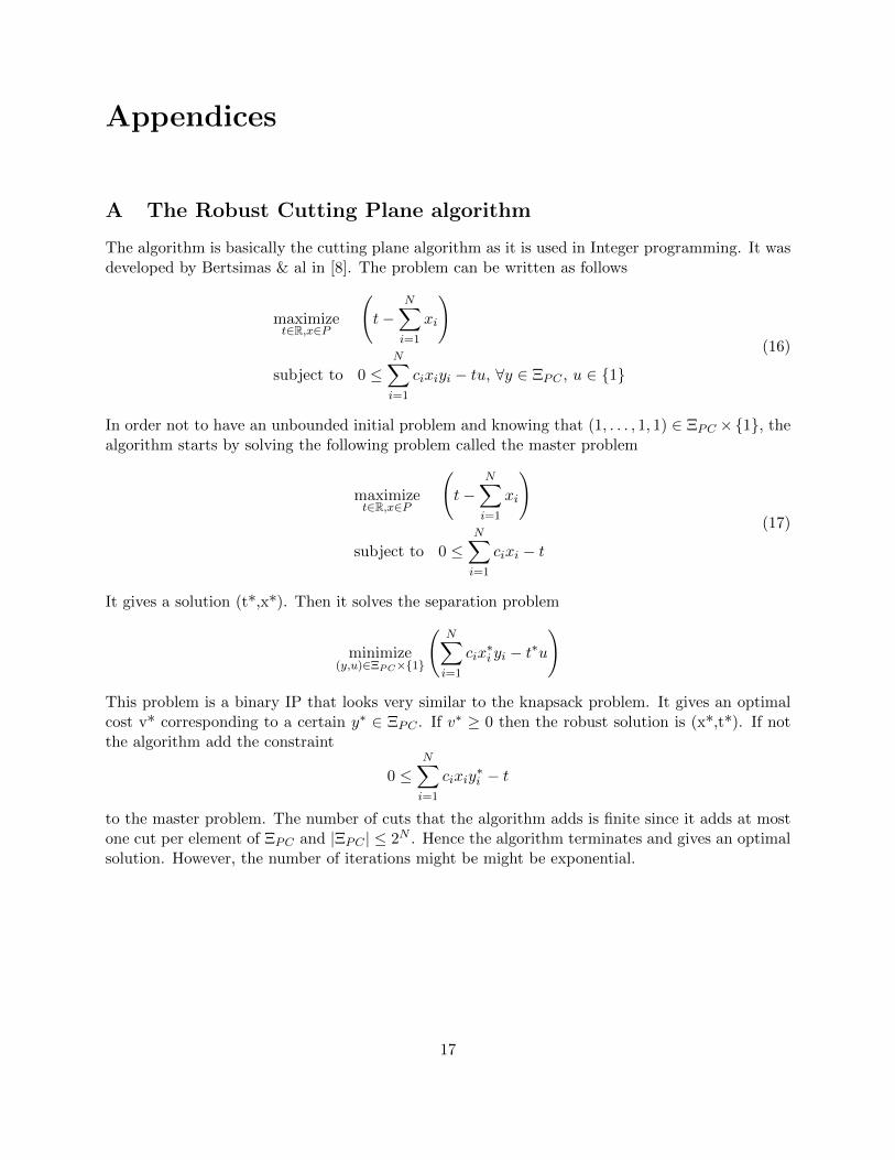
The algorithm is basically the cutting plane algorithm as it is used in Integer programming. It wasdeveloped by Bertsimas & al in [8]. The problem can be written as follows

maximizet∈R,x∈P

(t−

N∑i=1

xi

)

subject to 0 ≤N∑i=1

cixiyi − tu, ∀y ∈ ΞPC , u ∈ 1

(16)

In order not to have an unbounded initial problem and knowing that (1, . . . , 1, 1) ∈ ΞPC ×1, thealgorithm starts by solving the following problem called the master problem

maximizet∈R,x∈P

(t−

N∑i=1

xi

)

subject to 0 ≤N∑i=1

cixi − t

(17)

It gives a solution (t*,x*). Then it solves the separation problem

minimize(y,u)∈ΞPC×1

(N∑i=1

cix∗i yi − t∗u

)

This problem is a binary IP that looks very similar to the knapsack problem. It gives an optimalcost v* corresponding to a certain y∗ ∈ ΞPC . If v∗ ≥ 0 then the robust solution is (x*,t*). If notthe algorithm add the constraint

0 ≤N∑i=1

cixiy∗i − t

to the master problem. The number of cuts that the algorithm adds is finite since it adds at mostone cut per element of ΞPC and |ΞPC | ≤ 2N . Hence the algorithm terminates and gives an optimalsolution. However, the number of iterations might be might be exponential.

17

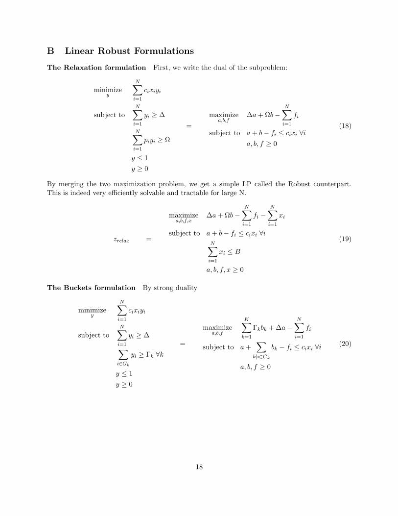
B Linear Robust Formulations

The Relaxation formulation First, we write the dual of the subproblem:

minimizey

N∑i=1

cixiyi

subject to

N∑i=1

yi ≥ ∆

N∑i=1

piyi ≥ Ω

y ≤ 1

y ≥ 0

=

maximizea,b,f

∆a+ Ωb−N∑i=1

fi

subject to a+ b− fi ≤ cixi ∀ia, b, f ≥ 0

(18)

By merging the two maximization problem, we get a simple LP called the Robust counterpart.This is indeed very efficiently solvable and tractable for large N.

zrelax =

maximizea,b,f,x

∆a+ Ωb−N∑i=1

fi −N∑i=1

xi

subject to a+ b− fi ≤ cixi ∀iN∑i=1

xi ≤ B

a, b, f, x ≥ 0

(19)

The Buckets formulation By strong duality

minimizey

N∑i=1

cixiyi

subject to

N∑i=1

yi ≥ ∆∑i∈Gk

yi ≥ Γk ∀k

y ≤ 1

y ≥ 0

=

maximizea,b,f

K∑k=1

Γkbk + ∆a−N∑i=1

fi

subject to a+∑

k|i∈Gk

bk − fi ≤ cixi ∀i

a, b, f ≥ 0

(20)

18

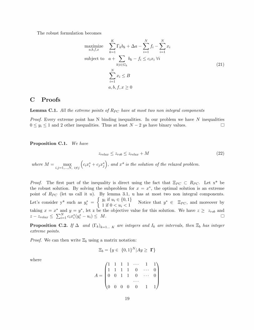
The robust formulation becomes

maximizea,b,f,x

K∑k=1

Γkbk + ∆a−N∑i=1

fi −N∑i=1

xi

subject to a+∑

k|i∈Gk

bk − fi ≤ cixi ∀i

N∑i=1

xi ≤ B

a, b, f, x ≥ 0

(21)

C Proofs

Lemma C.1. All the extreme points of RPC have at most two non integral components

Proof. Every extreme point has N binding inequalities. In our problem we have N inequalities0 ≤ yi ≤ 1 and 2 other inequalities. Thus at least N − 2 ys have binary values.

Proposition C.1. We have

zrelax ≤ zrob ≤ zrelax +M (22)

where M = maxi,j=1,...,N, i 6=j

(cix∗i + cjx

∗j

), and x* is the solution of the relaxed problem.

Proof. The first part of the inequality is direct using the fact that ΞPC ⊂ RPC . Let x* bethe robust solution. By solving the subproblem for x = x∗, the optimal solution is an extremepoint of RPC (let us call it u). By lemma 3.1, u has at most two non integral components.

Let’s consider y* such as y∗i =

yi if ui ∈ 0, 11 if 0 < ui < 1

Notice that y∗ ∈ ΞPC , and moreover by

taking x = x∗ and y = y∗, let z be the objective value for this solution. We have z ≥ zrob andz − zrelax ≤

∑Ni=1 cix

∗i (y∗i − ui) ≤ M .

Proposition C.2. If ∆ and (Γk)k=1... K are integers and Ik are intervals, then Ξb has integerextreme points.

Proof. We can then write Ξb using a matrix notation:

Ξb = y ∈ 0, 1N |Ay ≥ Γ

where

A =

1 1 1 1 · · · 1 11 1 1 1 0 · · · 00 0 1 1 0 · · · 0

· · ·0 0 0 0 0 1 1

19

and

Γ =

∆Γ1

. . .ΓK

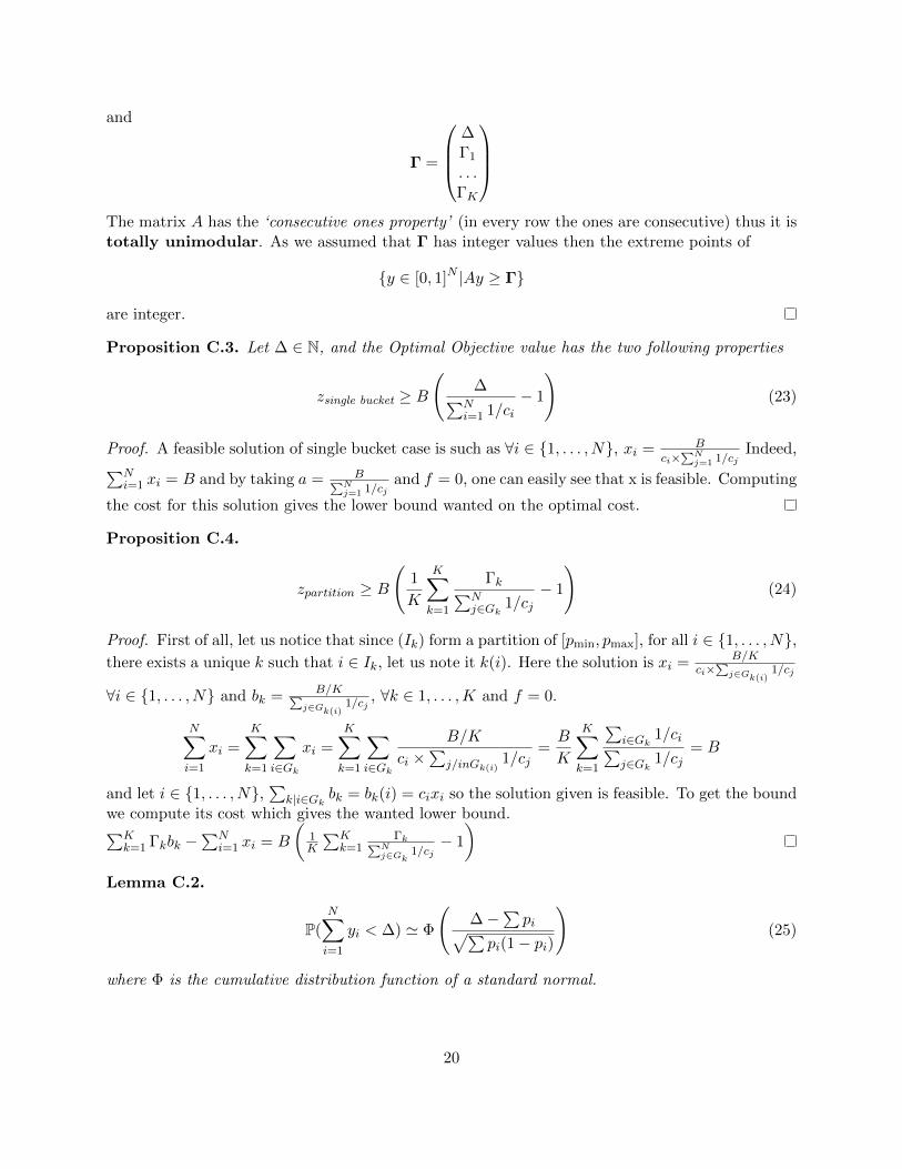
The matrix A has the ‘consecutive ones property’ (in every row the ones are consecutive) thus it istotally unimodular. As we assumed that Γ has integer values then the extreme points of

y ∈ [0, 1]N |Ay ≥ Γ

are integer.

Proposition C.3. Let ∆ ∈ N, and the Optimal Objective value has the two following properties

zsingle bucket ≥ B

(∆∑N

i=1 1/ci− 1

)(23)

Proof. A feasible solution of single bucket case is such as ∀i ∈ 1, . . . , N, xi = Bci×

∑Nj=1 1/cj

Indeed,∑Ni=1 xi = B and by taking a = B∑N

j=1 1/cjand f = 0, one can easily see that x is feasible. Computing

the cost for this solution gives the lower bound wanted on the optimal cost.

Proposition C.4.

zpartition ≥ B

(1

K

K∑k=1

Γk∑Nj∈Gk

1/cj− 1

)(24)

Proof. First of all, let us notice that since (Ik) form a partition of [pmin, pmax], for all i ∈ 1, . . . , N,there exists a unique k such that i ∈ Ik, let us note it k(i). Here the solution is xi = B/K

ci×∑

j∈Gk(i)1/cj

∀i ∈ 1, . . . , N and bk = B/K∑j∈Gk(i)

1/cj, ∀k ∈ 1, . . . ,K and f = 0.

N∑i=1

xi =K∑k=1

∑i∈Gk

xi =K∑k=1

∑i∈Gk

B/K

ci ×∑

j/inGk(i)1/cj

=B

K

K∑k=1

∑i∈Gk

1/ci∑j∈Gk

1/cj= B

and let i ∈ 1, . . . , N,∑

k|i∈Gkbk = bk(i) = cixi so the solution given is feasible. To get the bound

we compute its cost which gives the wanted lower bound.∑Kk=1 Γkbk −

∑Ni=1 xi = B

(1K

∑Kk=1

Γk∑Nj∈Gk

1/cj− 1

)Lemma C.2.

P(

N∑i=1

yi < ∆) ' Φ

(∆−

∑pi√∑

pi(1− pi)

)(25)

where Φ is the cumulative distribution function of a standard normal.

20

Proof. The result comes from the application of the central limit theorem for independent butnon identically distributed variables (Lindeberg-Feller thereom). Let us consider Xi = yi − pi asequence of independent random variables such that E(Xi) = 0 and E(X2

i ) = pi(1 − pi). Lets2n =

∑Ni=1 pi(1 − pi). Let us also assume that ∃pmax < 1, pmin > 0 s.t. pi ∈ [pmin, pmax]∀i. This

assumption is realistic as our data is bounded, the probabilities of our model are not too close to0 and 1. Then using Lyapunov condition and Lindeberg-Feller theorem we get∑N

i=1Xi

s2n

−→ N (0, 1) in distribution

and thus gives us the result.

Proposition C.5.

P (y ∈ ΞPC) ≥ (1− P(N∑i=1

yi < ∆))× (1− P(N∑i=1

piyi < Ω)) (26)

Similarly, if the buckets don’t overlap, we have

P (y ∈ Ξb) ≥ (1− P(

N∑i=1

yi < ∆))×K∏k=1

(1− P(∑i∈Gk

yi < Γk)) (27)

Proof. Let δ be the event ∑N

i=1 yi < ∆, ω = ∑N

i=1 piyi < Ω and ∀k = 1, . . . ,K, γk =∑

i∈Gkyi < Γk We have

P(y ∈ ΞPC) = P(δ, ω

)= P

(ω|δ)P(δ)

Now notice that P(ω|δ) ≥ P(ω) because if δ is true, then ω has more chance to be true than if wedidn’t have any information on δ. So

P(y ∈ ΞPC) ≥ P (ω)P(δ) = (1− P(ω))× (1− P(δ))

For the bucket case, notice that since the bucket are not overlapping then γk are independent.Using the same reasoning:

P(y ∈ Ξb) = P(δ,∀k γk

)= P

(δ|∀k γk

)P(∀k γk) = P

(δ|∀k γk

) K∏i=1

P(γk)

Again for a similar reason as before P(δ|∀k γk) ≥ P(δ) So

P(y ∈ Ξb) ≥ P(δ) K∏i=1

P(γk) = (1− P(δ))×K∏i=1

(1− P(γk))

21

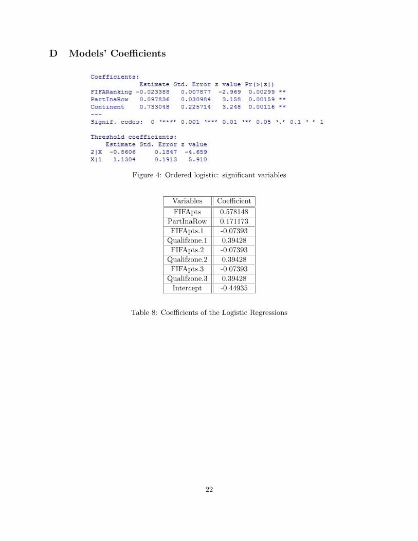
D Models’ Coefficients

Figure 4: Ordered logistic: significant variables

Variables Coefficient

FIFApts 0.578148

PartInaRow 0.171173

FIFApts.1 -0.07393

Qualifzone.1 0.39428

FIFApts.2 -0.07393

Qualifzone.2 0.39428

FIFApts.3 -0.07393

Qualifzone.3 0.39428

Intercept -0.44935

Table 8: Coefficients of the Logistic Regressions

22