Embed Size (px)
Citation preview

Risk-Return Predictions With the Fama-French Three-Factor Model Betas
Glenn Pettengill* Grand Valley State University
George Chang
Grand Valley State University
C. James Hueng Western Michigan University
Draft date: October 17, 2011
*corresponding author 616.331.7430
1
Risk-Return Predictions With the Fama-French Three-Factor Model Betas
ABSTRACT
A three-factor model regime has replaced the CAPM regime in academic research. The CAPM regime may be said to have ended with Fama and French’s (1992) finding that market beta does not predict return. Strangely, the three-factor model has not received scrutiny relative to the ability of the model to predict return and variation in return for portfolios. In this paper we test the ability of the three-factor model to predict return and return variation. We find that portfolios can be formed on the basis of the three-factor that vary with expectations in terms of risk and return. We find, however, that the CAPM performs these goals with greater efficiency. In particular expected returns for extreme portfolios are poor predictors of actual returns. Raising questions about the use of the three-factor model to risk adjust. We dissect the three-factor model’s predictive ability and find that inclusion of the systematic risk variable dealing with the book-to-market ratio distorts predictions and that a model including the market beta and the factor loading dealing with firm size seems to predict more efficiently than either the three-factor model or the CAPM.

2
I. Introduction
Modern Portfolio Theory as developed by Markowitz (1952) and others, asserts that
investors need only to assess systematic risk and may ignore idiosyncratic risk of an individual
security when creating a well-diversified portfolio. If the market is efficient, accurate modeling
and measurement of systematic risk allows for determination of expected portfolio return.
Comparisons of actual return to the expected return based on systematic risk in turn allows for
measurement of risk-adjusted return and portfolio performance. One may identify two regimes
in the academic literature for the measurement of systematic risk and subsequent measurement of
risk-adjusted returns: the Capital Asset Pricing Model (CAPM) regime, which may be dated
from the Mid 1960s through the early 1990s, and the Fama-French three-factor model (FF-3FM)
regime, which may be dated from the early 1990s through the present day.
The CAPM, as developed by Sharpe (1964), Lintner (1965) and Mossin (1966), states
that the systematic risk of a security can be determined by a single variable, the security’s
sensitivity to changes in the overall market, the security’s market beta. Although difficulties
existed with the application of the model (for example how to measure total market return),
during the CAPM regime expected return for a portfolio was measured as:
( ) ( )pt p mtE R E Rβ= ⋅ . (1)
Here the expected return of a portfolio in excess of the risk free return for a particular time
period, , is determined by the portfolio’s beta, and the expected return of the market in
excess of the risk free return for the same time period, .
( )ptE R
( )mtE R

3
The CAPM provided a straightforward means of risk-adjusting returns and measuring the
portfolio manager’s performance. Under the CAPM regime the manager sought to earn a return
in excess of the return predicted by equation (1). That is, the portfolio manager attempted to
earn a positive “alpha” as shown in equation (2):
, (2)
where the portfolio and market excess returns are the realized returns rather than the expected
returns for a given time period.
Empirical studies in support of the theoretically developed CAPM such as Black, Jensen
and Scholes (1972) and Fama and MacBeth (1973) found a positive relationship between
portfolios betas determined in estimation periods and portfolio returns in a subsequent test
periods. These results sustained the use of the CAPM during the extended regime of the model,
but two lines of research developed which ultimately ended the CAPM regime. First, the
CAPM’s claim that beta risk was the sole determinant of the expected return for a well-
diversified portfolio was challenged by the discovery of a number of anomalies. For example,
portfolios of small-firm securities and portfolios of securities with high book-to-market (BtM)
ratios were shown to earn higher returns than justified by beta risk [see for example Banz (1981)
and Rosenburg, Reid and Lanstein (1985)]. The second line of research found temporal
inconsistencies in the relationship between estimated portfolio betas and realized portfolio
returns. Reinganum (1981) found inconsistencies in the relationship between betas and returns
across years and Tinic and West (1984) found inconsistencies across months of the year,
although Pettengill, Sundaram and Mathur (1995) showed that these results followed from a
pt p p mtR Rα β= + ⋅

4
failure to distinguish between up and down markets in the test periods. These two lines of
research blended in a seminal study that saw the end of the CAPM regime.
The beginning of the end of the CAPM regime may be dated as the publication of the
landmark study, Fama and French (1992). In this study, Fama and French find that for securities
firm size and BtM ratios explain returns but beta does not. They argue that firm size and the
BtM ratio must proxy for systematic risk but that beta evidently does not. Fama and French
(1993) introduce a three-factor model, FF-3FM, which explains the returns for portfolios
examined in their study. The model they introduced has widely supplanted the CAPM in risk-
adjusting returns in academic studies and in studies published in the practitioner literature.
Because the three-factor model has become dominant in research studies we may speak of the
existence of a three-factor model regime. The FF-3FM model is specified as:
. (3)
In this model the expected return in excess of the risk-free rate for a portfolio, E(Rpt), depends on
the level of three systematic risk factors and the portfolio’s exposure to each of these factors.
The first factor (ironically given the finding that the CAPM beta does not explain returns)
duplicates the factor in the CAPM, ( , now denoted as MKT). The second factor, HML,
measures the return of a zero-investment portfolio long in securities with high BtM ratios (value
securities) and short in securities with low BtM ratios (growth securities). The third factor, SMB,
measures the return of a zero-investment portfolio long in small-firm securities and short in
large-firm securities. The factor loadings of , , and measure portfolio p’s respective
exposure to each of these systematic risk factors.
( ) ( ) ( ) ( )pt pm t ph t ps tE R E MKT E HML E SMBβ β β= ⋅ + ⋅ + ⋅
mR
pmβ phβ psβ

5
The FF-3FM model has clearly replaced the CAPM in terms of risk-adjusting in research
studies. The CAPM, however, remains the dominant model in business applications.1 And
surprisingly there has not been, as there was with the CAPM, studies of the ability of the FF-
3FM to build portfolios which produce return variation in accordance with model predictions.
This lack of study is curious as it was in large part the failure of the CAPM to meet this criterion,
according to some studies, that led to the end of the CAPM regime.
Koch and Westheide (2010) study the relationship between the FF-3FM betas and future
returns. They find that all three factors have significant predictive ability for the returns for the
twenty-five portfolios formed based on BtM and size [as created by Fama and French (1993)]
when markets are divided into up and down markets based on these factor loadings. They find,
however, that the factor loadings on SMB and MKT beta are not paid a risk premium.
Robustness tests for other portfolios formed on factors such as momentum provide additional
questions as to the predictive ability of the factor loadings of the three-factor model.
In this paper we provide a more direct test of the FF-3FM model by forming portfolios
based on estimated security returns as predicted by factor loadings and historic factor values.
We seek to determine if portfolios formed on this basis will show the risk-return profiles
predicted by the FF-3FM. For comparison purposes we include predictions based on the CAPM.
The rest of the paper proceeds as follows. In Section II, we present the methodology used to
form the portfolios based on the FF-3FM and CAPM and report results of portfolio performance.
We find that the FF-3FM and CAPM both allow the creation of portfolios which exhibit
expected risk-return profiles. Indeed the results from these two models appear to be surprisingly
1 For instance the Wall Street Prep course in their training manual asserts that among several competing asset-
pricing models, “The most popular and commonly used in practice is the capital asset pricing model (CAPM).” (p.
86) In addition, see Bartholdy and Peare (2005), Estrada (2011) and Graham and Harvey (2001).

6
similar. There are, however, difficulties with the predictions of both models. In Section III, we
dissect the FF-3FM to determine which factor loadings are essential for accurate predictions.
We find that a two-factor model including the size and market betas appears to provide superior
predictions to the FF-3FM. We present our conclusions in Section IV.
7
II. Predicting Returns and Risk: FF-3FM and CAPM
A. Methodology
For nearly two decades, the FF-3FM model has been the dominant model to risk-adjust
return in research studies. Perhaps because of the empirical nature of the FF-3FM, it has not
been subject to the same type of testing of its predictive power as was applied to the theoretical
CAPM. In this paper we build portfolios using the FF-3FM which should vary in terms of a risk-
return continuum. For comparison purposes we apply identical sampling procedures to the
CAPM, building portfolios that should likewise experience differentiation along a risk-return
continuum.
Our methodology most closely follows the seminal work of Fama and MacBeth (1973) as
applied to the CAPM. We estimate security betas in a sample period, create portfolios at the end
of the period and then monitor portfolio performance in a subsequent one-year period. We
estimate beta for securities with monthly return data available in the CRSP dataset using three-
year estimation periods. In our estimation process we include all securities available on the
CRSP tape with the exception of ETFs, Closed-End Funds and ADRs. We require that each
security included in the estimation process has at least 24 months of return data during the three-
year estimation period. For the FF-3FM we estimate three betas for security using equation (4):
(4)
and for the CAPM we estimate the single market beta using equation (5):
(5)
it im t is t ih t itR MKT SMB HMLβ β β ε= ⋅ + ⋅ + ⋅ +
it im t itR MKTβ ε= ⋅ +

8
where all variables are as defined for equations (3) and (2) except we have realized values
instead of expected values for each of the factors. In our estimation of MKT beta we use the
CRSP value-weighted index to determine market return. To determine the SMB beta and the
HML beta, we acquire the returns for the two zero-investment portfolios from Kenneth French’s
website.
At the end of each three-year period we form ten portfolios based on estimated security
betas. For the CAPM the portfolio formation follows the procedure of the Fama and MacBeth
(1973) methodology. We rank all securities based on estimated market beta placing the ten
percent of the securities with the highest beta into portfolio 1, and so on, until the 10% of the
securities with the lowest betas are placed into portfolio 10. The CAPM predicts that Portfolio 1
should enjoy the highest realized return at the cost of the highest realized risk. Likewise,
Portfolio 10 should enjoy the lowest realized risk at the cost of the lowest realized return.
We follow portfolio formation in the same spirit of the Fama and MacBeth (1973)
procedure as we form portfolios for the FF-3FM. We use the same three-year estimation periods
and regress monthly security excess returns against monthly values for all three factors. Thus,
we gain three beta estimates for each security that we will jointly use to create portfolios with a
goal of producing outputs consistent with a risk-return tradeoff. When creating portfolios based
on the CAPM a single beta is used to create portfolios. When creating portfolios based on the
FF-3FM, three factor betas are used and the formation procedure cannot be a straight forward
result of beta values. The FF-3FM is an empirical rather than a theoretical model, and, as such,
does not provide a theoretical basis to combine the three betas to form total risk. Because the
three betas measure the sensitivity of a security’s return with respect to each of the three factors
whose values are distinct, it is not meaningful to simply add the three betas to determine total

9
systematic risk. We can, however, use the model to predict expected return in excess of the risk-
free return. If the risk-return tradeoff holds and the FF-3FM accurately measures risk, those
securities with the higher expected return according to the model should also have the higher
expected risk. Thus, using the observed average value from the entire sample period for each
factor we predict expected excess return2 for each security at the end of each estimation period
using equation (6).
������ = � ∗ �� ��������� +�� ∗ ������������ +�� ∗ ����������� (6)
where all variables are as defined in equation (3) except that the factor values represent average
values over the entire sample period instead of expected values.
Based on these expected returns, we place each security in one of ten portfolios. As with
the CAPM formation process, Portfolio 1 contains the securities with the highest expected return
and, by inference, the highest expected risk. Portfolio 10 contains securities with the lowest
expected return and by inference the lowest expected risk.
We hold portfolios for a one-year period including in the portfolio any security with a
reported return for any month during the holding period. We calculate the portfolio return for
each month of the one-year holding period as the equally-weighted return of all securities in the
portfolio. We use overlapping sample periods to estimate the betas and observe portfolio returns.
The portfolios are rebalanced at the beginning of each estimation period. Our first estimation
period uses data from January 1927 through December 1929. Based upon these estimates we
form portfolios that are held for the period from January 1930 through December 1930. Our
2 Notice that portfolio formation for the CAPM is also based on expected return as expected security return is
perfectly correlated with the MKT beta for the security.

10
penultimate estimation period uses data from January 2005 through December 2007. Based
upon these estimates we form portfolios that are held for the period from January 2008 through
December 2008. Our final estimation period uses data from January 2006 through December
2008. Based upon these estimates we form portfolios that are held for the period January 2009
through December 2009. There are a total of 80 such estimation (and holding) periods.
Our goal is to investigate if the FF-3FM can create portfolios with a risk-return profile
consistent with the model’s prediction and to compare the performance of the FF-3FM to the
performance of the CAPM. If these models effectively measure risk and the market rewards
investors for assuming risk, for both models Portfolio 1 should achieve the highest average
return and experience the highest risk. Portfolio 10 should experience the lowest risk at the cost
of the lowest average return. Moving across portfolios from Portfolio 1 to Portfolio 10 both
realized returns and risk should decrease monotonically.
To achieve our goal of measuring the efficiency of the model in the creating portfolios
that vary along a risk-return continuum our methodology must differ from previous studies.
Studies such as Fama and MacBeth (1973), Tinic and West (1984), and Fama and French (1992)
test the CAPM by comparing portfolio or security betas to returns. There are two reasons why
we must take a different tack on this study. First, while the CAPM allows a test between a single
beta and returns, the FF-3FM assumes a relationship between return and three betas with no
guidance as to how to combine the several betas into a single measure of risk. Second, we seek
to examine risk on an ex-post basis in which case the appropriate measure for risk becomes total
risk not systematic risk. Thus, we measure portfolio performance by computing the average
monthly return for the portfolio across the 80 sample holding periods and the standard deviation
of monthly return across the 80 sample holding periods.

11
Because the use of the standard deviation of return as a post-formation measure of risk
may strike the reader as inappropriate, we provide some additional clarification. We
acknowledge that the standard deviation of monthly returns is not an appropriate ex ante measure
of risk for a security, because only systematic risk should be considered in adding a security to a
portfolio. On an ex ante basis one might measure a security’s covariance with the market to
determine that security’s addition to total portfolio risk. We are, however, examining risk post-
portfolio formation for the entire portfolio. On this ex post basis the variation in portfolio returns
as measured by standard deviations in monthly returns is the appropriate measure of realized
risk. If we measure return performance on an ex-post basis we should do the same for portfolio
risk performance! Previous tests have, for the most part, assumed that ex ante beta risk repeats.
In their second stage of model test, Fama and MacBeth (1973) implicitly test this assumption by
examining whether the rank of portfolio betas follow the ranking of the created betas. Because
on an ex post basis the question for a portfolio manager is the total variation in the portfolio, we
directly examine risk on this basis.
B. Portfolio Performance: FF-3FM and CAPM
We have formed ten portfolios based on expected return and risk in accordance with
factor loadings on the FF-3FM. Portfolio 1 is built with securities which have the highest
expected return and expected risk according to the FF-3FM. We build nine additional portfolios
each with a lower expected return and risk based on beta loadings on the FF-3FM equation until
we create Portfolio 10 which has the lowest expected return and risk. Our goal is to test whether
measuring risk using the FF-3FM could allow a portfolio manager to reliably build portfolios
along a risk-return continuum. Results reported in Panel A of Table 1 indicate the average

12
monthly return and standard deviation of monthly return for the ten FF-3FM portfolios. These
results suggest that the FF-3FM can be used to build portfolios tailored for an investor’s risk-
return tradeoff. Portfolio 1 has the highest realized average return among the ten portfolios and
average returns generally fall across portfolios as ex ante risk falls. Likewise, Portfolio 1 has the
highest realized risk among the ten portfolios as measured by the standard deviation in monthly
returns. Thus ex post risk generally falls across portfolios as predicted by the declining ex ante
risk.
To provide a statistical measurement of the ability of the FF-3FM to create portfolios
delineated along a risk-return continuum, we utilize the Spearman rank order coefficient of
correlation. Portfolio 1 is provided a rank of 10 in terms of expected return and so on with
Portfolio 10 receiving a rank of 1. These ranks of expected return are matched with rankings of
actual returns to determine the Spearman coefficient of correlation. A similar procedure is
followed with regard to actual and expected risk levels. In both cases a significantly positive
correlation would support the ability of the FF-3FM to provide investment guidance.
As shown in Panel A of Table 1 the formation process based on FF-3FM creates
portfolios that adhere to an appropriate risk-return tradeoffs. The Spearman coefficient of
correlation between expected and actual return rank is 0.8303 and the corresponding p-value is a
highly reliable 0.0022. The evidence for a positive correlation between ordering of expected and
actual risk is even stronger with a Spearman correlation coefficient of 0.8788 with a p-value of
0.0004.
Our results generally support the ability of the FF-3FM to guide investors in choosing
portfolios with appropriate risk-return tradeoffs. In general, portfolios built with high measures
of ex ante model risk produce high actual risk and high realized returns and vice versa. There

13
are, however, several important questions raised by our results. In Panel A of Table 1, we report
average expected returns across the ten FF-3FM portfolios based on sample estimated betas and
historic average for the three factors included in the model. Expected returns for the two
extreme portfolios appear unrealistic. Portfolio 10 has a negative expected return. One would
not expected investors to accept negative expected returns. Because the values for each of the
factors used to predict returns are reliably positive, negative expected returns result from
negative betas for one or more of the three factors. Likewise the outsized value for the expected
excess return for Portfolio 1 suggests inaccurate return predictions from the FF-3FM. Portfolio 1
has and average expected monthly excess return of 2.16% given estimated betas and average
factor loadings. This expected monthly return is high in an absolute sense and also high relative
to predicted excess returns for other portfolios. The average expected return for portfolio 1 is
50% higher than the average expected return for Portfolio 2.
Actual returns for Portfolio 10 and Portfolio 1 are more realistic than the predicted
values. Portfolio 1 has realized returns that are 13% higher than the next riskiest portfolio
instead of 50% higher as suggested by expected returns. The average realized return for
Portfolio 10 is positive in contrast to predictions. The positive realized return for Portfolio 10 is
comforting for an investor building a low-risk portfolio based on the FF-3FM, but it is
discomforting for the accuracy of the prediction of the FF-3FM. The accuracy of the predictions
of the FF-3FM is further challenged because the investor building a low-risk portfolio using the
FF-3FM, however, would be perplexed to find a realized risk level higher than four of the other
portfolios. The relatively high realized risk for Portfolio 10 would not be particularly comforting
to the investor trying to build a low risk portfolio. These inaccuracies suggest caution in the use
of the FF-3FM in risk-adjusting returns using estimated historic betas for securities.

14
These variations in risk and returns especially for Portfolio 10 suggest an investigation of
the reward-to-risk ratio for the ten portfolios in Panel A of Table 1. We calculate the reward-to-
risk ratio by dividing the average monthly return for each portfolio by the standard deviation of
monthly returns for that portfolio. Modern Portfolio Theory suggests that the market price of
risk as given by the capital market line should provide equal return to risk ratios for efficient
portfolios. We have not attempted to build efficient portfolios in terms of the capital market line,
but we would expect to find an absence of a pattern in the risk-return tradeoff. That is, if the
allocation of risk and return is efficient we would have no reason to expect that the reward-to-
risk ratio would systematically increase or decrease across portfolios. Likewise we would not
expect any portfolio to have a reward-to-risk ratio significantly out of line with other portfolios.
We observe a general upward trend in the reward-to-risk ratio as expected return
declines. To gauge the significance of this trend we calculate the Spearman rank order
coefficient in the same manner that we used above. As shown by the low p-value the observed
trend is statistically significant. Investors accepting higher risk according to the FF-3FM
received a lower reward for risk than investors accepting lower levels of risk.
Because the CAPM factor is included in the FF-3FM, the CAPM beta is included in the
rankings created by the FF-3FM. This inclusion raises the issue as to whether the successful
predictions of the FF-3FM may be due to the inclusion of the CAPM beta rather than model
improvement of the FF-3FM and whether the discrepancies found in the FF-3FM result from the
CAPM factor. So, we repeat all of our model procedures using the CAPM beta alone and report
these results in Panel B of Table 1.
The CAPM is approximately as successful as the FF-3FM in building portfolios that will
achieve an appropriate risk-return tradeoff. Portfolio 1 has the highest realized average return

15
and the highest realized risk. Both risk and return generally fall across portfolios and a
significant relationship exists between both expected and realized return and expected and
realized risk. As reported in Panel B of Table1, for actual and expected return rankings the
Spearman correlation coefficient is 0.8667 with a p-value of 0.0007. The CAPM is efficient in
predicting portfolio return rankings, slightly more efficient than the FF-3FM as measured by the
sample Spearman rank order coefficient. Also, for actual and expected risk rankings the
Spearman correlation coefficient of 0.9758 with a p-value of 0.0000, indicates a slightly superior
sample result in predicting portfolio risk.
Certainly, the similar performance of the CAPM and the FF-3FM does not support the
desirability of the FF-3FM regime given a general preference for simpler and theoretically based
models. This assertion may seem questionable because Fama and French (1992) find that MKT
beta does not explain security returns. Therefore, we seek to be careful not to overstep the
conclusions from our results. Although our findings are consistent with the market pricing risk
as measured by MKT beta, we cannot assert that the market actually prices MKT beta risk. There
may be a spurious correlation between MKT betas and returns and between MKT betas and risk.
Pettengill, Sundaram and Mathur (2002) for U.S. stocks and Fletcher (1997) for U.K. stocks both
show that a significant relationship between MKT betas and returns disappear when the influence
of size is included in the relevant regressions. Nonetheless, MKT betas when considered on their
own seem to have predictive power for future portfolio return and risk regardless of causation.
Above we identified several concerns about the predictions of the FF-3FM to create
portfolios with particular risk-return properties. The expected return for Portfolio 10 according
to the FF-3FM is negative, a high price to pay for lower risk. The expected return for the CAPM
Portfolio 10 is small but positive. Clearly the predicted negative returns from the FF-3FM

16
results from the inclusion of either the SMB or the HML beta or both. In a similar concern we
noted that the expected return for the FF-3FM Portfolio 1 seemed to be quite high relative to
expected returns for the other nine portfolios. The CAPM Portfolio 1 may also be viewed as an
outlier, but the expected return for the CAPM Portfolio 1 is only 34% higher than expected
return for Portfolio 2 as compared to the 50% differential in the case of the FF-3FM. We noted
above the difference in actual returns between Portfolio 1 and Portfolio 2 is less severe than the
difference in expected returns for the FF-3FM. We note that this difference reduces the
disadvantage of the FF-3FM in terms of an investor making investment decision but it suggests
and advantage for using the CAPM alone in risk-adjusting. To illustrate, observe the values for
the average expected and average realized returns for Portfolio 1 as reported in Table 1.3 The
expected return is 2.16% which if used to find risk-adjusted return based on the average observed
return would provide a negative risk-adjusted return, despite the highest average return among
the ten portfolios.
We also noted that the FF-3FM Portfolio 10 has both higher realized returns and risk
relative to portfolios formed with higher expected returns. A similar, if less severe problem,
exists for the CAPM Portfolio 10.4 As with the FF-3FM Portfolio 10, the CAPM Portfolio 10
has the sixth highest realized return. The realized level of risk, however, in terms of ranking is
3 The authors wish to recognize a deficiency in the current draft. For convenience we have reported excess
expected returns and raw average returns. The difference between the two is the average monthly risk-free
return which is small for the sample. We further note that for the comparison at hand, the deficiency in the FF-
3FM is understated because of the difference in the reporting of actual and excess return. 4 We test to see if the results for the low-risk portfolio results from our choice to build decile portfolios by creating
ventile and quintile portfolios. For the FF-3FM portfolios, when ventile portfolios are created, the low-risk
portfolio has the fourth highest realized return and the fourth highest realized risk. When quintile portfolios are
created the low-risk portfolio that should have the lowest realized return experienced the fifth highest realized
return and the fifth highest realized risk among the twenty portfolios. The CAPM portfolios had identical results in
terms of the quintile portfolios, but much less dramatic deviation from expectations with regard to the ventile
portfolios.

17
only 9th highest as opposed to the ranking of 6th highest for the FF-3FM. Thus, the CAPM
Portfolio 10 will have a higher reward-to-risk ratio than the FF-3FM Portfolio 10.
We do address the question of reward-to-risk across portfolios for the CAPM portfolio as
we did with the FF-3FM. As with the FF-3FM reward-to-risk ratios vary systematically across
the CAPM portfolios becoming progressively higher with lower levels of expected risk. In the
case of the CAPM portfolios the Spearman rank correlation coefficient of -1.0000 resulting in a
p-value of 0.0000. High MKT beta portfolios seem to be particularly disadvantaged with regard
to the reward-to-risk tradeoff. This results is consistent with the findings of Fletcher (1997) and
Pettengill, Sundarum and Mathur (2002) indicating that the relationship between market returns
and MKT beta are not symmetrical with regard to up and down markets in the presence of size.
This deficiency, however, seems to be only reduced rather than eliminated by the inclusion of the
SMB beta in the FF-3FM.
Our initial goal was to determine if an investor could rely on the FF-3FM in terms of its
ability to create portfolios that provide results consistent with expectations along a risk-return
continuum. We test this question by forming portfolios based on expected returns given
expected returns for securities based on factor loadings and average factor values. We apply
similar methodology using the CAPM for comparisons purpose. We find that the FF-3FM
produces portfolios that achieve return and risk results consistent with model expectations. We
also find, however, that the FF-3FM is not clearly superior to the CAPM in this regard using our
sample methodology. Further both models display certain deficiency in meeting expectations.
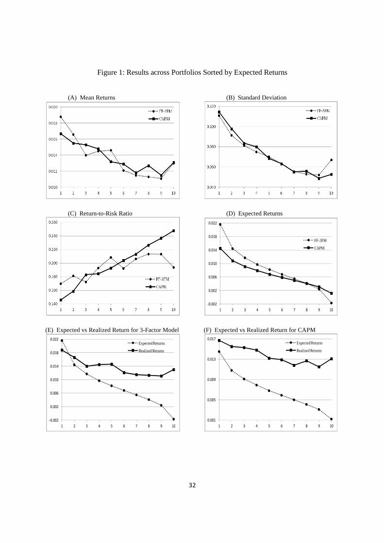
We summarize our findings with graphical presentation shown in Figure 1.
Panels A and B of figure 1 illustrate the comparative ability of the two models to create
consistent risk-return tradeoffs based on expected returns. As shown in Panel A, both models

18
produce portfolios where actual returns across portfolios vary with perceived risk. For both
models Portfolio 10, which should have both the lowest risk and return, has a higher return than
some of the other portfolios. For the FF-3FM returns to Portfolio 1 and 2 seem especially large
relative to the other portfolios suggesting that an investor seeking high returns may benefit from
information provided by the FF-3FM.
Panel B shows the realized risk for the FF-3FM and the CAPM. Both models show an
expected variation with realized risk falling with expected risk across portfolios one through ten.
Indeed, the risk level variation for the portfolios formed from both models is very similar. That
is, Portfolio 1 of the FF-3FM produces risk levels very similar to the risk level produced by
Portfolio 1 formed using the CAPM. For both models Portfolio 10 displays higher risk than
expected consistent with the higher than expected return. This is exception is especially
pronounced for the FF-3FM, suggesting a low reward-to-risk ratio for this portfolio.
Panel C shows the reward-to-risk ratios for both sets of portfolios. Both models show a
steady increase in the reward-to-risk ratio as expected portfolio risk/return increases. This effect
is especially pronounced for the CAPM. High return CAPM investors get a smaller payment for
risk than FF-3FM investors, but low risk investors using the CAPM model receive a higher
payment for risk. An investor may use the FF-3FM to achieve an expected risk-return tradeoff,
but the results do not appear to be clearly superior to what can be achieved from the CAPM.
Other considerations seem to favor the CAPM. Panel D shows expected returns across
portfolios for the FF-3FM and the CAPM. The FF-3FM has stronger outliers for Portfolio 1 and
Portfolio 10. This may be seen as a benefit for the high risk investor, but for the low risk
investor the prospect of a negative return cannot be appetizing. Panels E and F compare the

19
realized return with expected returns for the portfolios formed by the two models. 5 For the FF-
3FM the outliers for the extreme portfolios are moderated and the range of portfolio returns
becomes closer for the two models. The range of the expected excess returns for the 10
portfolios formed from the FF-3FM is 2.33% compared to 1.33% for the CAPM portfolios. The
range for the actual returns across portfolios is 0.58% for the FF-3FM compared to 0.36% for the
CAPM. This moderation would be especially comforting for the low-risk investor selecting to
use the FF-3FM, but these results suggest that the FF-3FM may produce inefficiencies in terms
of risk-adjustment procedures resulting from inconsistencies between realized and estimated
betas.
To the extent that the CAPM produces results that confirm to the results produced by the
FF-3FM, the question arises as to whether the results of the FF-3FM are dependent on the
CAPM’s MKT beta. We also seek to identify the inconsistencies in the FF-3FM betas that
created differences in expected and actual returns especially for the extreme portfolios. Further,
we seek to explore the cause of the superior performance of the high-risk FF-3FM portfolio
relative to the high-risk CAPM portfolio and the more consistent reward-to-risk portfolios of the
FF-3FM. In the next section we dissect the performance of both models, beginning with creating
returns for a two-factor Fama-French model.
III. Dissecting Model Performance: FF-3FM and CAPM
In Section II we reported performance results for portfolios based on the FF-3FM and the
CAPM. We find that both of these models are efficient in creating portfolios that vary along a
5 Notice for both portfolios the average actual returns are larger than average expected returns. This is consistent
with previous literature. For instance see Jegadeesh and Titman (1993) which studies momentum strategies
showing the superior performance of winners to losers. Both portfolios of these extreme portfolios and all other
portfolios show higher average returns than historic returns to market indexes.

20
risk-return continuum. Because both present certain deficiencies and because the CAPM MKT
beta is included in the FF-3FM, we repeat our portfolio formation procedure building portfolios
based solely on the HML beta and the SMB beta. We determine these betas values by applying
the FF-3FM equation during the estimation period. We estimate expected returns using the betas
from the SMB and HML factors as shown in equation (7) and use these expected returns to form
ten portfolios which should vary on a risk-return continuum:
������ = �� ∗ ������������ +�� ∗ ����������� (7)
where all variables are as defined earlier.
As above, we hold the portfolios for a one-year period and record average returns and the
standard deviation in returns. We seek to determine if the MKT beta is a necessary input to
achieve separation in risk and return across portfolios. Further, we seek to identify which of the
irregularities in results for the FF-3FM are dependent on the inclusion of the MKT beta and
whether other irregularities not found in the CAPM results are magnified with the exclusion of
the MKT beta.
Results for the two-factor HML-SMB beta model (2F-HSB model) are reported in Panel
A of Table 2. The results show that the MKT beta is not a necessary input to create portfolios
which will produce average returns whose ranks are consistent with rankings based on expected
returns. The 2F-HSB model produces correlation in expected and realized returns that is very
consistent with the results produced by the FF-3FM and the CAPM. All three models produce
similar Spearman rank order coefficients for expected and realized portfolio return. These range
between 0.8182 for the 2F-HSB model, 0.8303for the FF-3FM, and 0.8667 for the CAPM. In all

21
three cases the results are significant at the 0.5% level or lower. These results are certainly
inconsistent with the theoretical contention of the CAPM that MKT beta is the only factor
affecting expected returns for portfolios large enough to eliminate non-systematic risk. Just as
certainly, the results reported in Table 1 are inconsistent with the argument that the MKT beta
does not predict returns.
Both the FF-3FM and the CAPM produced portfolio segmentation whereby the portfolio
with the lowest expected return, Portfolio 10, had actual returns much higher than expected.
This result could be due to the impact of the MKT beta. Elimination of the MKT beta, however,
does not cause Portfolio 10 to have a low average return consistent with expectation. Portfolio
10 created with the 2F-HSB model has the fifth highest return of all portfolios.
Elimination of the MKT beta had a more significant result on portfolio risk. If betas from
the HML and SMB factors measure risk, portfolios formed with higher betas ought to produce
more variation in return. The Spearman’s correlation between expected risk and realized
standard deviation in 2F-HSB is much less than it is for the FF-3FM which includes the MKT
beta. More telling this correlation is much less than the predicted and realized risk for the
CAPM which only includes the MKT beta. The rank order correlation between expected and
realized risk for the 2F-HSB model is 0.5758 much lower than the rank order correlation of
0.9758 for the CAPM portfolios. The correlation coefficient for the 2F-HSB model is not
significant at the 5% level. To determine portfolio risk MKT beta seems to be required or either
the HML beta or SMB beta needs to be omitted. Of special note investors who seek to manage
risk should not consider the combined input from the HML betas or SML betas. Portfolio 10
formed by the 2F-HSB which should have the lowest risk based on expected return has the third
highest risk of all ten portfolios and the lowest reward-to-risk for all ten portfolios.

22
Ignoring the MKT beta of a security in portfolio formation does eliminate the significant
inverse trend in the reward-to-risk ratio across portfolios found for the CAPM and the FF-3FM
portfolios. If the MKT beta is not considered in portfolio the Spearman rank correlation between
expected risk and reward for risk turns from significantly negative to positive but insignificant.
High MKT beta securities seem in some sense to be inadequately compensated for risk.
Elimination of consideration of the MKT beta results in a portfolio formation process that
still efficiently predicts relative return but does not predict relative risk. This result suggests
caution in applying the FF-3FM to risk adjustment procedures. This caution is magnified by
examination of the expected excess returns provided by the 2F-HSB model. Without
consideration of the MKT beta the expected excess returns for the three lowest risk portfolios is
negative. Of course, this is an absurd result and argues for consideration of the CAPM’s MKT
beta in determining expected return and in risk adjustment in empirical studies. For portfolios 8,
9 and 10, a positive risk-adjusted return can be achieved with a negative return. This means that
based on estimations using only SMB and MKT betas approximately 30% of the securities in the
sample have negative expected excess returns. For these securities if risk-adjustment procedures
are conducted using measures of systematic risk determined in a sample period, test period
positive risk-adjusted returns may result with negative realized returns. It would presumably be
of little satisfaction for an investor to learn that the portfolio which is being held has a positive
risk-adjusted return when the realized return is negative. This type of perverse result occurs if
the SMB and HML betas are considered in risk-adjustment and becomes a significant result if
the CAPM MKT beta is not included. This result argues against the use of the HML and SMB
betas and by inference the FF-3FM in risk-adjustment procedures.

23
We have examined the efficiency of the MKT beta alone in creating portfolios with an
efficient risk-return tradeoff, but we have had not considered the efficiency of the HML and the
SMB betas in this regard. Because of the mixed results of using the 2F-HSB model we feel
obliged to investigate the result from using them singularly as further decomposition of the FF-
3FM and as further comparison to the CAPM. We estimate betas using equations (8) and (9) as
shown below:
������ = �� ∗ ������������ (8)
������ = �� ∗ ����������� (9)
where all variables are as defined earlier. We use identical portfolio formation and testing
procedures.
Panel B shows the results of building risk-return portfolios based on security’s loadings
on the HML factor. The results present strong contrasts to results presented under previous
specifications. Building portfolios based on the HML beta creates portfolios whose ranked
realized returns vary in order with rank expected return. Just as the CAPM one-factor model will
create portfolios whose realized returns are ordered consistent with expectations, a one-factor
model based on the HML beta will do likewise. Indeed, the ordering using the single factor
loading on the HML factor is more efficient than the ordering created by the FF-3FM, the CAPM
or the 2F-HSB model. The Spearman rank order coefficient between expected and realized
returns for the one-factor HML model is 0.9152. Of special note, Portfolio 10 which has realized
returns of between 1.30% and 1.38% in the previous three models has realized returns of 1.14%
24
for the HML one-factor model. The HML beta seems more efficient than any other factor
loading in identifying securities that will have high or low realized returns.
Portfolio managers may be able to rely on the HML beta to form portfolios whose returns
vary directly with factor loading, but the HML beta does not by itself provide a reasonable
prediction of the level of return. HML Portfolios 6 through 10 have negative expected excess
returns. That is according to a single factor HML model, approximately 50% of the securities in
the sample are expected to have negative excess returns. Because the value for the HML factor
is on average positive, these negative expected values indicate negative factor loadings on the
HML factor for approximately half of the securities. The results are troubling on several levels.
If responsiveness to changes in the HML is a measure of systematic risk, what sense does it
make for approximately half of the securities to have negative risk premiums based on exposure
to this systematic risk? How can a negative factor loading be stable if it implies a negative
expected return? If the betas are not stable, how can these factor loadings be used to adjust for
risk based on the systematic risk of a portfolio. Finally, if the negative betas are stable then the
portfolios formed on the basis of this systematic risk factor cannot possibly associate with
realized risk. Consider the following: Assume that the portfolios with the positive betas and the
portfolios with negative betas have the same absolute values along a continuum from high to low
absolute values. Thus, Portfolio 10 and Portfolio 1 will have the same absolute value for the
HML beta, but for Portfolio 10 the value is negative and for Portfolio 1 the value is positive.
The same would occur for Portfolio 9 and Portfolio 2 and so on with Portfolios 6 and 5 having
the same absolute value with different signs. In this case what would we expect in terms of
standard deviation if betas in the sample period and the estimation period are consistent?
Portfolios 10 and 1 with the largest absolute values in HML betas should have the highest
25
variation in return although Portfolio 10’s return would be positive when Portfolio’s 1 is negative
and vice versa. The standard deviation in returns would reduce across portfolios pairs with
Portfolios 5 and 6 having the lowest variation in realized return. Risk-adjusting returns based on
a systematic risk factor for which a significant portion of the securities have a negative loading
does not seem logical. We examine this dilemma further by first examining the stability of the
HML betas and then by examining the realized variation in returns for the HML portfolios.
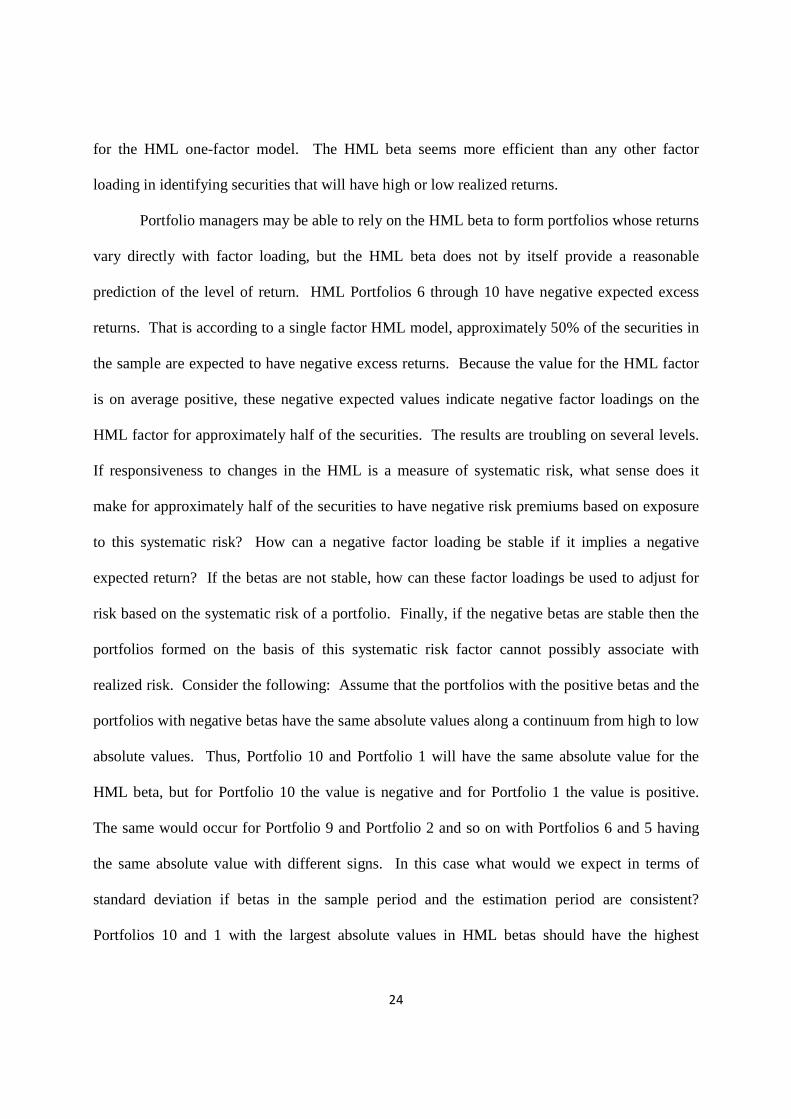
Figure 2 shows a comparison between realized and expected HML betas. The expected
beta reported in Figure 2 is derived by averaging the expected beta for each portfolio from
Portfolio 1 through Portfolio 10 across the eighty sample periods. The expected HML betas for
each sample period are simply the average of the betas for the individual securities that comprise
each portfolio in a particular sample period. The realized beta is determined by employing
equation (8) once again, but this time regressing realized return for each portfolio in each test
period against the HML factor. Thus, this regression holds 960 observations, twelve monthly
observations in each of the eighty one-year test periods.
The results reported in Figure 2 are consistent with both realized and expected returns
reported in Panel (B) of Table 2. Negative expected excess returns for Portfolios 6 through 10
are consistent with negative expected betas for Portfolios 6 through 10. The positive realized
returns reported in Table 2 for all HML portfolios are consistent with positive realized betas
across all portfolios for the HML betas except for Portfolio 10 where the coefficient is slightly
negative. These results may prove comforting for portfolio managers who would like to use the
HML beta to build low-risk, but positive return portfolios, but the results again strongly argue
against the use of historic HML betas in risk-adjusting portfolio returns. Negative factor
loadings which when applied in risk adjustment procedures suggest that a portfolio manager

26
could “beat the market” with returns less than the risk-free rate seem fundamentally
inappropriate.
The relationship with expected risk as measured by the systematic risk factor from
loading on the HML factor also fails to efficiently predict realized risk for the HML portfolios.
Although the sample Spearman rank correlation coefficient between expected risk and realized
risk is positive, it is not statistically significant different from zero. Portfolio 10 which should
have the lowest realized risk has the third highest realized risk. The Portfolios with high
expected returns, achieve these returns without significantly higher levels of risk. Thus, the
significantly negative correlation between the reward-to-risk ratio and expected return produced
by both the CAPM and the FF-3FM is replaced by a marginally significant positive correlation
between expected return and the reward-to-risk ratio.
To continue our decomposition of the FF-3FM we examine the performance of the SMB
beta in forming portfolios along a risk-return continuum. Results reported in Panel C of Table 2
show the performance of portfolios formed on the SMB beta found using equation (9). Test and
estimation procedures are identical to those used above. These results show that any one of the
three factor loadings used in the FF-3FM by itself can efficiently identify securities to be placed
in a return continuum. The SMB beta is more efficient in identifying high and low return
securities than either the HML beta, MKT beta or the FF-3FM as it produces the highest rank
correlation between actual and expected return. Unlike the HML beta, the SMB beta efficiently
predicts realized risk variation based on factor risk loadings. Although the SMB beta is not as
efficient as the CAPM in predicting realized risk. In particular Portfolio 10 shows much higher
variation in return than expected based on its factor loading. The use of the SMB beta alone
greatly reduces the creation of portfolios with expected negative returns that were found by the

27
use of the HML beta alone. Only Portfolio 10 has a negative expected return. Similar to the
results for the HML beta, actual returns for Portfolio 10 are positive and higher than other
portfolios with low expected risk. Again the CAPM outperforms both the single-factor SMB
model in this regard. Also, similar to the results with the CAPM, the single factor SMB model
produces a significant inverse relationship between expected return and the risk-return tradeoff,
although this relationship is weaker than that found for the CAPM. Because, both the CAPM
and the single factor SMB model outperform the single factor HML model in terms of predicting
risk, we combine the SMB beta and the MKT beta into a two-factor model and compare results
from this model to the results of previous models.
As we did with the 2F-HSB model we use the beta estimates derived from Equation (6) to
form the two-factor MKT-SMB (2F-MSB). The same sampling and test procedures are used as
with the other models. The results are reported in Table 3.
The results for the two-factor SMB-MKT beta model compare favorably with the results
for the FF-3FM. The 2F-MSB model produces more efficient separation in terms of both
realized return and risk than does the FF-3FM. The 2F-MSB model is more efficient than the
CAPM in predicting realized return and as efficient as the CAPM in predicting realized risk.
The inclusion of the MKT beta with the SMB beta reduces the risk of Portfolio 10 and eliminates
the negative expected return of Portfolio 10 when the latter beta is used alone. The inclusion of
the MKT beta, however, increases the tendency for the reward-to-risk ratio to fall as expected
return increases. In some sense securities with high MKT betas appear to be inadequately
compensated for risk. Because the FF-3FM is an empirical rather than a theoretical model, one
is hard pressed to argue for its superiority to the 2F-MSB model.

28
IV. Conclusion
We identify two regimes in the measurement of systematic risk during the era of modern
portfolio theory. The Capital Asset Pricing Model, CAPM, a theoretical based model, was
replaced by the empirical, Fama-French three-factor model, FF-3FM, in part based on the finding
by Fama and French (1992) that a positive relationship does not exist between a security’s
covariance with the market and the security’s return. This same study confirmed previous
findings of a positive relationship between security’s book-to-market value and return, and a
security’s market value and return. Together these findings led to the creation of the FF-3FM.
Although the FF-3FM is widely used to measure systematic risk in academic studies, it has not
been subjected to out-of-sample testing to validate the model’s ability to measure systematic risk
and predict return and its variation.
In part the failure to study the relationship between systematic risk as measured by the
FF-3FM and returns results from the model’s failure to have a single measure for risk as does the
CAPM. We study the relationship between systematic risk and return by building portfolios
based on expected risk as measured by the FF-3FM and compare the realized return and risk of
these portfolios. We find that the FF-3FM does accurately predict variation along a risk-return
continuum. Ironically, when we include the CAPM using the same procedures for comparisons
purpose we find that the CAPM is roughly as efficient as the FF-3FM in creating portfolios that
vary along a risk return continuum. Moreover, we find certain deficiencies in the FF-3FM, low-
risk portfolios are predicted to have negative excess returns and high risk portfolios have
outsized expected returns. We find that these deficiencies largely result from inclusion of the
loading on the zero-investment portfolio associated with the book to market ratio. We find that a
two-factor model including the market beta and the size related beta appears to be a more

29
efficient predictor of returns and risk than the FF-3FM. Because the FF-3FM is not theoretically
based, it appears to be an open question as to why this model should be used to predict risk and
return. Further research should be conducted to provide answers to this question.

30
References
Banz, R. (1981). The relationship between return and market value of common stocks. Journal of Financial Economics 9, 3–18. Bartholdy, Jan and Paula Peare. (2005). Estimation of expected return: CAPM vs. Fama and French. International Review of Financial Analysis: 14 (4), p. 407. Black, F., M. Jensen, and M. Scholes (1972). The capital asset pricing model: Some empirical tests. Studies in the Theory of Capital Markets. Praeger, New York, 79–121. Estrada, Javier. (2011). The Three‐Factor Model: A Practitioner's Guide. The Bank of America Journal of Applied Corporate Finance: 23 (2), p. 77-85. Fama, E. and K. French (1992). The cross-section of expected stock returns. Journal of Finance 47, 427–465. Fama, E. and K. French (1993). Common risk factors in the returns on stocks and bonds. Journal of Financial Economics 33, 3–56. Fama, E. and J. MacBeth (1973). Risk, return, and equilibrium: Empirical tests. Journal of Political Economy 81, 607–636. Fletcher, J. (1997). An examination of the cross-sectional relationship of beta and returns: UK evidence. Journal of Business and Economics 49, 211-21. Graham, John and Campbell Harvey. (2001). The theory and practice of corporate finance: Evidence from the field. Journal of Financial Economics: 60 (2-3), pp. 187-243. Jegadeesh, N. & Titman, S. (1993). Returns to Buying Winners and Selling Losers: Implications for Stock Market Efficiency. Journal of Finance, 48, 65-91. Koch S. and C. Westheide (2010). The conditional relation between Fama-French betas and return. Working paper, University of Bonn. Lintner, J. (1965). The valuation of risk assets and the selection of risky investments in stock portfolios and capital budgets. Review of Economics and Statistics 47(13-37). Markowits, H. (1952). Portfolio selection. Journal of Finance 7, 77-91. Mossin, J. (1966). Equilibrium in a capital asset market. Econometrica 34, 768–783. Pettengill, G., S. Sundaram, and I. Mathur (2002). Payment for risk: constant beta vs. dual-beta models. Financial Review 37, 123–136. Pettengill, G., S. Sundaram, and I. Mathur (1995). The conditional relation between

31
beta and return. Journal of Financial and Quantitative Analysis 30, 101–116. Reinganum, M. (1981). A new empirical perspective on the CAPM. Journal of Financial and Quantitative Analysis 16, 439–462. Rosenberg, B, K. Reid, and R. Lanstein (1985). Pervasive evidence of market inefficiency Journal of Portfolio Management, 11, 9-17. Sharpe, W. (1964). Capital asset prices: A theory of market equilibrium under conditions of risk. Journal of Finance 19, 425–442. Tinic S. and R. West (1984). Risk and return: January vs. the rest of the year. Journal of Financial Economics 13, 107-124.
32
Figure 1: Results across Portfolios Sorted by Expected Returns (A) Mean Returns (B) Standard Deviation
(C) Return-to-Risk Ratio (D) Expected Returns
(E) Expected vs Realized Return for 3-Factor Model (F) Expected vs Realized Return for CAPM
-0.002
0.002
0.006
0.010
0.014
0.018
0.022
1 2 3 4 5 6 7 8 9 10
FF-3FM
CAPM
-0.002
0.002
0.006
0.010
0.014
0.018
0.022
1 2 3 4 5 6 7 8 9 10
Expected Returns
Realized Returns
0.001
0.005
0.009
0.013
0.017
1 2 3 4 5 6 7 8 9 10
Expected Returns
Realized Returns

33
-2
-1.5
-1
-0.5
0
0.5
1
1.5
2
2.5
1 2 3 4 5 6 7 8 9 10
Be
ta V
alu
e
Portfolio
Estimated Betas
Realized Betas
Figure 2: Estimated Beta vs. Realized Beta for HML Factor

34
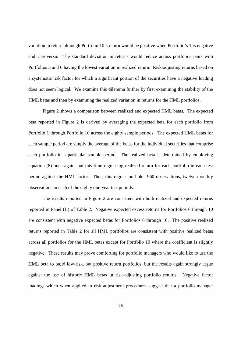
Table 1: Portfolios sorted by expected returns Portfolios sorted by expected returns from the highest (1) to the lowest (10) Spearman's Rank 1 2 3 4 5 6 7 8 9 10 Rho P-value
(A) FF-3FMa Expected return 0.0216 0.0144 0.0117 0.0097 0.0082 0.0068 0.0055 0.0041 0.0024 -0.0017 --- ---
Realized returns 0.0188 0.0166 0.0140 0.0145 0.0146 0.0121 0.0115 0.0113 0.0111 0.0130 0.8303 0.0022
Std Dev of return 0.1111 0.0914 0.0814 0.0749 0.0702 0.0631 0.0556 0.0529 0.0521 0.0671 0.8788 0.0004
Return/Risk ratio 0.1696 0.1812 0.1723 0.1929 0.2084 0.1923 0.2061 0.2134 0.2133 0.1937 -0.7818 0.0070 (B) CAPMb
Expected return 0.0145 0.0108 0.0091 0.0079 0.0068 0.0059 0.0050 0.0041 0.0031 0.0012 --- --- Realized returns 0.0167 0.0155 0.0153 0.0148 0.0132 0.0129 0.0118 0.0127 0.0115 0.0131 0.8667 0.0007
Std Dev of return 0.1147 0.0979 0.0836 0.0801 0.0686 0.0633 0.0552 0.0560 0.0488 0.0528 0.9758 0c
Return/Risk ratio 0.1456 0.1586 0.1830 0.1843 0.1927 0.2040 0.2131 0.2265 0.2367 0.2479 -1.0000 0
a. FF-3FM: Fama-French three-factor model. Stocks are sorted by the estimated returns from the following equation: , where are the estimated betas from the regression
during the three-year estimation periods, and is the mean of the X factor (X=MKT,
SMB, or HML) from the entire sample period (1927-2009). The reported realized return is the mean of the monthly portfolio returns from the 80 holding periods after the estimation periods.
b. CAPM: Stocks are sorted by the estimated returns from the following equation: , where is the estimated
beta from the regression during the three-year estimation periods. The reported realized return is the mean of
the monthly portfolio returns from the 80 holding periods after the estimation periods. c. These P-Values are nonzero but small than 0.00005.
ˆ ˆ ˆˆ ( )it im is ihE R MKT SMB HMLβ β β= ⋅ + ⋅ + ⋅ ˆ 'i sβ
it im t is t ih t itR MKT SMB HMLβ β β ε= ⋅ + ⋅ + ⋅ + X
ˆˆ ( )it imE R MKTβ= ⋅ ˆimβ
it im t itR MKTβ ε= ⋅ +

35
Table 2: Portfolios sorted by expected returns Portfolios sorted by expected returns from the highest (1) to the lowest (10) Spearman's Rank 1 2 3 4 5 6 7 8 9 10 Rho P-value
(A) Two-Factor Model (2F-HSB)a Expected return 0.0128 0.0069 0.0047 0.0033 0.0021 0.0011 0.0002 -0.0009 -0.0025 -0.0062 --- ---
Realized returns 0.0196 0.0155 0.0148 0.0145 0.0134 0.0125 0.0112 0.0111 0.0111 0.0138 0.8182 0.0031
Std Dev of return 0.1073 0.0873 0.0730 0.0723 0.0653 0.0575 0.0559 0.0573 0.0627 0.0816 0.5758 0.0918
Return/Risk ratio 0.1827 0.1769 0.2034 0.2005 0.2057 0.2181 0.2007 0.1935 0.1763 0.1697 0.2727 0.4721 (B) Single-Factor Model - HMLb
Expected return 0.0091 0.0050 0.0033 0.0020 0.0010 -2x10⁻⁶ -0.0010 -0.0022 -0.0038 -0.0076 --- --- Realized returns 0.0185 0.0172 0.0155 0.0149 0.0148 0.0123 0.0109 0.0113 0.0109 0.0114 0.9152 0.0001
Std Dev of return 0.0971 0.0935 0.0764 0.0713 0.0673 0.0640 0.0602 0.0620 0.0660 0.0800 0.5758 0.0918
Return/Risk ratio 0.1904 0.1840 0.2023 0.2082 0.2203 0.1917 0.1819 0.1816 0.1653 0.1421 0.6606 0.0413
(C) Single-Factor Model - SMBc
Expected return 0.0065 0.0042 0.0032 0.0026 0.0021 0.0016 0.0012 0.0008 0.0002 -0.0007 --- ---
Realized returns 0.0171 0.0168 0.0154 0.0148 0.0133 0.0130 0.0121 0.0118 0.0110 0.0123 0.9273 0d
Std Dev of return 0.1115 0.0959 0.0845 0.0732 0.0675 0.0621 0.0561 0.0543 0.0509 0.0645 0.8788 0.0004
Return/Risk ratio 0.1535 0.1748 0.1824 0.2017 0.1973 0.2095 0.2164 0.2171 0.2151 0.1907 -0.6970 0.0269
a. 2F-HSB: Stocks are sorted by the estimated returns from the following equation: ˆ ˆˆ ( ) ,it is ihE R SMB HMLβ β= ⋅ + ⋅ where are
the estimated betas from the regression during the three-year estimation periods, and
is the mean of the X factor (X= SMB or HML) from the entire sample period (1927-2009). The reported realized return is the mean of the monthly portfolio returns from the 80 holding periods after the estimation periods.
b. Single-Factor Model - HML: Stocks are sorted by the estimated returns from the following equation: ˆˆ( ) ,it ihE R HMLβ= ⋅ where
ihβ is the estimated beta from the regression it ih t itR HMLβ ε= ⋅ + during the three-year estimation periods. The reported realized
return is the mean of the monthly portfolio returns from the 80 holding periods after the estimation periods.
c. Single-Factor Model - SMB: Stocks are sorted by the estimated returns from the following equation: ˆˆ( ) ,it isE R SMBβ= ⋅ where isβ
is the estimated beta from the regression it is t itR SMBβ ε= ⋅ + during the three-year estimation periods. The reported realized return
is the mean of the monthly portfolio returns from the 80 holding periods after the estimation periods. d. These P-Values are nonzero but small than 0.00005.
ˆ 'i sβit im t is t ih t itR MKT SMB HMLβ β β ε= ⋅ + ⋅ + ⋅ +
X

36
Table 3: Portfolios sorted by expected returns using MKT and SMB factors (2F-MSB model) Portfolios sorted by expected returns from the highest (1) to the lowest (10) Spearman's Rank 1 2 3 4 5 6 7 8 9 10 Rho P-value
Expected return 0.0158 0.0114 0.0097 0.0084 0.0074 0.0064 0.0055 0.0046 0.0035 0.0013 --- ---
Realized returns 0.0173 0.0159 0.0141 0.0145 0.0135 0.0138 0.0115 0.0122 0.0115 0.0130 0.8909 0.0002
Std Dev of return 0.1089 0.0958 0.0822 0.0756 0.0693 0.0642 0.0569 0.0583 0.0505 0.0539 0.9758 0*
Return/Risk ratio 0.1593 0.1655 0.1720 0.1918 0.1949 0.2146 0.2029 0.2094 0.2276 0.2420 -0.9636 0*
Stocks are sorted by the estimated returns from the following equation: ˆ ˆˆ( ) ,it im isE R MKT SMBβ β= ⋅ + ⋅ where are the estimated
betas from the regression during the three-year estimation periods, and is the mean of
the X factor (X= SMB or HML) from the entire sample period (1927-2009). The reported realized return is the mean of the monthly portfolio returns from the 80 holding periods after the estimation periods. * These P-Values are nonzero but small than 0.00005.
ˆ 'i sβ
it im t is t ih t itR MKT SMB HMLβ β β ε= ⋅ + ⋅ + ⋅ + X