RISK Portfolio Theory and the Capital Asset Pricing Model

● ● ● ● ●

confirming pages

185

PART 2

◗ In Chapter 7 we began to come to grips with the problem of measuring risk. Here is the story so far.

The stock market is risky because there is a spread of possible outcomes. The usual measure of this spread is the standard deviation or variance. The risk of any stock can be broken down into two parts. There is the specific or diversifiable risk that is peculiar to that stock, and there is the market risk that is associated with marketwide variations. Investors can eliminate specific risk by holding a well-diversified portfolio, but they cannot eliminate market risk. All the risk of a fully diversified portfolio is market risk.

A stock’s contribution to the risk of a fully diversified portfolio depends on its sensitivity to market changes. This sensitivity is generally known as beta. A security with a beta of 1.0 has average market risk—a well-diversified portfolio of such securities has the same

standard deviation as the market index. A security with a beta of .5 has below-average market risk—a well-diversified portfolio of these securities tends to move half as far as the market moves and has half the market’s standard deviation.

In this chapter we build on this newfound knowledge. We present leading theories linking risk and return in a competitive economy, and we show how these theories can be used to estimate the returns required by investors in different stock-market investments. We start with the most widely used theory, the capital asset pricing model, which builds directly on the ideas developed in the last chapter. We will also look at another class of models, known as arbitrage pricing or factor models. Then in Chapter 9 we show how these ideas can help the financial manager cope with risk in practical capital budgeting situations.

Portfolio Theory and the Capital Asset Pricing Model

8 CHAPTER

RISK

Most of the ideas in Chapter 7 date back to an article written in 1952 by Harry Markowitz.1 Markowitz drew attention to the common practice of portfolio diversification and showed exactly how an investor can reduce the standard deviation of portfolio returns by choos-ing stocks that do not move exactly together. But Markowitz did not stop there; he went on to work out the basic principles of portfolio construction. These principles are the foundation for much of what has been written about the relationship between risk and return.

We begin with Figure 8.1, which shows a histogram of the daily returns on IBM stock from 1988 to 2008. On this histogram we have superimposed a bell-shaped normal

1 H. M. Markowitz, “Portfolio Selection,” Journal of Finance 7 (March 1952), pp. 77–91.

8-1 Harry Markowitz and the Birth of Portfolio Theory

● ● ● ● ●

bre30735_ch08_185-212.indd 185bre30735_ch08_185-212.indd 185 12/2/09 7:28:28 PM12/2/09 7:28:28 PM

confirming pages

186 Part Two Risk

d istribution. The result is typical: When measured over a short interval, the past rates of return on any stock conform fairly closely to a normal distribution.2

Normal distributions can be completely defined by two numbers. One is the average or expected return; the other is the variance or standard deviation. Now you can see why in Chapter 7 we discussed the calculation of expected return and standard deviation. They are not just arbitrary measures: if returns are normally distributed, expected return and stan-dard deviation are the only two measures that an investor need consider.

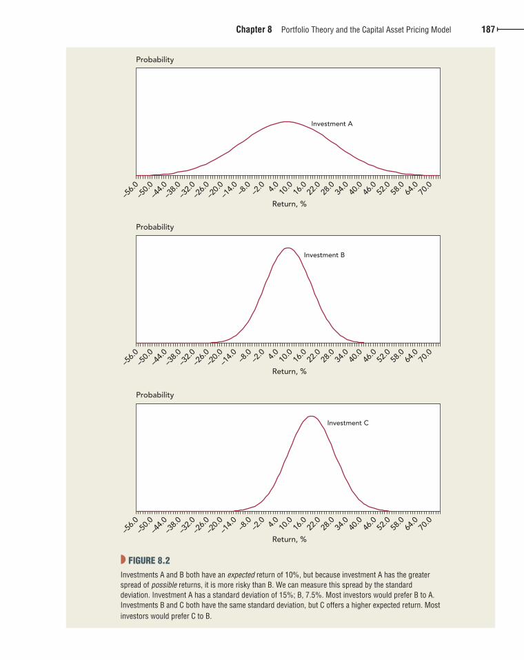
Figure 8.2 pictures the distribution of possible returns from three investments. A and B offer an expected return of 10%, but A has the much wider spread of possible outcomes. Its standard deviation is 15%; the standard deviation of B is 7.5%. Most investors dislike uncertainty and would therefore prefer B to A.

Now compare investments B and C. This time both have the same standard deviation, but the expected return is 20% from stock C and only 10% from stock B. Most investors like high expected return and would therefore prefer C to B.

Combining Stocks into PortfoliosSuppose that you are wondering whether to invest in the shares of Campbell Soup or Boeing. You decide that Campbell offers an expected return of 3.1% and Boeing offers an expected return of 9.5%. After looking back at the past variability of the two stocks, you also decide that the standard deviation of returns is 15.8% for Campbell Soup and 23.7% for Boeing. Boeing offers the higher expected return, but it is more risky.

Now there is no reason to restrict yourself to holding only one stock. For example, in Section 7-3 we analyzed what would happen if you invested 60% of your money in Camp-bell Soup and 40% in Boeing. The expected return on this portfolio is about 5.7%, simply a weighted average of the expected returns on the two holdings. What about the risk of such a portfolio? We know that thanks to diversification the portfolio risk is less than the a verage

2 If you were to measure returns over long intervals, the distribution would be skewed. For example, you would encounter returns greater than 100% but none less than � 100%. The distribution of returns over periods of, say, one year would be better approxi-mated by a lognormal distribution. The lognormal distribution, like the normal, is completely specified by its mean and standard deviation.

◗ FIGURE 8.1 Daily price changes for IBM are approximately normally distributed. This plot spans 1988 to 2008.

–5.6–7 –2.8–4.2 –1.4 0 1.4 4.22.8 5.6 7 7.70

0.5

1

1.5

2

2.5

3

3.5

4

% o

f d

ays

Daily price changes, %


confirming pages

Chapter 8 Portfolio Theory and the Capital Asset Pricing Model 187

–56.0

–50.0

Return, %

Probability

Probability

Probability

Investment A

–44.0

–38.0

–32.0

–26.0

–20.0

–14.0 –8

.0–2

.0 4.0 10.0

16.0

22.0

28.0

34.0

40.0

46.0

52.0

58.0

64.0

70.0

–56.0

–50.0

Return, %

Investment B

–44.0

–38.0

–32.0

–26.0

–20.0

–14.0 –8

.0–2

.0 4.0 10.0

16.0

22.0

28.0

34.0

40.0

46.0

52.0

58.0

64.0

70.0

–56.0

–50.0

Return, %

Investment C

–44.0

–38.0

–32.0

–26.0

–20.0

–14.0 –8

.0–2

.0 4.0 10.0

16.0

22.0

28.0

34.0

40.0

46.0

52.0

58.0

64.0

70.0

◗ FIGURE 8.2 Investments A and B both have an expected return of 10%, but because investment A has the greater spread of possible returns, it is more risky than B. We can measure this spread by the standard d eviation. Investment A has a standard deviation of 15%; B, 7.5%. Most investors would prefer B to A. Investments B and C both have the same standard deviation, but C offers a higher expected return. Most investors would prefer C to B.


confirming pages

188 Part Two Risk

of the risks of the separate stocks. In fact, on the basis of past experience the standard devia-tion of this portfolio is 14.6%.3

The curved blue line in Figure 8.3 shows the expected return and risk that you could achieve by different combinations of the two stocks. Which of these combinations is best depends on your stomach. If you want to stake all on getting rich quickly, you should put all your money in Boeing. If you want a more peaceful life, you should invest most of your money in Campbell Soup, but you should keep at least a small investment in Boeing.4

We saw in Chapter 7 that the gain from diversification depends on how highly the stocks are correlated. Fortunately, on past experience there is only a small positive correla-tion between the returns of Campbell Soup and Boeing (� � �.18). If their stocks moved in exact lockstep (� � �1), there would be no gains at all from diversification. You can see this by the brown dotted line in Figure 8.3. The red dotted line in the figure shows a second extreme (and equally unrealistic) case in which the returns on the two stocks are perfectly negatively correlated (� � �1). If this were so, your portfolio would have no risk.

In practice, you are not limited to investing in just two stocks. For example, you could decide to choose a portfolio from the 10 stocks listed in the first column of Table 8.1. After analyzing the prospects for each firm, you come up with forecasts of their returns. You are most optimistic about the outlook for Amazon, and forecast that it will provide a return of 22.8%. At the other extreme, you are cautious about the prospects for Johnson & Johnson and predict a return of 3.8%. You use data for the past five years to estimate the risk of each stock and the correlation between the returns on each pair of stocks.5

Now look at Figure 8.4. Each diamond marks the combination of risk and return offered by a different individual security. For example, Amazon has both the highest standard deviation and the highest expected return. It is represented by the upper-right diamond in the figure.

3 We pointed out in Section 7-3 that the correlation between the returns of Campbell Soup and Boeing has been about .18. The variance of a portfolio which is invested 60% in Campbell and 40% in Boeing is

Variance 5 x12s1

2 1 x22s2

2 1 2x1x2� 12s1s2

5 3 1 .6 22 3 115.8 22 4 1 3 1 .4 22 3 123.7 22 4 1 2 1 .6 3 .4 3 .18 3 15.8 3 23.7 2

5 212.1

The portfolio standard deviation is "212.1 5 14.6%. 4 The portfolio with the minimum risk has 73.1% in Campbell Soup. We assume in Figure 8.3 that you may not take negative positions in either stock, i.e., we rule out short sales.

5 There are 45 different correlation coefficients, so we have not listed them in Table 8.1 .

Boeing

Campbell soup

40% in Boeing

0

1

2

3

4

5

6

7

8

9

10

252015100 5

Exp

ecte

d r

etur

n (r

), %

Standard deviation (σ), %

◗ FIGURE 8.3 The curved line illustrates how expected return and standard deviation change as you hold different combinations of two stocks. For example, if you invest 40% of your money in Boeing and the remain-der in Campbell Soup, your expected return is 12%, which is 40% of the way between the expected returns on the two stocks. The standard deviation is 14.6%, which is less than 40% of the way between the standard deviations of the two stocks. This is because diversifica-tion reduces risk.


confirming pages


◗ TABLE 8.1 Examples of efficient portfolios chosen from 10 stocks.

Note: Standard deviations and the correlations between stock returns were estimated from monthly returns, January 2004– December 2008. Efficient portfolios are calculated assuming that short sales are prohibited.

Efficient Portfolios—Percentages Allocated to Each Stock

StockExpected Return

Standard Deviation A B C

Amazon 22.8% 50.9% 100 10.9

Ford 19.0 47.2 11.0

Dell 13.4 30.9 10.3

Starbucks 9.0 30.3 10.7 3.6

Boeing 9.5 23.7 10.5

Disney 7.7 19.6 11.2

Newmont 7.0 36.1 9.9 10.2

Exxon Mobil 4.7 19.1 9.7 18.4

Johnson & Johnson 3.8 12.5 7.4 33.9

Campbell Soup 3.1 15.8 8.4 33.9

Expected portfolio return 22.8 10.5 4.2

Portfolio standard deviation 50.9 16.0 8.8

By holding different proportions of the 10 securities, you can obtain an even wider selection of risk and return: in fact, anywhere in the shaded area in Figure 8.4. But where in the shaded area is best? Well, what is your goal? Which direction do you want to go? The answer should be obvious: you want to go up (to increase expected return) and to the left (to reduce risk). Go as far as you can, and you will end up with one of the portfolios that lies along the heavy solid line. Markowitz called them efficient portfolios. They offer the highest expected return for any level of risk.

We will not calculate this set of efficient portfolios here, but you may be interested in how to do it. Think back to the capital rationing problem in Section 5-4. There we wanted to deploy a limited amount of capital investment in a mixture of projects to give the highest NPV. Here we want to deploy an investor’s funds to give the highest expected return for a given standard deviation. In principle, both problems can be solved by hunt-ing and pecking—but only in principle. To solve the capital rationing problem, we can employ linear programming; to solve the portfolio problem, we would turn to a variant of linear programming known as quadratic programming. Given the expected return and standard deviation for each stock, as well as the correlation between each pair of stocks, we could use a standard quadratic computer program to calculate the set of efficient portfolios.

Three of these efficient portfolios are marked in Figure 8.4. Their compositions are sum-marized in Table 8.1. Portfolio B offers the highest expected return: it is invested entirely in one stock, Amazon. Portfolio C offers the minimum risk; you can see from Table 8.1 that it has large holdings in Johnson & Johnson and Campbell Soup, which have the low-est standard deviations. However, the portfolio also has a sizable holding in Newmont even though it is individually very risky. The reason? On past evidence the fortunes of go ld-mining shares, such as Newmont, are almost uncorrelated with those of other stocks and so provide additional diversification.


confirming pages

190 Part Two Risk

Table 8.1 also shows the compositions of a third efficient portfolio with intermediate levels of risk and expected return.

Of course, large investment funds can choose from thousands of stocks and thereby achieve a wider choice of risk and return. This choice is represented in Figure 8.5 by the shaded, broken-egg-shaped area. The set of efficient portfolios is again marked by the heavy curved line.

We Introduce Borrowing and LendingNow we introduce yet another possibility. Suppose that you can also lend or borrow money at some risk-free rate of interest rf. If you invest some of your money in Treasury bills (i.e., lend money) and place the remainder in common stock portfolio S, you can obtain any combination of expected return and risk along the straight line joining rf and

A

0

5

10

15

20

25

20100 30 40 50 60Standard deviation (σ), %

C

B

Exp

ecte

d r

etur

n (r

), %

◗ FIGURE 8.4 Each diamond shows the expected return and standard deviation of 1 of the 10 stocks in Table 8.1 . The shaded area shows the possible combina-tions of expected return and standard deviation from invest-ing in a mixture of these stocks. If you like high expected returns and dislike high standard devia-tions, you will prefer portfolios along the heavy line. These are efficient portfolios. We have marked the three efficient port-folios described in Table 8.1 (A, B, and C).

rf

Expectedreturn (r),

%

S Borro

win

g

Lend

ing

T

Standard deviation (σ)

◗ FIGURE 8.5 Lending and borrowing extend the range of investment possibilities. If you invest in portfolio S and lend or borrow at the risk-free interest rate, r f , you can achieve any point along the straight line from r f through S. This gives you a higher expected return for any level of risk than if you just invest in common stocks.


confirming pages


S in Figure 8.5. Since borrowing is merely negative lending, you can extend the range of possibilities to the right of S by borrowing funds at an interest rate of rf and investing them as well as your own money in portfolio S.

Let us put some numbers on this. Suppose that portfolio S has an expected return of 15% and a standard deviation of 16%. Treasury bills offer an interest rate (rf ) of 5% and are risk-free (i.e., their standard deviation is zero). If you invest half your money in portfolio S and lend the remainder at 5%, the expected return on your investment is likewise halfway between the expected return on S and the interest rate on Treasury bills:

r 5 1 1@2 3 expected return on S 2 1 1 1@2 3 interest rate 2 5 10%

And the standard deviation is halfway between the standard deviation of S and the standard deviation of Treasury bills:6

s 5 1 1@2 3 standard deviation of S 2 1 1 1@2 3 standard deviation of bills 2 5 8%

Or suppose that you decide to go for the big time: You borrow at the Treasury bill rate an amount equal to your initial wealth, and you invest everything in portfolio S. You have twice your own money invested in S, but you have to pay interest on the loan. Therefore your expected return is

r 5 12 3 expected return on S 2 2 11 3 interest rate 2 5 25%

And the standard deviation of your investment is

s 5 12 3 standard deviation of S 2 2 11 3 standard deviation of bills 2 5 32%

You can see from Figure 8.5 that when you lend a portion of your money, you end up part-way between rf and S; if you can borrow money at the risk-free rate, you can extend your possibilities beyond S. You can also see that regardless of the level of risk you choose, you can get the highest expected return by a mixture of portfolio S and borrowing or lending. S is the best efficient portfolio. There is no reason ever to hold, say, portfolio T.

If you have a graph of efficient portfolios, as in Figure 8.5, finding this best efficient portfolio is easy. Start on the vertical axis at rf and draw the steepest line you can to the curved heavy line of efficient portfolios. That line will be tangent to the heavy line. The efficient portfolio at the tangency point is better than all the others. Notice that it offers the highest ratio of risk premium to standard deviation. This ratio of the risk premium to the standard deviation is called the Sharpe ratio:

Sharpe ratio 5Risk premium

Standard deviation5

r 2 rf

s

Investors track Sharpe ratios to measure the risk-adjusted performance of investment man-agers. (Take a look at the mini-case at the end of this chapter.)

We can now separate the investor’s job into two stages. First, the best portfolio of com-mon stocks must be selected—S in our example. Second, this portfolio must be blended with borrowing or lending to obtain an exposure to risk that suits the particular investor’s taste. Each investor, therefore, should put money into just two benchmark investments—a risky portfolio S and a risk-free loan (borrowing or lending).

6 If you want to check this, write down the formula for the standard deviation of a two-stock portfolio:

Standard deviation 5"x12s1

2 1 x22s2

2 1 2x1x2�12s1s2

Now see what happens when security 2 is riskless, i.e., when � 2 � 0.


confirming pages

192 Part Two Risk

What does portfolio S look like? If you have better information than your rivals, you will want the portfolio to include relatively large investments in the stocks you think are undervalued. But in a competitive market you are unlikely to have a monopoly of good ideas. In that case there is no reason to hold a different portfolio of common stocks from anybody else. In other words, you might just as well hold the market portfolio. That is why many professional investors invest in a market-index portfolio and why most others hold well-diversified portfolios.

In Chapter 7 we looked at the returns on selected investments. The least risky investment was U.S. Treasury bills. Since the return on Treasury bills is fixed, it is unaffected by what happens to the market. In other words, Treasury bills have a beta of 0. We also considered a much riskier investment, the market portfolio of common stocks. This has average market risk: its beta is 1.0.

Wise investors don’t take risks just for fun. They are playing with real money. There-fore, they require a higher return from the market portfolio than from Treasury bills. The difference between the return on the market and the interest rate is termed the market risk premium. Since 1900 the market risk premium (rm � rf ) has averaged 7.1% a year.

In Figure 8.6 we have plotted the risk and expected return from Treasury bills and the market portfolio. You can see that Treasury bills have a beta of 0 and a risk premium of 0.7 The market portfolio has a beta of 1 and a risk premium of rm � rf. This gives us two benchmarks for the expected risk premium. But what is the expected risk premium when beta is not 0 or 1?

In the mid-1960s three economists—William Sharpe, John Lintner, and Jack Treynor—produced an answer to this question.8 Their answer is known as the capital asset pricing

7 Remember that the risk premium is the difference between the investment’s expected return and the risk-free rate. For Treasury bills, the difference is zero. 8 W. F. Sharpe, “Capital Asset Prices: A Theory of Market Equilibrium under Conditions of Risk,” Journal of Finance 19 (September 1964), pp. 425–442; and J. Lintner, “The Valuation of Risk Assets and the Selection of Risky Investments in Stock Portfolios and Capital Budgets,” Review of Economics and Statistics 47 (February 1965), pp. 13–37. Treynor’s article has not been published.

8-2 The Relationship Between Risk and Return

◗ FIGURE 8.6 The capital asset pricing model states that the expected risk premium on each investment is proportional to its beta. This means that each investment should lie on the sloping security market line connecting Treasury bills and the market portfolio.

0 .5 1.0 2.0

Treasury bills

Market portfolio

Security market line

Expected returnon investment

rf

rm

beta


confirming pages


model, or CAPM. The model’s message is both startling and simple. In a competitive market, the expected risk premium varies in direct proportion to beta. This means that in Figure 8.6 all investments must plot along the sloping line, known as the security market line. The expected risk premium on an investment with a beta of .5 is, therefore, half the expected risk premium on the market; the expected risk premium on an invest-ment with a beta of 2 is twice the expected risk premium on the market. We can write this relationship as

Expected risk premium on stock 5 beta 3 expected risk premium on market r 2 rf 5 �1 rm 2 rf 2

Some Estimates of Expected ReturnsBefore we tell you where the formula comes from, let us use it to figure out what returns investors are looking for from particular stocks. To do this, we need three numbers: �, rf, and rm � rf. We gave you estimates of the betas of 10 stocks in Table 7.5. In February 2009 the interest rate on Treasury bills was about .2%.

How about the market risk premium? As we pointed out in the last chapter, we can’t measure rm � rf with precision. From past evidence it appears to be 7.1%, although many economists and financial managers would forecast a slightly lower figure. Let us use 7% in this example.

Table 8.2 puts these numbers together to give an estimate of the expected return on each stock. The stock with the highest beta in our sample is Amazon. Our estimate of the expected return from Amazon is 15.4%. The stock with the lowest beta is Campbell Soup. Our estimate of its expected return is 2.4%, 2.2% more than the interest rate on Treasury bills. Notice that these expected returns are not the same as the hypothetical forecasts of return that we assumed in Table 8.1 to generate the efficient frontier.

You can also use the capital asset pricing model to find the discount rate for a new capi-tal investment. For example, suppose that you are analyzing a proposal by Dell to expand its capacity. At what rate should you discount the forecasted cash flows? According to Table 8.2, investors are looking for a return of 10.2% from businesses with the risk of Dell. So the cost of capital for a further investment in the same business is 10.2%.9

9 Remember that instead of investing in plant and machinery, the firm could return the money to the shareholders. The opportu-nity cost of investing is the return that shareholders could expect to earn by buying financial assets. This expected return depends on the market risk of the assets.

◗ TABLE 8.2 These estimates of the returns expected by investors in February 2009 were based on the capital asset pricing model. We assumed .2% for the interest rate r f and 7% for the expected risk premium r m � r f .

Stock Beta (�)Expected Return [rf � �(rm � rf)]

Amazon 2.16 15.4

Ford 1.75 12.6

Dell 1.41 10.2

Starbucks 1.16 8.4

Boeing 1.14 8.3

Disney .96 7.0

Newmont .63 4.7

Exxon Mobil .55 4.2

Johnson & Johnson .50 3.8

Campbell Soup .30 2.4


confirming pages

194 Part Two Risk

In practice, choosing a discount rate is seldom so easy. (After all, you can’t expect to be paid a fat salary just for plugging numbers into a formula.) For example, you must learn how to adjust the expected return for the extra risk caused by company borrowing. Also you need to consider the difference between short- and long-term interest rates. In early 2009 short-term interest rates were at record lows and well below long-term rates. It is possible that investors were content with the prospect of quite modest equity returns in the short run, but they almost certainly required higher long-run returns than the figures shown in Table 8.2.10 If that is so, a cost of capital based on short-term rates may be inappropriate for long-term capital investments. But these refinements can wait until later.

Review of the Capital Asset Pricing ModelLet us review the basic principles of portfolio selection:

1. Investors like high expected return and low standard deviation. Common stock portfolios that offer the highest expected return for a given standard deviation are known as efficient portfolios.

2. If the investor can lend or borrow at the risk-free rate of interest, one efficient p ortfolio is better than all the others: the portfolio that offers the highest ratio of risk premium to standard deviation (that is, portfolio S in Figure 8.5). A risk-averse inves-tor will put part of his money in this efficient portfolio and part in the risk-free asset. A risk-tolerant investor may put all her money in this portfolio or she may borrow and put in even more.

3. The composition of this best efficient portfolio depends on the investor’s assessments of expected returns, standard deviations, and correlations. But suppose everybody has the same information and the same assessments. If there is no superior informa-tion, each investor should hold the same portfolio as everybody else; in other words, everyone should hold the market portfolio.

Now let us go back to the risk of individual stocks:

4. Do not look at the risk of a stock in isolation but at its contribution to portfolio risk. This contribution depends on the stock’s sensitivity to changes in the value of the portfolio.

5. A stock’s sensitivity to changes in the value of the market portfolio is known as beta. Beta, therefore, measures the marginal contribution of a stock to the risk of the mar-ket portfolio.

Now if everyone holds the market portfolio, and if beta measures each security’s contribu-tion to the market portfolio risk, then it is no surprise that the risk premium demanded by investors is proportional to beta. That is what the CAPM says.

What If a Stock Did Not Lie on the Security Market Line?Imagine that you encounter stock A in Figure 8.7. Would you buy it? We hope not11—if you want an investment with a beta of .5, you could get a higher expected return by invest-ing half your money in Treasury bills and half in the market portfolio. If everybody shares your view of the stock’s prospects, the price of A will have to fall until the expected return matches what you could get elsewhere.

10 The estimates in Table 8.2 may also be too low for the short term if investors required a higher risk premium in the short term to compensate for the unusual market volatility in 2009.

11 Unless, of course, we were trying to sell it.


confirming pages


What about stock B in Figure 8.7? Would you be tempted by its high return? You wouldn’t if you were smart. You could get a higher expected return for the same beta by borrowing 50 cents for every dollar of your own money and investing in the market port-folio. Again, if everybody agrees with your assessment, the price of stock B cannot hold. It will have to fall until the expected return on B is equal to the expected return on the combination of borrowing and investment in the market portfolio.12

We have made our point. An investor can always obtain an expected risk premium of �(rm � rf) by holding a mixture of the market portfolio and a risk-free loan. So in well-functioning markets nobody will hold a stock that offers an expected risk premium of less than �(rm � rf). But what about the other possibility? Are there stocks that offer a higher expected risk premium? In other words, are there any that lie above the security market line in Figure 8.7? If we take all stocks together, we have the market portfolio. Therefore, we know that stocks on average lie on the line. Since none lies below the line, then there also can’t be any that lie above the line. Thus each and every stock must lie on the security market line and offer an expected risk premium of

r 2 rf 5 �1 rm 2 rf 2

Any economic model is a simplified statement of reality. We need to simplify in order to interpret what is going on around us. But we also need to know how much faith we can place in our model.

Let us begin with some matters about which there is broad agreement. First, few people quarrel with the idea that investors require some extra return for taking on risk. That is why common stocks have given on average a higher return than U.S. Treasury bills. Who would want to invest in risky common stocks if they offered only the same expected return as bills? We would not, and we suspect you would not either.

Second, investors do appear to be concerned principally with those risks that they can-not eliminate by diversification. If this were not so, we should find that stock prices increase whenever two companies merge to spread their risks. And we should find that investment

12 Investing in A or B only would be stupid; you would hold an undiversified portfolio.

8-3 Validity and Role of the Capital Asset Pricing Model

Marketportfolio

Securitymarket line

1.51.0.50

Expected return

rf

rm

beta

Stock B

Stock A

◗ FIGURE 8.7 In equilibrium no stock can lie below the security market line. For example, instead of buy-ing stock A, investors would prefer to lend part of their money and put the balance in the market portfolio. And instead of buying stock B, they would prefer to borrow and invest in the market portfolio.


confirming pages

196 Part Two Risk

companies which invest in the shares of other firms are more highly valued than the shares they hold. But we do not observe either phenomenon. Mergers undertaken just to spread risk do not increase stock prices, and investment companies are no more highly valued than the stocks they hold.

The capital asset pricing model captures these ideas in a simple way. That is why finan-cial managers find it a convenient tool for coming to grips with the slippery notion of risk and why nearly three-quarters of them use it to estimate the cost of capital.13 It is also why economists often use the capital asset pricing model to demonstrate important ideas in finance even when there are other ways to prove these ideas. But that does not mean that the capital asset pricing model is ultimate truth. We will see later that it has several unsatis-factory features, and we will look at some alternative theories. Nobody knows whether one of these alternative theories is eventually going to come out on top or whether there are other, better models of risk and return that have not yet seen the light of day.

Tests of the Capital Asset Pricing ModelImagine that in 1931 ten investors gathered together in a Wall Street bar and agreed to establish investment trust funds for their children. Each investor decided to follow a dif-ferent strategy. Investor 1 opted to buy the 10% of the New York Stock Exchange stocks with the lowest estimated betas; investor 2 chose the 10% with the next-lowest betas; and so on, up to investor 10, who proposed to buy the stocks with the highest betas. They also planned that at the end of each year they would reestimate the betas of all NYSE stocks and reconstitute their portfolios.14 And so they parted with much cordiality and good wishes.

In time the 10 investors all passed away, but their children agreed to meet in early 2009 in the same bar to compare the performance of their portfolios. Figure 8.8 shows how they had fared. Investor 1’s portfolio turned out to be much less risky than the market; its beta was only .49. However, investor 1 also realized the lowest return, 8.0% above the risk-free rate of interest. At the other extreme, the beta of investor 10’s portfolio was 1.53, about three times that of investor 1’s portfolio. But investor 10 was rewarded with the highest return, averaging 14.3% a year above the interest rate. So over this 77-year period returns did indeed increase with beta.

As you can see from Figure 8.8, the market portfolio over the same 77-year period pro-vided an average return of 11.8% above the interest rate15 and (of course) had a beta of 1.0. The CAPM predicts that the risk premium should increase in proportion to beta, so that the returns of each portfolio should lie on the upward-sloping security market line in F igure 8.8. Since the market provided a risk premium of 11.8%, investor 1’s portfolio, with a beta of .49, should have provided a risk premium of 5.8% and investor 10’s portfolio, with a beta of 1.53, should have given a premium of 18.1%. You can see that, while high-beta stocks performed better than low-beta stocks, the difference was not as great as the CAPM predicts.

Although Figure 8.8 provides broad support for the CAPM, critics have pointed out that the slope of the line has been particularly flat in recent years. For example, Figure 8.9 shows how our 10 investors fared between 1966 and 2008. Now it is less clear who is buying the drinks: returns are pretty much in line with the CAPM with the important exception of the

13 See J. R. Graham and C. R. Harvey, “The Theory and Practice of Corporate Finance: Evidence from the Field,” Journal of Finan-cial Economics 61 (2001), pp. 187–243. A number of the managers surveyed reported using more than one method to estimate the cost of capital. Seventy-three percent used the capital asset pricing model, while 39% stated they used the average historical stock return and 34% used the capital asset pricing model with some extra risk factors.

14 Betas were estimated using returns over the previous 60 months. 15 In Figure 8.8 the stocks in the “market portfolio” are weighted equally. Since the stocks of small firms have provided higher average returns than those of large firms, the risk premium on an equally weighted index is higher than on a value-weighted index. This is one reason for the difference between the 11.8% market risk premium in Figure 8.8 and the 7.1% premium reported in Table 7.1.


confirming pages


two highest-risk portfolios. Investor 10, who rode the roller coaster of a high-beta portfolio, earned a return that was below that of the market. Of course, before 1966 the line was cor-respondingly steeper. This is also shown in Figure 8.9.

Portfolio beta

Investor 1

Investor 10

Marketportfolio

Market line

23

45 6

7 8 9

0

2

4

6

8

10

12

14

16

Average risk premium,1931–2008, %

0 .4.2 .6 .8 1.0 1.2 1.4 1.8 21.6

M

◗ FIGURE 8.8 The capital asset pricing model states that the expected risk premium from any investment should lie on the security market line. The dots show the actual average risk premiums from portfolios with different betas. The high-beta portfolios generated higher average returns, just as predicted by the CAPM. But the high-beta portfolios plotted below the market line, and the low-beta portfolios plotted above. A line fitted to the 10 portfolio returns would be “flatter” than the market line. Source: F. Black, “Beta and Return,” Journal of Portfolio Management 20 (Fall 1993), pp. 8–18. © 1993 Institutional Investor. Used with permission. We are grateful to Adam Kolasinski for updating the calculations.

5

0

0

35

25

30

20

15

10

0.40.2 0.6Portfolio beta

0.8 1.0 1.2 1.4 1.81.6

Marketline

23 4 5

6 7 8 9

Ave

rag

e ri

sk p

rem

ium

,19

31–1

965,

%

2

0

0

14

10

12

86

4

0.40.2 0.6Portfolio beta

0.8 1.0 1.2 1.4 1.81.6

Marketline

2 34

5 67

89

Investor 10

Investor 10

Marketportfolio

Investor 1

Investor 1

Ave

rag

e ri

sk p

rem

ium

,19

66–2

008,

%

M

Marketportfolio

M

◗ FIGURE 8.9 The relationship between beta and actual average return has been weaker since the mid-1960s. Stocks with the highest betas have provided poor returns. Source: F. Black, “Beta and Return,” Journal of Portfolio Management 20 (Fall 1993), pp. 8–18. © 1993 Institutional Investor. Used with permission. We are grateful to Adam Kolasinski for updating the calculations.


confirming pages

198 Part Two Risk

What is going on here? It is hard to say. Defenders of the capital asset pricing model emphasize that it is concerned with expected returns, whereas we can observe only actual returns. Actual stock returns reflect expectations, but they also embody lots of “noise”—the steady flow of surprises that conceal whether on average investors have received the returns they expected. This noise may make it impossible to judge whether the model holds better in one period than another.16 Perhaps the best that we can do is to focus on the longest period for which there is reasonable data. This would take us back to Figure 8.8, which sug-gests that expected returns do indeed increase with beta, though less rapidly than the simple version of the CAPM predicts.17

The CAPM has also come under fire on a second front: although return has not risen with beta in recent years, it has been related to other measures. For example, the red line in Figure 8.10 shows the cumulative difference between the returns on small-firm stocks and large-firm stocks. If you had bought the shares with the smallest market capitalizations and sold those with the largest capitalizations, this is how your wealth would have changed. You can see that small-cap stocks did not always do well, but over the long haul their own-ers have made substantially higher returns. Since the end of 1926 the average annual differ-ence between the returns on the two groups of stocks has been 3.6%.

Now look at the green line in Figure 8.10, which shows the cumulative difference between the returns on value stocks and growth stocks. Value stocks here are defined as those with high ratios of book value to market value. Growth stocks are those with low ratios of book to market. Notice that value stocks have provided a higher long-run return than growth stocks.18 Since 1926 the average annual difference between the returns on value and growth stocks has been 5.2%.

Figure 8.10 does not fit well with the CAPM, which predicts that beta is the only reason that expected returns differ. It seems that investors saw risks in “small-cap” stocks and value stocks that were not captured by beta.19 Take value stocks, for example. Many of these stocks may have sold below book value because the firms were in serious trouble; if the economy slowed unexpectedly, the firms might have collapsed altogether. Therefore, inves-tors, whose jobs could also be on the line in a recession, may have regarded these stocks as particularly risky and demanded compensation in the form of higher expected returns. If that were the case, the simple version of the CAPM cannot be the whole truth.

Again, it is hard to judge how seriously the CAPM is damaged by this finding. The relationship among stock returns and firm size and book-to-market ratio has been well documented. However, if you look long and hard at past returns, you are bound to find some strategy that just by chance would have worked in the past. This practice is known as “data-mining” or “data snooping.” Maybe the size and book-to-market effects are simply chance results that stem from data snooping. If so, they should have vanished once they were discovered. There is some evidence that this is the case. For example, if you look again at Figure 8.10, you will see that in the past 25 years small-firm stocks have underperformed just about as often as they have overperformed.

16 A second problem with testing the model is that the market portfolio should contain all risky investments, including stocks, bonds, commodities, real estate—even human capital. Most market indexes contain only a sample of common stocks. 17 We say “simple version” because Fischer Black has shown that if there are borrowing restrictions, there should still exist a positive relationship between expected return and beta, but the security market line would be less steep as a result. See F. Black, “Capital Market Equilibrium with Restricted Borrowing,” Journal of Business 45 (July 1972), pp. 444–455. 18 Fama and French calculated the returns on portfolios designed to take advantage of the size effect and the book-to-market effect. See E. F. Fama and K. R. French, “The Cross-Section of Expected Stock Returns,” Journal of Financial Economics 47 (June 1992), pp. 427–465. When calculating the returns on these portfolios, Fama and French control for differences in firm size when com-paring stocks with low and high book-to-market ratios. Similarly, they control for differences in the book-to-market ratio when comparing small- and large-firm stocks. For details of the methodology and updated returns on the size and book-to-market factors see Kenneth French’s Web site ( mba.tuck.dartmouth.edu/pages/faculty/ken.french/data_library.html ). 19 An investor who bought small-company stocks and sold large-company stocks would have incurred some risk. Her portfolio would have had a beta of .28. This is not nearly large enough to explain the difference in returns. There is no simple relationship between the return on the value- and growth-stock portfolios and beta.


confirming pages


There is no doubt that the evidence on the CAPM is less convincing than scholars once thought. But it will be hard to reject the CAPM beyond all reasonable doubt. Since data and statistics are unlikely to give final answers, the plausibility of the CAPM theory will have to be weighed along with the empirical “facts.”

Assumptions behind the Capital Asset Pricing ModelThe capital asset pricing model rests on several assumptions that we did not fully spell out. For example, we assumed that investment in U.S. Treasury bills is risk-free. It is true that there is little chance of default, but bills do not guarantee a real return. There is still some uncertainty about inflation. Another assumption was that investors can borrow money at the same rate of interest at which they can lend. Generally borrowing rates are higher than lending rates.

It turns out that many of these assumptions are not crucial, and with a little pushing and pulling it is possible to modify the capital asset pricing model to handle them. The really important idea is that investors are content to invest their money in a limited number of benchmark portfolios. (In the basic CAPM these benchmarks are Treasury bills and the market portfolio.)

In these modified CAPMs expected return still depends on market risk, but the defini-tion of market risk depends on the nature of the benchmark portfolios. In practice, none of these alternative capital asset pricing models is as widely used as the standard version.

The capital asset pricing model pictures investors as solely concerned with the level and uncertainty of their future wealth. But this could be too simplistic. For example, investors may become accustomed to a particular standard of living, so that poverty tomorrow may be particularly difficult to bear if you were wealthy yesterday. Behavioral psychologists have also observed that investors do not focus solely on the current value of their holdings, but look back at whether their investments are showing a profit. A gain, however small, may be

8-4 Some Alternative Theories

Dol

lars

(log

sca

le)

High minus low book-to-market

Small minus big

1

0.1

10

100

Year1926 1932 1938 1944 1950 1956 1962 1968 1974 1986 1992 1998 20041980

◗ FIGURE 8.10 The red line shows the cumulative difference between the returns on small-firm and large-firm stocks. The green line shows the cumulative difference between the returns on high book-to-market-value stocks (i.e., value stocks) and low book-to-market-value stocks (i.e., growth stocks). Source: Kenneth French’s Web site, mba.tuck.dart-mouth.edu/pages/faculty/ken.french/data_library.html . Used with permission.


confirming pages

200 Part Two Risk

an additional source of satisfaction. The capital asset pricing model does not allow for the possibility that investors may take account of the price at which they purchased stock and feel elated when their investment is in the black and depressed when it is in the red.20

Arbitrage Pricing TheoryThe capital asset pricing theory begins with an analysis of how investors construct efficient portfolios. Stephen Ross’s arbitrage pricing theory, or APT, comes from a different fam-ily entirely. It does not ask which portfolios are efficient. Instead, it starts by assuming that each stock’s return depends partly on pervasive macroeconomic influences or “factors” and partly on “noise”—events that are unique to that company. Moreover, the return is assumed to obey the following simple relationship:

Return 5 a 1 b1 1 rfactor 1 2 1 b2 1 rfactor 2 2 1 b3 1 rfactor 3 2 1c1 noise

The theory does not say what the factors are: there could be an oil price factor, an interest-rate factor, and so on. The return on the market portfolio might serve as one factor, but then again it might not.

Some stocks will be more sensitive to a particular factor than other stocks. Exxon Mobil would be more sensitive to an oil factor than, say, Coca-Cola. If factor 1 picks up unex-pected changes in oil prices, b1 will be higher for Exxon Mobil.

For any individual stock there are two sources of risk. First is the risk that stems from the pervasive macroeconomic factors. This cannot be eliminated by diversification. Second is the risk arising from possible events that are specific to the company. Diversification eliminates specific risk, and diversified investors can therefore ignore it when deciding whether to buy or sell a stock. The expected risk premium on a stock is affected by factor or macroeconomic risk; it is not affected by specific risk.

Arbitrage pricing theory states that the expected risk premium on a stock should depend on the expected risk premium associated with each factor and the stock’s sensitivity to each of the factors (b1, b2, b3, etc.). Thus the formula is21

Expected risk premium 5 r 2 rf

5 b1 1 rfactor 1 2 rf 2 1 b2 1 rfactor 2 2 rf 2 1c

Notice that this formula makes two statements:

1. If you plug in a value of zero for each of the b’s in the formula, the expected risk pre-mium is zero. A diversified portfolio that is constructed to have zero sensitivity to each macroeconomic factor is essentially risk-free and therefore must be priced to offer the risk-free rate of interest. If the portfolio offered a higher return, investors could make a risk-free (or “arbitrage”) profit by borrowing to buy the portfolio. If it offered a lower return, you could make an arbitrage profit by running the strategy in reverse; in other words, you would sell the diversified zero-sensitivity portfolio and invest the proceeds in U.S. Treasury bills.

2. A diversified portfolio that is constructed to have exposure to, say, factor 1, will offer a risk premium, which will vary in direct proportion to the portfolio’s sensitivity to that factor. For example, imagine that you construct two portfolios, A and B, that are affected only by factor 1. If portfolio A is twice as sensitive as portfolio B to factor 1,

20 We discuss aversion to loss again in Chapter 13. The implications for asset pricing are explored in S. Benartzi and R. Thaler, “Myopic Loss Aversion and the Equity Premium Puzzle,” Quarterly Journal of Economics 110 (1995), pp. 75–92; and in N. Barberis, M. Huang, and T. Santos, “Prospect Theory and Asset Prices,” Quarterly Journal of Economics 116 (2001), pp. 1–53. 21 There may be some macroeconomic factors that investors are simply not worried about. For example, some macroeconomists believe that money supply doesn’t matter and therefore investors are not worried about inflation. Such factors would not com-mand a risk premium. They would drop out of the APT formula for expected return.


confirming pages


portfolio A must offer twice the risk premium. Therefore, if you divided your money equally between U.S. Treasury bills and portfolio A, your combined portfolio would have exactly the same sensitivity to factor 1 as portfolio B and would offer the same risk premium.

Suppose that the arbitrage pricing formula did not hold. For example, suppose that the combination of Treasury bills and portfolio A offered a higher return. In that case investors could make an arbitrage profit by selling portfolio B and investing the pro-ceeds in the mixture of bills and portfolio A.

The arbitrage that we have described applies to well-diversified portfolios, where the specific risk has been diversified away. But if the arbitrage pricing relationship holds for all diversified portfolios, it must generally hold for the individual stocks. Each stock must offer an expected return commensurate with its contribution to portfolio risk. In the APT, this contribution depends on the sensitivity of the stock’s return to unexpected changes in the macroeconomic factors.

A Comparison of the Capital Asset Pricing Model and Arbitrage Pricing TheoryLike the capital asset pricing model, arbitrage pricing theory stresses that expected return depends on the risk stemming from economywide influences and is not affected by specific risk. You can think of the factors in arbitrage pricing as representing special portfolios of stocks that tend to be subject to a common influence. If the expected risk premium on each of these portfolios is proportional to the portfolio’s market beta, then the arbitrage pricing theory and the capital asset pricing model will give the same answer. In any other case they will not.

How do the two theories stack up? Arbitrage pricing has some attractive features. For example, the market portfolio that plays such a central role in the capital asset pricing model does not feature in arbitrage pricing theory.22 So we do not have to worry about the problem of measuring the market portfolio, and in principle we can test the arbitrage pric-ing theory even if we have data on only a sample of risky assets.

Unfortunately you win some and lose some. Arbitrage pricing theory does not tell us what the underlying factors are—unlike the capital asset pricing model, which collapses all macroeconomic risks into a well-defined single factor, the return on the market portfolio.

The Three-Factor ModelLook back at the equation for APT. To estimate expected returns, you first need to follow three steps:

Step 1: Identify a reasonably short list of macroeconomic factors that could affect stock returns.Step 2: Estimate the expected risk premium on each of these factors (rfactor 1 � rf, etc.).Step 3: Measure the sensitivity of each stock to the factors (b1, b2, etc.).

One way to shortcut this process is to take advantage of the research by Fama and French, which showed that stocks of small firms and those with a high book-to-market ratio have provided above-average returns. This could simply be a coincidence. But there is also some evidence that these factors are related to company profitability and therefore may be pick-ing up risk factors that are left out of the simple CAPM.23

22 Of course, the market portfolio may turn out to be one of the factors, but that is not a necessary implication of arbitrage pricing theory. 23 E. F. Fama and K. R. French, “Size and Book-to-Market Factors in Earnings and Returns,” Journal of Finance 50 (1995), pp. 131–155.


confirming pages

202 Part Two Risk

If investors do demand an extra return for taking on exposure to these factors, then we have a measure of the expected return that looks very much like arbitrage pricing theory:

r 2 rf 5 bmarket 1 rmarket factor 2 1 bsize 1 rsize factor 2 1 bbook-to-market 1 rbook-to-market factor 2

This is commonly known as the Fama–French three-factor model. Using it to esti-mate expected returns is the same as applying the arbitrage pricing theory. Here is an example.24

Step 1: Identify the Factors Fama and French have already identified the three factors that appear to determine expected returns. The returns on each of these factors are

Factor Measured by

Market factor Return on market index minus risk-free interest rate

Size factor Return on small-firm stocks less return on large-firm stocks

Book-to-market factor Return on high book-to-market-ratio stocks less return on low book-to-market-ratio stocks

Step 2: Estimate the Risk Premium for Each Factor We will keep to our figure of 7% for the market risk premium. History may provide a guide to the risk premium for the other two factors. As we saw earlier, between 1926 and 2008 the difference between the annual returns on small and large capitalization stocks averaged 3.6% a year, while the difference between the returns on stocks with high and low book-to-market ratios averaged 5.2%.

Step 3: Estimate the Factor Sensitivities Some stocks are more sensitive than others to fluctuations in the returns on the three factors. You can see this from the first three columns of numbers in Table 8.3, which show some estimates of the factor sensitivities of 10 indus-try groups for the 60 months ending in December 2008. For example, an increase of 1% in the return on the book-to-market factor reduces the return on computer stocks by .87% but increases the return on utility stocks by .77%. In other words, when value stocks (high book-to-market) outperform growth stocks (low book-to-market), computer stocks tend to perform relatively badly and utility stocks do relatively well.

Once you have estimated the factor sensitivities, it is a simple matter to multiply each of them by the expected factor return and add up the results. For example, the expected risk premium on computer stocks is r � rf � (1.43 � 7) � (.22 � 3.6) � (.87 � 5.2) � 6.3%. To calculate the return that investors expected in 2008 we need to add on the risk-free interest rate of about .2%. Thus the three-factor model suggests that expected return on computer stocks in 2008 was .2 � 6.3 � 6.5%.

Compare this figure with the expected return estimate using the capital asset pricing model (the final column of Table 8.3). The three-factor model provides a substantially lower estimate of the expected return for computer stocks. Why? Largely because computer stocks are growth stocks with a low exposure (�.87) to the book-to-market factor. The three-factor model produces a lower expected return for growth stocks, but it produces a higher figure for value stocks such as those of auto and construction companies which have a high book-to-market ratio.

24 The three-factor model was first used to estimate the cost of capital for different industry groups by Fama and French. See E. F. Fama and K. R. French, “Industry Costs of Equity,” Journal of Financial Economics 43 (1997), pp. 153–193. Fama and French emphasize the imprecision in using either the CAPM or an APT-style model to estimate the returns that investors expect.


Visi

t us

at w

ww

.mhh

e.co

m/b

ma

confirming pages


The basic principles of portfolio selection boil down to a commonsense statement that inves-tors try to increase the expected return on their portfolios and to reduce the standard deviation of that return. A portfolio that gives the highest expected return for a given standard deviation, or the lowest standard deviation for a given expected return, is known as an efficient portfolio. To work out which portfolios are efficient, an investor must be able to state the expected return and standard deviation of each stock and the degree of correlation between each pair of stocks.

Investors who are restricted to holding common stocks should choose efficient portfolios that suit their attitudes to risk. But investors who can also borrow and lend at the risk-free rate of interest should choose the best common stock portfolio regardless of their attitudes to risk. Hav-ing done that, they can then set the risk of their overall portfolio by deciding what proportion of their money they are willing to invest in stocks. The best efficient portfolio offers the highest ratio of forecasted risk premium to portfolio standard deviation.

For an investor who has only the same opportunities and information as everybody else, the best stock portfolio is the same as the best stock portfolio for other investors. In other words, he or she should invest in a mixture of the market portfolio and a risk-free loan (i.e., borrowing or lending).

A stock’s marginal contribution to portfolio risk is measured by its sensitivity to changes in the value of the portfolio. The marginal contribution of a stock to the risk of the market portfolio is mea-sured by beta. That is the fundamental idea behind the capital asset pricing model (CAPM), which concludes that each security’s expected risk premium should increase in proportion to its beta:

Expected risk premium 5 beta 3 market risk premium r 2 rf 5 � 1 rm 2 rf 2

The capital asset pricing theory is the best-known model of risk and return. It is plausible and widely used but far from perfect. Actual returns are related to beta over the long run, but the relationship is not as strong as the CAPM predicts, and other factors seem to explain returns better since the mid-1960s. Stocks of small companies, and stocks with high book values relative to market prices, appear to have risks not captured by the CAPM.

SUMMARY

◗ TABLE 8.3 Estimates of expected equity returns for selected industries using the Fama–French three-factor model and the CAPM.

* The expected return equals the risk-free interest rate plus the factor sensitivities multiplied by the factor risk premiums, that is, rf � (bmarket � 7) � (bsize � 3.6) � (bbook - to - market � 5.2).

** Estimated as rf � �(rm � rf), that is, rf � � � 7. Note that we used simple regression to estimate � in the CAPM formula. This beta may, therefore, be different from bmarket that we estimated from a multiple regression of stock returns on the three factors.

Three-Factor Model

Factor Sensitivities CAPM

bmarket bsize bbook - to - market

Expected Return*

Expected Return**

Autos 1.51 .07 .91 15.7 7.9

Banks 1.16 �.25 .72 11.1 6.2

Chemicals 1.02 �.07 .61 10.2 5.5

Computers 1.43 .22 �.87 6.5 12.8

Construction 1.40 .46 .98 16.6 7.6

Food .53 �.15 .47 5.8 2.7

Oil and gas .85 �.13 .54 8.5 4.3

Pharmaceuticals .50 �.32 �.13 1.9 4.3

Telecoms 1.05 �.29 �.16 5.7 7.3

Utilities .61 �.01 .77 8.4 2.4

● ● ● ● ●


Visi

t us

at w

ww

.mhh

e.co

m/b

ma

confirming pages

204 Part Two Risk

The arbitrage pricing theory offers an alternative theory of risk and return. It states that the expected risk premium on a stock should depend on the stock’s exposure to several pervasive macroeconomic factors that affect stock returns:

Expected risk premium 5 b1 1 rfactor 1 2 rf 2 1 b2 1 rfactor 2 2 rf 2 1c

Here b ’s represent the individual security’s sensitivities to the factors, and r factor � r f is the risk premium demanded by investors who are exposed to this factor.

Arbitrage pricing theory does not say what these factors are. It asks for economists to hunt for unknown game with their statistical toolkits. Fama and French have suggested three factors:

• The return on the market portfolio less the risk-free rate of interest.

• The difference between the return on small- and large-firm stocks.

• The difference between the return on stocks with high book-to-market ratios and stocks with low book-to-market ratios.

In the Fama–French three-factor model, the expected return on each stock depends on its expo-sure to these three factors.

Each of these different models of risk and return has its fan club. However, all financial economists agree on two basic ideas: (1) Investors require extra expected return for taking on risk, and (2) they appear to be concerned predominantly with the risk that they cannot eliminate by diversification.

Near the end of Chapter 9 we list some Excel Functions that are useful for measuring the risk of stocks and portfolios.

● ● ● ● ●

● ● ● ● ●

A number of textbooks on portfolio selection explain both Markowitz’s original theory and some ingenious simplified versions. See, for example:

E. J. Elton, M. J. Gruber, S. J. Brown, and W. N. Goetzmann: Modern Portfolio Theory and Investment Analysis, 7th ed. (New York: John Wiley & Sons, 2007).

The literature on the capital asset pricing model is enormous. There are dozens of published tests of the capital asset pricing model. Fisher Black’s paper is a very readable example. Discussions of the theory tend to be more uncompromising. Two excellent but advanced examples are Campbell’s survey paper and Cochrane’s book.

F. Black, “Beta and Return,” Journal of Portfolio Management 20 (Fall 1993), pp. 8–18.

J. Y. Campbell, “Asset Pricing at the Millennium,” Journal of Finance 55 (August 2000), pp. 1515–1567.

J. H. Cochrane, Asset Pricing, revised ed. (Princeton, NJ: Princeton University Press, 2004).

FURTHER READING

Select problems are available in McGraw-Hill Connect. Please see the preface for more information.

BASIC

1. Here are returns and standard deviations for four investments.

ReturnStandard Deviation

Treasury bills 6 % 0%

Stock P 10 14

Stock Q 14.5 28

Stock R 21 26

PROBLEM SETS


Documents

RISK Portfolio Theory and the Capital Asset Pricing Model