Embed Size (px)
Citation preview
Loughborough UniversityInstitutional Repository
Risk based life managementof offshore structures and
equipment
This item was submitted to Loughborough University's Institutional Repositoryby the/an author.
Additional Information:
• A Dissertation Thesis submitted in partial fulfilment of the requirementsfor the award of the degree Doctor of Engineering (EngD), at Loughbor-ough University.
Metadata Record: https://dspace.lboro.ac.uk/2134/8554
Publisher: c© Ujjwal Ramakant Bharadwaj
Please cite the published version.

This item was submitted to Loughborough’s Institutional Repository (https://dspace.lboro.ac.uk/) by the author and is made available under the
following Creative Commons Licence conditions.
For the full text of this licence, please go to: http://creativecommons.org/licenses/by-nc-nd/2.5/
DEPARTMENT OF CIVIL AND BUILDING ENGINEERING
CENTRE FOR INNOVATIVE CONSTRUCTION ENGINEERING
RISK BASED LIFE MANAGEMENT OF OFFSHORE
STRUCTURES AND EQUIPMENT
By
Ujjwal R Bharadwaj

RISK BASED LIFE MANAGEMENT OF OFFSHORE
STRUCTURES AND EQUIPMENT
By
Ujjwal Ramakant Bharadwaj
A dissertation thesis submitted in partial fulfilment of the requirements for the award of the
degree Doctor of Engineering (EngD), at Loughborough University
[September 2010]
© by Ujjwal Ramakant Bharadwaj 2010
TWI Ltd
Granta Park
Great Abington
Cambridge
CB21 6AL
Centre for Innovative and Collaborative Engineering
Department of Civil & Building Engineering
Loughborough University
Loughborough
LE11 3TU
Acknowledgements
i
ACKNOWLEDGEMENTS
The research presented here was made possible by funding from the Engineering and Physical
Sciences Research Council and TWI Ltd, for which I am grateful.
This thesis presents research undertaken from 2006 to 2009 to fulfil the requirements of a
Doctor of Engineering (EngD) degree at the Centre for Innovative and Collaborative
Engineering (CICE), Loughborough University, UK. The CICE is one of the EngD centres
through which the Engineering and Physical Sciences Research Council (EPSRC) operates its
EngD programme. Funding for this research was obtained from EPSRC and TWI Ltd, the
industrial sponsor of this doctorate, via the CICE.
I would like to thank my academic supervisors at Loughborough University, Professors
Vadim V Silberschmidt and John D Andrews for their support, direction and guidance. I am
grateful to Professor Silberschmidt particularly for giving me insights through his course on
the mechanics of materials, taught as a module at Loughborough University. I am also
grateful to Professor Dino Bouchlaghem and his staff at CICE for their support.
TWI Ltd, Cambridge provided a conducive setting for the research leading to this thesis. My
thanks to Julian Speck (now with Lloyd’s Register) for his initial guidance and continued
support. This research would not have been possible without the mentoring role played by
John Wintle, designated as my industrial supervisor at TWI. My research has benefitted
hugely from his insightful comments, logical reasoning and direction; I could not have wished
for a better mentor. Thanks also to my colleague Simon Smith who helped me get to grips
with concepts in the mechanics of materials. The cheerful Vera Watts who sits next to me has

Risk Based Life Management of Offshore Structures and Equipment
ii
brightened up many a dull day; Wumf Tuxworth has helped me tidy up this document - my
thanks to them. I am grateful to staff at TWI library for dealing with my requests with alacrity
and patience. I must also acknowledge the cakes, the chocolates and the biscuits so
generously brought in by my colleagues and shared with me: my energy, like my resolve to
stay the course, never flagged.
My wife, Mamta, has stood by me with uncomplaining patience. My daughter, Khushi, born
last year is an untiring source of happiness to me. Thanks to these two very special persons in
my life.
2010

Abstract
iii
ABSTRACT
Risk based approaches are gaining currency as industry looks for rational, efficient and
flexible approaches to managing their structures and equipment. When applied to inspection
and maintenance of industrial assets, risk based approaches differ from other approaches
mainly in their assessment of failure in its wider context and ramifications. These advanced
techniques provide more insight into the causes and avoidance of structural failure and
competing risks, as well as the resources needed to manage them. Measuring risk is a
challenge that is being met with state of the art technology, skills, knowledge and experience.
The thesis presents risk based approaches to solving two specific types of problem in the
management of offshore structures and equipments. The first type is finding the optimum
timing of an asset life management action such that financial benefit is maximised,
considering the cost of the action and the risk (quantified in monetary terms) of not
undertaking that action. The approach presented here is applied to managing remedial action
in offshore wind farms and specifically to corroded wind turbine tower structures. The second
type of problem is how to optimise resources using risk based criteria for managing
competing demands. The approach presented here is applied to stocking spares in the shipping
sector, where the cost of holding spares is balanced against the risk of failing to meet demands
for spares.
Risk is the leitmotiv running through this thesis. The approaches discussed here will find
application in a variety of situations where competing risks are being managed within
constraints.

Risk Based Life Management of Offshore Structures and Equipment
iv
KEY WORDS
Risk management, asset life management, risk based inspection, maintenance, spares
inventory management, decision-making, simulation, probabilistic models, optimisation,
reliability.

Preface
v
PREFACE
The thesis presents research conducted from 2006 to 2009 under the Engineering and Physical
Sciences Research Council (EPSRC)’s Doctorate of Engineering (EngD) scheme. The thesis
fulfils the requirements of an EngD degree at the Centre for Innovative and Collaborative
Engineering (CICE) at Loughborough University, one of centres operating the EPSRC’s
EngD scheme. The research was based at TWI Ltd, Cambridge, the industrial sponsor of the
doctorate. Funding for the research was obtained from EPSRC and TWI Ltd, Cambridge.
At the core of the EngD is the solution to one or more significant and challenging engineering
problems within an industrial context. The thesis here has an underlying theme of risk based
approaches to decision-making with reference to life management of assets. Risk based
approaches as applied to the life management of offshore wind farms and spares inventory
management are discussed in the thesis. There is a collection of technical papers appended to
this thesis. The papers form an integral part of the research and should be read in conjunction
with the main text. The papers are referenced from within the discourse wherever required.

Risk Based Life Management of Offshore Structures and Equipment
vi
USED ACRONYMS / ABBREVIATIONS
AIM Asset Integrity Management
API American Petroleum Institute
ASME American Society of Mechanical Engineers
BSI British Standards Institution
CCS Carbon Capture and Sequestration/ Storage
CICE Centre for Innovative and Collaborative Engineering
CIRIA Construction Industry Research and Information Association
DCC Discounted Cash
DNV Det Norske Veritas
DTI Department of Trade and Industry, UK
EEMUA Engineering Equipment and Materials Users’ Association
EngD Doctor of Engineering
EOQ Economic Order Quantity
EPSRC Engineering and Physical Sciences Research Council
ESIA Engineering Structural Integrity Assessment
ETA Event Tree Analysis
EV Expected Value
FABIG Fire and Blast Information Group
FFS Fitness for Service
FMEA Failure Modes and Effects Analysis
FMECA Failure Modes and Effects Criticality Analysis

Used acronyms / abbreviations
vii
FPSO Floating Production, Storage and Offloading
FTA Fault Tree Analysis
GADS Generating Availability Database System
HAZOPS Hazard and Operability Studies
HSE Health and Safety Executive
ICT Information and Communication Technologies
IEC International Electro technical Commission
IET Institute of Engineering and Technology
IF Impact Factor
IMECE International Mechanical Engineering Congress and Exposition
ISO International Organization for Standardization
JIT Just-in-time
MCS Monte Carlo Simulation
MRP Materials Requirement Planning
NDT Non Destructive Testing
NERC North American Reliability Corporation
NPV Net Present Value
O&M Operation and Maintenance
OEM Original Equipment Manufacturer
OMAE Offshore Mechanics and Arctic Engineering
PAS Publicly Available Specification
RBI Risk Based Inspection
RBLM Risk Based Life Management
RCM Reliability Centred Maintenance

Risk Based Life Management of Offshore Structures and Equipment
viii
RISPECT Risk Based Expert System for Through-Life Structural Inspection,
Maintenance and New-Build Structural Design
RL Remaining Life
RM Reactive Maintenance
RPM Risk Priority Measure
TRV Total Risk Value
TSC Total Stock Cost
WT Wind turbine
Table of contents
ix
TABLE OF CONTENTS Acknowledgements ....................................................................................................................... i Abstract ...................................................................................................................................... iii Key words .................................................................................................................................... iv Preface .......................................................................................................................................... v Used acronyms / abbreviations ................................................................................................. vi Table of contents ......................................................................................................................... ix List of figures .............................................................................................................................. xi List of tables ............................................................................................................................. xiii List of papers ............................................................................................................................ xiv 1 Introduction ................................................................................................................... 15 1.1 Theme .............................................................................................................................. 15 1.2 Aim and objectives .......................................................................................................... 16 1.3 The structure .................................................................................................................... 16 1.4 Other relevant studies ...................................................................................................... 18 1.5 Industrial host: TWI Ltd .................................................................................................. 20 2 Risk based life management of assets .......................................................................... 23 2.1 Fundamental concepts and definitions ............................................................................ 23
2.1.1 The nature of risk………………………………………………………………. .. 23 2.1.2 Measures of risk………………………………………………………………... .. 25 2.1.3 Risk management………………………………………………………………. .. 26
2.2 Assets and their management………………………………………………………… .. 27 2.2.1 Offshore structures and equipment…………………………………………….. .. 27 2.2.2 Asset management……………………………………………………………... .. 28 2.2.3 The practice of asset management……………………………………………… . 29 2.2.4 Life management of assets……………………………………………………... .. 30 2.2.5 Role of inspection and maintenance in life management………………………. . 32 2.2.6 Different approaches to life management……………………………………… .. 33
2.3 Risk based approaches to life management…………………………………………... .. 36 2.3.1 Background…………………………………………………………………….. .. 36 2.3.2 Factors influencing the bath tub curve…………………………………………. .. 40 2.3.3 The concept of target risk/reliability levels……………………………………. ... 42 2.3.4 General methodology for risk based life management………………………… .. 43
3 Project 1: Risk based life management of offshore wind farms…………………. ... 49 3.1 General approach……………………………………………………………………... .. 49
3.1.1 Scope…………………………………………………………………………… .. 49 3.1.2 System description and analysis……………………………………………... ..... 50 3.1.3 Qualitative assessment .... ………………………………………………………...52
3.2 Quantitative analysis of wind turbine tower .................................................................... 57 3.2.1 Concept ... ………………………………………………………………………...57 3.2.2 Probabilistic remaining life methodology .. ………………………………………59 3.2.3 Degradation mechanisms………………………………………………… .. …….61 3.2.4 Quantitative consequence analysis………………………………………… ... …..64

Risk Based Life Management of Offshore Structures and Equipment
x
3.2.5 Quantitative probabilistic damage mechanism model for failure due tocorrosion 64 3.3 Risk based financial optimisation of maintenance action given a failure trend ... ……...70
3.3.1 The need for financial criterion in maintenance decision making ... ……………..70 3.3.2 The drivers for a consistent decision making methodology in maintenance ......... 71 3.3.3 NPV in financial analysis ... ………………………………………………………71 3.3.4 The risk-based optimisation model ... …………………………………………….73 3.3.5 Demonstration of the model ... ……………………………………………………74 3.3.6 In-service inspection optimisation .. ……………………………………………...79 3.3.7 Discussion .. ………………………………………………………………………79
3.4 Conclusions from the project .... ………………………………………………………...81 4 Project 2: Risk based optimisation of spares inventory management ...................... 83 4.1 Introduction ..................................................................................................................... 83
4.1.1 The context ............................................................................................................. 83 4.1.2 The approach .......................................................................................................... 84 4.1.3 Spare parts inventories ........................................................................................... 85 4.1.4 Typical costs associated with inventories .............................................................. 87 4.1.5 Approaches to inventory management ................................................................... 88 4.1.6 Risk based approach to inventory management ..................................................... 89
4.2 Risk optimisation model .................................................................................................. 90 4.2.1 Underlying concepts and assumptions ................................................................... 90 4.2.2 Part 1: Obtaining baseline values: .......................................................................... 92 4.2.3 Part 2: Obtaining optimised values: ....................................................................... 94 4.2.4 Working of the model ..... ………………………………………………………...94 4.2.5 Example applications………………………………………………………… ..... 95
4.3 Discussion of the spares model ..................................................................................... 101 4.3.1 Assessment of the impact of not meeting a demand for a part ... ……………….101 4.3.2 The starting assumption regarding ‘ideal’ stock level to meet a maximum demand level ........ ……………………………………………………………………….102 4.3.3 Changes to the rate of demand .... ……………………………………………….103
4.4 Conclusions ................................................................................................................... 104 5 Discussion ..................................................................................................................... 105 5.1 Application of risk based approaches ............................................................................ 105 5.2 Limitations and constraints ............................................................................................ 107 5.3 Further developments .................................................................................................... 113 6 Concluding Remarks ................................................................................................... 117 7 References .................................................................................................................... 119 Appendix A: Paper 1 Appendix B: Paper 2 Appendix C: Paper 3 Appendix D: Paper 4 Appendix E: Some techniques for system analysis Appendix F: Qualitative analysis: Appendix G: Wind Turbines
List of figures
xi
LIST OF FIGURES
Figure 1-1: Structure of the thesis ............................................................................................ 21
Figure 2-1: Risk based inspection planning process (API recommended practice 580) .......... 33
Figure 2-2: Continuum of approaches leading up to risk based approaches ............................ 34
Figure 2-3: The bath tub curve and its components ................................................................. 37
Figure 2-4: Variation in accumulated damage during equipment cycle .................................. 38
Figure 2-5: Effect of periodic maintenance, inspection and repair on the risk of failure ........ 39
Figure 2-6: The approach to establishing acceptable risk/reliability levels ............................. 42
Figure 3-1: Risk histogram ....................................................................................................... 56
Figure 3-2: The probability of occurrence of a specific consequence ..................................... 58
Figure 3-3: Corrosion rate distribution ..................................................................................... 67
Figure 3-4: Screenshot of inputs and outputs of the corrosion model ..................................... 69
Figure 3-5: The annual probability of failure versus time curve .............................................. 70
Figure 3-6: The optimum time of replacement of structure 1, given the cost of such action and
the annual probability of failure over its operating life ................................... 75
Figure 3-7: Optimised action schedule leading to budget deficit arising due to two structures
being replaced in the same year (2016) ........................................................... 77
Figure 3-8: Re-scheduling the year of action such that the costs lie within allocated budget . 78
Figure 4-1: Minimise Total Risk Value (TRV) subject to given Total Stock Cost (TSC)
constraint .......................................................................................................... 91
Figure 4-2: Minimise Total Stock Cost (TSC) subject to a tolerable level of Total Risk Value
(TRV) ............................................................................................................... 97
Figure 4-3: Minimise Total Risk Value TRV) subject to i) a maximum Total Stock Cost
(TSC) and ii) a maximum probability of stockout ........................................... 98

Risk Based Life Management of Offshore Structures and Equipment
xii
Figure 4-4: Minimise Total Stock Cost (TSC) subject to i) a maximum Total Risk Value
(TRV) and ii) a maximum probability of stockout ........................................ 100
Figure 4-5: Deriving CoS for a type of part from a number of factors .................................. 101
Figure 5-1: Continuum of risk analysis models ..................................................................... 107
List of tables
xiii
LIST OF TABLES
Table 3-1: Ranking scheme for likelihood ratings ................................................................... 54
Table 3-2: Ranking scheme for consequence ratings ............................................................... 54
Table 3-3: Qualitative risk ranking .......................................................................................... 55
Table 3-4: Fatigue sensor output .............................................................................................. 62
Table 3-5: Identified consequences and associated costs of damage to a wind turbine tower 65

Risk Based Life Management of Offshore Structures and Equipment
xiv
LIST OF PAPERS
During the course of research for this thesis, the following papers have been produced in
partial fulfilment of the EngD award requirements:
PAPER 1 (APPENDIX A)
Bharadwaj, U.R., Speck, J.B. & Ablitt, C.J. 2007, "A practical approach to risk based
assessment and maintenance optimisation of offshore wind farms", Offshore Mechanics and
Arctic Engineering (OMAE), ASME, June 10-15, 2007, San Diego, California, USA.
PAPER 2 (APPENDIX B)
Bharadwaj, U.R., Silberschmidt, V.V., Wintle, J.B. & Speck, J.B. 2008, "A risk based
approach to spare parts inventory management", International Mechanical Engineering
Congress and Exposition (IMECE), ASME, November 2-6, 2008, Boston, Massachusetts,
USA.
PAPER 3 (APPENDIX C)
Bharadwaj, U.R., Wintle, J.B., Silberschmidt, V.V. & Andrews, J.D. 2009, "Optimisation of
resources for managing competing risks", 10th International conference on Engineering
Structural Integrity Assessment, EMAS, 19-20 May, 2009, Manchester, UK.
PAPER 4 (APPENDIX D)
Bharadwaj, U.R., Silberschmidt, V.V., Wintle, J.B “A risk based approach to asset integrity
management”, accepted for publication in the Journal of Quality in Maintenance Engineering.
(This paper is an extension of Paper 1 in Appendix A)

Introduction
15
1 INTRODUCTION
1.1 THEME
This thesis describes research relating to risk based* life management of offshore structures
and equipment. The kinds of offshore structures being considered include ships and tankers,
oil rigs, subsea pipelines and other types of offshore installation and equipment such as FPSO
(Floating Production Storage and Offloading) vessels, offshore CCS (Carbon Capture and
Storage/ Sequestration) depots and offshore wind farms. The efficient management of these
structures and equipment during their life to ensure fitness-for-service with optimum financial
return on investment is an important duty for owners and operators.
Offshore structures and equipment are often complex and operate in a hostile environment.
They may be more susceptible to failure and their failure may have different implications in
relation to that of their on-shore counterparts. These aspects mean that processes for life
management established for on-shore structures and equipment may not be applicable to
structures and equipment offshore, where a different treatment might be more appropriate.
Life management includes all activities that can affect the life of an asset such as: design,
manufacturing quality, operations, monitoring, integrity assessment, inspection, maintenance,
repair, refurbishment, renewal, upgrading, replacement and decommissioning decisions.
There is a continuum of approaches to life management requiring increasing levels of
information and discrimination: the run-to-failure (and replace) approach at one end of the
spectrum, to the relatively more advanced risk based approach at the other end of the
spectrum. There are intermediate approaches such as reactive maintenance, rule-based (or
* In this thesis, for convenience, this often repeated term is used without the hyphen as in ‘risk-based’.

Risk Based Life Management of Offshore Structures and Equipment
16
time-based) and condition-based approaches. The relatively recent risk based approaches are
driven by industry needs for a more flexible, efficient, and rational basis to life management.
1.2 AIM AND OBJECTIVES
The aim of the research described in this thesis is to develop new methods for the life
management of assets using risk based principles, with particular application to offshore
structures and equipment. This aim has been achieved through specific projects at TWI, two
of which are described in this thesis. These two projects and their objectives are as below.
The first project develops a risk based approach to the life management of offshore
wind farms. Here, the objective is to find the optimum time of repairing/ replacing a
degraded structure identified as high risk so that the long term financial benefit is
maximised, taking into account the expected failure rate and a number of constraints.
The method is demonstrated using the wind turbine tower structure as the component
at risk of failure due to the action of a specific damage mechanism - corrosion.
The second project develops a risk based approach to spares inventory management
such that the costs involved in holding spares and the risks involved in not doing so
are within user specified constraints. Here, the objective is to find the optimum level
of spares of different kinds an industrial enterprise should advance order given that
failures (requiring these spares) may occur in service. The application of this approach
is to a fleet of cargo ships where parts of different kinds are required to be stocked to
keep ships available for service.
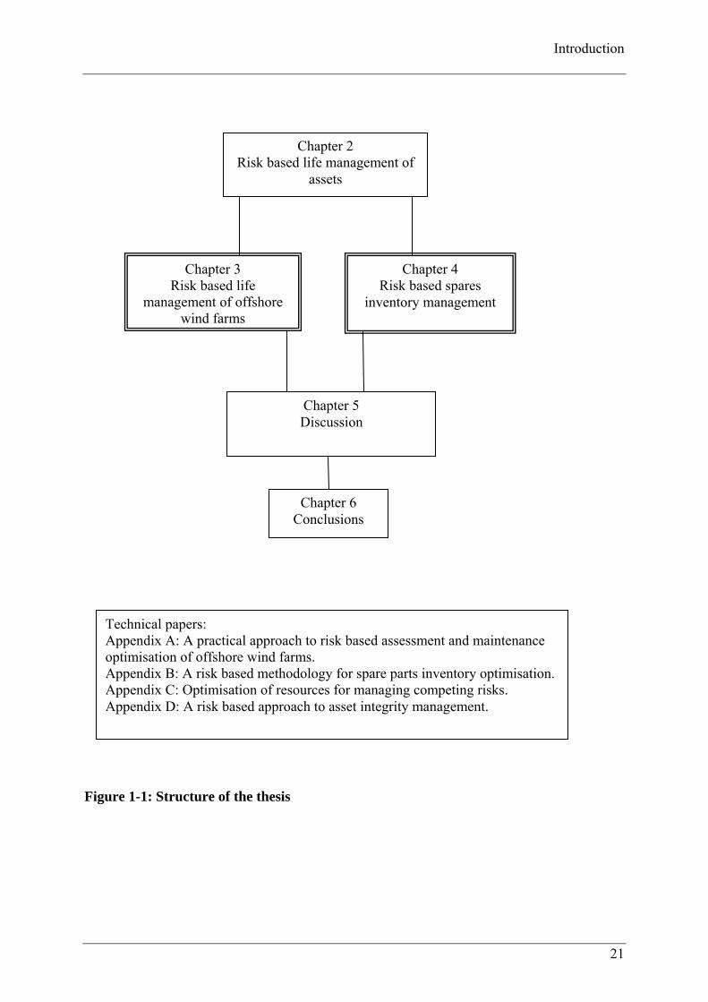
1.3 THE STRUCTURE
The structure of the thesis, chapter 2 onwards, is depicted in figure 1-1.

Introduction
17
Chapter 2 sets out the common risk based attributes of the methodologies described in the
sections that follow. It starts with introducing the terms and concepts used in this work: there
is a description of risk in its broadest sense; this is followed by a discussion on risk based
principles, life management of assets and the characteristics of offshore structures and
equipment.
It then discusses risk based approaches as applied to life management including the planning
of inspection and maintenance. The reasons why the bath tub curve, widely used in reliability
engineering, often with some modification, provides a theoretical framework for life cycle
management of assets is then discussed. The chapter refers to appendix E which contains
further details of topics mentioned in the text. Appendix F contains a discussion of the risk
matrix technique of qualitative risk analysis.
Chapters 3 and 4 describe two projects that are central to the research described in this thesis.
In figure 1-1, these are shown in highlighted boxes.
Chapter 3 describes parts of a project on risk based life management of offshore wind
turbines. This project developed a risk based life management methodology to find the
optimum trade-off between run-repair-replace costs and the expected cost of failure in
offshore wind farms, and produced prototype software to implement the same. In this
thesis, the focus of discussion is the risk based run-repair-replace decision-making
methodology aimed at maximising the net present value (NPV) of the investment. For
demonstration, the methodology has been applied to address corrosion of the tower
structure. There are two appendices referred to in Chapter 3.
o Appendix A is a paper on this project presented at the 2007 Offshore
Mechanics and Arctic Engineering (OMAE) Conference.
o Appendix G describes wind turbines.

Risk Based Life Management of Offshore Structures and Equipment
18
Chapter 4 describes a project to develop a risk based spares inventory management
system. In this project, a model for managing risk was developed to find the optimum
level of spares of different kinds a major industrial enterprise should advance order
given that failures requiring these may occur in service. The particular application was
a fleet of cargo ships where parts of different kinds are required to keep ships available
for service. There are two appendices relating to this project.
o Appendix B is a working paper presented at the 2008 International Mechanical
Engineering Congress and Exposition (IMECE), USA.
o Appendix C is a paper, describing further progress, presented at the 2009
Engineering Structural Integrity Assessment (ESIA-10) conference,
Manchester, UK.
Chapter 5 discusses the salient common features in the application of the risk based
approaches presented in the previous chapters and comments on their uptake and relevance.
The practical issues in applying the research and possibilities for further work are also
considered.
Chapter 6 sums up the thesis with concluding remarks.
1.4 OTHER RELEVANT STUDIES
The research presented here is directly or indirectly influenced by
Courses undertaken:
o MSc level course ‘Renewable Energy Technology’ at Cranfield University,
2006.

Introduction
19
o MSc level course ‘Structural Analysis’ conducted by Professor Silberschmidt
(completed Feb, 2008) at Loughborough University.
o ‘Research, Innovation and Communication’ module offered to doctoral
candidates at Loughborough University.
Conferences attended/ presented at:
o Attendance at ‘Using Probability Modelling in Structural Integrity
Assessments’ seminar organised by the Royal Academy of Engineering,
London, 9 June 2006.
o Attendance at ‘Risk Analysis and Structural Reliability’ course at
MARSTRUCT, Glasgow, and 20- 22 of November 2006.
o Conference presentation: Palisade Users’ conference, 23-24 April 2007,
London. Presentation titled ‘Monte Carlo Simulation (MCS) Technique for a
Probabilistic Implementation of Structural Engineering Procedures’.
o Conference paper presentation: ‘A Practical Approach to Risk Based Life
Management of Offshore Wind Farms’. ASME- Offshore Mechanics and
Arctic Engineering Conference, San Diego, 10-15 June 2007.
o Conference presentation: ‘Maximising Net Present Value of Investment in the
Maintenance of Assets’ at Palisade Users’ Conference, London 22-23 April
2008.
o Conference paper presentation: ‘A Risk Based Methodology for Spare Parts
Inventory Optimisation’, ASME IMECE conference, 3 -6 Nov 2008, Boston,
USA.

Risk Based Life Management of Offshore Structures and Equipment
20
o Conference paper presentation: ‘Optimisation of resources for managing
competing risks’, ESIA10- Engineering structural integrity assessment: present
goals- future challenges, 19-20 May 2009.
Supervision:
o Professors Vadim V Silberschmidt (Loughborough University) and John D
Andrews (previously at Loughborough University).
o John B Wintle (TWI Ltd) and Julian B Speck (previously with TWI Ltd).
1.5 INDUSTRIAL HOST: TWI LTD
TWI Ltd is the industrial host of this engineering doctorate. TWI Ltd is an independent, not -
for- profit distributing, membership-based, engineering research and consultancy
organisation. TWI's mission is to deliver world-class service in joining materials, engineering
and allied technologies to meet the needs of a global membership and its associated
community.
This research draws heavily on my work done within the Asset Integrity Management section
of the Structural Integrity Technology Group (SITG) at TWI Ltd, Cambridge where I have
been based. The Asset Integrity Management section provides a variety of services to the
petrochemical and process industry. These services include: providing consultancy for
optimising inspection and maintenance, implementing risk based management principles,
assessing fitness for service (FFS) against code requirements, and providing plant integrity
courses in FFS, Risk Based Inspection (RBI), degradation and repairs.
Introduction
21
Figure 1-1: Structure of the thesis
Chapter 2 Risk based life management of
assets
Chapter 3 Risk based life
management of offshore wind farms
Chapter 4 Risk based spares
inventory management
Chapter 5 Discussion
Technical papers: Appendix A: A practical approach to risk based assessment and maintenance optimisation of offshore wind farms. Appendix B: A risk based methodology for spare parts inventory optimisation. Appendix C: Optimisation of resources for managing competing risks. Appendix D: A risk based approach to asset integrity management.
Chapter 6 Conclusions

Risk Based Life Management of Offshore Structures and Equipment
22

Risk Based Life Management of Assets
23
2 RISK BASED LIFE MANAGEMENT OF ASSETS
2.1 FUNDAMENTAL CONCEPTS AND DEFINITIONS
2.1.1 THE NATURE OF RISK
Risk is an intangible concept. It can be looked at from various perspectives and has
connotations depending on the context in which it is used. From one perspective it is a
combination of the probability of harm and the severity of that harm (ISO/ IEC Guide
51:1999 1999).
A more encompassing description of risk is obtained by considering it to be inherent in any
action and, indeed, inaction. Many organizations increasingly apply risk management to
optimise the decisions regarding potential opportunities that need to be acted upon. In this
sense, risk has a broader meaning than mentioned above. The ISO/ IEC guide on risk
management vocabulary defines risk as the combination of the probability of an event and its
consequence (PD ISO/IEC Guide 73:2002 2002). The document notes that risk is generally
used only when there is at least a probability of negative consequences, and in some
situations, risk arises from the possibility of deviation from the expected outcome or event.
This description of risk is all including: most actions do have potentially negative
consequences; actions often assume normal conditions, deviations from which result in
outcomes that are different from what was expected. Where quantitative risk modelling is
involved, normal conditions may entail mean values (in statistical terms). Deviations from
normal, or the degree of (or the lack of) confidence in input values to the model, may depict
risk.

Risk Based Life Management of Offshore Structures and Equipment
24
In the context of this thesis, ‘risk’ is used in its broadest sense, to mean the combination of the
probability of an event and its consequence. The consequences are usually negative and
quantified in some way.
Risk is a complex entity: it cannot be measured easily as it involves probability and
prediction. There are two components to our inability to precisely determine risk- these are
variability and uncertainty in the inputs to risk analysis. Variability, also called as “aleatory
uncertainty” or “stochastic variability”, is the effect of chance and is a function of the system,
not reducible through further study or further measurement, but may be reduced by changing
the physical system. Uncertainty, also called as “epistemic uncertainty” or “fundamental
uncertainty” is the assessor’s lack of knowledge (level of ignorance) about the parameters that
characterise the physical system that is being modelled (Vose 2008).
The comment made in a political risk management context offers another perspective “There
are known knowns. These are things we know that we know. There are known unknowns.
That is to say, there are things that we know we don't know. But there are also unknown
unknowns. There are things we don't know we don't know” (Rumsfeld 12 February 2002).
Unknown unknowns are the result of total ignorance. Known unknowns can be construed as
knowing the variability in the inputs, at best, or, at least knowing that certain variables
affecting the outcome are likely to change in ways not easily foreseeable. Taleb calls
unpredictable events ‘Black Swans’ and suggests that instead of trying to predict them in
vain, we need to adjust to their existence (Taleb 2007).

Risk Based Life Management of Assets
25
2.1.2 MEASURES OF RISK
Whilst accepting that the inputs to risk analysis may not always be precise or definite or,
indeed, lacking (not available) or retrospectively (post-event) realised as missing (not
conceived of), this thesis does not dwell on the moot issues relating to forecasting or
prediction. Research presented here is more influenced by the study of the management of
risk than by the study of risk: the focus is on how to make the best use of available
information in the management of risks.
Probability or likelihood, mentioned above, is the extent to which an event is likely to occur.
Mathematically, probability is a real number between 0 and 1 indicating the occurrence of a
random event. It can be related to the long-run relative frequency of occurrence or to a degree
of belief that the event will occur. Degrees of belief about the likelihood of an even can also
be expressed in classes or ranks such as Very Low, Low, Medium, High and Very High.
Consequence is the outcome of an event (an occurrence of a particular set of circumstances).
Consequences can be positive or negative but are always taken as negative in a safety context.
As in likelihood or probability, consequences can be quantitative or qualitative.
In the context of this thesis, risk will involve the probability or the likelihood of failure of a
component or a system of components to fulfil its design purpose in a given time frame and
under given operating conditions. Where the two components of risk i.e. the likelihood and
the consequence of a failure event are quantitatively expressed, risk will be expressed in terms
of ‘expected loss’. Expected loss can be defined quantitatively as the product of the

Risk Based Life Management of Offshore Structures and Equipment
26
consequences (C) of a specific incident and the probability (P) over a time period or
frequency of its occurrence (Andrews, Moss 2002):
(2.1)
Qualitatively, a set of events can be graded depending on their likelihood and the impact of
their occurrence. The risk matrix technique, discussed later on, is mainly a qualitative one,
although it can have quantitative values.
The risk of an event, expressed qualitatively (High, Medium, Low, for example) or
quantitatively (in absolute terms), is often evaluated as relative to some other event. For
example, the risk (of death) posed by a particular surgery may be compared to the risk of
death by accident prevalent in the area; indeed, it may also be compared to the risk of not
undergoing surgery.
Risks here broadly fall in the following three categories: Occupational risks that impact
personnel engaged in industry; Societal risks that impact the people and the environment;
Financial risks that arise from loss of capital assets, production and compensation.
2.1.3 RISK MANAGEMENT
Risk management is coordinated activities to direct and control an organization with regard to
risk. It includes risk assessment which is the overall process of risk analysis and risk
evaluation. Risk analysis is the systematic use of information to identify sources of risk and to
estimate it. Risk evaluation is the process used to compare estimated risk against given risk
criteria to determine the significance of risk (API 2002a).
.PCR

Risk Based Life Management of Assets
27
2.2 ASSETS AND THEIR MANAGEMENT
2.2.1 OFFSHORE STRUCTURES AND EQUIPMENT
Ships and tankers, offshore oil rigs, sub sea pipelines and other offshore installations such as
FPSO (Floating Production Storage and Offloading) vessels, offshore CCS (Carbon Capture
and Storage/ Sequestration) depots are all offshore structures or equipment. These differ from
their counterparts on land in a number of ways: one crucial difference is that the nature of
risk, in terms of both the likelihood of failure and the consequences of the same, offshore is
different to that onshore.
Often offshore structures are complex, large and operate in a hostile environment. Without
life management, they are more susceptible to failure. At times they have a higher degree of
novelty than onshore structures. Some structures, for example, FPSO vessels, are often
converted ships not designed for this new purpose and need special attention; some of their
design aspects may be outside Class rules.
In terms of occupational risks, for serious crises personnel offshore have more limited escape
routes and need to rely on support from land that might not be forthcoming for a variety of
reasons. Societal risk, in case of offshore structures is usually restricted to the marine
environment. However, there are instances where pollution has affected people in coastal
areas. Breakdowns at sea often take longer to rectify: they may entail waiting for suitable
weather windows or dry docking a ship, for example. Thus there is often a prolonged period
of production loss leading to financial loss.
Risk Based Life Management of Offshore Structures and Equipment
28
The nature of risk for different structures differs: ships may be able to change course to avoid
extreme loading, whereas fixed structures such as oil rigs may be subject to more extreme
loading. Wind turbine structures are fixed but carry a rotating wind turbine adding to the type
of loading normally experienced by offshore structures. Some structures like oil rigs may
have a contingent of personnel whereas others such as wind farms are usually unmanned.
2.2.2 ASSET MANAGEMENT
Asset integrity management (AIM) includes all actions that enable an asset to perform its
function effectively and efficiently whilst safeguarding life and the environment. ‘Asset
integrity management ensures that the people, systems, processes and resources which deliver
integrity are in place, in use and fit for purpose over the whole life-cycle of the asset. The
objectives of an AIM system are the delivery of business requirements to maximise return on
assets, whilst maintaining stakeholder value and minimising business risks associated with
accidents and loss of production’ (Bureau Veritas).
There are various documents pertaining to the practice of AIM. In response to demand from
industry for a standard for asset management, there is a publicly available specification (PAS)
first published in 2004 and superseded in 2008. The document (BSI 2008) lists terms and
definitions, and provides a framework for AIM. Another good practice guide in asset
management is by CIRIA (Construction Industry Research and Information Association)
(CIRIA 2009).
The objectives of AIM mentioned above are typical in the engineering industry. As is evident,
AIM usually includes both safety and reliability driven risk management as well as
commercially driven risk management. This is in contrast to practices in the financial sector
where risk management is usually purely driven by commercial or business considerations
and indeed, the metrics used to measure such risk reflects this.

Risk Based Life Management of Assets
29
2.2.3 THE PRACTICE OF ASSET MANAGEMENT
The practice of asset integrity management is not new. However, it is only recently that it is
increasingly being recognized as a distinct set of business processes, disciplines and
professional practices. This recognition is in no small part due to the complexity of the assets
and the linkages between various asset systems created in industry- such systems require a
holistic/ integrated view for them to operate safely and efficiently.
Factors such as more experience in operating assets, a better understanding of failures, more
computing power to create and run sophisticated models, IT systems and better condition
monitoring techniques are helping in increasing the effectiveness of asset integrity
management.
Within asset management, there are strategies and techniques to implement these strategies.
For example, risk based inspection (RBI) is a strategy and some of the tools to implement this
strategy are simulation, HAZOPS, Probabilistic analyses, and FFS assessments. There are a
number of commercially available tools to provide inputs or to aid decision making in asset
management. For example, there are tools developed by Decision Support Tools Ltd such as
APT© (Asset Performance Tools) toolkits developed for Inventory and purchasing decisions,
maintenance/ inspection scheduling, etc.). SIL (Safety Integrity Level) assessments are formal
classification methods that provide a record of a quantified assessment of the probability of
failure on demand of a safety system taking into account the consequences of such failure.
SILs often form a part of a Quantitative Risk Assessment (QRA) that is then fed into a
decision-support tool. TWI has Riskwise© software aimed at implementing risk based
approaches (following various ASME/ BSI codes or bespoke practices) in the inspection and
maintenance of assets such as power plants, refineries and pipelines.
Risk Based Life Management of Offshore Structures and Equipment
30
The discussion above and in previous sections shows that asset management requires people
who can take a wider multi-disciplinary perspective. Apart from engineering knowledge and
skills, an awareness of the larger context in which an asset is operating is often required. As
pointed out by the Woodhouse Partnership, asset management needs skills such as reliability
and maintenance engineering, root cause failure analysis, life cycle costing, project/ change
management that have traditionally not been the focus of engineering degrees (The
Woodhouse Partnership Ltd, 2008). However, now distinct engineering disciplines such as
systems engineering, reliability engineering and operations management are dedicated to
looking at these aspects in greater detail.
2.2.4 LIFE MANAGEMENT OF ASSETS
‘Equipment or structure begins to age as soon as it is built. Cyclic stresses cause fatigue and
looseness. High temperature causes creep. Erosion and corrosion cause thinning and
weakening. Thus age in many ways degrades, deteriorates and destroys’ (ASME International
2003a).
Life management includes all processes that manage the ageing of assets during their life. The
HSE report on plant ageing (Wintle et al. 2006) segments ageing management into:
(a) Setting up an organizational structure to manage ageing
This includes taking responsibility for and control of the process of managing assets,
establishing a company culture, strategy, systems for knowledge management and retention,

Risk Based Life Management of Assets
31
and taking care of human factors such as competencies required, training, succession planning
etc.
(b) Identification of ageing
This includes establishing damage types and mechanisms, assessing the rate and accumulation
of damage, assessing age related risk factors, and inspection and non-destructive testing.
(c) Addressing ageing
This includes assessing fitness-for-service and remaining life. Fitness-for-service of an asset
is its adequacy to meet specified performance criteria for a period of continued service taking
into account degradation and other changes that may have occurred or that are postulated to
occur in future. Maintenance, repair and modifications, revalidation of equipment, planning
for spares, reviewing schemes of examination and condition monitoring, and determining the
end of equipment life, usually using a financial criterion, are also part of ageing management.
‘Ageing’ in the current context is the process of deterioration and damage taking place since
the equipment or structure was new. Ageing may not necessarily be a symptom of old age.
Relatively new equipment may have undergone more ageing than equipment that was put into
service earlier. Assessing ageing- knowing the current state of assets and assessing future
condition, bearing in mind the factors that influence the onset, evolution and mitigation of
degradation- is a very significant part of life management.

Risk Based Life Management of Offshore Structures and Equipment
32
Assessing ageing for life management poses challenges to those responsible for it: different
components (of a system) age differently and at a different rate; a single component may age
differently and at a different rate over a period of time; the consequences of failure of one
component may be different to those of another; and, different components may have
different costs and techniques associated with managing them. Thus there are competing risks
of failure and finite resources to manage them. Moreover, in certain situations, condition
monitoring and inspection, the two main inputs to risk analysis within life management may
not be achievable effectively and with precision.
Life management of assets is a critical activity: it can optimise performance within constraints
such as costs, reliability and safety. It has a direct bearing on the availability of assets for
production.
2.2.5 ROLE OF INSPECTION AND MAINTENANCE IN LIFE MANAGEMENT
It is necessary to assess Ageing to establish the state or condition of equipment that could
justify its continued service, re-rating, repair, or scrapping. Inspection provides information
regarding the current state of equipment. This information is helpful in reassessing risk. For
example, inspection may reveal that a particular damage rate is more than initially assumed in
a risk assessment leading to revised estimates. Inspection per se does not reduce risk: it is an
integral part of risk management that may lead to risk reduction by informing further action
such as maintenance and repair. The risk based inspection planning process followed by API
(API 2002b) is shown in figure 1-2.

Risk Based Life Management of Assets
33
Maintenance includes all activities that sustain or protect equipment for it to remain fit for
service. In terms of the bath tub curve discussed in the next section, maintenance prolongs the
useful life of equipment.
Figure 2-1: Risk based inspection planning process (API recommended practice 580)
2.2.6 DIFFERENT APPROACHES TO LIFE MANAGEMENT
Whilst there remains a need for traditional approaches to inspection and maintenance, it is
increasingly felt that more advanced approaches are required. This is mainly due to two
reasons:
(a) To reflect the complexity and innovation involved in the assets. It is often seen that there
are complex systems within systems with a lot of interaction between them. The innovation
within systems means that experience based information- the main input to time based
inspection and maintenance- is not available. For example, in the shipping industry, some
aspects of design may fall outside the remit of traditional Class rules (that are experience
based).
(b) To operate at an optimal level within the competitive pressures faced by asset managers.
Data and Information collection
Consequence of Failure
Probability of Failure
Risk ranking
Inspection plan
Mitigation (if any)
Reassessment

Risk Based Life Management of Offshore Structures and Equipment
34
The more advanced approaches, as opposed to the rule-based or time-based traditional
approaches, give operators some flexibility in the management of their assets whilst meeting
the same objectives. The flexibility is as a result of undertaking actions not on a fixed
schedule, but on factors such as the condition of the asset (symptoms of ageing). The risk
based approach uses risk based criteria to prioritize efforts and make the optimum use of this
flexibility.
Generally, in refining and chemical process plants, a relatively large portion of risk is
concentrated in a smaller percentage of equipment (API). It thus makes sense to focus
resources on the high risk components of a plant. It must be noted the development of such
condition based approaches to AIM has been aided, in no small measure, by advances in NDT
and information and communication technology.
Inspection and maintenance strategy have followed an evolutionary continuum from the more
time based traditional approaches to the advanced ones such as risk based (figure 2-2, adapted
from (Lee et al. 2006)).
Figure 2-2: Continuum of approaches leading up to risk based approaches
Time-based Condition- based
Risk based
Traditional approach
Rule or Standard based (rules based on experience and industry average conditions)
Prescriptive Regulatory enforced Calendar based
intervals ‘Preventive
Maintenance’
Inspection intervals/ Maintenance based on condition
‘Predictive Maintenance’- prediction based on condition
Priority accorded depending on the likelihood and the consequence of failure
Trade-off between inspection effort and risk involved
Proactive approach

Risk Based Life Management of Assets
35
The figure above shows some attributes of the main approaches to life management.
Time-based approaches are those in which specified action is required at some point of
time; often there are industry standards stipulating when or how frequent the action is
required. The approach is also called the rule-based approach as this approach is
prescriptive and the scheduling of the concerned action is not at the discretion of the
operator. These rules or standards are based on industrial experience and are
influenced by historical data; in this sense, the rules assume that the asset is operating
in industry-wide average conditions.
Condition-based approaches are those in which action is informed by the condition of
the asset. Relative to the rule-based approach, the approach here is more case-by-case,
i.e., based on current state of the asset and on local conditions.
The more advanced risk based approach prioritises action based on the risk profile of
various components within a system; the aim here is to focus resources on the
components that are deemed more risky. Relative to other approaches, this is a more
sophisticated approach to asset management in that, apart from factors considered in
the previous approaches, here the context in which the asset (or a component within a
system) is being operated is also considered.
Risk based approaches in a way often add a third dimension to failures. Apart from the
likelihood and consequence of failures, these approaches, by focussing resources on
high risk components, consider the manageability aspects of failures within resource
constraints. These approaches often answer the question: how to best manage the risk
from failures within a system of components, given the resources available?
In the interest of continuity, mention must be made of some other approaches, each having
their own bias. Reliability Centred Maintenance (RCM) is a subset of risk based maintenance

Risk Based Life Management of Offshore Structures and Equipment
36
in that maintenance is optimised taking into consideration the effect the equipment has on
plant reliability. Here, reliability can be quantitatively expressed as the probability that an
item (component, equipment, or system) will operate without failure for a stated period of
time under specified conditions. Reactive Maintenance (RM) is an approach in which
maintenance is performed only when the machine fails or shows signs of failing. Run-to -
failure policy is one in which the equipment is run until it breaks down effecting RM or
resulting in discarding the equipment, for example, a satellite.
The above discussion shows that the level of sophistication in various approaches to
maintenance (asset life management, in general) increases from the run-to-failure policy to the
risk based approach.
2.3 RISK BASED APPROACHES TO LIFE MANAGEMENT
2.3.1 BACKGROUND
Increased competition is a major driver for cost effective approaches to the life cycle
management of assets. One such approach is the risk based approach where ‘risk’ involves the
likelihood of failure of an equipment, component, or structure to fulfil its function and the
consequential impact of such a failure.
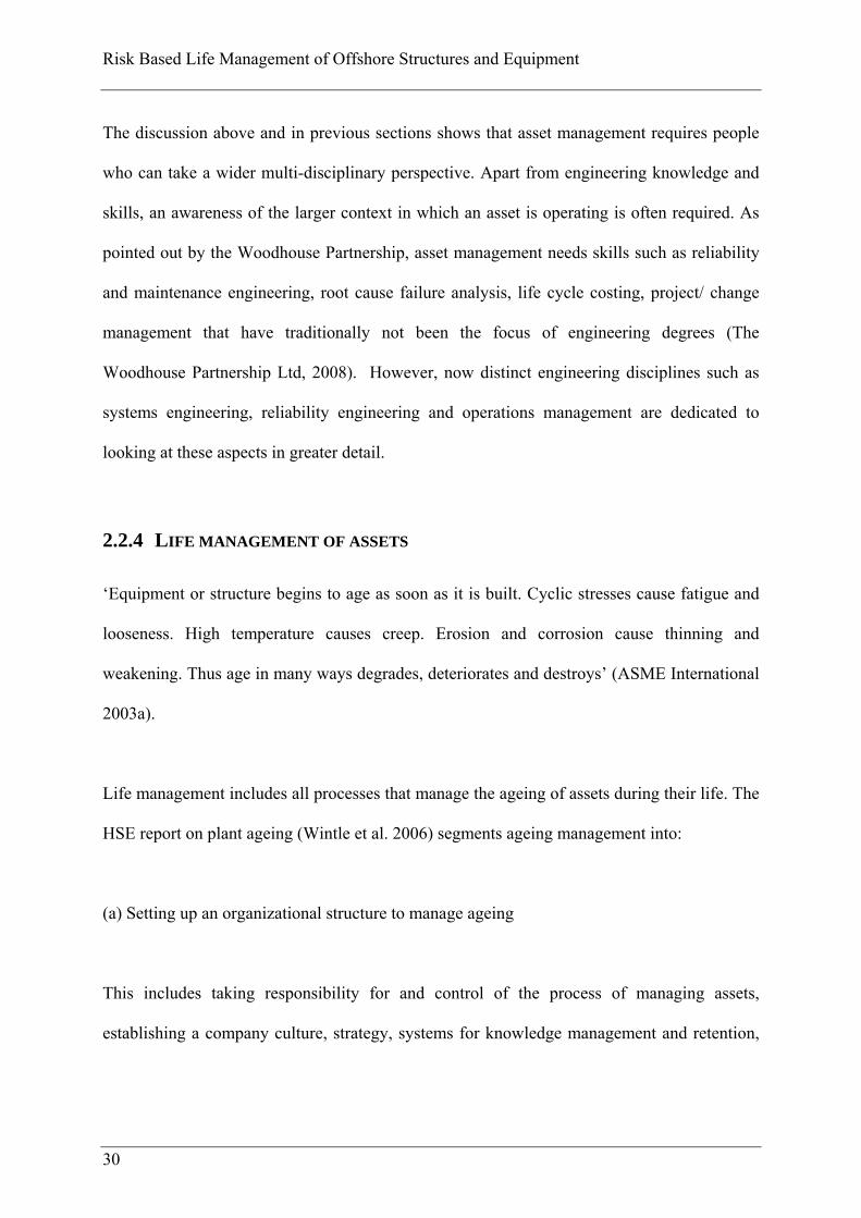
Life cycle management is particularly crucial for a plant in the Useful stage and the Ageing
stage of its life cycle as depicted in the classic bathtub curve shown in figure 2-3. Figures 2-4
and 2-5 have been adapted from the HSE report on plant ageing (Wintle et al. 2006). The bath
tub curve is the idealized curve of the failure rate within a system of infinite components
versus operating time. Depending on the failure rate, different phases can be discerned in the
Risk Based Life Management of Assets
37
lifetime of a system. There are no fixed demarcations between these stages. Indeed, two
systems commissioned together may be in different stages of their life cycle.
Stage 1: ‘Infant Mortality’
As a system is put into service, initially the failure rate is high because of the so called
‘teething’ problems (figure 2-3). The high failure rate during this stage could be because of
one or the combination of the following:
Figure 2-3: The bath tub curve and its components
---- Early ‘infant mortality failure’ rate .... Wear-out failure rate ___ Constant (random) failure rate Stage I: Infant mortality Stage II: Useful life Stage III: Ageing The curves in the figure do not use the same scale.
Fai
lure
rat
e
Operating life
Stage I Stage II Stage III Bath tub curve (Observed failure rate)
Risk Based Life Management of Offshore Structures and Equipment
38
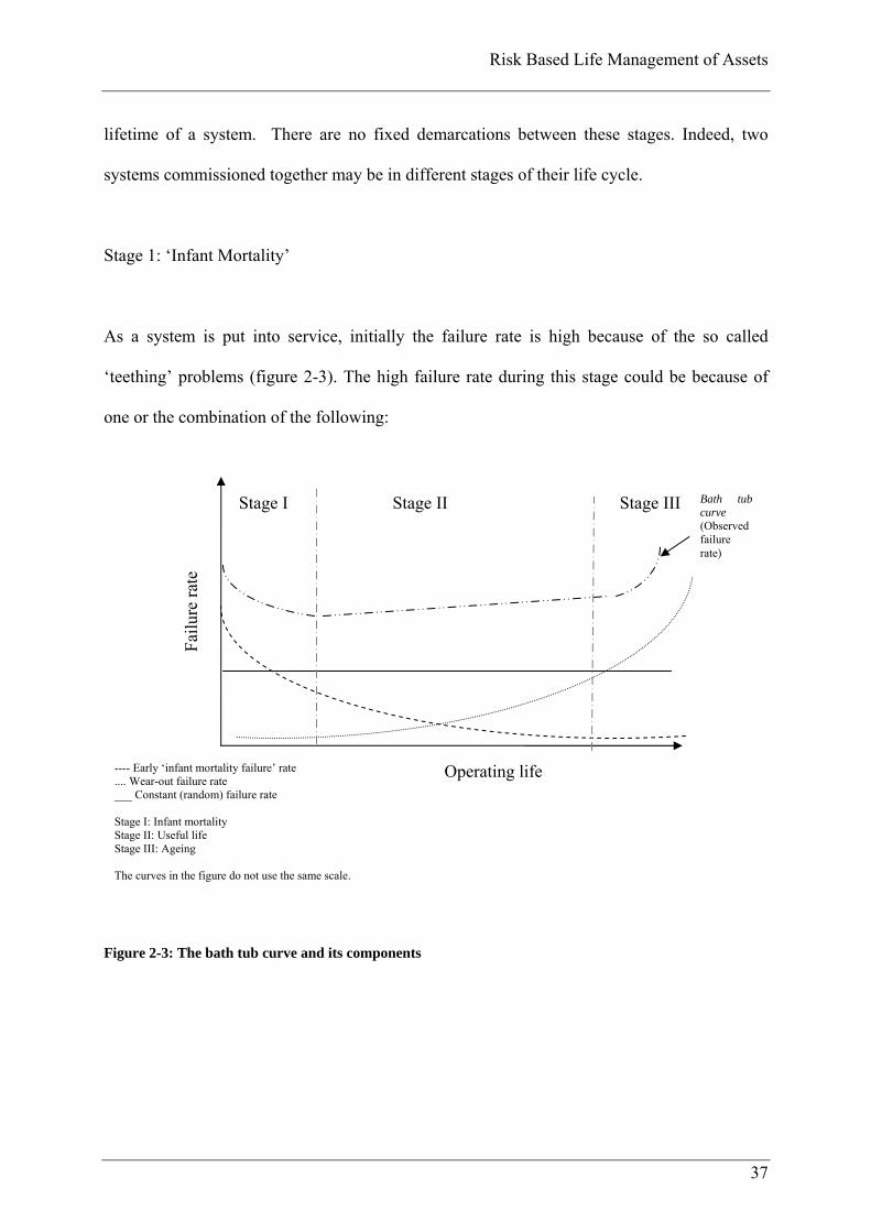
Figure 2-4: Variation in accumulated damage during equipment cycle
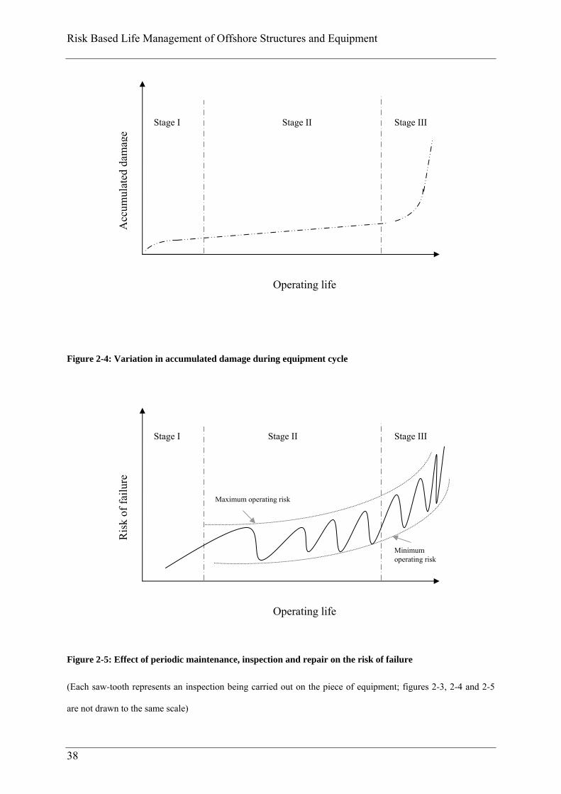
Figure 2-5: Effect of periodic maintenance, inspection and repair on the risk of failure
(Each saw-tooth represents an inspection being carried out on the piece of equipment; figures 2-3, 2-4 and 2-5
are not drawn to the same scale)
Ris
k of
fai
lure
Operating life
Maximum operating risk
Minimum operating risk
Stage I Stage II Stage III
Acc
umul
ated
dam
age
Operating life
Stage I Stage II Stage III
Risk Based Life Management of Assets
39
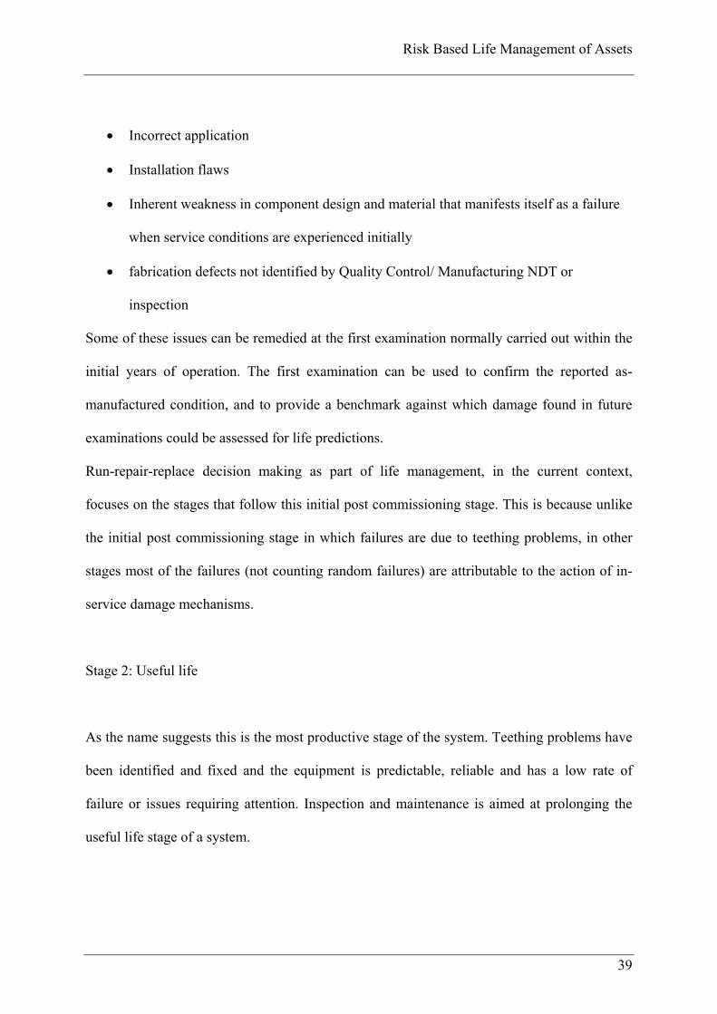
Incorrect application
Installation flaws
Inherent weakness in component design and material that manifests itself as a failure
when service conditions are experienced initially
fabrication defects not identified by Quality Control/ Manufacturing NDT or
inspection
Some of these issues can be remedied at the first examination normally carried out within the
initial years of operation. The first examination can be used to confirm the reported as-
manufactured condition, and to provide a benchmark against which damage found in future
examinations could be assessed for life predictions.
Run-repair-replace decision making as part of life management, in the current context,
focuses on the stages that follow this initial post commissioning stage. This is because unlike
the initial post commissioning stage in which failures are due to teething problems, in other
stages most of the failures (not counting random failures) are attributable to the action of in-
service damage mechanisms.
Stage 2: Useful life
As the name suggests this is the most productive stage of the system. Teething problems have
been identified and fixed and the equipment is predictable, reliable and has a low rate of
failure or issues requiring attention. Inspection and maintenance is aimed at prolonging the
useful life stage of a system.
Risk Based Life Management of Offshore Structures and Equipment
40
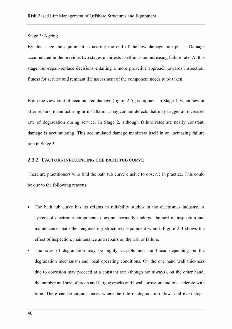
Stage 3: Ageing
By this stage the equipment is nearing the end of the low damage rate phase. Damage
accumulated in the previous two stages manifests itself in as an increasing failure rate. At this
stage, run-repair-replace decisions entailing a more proactive approach towards inspection,
fitness for service and remnant life assessment of the component needs to be taken.
From the viewpoint of accumulated damage (figure 2-5), equipment in Stage 1, when new or
after repairs, manufacturing or installation, may contain defects that may trigger an increased
rate of degradation during service. In Stage 2, although failure rates are nearly constant,
damage is accumulating. This accumulated damage manifests itself in an increasing failure
rate in Stage 3.
2.3.2 FACTORS INFLUENCING THE BATH TUB CURVE
There are practitioners who find the bath tub curve elusive to observe in practice. This could
be due to the following reasons:
The bath tub curve has its origins in reliability studies in the electronics industry. A
system of electronic components does not normally undergo the sort of inspection and
maintenance that other engineering structures/ equipment would. Figure 2-3 shows the
effect of inspection, maintenance and repairs on the risk of failure.
The rates of degradation may be highly variable and non-linear depending on the
degradation mechanism and local operating conditions. On the one hand wall thickness
due to corrosion may proceed at a constant rate (though not always), on the other hand,
the number and size of creep and fatigue cracks and local corrosion tend to accelerate with
time. There can be circumstances where the rate of degradation slows and even stops.

Risk Based Life Management of Assets
41
Corroding areas may build a layer of oxide that inhabits further attacks. Fatigue cracks
may stop growing for sometime if subjected to an overload.
A structure such as ship may age differently with a change in the operating condition: for
example, a change in cargo, or a change in route.
The manner of operation, maintenance, inspection and repairs has a bearing on the rate of
degradation. An asset may change hands, or maintenance personnel may change resulting
in a change in the manner an asset is operated and maintained. Invasive work can
introduce contaminants into the system thereby increasing the rate of degradation,
temporarily or in the long run. Appropriate inspection, maintenance and repairs of
damaged areas can reduce both the amount and the rate of change, while unnecessary
work may have little benefit.
Notwithstanding the above factors, in the life cycle management of assets, it is often useful to
assume that damage will accumulate over time and manifest itself in terms of an increasing
failure rate (figures 2-3, 2-4 and 2-5). This provides a theoretical framework on which to build
a strategy for asset management. It is worth noting here that wear (accumulating as a function
of hours of use, severity of use, and level of preventive maintenance) and deterioration (the
gradual decay, corrosion, or erosion as a function of time and severity of exposure conditions)
of an asset are major factors leading to the loss in value of the same over a period of time
(Collier, Glagola 1998). In accountancy, this loss of value is represented by depreciation of
the asset over the time. Thus, during the ageing phase of an asset, and at times the useful
phase, run-repair-replace decisions typically consider not just FFS assessments, but also
financial implications such as the cost of equipment failure, the cost of new equipment and
the depreciation (in accountancy terms) calculated on the asset. The model in the next chapter

Risk Based Life Management of Offshore Structures and Equipment
42
considers these factors in the run-repair-replace decision making in the management of
offshore wind farms.
Risk based maintenance approaches focus mainly on the useful and the ageing phases of a
system. The assessment of risk forms part of what is known as asset management as discussed
in chapter 1. The aim of risk based asset management is to assist companies in adopting a
holistic approach to improve performance, dealing not only with the technical or commercial
risks themselves but also the context in which they exist.
2.3.3 THE CONCEPT OF TARGET RISK/RELIABILITY LEVELS
Activities such as inspection, maintenance and repair aim at maintaining assets within
identified acceptable risk/ reliability levels. Figure 2-6 shows the main approaches to
establishing what acceptable level of risk / reliability is.
Figure 2-6: The approach to establishing acceptable risk/reliability levels
Acceptable probability of failure or Target risk/ reliability levels
1) Agree upon reasonable value
in cases of novel structures
2) Calibrate levels implied in currently
successful design codes 3) Minimise total expected cost over service life of the structure – used mainly for
failures resulting in economic consequences

Risk Based Life Management of Assets
43
The first approach can be based on expert-opinion elicitation for want of real data or
experience in operating the new type of structure/ equipment. There are formal procedures for
doing this (O’Hagan, Anthony et al, 2006; Ayyub, Bilal M, 2001).
The second approach, i.e. calibration to existing successfully used design codes, is the most
commonly used approach as it provides the means to build on previous experiences (Ayyub,
Bilal M., 2003). For example target reliabilities can be established by assessing those implied
in current codes or rules provided by classification bodies and industry societies in similar
applications.
The third approach is based on finding the optimum trade-off between the economic costs of
an action that mitigates risk and the cost (risk of failure) without that action. Here the aim is to
minimise the total ‘expected cost’ of operating a plant (structure/ equipment). The next
chapter shows how ‘expected cost’ is a useful measure of risk.
The approaches are by no means always mutually exclusive in their application. The risk
based approaches described in the following chapters aim to minimise expected costs while
remaining within certain constraints including stipulated reliability/risk levels.
2.3.4 GENERAL METHODOLOGY FOR RISK BASED LIFE MANAGEMENT
This section discusses main features of a typical Risk based Life Management (RBLM)
approach which includes the following:
System analysis
Qualitative risk assessment
Quantitative risk analysis
Risk Based Life Management of Offshore Structures and Equipment
44
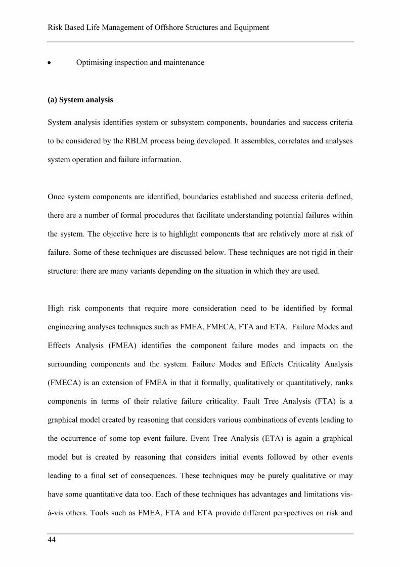
Optimising inspection and maintenance
(a) System analysis
System analysis identifies system or subsystem components, boundaries and success criteria
to be considered by the RBLM process being developed. It assembles, correlates and analyses
system operation and failure information.
Once system components are identified, boundaries established and success criteria defined,
there are a number of formal procedures that facilitate understanding potential failures within
the system. The objective here is to highlight components that are relatively more at risk of
failure. Some of these techniques are discussed below. These techniques are not rigid in their
structure: there are many variants depending on the situation in which they are used.
High risk components that require more consideration need to be identified by formal
engineering analyses techniques such as FMEA, FMECA, FTA and ETA. Failure Modes and
Effects Analysis (FMEA) identifies the component failure modes and impacts on the
surrounding components and the system. Failure Modes and Effects Criticality Analysis
(FMECA) is an extension of FMEA in that it formally, qualitatively or quantitatively, ranks
components in terms of their relative failure criticality. Fault Tree Analysis (FTA) is a
graphical model created by reasoning that considers various combinations of events leading to
the occurrence of some top event failure. Event Tree Analysis (ETA) is again a graphical
model but is created by reasoning that considers initial events followed by other events
leading to a final set of consequences. These techniques may be purely qualitative or may
have some quantitative data too. Each of these techniques has advantages and limitations vis-
à-vis others. Tools such as FMEA, FTA and ETA provide different perspectives on risk and

Risk Based Life Management of Assets
45
are not competing tools; they often act in conjunction with each other to give a larger picture
of risk. Appendix E gives more details about the techniques discussed above.
(b) Qualitative risk analysis
Qualitative risk analysis is a technique of setting priorities by risk ranking system components
into broad failure likelihood and consequence bands. The rankings are relative and based on
the risk perception gained by experience or historical data captured by formal engineering
techniques such as FMEA, FMECA, FTA and ETA as discussed above. Qualitative
assessment creates a risk matrix that enables decision-makers to focus on highest risk for
further action. This is the first step in thinking in terms of risk rather than just the probability
or consequence of failure in isolation. Again, as it is a qualitative assessment, consequences
like safety and environmental damage that are not easily quantifiable, may be factored in.
This stage will act as a screening stage focusing any further quantitative assessment on the
higher risk components.
Appendix F describes the risk matrix technique which is a common qualitative risk analysis
technique. In the appendix some variants of the risk matrix are also discussed- these are semi-
quantitative risk assessments.
(c) Quantitative analysis
Quantitative analysis replaces to the maximum possible extent, the qualitatively assessed
likelihood and consequence estimates with numerical failure probability and consequence cost
values.

Risk Based Life Management of Offshore Structures and Equipment
46
Quantitative analysis is an elaborate exercise and is usually undertaken only to analyse those
components that are identified as high risk by qualitative analysis. Whilst consequence cost is
relatively easy to quantify - in terms of repair/replacement cost, loss of revenue, etc., the
likelihood (or probability) of failure of an asset over time is more complex to ascertain.
Failure probability assessment is usually obtained from:
1. Specific failure data – data that is class specific or plant specific and is locally
available. It may be the best source but may not be available and/or statistically
significant.
2. Generic failure data - available from OEMs and industry experts, reflecting average
operating conditions.
3. Engineering analysis - Remaining life estimates using deterministic and
probabilistic engineering tools.
The quantitative analyses in the chapters that follow use mainly engineering analyses and
generic data to arrive at the probability of failure of an asset over a period of time. Indeed,
there are techniques such as those based on Bayesian statistics that can be used to combine or
update data from various sources.
(d) Optimising inspection and maintenance
Optimising inspection and maintenance within RBLM involves finding the optimum trade off
between the cost of undertaking an action (inspection, maintenance, repair or replace) and the
risk of not taking that action expressed quantitatively in monetary terms or semi-
quantitatively. The optimisation shown in the following chapters takes into account
constraints such as the available budget, acceptable risk and reliability.
Risk Based Life Management of Assets
47
The chapters that follow have the same underlying theme- risk based optimisation in the life
management of assets. Risk, as mentioned earlier, involves the likelihood of failure and the
consequence of the same. Optimisation is finding the optimum trade off between the expected
cost (the risk) of failure and the cost of mitigating that risk within user specified constraints
such as acceptable risk level and the budget available.
Risk can be reduced to a specified acceptable risk level by reducing the likelihood of failure
or the consequences of such a failure. This reduction or mitigation is achieved at a cost which
in practice needs to be within a specific budget.
Risk based optimisation of a system is different to that of an individual component. Some risk
values of individual components may rise when the system risk is optimised. Indeed, if a
maximum acceptable risk value for each component is specified, then the system risk can be
optimised such that both individual and the overall system risks are within acceptable levels.
The chapter on optimising spares inventory contains more details regarding system and
individual risks.
The risk based optimisation in chapter 3 is aimed at finding the optimum time of repairing or
replacing an asset such that costs of doing so are balanced by the risks of not doing so.
The risk based optimisation in chapter 4 is aimed at maintaining an inventory of spares at an
optimum level by considering the costs of stocking spares and the costs of failure to meet a
demand for the spares.

Risk Based Life Management of Offshore Structures and Equipment
48
Project 1: Risk Based Life Management of Offshore Wind Farms
49
3 PROJECT 1: RISK BASED LIFE MANAGEMENT OF
OFFSHORE WIND FARMS
3.1 GENERAL APPROACH
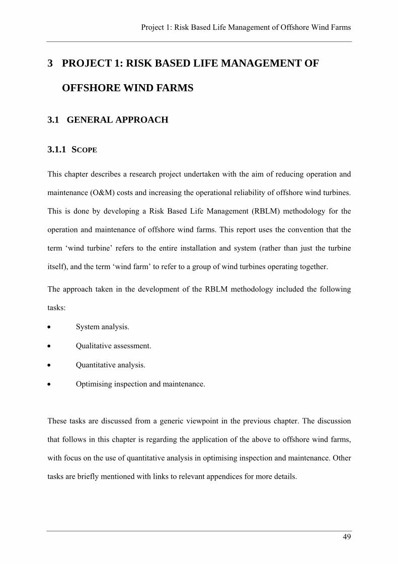
3.1.1 SCOPE
This chapter describes a research project undertaken with the aim of reducing operation and
maintenance (O&M) costs and increasing the operational reliability of offshore wind turbines.
This is done by developing a Risk Based Life Management (RBLM) methodology for the
operation and maintenance of offshore wind farms. This report uses the convention that the
term ‘wind turbine’ refers to the entire installation and system (rather than just the turbine
itself), and the term ‘wind farm’ to refer to a group of wind turbines operating together.
The approach taken in the development of the RBLM methodology included the following
tasks:
System analysis.
Qualitative assessment.
Quantitative analysis.
Optimising inspection and maintenance.
These tasks are discussed from a generic viewpoint in the previous chapter. The discussion
that follows in this chapter is regarding the application of the above to offshore wind farms,
with focus on the use of quantitative analysis in optimising inspection and maintenance. Other
tasks are briefly mentioned with links to relevant appendices for more details.

Risk Based Life Management of Offshore Structures and Equipment
50
A paper titled ‘A practical approach to risk based assessment and maintenance optimisation of
offshore wind farms’ presented at ASME’s Offshore Mechanics and Arctic Engineering
(OMAE) conference, June 10-15, 2007, San Diego, USA is attached as Appendix A.
3.1.2 SYSTEM DESCRIPTION AND ANALYSIS
The task started with understanding wind turbines. This included tracing the evolution of
modern wind turbines, identifying key components, and looking at recent development in
wind turbines. The task involved (1) conducting a literature review, (2) surveying wind
turbine reliability databases and (3) eliciting expert opinion.
Appendix G describes a review of literature to understand wind turbines.
The survey of wind turbine reliability databases (an exercise that included processing of data
to extract relevant failure statistics) and the elicitation of expert opinion - experts from OEMs
and wind turbine operators - is the topic of a confidential report not included in this thesis.
However, an overview of publicly available reliability databases that were considered in the
report is given below.
The survey of wind turbine reliability databases included the following:
i) WindStats:
WindStats Newsletter is a quarterly wind energy publication with news, reviews on wind
turbine production and operating data from over 15,000 wind turbines. It publishes production
and failure data of wind turbines from Denmark, Sweden and Germany.
ii) The REISI (Renewable Energy Information System on Internet) database from ISET
(Institute fur Solare Enertieversorgungstechnik), University of Kassel, Germany in
conjunction with ‘Wind Energy Report Germany 2005):

Project 1: Risk Based Life Management of Offshore Wind Farms
51
ISET manages a central data base containing wind turbine operating data (from wind turbines
funded under a project called ‘250 MW Wind’, and data from other turbines that is voluntarily
reported).
The data collected and processed by ISET is commercially available for the benefit of wind
turbine operators and other interested parties. The Wind Energy Report Germany is the 15th of
the annually published operational results from the WTs included in the 250 MW Wind
funding programme. The programme initially started as 100 MW Wind programme in 1989
and was later expanded to 250 MW in 1991. By 1996, 1500 WTs with a total rated capacity of
350 MW were included in the programme. This programme provides one of the most
comprehensive long- term operating databases in the world. The WMEP aims to collect data
in a statistically useful way and evaluate it using uniform criteria for the benefit of the wind
energy sector in Germany and elsewhere.
iii) Data from Landwirtschaftskammer Schleswig-Holstein
In this database, output data and failures of all turbines in the Schleswig-Holstein province of
Germany are collected and presented. Data from about 500 turbines (57% of which are larger
than 500kW) for the years 1999 and 2000 was extracted from the publicly available DOWEC
project report (DOWEC).
iv) Caithness wind farm information forum
The forum (Caithness, date unknown) lists documented cases of wind turbine “accidents” that
are found and confirmed through press reports or official information releases from the 1970s
till recently.
v) Information from ‘Guidelines on the environmental risk of wind turbines in the
Netherlands’

Risk Based Life Management of Offshore Structures and Equipment
52
This report (Braam, Rademakers, 2002) analyses over 200 severe incidents and accidents
from Denmark, Germany and the Netherlands. The data represents about 43,000 turbine years
and calculates the frequency of occurrence of events relevant to risk assessment.
The task resulted in identifying main components of wind turbines and parts more prone to
failure and/ or having relatively higher consequence of failure. However, formal
categorisation of components depending on their risk of failure took place in the next step.
3.1.3 QUALITATIVE ASSESSMENT
A qualitative risk assessment method specifically for wind turbine towers is captured in
spreadsheet format, screenshots of which can be seen in the figures accompanying the text.
The procedure for qualitative assessment is described below.
Table 3-3 presents a list of the main components that construct a wind turbine. The list,
which can be customized for specific wind turbine designs, is created by conducting system
analysis (as discussed above).
Each of the identified components are individually considered and ranked in qualitative terms
based on two criteria i.e. the likelihood of failure and the severity of the consequence of
failure. Various factors contributing to the likelihood of failure and consequences are
considered to get an overall likelihood factor and consequence ranking in qualitative terms.
Many of these factors can be assessed using techniques such as FMEA, ETA and FTA that
have been discussed in the previous chapter and/or referred to in the Appendices.

Project 1: Risk Based Life Management of Offshore Wind Farms
53
Factors contributing to the failure likelihood include:
Current condition of the component;
Design life consumed;
Number of active damage mechanisms;
Estimated rate of damage;
Efficiency of inspection;
Loading conditions;
Environmental conditions.
Factors contributing to the consequence of a failure include:
Production loss (during downtime);
Secondary damage (knock-on effects);
Threat to personnel;
Rectification costs;
Impact on reputation;
Redundancy.
This estimate is in qualitative terms and ranks from very low (VL) to very high (VH).
(VL-very low, L- low, M medium, H- high and VH- very high) More ranks could be used to
give the assessment further resolution if required. Likewise, more factors perceived to be
affecting the ranking could be added to the work sheet.
A possible qualitative ranking scheme for estimating the failure probability for a component is
shown below:
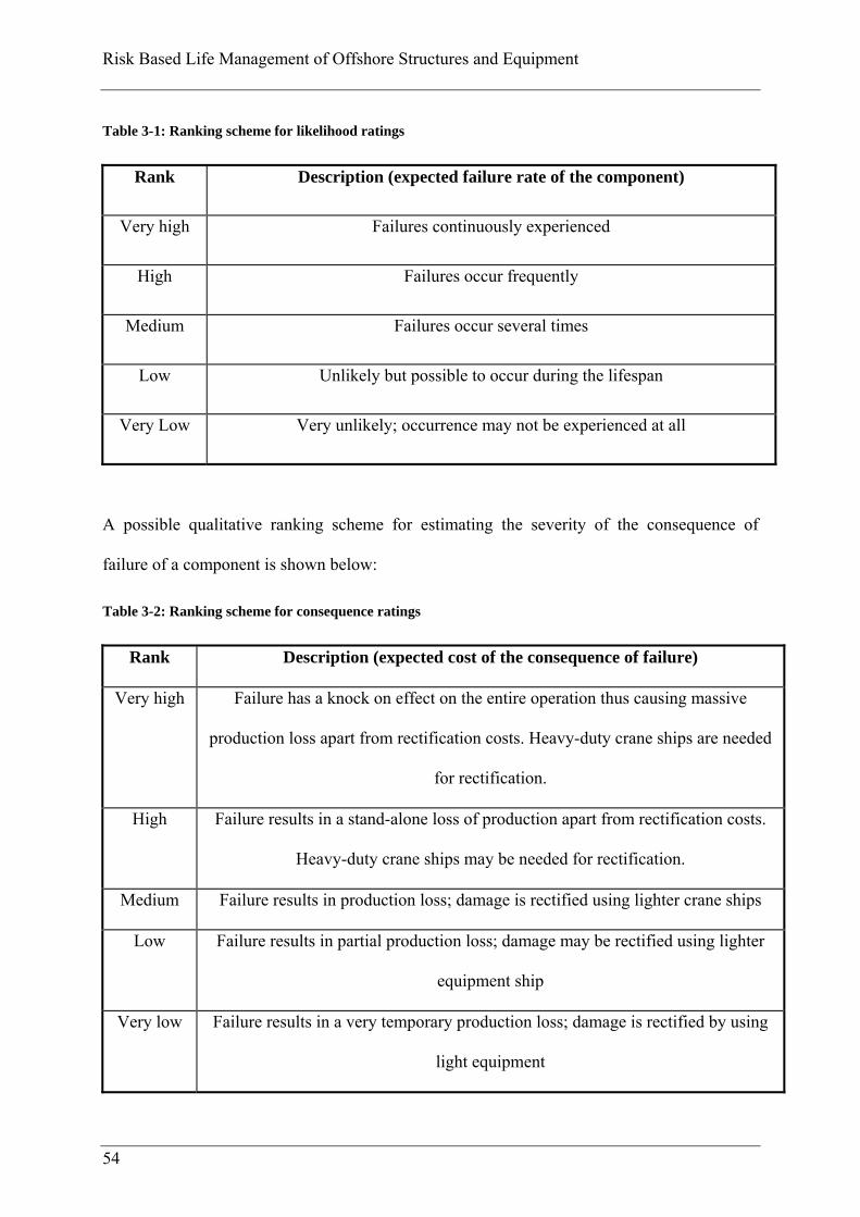
Risk Based Life Management of Offshore Structures and Equipment
54
Table 3-1: Ranking scheme for likelihood ratings
Rank Description (expected failure rate of the component)
Very high Failures continuously experienced
High Failures occur frequently
Medium Failures occur several times
Low Unlikely but possible to occur during the lifespan
Very Low Very unlikely; occurrence may not be experienced at all
A possible qualitative ranking scheme for estimating the severity of the consequence of
failure of a component is shown below:
Table 3-2: Ranking scheme for consequence ratings
Rank Description (expected cost of the consequence of failure)
Very high Failure has a knock on effect on the entire operation thus causing massive
production loss apart from rectification costs. Heavy-duty crane ships are needed
for rectification.
High Failure results in a stand-alone loss of production apart from rectification costs.
Heavy-duty crane ships may be needed for rectification.
Medium Failure results in production loss; damage is rectified using lighter crane ships
Low Failure results in partial production loss; damage may be rectified using lighter
equipment ship
Very low Failure results in a very temporary production loss; damage is rectified by using
light equipment

Project 1: Risk Based Life Management of Offshore Wind Farms
55
Table 3-3: Qualitative risk ranking
Component Likelihood Consequence Risk Score
RPM
Elec Control High Medium 48
Gear Box Low Very High 40
Yaw System Low Medium 24
Entire Turbine Low Very High 40
Generator Medium High 48
Hydraulic Low High 32
Grid Connection Medium Low 24
Blades Medium Medium 36
Brakes High Medium 48
Axle/ Bearing Medium Medium 36
Mech Control High Medium 48
Entire Nacelle Medium Medium 36
Coupling Medium Medium 36
Tower collapse Medium High 48
Foundation Low Very High 40
For simpler systems it is possible to plot the risk on a risk matrix (discussed in Appendix F) in
terms of the items assigned likelihood and consequence ratings as shown in the second and
third columns of table 3-3. Usually systems are more complex and additional steps are
required to assess risk. The next step imparts more discrimination to the risk assessment
procedure used for complex systems such as wind turbines.
The product of normalised numerical values for likelihood and consequence of failure gives a
risk priority measure (RPM) or a risk score. This is shown in table 3-3, 4th Column.

Risk Based Life Management of Offshore Structures and Equipment
56
RPM= (Normalised value of likelihood of failure) x (Normalised value of consequence of
failure)
The process of normalization is as follows:
If VL, L, M, H and VH can be represented by 20,40,60,80 and 100, then the risk profile of an
item, say the yaw system in table 3-3 above, which is ranked Low (40) on likelihood and
Medium (60) on the consequence of failure, can be represented as
24100/)60*40( ,
where 24 is the RPM of the yaw system. It must be noted here that these values are relative
values.
A histogram uses the RPMs to prioritize components in terms of their risk and thereby
highlight those components that need more attention, see figure 3-1.
Figure 3-1: Risk histogram
As shown in the figure, the collapse of the tower is in itself not a frequent event, but the risk
(RPM value 48) from such an event arises from the severity of the consequence. The blades of
a wind turbine have a high likelihood of being damaged, but the consequence severity is not
so high and hence the risk of such an event is less than that from a collapse of tower. (RPM
Risk Histogram using Risk Priority Measure (RPM)
0
20
40
60
Elec C
ontro
l
Gear B
ox
Yaw S
yste
m
Entire
Tur
bine
Gener
ator
Hydra
ulic
Grid C
onne
ction
Blades
Brake
s
Axle/ B
earin
g
Mec
h Con
trol
Entire
Nac
elle
Coupli
ng
Tower
Found
ation
Component number
RP
M

Project 1: Risk Based Life Management of Offshore Wind Farms
57
value 36). The values here are for demonstration only. In certain areas, for example in the
vicinity of human inhabitation or plant and machinery, the risk to life/ property posed by
pieces of damaged blade flying off may be considerable.
3.2 QUANTITATIVE ANALYSIS OF WIND TURBINE TOWER
3.2.1 CONCEPT
As seen in the previous section, a qualitative risk assessment helps maintenance personnel to
focus on high-risk components for further action. The next stage is to, as far as is practicable,
conduct a quantitative risk analysis of the component(s) identified as being high risk.
Quantitative analysis raises the decision making tool to a higher level of precision and risk
discrimination.
Quantitative analysis replaces the qualitatively assessed VL-VH failure likelihood and
consequence estimates with a numerical failure probability and a numerical consequence
value, usually represented by cost (£, $ etc.). For example, if the failure probability of a
structure is 0.05 per year and the consequence cost of such a failure is £ 100,000, then risk in
quantitative terms is the expected consequence cost should the failure of the structure occur,
Risk (£/ year) = (Probability of Failure) x (Consequence cost of the failure)
= (0.05) x (100,000)
= 5000.

Risk Based Life Management of Offshore Structures and Equipment
58
It must be noted that although not explicitly mentioned here or elsewhere, the failure
probability considered above and in the wider context of this thesis is, in fact, a joint
probability. It is, in effect, not just the probability of failure but the probability of a failure
leading to the specific consequence in consideration. For example, consider a container
containing an inflammable fluid being assessed. Assume that there is only one type of failure
i.e. ‘Loss of containment’ leading to only two possible consequences- ‘No fire’ and ‘Fire’- as
shown in figure 3-2. Then,
Figure 3-2: The probability of occurrence of a specific consequence
Probability of fire = (The probability of failure) x (The probability of ignition) (3.1)
Here, the probability of fire is a joint probability and not just the probability of failure. In the
discussion here, unless indicated otherwise, the probabilities are probabilities of failure
leading to the specific consequence under consideration.
A quantitative analysis could have deterministic values, a range of values or a distribution to
reflect the underlying uncertainty as input. A stochastic process is a process with an
Loss of containment (Probability of failure)
No fire (Probability of non-ignition)
Fire (Probability of ignition)
Project 1: Risk Based Life Management of Offshore Wind Farms
59
indeterminate or random element as opposed to a deterministic process that has no random
element. In a stochastic process, inputs and/ or outputs are a distribution of values described
by a probability function. For example, corrosion rate in a deterministic model may be
0.3mm/year, whereas in stochastic model would be, say, a normal distribution, N (.3, 0.05)
with mean 0.3 mm/year and a standard deviation of .05 mm/year. Most damage mechanisms
are stochastic in practice and need to be evaluated as such.
3.2.2 PROBABILISTIC REMAINING LIFE METHODOLOGY
Failure probabilities are difficult to ascertain. There are a number of methods to obtain failure
probability versus time data:
a) Using specific failure information: One method is to use specific failure data that is
plant, equipment or component specific, and is gathered from local sources such as
maintenance and inspection histories. This is usually the best source of information because it
is specific to local operating conditions such as weather, management strategy etc. However,
such failure data may not be available, or if available, may not be statistically significant.
Specific failure information can also be generated from industry experts
b) Using generic failure data: This data is obtained from original equipment
manufacturers (OEMs), industry experts or public sources. In a way, it is a collection of
specific information. Although such a data set represents a range of operating conditions
across a larger population of equipment, it is an excellent point of reference. The data is
statistically more significant as it is taken from a bigger population of equipment across
industries. Such databases exist in the Oil & Gas, power generation and aviation industries.
Risk Based Life Management of Offshore Structures and Equipment
60
c) Conducting engineering analysis: There are methods for predicting damage rates and
these can be incorporated in probabilistic models to calculate probabilities of failure.
The procedure here considers engineering analysis to demonstrate the technique of using
quantitative analysis as input to a risk model. A measurable degradation mechanism-
corrosion- has been chosen for which a probabilistic degradation model has been created. A
typical asset remaining life (RL) calculation has statistical distributions describing the damage
rate, the materials properties and the current damage state. These distributions are inputs to
the life calculation. In the technique described here, by using Monte Carlo Simulation (MCS)
software, random values are selected from each input distribution. The calculation is repeated
many times selecting random combinations of values from all inputs. Instances in which RL
is negative are counted as failure to calculate the probability of failure. The sections that
follow discuss the RL model further.
A failure modes and effects analysis identified corrosion, fatigue and scouring as the
significant degradation mechanisms affecting WT towers. The rate and action of these
degradation mechanisms can be quantified in terms of a probabilised damage model and
loading environment based on some assumptions. This quantitative assessment of failure
probability can then be used as input into a model for optimising inspection and maintenance.
In this work a risk model has been developed for corrosion but similar models could be
developed for fatigue and scouring. A full analysis would take all these mechanisms into
account. However, this work serves to illustrate the general approach.

Project 1: Risk Based Life Management of Offshore Wind Farms
61
3.2.3 DEGRADATION MECHANISMS
From the failure modes and effects analysis the following mechanisms causing degradation to
a WT tower structure were identified and are now discussed.
(a) Fatigue
The tower structure of a wind turbine is subjected to cyclic stresses causing fatigue. These
stresses originate from sources including variations in the wind loading, the effects of waves
and vibration induced by the movement of the turbine itself. The cyclic stresses cannot be
easily calculated since the loads are not well defined, but an alternative is to measure the
strain, or better still the fatigue damage, directly using strain gauges or a fatigue sensor
system.
There are a number of fatigue sensor systems in the market to assess fatigue in welded joints,
which are the areas most susceptible to fatigue. One such sensor- CrackFirstTM - developed in
a project funded by the DTI’s LINK Sensor and Sensor Systems for Industrial Applications
Programme is briefly discussed here. (More information is available at
http://www.strainstall.com/.)
The fatigue sensor is installed on a welded steel structure. It indicates the portion of fatigue
design life of the structure consumed. The sensors are so placed that they are subjected to the
same loading history as the structure they are monitoring. They record the cumulative fatigue
damage of the structure and thus enable engineers to estimate its remaining life.
There are several ways of powering and interrogating the sensor. For remote locations, such
as offshore wind farms, an on-board electronics unit that checks the sensor status and records
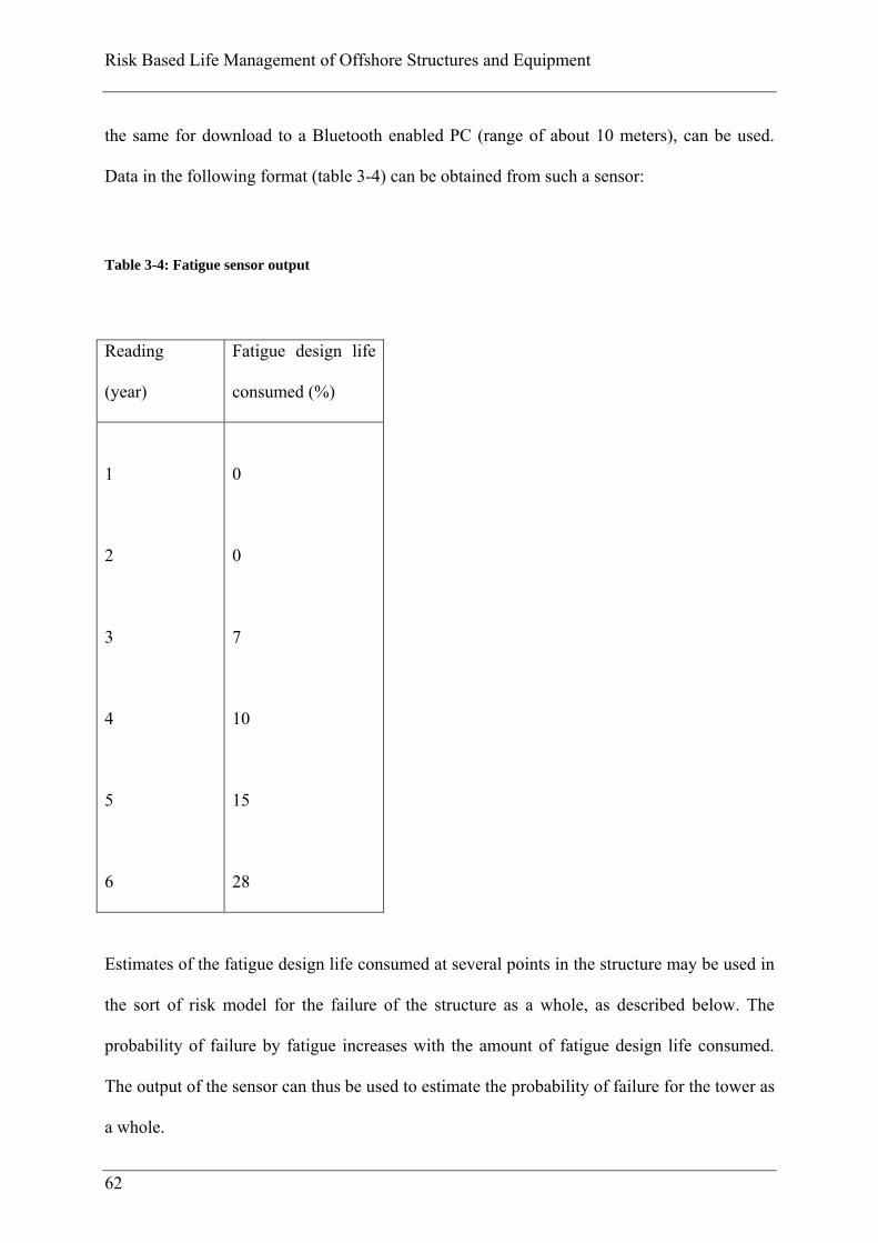
Risk Based Life Management of Offshore Structures and Equipment
62
the same for download to a Bluetooth enabled PC (range of about 10 meters), can be used.
Data in the following format (table 3-4) can be obtained from such a sensor:
Table 3-4: Fatigue sensor output
Reading
(year)
Fatigue design life
consumed (%)
1
2
3
4
5
6
0
0
7
10
15
28
Estimates of the fatigue design life consumed at several points in the structure may be used in
the sort of risk model for the failure of the structure as a whole, as described below. The
probability of failure by fatigue increases with the amount of fatigue design life consumed.
The output of the sensor can thus be used to estimate the probability of failure for the tower as
a whole.

Project 1: Risk Based Life Management of Offshore Wind Farms
63
(b) Scouring
Scouring results from the erosion of soil particles at or near the tower foundation caused by
waves or currents. Scouring may affect the ultimate and fatigue load capacity of the tower
structure. Equations to predict scouring and means of preventing scouring are given in the
DNV Offshore Standard on Wind turbines (Det Norske Veritas June 2004). Again, the
variations or uncertainties in the depth of scouring and the loading can be translated into a
probability of failure by engineering analysis, but this was beyond the scope of this work.
(c) Corrosion
FMEA highlighted corrosion as one of the main damage mechanisms affecting the integrity of
the structure of a wind turbine tower. There is no fixed value that is universally accepted for
the corrosion rate of steel in ambient temperature sea water. Although corrosion rates are
often treated as constant over time, some experts believe that the corrosion rate of steel in sea
water decreases with time.
The probabilistic model discussed in the next section assumes a hypothetical distribution for
the corrosion rate. In practice, this distribution may be obtained by fitting a curve to the
corrosion values obtained from historical data from similar structures operating in a similar
environment
Failure modes and effects analysis to identify consequences of damage to a wind turbine
tower:
The analysis here considers consequences to be business critical rather than safety critical.
Hence, the cost of consequence will include repair or replacement costs and lost revenue

Risk Based Life Management of Offshore Structures and Equipment
64
during downtime, all of which are relatively easy to quantify, see table 3-5. The table is the
result of a dedicated brainstorming session at TWI Ltd.
3.2.4 QUANTITATIVE CONSEQUENCE ANALYSIS
Table 3-2 shows a ranking scheme for consequence ratings. A more comprehensive one with
more quantitative assessment using FMEA is shown in table 3-5. The table is for illustration
only. There may be some intangibles remaining or if quantified, may be approximate
assessments; for example, ‘technology confidence loss’ may be quantified in some way-
losing similar projects or a drop in the share value of the company.
In the analysis that follows, for simplicity, the consequence considered and quantified is just
the production loss.
3.2.5 QUANTITATIVE PROBABILISTIC DAMAGE MECHANISM MODEL FOR
FAILURE DUE TO CORROSION
This thesis does not discuss the details of damage models for use in probabilistic analysis.
Instead it illustrates a simple probabilistic damage mechanism model for general corrosion
of the tower structure. Consider a structure subject to corrosion. For the sake of simplicity,
assume that this is the only damage mechanism causing failure of the structure and that
there is a breakdown of coating. The remaining life (RL) of the structure can be calculated
as:

Project 1: Risk Based Life Management of Offshore Wind Farms
65
RLCR
MATTc )( (3.2)
Table 3-5: Identified consequences and associated costs of damage to a wind turbine tower
where, RL = remaining life (years); Tc = current thickness of the structure (mm);
MAT = minimum allowable thickness to maintain integrity of the structure (mm); and
CR = corrosion rate (mm/year). These terms are explained in more detail later in this
section.
If oT is the original nominal thickness of the structure, then at the end of t years,
Failure Mode Effect Consequence category Consequence Cost (£k) Source/commentMaintenance durationRegulator penaltiesOther turbinesSea vehicleslocal structuresInjuryDeathInstallation of new structureRepair and recommissionInsurance premiumTechnology confidence lossLost productionMaintenance cost
Keep in serviceMaintenance durationRegulator penaltiesOther turbinesSea vehicleslocal structuresInjuryDeathInstallation of new structureRepair and recommissionInsurance premiumTechnology confidence lossLost productionMaintenance cost
Keep in serviceMaintenance durationRegulator penaltiesOther turbinesSea vehicleslocal structuresInjuryDeathInstallation of new structureRepair and recommissionInsurance premiumTechnology confidence lossLost productionMaintenance cost
Keep in service
Personnel
Maintenance costs
Reputation
Repair
Corrosion - Uniform Band in
Splash Zone
Collapse
Find and Assess
Collapse
Scouring
Fatigue - Circumferential
cracking
Collapse
Find and Assess
Find and Assess
Reputation
Repair
Production loss
Secondary Damage
Personnel
Maintenance costs
Reputation
Repair
Production loss
Secondary Damage
Production loss
Secondary Damage
Personnel
Maintenance costs

Risk Based Life Management of Offshore Structures and Equipment
66
tCRTT oc * . (3.3)
The reliability of an element of a system can be determined based on a performance
function that can be expressed in terms of basic random variables )( iX for relevant random
loads and structural strength (Ayyub, 2003).
Mathematically, the performance function Z can be described as
LRXXXZ n ),...,,( 21 ( 3.4)
where, R is the resistance or strength and L is the load.
The limit state can be defined as
0Z . ( 3.5 )
Accordingly, when 0Z , the element is in the failure state, and, when 0Z , it is in the
survival state.
The limit state equation implied in equation (3.2), when remaining life is zero, can be
expressed as
0)*()(
CR
MATtCRT
CR
MATTRL oc
, (3.6)
0* MATtCRTo , which can be re-arranged to
0]*[ tCRMATTo . (3.7)
where, the first term represents structural strength (R) , and the second, load effect (L).
A purely deterministic RL model would have each independent variable in equation 3.2 as
a specific value. This assumes that these variables have no random or probabilistic aspects
but can be defined in a fixed predictable fashion. In reality, there is considerable

Project 1: Risk Based Life Management of Offshore Wind Farms
67
uncertainty associated with these variables and each can be defined by a statistical
distribution of values.
The corrosion rate (CR) maybe derived from periodic in-service measurements of metal
loss resulting from corrosion or from laboratory tests. In the calculations that follow, CR is
assumed to be a normal distribution with a mean of 0.4mm/year and a standard deviation
of 0.1mm/year, N (0.4, 0.1). These values are for demonstration only. As CR cannot be
negative, the distribution is truncated to so that the lower boundary is greater than or equal
to zero.
The RL model has been created using the ‘@Risk’ software from Palisade Corporation.
Figure 3-3 depicts the distribution for CR using the @Risk software. Numbers on the
horizontal axis represent the corrosion rate in mm/year. (The percentage values on the
horizontal axis show what percentage lie in a given range of values- this is not used in the
below. The values on the vertical axis in figure 3-3 are also not used in the calculation
below.) The distribution can also be obtained from fitting a curve to real values of CR as
measured over a period of time and could well be a different kind of distribution.
Normal(0.4, 0.1) Trunc(0,+inf)
0.0
0.5
1.0
1.5
2.0
2.5
3.0
3.5
4.0
-0.1 0.0
0.1
0.2
0.3
0.4
0.5
0.6
0.7
>5.0% 90.0%
0.2355 0.5645
Figure 3-3: Corrosion rate (mm/year) distribution

Risk Based Life Management of Offshore Structures and Equipment
68
Current thickness (Tc) is known from the most recent thickness measurements on the
structure, say during the year of assessment. If recent thickness measurements are not
available, Tc can be assumed to be equal to the original nominal thickness of the structure
(To) as specified by the designer including tolerances, corrosion allowance, etc, and the RL
calculated from the year of installation. For the purpose of demonstration, in the model, To
is also a normal distribution, N (100, 1) i.e. with mean=100mm and standard
deviation=1mm.
MAT is the absolute minimum allowable thickness calculated by the designer to prevent
failure by overload, collapse, etc as appropriate. In the illustration this value is 90 mm.
‘Failure’ in this context is not having the minimum allowable design thickness (MAT)
rather than actual physical collapse of the structure. The probability of not meeting MAT is
greater than that of structural collapse as there is a factor of safety within the minimum
design thickness, making the analysis conservative.
In the method here, the statistical analysis tool - Palisade’s @RISK for Microsoft Excel- is
used to describe all the independent variables probabilistically, and RL is then calculated
using Monte Carlo Simulation (MCS) technique. In this way, the calculated RL by MCS is
actually a distribution of values, so that the annual probability of failure (the failure rate
per year) over time can be obtained. This annual probability of failure, in the current
context, is effectively the proportion of surviving population of structures from the
previous year that is expected to fail within the year under consideration.
Annual probability of failure )0( RLP (3.4)
For example, see figure 3-4 that shows an assessment of the annual probability of failure of
a tower structure with (1) an initial (in the year of installation i.e. 2000) thickness of 100
mm with some deviation described by N(100,1); (2) Expected CR as N(0.4, 0.1) with

Project 1: Risk Based Life Management of Offshore Wind Farms
69
negative values truncated; (3) MAT as 90 mm. The number of iterations is set to 1000.
This means that for year 2000, 1000 values for CR and Tstart are selected from the
respective stipulated distributions. These initial values are used in calculations for the year
2000 and all the subsequent years.
Figure 3-4: Screenshot of inputs and outputs of the corrosion model
For every year, equation 3.2 is used to calculate the annual probability of failures. For
example, in the year 2013,
TcTstart 8.94 , where 94.8 in effect represents the mean of 1000 iterations;
MATTc too has 1000 values.

Risk Based Life Management of Offshore Structures and Equipment
70
The algorithm counts the number of times MATTc is negative or zero; in this case 7 times
out of a total of 1000 iterations. These are the times when, as per equation 3.2, .0RL
Percentage values give )0( RLP as shown in column 5 in figure 3-3.
This annual probability of failure (failure rate) versus time curve is used in the next stage
in which the timing of an action (repair/ replacement) can be optimised such that financial
benefit is optimised.
Annual probability of failure (PoF) Vs time
0102030405060708090
100
2000 2010 2020 2030 2040 2050
Years
An
nu
al P
oF
(%
)
Figure 3-5: The annual probability of failure versus time curve
3.3 RISK BASED FINANCIAL OPTIMISATION OF MAINTENANCE
ACTION GIVEN A FAILURE TREND
3.3.1 THE NEED FOR FINANCIAL CRITERION IN MAINTENANCE DECISION
MAKING
Maintenance projects are increasingly being evaluated by decision makers who need to
understand the implications of various options in financial terms. Although predictive
maintenance techniques have matured, the predictions are in engineering terms. Thus, there
Project 1: Risk Based Life Management of Offshore Wind Farms
71
is a need to express the effects of engineering wear and tear in financial terms. In the
current context, this is done by evaluating the cost of the consequences of failure owing to
wear and tear of plant and machinery.
3.3.2 THE DRIVERS FOR A CONSISTENT DECISION MAKING METHODOLOGY IN
MAINTENANCE
Many old plants, structures, capital equipment or components are in their Ageing period of
life. However, increasing competition means many of them cannot be replaced and need to
have their useful life extended. In addition, new components are often designed to operate
with maximum efficiency, and are designed with lower “margins of error” against assumed
operating conditions.
Each action (or project) has costs associated with it. These costs are, in essence,
investments made by the concerned asset owner with the expectation of certain return on
the investment(s). The decision maker will normally be faced with a number of projects
competing for such investments, and therefore needs to take decisions that maximise the
returns on these investments. The most widely understood financial techniques to evaluate
projects include ‘return on investment’, ‘pay-back period’ and ‘discounted cash flow
(DCC)’ methods (Brealey, Myers 1991). These techniques have various strengths and
weaknesses. The methodology here employs the net present value (NPV) technique that is
a form of DCC analysis
3.3.3 NPV IN FINANCIAL ANALYSIS
In the current discussion, it is assumed that a project with a higher NPV is a better
investment than a project with a lower NPV. The NPV of a project is the present (current)

Risk Based Life Management of Offshore Structures and Equipment
72
value of the total future cash flows, i.e. the net of both positive (income) and negative
(cost) cash flows. NPV considers the time value of money by discounting all the cash
flows, and it is calculated as follows:
NPV =
N
t
tt rC
0
)1()( (3.5)
N = project life (years); t = timing of cash flow (year); r = interest rate, or discount rate;
and Ct = cash flow in year t.
The future cash flows are ‘expected’ cash flows, as they do not occur with certainty. The
uncertainty arises in the engineering analysis to calculate the probability of failure over
time for the damage mechanism(s) of interest.
The risk associated with any project is expressed in terms of its NPV by using expected
values (EV). The EV of a failure event is the product of the probability of an event
occurring and the cost of consequence of that event. The probability of an event and the
cost of the consequence(s) of that event is directly assessed from prior quantitative
analyses; the consequence cost is expressed in financial terms.
Thus, the NPV of a project with uncertain outcomes is the sum of the expected values of
all future discounted cash flows, as follows:
NPV =
N
t
ttt rCp
0
)1()( (3.6)
where, pt = the probability of the event occurring at time t.

Project 1: Risk Based Life Management of Offshore Wind Farms
73
3.3.4 THE RISK-BASED OPTIMISATION MODEL
The optimisation maximises the NPV of the action (repair/replacement) under consideration.
In this case, the optimisation finds the least negative value of NPV. Cash inflows are treated
as positive and cash outflows as negative: 1) money spent on an action is negative, 2) failure
consequence costs ((unplanned) outages due to failure- mainly production loss considered
here, for simplicity) is also negative, but 3) failure costs avoided by undertaking the action
under consideration are considered positive.
Consider that our planning period is from t=0 to t=N and the year of assessment is t=0. Let us
consider the NPV of an action undertaken in any year t=n. It is given by:
NPV= (Expected present value of action undertaken in year t=n) + (Expected present value of
costs due to outages prior to the action) + (Expected present value of costs due to
outages avoided due the action) (3.7)
The first two terms in equation 3.11 are negative, the third is positive.
Hence,
NPV = { ])1()([ tNt
ntPt rC
+ [- tnt
tBtt rCp )1()(
0
]} + { tNt
ntBtt rCp )1()(
1
] } (3.8)
In equation (3.12), for the NPV of an action taken at time t=n, the following can be defined:
CBt = Cash flows associated with production in year t;
CPt = Cash flows associated with implementing the project in year t, including any tax credits
(positive cash flow) on depreciation costs (Collier, Glagola 1998);
N = the maintenance planner’s strategic planning period, i.e. from t=0 to t=N;
n = year in which the action is proposed to be undertaken;

Risk Based Life Management of Offshore Structures and Equipment
74
pt = probability of the event (failure leading to the particular consequence) occurring in year
‘t’; and
r = interest rate, i.e. the cost of money (finance).
The optimisation algorithm calculates the year of maintenance action for which the NPV is
maximum (least negative, in this case), subject to stipulated constraints.
The maintenance action may be replacement or repair. In both cases, it is assumed that the
cost of action includes the cost of initial problems (teething problems) and that once the
equipment or structure is in place and functional, it begins its life cycle at a relatively very
low failure rate.
The key inputs to the optimisation model are as follows:
(a) The annual probability of failure versus time values using which expected values are
derived as per the formula discussed above; the failure trend is obtained from quantitative
assessments.
(b) The consequence cost of failure (unplanned outage).
(c) Interest rates and depreciation as applicable.
(d) Any financial constraints, such as the annual maintenance budget limit.
(e) Although not shown in the calculations here, any non-financial constraints, e.g. those on
failure rates due to safety regulations.
3.3.5 DEMONSTRATION OF THE MODEL
The approach described above is demonstrated by evaluating three offshore wind turbine
tower structures. The failure trend from a probabilistic corrosion model is presented in

Project 1: Risk Based Life Management of Offshore Wind Farms
75
figures 3-4 (spreadsheet calculations) and 3-5 (graphical presentation). How the Action
NPV (depicted by the curve with triangles) changes with the failure trend (curve with
square boxes; the same curve as shown in figure 3-5) is shown figure 3-6. The values are
obtained using equation 3.7 for each year in the planning period.
The NPV of an action to mitigate the probability of failure over the operating life of a structure/ equipment
-1020000
-1000000
-980000
-960000
-940000
-920000
-900000
-880000
-860000
-840000
-820000
Act
ion
NP
V (
£)
0
5
10
15
20
25
30
Time (Years)
Pro
bab
ilit
y o
f F
ailu
re %
Action NPV Vs Time PoF Vs Time
Maximum Action NPV
20162000
Figure 3-6: The optimum time of replacement of structure 1, given the cost of such action and the annual
probability of failure over its operating life
The optimised replacement time for Structure 1- year 2016- is shown in figure 3-6. This is
the year in which the ‘Action NPV’ is the least negative.
The figure depicts the application of risk based approach to undertaking run-repair-replace
decision-making for structure 1. The probability of failure versus time curve derived from
remaining life estimates on its own is often incomplete information to the decision maker.
The Action NPV versus time curve generated by the risk based approach enables one to
make a more informed maintenance decision by considering the consequences of failure

Risk Based Life Management of Offshore Structures and Equipment
76
too. Thus the context in which the structure is operating and the implications of it failing
feed into the process of run-repair-replace decision-making.
The optimised action years for the other two structures are derived in the same way. This is
shown in figure 3-7. It is seen that both structure 1 and structure 2 have the same year of
replacement- 2016, and structure 3 has 2012 as the year of replacement. The figure shows
a scenario in which the budget for repair/ replacement of structures in a wind farm is set to
maximum of £ 6400,000 in any given year with an increase of 0.05 % every year. It is
assumed that if this budget is not used in a given year on asset management actions within
this wind farm, it is used elsewhere- there is no facility for a rollover. Due to this limit on
expenses, if actions are taken as calculated, there would be deficits in the years in which
the actions are taken.
To address this, optimisation is carried out again (using Solver in Microsoft Excel). The re-
scheduled time of action is shown in figure 3-7. All actions are now within the allocated
budget. However, the change in schedule comes at a price: the NPV decreases from the
previously optimised value of - £ 7118677 to -£ 7148132. To take the analyses one step
further this loss in NPV could be compared to the expected cost of borrowing to see if
actions can be taken in the years as originally identified as the most optimum time.

Project 1: Risk Based Life Management of Offshore Wind Farms
77
Figure 3-7: Optimised action schedule leading to budget deficit arising due to two structures being
replaced in the same year (2016)

Risk Based Life Management of Offshore Structures and Equipment
78
Figure 3-8: Re-scheduling the year of action such that the costs lie within allocated budget

Project 1: Risk Based Life Management of Offshore Wind Farms
79
3.3.6 IN-SERVICE INSPECTION OPTIMISATION
The model could be extended to inspection actions. Instead of the replacement cost of the
component, the cost of in-service inspection would be considered. Since such actions
(projects) are usually accounted for as ‘expenses’ in the year in which they occur, rather
than as ‘investments’ (which would then be written-off over several years), tax credits
from depreciated costs do not arise. Since inspection costs are relatively low compared to
production loss it is expected that the model would suggest the optimum year of inspection
to be the first year of the planning period. To address this, ASME (ASME 2003a) suggest
the following course of action to optimise in-service inspection dates:
1. Optimise the action date as if the action was replacement,
2. Inspect the equipment before this calculated replacement date,
3. Compare the actual component damage found during inspection, to the projected
conditions, and then
4. Replace the component if necessary, or re-calculate a new optimised replacement
date.
3.3.7 DISCUSSION
In the RBLM optimisation model presented above, the following points warrant further
discussion:
(1) Multi-component optimisation
It has been shown that the optimum year of replacement can be calculated when the net
present value (NPV) of the maintenance action is maximised. If in a system of structures

Risk Based Life Management of Offshore Structures and Equipment
80
there is a budgetary constraint that does not allow for a series of actions to be undertaken
in a given strategic planning period, further optimisation can be undertaken using the
approach.
(2) Quantitative inputs
The technique requires a quantitative assessment of degradation/ damage. This is at times
expensive, time consuming and requiring simplifying assumptions to be made.
As in all models, the outcome is sensitive to the variation in the inputs. This is all the more
true in complex models in which inputs are not fixed and may be in the form of
distributions. Volatility in the inputs may manifest in higher volatility and uncertainty in
the outcome. Such levels of uncertainty may limit the applicability of such models.
(3) RBLM models in complex systems
For more complex systems with increasing number of components and constraints, non-
linear optimisation tools (e.g. those based on genetic algorithms) that are more powerful
than the linear Solver in Microsoft Excel may be required.
(4) Direction of future relevant work
There is scope for further work on deriving failure estimates using expert elicitation and
combining failure probabilities using Bayesian methods to update prior probability
distributions with other data sources, e.g. combining specific failure databases with expert
knowledge. More research is needed in assessing the use of genetic algorithms for
optimisation in complex systems. Finally, further work is needed to incorporate a wider
range of in-service equipment damage mechanisms to optimise RBLM actions.
(5) The application of risk based approaches such as the one presented here does not
require as a pre-requisite that failure data be in shape of the bath tub curve mentioned in

Project 1: Risk Based Life Management of Offshore Wind Farms
81
the previous chapter. Although it is often useful to assume that damage will accumulate
over time and manifest itself in terms of an increasing failure rate, real operational data
may not indicate this for a number of reasons shown in 2.3.2. Risk based approaches use a
measure of risk to undertake asset integrity methods. The risk in a system of assets may
vary during its operational life and not follow a fixed trend.
3.4 CONCLUSIONS FROM THE PROJECT
The project developed a RBLM methodology for the management of offshore wind farms.
The risk-model developed for implementing the methodology finds the optimum time of an
action - repair/replacement- of a component at risk of failure under the action of
degradation mechanisms such that financial benefit is maximised.
To demonstrate the working of the model, a basic probabilistic model to obtain failure
rates due to the action of an identified degradation mechanism- corrosion- has been
developed. The focus in this chapter is on how to use this quantitative assessment of the
probability of failure to undertake run-repair-replace decision-making such that the net
present value (NPV) of such action is the maximum.
The RBLM approach demonstrated for wind turbine tower structures of offshore wind
farms can be used in asset life management in other industry sectors as well.

Risk Based Life Management of Offshore Structures and Equipment
82

Discussion
83
4 PROJECT 2: RISK BASED OPTIMISATION OF SPARES
INVENTORY MANAGEMENT
4.1 INTRODUCTION
4.1.1 THE CONTEXT
All businesses need to manage risks. Almost always there are competing risks and finite
resources available to manage them. The research described here proposes an innovative
methodology to minimize risks within a budgetary constraint, or to minimize the budget
required to operate at specified acceptable levels of risk. In the current context, there is
demand for spare parts that needs to be met within available resources; the risk is the cost of
not meeting a demand and having to bear the consequential cost, and the budget is the
allocated financial resource to manage this risk.
The research project presented here is in response to a real-life problem of developing a
methodology for optimising the stocking of spare parts in the shipping sector. The research
has benefitted from access to some databases used in spares management, and discussions
with Shell International Trading and Shipping Company Limited (STASCO) and Lloyd’s
Register (LR) regarding practical issues involved in the management of an inventory of spare
parts.
The method is applicable to any business in which demand (in-house or external) for goods or
services is required to be met, subject to some constraints. The constraints are mainly the
funds available for meeting the demand and/or the maximum acceptable risk of not meeting

Risk Based Life Management of Offshore Structures and Equipment
84
the demand i.e. having a stockout. A reasonable assumption is that some data - historical data
or forecast indicating the demand in a given period - is available.
From the shipping industry where spares need to be stocked, to the hospitality sector where
hotels need to order supplies, there is a requirement to prioritise the ordering within user
specified constraints and often with limited demand forecast data. The model presented here
provides an innovative risk based methodology to do the same.
4.1.2 THE APPROACH
The level of spares in an inventory has a direct bearing on machine availability. The
availability of a machine is a function of the mean time to correct a failure which in turn
depends upon, among other factors, the time to obtain a spare (to conduct repairs) or a
replacement. The level of spares in a spares inventory is constrained by the cost of having
stock and the penalty of being out of stock. In a competitive climate companies strive to keep
their spares inventory at an optimum level to minimize the costs involved.
This research presents a new approach - a risk based approach - to spares inventory
management aimed at establishing an optimum level of spares such that financial benefit is
maximized within accepted levels of risk, and the remaining (residual) risks are clearly
identified. The discussion here presents a framework that enables consistent and auditable
decision making in spares inventory management.
Risk based approaches are used many sectors of industry and for prioritizing different types of
actions; for example, there are risk based approaches in the process industry to manage
maintenance and inspection and there are standards or guidance documents to implement
these approaches (ASME International 2003b) (API Publication 2000) (API 2002a) (EEMUA
2006).

Discussion
85
As opposed to other approaches, in a risk based approach, actions are based on the risk
estimate of various options. In the current context, this means maintaining an inventory at an
optimal level depending on the risk profile of the spares in which the likelihood of a failure to
meet the demand for a spare is considered in conjunction with the consequences of the failure
to meet that demand. The optimal level is such that financial benefits are optimised, given
risk-associated constraints.
In the discussion below, some of the unique features of spares inventories vis-à-vis other
types of inventories are mentioned at the outset. Then there is a section on typical costs
associated with inventories followed by a brief note on the main principles underlying various
current approaches to spares inventory management. The main body of the paper then
presents the risk based methodology and the basic model that has been created to implement
that methodology. This is followed by possible areas of further research and conclusions.
This chapter draws on two technical papers that were presented at different stages of relevant
research. These are referred to in the text and attached in Appendices mentioned below:
Appendix B: "A risk based approach to spare parts inventory management", International
Mechanical Engineering Congress and Exposition (IMECE) ASME, 2-6 November 2008,
Boston, USA.
Appendix C: "Optimisation of resources for managing competing risks", 10th International
conference on Engineering Structural Integrity Assessment, 19-20 May 2009, Manchester,
UK.
4.1.3 SPARE PARTS INVENTORIES
Spare parts inventories are maintenance inventories; they are used by maintenance personnel
to keep machines available and exist to meet an internal (in-house) demand for spares. They
Risk Based Life Management of Offshore Structures and Equipment
86
perform a different function compared to other inventories such as Work-in-progress (WIP)
inventories and Finished Product Inventories. WIP inventories smooth out irregularities in
production flow. These irregularities are caused by factors such as changes in product mix,
equipment breakdowns, differences in production rates, between processes and material
handling. Finished Product Inventories provide a buffer stock to protect against lead time
demand, differences in quality levels, differences in machine production rates, labour
troubles, scheduling problems, gap between capacity and demand and other well established
production problems(Kennedy, Wayne Patterson & Fredendall 2002).
Characteristics of spare parts inventories: Spares Inventories are hugely influenced by
maintenance policies rather than customer usages that dictate WIP or Finished Product
Inventories. For scheduled maintenance, the demand for spares is relatively more predictable
and it may be possible to order parts to arrive just in time for use and indeed not stock such
parts at all. For unplanned maintenance, a lack of some stock often means that the
consequences of not keeping some stock include production loss and the extra cost incurred in
procuring parts at short notice.
There are other factors such as the amount of redundancy within a system, the availability of
information from condition monitoring equipment, the inter-dependency of failure events, the
possibility of demands being met by cannibalism and the effect of parts or machine
obsolescence on the level of stock holding. There has also been research illustrating how other
factors such as the organizational context of inventories, especially the responsibilities and
authorities of the persons concerned, have a bearing on inventory management, (Zomerdijk,
de Vries 2003).

Discussion
87
4.1.4 TYPICAL COSTS ASSOCIATED WITH INVENTORIES
Businesses like to avoid excess inventory as there are costs incurred in keeping stock. Some
of these are:
(a) Ordering and setting up costs: These are fixed costs that do not depend on the size of the
order. For example, ordering costs would include paperwork and billing associated with the
order. For parts made in-house, ordering and set up costs would include the cost of labour,
setting up and shutting down the associated machinery.
(b) Unit purchasing cost: This is the variable unit cost of a part or a component. If the part is
manufactured in-house, It includes the variable labour cost, the overhead cost, and the raw
material cost needed to produce a single unit. If this part is ordered from an external source,
then the unit purchase cost must include the shipping cost.
(c) Holding or carrying cost: These are essentially the inventory costs expressed in monetary
value per unit part per year. It includes storage cost, insurance cost, taxes on inventory, and
cost due to the possibility of spoilage, theft, or obsolescence. However, usually the most
significant of the holding cost is the opportunity cost incurred by tying up capital in inventory.
The opportunity cost is the return the company would expect on an investment elsewhere
rather than in stock-holding.
(d) Stockout costs: When a demand for a product or a part is not met on time, a stockout is
said to have occurred. If it is acceptable for demands to be met at a later date, no matter how
much later, it is said that demands may be back-ordered. If it is necessary for demands to be
met on time, and if this is not achieved, then the scenario is a lost case one.
In the current context, risk is the combination of the probability of a stockout event and its
consequential cost, where a stockout is a lost case scenario. Such a stockout may result in

Risk Based Life Management of Offshore Structures and Equipment
88
production loss, having to procure spares at an additional cost (‘distress cost’), knock-on
failures requiring more parts and/or resulting in more production loss, regulatory penalty and
other consequences such as loss of goodwill. Usually it is more difficult to measure the cost
of a stockout rather than the cost of ordering, purchasing or holding.
4.1.5 APPROACHES TO INVENTORY MANAGEMENT
There are different approaches to Inventory Management. Prasad, categorizes inventory
models into two: Economic Order Quantity (EOQ) and Materials Requirement Planning
(MRP) (Prasad 1993). Under these, he classifies about ninety inventory models. The basic
model in an EOR method determines, subject to a number of assumptions, an ordering policy
that minimizes the yearly sum of ordering cost, purchasing cost, and the holding cost of a part
in the inventory. The basic model in an MRP based method considers the relationship
between a component that is demanded and other associated (sub) components that also need
to be available in order to fulfil that demand.
Winston classifies models as Deterministic EOQ Models, Probabilistic Models and other
recent models such as MRP, Just-in-time (JIT) and Exchange Curves (Winston 1993). Of
particular interest, within probabilistic models, is the ABC classification system devised by
General Electric during the 1950s. Within this system, in its very basic form, items are
stocked according to empirical studies that show that 5%-20% of all items stocked account for
55%-65% of sales; these items are classified as Type A. Similarly Type B and Type C are
items that account for a decreasing percentage of sales and are accordingly allocated lower
priority in stocking.
ABC classification system seems to be inspired by the Pareto principle that, in its original
form, says that 20% of a quantity is responsible for 80% of some other quantity i.e.
causes:effect = 20:80; for example, 20% of business clients may account for 80% of the sales.
Discussion
89
Indeed, Pareto Analysis is a useful technique in decision making where many possible courses
of action are competing for attention. Such an analysis can identify the most effective actions
within available resources that give a total benefit as close to the maximum possible one.
Pareto Analysis is a creative way of looking at causes of problems, but can exclude those that
are initially small and may grow over time; thus, it must be used in conjunction with other
analytical tools such as FMEA, ETA and FTA.
To turn ABC classification on its head there is “The Long Tail” concept put forward by Chris
Anderson (Anderson 2006). The assertion here is that products that are low in demand or have
low sales volume can collectively make up a market share that rivals or exceeds the relatively
few bestsellers and blockbusters, given a large enough store (stock) and distribution channels;
this concept is gaining attention in a changing world with, inter alia, a shift to internet
shopping and an increase in the demand for customised products.
Nahmias looks specifically at repairable inventory systems and classifies existing models into
three general classes: continuous review, periodic review and models based on cyclic queuing
systems (Nahmias 1981).
The risk based approach presented here is unique in that it does not completely fall in any of
these categories although it might have some elements of the approaches listed above.
4.1.6 RISK BASED APPROACH TO INVENTORY MANAGEMENT
In the current context, the following terms have a special meaning: Risk is the combination of
the probability of a stockout event and its consequence, where a stockout is an event when a
spare is not available on demand. Qualitative risk analysis broadly covers methods that use
engineering judgment and experience as the basis for the analysis of probabilities and
consequences. Failure Modes, Effects, and Criticality Analysis (FMECA) and Hazard and

Risk Based Life Management of Offshore Structures and Equipment
90
Operability Studies (HAZOPs) are examples of qualitative risk analysis that become
quantitative risk analysis when consequences and failure probability values are estimated.
Quantitative risk analysis a) identifies and delineates the combinations of events that, if they
occur lead to an undesired event b) estimates the frequency of occurrence for each
combination c) estimates the consequences. The approach shown here is a semi-quantitative
approach that captures best estimates from experts as well as raw historical data. The risk of a
stockout referred here is relative risk, i.e. the risk of a stockout of a component or equipment
in relation to each other.
In the method described below, a risk profile of the spares is obtained by considering the
likelihood of a failure to meet the demand for a spare in conjunction with the consequences of
the failure to meet that demand. This risk profile is then used to find the optimal level of
inventory such that financial benefit is maximized given an identified acceptable risk level.
4.2 RISK OPTIMISATION MODEL
4.2.1 UNDERLYING CONCEPTS AND ASSUMPTIONS
The model presented here was developed to address a situation as follows. There is an
inventory of spares to service a fleet of ships. There is demand for parts of different kinds to
keep these ships available for service. There is cost involved in purchasing and holding these
parts in the inventory, and a penalty (risk) in not meeting demands for spares (stockouts).
There is some historical data available - in the form of the previous demands for each part
within the timeframe considered. The question then is, what is the optimum numbers of the
different parts the inventory should stock under the constraints of budget and/or acceptable
risk of stockout? The risk model was developed using the principles of linear programming.

Discussion
91
The model has two parts: Part 1 establishes some baseline values, and Part 2 optimises values.
The implementation of the approach is shown by way of an example shown in figure 4-1.
Figure 4-1: Minimise Total Risk Value (TRV) subject to given Total Stock Cost (TSC) constraint

Risk Based Life Management of Offshore Structures and Equipment
92
4.2.2 PART 1: OBTAINING BASELINE VALUES:
This part of the model aims at establishing baseline values for certain parameters for the
purpose of optimising in the second part of the model. The model is shown in figure 4-1. In
the inventory considered, there are 10 types of parts. The parameters with their descriptions
are as follows:
i unique number representing type of part;
)(idealin the number of parts that a company would ideally like to hold if it had no financial
constraints to meet any possible demand that might reasonably be considered. (Other factors
that influence managing stock, such as warehouse space requirements, spoilage, obsolescence
can be factored in the model as shown later); the number is based on any or a combination of
historical demand data, expert opinion and manufacturer’s recommendations. There are
guidelines/ procedures for combining data from various sources using, for example, Bayesian
inference (Clemen, Winkler 1999), (ASME 2003b).
the maximum demand within the timeframe the company expects to meet if it held
stock without financial constraints.
i ratio of the number of part i stocked, say, in , to the number the company would ideally
like,
)(ideali
i
n
n
)(refi baseline value of i for planning purpose
)(refin )()( idealirefi n = baseline number of part i, rounded to the nearest integer
iC unit cost of part i

Discussion
93
iCoS consequence of a stockout for part i (weighted value)
)( ixP probability of a stockout for part i ,
=)
1(
)(
ideali
refi
n
n (4.1)
Where )()( )()( idealiirefii nxnPxP
given that
a) )(refin is the quantity in stock and
b) ix is the number of that part demanded during the timeframe such that )(refii nx ,
c) )(idealin is the ideal number of part i in stock to meet maximum demand
d) the number of parts demanded follow a discrete uniform distribution.
The nature of distribution depends on what sort of data one has and what confidence one has
in the available data. The uniform distribution is usually used when there is little or no
available data. A uniform distribution assigns equal probability to all values between its
maximum and minimum. Other distributions can also be used in the model created here.
iRV Risk value associated with stockout of part i = iCoS )( ixP (4.2)
TSC = Total cost of stock for all parts ni(ref) irefi Cn )( (4.3)
TRV = Total risk value associated with stockouts for all parts ni (ref) iRV (4.4)
(In the figures showing snapshots of the model, bTSC and bTRV are used in Part 1 of the
model; the suffix ‘b’ is used to indicate baseline values.)

Risk Based Life Management of Offshore Structures and Equipment
94
In the model, qualitative estimates of iCoS , Very High, High, Medium, Low, Very Low have
been assigned values of 100, 80, 60, 40 and 20 respectively. In a more advanced model, these
values would be a weighted average of values obtained by considering a number of
consequence or impact factors. One such possible scheme is described later and shown in the
figure 4-5.
4.2.3 PART 2: OBTAINING OPTIMISED VALUES:
Part 2 of the model optimises the number of each part held in stock from the reference values
selected in Part 1 subject to specified constraints using a linear programming tool. The
optimised values contain the subscript ‘o’. For example, ion is the optimised value of units of
part i to be held in the inventory.
4.2.4 WORKING OF THE MODEL
At the outset, in Part 1 of the model, a suitable value for )(refi is assumed; in figure 4-1, this
is 0.90. )(refi (shown in the highlighted box with a small circle towards its top right corner)
is a fraction of the ideal number of parts (a wish list) that a manager of an inventory would
like to hold given that there will be demands necessitated by failures requiring these parts.
This starting assumption is necessary to find baseline values for Total Stock Cost (TSC) and
the Total Risk Value (TRV) of the inventory, say, bTSC and bTRV respectively where,
bTSC irefi Cn )( (4.5)
bTRV iRV (4.6)
This part of the model establishes the correspondence between three critical values (1) the
reference stock level as denoted by the ratio )(refi , (2) the total cost of the stock as denoted

Discussion
95
by bTSC (in monetary units) and (3) the unitless bTRV denoting a measure of risk associated
with the inventory.
The initial value of )(refi , 0.9, can be changed at any stage to bring the bTSC to a feasible
level, if not so already.
The values above are, in essence, baseline values that establish what is an acceptable level of
overall risk and the associated cost of stock holding at that level. Part 1 of the model
determines these baseline values as a starting point, and part 2 of the model carries out the
linear optimisation. In the model demonstrated here, the Linear Programming (LP) is through
the Solver add-in to Microsoft Excel.
4.2.5 EXAMPLE APPLICATIONS
The model has three modes of operation performing three distinct functions. These are:
(A) Minimize Total Risk
Figure 4.1 shows the results when Total Risk Value (TRV) is minimized subject to a given
budget for the purchase of stock, i.e. (TSC). As seen, TRV reduces from 87 before
optimisation to 16 after optimisation. Note that the portfolio of parts in the inventory has
changed from the baseline or reference case. For example, for part 8 the initial reference
holding of 9 has increased to 11, and instead of 9 of part 3, the optimised holding is only 2.
Correspondingly, the RV of these parts has also changed.
(B) Minimize Total Cost
Figure 4-2 shows the results when budget for the purchase of stock (TSC) is minimized
subject to maintaining the reference level of (assumed tolerable) Total Risk (TRV). As shown
in the figure, the TSC comes down to £304,500 from £422,500, given a Total Risk Value

Risk Based Life Management of Offshore Structures and Equipment
96
tolerance of 87. Again, the portfolio of parts in the inventory has changed from the baseline or
reference case, but in a different way to that for minimising Total Risk above. Individual
changes in the number of each part stocked and its contribution to Total Risk can be observed.
(C) Minimize Total Risk Value (TRV) or Total Stock Cost (TSC) subject to maximum
individual risk constraints
Although optimisation has been carried out as described above, there may be some
components for which the risk associated with a particular part may be considered too high to
be acceptable to the decision maker. For example, as shown in figure 4-1, the optimised RV
for part 3 i.e. oRV3 is 16; this is an expensive part of VL stockout consequence, but the
likelihood value of a stockout relative to other parts is high at 8.03 o . Similarly, in figure 4-
2, Part 3 has a stockout likelihood of 1.00 (100%).
Such a high probabilities of stockout may be deemed too high by the decision maker
especially when they are substantially different to that implied by )(refi that was assumed in
part 1 of the model that established baseline values. It may be noted here that 9.0)( refi
implies a reference stock level that plans to meet 90% of the maximum considered demand,
i.e., 10% of maximum demand is expected not to be met resulting in a stockout probability of
10%. In these cases the decision maker would be likely to want to hold a greater number of
these parts than the optimisation in modes A or B would suggest, even though the
consequence of a stockout may be low.
To address the issue of having types of parts with a relatively very high probability of
stockout, one more constraint is added to the above optimisation process. This is by way of
adding a maximum acceptable stockout probability, max)( ionP for each of the optimised

Discussion
97
Figure 4-2: Minimise Total Stock Cost (TSC) subject to a tolerable level of Total Risk Value (TRV)

Risk Based Life Management of Offshore Structures and Equipment
98
Figure 4-3: Minimise Total Risk Value TRV) subject to i) a maximum Total Stock Cost (TSC) and ii) a
maximum probability of stockout

Discussion
99
number of parts, ion . This constraint is shown in the highlighted box with two concentric
circles towards its top right corner in figure 4-3.
In figures 4-1 and 4-2, max)( ioxP is mentioned but the value is 1.0. This means that a stockout
probability of 100% (a certainty) is acceptable so, in effect, it is not a constraint. Imposing a
constraint on the probability of stockout of any type of part when holding an optimised
number, max)( ioxP (shown in figures 4-3 and 4-4), means that however low impact a failure
to meet a demand for a part is, a minimum stock level will be maintained.
Figures 4-3 and 4-4 repeat the optimisation with the same values as in figures 4-1 and 4-2
with the added constraint of. 3.0)( max ioxP As seen in figures 4-3 and 4-4, the additional
constraint ensures that however ‘Low’ consequence a part maybe and however expensive it
may be, it will be stocked within the stipulated level (0.7 or 70% of expected maximum
demand, in this case) of tolerable risk both at a system level (as indicated by Total Risk
Value) and at the individual or component level (as indicated by various )( ioxP values).
However, as shown in the figures, this extra risk mitigation effected by the constraint
3.0)( max ioxP comes at a price. Figures 4-3 and 4-4 show that the Optimised Total Risk
Value oTRV is now 32 up from 16, and the Optimised Total Stock Cost oTSC is £375,500 up
from £304,500.
The paper in Appendix B shows how max)( ioxP impacts oTSC and oTRV when TSC is being
minimised. [In the paper, (1) TSC as mentioned here is termed as TSV (Total Stock Value)
and (2) max)( ioxP as mentioned here is termed as (max)i ]

Risk Based Life Management of Offshore Structures and Equipment
100
Figure 4-4: Minimise Total Stock Cost (TSC) subject to i) a maximum Total Risk Value (TRV) and ii) a
maximum probability of stockout
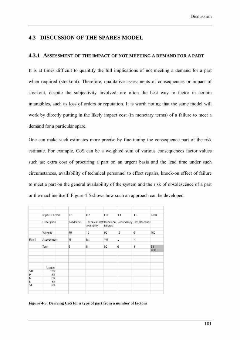
Discussion
101
4.3 DISCUSSION OF THE SPARES MODEL
4.3.1 ASSESSMENT OF THE IMPACT OF NOT MEETING A DEMAND FOR A PART
It is at times difficult to quantify the full implications of not meeting a demand for a part
when required (stockout). Therefore, qualitative assessments of consequences or impact of
stockout, despite the subjectivity involved, are often the best way to factor in certain
intangibles, such as loss of orders or reputation. It is worth noting that the same model will
work by directly putting in the likely impact cost (in monetary terms) of a failure to meet a
demand for a particular spare.
One can make such estimates more precise by fine-tuning the consequence part of the risk
estimate. For example, CoS can be a weighted sum of various consequences factor values
such as: extra cost of procuring a part on an urgent basis and the lead time under such
circumstances, availability of technical personnel to effect repairs, knock-on effect of failure
to meet a part on the general availability of the system and the risk of obsolescence of a part
or the machine itself. Figure 4-5 shows how such an approach can be developed.
Figure 4-5: Deriving CoS for a type of part from a number of factors

Risk Based Life Management of Offshore Structures and Equipment
102
The approach consists of the following main steps:
(1) Identify factors (termed as Impact Factors (IF) in figure 4-5) that impinge on failure to
meet a demand for a type of spare. In the figure, these are lead time, availability of technical
staff, knock-on failures and associated demands, potential for machine or spare redundancy
and obsolescence
(2) Ascribe weights to each of these impact factors to reflect their relative importance. These
are 10, 10, 60, 15, and 5 for IF1 through to IF5 respectively.
3) Determine relative importance values for VH, H, M, L or VL representing Very High,
High, Medium, Low and Very Low. In the approach shown in the figure, these are 100, 80,
60, 40 and 20 respectively.
(4) The spare type is then assessed qualitatively- VH, H, M, L or VL - under each of the
impact factors identified in step (1). The net result of this exercise is a total Impact Value or
the CoS for the type of part under consideration.
In the figure, the value ‘8’ in the first column is (10*80)/100. Weights need to total 100 as this
is a relative assessment; the weighted total ‘84’ is the CoS value for that part. This process is
repeated for each type of spare part that is under consideration in an inventory. The relative
weights or values in step (2) and step (3) may or may not be the same for all parts. Indeed,
impact factors also may differ with parts.
4.3.2 THE STARTING ASSUMPTION REGARDING ‘IDEAL’ STOCK LEVEL TO MEET
A MAXIMUM DEMAND LEVEL
The starting assumption is necessary to set a baseline. A distinction must be noted: ‘ideal’
values here mean the hypothetical scenario in which the decision maker has no constraints;
this is in contrast to optimal values or optimised values that are values that represent optimum
Discussion
103
trade-offs, given the constraints that apply. The starting assumption is more in the nature of a
carefully thought of scenario considering historical data, expert opinion or guesstimates.
For example, if one has no incidence of a propeller failing in a particular fleet of ships, one
might consider a bigger sample or use expert engineering judgement to assess demand. If one
was charged with the responsibility of stocking grit for next year’s winter, one reasonable way
to start assessing the demand would be to look at what has been the maximum demand in the
past, say, five years and use this as a benchmark.
4.3.3 CHANGES TO THE RATE OF DEMAND
In the calculations carried out, this model uses a demand trend for each type of part in the
period under consideration. The trend is considered fixed in this snapshot in time. The model
in its current form is thus based on periodic reviews of the stockholding using prior
experience.
The assessment of the demand can be made continuous by using a moving average method for
the demand trend. This would represent a continuous review model that may be more
advantageous in some circumstances. The model can also be configured to take in statistical
distributions other than the discrete uniform distribution in describing the demand for parts.
The rate of demand for parts may well increase as structures or equipment get older. This
change in the rate of demand is another factor that could be built into a spares inventory
model. It would require a more sophisticated treatment of time dependent effects that is
beyond the scope of this work.

Risk Based Life Management of Offshore Structures and Equipment
104
4.4 CONCLUSIONS
Research described here applies risk based principles to spares inventory management within
the context of life management of offshore structures and equipment. It extends the risk based
approach that is well established in other areas of industry. The example illustrates a
technique of managing risk within user specified constraints as applicable to spares inventory.
The approach outlined here has the potential to increase plant or system availability and
manage business as well as operational risks. It is thus of wider interest to a number of other
stakeholders including operators, maintenance personnel, regulators and insurance companies,
and other industries. The methodology can also be used in other areas that impinge on
structural integrity and asset management such as inspection and maintenance where
competing risks (of failure) need to be managed within finite resources

Discussion
105
5 DISCUSSION
5.1 APPLICATION OF RISK BASED APPROACHES
Risk based approaches offer a flexible, efficient and rational basis to life management of
assets. The previous chapters discussed methodologies that used risk based criteria for
decision making in the management of assets. The methodologies were applied in two
different contexts: (1) in the undertaking of run-repair-replace decision-making in the
management of offshore wind farms, and (2) in the optimal stocking of spares to cater for
failures requiring these. Some of the features of the applications of the risk based approaches
that stand out are as follows:
(a) The use of risk based optimisation
Risk based optimisation considers three aspects of failures: the likelihood, the
consequence and the manageability of failures within the resources available. In the first
application in the management of offshore wind farms, the approach shown aims at
finding the optimum time of action (repair or replacement), given a budget, such that the
cost of such action is less than or equal to the expected cost of failure without that action.
In the second application, risk based optimisation is used to find the optimum number of
spares of different kinds a company should advance order such that the cost of holding
these spares and the expected cost (risk) of not holding these are within user specified
limits.
Risk based optimisation thus takes risk assessment to a more advanced level: from
assessing risk to managing risk within the constraints that apply.

Risk Based Life Management of Offshore Structures and Equipment
106
(b) Quantitative and qualitative risk models
In both of the above applications, qualitative risk models have been used. In the first
application, as a screening tool in order to focus attention on components that are
perceived as more at the risk of failure, and in the second, to risk-profile spares such that
those that are deemed to have a bigger impact are accorded higher priority in stocking
them in an inventory.
Qualitative risk models give a good system-wide perspective and usually involve plant
personnel and experts. The screening out of low risk components and the flagging up of
high risk component is useful: the identified high risk components can then be analysed
using more advanced quantitative methods that usually require more resources. At times,
for want of quantitative data, qualitative models are the only option available to risk
assessors.
In the application to spares inventory management, a semi-quantitative model using
relative risk measures is used. This is to get over the difficulty of quantifying certain
factors such as the risk of obsolescence of a spare part. The concept of relative risk helps
in profiling the parts using a common denominator for risk.
In engineering there is a justifiable bias towards measuring and quantifying entities. The
American Petroleum Institute’s Recommended Practice 580 on risk-based inspection
describes a ‘continuum of approaches’ ranging from the qualitative to quantitative, figure
5-1. The figure depicts the level of detail in risk analysis corresponding to a purely
qualitative approach on one end of the spectrum, to the purely quantitative one on the
other, with intermediate approaches in between. Quantitative models do contain a higher
level of details, but the accuracy of the model depends on the availability and the quality of
the inputs. Thus in some situations the use of qualitative or intermediate type of models is
warranted. The ultimate test of any model is how closely it depicts reality.
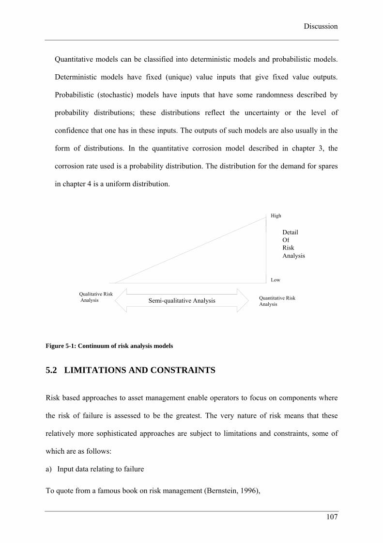
Discussion
107
Quantitative models can be classified into deterministic models and probabilistic models.
Deterministic models have fixed (unique) value inputs that give fixed value outputs.
Probabilistic (stochastic) models have inputs that have some randomness described by
probability distributions; these distributions reflect the uncertainty or the level of
confidence that one has in these inputs. The outputs of such models are also usually in the
form of distributions. In the quantitative corrosion model described in chapter 3, the
corrosion rate used is a probability distribution. The distribution for the demand for spares
in chapter 4 is a uniform distribution.
Figure 5-1: Continuum of risk analysis models
5.2 LIMITATIONS AND CONSTRAINTS
Risk based approaches to asset management enable operators to focus on components where
the risk of failure is assessed to be the greatest. The very nature of risk means that these
relatively more sophisticated approaches are subject to limitations and constraints, some of
which are as follows:
a) Input data relating to failure
To quote from a famous book on risk management (Bernstein, 1996),
Qualitative Risk Analysis
Quantitative Risk Analysis
Semi-qualitative Analysis
High
Low
Detail Of Risk Analysis

Risk Based Life Management of Offshore Structures and Equipment
108
“The information that you have is not the information you want.
The information you want is not the information you need.
The information you need is not the information you can obtain.
The information you can obtain costs more than you want to pay.”
In risk based approaches to life management, such as in the management of offshore wind
farms and spares inventory, it is assumed that relevant data regarding the mechanisms or
observed frequency of failures is available and applicable to the equipment being considered.
In practice, a lack of availability and applicability of failure data limits the efficacy of risk
based approaches. Sometimes data is not in a suitable format. At times, the failure dataset
(sample size) is too small for assessors to extract reliable statistical parameters.
Generic failure databases, (usually from the original equipment manufacturer (OEM) or
through generic databases such as, WindStats for onshore wind farms, or the GADS
(Generating Availability Data System) from NERC (North American Electric Reliability
Corporation) for power generating units), correspond to equipment operated under a range of
industry conditions. Sources of information such as logbooks that provide information
relating to specific equipment operating under specified conditions, and therefore containing
potentially more relevant and applicable data, are often not available. There is an inherent
problem in applying generic failure databases to make predictions for specific equipment
because the variability of design and operating conditions within the population as a whole
may not be representative.
In order to determine the probability of failure from damage mechanisms (e.g. fatigue,
corrosion, fracture, collapse, and extreme loads), distributions of the stochastic variables of
material properties, loads etc are required. In order to obtain representative distributions, a
large amount of experience and/ or experiments relevant to the application may be needed.
Discussion
109
These entail the use of substantial resources, and, in practice, the confidence that may be held
in such distributions may be questionable.
b) Understanding of the degradation and failure processes
Risk based approaches in the management of structures and equipment are limited by the
current understanding of the degradation and failure processes. Although much advance has
been made in understanding damage mechanisms such as fatigue, creep and corrosion, more
research continues in these and other areas. There are on-going challenges to understand the
effect of the operating environment, such as variable amplitude loading on fatigue, the
kinetics of different corrosive media (e.g. sour products), and the creep in new alloys and
welds.
c) Uncertainty in assessing failure consequences
Apart from the difficulty in assessing the likelihood of failure, the consequences of failure are
also at times difficult to ascertain. In some cases, the postulated failure event has never
occurred or is a very low probability event and there is therefore no or little prior experience
to use. How should one treat extremely low probability but potentially high consequence
events? One possible way is to design to fail-safe criteria such that failure does not result in
the high consequence under consideration. Low probability- high consequence events are
discussed in 5.3, under (c).
Other uncertainties may arise for the following reasons:
i) The impact of failure in complex systems with a number of interactions and
correlations is difficult to assess. There may be multiple consequences such as loss of

Risk Based Life Management of Offshore Structures and Equipment
110
property, life/injury, environmental damage, clean-up costs, production loss,
reputational damage, legal costs and so on.
ii) In systems operating in multiple- jurisdictions where different Class, regulations or
laws apply, the consequences of a potential failure may be difficult to assess or open
to more than one interpretation. As examples, litigation relating to the 1984 Bhopal
gas tragedy in India is still ongoing; nuclear accidents and oil spills may involve a
number of countries.
iii) Assessing the consequences of potential failures resulting in the loss of lives is a
complex matter. Although insurance companies have methods to quantify such events
in financial terms, intangibles such as loss of reputation, loss of morale among
employees may be difficult to measure.
d) Requirement for specialist and trained personnel
Engineering analyses, such as numerical modelling, that are often used to determine the
probability and consequences of a failure event, usually requires specialist knowledge, skills
and computing power. Personnel involved in day-to-day functioning of equipment do not
usually have the expertise to conduct such engineering analyses; it may require trained people
dedicated to this task in-house and/or expensive consultancy.
e) Technical complexity
Risk analyses can become very complex in a system with many components with
interdependencies and correlations in factors affecting failure and its consequences. Often it is
necessary to make simplifying or bounding assumptions. It may not be possible to analyse the
whole range of failure events each with its set of consequences. Risk models, like other
Discussion
111
models, are simplifications of reality; the predictions are subject to potential error. A
combination of variables, each having some error, may result in considerable error.
f) Subjectivity in qualitative assessments
Qualitative risk assessments tend to be subjective. To ensure, as far as possible, consistent
results, a suitable methodology that is auditable needs to be put in place. Formal processes to
elicit expert opinion can reduce the impact of biases that may colour an expert’s outlook.
g) Reliability of inspection and NDT techniques and application
Non-Destructive testing and Condition Monitoring provide vital inputs to the life
management of structures and equipment but have their own limitations. Human factors, the
probability of detection, the feasibility of sample size are some of the issues involved in
inspection and NDT techniques. Condition Monitoring is not considered economical in some
situations and the knowledge of the condition of a structure or equipment may not be good or
up-to-date.
h) Predicting risk
Risk models identify potential risks and predict failures and their consequences based on
some assumptions. It is important to note that these are predictions (expectations or expected
values) involving probability and need to be treated as such. At times, events may not occur
as predicted. There is a danger of this leading to a general disillusionment with such
techniques.
Risk Based Life Management of Offshore Structures and Equipment
112
i) Societal awareness of risk
The risk based approaches described here should not be treated in isolation: they need to be a
part of a wider culture of risk awareness informing people, processes and technology
involved. There is a need to incorporate other perspectives apart from those that result from
pure science and engineering analyses. In this context, human factors i.e. the role of humans
in failures is a matter of ongoing research. There is also increasing interest in the role of
organisation and its structure in managing risks.
j) Managing risks optimally, not just cutting costs
The philosophy behind risk based approaches is to optimise resources in the management of
risks; the aim is to focus resources on components identified as having high risk of failure.
Although a successful risk based approach will reduce failures and hence the costs resulting
from failures, it is not and should not only be construed as a part of cost cutting exercise in the
management of assets.
k) Upfront costs in managing risks
Reducing the level of risk often entails upfront costs that can be justified only in the long run;
risk mitigation thus needs foresight and the ability to invest in a safer future even if this
means foregoing immediate gains. Some companies are not prepared to make the investment
in risk based approaches.
l) Recognition of risk management professionals within business
Risk management professionals become the focus of attention particularly when bad things
happen or when risk management systems fail. They need to be taken seriously even during

Discussion
113
normal times and, indeed, be rewarded for continued safe operations. Some companies do not
sufficiently value their risk management professionals.
5.3 FURTHER DEVELOPMENTS
Research undertaken for this thesis shows that notwithstanding the limitations and constraints
identified above, there is scope for further development within the field of risk based life
management of structures and equipment. Some of the areas for development are described
below:
(a) Improving the quality (precision) of input data to risk assessment.
Recent advances in equipment monitoring and better ICT (Information and Communication
Technologies) are improving the quality of failure data that is being available for life
management of structures and equipment. Operators increasingly find it in their interest to
share failure data and there are a number of failure databases being set up to achieve this. The
RISPECT (Risk Based Expert System for Through-Life Structural Inspection, Maintenance
and New-Build Structural Design) project is an example of a number of stakeholders in the
shipping industry coming together to share inspection and failure data. RISPECT involves the
setting up of a hierarchy of databases (mainly comprising ship managers’ databases,
classification bodies’ databases and a central statistical database) containing relevant shipping
data and a number of modules that perform risk and reliability calculations using this data
(The website http://www.rispect.org.uk/ contains more information). Other databases
containing failure data such as WindStats and NERC-GADS are the result of collaboration
between various stakeholders in the relevant industry sector.

Risk Based Life Management of Offshore Structures and Equipment
114
(b) Greater understanding of degradation mechanisms
With increasing experience and research, there is a trend of having a greater understanding of
the degradation mechanisms involved in the ageing of assets. For example, understanding of
fatigue requires experimental data. Faster computers have made it easier to make complex
calculations and build complex models to link experiment to reality. The variability in the
action of degradation mechanisms and the correlations between them are increasingly being
calculated.
(c) More attention on towards low probability- high consequence events
There is increasing interest in low probability and high consequence events. Such events are
difficult to manage as: a) these are by definition extreme events, hence experience of dealing
with them is not always sufficient to draw lessons from and build a model on, and b) these
events are often so rare that measures to prevent/ mitigate such individual unlikely events are
not deemed cost-effective.
Concerted action to deal with extreme events that have common severe consequences is often
seen as a feasible way to prepare for such events. Industries have formed special networks to
pool resources to prepare for such rare adversities. For example, a group made up of the ICE
(Institution of Civil Engineers), the Royal Institute of British Architects, the Royal Institute of
Chartered Surveyors, the Royal Town Planning Institute and the Landscape Institute, works
together to manage and mitigate floods. The Fire and Blast Information Group (FABIG) is the
result of offshore industry collaboration, following the Piper Alpha disaster, to collate and
disseminate existing knowledge on hydrocarbon fires and explosions.

Discussion
115
Governments too form special committees that include representatives from law enforcement
bodies, the medical fraternity and others to respond to crises that are rare but require these
common resources.
Should every low probability- high consequence event be protected against? A balance is
required between risk mitigation and acceptable consequences. Typically, a risk assessment is
required to identify mitigation and acceptable costs. Some extremely low probability events
may remain unforeseen and therefore not a part of any risk assessment model; the best
approach in such circumstances is often to focus on responding to the new situation such that
the impact of such event in minimized.
(d) New applications of risk based methods
Risk based methods are being used in a variety of areas in industry. For example, there is
interest in using such risk based techniques to optimise inspection and maintenance in ships
and FPSO vessels.
(e) The need for a holistic approach to risk management
There is increasing interest in taking a holistic view in managing risks. This includes better
integration and coordination between people, processes and technology. This is done through,
as examples, better training, policy-making and guidelines in handling interfaces within and
between systems.
(f) Stakeholders in risk management

Risk Based Life Management of Offshore Structures and Equipment
116
Risk based approaches are, in large part, driven by the operators’ desire to allocate resources
in a flexible, rational and an efficient way. However, their application is also influenced by
legal and social forces. The role of regulation in the use of risk based approaches is gaining
prominence. Public awareness regarding risk and its management in industry has never been
higher.

Concluding Remarks
117
6 CONCLUDING REMARKS
The following sums up the main points from the research undertaken within the remit of this
Doctor of Engineering thesis
1. Research presented here describes new applications of risk based approaches to two
specific decision making situations involving the life management of structures and
equipment:
(a) Given a failure trend, when is the optimum time of action (repair/ replace a
structure or equipment) such that the net cost of the action and the expected cost
(risk) of failure is minimised and hence financial efficiency optimised? The
particular application was maintenance optimisation in the life management of
offshore wind farms.
(b) How many parts of different kinds, with each having its own associated
stocking costs and stockout risks, should a major industrial enterprise advance
order for stock to operate at optimum efficiency given that failures (requiring
these) may occur in service? The particular application was a fleet of cargo ships
where parts of different kinds are required to keep ships available for service.
2. The optimisation techniques in risk management described in this thesis find the
optimum trade-off between the cost of a risk mitigating measure and the expected cost
(risk) of failure without that measure. They have the potential of being applied more
widely within structural integrity and asset management, and indeed in any situation
where competing risks need to be managed within finite resources. They may
therefore find application in areas such as risk based inspection and maintenance, and
more generally, in other areas of risk management in engineering.

Risk Based Life Management of Offshore Structures and Equipment
118
3. The nature of risk poses a number of challenges to its assessors. Uncertainty in input
data is likely to remain a limitation. The question then is how this uncertainty in data
is accounted for in a risk assessment. The bottom-line in any assessment of risk is the
application of scientific method to the maximum extent possible and the continual
testing of prediction against empirical data.
4. The application of risk based approaches to life management of assets is a relatively
recent development. It is expected that in an increasingly competitive environment the
uptake of these approaches will become more prevalent in industry. This is because
risk based approaches offer rational, efficient and somewhat flexible ways of
maintaining assets.

References
119
7 REFERENCES
Anderson, C. 2006, The Long Tail- Why the future of business is selling less of more, 1st edn,
Hyperion, USA.
Andrews, J.D. & Moss, T.R. 2002, "An Introduction to Reliability and Risk Assessment" in
Reliability and Risk Assessment, Second edn, Professional Engineering Publishing, UK,
pp. 9.
API 2002a, Risk-based Inspection, API Recommended Practice 580, American Petroleum
Institute, USA.
API 2002b, Risk-based Inspection, API Recommended Practice 580, American Petroleum
Institute, USA.
API , API Risk Based Inspection Software [Homepage of Americal Petroleum Institute],
[Online]. Available: http://www.api.org/Publications/rbi-software.cfm [2009, October/8]
API Publication 2000, "Risk-Based Inspection, Base Resource Document" in , pp. 5-1-5-4.
ASME 2003a, "10. Multiple component ranking based upon optimization" in Risk-based
methods for equipment life management, CRTD Vol.41 ASMW, New York, pp. 151-152.
ASME 2003b, Risk Based Methods for Equipment Life Management: A Step-by-Step
Instruction Manual with Sample Applications, .
ASME International 2003a, "Introduction: Risk Based Methods for Equipment Life
Management" in Risk Based Methods for Equipment Life Management, CRTD Vol 41
ASMW, New York, pp. 3-4.
ASME International 2003b, "Risk Based Methods for Equipment Life Management, CRTD
Vol 41" in ASMW, New York, pp. 3-4.

Risk Based Life Management of Offshore Structures and Equipment
120
Ayyub, Bilal M. (2001) Elicitation of Expert Opinion for Uncertainty and Risks, Washington:
CRC Press.
Ayyub, Bilal M. (2003) Risk Analysis in Engineering and Economics, Washington: CRC
Press
Bernstein, Peter L. 1996, Against the Gods- The remarkable story of risk, John Wiley & Sons
Inc, USA, pp.202.
Brealey, R.A. & Myers, S.C. 1991, Principles of Corporate Finance, 4th edn, McGraw-Hill,
New York.
BSI 2008, PAS 55-1:2008 Asset Management- Part 1: Specification for the optimized
management of physical assets, BSI, UK.
Bureau Veritas , Asset Integrity Management. Available:
http://www.bureauveritas.co.uk/wps/wcm/connect/bv_couk/Local/Home/bv_com_service
SheetDetails?serviceSheetID=2153&siteID=3&industryID=-
1&serviceCategoryID=1&preciseObjectID=-1&divisionID=-1&businessScopeID=-1
[2009, September/9] .
Burton, Tony; Sharpe, David; Jenkins, Nick and Bossanyi, Ervin. 2001, Wind Energy
Handbook, pp.1-8
Caithness wind farm information forum, date unknown,
http://www.caithnesswindfarms.co.uk/
CIRIA 2009, Whole-life infrastructure asset management: Good practice guide for civil
infrastructure, CIRIA, London.
Clemen, R.T. & Winkler, R.L. 1999, "Combining Probability Distributions From Experts in
Risk Analysis", Risk Analysis, vol. 19.

References
121
Collier, A.C. & Glagola, R.C. 1998, "Chapter 16 Depreciation" in Engineering Economic and
Cost Analysis, 3rd edn, Addison-Wesley, California, USA, pp. 439.
Department of Trade and Industry. Future Offshore: A strategic framework for the Offshore
Wind Industry, 2002
Det Norske Veritas June 2004, Offshore Standard DNV-OS-J101; Design of Offshore Wind
Turbine Structures, DNV, Norway.
DOWEC; http://www.ecn.nl/docs/dowec/10048_004.pdf
EEMUA 2006, Risk Based Inspection- A guide to effective use of the RBI process, EEMUA,
UK.
ISO/ IEC Guide 51:1999 1999, ISO/IEC Guide 51:1999 Safety aspects- Guidelines for their
inclusion in standards, ISO/IEC.
Kennedy, W.J., Wayne Patterson, J. & Fredendall, L.D. 2002, "An overview of recent
literature on spare parts inventories", International Journal of Production Economics,
vol. 76, no. 2, pp. 201-215.
Lee, A.K., Serratella, G., Wang, G., Basu, R. & Spong, R. 2006, "Flexible Approaches to
Risk-Based Inspection of FPSOs", Offshore Technology ConferenceU.S.A.
Manwell, J. F., McGowan, J. G. and Rogers, A. L. Introduction: Modern Wind Energy and its
Origins 2005
Nahmias, S. 1981, "Managing Reparable Item Inventory Systems: A Review", TIMS Studies
in the Management Sciences, vol. 16, pp. 253-277.
O’Hagan, Anthony; Buck, Caitlin E., Daneshkhan, Alireza; Eiser, J; Garthwaite, Paul H.;
Jenkison, David J., Oakley, Jeremy E.; Bakow, Tim. (2006) Uncertain Judgements:
Eliciting Experts’ Probabilities (Statistics in Practice), UK, John Wiley & Sons Ltd

Risk Based Life Management of Offshore Structures and Equipment
122
PD ISO/IEC Guide 73:2002 2002, Risk Management- Vocabulary- Guidelines for use in
standards, BSI British Standards.
Prasad, S. 1993, "Classification of inventory models and systems", International Journal of
Production Economics, vol. 34, pp. 209-222.
Putnam, G. C. Power from the wind 1948
RISPECT home page, Available: http://www.rispect.org.uk/ [2009, November/ 21] .
Rumsfeld, D. 12 February 2002, Former US Defence Secretary on the situation in Afganistan
then.
Taleb, N.N. 2007, The Black Swan, Penguin Books, UK.
Vose, D. 2008, "Choice of Model Structure" in Risk Analysis, Third edn, John Wiley & Sons,
Ltd, UK.
Winston, L.W. 1993, Operations Research- Applications and Algorithms, Third edn, Duxbury
Press, California, USA.
Wintle, J., Moore, P., Smalley, S. & Amphlett, G. 2006, "Section 3 Identification of Ageing"
in Plant ageing: Management of equipment containing hazardous fluids or pressure
HSE, UK, pp. 43.
(The) Woodhouse Partnership Ltd, 2008, ‘Education and Training in Asset Management’,
www.twpl.com.
Zomerdijk, L.G. & de Vries, J. 2003, "An organizational perspective on inventory control:
Theory and a case study", International Journal of Production Economics, vol. 81-82, pp.
173-183.

Appendix A: Paper 1
123
APPENDIX A : PAPER 1
Bharadwaj, U.R., Speck, J.B. & Ablitt, C.J. 2007, "A practical approach to risk based
assessment and maintenance optimisation of offshore wind farms", Offshore Mechanics and
Arctic Engineering (OMAE), ASME, June 10-15, 2007, San Diego, California, USA.

Risk Based Life Management of Offshore Structures and Equipment
1 Copyright © ASME 2007
Proceedings of OMAE2007
26th International Conference on Offshore Mechanics and Arctic Engineering
June 10-15, 2007, San Diego, California USA
OMAE 2007-29260
A PRACTICAL APPROACH TO RISK BASED ASSESSMENT AND MAINTENANCE
OPTIMISATION OF OFFSHORE WIND FARMS
Ujjwal R Bharadwaj Loughborough University
Julian B Speck TWI Ltd, Cambridge
Chris J Ablitt TWI Ltd, Cambridge
ABSTRACT
Offshore wind farm managers are under
increasing pressure to minimise life cycle costs
whilst maintaining reliability or availability targets,
and to operate within safety regulation. This paper
presents a risk based decision-making methodology
for undertaking run-repair-replace decisions with the
ultimate aim of maximising the Net Present Value
(NPV) of the investment in maintenance. The paper
presents the methodology developed for the risk
based life management of Offshore Wind farms
under the remit of the CORLEX (Cost Reduction
and Life Extension of Offshore Wind Farms) project
funded by DTI (Department of Trade and Industry,
UK) Technology Programme on Renewable Energy.
Unlike traditional approaches to decision-making
that consider either the probability of failure of a
component or the consequence of failure in isolation,
a risk-based approach considers both these aspects in
combination to arrive at an optimal solution. The
paper builds a basic Qualitative Risk Analysis
methodology to highlight high-risk components that

2 Copyright © ASME 2007
are then investigated further by a Quantitative Risk
Analysis. The risk is now quantified in monetary
terms and the time of action – replacement or
maintenance- indicated by the model is such that the
NPV of the action is maximized. The methodology is
demonstrated by considering offshore wind turbine
tower as the critical component and corrosion as the
damage mechanism.
Keywords: Offshore wind farms, Maintenance, Risk
Based Decision Making, Quantitative Risk Analysis.
1 INTRODUCTION
Maintenance manages the process of ageing of a
plant or machinery. Ageing is a process that is
relentless and starts from the moment a product is
manufactured or fabricated. The rate of failure
versus time relationship is usually depicted by
Figure 1. During the initial stage- the Infant
Mortality stage, there are ‘teething’ problems
causing the failure rate to be high. The rate than falls
as these problems – design, manufacturing defects,
etc are identified and solved. In the second stage,
which is the Useful Life stage, standard maintenance
practices keep the failure rate almost constant.
During the third and final stage of the plant- the
Ageing stage, the failure rate rises mainly due to
damage accumulated by ageing. At some point
during this stage, high failure rate requires operators
to consider replacing the plant. In practice, there are
usually a number of such plants and a limited budget
available to decision makers.
This paper develops and demonstrates a risk-
based methodology to decide the optimum time of
replacement or repair of a plant, given, a number of
such plants, and limited budgetary support.
The paper starts with a discussion on risk and its
analyses- qualitative and quantitative, the concept of
NPV, and moves on to the trade off involved in risk-
based decision-making within budgetary and safety
constraints.
2 RISK
Risk has numerous definitions depending upon
its use. Risk is a combination of the probability of an
event and its consequence. (API 2002) It is a

3 Copyright © ASME 2007
deviation from the normal or expected. Numerically,
it is a product of probability of an event occurring
and the consequence of the event.
3 THE RISK BASED APPROACH TO
MAINTENANCE
A risk-based approach considers failure in both
its dimensions, taking cognizance of the two
elements that constitute risk- the probability (or
likelihood) of failure and the consequence of that
failure. Figure 2 shows the two dimensional risk
profiles of the components in an offshore wind
turbine plant henceforth referred to as the plant.
The probabilities and the consequences of failure
of ten components have been determined and
presented as points on a Risk Plot. An iso-risk line is
also plotted representing a constant risk level as
defined by the operator according to their perception
of what is an acceptable threshold level of risk. The
iso-risk line separates acceptable risk components
from the unacceptable risk components, enabling
plant managers to focus maintenance resources on
the relatively more risky components.
Risk analysis is the systematic use of information
to identify sources of risk, and to estimate the risk of
failure. It forms the basis for risk evaluation, risk
mitigation and risk acceptance (or risk avoidance).
The information used in risk analysis includes
historical data, theoretical analysis, informed
opinions and stakeholder concerns.
4 RISK ANALYSIS METHODS
Risk analysis methods are generally categorised
as qualitative or quantitative. There may be an
intermediate category (semi-quantitative) depending
upon how quantitative the risk analysis is. The
American Petroleum Institute’s Recommended
Practice 580 on risk-based inspection describes a
‘continuum of approaches’ ranging from the
qualitative to quantitative, Figure 3. The figure
depicts the level of detail in risk analysis
corresponding to a purely qualitative approach on
one end of the spectrum, to the purely quantitative
one on the other, with intermediate approaches in
between.
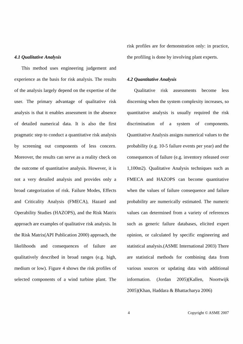
4 Copyright © ASME 2007
4.1 Qualitative Analysis
This method uses engineering judgement and
experience as the basis for risk analysis. The results
of the analysis largely depend on the expertise of the
user. The primary advantage of qualitative risk
analysis is that it enables assessment in the absence
of detailed numerical data. It is also the first
pragmatic step to conduct a quantitative risk analysis
by screening out components of less concern.
Moreover, the results can serve as a reality check on
the outcome of quantitative analysis. However, it is
not a very detailed analysis and provides only a
broad categorization of risk. Failure Modes, Effects
and Criticality Analysis (FMECA), Hazard and
Operability Studies (HAZOPS), and the Risk Matrix
approach are examples of qualitative risk analysis. In
the Risk Matrix(API Publication 2000) approach, the
likelihoods and consequences of failure are
qualitatively described in broad ranges (e.g. high,
medium or low). Figure 4 shows the risk profiles of
selected components of a wind turbine plant. The
risk profiles are for demonstration only: in practice,
the profiling is done by involving plant experts.
4.2 Quantitative Analysis
Qualitative risk assessments become less
discerning when the system complexity increases, so
quantitative analysis is usually required the risk
discrimination of a system of components.
Quantitative Analysis assigns numerical values to the
probability (e.g. 10-5 failure events per year) and the
consequences of failure (e.g. inventory released over
1,100m2). Qualitative Analysis techniques such as
FMECA and HAZOPS can become quantitative
when the values of failure consequence and failure
probability are numerically estimated. The numeric
values can determined from a variety of references
such as generic failure databases, elicited expert
opinion, or calculated by specific engineering and
statistical analysis.(ASME International 2003) There
are statistical methods for combining data from
various sources or updating data with additional
information. (Jordan 2005)(Kallen, Noortwijk
2005)(Khan, Haddara & Bhattacharya 2006)

5 Copyright © ASME 2007
In the current discussion, it is assumed that the
structure of a wind turbine tower is of critical
importance, as highlighted by the Qualitative
Analysis in the previous section.
For the Quantitative Risk Analysis method
proposed in this paper, a failure frequency versus
time curve, for the Ageing period of life is developed
by engineering analysis of the structure for the active
or potentially active in-service damage mechanisms,
e.g. corrosion. The consequence of failure is in
financial terms. For complex systems, event tree
analysis is usually undertaken to determine the effect
the particular component has on the system, to
thereby resolve the individual cost of consequence
of the component’s failure.
5. RISK BASED OPTIMISATION
The next step is the calculation of the optimum
action schedule or date, of the run-repair-replace
action. This calculation weighs the financial benefits
of maintenance action against the risk (as expressed
in costs) of not taking the action. The ultimate aim is
to maximise the net present value of the investment
(i.e. the maintenance action) by adjusting the date of
the action.
6.DECISION-MAKING USING FINANCIAL
CRITERION
6.1 The need for financial criterion in maintenance
decision making
Maintenance projects are increasingly being
evaluated by decision makers who need to
understand the implications of various options in
financial terms. Although predictive maintenance
techniques have matured, the predictions are in
engineering terms, and these are not easily
understood by financially oriented decision makers.
Thus, there is a need to express the effects of
engineering wear and tear in financial terms. In the
current context, this is done by evaluating the cost of
the consequences of failure owing to wear and tear
of plant and machinery.
6.2 The drivers for a consistent decision making
methodology in maintenance

6 Copyright © ASME 2007
Many old plants, structures, capital equipment or
components are in their Ageing period of life.
However, increasing competition means many of
them cannot be replaced and need to have their
useful life extended. In addition, new components
are often designed to operate with maximum
efficiency, and are designed with lower “margins of
error” against assumed operating conditions.
Each action (or project) has costs associated with
it. These costs are, in essence, investments made by
the concerned asset owner with the expectation of
certain return on the investment(s). The decision
maker will normally be faced with a number of
projects competing for such investments, and
therefore needs to take decisions that maximise the
returns on these investments. The most widely
understood financial techniques to evaluate projects
include ‘return on investment’, ‘pay-back period’
and ‘discounted cash flow (DCC)’ methods.(Brealey,
Myers 1991) These techniques have various
strengths and weaknesses. This paper employs the
net present value (NPV) technique that is a form of
DCC analysis.
7. Maximizing NPV using Probabilistic Damage
Mechanism Models
7.1 NPV Financial Analysis
In the current discussion, it is assumed that a
project with a higher NPV is a better investment than
a project with a lower NPV. The NPV of a project is
the present (current) value of the total future cash
flows, both positive (income) and negative (cost).
NPV considers the time value of money by
discounting all the cash flows, and it is calculated as
follows:
NPV =
N
t
tt rC
0
)1()( (1)
N = project life (years); t = timing of cash flow
(year); r = interest rate, or discount rate; and Ct =
cash flow in year t.

7 Copyright © ASME 2007
The future cash flows are ‘expected’ cash flows,
as they do not occur with certainty. The uncertainty
arises in the engineering analysis to calculate the
probability of failure over time for the damage
mechanism(s) of interest.
The risk associated with any project is finally
expressed in terms of its NPV by using expected
values (EV). The EV of a failure event is the product
of the probability of the event occurring and the cost
of consequence of that event.
The cost of consequence of a failure event is
directly assessed from a prior quantitative
consequence analysis, and it must be expressed in
financial terms.
Thus, the NPV of a project with uncertain
outcomes is the sum of the expected values of all
future discounted cash flows, as follows:
NPV =
N
t
ttt rCp
0
)1()( (2)
pt = the probability of the event occurring at time
t.
7.2 Probabilistic Damage Mechanism Model
This paper does not discuss the details of damage
models for use in probabilistic analysis. Instead it
illustrates a simple probabilistic damage mechanism
model for general corrosion of the tower structure.
Consider a structure subject to corrosion. Assuming
this to be the only damage mechanism causing
failure of the structure, the remaining life of the
structure can be calculated as:
RL = (Tc–MAT)� CR
(3)
RL = remaining life (years); Tc = current
thickness of the structure (mm); MAT = minimum
allowable thickness (mm); and CR = corrosion rate
(mm/year).
CR is derived from periodic in-service
measurements of metal loss resulting from corrosion.

8 Copyright © ASME 2007
Tc is known from the most recent thickness
measurements on the structure (or at the start of the
structure’s life, Tc can be assumed to be equal to the
original nominal thickness of the structure as
specified by the designer including tolerances,
corrosion allowance, etc). MAT is the absolute
minimum thickness calculated by the designer to
prevent failure by overload, collapse, etc as
appropriate.
The convention is to calculate RL in a
deterministic manner, whereby each independent
variable in Equation 3 is a specific value. This
assumes that these variables have no random or
probabilistic aspects but can be defined in a fixed
predictable fashion. In reality, there is considerable
uncertainty associated with these variables and each
can be defined by a statistical distribution of values.
In the method here, a statistical analysis tool (i.e.
Palisade’s @RISK for Microsoft Excel) is used to
describe all the independent variables
probabilistically, and RL is then calculated using
Monte Carlo Simulation (MCS) technique. In this
way, the calculated RL by MCS is actually a
distribution of values, so that the annual probability
of failure (the failure rate per year) over time can be
obtained. This probability versus times curve may
then be used to derive the EV, where the EV of a
failure event is the product of the probability of the
event occurring and the cost of consequence of that
event, at a specific point in time.
7.3 Risk-based Optimisation
The key inputs to the optimisation model are as
follows:
(a) The expected present value of the proposed
action (replacement or repair of the asset); (b) The
expected present value of inaction which is equal to
the expected present value of the production losses
avoided as the result of undertaking the proposed
action; (c) Any financial constraints, such as the
annual maintenance budget limit; and (d) Any non-
financial constraints, e.g. on failure rates due to
safety regulations.
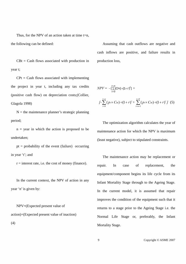
9 Copyright © ASME 2007
Thus, for the NPV of an action taken at time t=n,
the following can be defined:
CBt = Cash flows associated with production in
year t;
CPt = Cash flows associated with implementing
the project in year t, including any tax credits
(positive cash flow) on depreciation costs;(Collier,
Glagola 1998)
N = the maintenance planner’s strategic planning
period;
n = year in which the action is proposed to be
undertaken;
pt = probability of the event (failure) occurring
in year ‘t’; and
r = interest rate, i.e. the cost of money (finance).
In the current context, the NPV of action in any
year ‘n’ is given by:
NPV=(Expected present value of
action)+(Expected present value of inaction)
(4)
Assuming that cash outflows are negative and
cash inflows are positive, and failure results in
production loss,
NPV = ])1()([0
tnt
tPt rC
+
[- tnt
t
Btt rCp )1()(0
+ tNt
nt
Btt rCp )1()(1
] (5)
The optimization algorithm calculates the year of
maintenance action for which the NPV is maximum
(least negative), subject to stipulated constraints.
The maintenance action may be replacement or
repair. In case of replacement, the
equipment/component begins its life cycle from its
Infant Mortality Stage through to the Ageing Stage.
In the current model, it is assumed that repair
improves the condition of the equipment such that it
returns to a stage prior to the Ageing Stage i.e. the
Normal Life Stage or, preferably, the Infant
Mortality Stage.
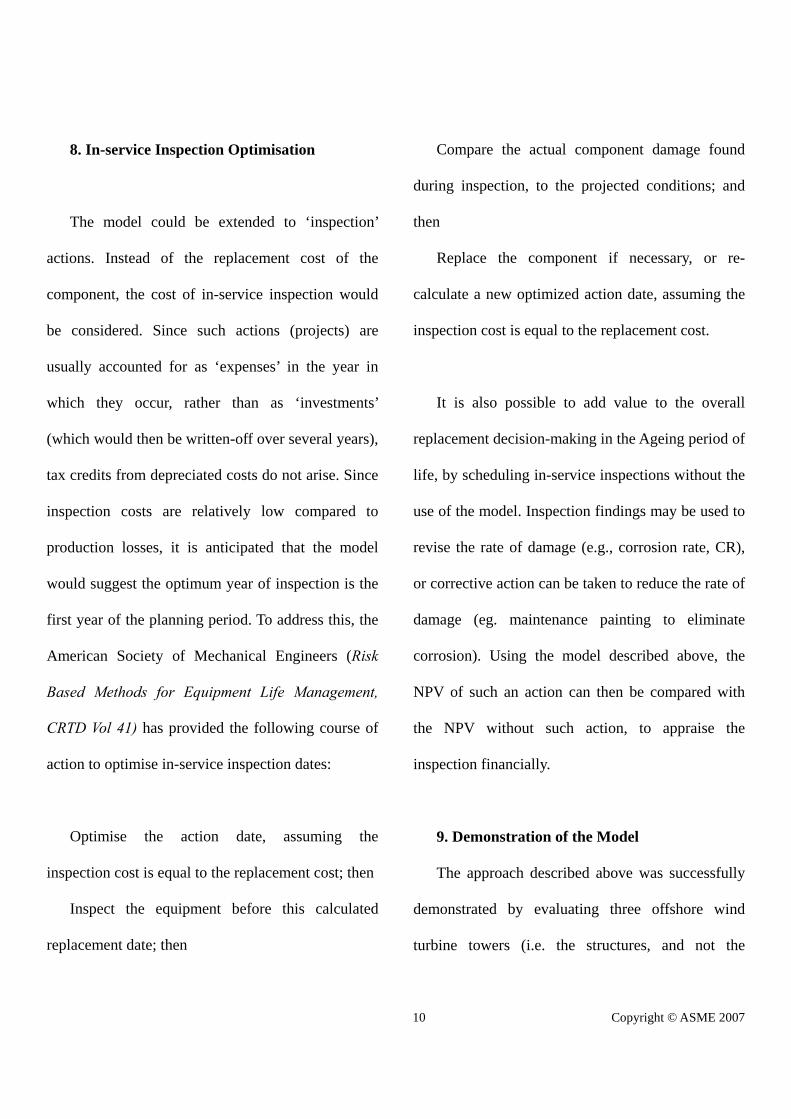
10 Copyright © ASME 2007
8. In-service Inspection Optimisation
The model could be extended to ‘inspection’
actions. Instead of the replacement cost of the
component, the cost of in-service inspection would
be considered. Since such actions (projects) are
usually accounted for as ‘expenses’ in the year in
which they occur, rather than as ‘investments’
(which would then be written-off over several years),
tax credits from depreciated costs do not arise. Since
inspection costs are relatively low compared to
production losses, it is anticipated that the model
would suggest the optimum year of inspection is the
first year of the planning period. To address this, the
American Society of Mechanical Engineers (Risk
Based Methods for Equipment Life Management,
CRTD Vol 41) has provided the following course of
action to optimise in-service inspection dates:
Optimise the action date, assuming the
inspection cost is equal to the replacement cost; then
Inspect the equipment before this calculated
replacement date; then
Compare the actual component damage found
during inspection, to the projected conditions; and
then
Replace the component if necessary, or re-
calculate a new optimized action date, assuming the
inspection cost is equal to the replacement cost.
It is also possible to add value to the overall
replacement decision-making in the Ageing period of
life, by scheduling in-service inspections without the
use of the model. Inspection findings may be used to
revise the rate of damage (e.g., corrosion rate, CR),
or corrective action can be taken to reduce the rate of
damage (eg. maintenance painting to eliminate
corrosion). Using the model described above, the
NPV of such an action can then be compared with
the NPV without such action, to appraise the
inspection financially.
9. Demonstration of the Model
The approach described above was successfully
demonstrated by evaluating three offshore wind
turbine towers (i.e. the structures, and not the
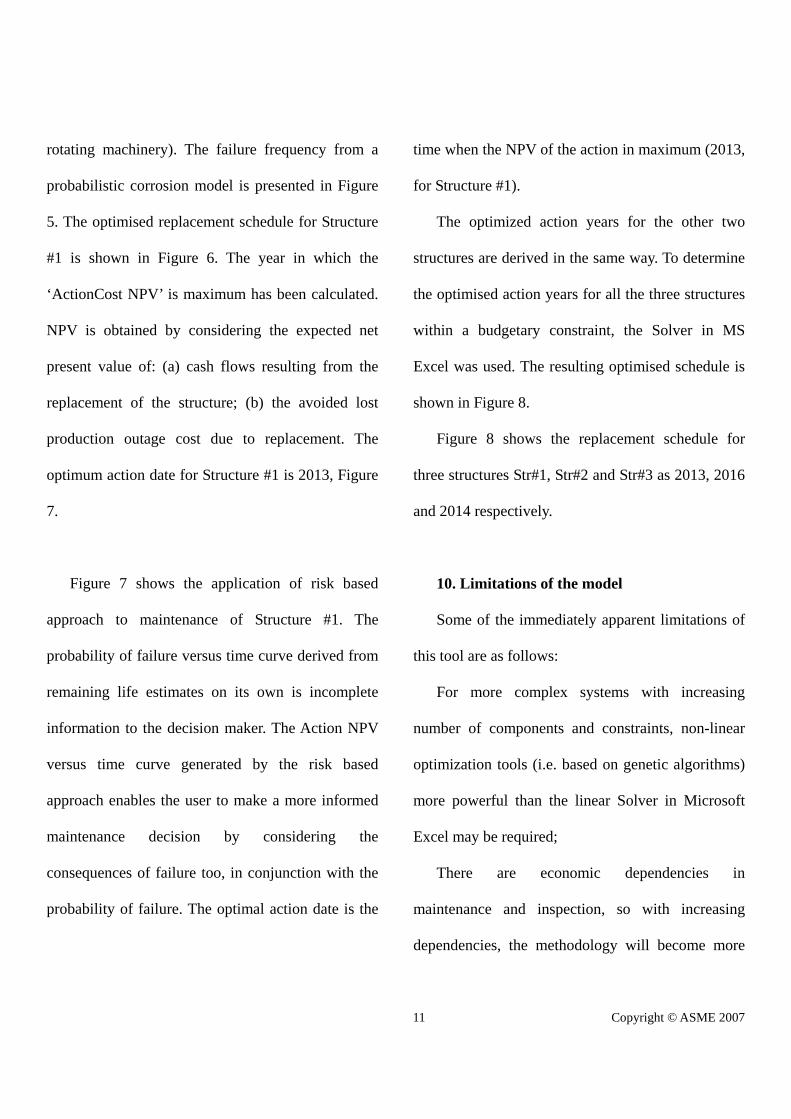
11 Copyright © ASME 2007
rotating machinery). The failure frequency from a
probabilistic corrosion model is presented in Figure
5. The optimised replacement schedule for Structure
#1 is shown in Figure 6. The year in which the
‘ActionCost NPV’ is maximum has been calculated.
NPV is obtained by considering the expected net
present value of: (a) cash flows resulting from the
replacement of the structure; (b) the avoided lost
production outage cost due to replacement. The
optimum action date for Structure #1 is 2013, Figure
7.
Figure 7 shows the application of risk based
approach to maintenance of Structure #1. The
probability of failure versus time curve derived from
remaining life estimates on its own is incomplete
information to the decision maker. The Action NPV
versus time curve generated by the risk based
approach enables the user to make a more informed
maintenance decision by considering the
consequences of failure too, in conjunction with the
probability of failure. The optimal action date is the
time when the NPV of the action in maximum (2013,
for Structure #1).
The optimized action years for the other two
structures are derived in the same way. To determine
the optimised action years for all the three structures
within a budgetary constraint, the Solver in MS
Excel was used. The resulting optimised schedule is
shown in Figure 8.
Figure 8 shows the replacement schedule for
three structures Str#1, Str#2 and Str#3 as 2013, 2016
and 2014 respectively.
10. Limitations of the model
Some of the immediately apparent limitations of
this tool are as follows:
For more complex systems with increasing
number of components and constraints, non-linear
optimization tools (i.e. based on genetic algorithms)
more powerful than the linear Solver in Microsoft
Excel may be required;
There are economic dependencies in
maintenance and inspection, so with increasing
dependencies, the methodology will become more
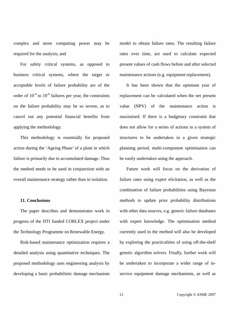
12 Copyright © ASME 2007
complex and more computing power may be
required for the analysis; and
For safety critical systems, as opposed to
business critical systems, where the target or
acceptable levels of failure probability are of the
order of 10-4 to 10-6 failures per year, the constraints
on the failure probability may be so severe, as to
cancel out any potential financial benefits from
applying the methodology.
This methodology is essentially for proposed
action during the ‘Ageing Phase’ of a plant in which
failure is primarily due to accumulated damage. Thus
the method needs to be used in conjunction with an
overall maintenance strategy rather than in isolation.
11. Conclusions
The paper describes and demonstrates work in
progress of the DTI funded CORLEX project under
the Technology Programme on Renewable Energy.
Risk-based maintenance optimization requires a
detailed analysis using quantitative techniques. The
proposed methodology uses engineering analysis by
developing a basic probabilistic damage mechanism
model to obtain failure rates. The resulting failure
rates over time, are used to calculate expected
present values of cash flows before and after selected
maintenance actions (e.g. equipment replacement).
It has been shown that the optimum year of
replacement can be calculated when the net present
value (NPV) of the maintenance action is
maximised. If there is a budgetary constraint that
does not allow for a series of actions in a system of
structures to be undertaken in a given strategic
planning period, multi-component optimisation can
be easily undertaken using the approach.
Future work will focus on the derivation of
failure rates using expert elicitation, as well as the
combination of failure probabilities using Bayesian
methods to update prior probability distributions
with other data sources, e.g. generic failure databases
with expert knowledge. The optimisation method
currently used in the method will also be developed
by exploring the practicalities of using off-the-shelf
genetic algorithm solvers. Finally, further work will
be undertaken to incorporate a wider range of in-
service equipment damage mechanisms, as well as

13 Copyright © ASME 2007
previous in-service inspection data, to optimise
future inspection plans (i.e. coverage and schedule).
12. Acknowledgements
The authors wish to acknowledge the support of
Professors Vadim Silberschmidt and John Andrews
at Loughborough University, and Mr John Wintle at
TWI.
References
API 2002, Risk-based Inspection, API Recommended
Practice 580, American Petroleum Institute,
USA.
API Publication 2000, "Risk-Based Inspection, Base
Resource Document" in, pp. 5-1-5-4.
ASME International 2003, Risk Based Methods for
Equipment Life Management, CRTD Vol 41,
ASME, New York.
Brealey, R.A. & Myers, S.C. 1991, Principles of
Corporate Finance, 4th edn, McGraw-Hill, New
York.
Collier, A.C. & Glagola, R.C. 1998, "Engineering
Economic and Cost Analysis" in , 3rd edn,
Addison-Wesley, California, pp. 438-464.
Jordan, I. 2005, Decisions under uncertainty:
Probabilistic Analysis for Engineering
Decisions,.
Kallen, M.J. & Noortwijk, J.M.V. 2005, "Optimal
Maintenance decisions under imperfect
inspection", Reliability Engineering & System
Safety,.
Khan, F.I., Haddara, M.M. & Bhattacharya, S.K.
2006, "Risk Based Integrity and Inspection
Modeling (RBIIM) of Process
Components/System", Risk Analysis, vol. 26, no.

14 Copyright © ASME 2007
ANNEX A
FIGURES
Figure 1: Failure rate of plant components versus age. 4 2 3 6 8 9 5 1 7 Iso-risk line 10 Consequence of failure
Figure 2: Idealised Risk Plot of several components within a plant.
Fai
lure
rat
e
Age in years
Infant mortality stage
Normal life with low almost constant
failure rate
Ageing stage with increasing failure
rate
P
roba
bili
ty o
f fa
ilur
e

15 Copyright © ASME 2007
Figure 3: Continuum of Risk Analysis methods.
Figure 4: Qualitative Risk Analysis using a Risk Matrix
Qualitative Risk Analysis Quantitative Risk
Analysis Semi-qualitative Analysis
High
Low
Detail Of Risk Analysis

16 Copyright © ASME 2007
Figure 5: Probability of failure versus time
Figure 6:Optimum time of replacement of Structure #1
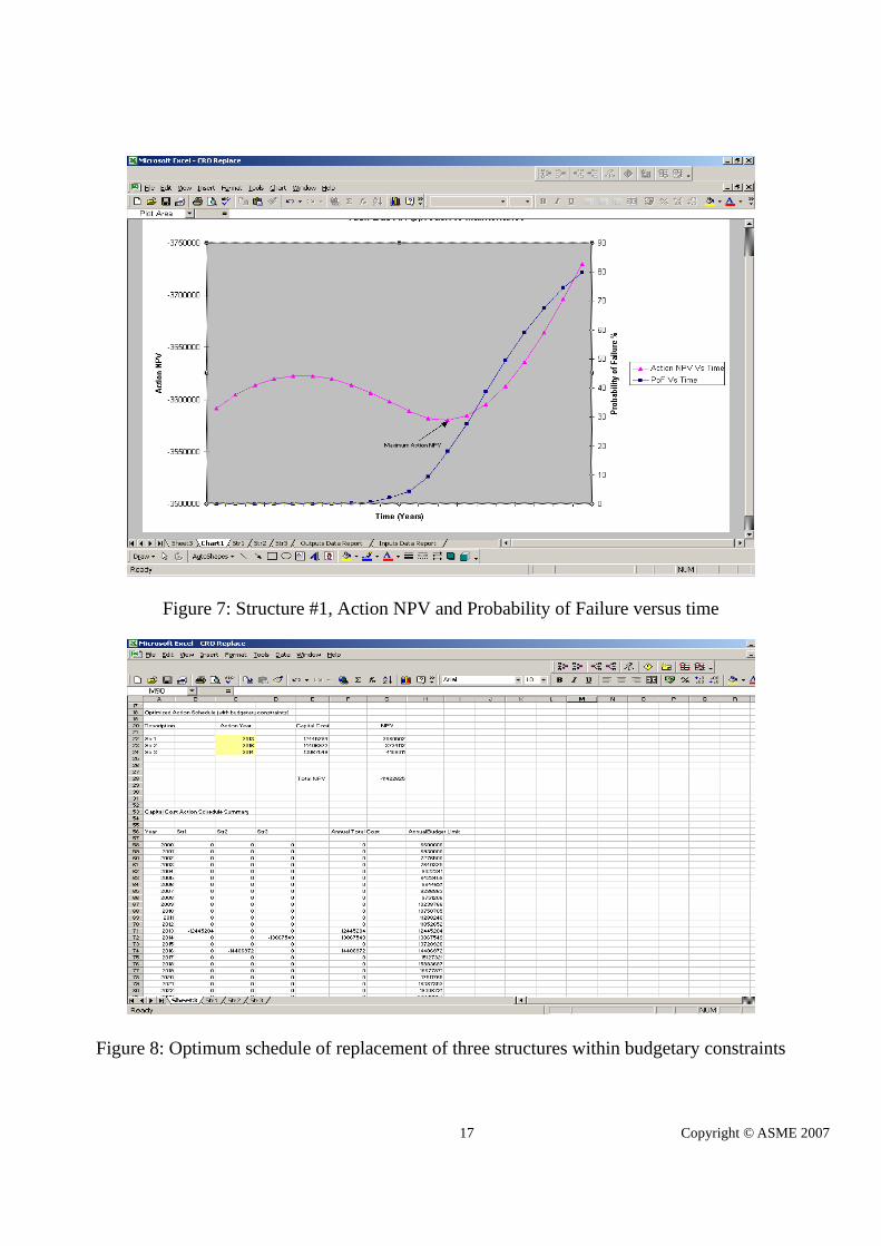
17 Copyright © ASME 2007
Figure 7: Structure #1, Action NPV and Probability of Failure versus time
Figure 8: Optimum schedule of replacement of three structures within budgetary constraints

18 Copyright © ASME 2007

Appendix B: Paper 2
APPENDIX B : PAPER 2
Bharadwaj, U.R., Silberschmidt, V.V., Wintle, J.B. & Speck, J.B. 2008, "A risk based
approach to spare parts inventory management", International Mechanical Engineering
Congress and Exposition (IMECE), ASME, November 2-6, 2008, Boston, Massachusetts.

Risk Based Life Management of Offshore Structures and Equipment
1 Copyright © 2008 TWI Ltd
Proceedings of IMECE2008 2008 ASME International Mechanical Engineering Congress and Exposition
November 2-6, 2008, Boston, Massachusetts, USA
IMECE2008-68845
A RISK BASED METHODOLOGY FOR SPARE PARTS INVENTORY OPTIMISATION
Ujjwal R Bharadwaj TWI Ltd, Cambridge, UK/
Loughborough University, UK
Vadim V Silberschmidt Wolfson School of Mechanical and
Manufacturing Engineering, Loughborough University, UK
John B Wintle
TWI Ltd Cambridge, UK
Julian B Speck Lloyd’s Register EMEA
London, UK
ABSTRACT
Spare parts inventories assist maintenance staff to keep equipment in operating condition.
Thus the inventory level of spares has a direct bearing on machine availability, a factor that is
increasingly important in capital-intensive industries. This paper presents a risk based approach
for spare parts inventory optimization.
At the outset, the paper highlights the unique features of maintenance inventories, such as
spare parts inventories, compared to other inventories such as work- in- progress or finished
product inventories. After a brief mention of the principles on which many of the current
inventory management models are based and their limitations, the paper presents a risk-based
methodology to spares inventory management. ‘Risk’ in the current context is the risk in

2 Copyright © 2008 TWI Ltd
monetary terms that arises when a component (spare) is not available on demand. It is the
expected value of loss, i.e., the product of the likelihood of unavailability of the spare from the
inventory and an estimate of the consequence(s) of that unavailability. Given a budgetary
constraint and the risk profile of a number of spares, the model gives an optimal inventory of
spares.
By basing the inventory on the risk profile of spares, the model includes factors that are not
normally considered in various other models. The ultimate aim of the methodology is to have an
optimal level of spares inventory such that machine availability, to the extent it is dependent on
the level of spares inventory, is maximized subject to constraints. The methodology is expected to
benefit both, operational and financial managers.
1.0 INTRODUCTION
The level of spares in an inventory has a direct bearing on machine availability. The
availability of a machine is a function of the mean time to correct a failure which in turn depends
upon, among other factors, the time to obtain a spare (to conduct repairs) or a replacement. The
level of spares in a spares inventory is constrained by the cost of holding stock and the penalty of
being out of stock. In a competitive climate companies strive to keep their spares inventory at an
optimum level to minimize the costs involved. This paper presents a new approach - a risk based
approach - to spares inventory management aimed at establishing an optimum level of spares
such that financial benefit is maximized within accepted levels of risk, and the remaining
(residual) risks are clearly identified. The paper presents a framework that enables consistent and
auditable decision making in spares inventory management.

3 Copyright © 2008 TWI Ltd
Risk based approaches are used in other sectors of industry and for prioritizing different
types of actions; for example, there are risk based approaches in the process industry to manage
maintenance and inspection and there are standards or guidance documents to implement these
approaches (1, 2, 3 and 4). As opposed to other approaches, in a risk based approach, actions are
based on the risk estimate of various options. In the current context, this means maintaining an
inventory at an optimal level depending on the risk profile of the spares in which the likelihood
of a failure to meet the demand for a spare is considered in conjunction with the consequences of
the failure to meet that demand. The optimal level is such that financial benefits are optimized
given risk associated constraints.
The paper discusses some of the unique features of spares inventories vis-à-vis other types of
inventories. There is also a section on typical costs associated with inventories followed by a
brief note on the main principles underlying various current approaches to spares inventory
management. The main body of the paper then presents the risk based methodology and the basic
model that has been created to implement that methodology. This is followed by limitations of
the methodology, areas of further research and conclusions.
2.0 SPARE PARTS INVENTORIES
Spare parts inventories are maintenance inventories; they are used by maintenance personnel
to keep machines available and exist to meet an internal demand for spares. They perform a
different function compared to other inventories such as Work-in-progress (WIP) inventories and
Finished Product Inventories. WIP inventories smooth out irregularities in production flow. These
irregularities are caused by factors such as changes in product mix, equipment breakdowns,
differences in production rates, between processes and material handling. Finished Product

4 Copyright © 2008 TWI Ltd
Inventories provide a buffer stock to protect against lead time demand, differences in quality
levels, differences in machine production rates, labor troubles, scheduling problems, gap between
capacity and demand and other well established production problems(5).
Characteristics of Spare parts inventories: Spares Inventories are hugely influenced by
maintenance policies rather than customer usages that dictate WIP or Finished Product
Inventories. For scheduled maintenance, the demand for spares is relatively more predictable and
it may be possible to order parts to arrive just in time for use and indeed not stock such parts at
all. For unplanned maintenance, a lack of some safety stock often means that the consequences of
not keeping some safety stock include production loss. There are other factors such as the amount
of redundancy within a system, availability of reliability information from condition monitoring
equipment, dependency of failure events, possibility of demands being met by cannibalism and
the effect of parts or machine obsolescence on the level of stock holding. There has also been
research illustrating how other factors such as the organizational context of inventories,
especially the responsibilities and authorities of the persons concerned, have a bearing on
inventory management (6).
3.0 SOME TYPICAL COSTS ASSOCIATED WITH INVENTORIES
Ordering and setting up costs: These are fixed costs that do not depend on the size of the
order. For example, ordering costs would include paperwork and billing associated with the order.
For parts made in-house, ordering and set up costs would include the cost of labor, setting up and
shutting down the associated machinery.
Unit purchasing cost: This is the variable unit cost of a part or a component. If the part is
manufactured in-house, It includes the variable labor cost, the overhead cost, and the raw material

5 Copyright © 2008 TWI Ltd
cost needed to produce a single unit. If this part is ordered from an external source, then the unit
purchase cost must include the shipping cost.
Holding or carrying cost: These are essentially the inventory costs expressed in monetary
value per unit part per year. It includes storage cost, insurance cost, taxes on inventory, and cost
due to the possibility of spoilage, theft, or obsolescence. However, usually the most significant of
the holding cost is the opportunity cost incurred by tying up capital in inventory. The opportunity
cost is the return the company would expect on an investment elsewhere rather than in stock-
holding.
Stockout costs: When a demand for a product or a part is not met on time, a stockout is said
to have occurred. If it is acceptable for demands to be met at a later date, no matter how much
later, it is said that demands may be back-ordered. In the current context, Risk is the combination
of the probability of a stockout event and its consequence, where a stockout is an event in which
a spare is not available on demand. If it is necessary for demands to be met on time, and if this is
not achieved, then the scenario is a lost case one. In the current context, a lost case may result in
production loss, regulatory penalty and other consequences such as loss of goodwill. Usually it is
more difficult to measure the cost of a stockout rather than ordering, purchasing or holding costs.
4.0 APPROACHES TO INVENTORY MANAGEMENT
There are different approaches to Inventory Management. SM categorizes inventory models
into two: Economic Order Quantity (EOQ) and Materials Requirement Planning (MRP). Under
these, he classifies about ninety inventory models (7). WW classifies models as Deterministic
EOQ Models, Probabilistic Models and other recent models such as MRP, JIT and Exchange
6 Copyright © 2008 TWI Ltd
Curves (8). SN looks specifically at repairable inventory systems and classifies existing models
into three general classes: continuous review, periodic review and models based on cyclic
queuing systems (9). The Risk Based approach presented here is unique in that it does not
completely fall in any of these categories although it might have some elements of the approaches
listed above.
5.0 THE RISK BASED APPROACH TO SPARE PARTS INVENTORY MANAGEMENT
The Risk Based approach to Spares Inventory Management presented here is consistent with
risk based decision making approaches used elsewhere, for example, in maintenance and
inspection planning within the process industry.
In the current context, the following terms have a special meaning: Risk is the combination
of the probability of a stock out event and its consequence where a stockout is an event when a
spare is not available on demand. Qualitative Risk Analysis broadly covers methods that use
engineering judgment and experience as the bases for the analysis of probabilities and
consequences of failure. Failure Modes, Effects, and Criticality Analysis (FMECA) and HAZOPs
are examples of qualitative risk analysis that become quantitative risk analysis when
consequences and failure probability values are estimated. Quantitative Risk Analysis a)
identifies and delineates the combinations of events that, if they occur lead to an undesired event
b) estimates the frequency of occurrence for each combination c) estimates the consequences.
The approach shown here is a semi-qualitative approach that captures best estimates from experts
as well as raw historical data. The risk referred here is relative risk which is a comparative risk of
components or equipment in relation to each other.

7 Copyright © 2008 TWI Ltd
In the method described below, a risk profile of the spares is obtained by considering the
likelihood of a failure to meet the demand for a spare in conjunction with the consequences of the
failure to meet that demand. This risk profile is then used to find the optimal level of inventory
such that financial benefit is maximized given an identified acceptable risk level.
6.0 A BASIC MODEL TO IMPLEMENT THE APPROACH
6.1 Underlying concepts
The model has two parts: Part 1 establishes baseline values, and Part 2 optimizes values. The
implementation of the approach is shown by way of an example shown in Figure 1.
Part 1: Obtaining baseline values:
This part of the model aims at establishing baseline values for certain parameters for the purpose
of optimizing in the second part of the model. The parameters with their descriptions are as
follows:
i unique part number for identification;
iF Expected failures in a planning period based on historical data, expert opinion, generic data
or a mix of these. There are guidelines/ procedures for combining data from various sources. (10)
and (11);
i ratio of part i in stock to the expected demand depending on )(refi ;
)(refi reference (baseline) value of i for planning purpose;
in irefi F)( = number of parts held in stock, rounded to the nearest integer;

8 Copyright © 2008 TWI Ltd
iC net unit cost of part i ;
iCoF consequence of a stockout for part i ;
i Stockout frequency estimate for part i , assuming stock outs are proportional to stock levels
= i
i
F
n1 …Eq. 1
iRV Risk value associated with part i
= (Quantified iCoF ) i …Eq. 2
TSV ii Cn …Eq. 3
TRV iRV …Eq. 4
In the model shown below, qualitative estimates of iCoF , VH, H, M, L, VL have been assigned
values 100, 80, 60, 40 and 20 respectively. In a more advanced model, these values would be a
weighted average of values obtained by considering a number of consequence or impact factors.
One such possible scheme is shown in the Appendix.

9 Copyright © 2008 TWI Ltd
Figure 1: A basic Risk Based Spares Inventory Management Model
Part 2: Obtaining optimized values:
This part of the model contains optimized values obtained after using a linear optimizing tool
using the values in Part 1 of the model, wherever applicable. The optimized values contain the
subscript ‘o’. For example, ion is the optimized value of units of part i to be held in the inventory.
)(refi
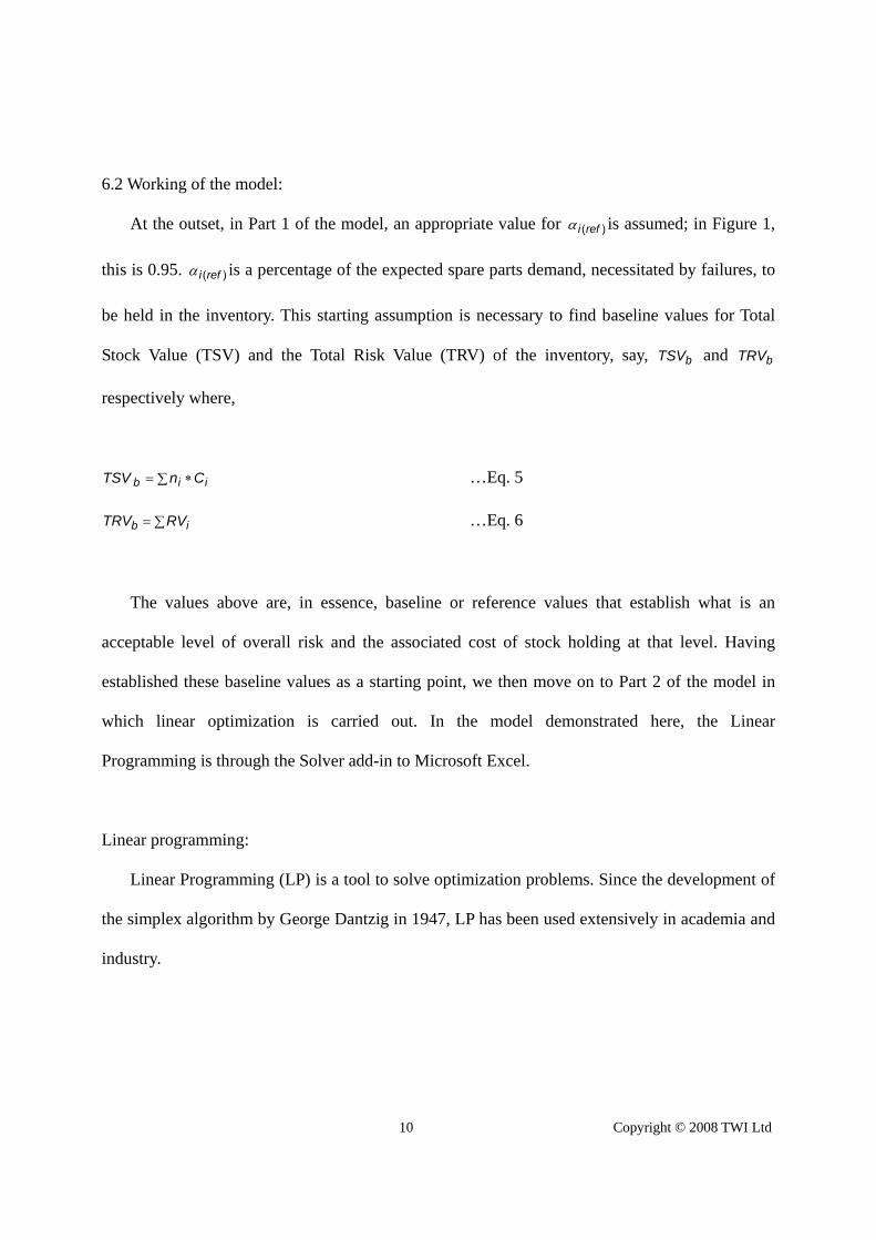
10 Copyright © 2008 TWI Ltd
6.2 Working of the model:
At the outset, in Part 1 of the model, an appropriate value for )(refi is assumed; in Figure 1,
this is 0.95. )(refi is a percentage of the expected spare parts demand, necessitated by failures, to
be held in the inventory. This starting assumption is necessary to find baseline values for Total
Stock Value (TSV) and the Total Risk Value (TRV) of the inventory, say, bTSV and bTRV
respectively where,
bTSV ii Cn …Eq. 5
bTRV iRV …Eq. 6
The values above are, in essence, baseline or reference values that establish what is an
acceptable level of overall risk and the associated cost of stock holding at that level. Having
established these baseline values as a starting point, we then move on to Part 2 of the model in
which linear optimization is carried out. In the model demonstrated here, the Linear
Programming is through the Solver add-in to Microsoft Excel.
Linear programming:
Linear Programming (LP) is a tool to solve optimization problems. Since the development of
the simplex algorithm by George Dantzig in 1947, LP has been used extensively in academia and
industry.

11 Copyright © 2008 TWI Ltd
Formally, a LP problem is an optimization problem for which we do the following:
i) We attempt to maximize (or minimize) a linear function of the decision variables (variables that
describe the decisions to be made). The function that is to be maximized or minimized is called
the objective function.
ii) The values of the decision variables must satisfy a set of constraints. Each constraint must be a
linear equation or a linear inequality.
iii) A sign restriction is associated with each variable. For any variable ix , the sign restriction
specifies either that ix must be nonnegative ( 0ix ) or that ix may be unrestricted in sign. (12)
The optimization here is as follows:
Minimize TSV such that bTRVTRV
All values are integers and greater than zero. The optimized values for TSV and TRV are
oTSV and oTRV respectively.
The Table shows values corresponding to two values of )(refi , 0.95 and 0.90. Consider the first
row in the Table. This scenario is captured by Figures 1 and 2.
Figure 1 shows the risk profile of the various components in the last column. Individual values of
stockout consequence and frequency estimates can also be seen. Figure 2 graphically depicts the
risk profile before and after optimization.
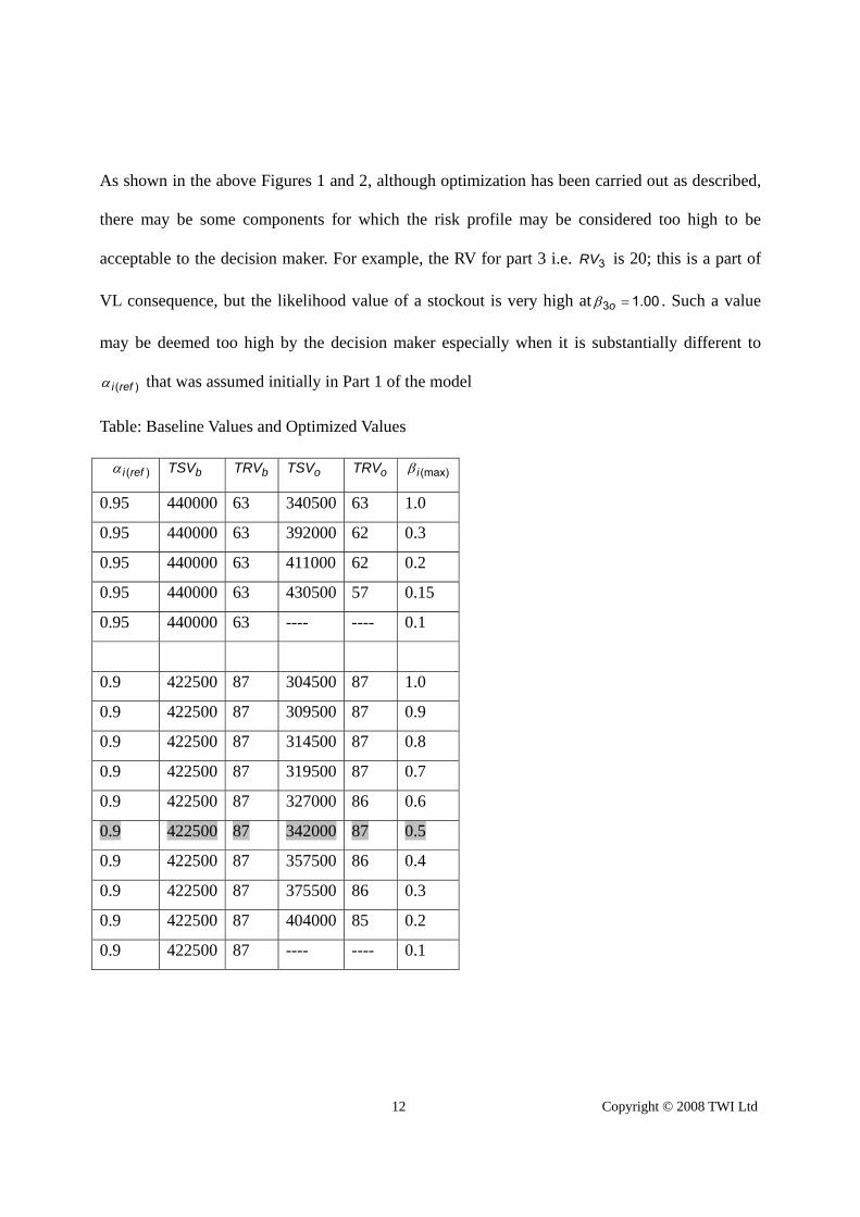
12 Copyright © 2008 TWI Ltd
As shown in the above Figures 1 and 2, although optimization has been carried out as described,
there may be some components for which the risk profile may be considered too high to be
acceptable to the decision maker. For example, the RV for part 3 i.e. 3RV is 20; this is a part of
VL consequence, but the likelihood value of a stockout is very high at 00.13 o . Such a value
may be deemed too high by the decision maker especially when it is substantially different to
)(refi that was assumed initially in Part 1 of the model
Table: Baseline Values and Optimized Values
)(refi bTSV bTRV oTSV oTRV (max)i
0.95 440000 63 340500 63 1.0
0.95 440000 63 392000 62 0.3
0.95 440000 63 411000 62 0.2
0.95 440000 63 430500 57 0.15
0.95 440000 63 ---- ---- 0.1
0.9 422500 87 304500 87 1.0
0.9 422500 87 309500 87 0.9
0.9 422500 87 314500 87 0.8
0.9 422500 87 319500 87 0.7
0.9 422500 87 327000 86 0.6
0.9 422500 87 342000 87 0.5
0.9 422500 87 357500 86 0.4
0.9 422500 87 375500 86 0.3
0.9 422500 87 404000 85 0.2
0.9 422500 87 ---- ---- 0.1

13 Copyright © 2008 TWI Ltd
0
5
10
15
20
25
30
1 2 3 4 5 6 7 8 9 10
Part number
Ris
k va
lue
Original risk value Optimized risk value
Figure 2: Risk Value of parts before and after Optimization
Similarly, the risk level of Part 2 may be deemed unacceptable to the decision maker. To
rectify this, one more constraint is added to the above optimization process by way of adding a
maximum acceptable stockout likelihood value, (max)i .This means that however low impact a
failure to meet a demand for a part is, a minimum stock level will be maintained. (max)i for the
scenario with values as indicated in the first row of the Table is 1.0 i.e. there is no upper limit to
the stockout likelihood. In the subsequent values, (max)i is changed to assess the impact on other
parameters of interest.
As a contrast to the above scenario (indicated in the first row of the Table), Figures 3 and 4
show the results when )(refi =0.95 and (max)i is 0.15 (scenario indicated in the fourth row of the
Table). As shown, with an introduction of a constraint (max)i = 0.15, there is an increase in oTSV
and a decrease in oTRV . The increase in oTSV reflects the extra expense involved in maintaining
a minimum level of inventory and the decrease in oTRV reflects the decreasing risk profile of
spares as stock holding is made to increase consistent with smaller values of (max)i .

14 Copyright © 2008 TWI Ltd
In the Table, for some scenarios there is no optimal solution for the associated baseline TSV
and TRV. This is indicated by ---- in the respective cells of the Table.
Figure 3: Model with maximum acceptable stockout constraint
The Table shows how the optimized values of TSV and TRV change when (max)i values are
changed. To provide a better perspective, two values of )(refi have been used.
(max)i

15 Copyright © 2008 TWI Ltd
0
5
10
15
20
25
1 2 3 4 5 6 7 8 9 10
Part number
Ris
k va
lue
Original risk value Optimized risk value
Figure 4: Risk Value of parts before and after Optimization
It is observed that as (max)i decreases, there is an increase in oTSV and a general decrease in
the oTRV values. oTSV values increase as a minimum level of inventory has been stipulated
regardless of the risk profile of a part. oTRV values tend to decrease as the risk of stockout
decreases. However, in one instance, shown by the highlighted row in the Table, somewhat
counter intuitively and against the trend, the oTRV increases. This is probably due to the constraint
in the linear optimization that the optimum number of parts should be an integer.
Change in Risk Value of parts with change in Beta values
0
5
10
15
20
25
30
1(M) 1000
2(M) 4500
3(VL) 8000
4(VH) 6000
5(VH)10000
6(L) 2000
7(M) 1000
8(H) 3000
9(VL) 3500
10(M) 6000
Part Number (Consequence Value) Cost Price
Op
tim
ized
Ris
k V
alu
e
βi(max)= 0.15 βi(max)= 0.20 βi(max)= 0.30 βi(max)= 1.00
Figure 5: Effect of Beta on optimized individual Risk Values of parts in the Spares Inventory
15.0(max)i

16 Copyright © 2008 TWI Ltd
Figure 5 above shows the impact of change in Beta values on individual optimized Risk
Values of parts. Here, the model described above was run for four values of Beta i.e., 0.15, 0.20,
0.30 and 1.00. (max)i = 0.15 means that an expected stockout likelihood of up to 15% is
acceptable; (max)i = 1.00 means that a total absence of stock of any spare is acceptable. The risk
profiles of the ten parts (depicted by their Risk Values on the vertical axis) are shown. The
horizontal axis depicts Part Number, the Consequence Value in brackets and the Cost Price of that
part. For example, 1 (M) 1000, the first entry on the horizontal axis, stands for Part 1 with M
Consequence Value and a Cost Price of 1000. For Part 1, the Risk Value reduces to zero as Beta
increases. This is because the part is relatively of M consequence and cheap. With increase in
Beta values, money is freed from elsewhere for this part to be stocked more. The same logic
holds true for Part 2. Part 3 is expensive although of VL consequence. Hence an increase in Beta
values raises its optimized Risk Value. Part 4 is accorded top priority as it is of VH consequence
and is somewhat relatively cheaper. Part 5 is of VH consequence but because of its high cost
cannot be stocked at the level of Part 4. Hence it has a Risk Value greater than that of Part 4 for
different values of Beta. If one analyses other parts in Figure 5, the logic behind the methodology
emerges.
This discussion shows how a decision maker can get various perspectives on the risk profile
of the inventory by using this methodology. The model shown here returns a list of optimal
number of units of spares to be held in an inventory such that i) the corresponding expenses are
minimized ii) the overall risk profile of the system (the inventory) is less than the reference one
and iii) the risk associated with individual parts is less than a specified value.

17 Copyright © 2008 TWI Ltd
7.0 SOME LIMITATIONS AND FURTHER RESEARCH
The consequence or impact of a failure to meet a demand for a spare is a qualitative
assessment in the model described above. It is worth noting that the same model will work by
directly putting in the likely impact cost (in monetary terms) of a failure to meet a demand for a
particular spare. However, it is at times difficult to quantify the full implications of such an event.
Therefore, such qualitative assessments, despite the subjectivity involved, are often the best way
to fully estimate the impact of an event. One can make such estimates more precise by fine tuning
the consequences part of the risk estimate. For example, CoF (Consequence of Failure to meet a
demand) can be a weighted sum of various consequences factor values such as: extra cost of
procuring a part on an urgent basis and the lead time under such circumstances, availability of
technical personnel to effect repairs, knock on effect of failure to meet a part on the general
availability of the system and the risk of obsolescence of a part or the machine itself. The
Appendix shows how such an approach can be developed. The approach consists of the following
main steps: (1) Identify factors that impinge on a failure to meet a demand for a spare- impact
factors (IF) - for each spare under consideration. In the table in the Appendix, these are lead time,
availability of technical staff, knock-on failures and associated demands, potential for machine or
spare redundancy and obsolescence (2) Ascribe weights to each of these impact factors to reflect
their relative importance. In the table, these are 10, 10, 60, 15, and 5 for IF1 through to IF5
respectively. (3) Determine relative importance values for VH, H, M, L or VL representing Very
High, High, Medium, Low and Very Low. These are shown to be 100, 80, 60, 40 and 20
respectively. (4) The spare is then assessed qualitatively- VH, H, M, L or VL - under each of the
impact factors identified in step (1). The net result of this exercise is an aggregate Impact Value.
This is ‘84’ in the example shown in the Appendix. This process is repeated for each spare that is
18 Copyright © 2008 TWI Ltd
under consideration in an inventory. The relative weights or values in step (2) and step (3) may or
may not be the same for all parts. Indeed, impact factors also may differ with parts.
This model takes an expected demand for a period as given; the model in its current form is
thus based on periodic reviews. The forecast can be made continuous by using a moving average
method for the demand trend which can make this a continuous review model that may be more
advantageous in some circumstances. The model can also be configured to take in probabilistic
distributions as demand forecast. A more advanced version of this model is being developed
along these lines.
More work needs to be done to show how the approach shown here can be used in
conjunction with more conventional ones such as the Economic Order Quantity (EOR) and the
Materials Requirement planning (MRP) approaches.
Attempts are underway to implement this methodology and present a case study.
8.0 CONCLUSIONS
This paper applies risk based principles to spares inventory management. It extends the risk
based approach that is well established in other areas of industry and used for planning activities
such as maintenance and inspection within process industry. Based on the risk profile of each
part, the model shown here presents the most optimal combination of spares to be held in an
inventory such that the cost of holding such an inventory is minimized subject to a stipulated
maximum individual risk of a stockout of a part and an overall risk of stockout within a system.
The approach outlined here has the potential to increase plant or system availability and manage
business as well as operational risks. It is thus of interest to a number of industry stakeholders
including operators, maintenance personnel, regulators and insurance companies.
19 Copyright © 2008 TWI Ltd
9.0 ACKNOWLEDGEMENTS
This research has been funded by the Centre for Innovative and Collaborative Engineering
(CICE) at Loughborough University, UK in collaboration with TWI Ltd at Cambridge, UK via
the Engineering Doctorate (EngD) scheme. Inspiration for developing this methodology came
from a real life problem in the shipping sector brought to the notice of the lead author, courtesy of
Lloyd’s Register, London, UK.
REFERENCES
(1) ASME: Risk Based Methods for Equipment Life Management: A Step-by-Step Instruction
Manual with Sample Applications (2003)
(2) API: Risk-based Inspection, Recommended Practice 580, 2002, American Petroleum Institute,
USA
(3) API: Risk Based Inspection, Base Resource Document, 2000, 5-1-5-4, American Petroleum
Institute, USA
(4) Risk Based Inspection- A Guide to Effective Use of the RBI Process, The Engineering
Equipment and Materials User’s Association, EEMUA, 2006, No 206:2006
(5) Kennedy,W.J., Wayne Patterson,J., Fredendall,Lawrence D. International Journal of
Production Economics, 2002, 76, 2, 201-215
(6) Zomerdijk, Leonieke G., De Vries, Jan, International Journal of Production Economics, 2003,
81-82, 173-183

20 Copyright © 2008 TWI Ltd
(7) Prasad, Sameer, International Journal of Production Economics, 1993, 34, 209-222
(8) Winston, L. Wayne, Introduction to Operations Research, 1993, 3rd Edition, Duxbury Press,
California, USA
(9) Nahmias, Steven, TIMS Studies in the Management Sciences, 1981, 16, 253-277
(10) Clemen, Robert T., Winkler, Robert L., Risk Analysis, 1999, 19
(11) ASME: Risk Based Methods for Equipment Life Management: A Step-by-Step Instruction
Manual with Sample Applications (2003), Chapter 9: Obtaining and Combining Data
(12) Winston, L. Wayne, Introduction to Operations Research, 1993, 3rd Edition, Duxbury Press,
California, USA, Chapter 3.1: What is a Linear Programming Problem?

21 Copyright © 2008 TWI Ltd
APPENDIX
DERIVING CONSEQUENCE VALUE FOR A PART FROM A NUMBER OF CONSEQUENCE (IMPACT)
FACTORS
Where,
the value ‘8’ in the first column is
(10*80)/100
Weights need to total 100 as this is a relative
assessment
The weighted total ‘84’ is the CoF value for
that part

Appendix C: Paper 3
APPENDIX C : PAPER 3
Bharadwaj, U.R., Wintle, J.B., Silberschmidt, V.V. & Andrews, J.D. 2009, "Optimisation of
resources for managing competing risks", 10th International conference on Engineering
Structural Integrity Assessment, EMAS, 19-20 May, 2009, Manchester, UK.

Risk Based Life Management of Offshore Structures and Equipment

E S I A 1 0
E n g i n e e r i n g S t r u c t u r a l I n t e g r i t y A s s e s s m e n t : p r e s e n t g o a l s – f u t u r e c h a l l e n g e s
1
© EMAS Publishing 2009
* Corresponding Author; Loughborough University/ C/o TWI Ltd, Granta Park, Cambridge CB21 6AL; [email protected] °Loughborough University, UK
OPTIMISATION OF RESOURCES FOR MANAGING COMPETING RISKS
Ujjwal R Bharadwaj*;
John B Wintle; V V Silberschmidt; John D Andrews
The model for managing risk presented in this paper was developed to address the problem of
how many parts of different kinds of a major industrial enterprise should advance in order for
stock to operate at optimum efficiency given that failures may occur in service. The particular
application was a fleet of cargo ships where parts of different kinds are required to keep ships
available for service. For example, spare propellers are expensive items to hold in stock, but
the consequential costs of not having a spare when required can also be expensive. There is an
optimum number of propellers that it is worth holding in order to balance the cost of stocking
too many against the risk of a stock-out. Such risk optimization techniques, in general, find
the optimum trade-off between the cost of a risk mitigating measure and the expected value of
risk without that measure. They have the potential of being applied more widely within
structural integrity and asset management, in any situation where competing risks need to be
managed within finite resources. They may therefore find application in areas such as risk
based inspection and more generally in other areas of risk management.

E S I A 1 0
E n g i n e e r i n g S t r u c t u r a l I n t e g r i t y A s s e s s m e n t : p r e s e n t g o a l s – f u t u r e c h a l l e n g e s
2
© EMAS Publishing 2009
INTRODUCTION
The level of spares in an inventory has a direct bearing on machine availability. The
availability of a machine is a function of the mean time to correct a failure which in turn
depends upon, among other factors, the time to obtain a spare (to conduct repairs) or a
replacement. The level of spares in a spares inventory is constrained by the cost of holding
stock and the penalty of being out of stock. In a competitive climate companies strive to keep
their spares inventory at an optimum level to minimize the costs involved. This paper presents
a new approach - a risk based approach - to spares inventory management aimed at
establishing an optimum level of spares such that financial benefit is maximized within
accepted levels of risk, and the remaining (residual) risks are clearly identified. The paper
presents a framework that enables consistent and auditable decision making in spares
inventory management.
Risk based approaches are used in many sectors of industry and for prioritizing different
types of actions; for example, there are risk based approaches in the process industry to
manage maintenance and inspection and there are standards or guidance documents to
implement these approaches (ASME [1], API [2], API [3] and EEMUA [4]). As opposed to
other approaches, in a risk based approach, actions are based on the risk estimate of various
options. In the current context, this means maintaining an inventory at an optimal level
depending on the risk profile of the spares in which the likelihood of a failure to meet the
demand for a spare is considered in conjunction with the consequences of the failure to meet

E S I A 1 0
E n g i n e e r i n g S t r u c t u r a l I n t e g r i t y A s s e s s m e n t : p r e s e n t g o a l s – f u t u r e c h a l l e n g e s
3
© EMAS Publishing 2009
that demand. The optimal level is such that financial benefits are optimized given risk
associated constraints.
The paper discusses some of the unique features of spares inventories vis-à-vis other types
of inventories. There is also a section on typical costs associated with inventories followed by
a brief note on the main principles underlying various current approaches to spares inventory
management. The main body of the paper then presents the risk based methodology and the
basic model that has been created to implement that methodology. This is followed by
possible areas of further research and conclusions.
SPARE PARTS INVENTORIES
Spare parts inventories are maintenance inventories; they are used by maintenance personnel
to keep machines available and exist to meet an internal demand for spares. They perform a
different function compared to other inventories such as Work-in-progress (WIP) inventories
and Finished Product Inventories. WIP inventories smooth out irregularities in production
flow. These irregularities are caused by factors such as changes in product mix, equipment
breakdowns, differences in production rates, between processes and material handling.
Finished Product Inventories provide a buffer stock to protect against lead time demand,
differences in quality levels, differences in machine production rates, labor troubles,
scheduling problems, gap between capacity and demand and other well established production
problems, Kennedy [5].
Characteristics of spare parts inventories: Spares inventories are hugely influenced by
maintenance policies rather than customer usages that dictate WIP or Finished Product
Inventories. For scheduled maintenance, the demand for spares is relatively more predictable

E S I A 1 0
E n g i n e e r i n g S t r u c t u r a l I n t e g r i t y A s s e s s m e n t : p r e s e n t g o a l s – f u t u r e c h a l l e n g e s
4
© EMAS Publishing 2009
and it may be possible to order parts to arrive just in time for use and indeed not stock such
parts at all. For unplanned maintenance, a lack of some safety stock often means that the
consequences of not keeping some safety stock include production loss. There are other
factors such as the amount of redundancy within a system, availability of reliability
information from condition monitoring equipment, dependency of failure events, possibility
of demands being met by cannibalism and the effect of parts or machine obsolescence on the
level of stock holding. There has also been research illustrating how other factors such as the
organizational context of inventories, especially the responsibilities and authorities of the
persons concerned, have a bearing on inventory management, Zomerdijk and Jan [6].
SOME TYPICAL COSTS ASSOCIATED WITH INVENTORIES
Ordering and setting up costs: These are fixed costs that do not depend on the size of the
order. For example, ordering costs would include paperwork and billing associated with the
order. For parts made in-house, ordering and set up costs would include the cost of labor,
setting up and shutting down the associated machinery.
Unit purchasing cost: This is the variable unit cost of a part or a component. If the part is
manufactured in-house, it includes the variable labor cost, the overhead cost, and the raw
material cost needed to produce a single unit. If this part is ordered from an external source,
then the unit purchase cost must include the shipping cost.
Holding or carrying cost: These are essentially the inventory costs expressed in monetary
value per unit part per year. It includes storage cost, insurance cost, taxes on inventory, and
cost due to the possibility of spoilage, theft, or obsolescence. However, usually the most
significant of the holding cost is the opportunity cost incurred by tying up capital in inventory.

E S I A 1 0
E n g i n e e r i n g S t r u c t u r a l I n t e g r i t y A s s e s s m e n t : p r e s e n t g o a l s – f u t u r e c h a l l e n g e s
5
© EMAS Publishing 2009
The opportunity cost is the return the company would expect on an investment elsewhere
rather than in stock-holding.
Stockout costs: When a demand for a product or a part is not met on time, a stockout is
said to have occurred. If it is acceptable for demands to be met at a later date, no matter how
much later, it is said that demands may be back-ordered. In the current context, risk is the
combination of the probability of a stockout event and its consequence, where a stockout is an
event in which a spare is not available on demand. If it is necessary for demands to be met on
time, and if this is not achieved, then the scenario is a lost case one. In the current context, a
lost case may result in production loss, regulatory penalty and other consequences such as
loss of goodwill. Usually it is more difficult to measure the cost of a stockout rather than
ordering, purchasing or holding costs.
APPROACHES TO INVENTORY MANAGEMENT
There are different approaches to Inventory Management. Prasad [7] categorizes inventory
models into two: Economic Order Quantity (EOQ) and Materials Requirement Planning
(MRP). Under these, he classifies about ninety inventory models. The basic model in an EOR
method determines, subject to a number of assumptions, an ordering policy that minimizes the
yearly sum of ordering cost, purchasing cost, and the holding cost of a part in the inventory.
The basic model in an MRP based method considers the relationship between a component
that is demanded and other associated (sub) components that also need to be available in order
to fulfill that demand.
Winston [8] classifies models as Deterministic EOQ Models, Probabilistic Models and
other recent models such as MRP, Just-in-time (JIT) and Exchange Curves. Nahmias [9]

E S I A 1 0
E n g i n e e r i n g S t r u c t u r a l I n t e g r i t y A s s e s s m e n t : p r e s e n t g o a l s – f u t u r e c h a l l e n g e s
6
© EMAS Publishing 2009
looks specifically at repairable inventory systems and classifies existing models into three
general classes: continuous review, periodic review and models based on cyclic queuing
systems. The Risk Based approach presented here is unique in that it does not completely fall
in any of these categories although it might have some elements of the approaches listed
above.
THE RISK BASED APPROACH TO SPARE PARTS INVENTORY MANAGEMENT
In the current context, the following terms have a special meaning: Risk is the combination of
the probability of a stock out event and its consequence where a stockout is an event when a
spare is not available on demand. Qualitative Risk Analysis broadly covers methods that use
engineering judgment and experience as the bases for the analysis of probabilities and
consequences of failure. Failure Modes, Effects, and Criticality Analysis (FMECA) and
Hazard and Operability Studies (HAZOPs) are examples of qualitative risk analysis that
become quantitative risk analysis when consequences and failure probability values are
estimated. Quantitative Risk Analysis a) identifies and delineates the combinations of events
that, if they occur lead to an undesired event b) estimates the frequency of occurrence for each
combination c) estimates the consequences. The approach shown here is a semi-quantitative
approach that captures best estimates from experts as well as raw historical data. The risk
referred here is relative risk which is a comparative risk of components or equipment in
relation to each other.
In the method described below, a risk profile of the spares is obtained by considering the
likelihood of a failure to meet the demand for a spare in conjunction with the consequences of
the failure to meet that demand. This risk profile is then used to find the optimal level of
inventory such that financial benefit is maximized given an identified acceptable risk level.
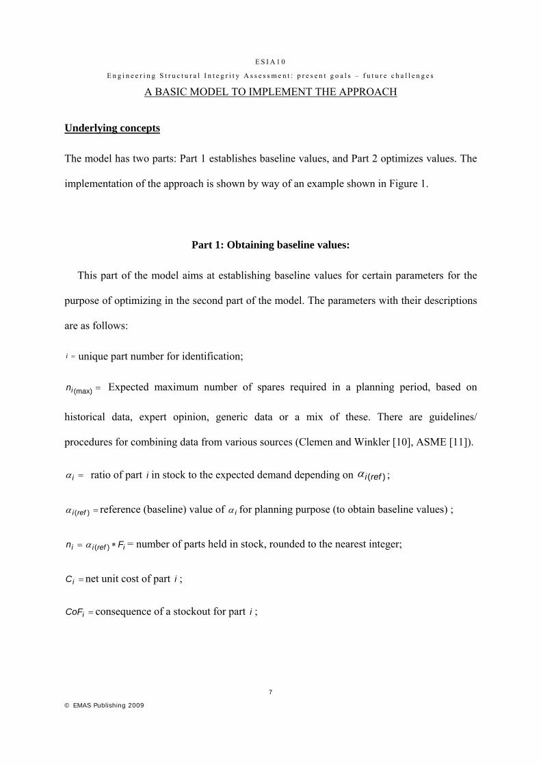
E S I A 1 0
E n g i n e e r i n g S t r u c t u r a l I n t e g r i t y A s s e s s m e n t : p r e s e n t g o a l s – f u t u r e c h a l l e n g e s
7
© EMAS Publishing 2009
A BASIC MODEL TO IMPLEMENT THE APPROACH
Underlying concepts
The model has two parts: Part 1 establishes baseline values, and Part 2 optimizes values. The
implementation of the approach is shown by way of an example shown in Figure 1.
Part 1: Obtaining baseline values:
This part of the model aims at establishing baseline values for certain parameters for the
purpose of optimizing in the second part of the model. The parameters with their descriptions
are as follows:
i unique part number for identification;
(max)in Expected maximum number of spares required in a planning period, based on
historical data, expert opinion, generic data or a mix of these. There are guidelines/
procedures for combining data from various sources (Clemen and Winkler [10], ASME [11]).
i ratio of part i in stock to the expected demand depending on )(refi ;
)(refi reference (baseline) value of i for planning purpose (to obtain baseline values) ;
in irefi F)( = number of parts held in stock, rounded to the nearest integer;
iC net unit cost of part i ;
iCoF consequence of a stockout for part i ;

E S I A 1 0
E n g i n e e r i n g S t r u c t u r a l I n t e g r i t y A s s e s s m e n t : p r e s e n t g o a l s – f u t u r e c h a l l e n g e s
8
© EMAS Publishing 2009
i Stockout frequency estimate for part i , assuming stock outs are proportional to stock
levels
=)
1(maxi
i
n
n = )()( (max)iiii nxnPxP (1)
where )( ixP the probability of a stockout given that a) a quantity ix of that part may be
required during the timeframe i.e. demand for that part b) in is the quantity in stock c)
(max)in being the maximum expected requirement of part i ; this is assuming that the demand
for spares follows a uniform distribution.
iRV Risk value associated with part i
= (Quantified iCoF ) i (2)
TSV ii Cn (3)
TRV iRV (4)
In the model shown above, qualitative estimates of iCoF , VH, H, M, L, VL have been
assigned values 100, 80, 60, 40 and 20 respectively. In a more advanced model, these values
would be a weighted average of values obtained by considering a number of consequence or
impact factors. One such possible scheme is shown in the Figure 5.
Part 2: Obtaining optimized values:
This part of the model contains optimized values obtained after using a linear optimizing
tool using the values in Part 1 of the model, wherever applicable. The optimized values
contain the subscript ‘o’. For example, ion is the optimized value of units of part i to be held
in the inventory.

E S I A 1 0
E n g i n e e r i n g S t r u c t u r a l I n t e g r i t y A s s e s s m e n t : p r e s e n t g o a l s – f u t u r e c h a l l e n g e s
9
© EMAS Publishing 2009
Working of the model:
At the outset, in Part 1 of the model, an appropriate value for )(refi is assumed; in Figure
1, this is 0.90. )(refi (shown in the highlighted box with a small circle towards its top right
corner) is a percentage of the expected spare parts demand, necessitated by failures, to be held
in the inventory. This starting assumption is necessary to find baseline values for Total Stock
Value (TSV) and the Total Risk Value (TRV) of the inventory, say, bTSV and bTRV
respectively where,
bTSV ii Cn (5)
bTRV iRV (6)
The values above are, in essence, baseline or reference values that establish what is an
acceptable level of overall risk and the associated cost of stock holding at that level. Having
established these baseline values as a starting point, we then move on to Part 2 of the model in
which linear optimization is carried out. In the model demonstrated here, the Linear
Programming is through the Solver add-in to Microsoft Excel.
The optimization here is as follows:
Minimize TSV such that bTRVTRV . All values are integers and greater than zero. The
optimized values for TSV and TRV are oTSV and oTRV respectively.
Figure 1 shows the risk profile of various components in the last column. The figure shows
Stockout Risk values associated with )(refi 0.90 both before and after optimization.
Modes of operation:
(A) Minimize Total Risk
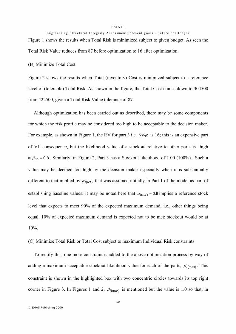
E S I A 1 0
E n g i n e e r i n g S t r u c t u r a l I n t e g r i t y A s s e s s m e n t : p r e s e n t g o a l s – f u t u r e c h a l l e n g e s
10
© EMAS Publishing 2009
Figure 1 shows the results when Total Risk is minimized subject to given budget. As seen the
Total Risk Value reduces from 87 before optimization to 16 after optimization.
(B) Minimize Total Cost
Figure 2 shows the results when Total (inventory) Cost is minimized subject to a reference
level of (tolerable) Total Risk. As shown in the figure, the Total Cost comes down to 304500
from 422500, given a Total Risk Value tolerance of 87.
Although optimization has been carried out as described, there may be some components
for which the risk profile may be considered too high to be acceptable to the decision maker.
For example, as shown in Figure 1, the RV for part 3 i.e. oRV3 is 16; this is an expensive part
of VL consequence, but the likelihood value of a stockout relative to other parts is high
at 8.03 o . Similarly, in Figure 2, Part 3 has a Stockout likelihood of 1.00 (100%). Such a
value may be deemed too high by the decision maker especially when it is substantially
different to that implied by )(refi that was assumed initially in Part 1 of the model as part of
establishing baseline values. It may be noted here that 9.0)( refi implies a reference stock
level that expects to meet 90% of the expected maximum demand, i.e., other things being
equal, 10% of expected maximum demand is expected not to be met: stockout would be at
10%.
(C) Minimize Total Risk or Total Cost subject to maximum Individual Risk constraints
To rectify this, one more constraint is added to the above optimization process by way of
adding a maximum acceptable stockout likelihood value for each of the parts, (max)i . This
constraint is shown in the highlighted box with two concentric circles towards its top right
corner in Figure 3. In Figures 1 and 2, (max)i is mentioned but the value is 1.0 so that, in
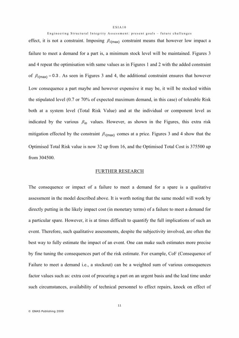
E S I A 1 0
E n g i n e e r i n g S t r u c t u r a l I n t e g r i t y A s s e s s m e n t : p r e s e n t g o a l s – f u t u r e c h a l l e n g e s
11
© EMAS Publishing 2009
effect, it is not a constraint. Imposing (max)i constraint means that however low impact a
failure to meet a demand for a part is, a minimum stock level will be maintained. Figures 3
and 4 repeat the optimisation with same values as in Figures 1 and 2 with the added constraint
of 3.0(max) i . As seen in Figures 3 and 4, the additional constraint ensures that however
Low consequence a part maybe and however expensive it may be, it will be stocked within
the stipulated level (0.7 or 70% of expected maximum demand, in this case) of tolerable Risk
both at a system level (Total Risk Value) and at the individual or component level as
indicated by the various io values. However, as shown in the Figures, this extra risk
mitigation effected by the constraint (max)i comes at a price. Figures 3 and 4 show that the
Optimised Total Risk value is now 32 up from 16, and the Optimised Total Cost is 375500 up
from 304500.
FURTHER RESEARCH
The consequence or impact of a failure to meet a demand for a spare is a qualitative
assessment in the model described above. It is worth noting that the same model will work by
directly putting in the likely impact cost (in monetary terms) of a failure to meet a demand for
a particular spare. However, it is at times difficult to quantify the full implications of such an
event. Therefore, such qualitative assessments, despite the subjectivity involved, are often the
best way to fully estimate the impact of an event. One can make such estimates more precise
by fine tuning the consequences part of the risk estimate. For example, CoF (Consequence of
Failure to meet a demand i.e., a stockout) can be a weighted sum of various consequences
factor values such as: extra cost of procuring a part on an urgent basis and the lead time under
such circumstances, availability of technical personnel to effect repairs, knock on effect of

E S I A 1 0
E n g i n e e r i n g S t r u c t u r a l I n t e g r i t y A s s e s s m e n t : p r e s e n t g o a l s – f u t u r e c h a l l e n g e s
12
© EMAS Publishing 2009
failure to meet a part on the general availability of the system and the risk of obsolescence of
a part or the machine itself. Figure 6 shows how such an approach can be developed. The
approach consists of the following main steps: (1) Identify factors that impinge on a failure to
meet a demand for a spare- impact factors (IF) - for each spare under consideration. In Figure
6, these are lead time, availability of technical staff, knock-on failures and associated
demands, potential for machine or spare redundancy and obsolescence (2) Ascribe weights to
each of these impact factors to reflect their relative importance. In the table, these are 10, 10,
60, 15, and 5 for IF1 through to IF5 respectively. (3) Determine relative importance values for
VH, H, M, L or VL representing Very High, High, Medium, Low and Very Low. These are
shown to be 100, 80, 60, 40 and 20 respectively. (4) The spare is then assessed qualitatively-
VH, H, M, L or VL - under each of the impact factors identified in step (1). The net result of
this exercise is an aggregate Impact Value. This is ‘84’ in the example shown in the Figure 5.
This process is repeated for each spare that is under consideration in an inventory. The
relative weights or values in step (2) and step (3) may or may not be the same for all parts.
Indeed, impact factors also may differ with parts.
This model takes an expected maximum demand for a period as given; the model in its
current form is thus based on periodic reviews. The forecast can be made continuous by using
a moving average method for the demand trend which can make this a continuous review
model that may be more advantageous in some circumstances. The model can also be
configured to take in probabilistic distributions as demand forecast. A more advanced version
of this model is being developed along these lines.

E S I A 1 0
E n g i n e e r i n g S t r u c t u r a l I n t e g r i t y A s s e s s m e n t : p r e s e n t g o a l s – f u t u r e c h a l l e n g e s
13
© EMAS Publishing 2009
CONCLUSIONS
This paper applies risk based principles to spares inventory management. It extends the risk
based approach that is well established in other areas of industry. The example illustrates a
technique of managing risk within user specified constraints as applicable to Spares
Inventory. Risks can be minimized subject to a given Budget (Maximum Total Cost), and
Total Costs can be minimized subject to a specified tolerable level of Risk. The optimisation
can be done at a system level (Total Cost and Total Risk) and it can be done at a component
level too, thus affording the user to manage risks at different levels.
The approach outlined here has the potential to increase plant or system availability and
manage business as well as operational risks. It is thus of interest to a number of industry
stakeholders including operators, maintenance personnel, regulators and insurance companies.
The methodology can be used in other areas that impinge on the structural integrity and asset
management such as Inspection and Maintenance where competing risks (of failure) need to
be managed within finite resources.
ACKNOWLEDGEMENTS
This research has been funded by the Centre for Innovative and Collaborative Engineering
(CICE) at Loughborough University, UK in collaboration with TWI Ltd at Cambridge, UK
via the Engineering Doctorate (EngD) scheme. Inspiration for developing this methodology
came from a real life problem in the shipping sector brought to the notice of the lead author,
courtesy of Lloyd’s Register, London, UK.

E S I A 1 0
E n g i n e e r i n g S t r u c t u r a l I n t e g r i t y A s s e s s m e n t : p r e s e n t g o a l s – f u t u r e c h a l l e n g e s
14
© EMAS Publishing 2009
REFERENCES
(1) ASME: Risk Based Methods for Equipment Life Management: A Step-by-Step
Instruction Manual with Sample Applications (2003)
(2) API: Risk Based Inspection, Base Resource Document, 2000, 5-1-5-4, American
Petroleum Institute, USA
(3) API: Risk-based Inspection, Recommended Practice 580, 2002, American Petroleum
Institute, USA
(4) EEMUA: Risk Based Inspection- A Guide to Effective Use of the RBI Process, The
Engineering Equipment and Materials User’s Association, 2006, No 206:2006
(5) Kennedy,W.J., Wayne Patterson,J., Fredendall, Lawrence D. International Journal of
Production Economics, 2002, 76, 2, 201-215
(6) Zomerdijk, Leonieke G., De Vries, Jan, An organizational perspective on inventory
control: Theory and a case study, International Journal of Production Economics, 2003,
81-82, 173-183
(7) Prasad, Sameer, Classification of Inventory models and systems, International Journal of
Production Economics, 1993, 34, 209-222
(8) Winston, L. Wayne, Introduction to Operations Research, 1993, 3rd Edition, Duxbury
Press, California, USA
(9) Nahmias, Steven, Managing Repairable Item Inventory Systems: A Review, TIMS
Studies in the Management Sciences, 1981, 16, 253-277

E S I A 1 0
E n g i n e e r i n g S t r u c t u r a l I n t e g r i t y A s s e s s m e n t : p r e s e n t g o a l s – f u t u r e c h a l l e n g e s
15
© EMAS Publishing 2009
(10) Clemen, Robert T., Winkler, Robert L., Combining Probability Distributions from
Experts in Risk Analysis, Risk Analysis, 1999, Vol. 19, No. 2
(11) ASME: Risk Based Methods for Equipment Life Management: A Step-by-Step
Instruction Manual with Sample Applications (2003), Chapter 9: Obtaining and
Combining Data
(12) Winston, L. Wayne, Introduction to Operations Research, 1993, 3rd Edition, Duxbury
Press, California, USA, Chapter 3.1: What is a Linear Programming Problem?

E S I A 1 0
E n g i n e e r i n g S t r u c t u r a l I n t e g r i t y A s s e s s m e n t : p r e s e n t g o a l s – f u t u r e c h a l l e n g e s
16
© EMAS Publishing 2009
FIGURES
Minimize Total Risk Value or Total CostIndividual Risk Profiles before and after Optimization
0
5
10
15
20
25
1 2 3 4 5 6 7 8 9 10Part No
Ris
k V
alu
e
Original Risk Value Optimized Risk Value
Figure 1: Minimize Total Risk subject to given Budget

E S I A 1 0
E n g i n e e r i n g S t r u c t u r a l I n t e g r i t y A s s e s s m e n t : p r e s e n t g o a l s – f u t u r e c h a l l e n g e s
17
© EMAS Publishing 2009
Minimize Total Risk Value or Total CostIndividual Risk Profiles before and after Optimization
05
1015202530354045
1 2 3 4 5 6 7 8 9 10Part No
Ris
k V
alu
e
Original Risk Value Optimized Risk Value
Figure 2: Minimise Total Cost subject to a tolerable level of Total Risk
Figure 3: Minimize Total Risk subject to given Budget and individual Risk constraints (βi(max))
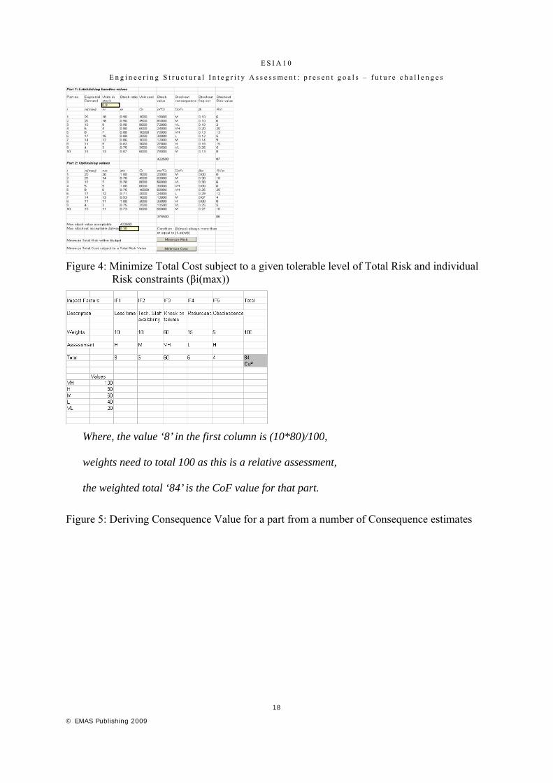
E S I A 1 0
E n g i n e e r i n g S t r u c t u r a l I n t e g r i t y A s s e s s m e n t : p r e s e n t g o a l s – f u t u r e c h a l l e n g e s
18
© EMAS Publishing 2009
Figure 4: Minimize Total Cost subject to a given tolerable level of Total Risk and individual Risk constraints (βi(max))
Where, the value ‘8’ in the first column is (10*80)/100,
weights need to total 100 as this is a relative assessment,
the weighted total ‘84’ is the CoF value for that part.
Figure 5: Deriving Consequence Value for a part from a number of Consequence estimates

Appendix D: Paper 4
APPENDIX D : PAPER 4
Bharadwaj, U.R., Silberschmidt, V.V, Wintle, J.B., "A Risk-based Approach to Asset
Integrity Management”, accepted for publication in the Journal of Quality in Maintenance
Engineering.

Risk Based Life Management of Offshore Structures and Equipment
2
A RISK- BASED APPROACH TO ASSET INTEGRITY MANAGEMENT OF
STRUCTURES AND EQUIPMENT
Bharadwaj, U.R., Silberschmidt, V.V., Wintle, J.B.
Abstract
Purpose
Inspection and maintenance of plant and machinery has traditionally been based on prescriptive
industry practices. However, increased experience and a greater understanding of operational
hazards is leading sections of industry to take a more informed approach to planning inspection
and maintenance, targeting resources to reduce the risk to as low as reasonably practicable. The
purpose of this paper is to present an approach to asset management to minimize risks in the most
cost effective way.
Methodology
The methodology to implement the approach optimizes the decision-making for undertaking run-
repair-replace decisions with the ultimate aim of maximising the Net Present Value (NPV) of the
investment on such actions. The risk-based approach to asset integrity management, as opposed
to the more conventional approaches, assesses failure in its wider context by considering not just
the likelihood of failure, but also the consequences should the failure event occur.
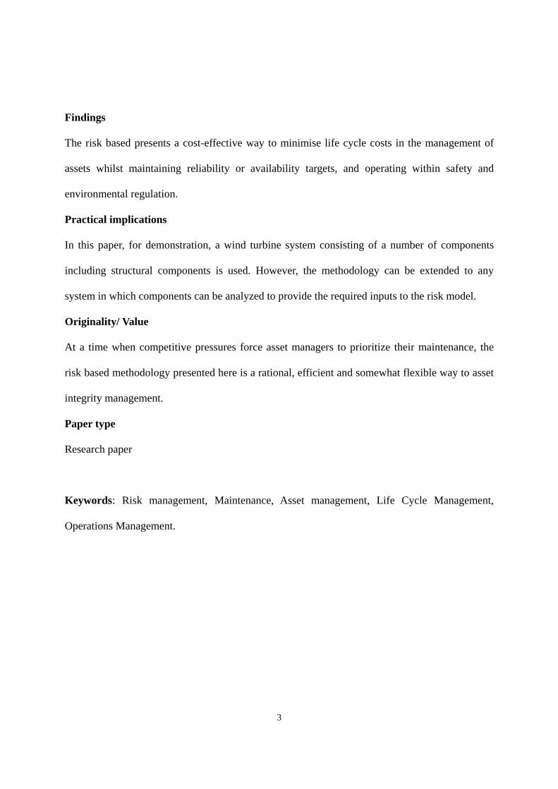
3
Findings
The risk based presents a cost-effective way to minimise life cycle costs in the management of
assets whilst maintaining reliability or availability targets, and operating within safety and
environmental regulation.
Practical implications
In this paper, for demonstration, a wind turbine system consisting of a number of components
including structural components is used. However, the methodology can be extended to any
system in which components can be analyzed to provide the required inputs to the risk model.
Originality/ Value
At a time when competitive pressures force asset managers to prioritize their maintenance, the
risk based methodology presented here is a rational, efficient and somewhat flexible way to asset
integrity management.
Paper type
Research paper
Keywords: Risk management, Maintenance, Asset management, Life Cycle Management,
Operations Management.
4
1. Introduction
Decisions within asset integrity management that include decisions regarding inspection, repair,
maintenance and replacement have traditionally been based on a range of practices including the
prescriptive time-based (rule-based) approach, the condition-based approach, Reliability Centred
Maintenance (RCM) and Reactive Maintenance (RM).
Whilst there will remain the need for traditional approaches to asset integrity management, it is
increasingly felt that more advanced approaches are required to reflect the complexity and
innovation involved in the assets, and to operate at an optimal level within the competitive
pressures faced by asset managers. Risk based approaches, as opposed to many other approaches,
give operators some flexibility in the management of their assets whilst meeting the same
objectives. The flexibility is as a result of undertaking actions not on a fixed schedule or rule, but
on some identified measures of risk. The risk based approach uses risk based criteria to prioritize
efforts and make the optimum use of this flexibility.
The uptake of risk based practices is growing as increased operational experience and a greater
understanding of failures (and its consequences) lead some parts of industry to adopt a more
informed approach to planning, targeting resources to reduce risk to as low as reasonably
practicable. Risk based approaches are used in many sectors of industry and for prioritizing
different types of actions; for example, there are risk based approaches in the process industry to
manage maintenance and inspection and there are standards or guidance documents to implement
these approaches (ASME, 2003; API, 2000; API, 2002; EEMUA, 2006).

5
This paper develops and demonstrates a risk-based methodology to estimate the optimum time of
replacement or repair of a structure, in a system comprising a number of components, within
constraints of the budget available, such that financial benefit of the action taken is maximised.
The paper starts with a discussion on risk and its analysis as applied to asset integrity
management in general, and moves on to the concept of risk measured in terms of expected
values, the concept of NPV, and the trade- off involved in risk-based decision-making within the
constraints that apply.
2. The Risk Based Approach to asset integrity management
Risk
Risk has numerous definitions. Risk is a combination of the probability of an event and its
consequence (API, 2002). It is a deviation from the normal or expected. Numerically, it is a
product of probability of an event occurring and the consequence of the event.
A risk-based approach considers failure taking cognizance of the two elements that constitute risk
- the probability (or likelihood) of failure and the consequence of that failure.
In the context of this paper, risk will involve the probability or the likelihood of failure of a
component or a system of components to fulfil its design purpose in a given time frame and
under given operating conditions. Where the two components of risk i.e. the likelihood and the
consequence of a failure event are quantitatively expressed, risk will be expressed in terms of
‘expected loss’. Expected loss can be defined quantitatively as the product of the consequences
(C) of a specific incident and the probability (P) over a time period or frequency of its occurrence
(Andrews and Moss, 2002):

6
(1)
Risk Analysis methods
Risk analysis methods are generally categorised as qualitative or quantitative. There may be an
intermediate category (semi-quantitative) depending upon how quantitative the risk analysis is.
The API’s Recommended Practice 580 (API, 2002) on risk-based inspection describes a
‘continuum of approaches’ ranging from the qualitative to quantitative. The level of detail in risk
analysis corresponding to a purely qualitative approach, on one end of the spectrum, is low
compared to the purely quantitative one on the other. There are intermediate approaches that may
have both qualitative and quantitative attributes.
Qualitative Analysis
Engineering judgment and experience are the basis for risk assessment in a qualitative analysis.
The results of the analysis largely depend on the expertise of the user. The primary advantage of
qualitative risk analysis is that it enables assessment in the absence of detailed (and entailing the
use of substantial resources) numerical data. It is also the first pragmatic step to conduct a
quantitative risk analysis by screening out components of less concern, and is often the best way
to take a system-wide view. However, it is not a very detailed method and provides only a broad
categorization of risk. Failure Modes, Effects and Criticality Analysis (FMECA) (MIL-STD-
1629, 1980), Hazard and Operability Studies (HAZOPS), and the Risk Matrix approach are
.PCR
7
examples of qualitative methods. In the Risk Matrix, approach, the likelihoods and consequences
of failure are qualitatively described in broad ranges (e.g. high, medium or low).
Quantitative Analysis
Qualitative risk assessments become less discerning when the system complexity increases. So a
quantitative method is often required to achieve risk discrimination of a system of components.
Quantitative Analysis assigns numerical values to the probability (e.g. 10-5 failure events per
year) and the consequences of failure (e.g. revenue loss or inventory released over 1,000 m2).
Qualitative Analysis techniques such as FMECA and HAZOPS can become quantitative when
the values of failure consequence and failure probability are numerically estimated. This can be
performed using a variety of references such as generic failure databases, elicited expert
opinions, or calculated by means of specific engineering and statistical analysis (ASME, 2003).
There are statistical methods for combining data from various sources or updating data with
additional information, (Jordan, 2005), (Kallen and Noortwijk, 2005), (Thodi et. Al., 2009).
In the current discussion, it is assumed that there is a system comprising a number of structures
and a qualitative analysis has identified high-risk components. For the sake of demonstration,
consider the system as a wind turbine (comprising of electrical and structural components).
Among high-risk components- the wind turbine tower structure- has been identified. For
simplicity, wind turbine tower structure will be referred to as ‘structure’ in the discussion below.
The paper now describes a methodology for performing quantitative analysis on the structure that
has been identified as high risk and how the results of this analysis feeds into the planning/

8
decision-making in integrity management of the system. Again, for the sake of simplicity, the
decisions involved are run or replace. However, the same method can be extended to other plan
other actions in asset integrity management such as repair and inspection.
For the quantitative risk analysis method described in this paper, a failure frequency-time curve is
developed by engineering analysis of the structure for the active or potentially active in-service
damage mechanisms. Among the expected damage mechanisms, corrosion is chosen to
demonstrate the methodology. The consequence of failure is in financial terms as it is assumed
that the functioning of the structure is business-critical.
Quantitative consequence analysis
A possible scheme for quantitative assessment of consequences using FMEA is shown in Table 1.
The table is for illustration only. There may be some intangibles remaining or if quantified, may
be approximate assessments; for example, ‘technology confidence loss’ may be quantified in
some way- losing similar projects or a drop in the share value of the company.
In the analysis that follows, for simplicity, the consequence considered and quantified is just the
production loss.
3. Quantitative probabilistic damage mechanism model for failure due to corrosion
This paper does not discuss the details of damage models for use in probabilistic analysis. Instead
it illustrates a simple probabilistic damage mechanism model for general corrosion of the tower
structure. Consider a structure subject to corrosion. For the sake of simplicity, assume that this is

9
the only damage mechanism causing failure of the structure and that there is a breakdown of
coating. The remaining life (RL) of the structure can be calculated as:
CR
MATTcRL
)( (2)
Table 1: Identified consequences and associated costs of damage to a wind turbine tower
where, RL = remaining life (years); Tc = current thickness of the structure (mm);
MAT = minimum allowable thickness to maintain integrity of the structure (mm); and
CR = corrosion rate (mm/year). These terms are explained in more detail later in this section.
If To is the original nominal thickness of the structure, then at the end of t years,
tCRToTc * . (3)
Failure Mode Effect Consequence category Consequence Cost (£k) Source/commentMaintenance durationRegulator penaltiesOther turbinesSea vehicleslocal structuresInjuryDeathInstallation of new structureRepair and recommissionInsurance premiumTechnology confidence lossLost productionMaintenance cost
Keep in serviceMaintenance durationRegulator penaltiesOther turbinesSea vehicleslocal structuresInjuryDeathInstallation of new structureRepair and recommissionInsurance premiumTechnology confidence lossLost productionMaintenance cost
Keep in serviceMaintenance durationRegulator penaltiesOther turbinesSea vehicleslocal structuresInjuryDeathInstallation of new structureRepair and recommissionInsurance premiumTechnology confidence lossLost productionMaintenance cost
Keep in service
Personnel
Maintenance costs
Reputation
Repair
Corrosion - Uniform Band in
Splash Zone
Collapse
Find and Assess
Collapse
Scouring
Fatigue - Circumferential
cracking
Collapse
Find and Assess
Find and Assess
Reputation
Repair
Production loss
Secondary Damage
Personnel
Maintenance costs
Reputation
Repair
Production loss
Secondary Damage
Production loss
Secondary Damage
Personnel
Maintenance costs

10
The reliability of an element of a system can be determined based on a performance function that
can be expressed in terms of basic random variables )( iX for relevant random loads and
structural strength (Ayyub, 2003).
Mathematically, the performance function Z can be described as
LRXXXZ n ),...,( 21 (4)
where, R is the resistance or strength and L is the load.
The limit state can be defined as
(5)
Accordingly, when 0Z , the element is in the failure state, and, when 0Z , it is in the survival
state.
The limit state equation implied in equation (3.2), when remaining life is zero, can be expressed
as
0)*()(
CR
MATtCRT
CR
MATTRL oc
,
0* MATtCRTo , which can be re-arranged to
0]*[][ tCRMATTo . (6)

11
where, the first term represents structural strength (R) , and the second, load effect (L).
A purely deterministic RL model would have each independent variable in equation (2) as a
specific value. This assumes that these variables have no random or probabilistic aspects but can
be defined in a fixed predictable fashion. In reality, there is considerable uncertainty associated
with these variables and each can be defined by a statistical distribution of values.
The corrosion rate (CR) maybe derived from periodic in-service measurements of metal loss
resulting from corrosion or from laboratory tests. In the calculations that follow, CR is assumed
to be a normal distribution with a mean of 0.4mm/year and a standard deviation of 0.1mm/year,
N (0.4, 0.1). These values are for demonstration only. As CR cannot be negative, the distribution
is truncated to so that the lower boundary is greater than or equal to zero.
The RL model has been created using the ‘@Risk’ software from Palisade Corporation. Figure 1
depicts the distribution for CR using the @Risk software. Numbers on the horizontal axis
represent the corrosion rate in mm/year. (The percentage values on the horizontal axis show what
percentage lie in a given range of values- this is not used in the below. The values on the vertical
axis in figure 1 are also not used in the calculation below.) The distribution can also be obtained
from fitting a curve to real values of CR as measured over a period of time and could well be a
different kind of distribution.

12
Normal(0.4, 0.1) Trunc(0,+inf)
0.0
0.5
1.0
1.5
2.0
2.5
3.0
3.5
4.0
-0.1 0.0
0.1
0.2
0.3
0.4
0.5
0.6
0.7
>5.0% 90.0%
0.2355 0.5645
Figure1: Corrosion rate (mm/year) distribution
Current thickness (Tc) is known from the most recent thickness measurements on the structure,
say during the year of assessment. If recent thickness measurements are not available, Tc can be
assumed to be equal to the original nominal thickness of the structure (To) as specified by the
designer including tolerances, corrosion allowance, etc, and the RL calculated from the year of
installation. For the purpose of demonstration, in the model, To is also a normal distribution, N
(100, 1) i.e. with mean=100mm and standard deviation=1mm.
MAT is the absolute minimum allowable thickness calculated by the designer to prevent failure
by overload, collapse, etc as appropriate. In the illustration this value is 90 mm. ‘Failure’ in this
context is not having the minimum allowable design thickness (MAT) rather than actual physical
collapse of the structure. The probability of not meeting MAT is greater than that of structural
13
collapse as there is a factor of safety within the minimum design thickness, making the analysis
conservative.
In the method here, the statistical analysis tool - Palisade’s @RISK for Microsoft Excel is used to
describe all the independent variables probabilistically, and RL is then calculated using Monte
Carlo Simulation (MCS) technique. In this way, the calculated RL by MCS is actually a
distribution of values, so that the annual probability of failure (the failure rate per year) over time
can be obtained. This annual probability of failure, in the current context, is effectively the
proportion of surviving population of structures from the previous year that is expected to fail
within the year under consideration.
Annual probability of failure )0( RLP (7)
For example, see figure 2 that shows an assessment of the annual probability of failure of a tower
structure with (1) an initial (in the year of installation i.e. 2000) thickness of 100 mm with some
deviation described by N(100,1); (2) Expected CR as N(0.4, 0.1) with negative values truncated;
(3) MAT as 90 mm. The number of iterations is set to 1000. This means that for year 2000, 1000
values for CR and Tstart are selected from the respective stipulated distributions. These initial
values are used in calculations for the year 2000 and all the subsequent years.
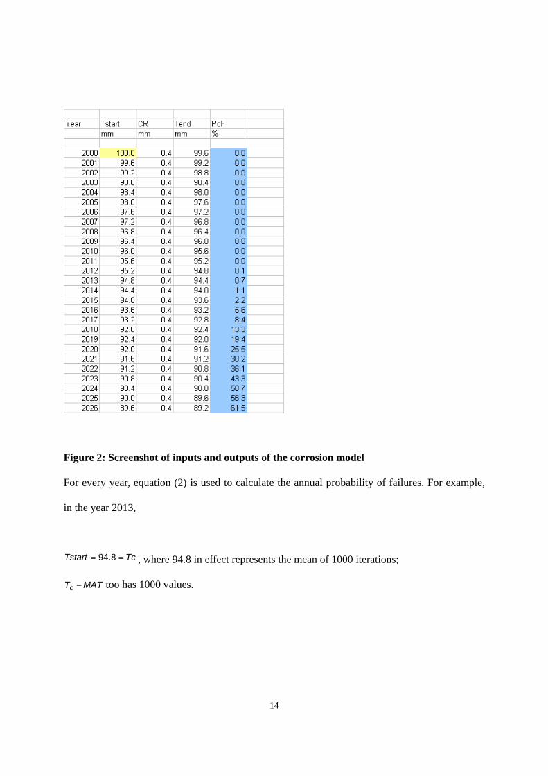
14
Figure 2: Screenshot of inputs and outputs of the corrosion model
For every year, equation (2) is used to calculate the annual probability of failures. For example,
in the year 2013,
TcTstart 8.94 , where 94.8 in effect represents the mean of 1000 iterations;
MATTc too has 1000 values.

15
The algorithm counts the number of times MATTc is negative or zero; in this case 7 times out of
a total of 1000 iterations. These are the times when, as per equation (2), .0RL Percentage
values give )0( RLP as shown in column 5 in figure 2.
This annual probability of failure (failure rate) versus time curve is used in the next stage in
which the timing of an action (repair/ replacement) can be optimised such that financial benefit is
optimised.
Annual probability of failure (PoF) Vs time
0102030405060708090
100
2000 2010 2020 2030 2040 2050
Years
An
nu
al P
oF
(%
)
Figure 3: The annual probability of failure versus time curve

16
4. Risk based financial optimisation of maintenance action given a failure trend
The need for financial criterion in maintenance decision making
Maintenance projects are increasingly being evaluated by decision makers who need to
understand the implications of various options in financial terms. Although predictive
maintenance techniques have matured, the predictions are in engineering terms. Thus, there is a
need to express the effects of engineering wear and tear in financial terms. In the current context,
this is done by evaluating the cost of the consequences of failure owing to wear and tear of plant
and machinery.
The drivers for a consistent decision making methodology in maintenance
Many old plants, structures, capital equipment or components are in their Ageing period of life.
However, increasing competition means many of them cannot be replaced and need to have their
useful life extended. In addition, new components are often designed to operate with maximum
efficiency, and are designed with lower “margins of error” against assumed operating conditions.
Each action (or project) has costs associated with it. These costs are, in essence, investments
made by the concerned asset owner with the expectation of certain return on the investment(s).
The decision maker will normally be faced with a number of projects competing for such
investments, and therefore needs to take decisions that maximise the returns on these investments
within the constraints that apply (Tam and Price, 2008).The most widely understood financial
techniques to evaluate projects include ‘return on investment’, ‘pay-back period’ and ‘discounted
cash flow (DCC)’ methods (Brealey, Myers 1991). These techniques have various strengths and
17
weaknesses. The methodology here employs the net present value (NPV) technique that is a form
of DCC analysis
NPV in financial analysis
In the current discussion, it is assumed that a project with a higher NPV is a better investment
than a project with a lower NPV. The NPV of a project is the present (current) value of the total
future cash flows, i.e. the net of both positive (income) and negative (cost) cash flows. NPV
considers the time value of money by discounting all the cash flows, and it is calculated as
follows:
NPV = tN
tt rC )1()(
0
(8)
N = project life (years); t = timing of cash flow (year); r = interest rate, or discount rate; and Ct =
cash flow in year t.
The future cash flows are ‘expected’ cash flows, as they do not occur with certainty. The
uncertainty arises in the engineering analysis to calculate the probability of failure over time for
the damage mechanism(s) of interest.
The risk associated with any project is expressed in terms of its NPV by using expected values
(EV). The EV of a failure event is the product of the probability of an event occurring and the
cost of consequence of that event. The probability of an event and the cost of the consequence(s)
of that event is directly assessed from prior quantitative analyses; the consequence cost is
expressed in financial terms.

18
Thus, the NPV of a project with uncertain outcomes is the sum of the expected values of all
future discounted cash flows, as follows:
N
t
ttt rCp
0
)1()( (9)
where, pt = the probability of the event occurring at time t.
The risk-based optimisation model
The optimisation maximises the NPV of the action (repair/replacement) under consideration. In
this case, the optimisation finds the least negative value of NPV. Cash inflows are treated as
positive and cash outflows as negative: 1) money spent on an action is negative, 2) failure
consequence costs ((unplanned) outages due to failure mainly production loss considered here,
for simplicity) is also negative, but 3) failure costs avoided by undertaking the action under
consideration are considered positive.
Consider that our planning period is from t=0 to t=N and the year of assessment is t=0. Let us
consider the NPV of an action undertaken in any year t=n. It is given by:
NPV= (Expected present value of action undertaken in year t=n) + (Expected present value of
costs due to outages prior to the action) + (Expected present value of costs due to outages
avoided due the action) (10)
NPV=

19
The first two terms in equation (10) are negative, the third is positive.
Hence,
NPV = { ])1()([ tNt
ntPt rC
+ [- tnt
tBtt rCp )1()(
0
]} + { tNt
ntBtt rCp )1()(
1
] } (11)
In equation (11), for the NPV of an action taken at time t=n, the following can be defined:
CBt = Cash flows associated with production in year t;
CPt = Cash flows associated with implementing the project in year t, including any tax credits
(positive cash flow) on depreciation costs (Collier & Glagola, 1998);
N = the maintenance planner’s strategic planning period, i.e. from t=0 to t=N;
n = year in which the action is proposed to be undertaken;
pt = probability of the event (failure leading to the particular consequence) occurring in year ‘t’;
and
r = interest rate, i.e. the cost of money (finance).
The optimisation algorithm calculates the year of maintenance action for which the NPV is
maximum (least negative, in this case), subject to stipulated constraints.
20
The maintenance action may be replacement or repair. In both cases, it is assumed that the cost of
action includes the cost of initial problems (teething problems) and that once the equipment or
structure is in place and functional, it begins its life cycle at a relatively very low failure rate.
The key inputs to the optimisation model are as follows:
(a) The annual probability of failure versus time values using which expected values are derived
as per the formula discussed above; the failure trend is obtained from quantitative
assessments.
(b) The consequence cost of failure (unplanned outage).
(c) Interest rates and depreciation as applicable.
(d) Any financial constraints, such as the annual maintenance budget limit.
(e) Although not shown in the calculations here, any non-financial constraints, e.g. those on
failure rates due to safety regulations.
5. Demonstration of the model
The approach described above is demonstrated by evaluating three offshore wind turbine tower
structures - structure 1, structure 2 and structure 3. The failure trend from a probabilistic
corrosion model is presented in figures 2 (spreadsheet calculations) and 3 (graphical
presentation). How the Action NPV (depicted by the curve with triangles) changes with the
failure trend (curve with square boxes; the same curve as shown in figure 3) is shown figure 4.
The values are obtained by using equations 10 and 11 for each year in the planning period.
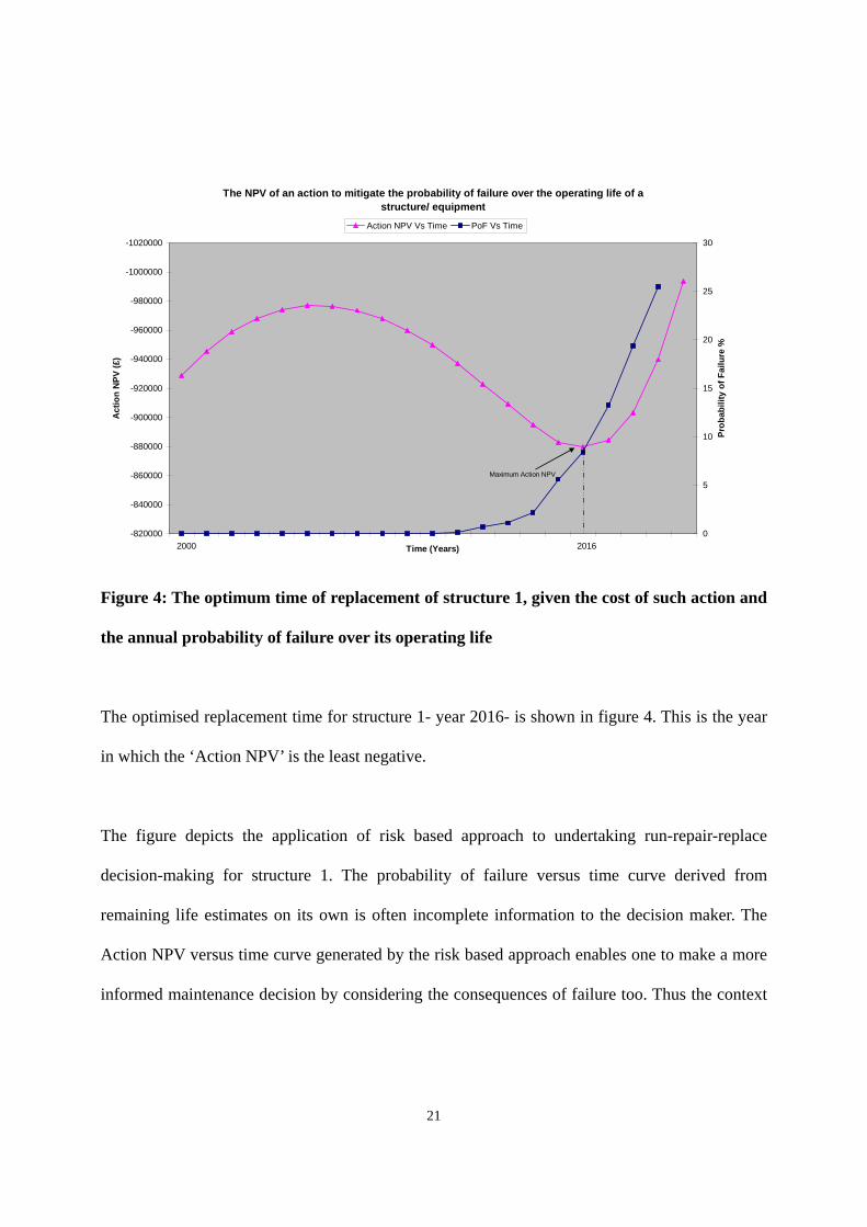
21
The NPV of an action to mitigate the probability of failure over the operating life of a structure/ equipment
-1020000
-1000000
-980000
-960000
-940000
-920000
-900000
-880000
-860000
-840000
-820000
Act
ion
NP
V (
£)
0
5
10
15
20
25
30
Time (Years)
Pro
bab
ilit
y o
f F
ailu
re %
Action NPV Vs Time PoF Vs Time
Maximum Action NPV
20162000
Figure 4: The optimum time of replacement of structure 1, given the cost of such action and
the annual probability of failure over its operating life
The optimised replacement time for structure 1- year 2016- is shown in figure 4. This is the year
in which the ‘Action NPV’ is the least negative.
The figure depicts the application of risk based approach to undertaking run-repair-replace
decision-making for structure 1. The probability of failure versus time curve derived from
remaining life estimates on its own is often incomplete information to the decision maker. The
Action NPV versus time curve generated by the risk based approach enables one to make a more
informed maintenance decision by considering the consequences of failure too. Thus the context

22
in which the structure is operating and the implications of it failing feed into the process of run-
repair-replace decision-making.
The optimised action years for the other two structures are derived in the same way. This is
shown in figure 5. It is seen that both structure 1 and structure 2 have the same year of
replacement- 2016, and structure 3 has 2012 as the year of replacement. The figure shows a
scenario in which the budget for repair/ replacement of structures in a wind farm is set to
maximum of £ 6400,000 in any given year with an increase of 0.05 % every year. It is assumed
that if this budget is not used in a given year on asset management actions within this wind farm,
it is used elsewhere- there is no facility for a rollover. Due to this limit on expenses, if actions are
taken as calculated, there would be deficits in the years in which the actions are taken.
To address this, optimisation is carried out again (using Solver in Microsoft Excel). The re-
scheduled time of action is shown in figure 6. All actions are now within the allocated budget.
However, the change in schedule comes at a price: the NPV decreases from the previously
optimised value of - £ 7118677 to -£ 7148132. To take the analyses one step further this loss in
NPV could be compared to the expected cost of borrowing to see if actions can be taken in the
years as originally identified as the most optimum time.
In-service inspection optimisation
The model could be extended to inspection actions. Instead of the replacement cost of the
component, the cost of in-service inspection would be considered. Since such actions (projects)
are usually accounted for as ‘expenses’ in the year in which they occur, rather than as

23
‘investments’ (which would then be written-off over several years), tax credits from depreciated
costs do not arise. Since inspection costs are relatively low compared to production loss it is
expected that the model would suggest the optimum year of inspection to be the first year of the
planning period. To address this, to optimise in-service inspection dates:
1. Optimise the action date as if the action was replacement,
2. Inspect the equipment before this calculated replacement date,
3. Compare the actual component damage found during inspection, to the projected conditions,
and then
4. Replace the component if necessary, or re-calculate a new optimised replacement date.
6. Discussion
In the RBLM optimisation model presented above, the following points warrant further
discussion:
(1) Multi-component optimisation
It has been shown that the optimum year of replacement can be calculated when the net present
value (NPV) of the maintenance action is maximised. If in a system of structures there is a
budgetary constraint that does not allow for a series of actions to be undertaken in a given
strategic planning period, further optimisation can be undertaken using the approach.

24
(2) Quantitative inputs
The technique requires a quantitative assessment of degradation/ damage. This is at times
expensive, time consuming and requiring simplifying assumptions to be made.
Figure 5: Optimised action schedule leading to budget deficit arising due to two structures
being replaced in the same year (2016)

25
Figure 6: Re-scheduling the year of action such that the costs lie within allocated budget
26
(3) RBLM models in complex systems
For more complex systems with increasing number of components and constraints, non-linear
optimisation tools (e.g. those based on genetic algorithms) that are more powerful than the linear
Solver in Microsoft Excel may be required;
(4) Direction of future relevant work
There is scope for further work on deriving failure estimates using expert elicitation and
combining failure probabilities using Bayesian methods to update prior probability distributions
with other data sources, e.g. combining specific failure databases with expert knowledge. More
research is needed in assessing the use of genetic algorithms for optimisation in complex
systems. Finally, further work is needed to incorporate a wider range of in-service equipment
damage mechanisms to optimise RBLM actions.
7. Conclusions
The paper presents a quantitative risk analysis model to undertake run-repair-replace decisions in
asset integrity management. The model implements an approach that ultimately minimises the
risks associated with failures by optimally targeting resources at those components (within the
asset system) identified as high risk.
8. Acknowledgements
The author wishes to acknowledge the financial support of TWI Ltd and the CICE (Centre of
Innovative and Collaborative Engineering) at Loughborough University for this research.

27
This paper builds on a conference paper presentation by the lead author (Bharadwaj et al, 2007)
and has gained from feedback received. The author is grateful to Chris Ablitt (TWI Ltd) and
Julian B Speck (previously with TWI Ltd) for their perspectives on risk based practices in
industry.
References
Andrews, J.D. & Moss, T.R. 2002, "An Introduction to Reliability and Risk Assessment" in
Reliability and Risk Assessment, Second edn, Professional Engineering Publishing, UK, pp. 9.
API Publication 2002, Risk-based Inspection, API Recommended Practice 580, American
Petroleum Institute, USA.
API Publication, 2000, Risk-Based Inspection, Base Resource Document.
ASME International 2003, Risk Based Methods for Equipment Life Management, CRTD Vol. 41,
ASMW, New York.
Ayyub, Bilal M. (2003) Risk Analysis in Engineering and Economics, Chapter 4: Reliability
Assessment, pp.179-192, Washington: CRC Press.

28
Bharadwaj, U.R., Speck, J.B. & Ablitt, C.J. 2007, "A practical approach to risk based assessment
and maintenance optimisation of offshore wind farms", Offshore Mechanics and Arctic
Engineering (OMAE), ASME, June 10-15, 2007, San Diego, California, USA.
Brealey, R.A. & Myers, S.C.1991, Principles of Corporate Finance, 4th Edition, McGraw-Hill,
New York.7.
Collier, A.C. & Glagola, R.C.1998, “Engineering Economics and Cost Analysis”, 3rd Edition,
Addision-Wesley, California, pp. 438-464.
EEMUA 2006, Risk Based Inspection- A guide to effective use of the RBI process, EEMUA, UK.
Jordon, I., 2005, “Decisions Under Uncertainty: Probabilistic Analysis for Engineering
Decisions”, Cambridge University Press, Cambridge, UK.
Kallen, M.J. & Noortwijk, J.M.V. (2005), “Optimal Maintenance decisions under imperfect
inspection”, Reliability Engineering & System Safety, Volume 90, Issues 2-3, November-
December 2005, Pages 177-185.
MIL-STD-1629A (1980), Military Standard 1629A, Procedures for performing a Failure Mode,
Effects and Criticality Analysis, Department of Defense, Washington DC.

29
Tam, Allen S.B. and Price, John W.H. (2008) “A maintenance prioritization approach to
maximize return on investment subject to time and budget constraints”, Journal of Quality in
Maintenance Engineering, Vol.14, No.3, pp.272-289.
Thodi, P., Khan, F., Haddara, M (2009) “Risk Based Integrity Modeling of Gas Processing
Facilities using Bayesian Analysis, Proceedings of the 1st Annual Gas Processing Symposium,
2009, Pages 297-306.

Appendix E: Some Techniques for System Analysis
APPENDIX E: SOME TECHNIQUES FOR SYSTEM
ANALYSIS
E1: EVENT TREE ANALYSIS (ETA)
Event Tree Analysis (ETA) is most suitable when the successful operation of a component
depends on discrete (chronological) set of events. The initiating event is followed by other
events, leading to a set of outcomes (consequences). Figure E-1 gives an example of an ETA.
The initiating event is the starting of fire. Possible events that follow this initial event are
graphically depicted as shown in the figure. The analysis becomes quantitative when
probabilities are assigned to each of these events. The probability of final outcomes can then
be assessed by the rules of probability.
Figure E-1: Event Tree Analyses (IET Health & Safety Briefing).
Risk Based Life Management of Offshore Structures and Equipment
ETA is an effective tool for major accident risk analysis. The focus in an ETA is on the
consequences of an initial event (failure) occurring and the likelihood of these consequences
(in a quantitative model). However, the analysis can grow complex as the tree grows
exponentially as more scenarios are considered. Hence ETA is generally used for a system
with smaller number of components.
E.2: FAULT TREE ANALYSIS (FTA)
In a Fault Tree Analysis (FTA), the most serious outcome is selected as the top event. The
fault tree is then constructed by relating the sequence of events which, individually or in
combination could lead to the top event. A fault free is shown in figure E-2. A qualitative
fault tree in itself provides a better understanding of various features of a system. Given
failure (event) rates, the tree becomes quantitative.
FTA is mainly aimed at deriving the occurrence probability of the top (failure) event, given
the probabilities for various events leading to it. Boolean algebra is used to connect the
probabilities of events to get the probability of the top event. These probabilities are used in
calculations using standard reliability principles that involve identifying cut sets (list of failure
events such that if they occur so does the top event) and minimal cut sets (list of minimal,
necessary and sufficient conditions for the occurrence of the top event).
FTA, like ETA, is an effective tool to analyse a system for an initial risk assessment. As
described above, FTA is mainly used to ascertain the probability of failure of the top event.

Appendix E: Some Techniques for System Analysis
However, this requires proper failure data that may at times not be available thereby
restricting the use of FTA.
Figure E-2: Fault Tree Analysis illustration
E.3: FAILURE MODES, EFFECTS (AND CRITICALITY) ANALYSIS (FMEA)
A FMEA answers the following basic questions:
How can each component fail?
What might cause these modes of failure?
How often can the component fail in a particular mode?
Tank over pressurised
Pump operates too long Safety System Failure
Timer Contacts fail to open P(TIM)
Failure to stop pump
Op fails to observe Gauge P(OP)
Switch gear fails P(SG)
Pressure gauge stuck P(PG)
Relief valve fails to open P(RVAL)
= And Gate =OR Gate
where,

Risk Based Life Management of Offshore Structures and Equipment
What could be the effects if the failures occur?
How critical are these failure modes?
How is each mode detected?
A FMEA is often taken to a more advanced level – components within a system are ranked in
terms of their criticality. This ranking may be qualitative or quantitative. The analysis then is
called a FMECA.
Failure Mode and Effects Analysis (FMEA) or Failure Modes, Effects and Criticality
Analysis (FMECA) are methodologies designed to identify potential failure modes for a
product or process, to identify factors affecting the risk associated with those failure modes, to
rank the issues in terms of importance and to identify corrective actions to mitigate the
concerns. The FMEA required the identification of the following basic information:
Components.
Function of each component.
Possible damage mechanisms and locations.
Causes of damage mechanisms.
Consequences of a failure.
Current control.
Possible mitigating actions.
A scheme for an FMEA is shown in figure D-3.
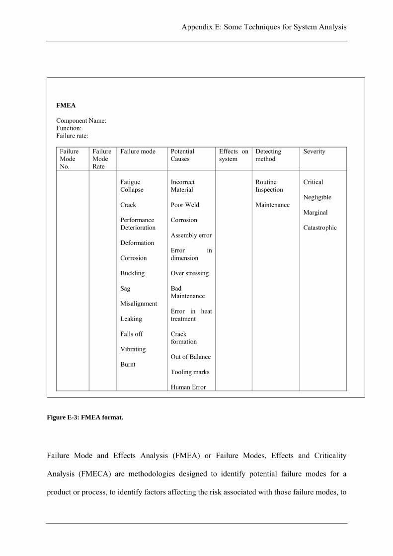
Appendix E: Some Techniques for System Analysis
FMEA Component Name: Function: Failure rate:
Failure Mode No.
Failure Mode Rate
Failure mode Potential Causes
Effects on system
Detecting method
Severity
Fatigue Collapse Crack Performance Deterioration Deformation Corrosion Buckling Sag Misalignment Leaking Falls off Vibrating Burnt
Incorrect Material Poor Weld Corrosion Assembly error Error in dimension Over stressing Bad Maintenance Error in heat treatment Crack formation Out of Balance Tooling marks Human Error
Routine Inspection Maintenance
Critical Negligible Marginal Catastrophic
Figure E-3: FMEA format.
Failure Mode and Effects Analysis (FMEA) or Failure Modes, Effects and Criticality
Analysis (FMECA) are methodologies designed to identify potential failure modes for a
product or process, to identify factors affecting the risk associated with those failure modes, to

Risk Based Life Management of Offshore Structures and Equipment
rank the issues in terms of importance and to identify corrective actions to mitigate the
concerns. The FMEA required the identification of the following basic information:
Components.
Function of each component.
Possible damage mechanisms and locations.
Causes of damage mechanisms.
Consequences of a failure.
Current control.
Possible mitigating actions.
By identifying this information it is then possible to understand what components need to be
considered in a management plan and how they are operated (e.g. environments, loading
conditions). From knowledge of the service conditions it is then possible to identify how the
life of the components may be consumed (What damage mechanisms may act on the
component within the possible identified service conditions). Once we know how a
component could fail it is then possible to look at what may be the consequences if it did
actually fail. By understanding what fails, how it fails, what conditions affect the damage
mechanisms, and what the consequences might be, it is possible to identify ways that these
factors can be managed.
By having this thorough knowledge it is then possible to construct more generic techniques
for assessing the risk of failure by qualitative or quantitative methods.

Appendix F: Qualitative Analysis: The Risk Matrix Approach
APPENDIX F: QUALITATIVE ANALYSIS: THE RISK
MATRIX APPROACH
The risk matrix Approach
This is a common technique for risk analysis in which system components are broadly ranked
(in qualitative terms) depending on their likelihood of failure and the consequence of failure.
An example risk matrix is shown in figure F-1.
VH
Gear Box failureH
Failu re Probability
M T urbine failu re
L
VL
VL L M H VH
C onsequence Severity
Figure F-1: Example of a risk matrix.
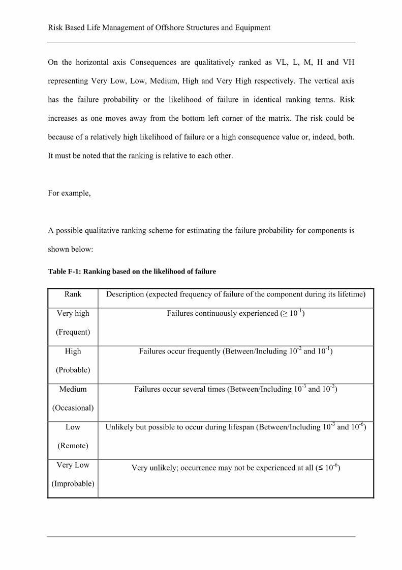
Risk Based Life Management of Offshore Structures and Equipment
On the horizontal axis Consequences are qualitatively ranked as VL, L, M, H and VH
representing Very Low, Low, Medium, High and Very High respectively. The vertical axis
has the failure probability or the likelihood of failure in identical ranking terms. Risk
increases as one moves away from the bottom left corner of the matrix. The risk could be
because of a relatively high likelihood of failure or a high consequence value or, indeed, both.
It must be noted that the ranking is relative to each other.
For example,
A possible qualitative ranking scheme for estimating the failure probability for components is
shown below:
Table F-1: Ranking based on the likelihood of failure
Rank Description (expected frequency of failure of the component during its lifetime)
Very high
(Frequent)
Failures continuously experienced (≥ 10-1)
High
(Probable)
Failures occur frequently (Between/Including 10-2 and 10-1)
Medium
(Occasional)
Failures occur several times (Between/Including 10-3 and 10-2)
Low
(Remote)
Unlikely but possible to occur during lifespan (Between/Including 10-3 and 10-6)
Very Low
(Improbable)
Very unlikely; occurrence may not be experienced at all (≤ 10-6)

Appendix F: Qualitative Analysis: The Risk Matrix Approach
A possible qualitative ranking scheme for estimating the severity of the consequence of
failure of a component within a ship is shown below:
}
Rank Description (expected cost of the consequence of failure)
Very high Failure has a knock down effect on the entire operation thus causing massive
operational loss apart from rectification costs e.g. event involving loss of lives,
Ship, Cargo, and spillage of Cargo causing widespread environmental damage. This
would involve certain intangibles such as reputational loss etc.
High Failure results in a stand-alone loss of operation apart from rectification costs. E.g.
Ship becomes unavailable for sometime and Cargo is damaged
Medium Failure results in Cargo damage and/or pollution
Low Failure results in partial operational loss; damage may be rectified soon- no
substantial loss of operation
Very low Failure results in a very temporary production loss; damage is rectified
The analysis can become semi-quantitative if the Likelihood of Failure or Consequences are
quantified to some extent. An example of how this could be achieved is shown below.
A variant of the above technique can be a ‘risk histogram’ that assigns relative likelihood and
consequence values and normalizes them. The product of these values is then used to get a
risk number (RN) which is the product of normalized likelihood value and normalized
consequence value. RN values are used to construct the risk histogram (figure F-2). The
values for likelihood and consequence can also be then used to construct a risk matrix

Risk Based Life Management of Offshore Structures and Equipment
(figure F-3). It may be noted that the approach here is semi-quantitative and the risk values
used here are relative and not absolute. Also, there may be circumstances where a simple
product between relative likelihood and consequence is not appropriate, particularly when
consequences are high. For example, instead of
CPR
where P= the probability of failure and
C= the consequence of failure,
a measure of risk could be
nCPR
where n is a number that enables risk to be evaluated on a non-linear scale.
Risk matrix and similar techniques are very useful tools to conduct a very preliminary risk
assessment. Expert opinion, and not complex calculations or elaborate historical failure data,
is often the only input that they require. This simplicity is, however, often its weakest point -
the technique does not take the analysis further to determine how failures occur and what
factors could mitigate risk.

Appendix F: Qualitative Analysis: The Risk Matrix Approach
Risk Histogram using Risk Numbers (RN)
0
20
40
60
Elec C
ontro
l
Gear B
ox
Yaw S
yste
m
Entire
Tur
bine
Gener
ator
Hydra
ulic
Grid C
onne
ction
Blades
Brake
s
Axle/ B
earin
g
Mec
h Con
trol
Entire
Nac
elle
Coupli
ng
Tower
Foun
datio
n
Component number
RN
Figure F-2: Example of a using a measure of risk (RN) to highlight critical components
Figure F-3 Risk matrix using Risk Numbers (RN)

Risk Based Life Management of Offshore Structures and Equipment

Appendix G: Wind Turbines
APPENDIX G: WIND TURBINES
G.1 A HISTORICAL PERSPECTIVE
Wind turbines (WT) are rotating machines that convert kinetic energy of the wind into
mechanical energy and then electrical energy. WTs are variously called as wind generator,
wind power unit (WPU) or wind energy converter (WEC). In the current context, the term
wind turbine (WT) is used and is meant to include the structure on which turbines are
mounted. If the mechanical energy is directly used by machinery for functions such as
pumping or grinding, the machine is called a windmill.
Windmills have been used for at least 3000 years for grinding grain or pumping water
(Burton, 2001). From the thirteenth century, horizontal axis windmills were used as an
integral part of the rural economy. The use of wind mills abated with the advent of cheap
fossil-fuelled engines and the spread of rural electrification. The use of wind to generate
electricity can be traced to the late nineteenth century with the 12KW DC windmill generator
(WT) constructed by Brush in the USA. For much of the twentieth century, there was not
much interest in using wind turbines on a large scale for power generation with the notable
exception of the 1250 KW Smith-Putnam wind turbine constructed in the USA in 1941. This
remained the largest wind turbine for about 40 years (Putnam, 1948).
In the early 1970s, the sudden increase in the price of oil spurred renewed interest in wind
energy. Government funding for research, development and demonstration in this area
became easier. The US, the UK, Denmark, Germany and Sweden were particularly more
active in pursuing programmes at developing wind turbines. The price of oil has in recent

Risk Based Life Management of Offshore Structures and Equipment
years again increased and there is a strong belief that alternative forms of energy need to be
developed to reduce the dependence on oil.
Other factors at play are:
Increased awareness regarding the finiteness of earth’s fossil fuel reserves
Increased awareness of the environmental impact of using fossil fuels
Realization about wind as an abundant source of energy
Technological capacity
The vision and the political will to use wind in energy generation
G.2 MODERN DESIGN AND CONSTRUCTION
The principle of operation
A wind turbine is a machine that converts the power in the wind into electricity. As generators
of electricity, wind turbines need to be connected to some electrical network to be
‘transported’ from the point of generation to the point of consumption. Wind turbines these
days usually range from 0.5 MW to 5 MW capacity.
The energy conversion process uses the basic aerodynamic force of lift to produce a net
positive torque on a rotating shaft, resulting in the production of mechanical power at first and
then in its transformation to electricity in a generator. Wind turbines can generate power in
response to wind that is immediately available and it is not possible to store wind the way
Appendix G: Wind Turbines
conventional fuels can be stored. The output of a wind turbine is hence inherently fluctuating.
The most one can do is to limit the output of a wind turbine to a level below what is possible
for the wind to generate. Thus any system to which the wind turbine is connected must be
capable of taking this variability into account.
Wind turbine systems when connected to larger systems serve to reduce electrical load to
conventional generators enabling lesser consumption of conventional fuels. In smaller
systems, there may be some energy storage with backup generators.
Modern wind turbine design
The most common wind turbines these days are the Horizontal Axis Wind Turbine (HAWT)
in which the axis of rotation is parallel to the ground. A further classification is according to
the rotor orientation - upwind or downwind of the tower, hub design (rigid or teetering), rotor
control mechanism (pitch Vs stall, number of blades (usually two or three blades), and how
they are aligned with the (free yaw or active yaw).
Main sub-systems within a Horizontal Axis Wind Turbine (HAWT)
The main components of the HAWT are shown in the figure F-1.
The principal subsystems of a typical horizontal axis wind turbine shown in the figure are:
The rotor that in the current context includes the blades and the supporting hub;
Risk Based Life Management of Offshore Structures and Equipment
The drive train, which includes the rotating parts of the wind turbine (excluding the
rotor). It usually comprises shafts, gearbox, coupling, a mechanical brake, and the
generator;
The nacelle and mainframe, including wind turbine housing, bed plate, and the yaw
system;
The tower and the foundation;
The machine controls;
The balance of the electrical system, including power cables, switchgear protection,
transformers and power converters.
The following variations in wind turbine design can be found:
Number of blades (usually two or three);
Rotor orientation, downwind or upwind of tower;
Blade material, construction method, and profile;
Hub design- rigid, tethering or hinged;
Power control- aerodynamic control (stall control) or variable pitch blades (pitch
control);
Fixed or variable rotor speed;
Orientation by self aligning action (free yaw), or direct control (active yaw);
Synchronous or induction generator;
Gearbox or direct drive generator.

Appendix G: Wind Turbines
Figure G-1: Schematic of a typical horizontal wind turbine
Rot
or
Hub
Control
Drive train Generator
Main frame/ yaw system Bearings…
Tow
er
Foundation
Nacelle Cover
Balance of Electrical System (transformer, Protective switch gear)
Shaft

Risk Based Life Management of Offshore Structures and Equipment
G.3 KEY COMPONENTS
Key Wind Turbine Components include:
(a) Rotor
The rotor consists of the blades and the hub of the wind turbine. These constitute the most
important components within the wind turbine from the point of view of performance as well
as cost. Most wind turbines these days have an upwind rotor with three blades although some
down wind rotors and two blade rotors has been in existence. Single blade turbines have also
been built in the past. Most intermediate sized wind turbines, especially those from Denmark,
have fixed blade pitch and stall control. However, now the emerging trend is towards pitch
control for larger machines. The blades are made of composite material- primarily fibre glass
reinforced plastics, but sometimes wood/ epoxy laminates are also used.
(b) Drive Train
The drive train consists of all the rotating parts of a wind turbine with the exception of the
rotor blades. There is a low speed shaft on the rotor side, a gear box, and a high speed shaft on
the generator side. Other drive train components include the support bearings, one or more
couplings, a brake, and the rotating parts of the generator. The gearbox increases the rate of
rotation of the rotor from a low value, of the order of tens of rpm (rotations per minute), to the
order of hundreds or thousands of rpm as required by the generator to generate electrical
power. Some wind turbines, however, have specially designed generators that can operate at
low speeds thereby obviating the need of a gear box. In WTs in which power is generated at a

Appendix G: Wind Turbines
higher machine rpm (i.e. turbines with gears) there is a low speed shaft leading up to the gear
box, and a high speed shaft between the gear box and the generator.
(c) Generator
The generators take in mechanical power as input to give electrical power as the output. There
are mostly two types of generators in use- induction generators and synchronous generators.
Most of the turbines that are connected to the grid use induction generators. The main
advantage of induction generators are that they are rugged, inexpensive, and easy to connect
to the electrical network. However, an induction generator operates in a narrow band of
speeds at slightly higher than the synchronous speed of the machine.
The synchronous generator offers some advantages over the induction generator- it is a
variable speed machine which can operate in a wider range of wind speeds thus increasing
energy capture. There is a general reduction in the wear and tear of the WT system by using
synchronous generators. However, the generator itself is more complex than the induction
machine requiring more of maintenance attention.
(d) Nacelle and Yaw System
This system includes the wind turbine housing, the machine bedplate or main frame, and the
yaw orientation system. The mainframe provides for the mounting and the proper alignment
of the drive train components and the nacelle cover protects the contents from the weather.
The yaw mechanism aligns the rotor shaft such maximum energy from the wind can be
harvested. The main component here is a large bearing that connects the main frame to the
tower. Upwind wind turbines mainly use an active yaw drive, comprising a number of yaw

Risk Based Life Management of Offshore Structures and Equipment
motors, each of which drives a pinion gear against a bull gear attached to the yaw bearing.
This mechanism is controlled by an automatic yaw control system to which is connected a
sensor to detect the wind direction. The system may also have a brake to hold the nacelle in
the aligned position. Free yaw mechanisms, on the other hand, are commonly used on
downwind wind turbines to self-align rotor with the wind.
(e) Tower and Foundation
This system includes the tower structure and the supporting foundation. There are mainly two
types of towers (1) free standing types using steel tubes, lattice towers, and concrete towers
and (2) guyed towers that are used for smaller turbines. The height of the tower is usually 1 to
1.5 times the rotor diameter, but in any case is normally 20 m (Manwell, J.F.; McGowan,
J.G.; Rogers, A.L.; 2005)
Tower selection is influenced by the characteristics of the site. The stiffness of the tower is a
major factor in wind turbine system dynamics because of the possibility of coupled vibrations
between the rotor and the tower.
(f) The control system
The control system in general includes the following:
Sensors e.g. Anemometer, Wind Vane, Rotor speed Sensor, Electrical power
sensor, Pitch position sensor, vibration sensors, temperature and oil level
indicators, etc.
Appendix G: Wind Turbines
The Controller that is a system of hardware and software processing input signals
from the sensors and generating output signals for the actuators
Actuators included hydraulic or electric pitch actuator, generator contactors,
switches for activating shaft brakes, yaw motors, etc.
The functions of a WT controller can be broadly classified into:
Supervisory control that brings the turbine from one operational state to another
for e.g., stand-by, start-up, stalling, shutdown, stop with a fault.
Closed loop control which is usually a software based feedback mechanism that
adjusts the operational state of the turbine such that it remains within pre-defined
operating parameters
The safety system that brings the system to a safe condition (usually in a state of
rest) to pre-empt failure for e.g., the safety system might be tripped due to rotor
over speed, excessive vibration, and other events such as a lightening strike.
(g) Clutches and Brakes
Clutches transmit torque when applied and do not do so when they are released. Clutches are
typically applied by spring pressure and released through an active mechanical or
electromechanical mechanism. Brakes function to bring a drive train or the yaw mechanism,
for example, to a halt. The main difference between a clutch and a brake is that heating is a
more important factor in a brake than a clutch.

Risk Based Life Management of Offshore Structures and Equipment
G.4 RECENT DEVELOPMENTS IN THE WIND TURBINE SECTOR:
Current drivers for interest in wind farms are mainly the high cost of fossil fuels and the
carbon emissions associated with the use of fossil fuels.
The UK Government’s Third Annual Report released in July 2006 on the implementation of
the Energy White Paper (2003) underlines its policy to cut UK’s carbon emissions by 60% by
the year 2050, with real progress by the year 2020 (DTI, 2002).
A shift from fossil based energy generation, which is responsible for a substantial proportion
of CO2 emission, to the relatively clean energy generated from renewable sources is one of
measures envisaged towards reducing carbon emissions. Wind energy is widely believed to be
an abundant indigenous source of energy in the UK, and it is estimated that much of this
renewable energy shall come from wind farms. Low CO2 emissions over the entire life cycle
of wind turbine (and structure) manufacture, installation, operation and de-commissioning,
have the potential to help limit climate change.
There continues to be progress in a number of areas in wind turbine technology: the rating of
WT generators (in terms of the power output) has increased; there is better condition
monitoring and better protection devices installed; two blade wind turbines are also being re-
considered; factors such as noise pollution, aesthetics and yield have encouraged an
increasing trend in locating Wind Farms offshore; floating Wind Turbines (obviating the need
for foundations in the sea bed) are also being tested.