Risk aversion and the impact of health insurance onhousehold vulnerability: New evidence from rural

Vietnam

Thang Vo∗

Australian National University

May 31, 2016

Abstract

This study provides new evidence on the impact of health insurance coverage

on household vulnerability using Vietnam Access to Resources Household Surveys

(VARHS) during 2010-2012. The outcomes of interest are the probability of falling

into poverty (VEP) and the magnitude of utility loss (VEU). Since the data set

is not from an intervention program, the propensity score- matching method is

employed to construct treatment and control groups. Risk aversion is calculated

and used as an important explanatory variable for health insurance enrollment. The

estimates show that health insurance coverage helps rural households in Vietnam

reduce the idiosyncratic component of utility loss by 81 per cent and has the added

benefit of reducing the probability of being poor by about 19 per cent. The reverse

effect of the risk aversion on health insurance enrollment implies not only a potential

‘rigidity’ effect on health insurance demand but also deficiencies in health insurance

market. The study suggests practical implications for the government to attain its

goal of universal health insurance coverage.

Keywords: health insurance, impact evaluation, vulnerability, risk aversion, VARHS,

Vietnam.

JEL Classification Numbers: R14, H0, XY.

∗Address: 1A Hoang Dieu, Phu Nhuan, Ho Chi Minh City, Vietnam; telephone: +84-934-05-1018;e-mail: thang.vo@anu.edu.au.

1

1 Introduction

One of the worst shocks to households is a serious illness of one of its members. This

has a negative and significant effect on consumption and income. Illness raises two

important economic costs: the cost of medical care and income loss due to reduced

labor supply. The unpredictable nature of these two costs makes households unable

to smooth their consumption over periods of major illness. This is particularly true in

developing countries where few individuals have health insurance. In addition, households

in developing countries find it difficult to access the formal credit market. Therefore, they

have to rely on informal coping mechanisms such as drawing on savings, selling assets,

transfers from other families or social support networks. Low-income households who

cannot use these channels to smooth their consumption are more likely to fall into a

poverty trap. In other words, the burden of health care pushes individuals experiencing

illness into poverty or forces them into deeper poverty.

There are a huge number of studies investigating the impact of health insurance on

health status, health service use or out-of-pocket payment. Scholars have also conducted

several studies that focus on the relationship between health insurance coverage and ex-

post poverty. Recently, some studies have examined the impact of money transfers such

as microfinance and remittance on ex-ante vulnerability. However, there is no study

for any country that measures the impact of health insurance coverage on household

vulnerability. This paper attempts to fill this gap in the empirical literature and in this

case health insurance has been considered as one of the crucial strategies for coping with

vulnerability arising from idiosyncratic shocks. In this sense, this paper is the first to

investigate the role of health insurance in mitigating vulnerability1.

Using the propensity score matching method and data from Vietnam Access to Re-

sources Household Surveys (VARHS) during 2010-2012, we investigate whether having

1“Research into alternative health care financing strategies and related mechanisms for coping withthe direct and indirect costs of illness is urgently required to inform the development of appropriate socialpolicies to improve access to essential health services and break the vicious cycle between illness andpoverty.” (McIntyre et al. 2006)

2

health insurance coverage has any impact on the probability of falling into poverty (VEP)

and the magnitude of utility loss (VEU). In particular, households risk preference has

been taken into account when measuring health insurance demand. Our estimates show

that health insurance helps rural households in Vietnam reduce the idiosyncratic compo-

nent of utility loss by 81 per cent. In addition, health insurance helps rural households

in Vietnam reduce the probability of becoming poor by about 19 per cent. In addition,

the reverse effect of the risk aversion on health insurance enrollment implies not only a

potential ‘rigidity’ effect on health insurance demand but also deficiencies in the health

insurance market. Therefore, the study suggests implications for both demand side and

supply side of the health insurance market so that the government is able to reach its

goal of universal health insurance coverage.

The remainder of the paper is structured as follows. Section 2 reviews studies on

the topic of vulnerability and health insurance impact. Section 3 provides an overview

of health insurance schemes in Vietnam. Section 4 and Section 5 are dedicated to data

description and analytical framework, respectively. Section 6 discusses the results and

the last section concludes the paper.

2 Literature review

Concepts of vulnerability

The concept of vulnerability is interpreted in various ways in different contexts. In

economics, the concept of vulnerability emerges from that of poverty. From the traditional

view of poverty as reflected in World Development Report 1990, the notion of poverty

consists of material deprivation and low achievement in education and health (World

Bank 1990). Later, the term ‘vulnerability’ is mentioned when examining the relationship

between poverty and uncertainty of income (Morduch 1994). Since then, ‘vulnerability’

is often used to extend the traditional concept of poverty. While poverty measurement

is based on fixed standards such as income or expenditure during a short period of time,

3

vulnerability broadens the poverty notion by including the potential risk of adverse shocks

such as income loss, bad health (idiosyncratic risks) and natural disasters (covariate risks).

For example, in the work of Glewwe & Hall (1998) and Cunningham & Maloney (2000),

vulnerability is defined as exposure to negative shocks to welfare. It is also defined as “the

probability or risk today of being in poverty or to fall into deeper poverty in the future”

(World Bank 2001) or “the ex-ante risk that a household will, if currently non-poor, fall

below the poverty line, or if currently poor, will remain in poverty” (Chaudhuri 2003).

In an excellent summary of risk and vulnerability, Hoddinott & Quisumbing (2003)

classify approaches to assessing vulnerability into three methods according to their dis-

tinct definitions: vulnerability as expected poverty (VEP); vulnerability as low expected

utility (VEU); and vulnerability as uninsured exposure to risk (VER). All three methods

predict changes in welfare, but with different welfare measurements. The difference be-

tween VEP and VEU lies in their definitions of welfare: in VEP consumption is regarded

as welfare, while VEU uses utility derived from consumption. While VEP and VEU com-

monly use a benchmark for a welfare indicator (z ) and estimate the probability of falling

below this benchmark (p), VER evaluates whether downside risks or observed shocks

result in welfare loss. In other word, VER assesses the household’s ability to smooth or

insure consumption when faced with income shocks, while maintaining a minimum level

of assets.

Health insurance and household vulnerability

The relationship between health insurance coverage and household vulnerability emerges

from the impact of health shocks on poverty and vulnerability. Illness, a major part

of idiosyncratic shocks, can push non-poor household into poverty, or poor households

into extreme poverty (Calvo & Dercon 2005, Carter et al. 2007, Dercon 2004)2. Accord-

ing to World Bank (2003), illness pushes households into poverty, through lost wages,

2The authors show that a random event (e.g. a flood, a drought, an illness, an unemployment spell)can have a permanent effect for households, pushing them into poverty.

4

high spending for catastrophic illness, and repeated treatment for other illnesses. More-

over, health shocks are not only one of the most sizable, but also one of the least pre-

dictable shocks (Gertler & Gruber 2002)3. Although several empirical studies show that

households are able to fully or partially insure themselves against production shocks and

weather shocks, they are less able to cope with health shocks (Fafchamps & Lund 2003).

With production shocks, households tend to choose less risky activities and with weather

shocks, households try to learn and understand them in order to deal with them to

some extent. However, this is not the case with health shocks which are likely to make

households more vulnerable than other types of shocks (Duflo 2005).

Most studies on health problems and health insurance impact focus on financial loss

and healthcare service usage while other papers measure the impact of health insurance

on household poverty status. For instance, McIntyre et al. (2006) finds that health care

payments place a considerable stress on households in low- and middle- income countries.

The burden of health care payments pushes individuals experiencing illness into poverty

or forces them into deeper poverty.

One of the main strategies adopted by many agricultural families who face high costs

of health care is to sell livestock. Another strategy is using intra-household labor sub-

stitution to compensate for labor lost. Also, inter-household transfers of resources might

take a small role (Sauerborn et al. 1996). Similarly, a study for Russia shows that

chronic diseases resulted in higher levels of household healthcare expenditure in Russia

and productivity losses are significantly attributed to reduced labor supply and reduced

household labor income. The authors find that households in Russia depend on infor-

mal coping mechanisms in the face of chronic diseases, irrespective of insurance cover

3Using a panel data for Indonesia, Gertler & Gruber (2002) demonstrate that major illness inducessignificant economic costs and is associated with a fall in consumption. Similarly, Gertler et al. (2009)prove that micro-financial saving and lending institutions can help Indonesian families smooth consump-tion after a major illness. Moreover, Jalan & Ravallion (1999) observe that wealthier Chinese householdsare better able to insure consumption against income shocks. Studies of Rosenzweig & Wolpin (1993)and Fafchamps et al. (1998) present that sale of stocks can help insure consumption. Empirical resultsacross countries also advocate that households find difficult to cope with all income shocks, especiallythose with low assets (Harrower & Hoddinott 2004, Skoufias & Quisumbing 2005).

5

(Abegunde & Stanciole 2008).

Another piece of research shows that about 25.9 per cent of households in forty low-

and middle-income countries borrow money or sell items to pay for health care. The

health shocks are more severe among the poorest households and in countries with less

health insurance. Healthcare systems in developing countries have been failing to insure

families against the financial risks of seeking health care (Kruk et al. 2009).

Literature on health shocks has proved the importance of health insurance. For exam-

ple, a study for India highlights the fact that community-based health insurance schemes

in India can protect poor households from the unpredictable risk of medical expenses

(Kent 2002). Another study using an Indonesian panel data set suggests that public

insurance or subsidies for medical care may improve household welfare by providing con-

sumption insurance (Gertler & Gruber 2002).

However, there is currently no study investigating the impact of health insurance

on household vulnerability. Some attempts has been made to examine the measure the

impact of microfinance on vulnerability or household consumption over time (Khandker

1998, Morduch 1999, Zaman 1999). A study of Swain & Floro (2012) indicate that

vulnerability of members of the Indian Self Help Group (SHG) is not significantly higher

than in non-SHG members, although the SHG members experience a high incidence

of poverty. Nevertheless, the SHG members for more than one year face significantly

reduced vulnerability. Another study by Puhazhendi & Badatya (2002) suggests that

microfinance allows consumption smoothing and helps households mitigate the negative

effects of shocks.

Health insurance impact in Vietnam

A large number of studies using Vietnam data have been conducted to look at the inci-

dence of out-of-pocket for health care as well as the effects of health insurance on various

types of household spending. For example, Wagstaff & Doorslaer (2003), using the data

set of 1993-1998, find that 80 per cent of health spending in Vietnam was paid out-of-

6

pocket in 1998. The out-of-pocket spending is mainly non-hospital expenditure rather

than inpatient care expenses. This primarily forces poor households to become poorer

rather than leading non-poor households into poverty. Later, Wagstaff (2007) shows that

the incomes of urban households are more vulnerable to health shocks than rural house-

holds. The author suggests that transfers from relatives, friends or neighbors partially

offset income losses and extra medical spending, even among insured households. The

paper also finds that households with a health shock consume less food, but spend more

on items such as housing and electricity.

Nguyen (2010) reviews Vietnam’s policies on health services and provides an assess-

ment of public health facilities and the access of people to health care services in Vietnam.

He finds that the poor and ethnic minorities are more likely to be enrolled in health insur-

ance than other people. Health insurance helps the insured increase health care utilization

and reduces out-of-pocket spending. The density of medical staff is also positively corre-

lated with outpatient health care utilization. However, the quality of health care services

and the access to health care services remain limited in poor, remote and mountainous

areas (Nguyen 2010).

Chaudhuri & Roy (2008) use data drawn from the 199293 and 199798 Vietnam Living

Standard Surveys (VLSS) and the 2002 Vietnam Household and Living Standards Survey

(VHLSS) to estimate the probability that an individual will seek treatment and the

determinants of out-of-pocket payments. They show that the rich are more able to

use health insurance effectively with low out-of-pocket payments than are those with

lower incomes. In contrast, the poor suffer higher out-of-pocket payments and are thus

discouraged from seeking treatments until their ailment become serious. When pro-poor

policies are instituted, the healthcare inequality becomes less serious (Chaudhuri & Roy

2008). Further, the insured patients, especially those at lower income levels, are more

likely to use outpatient facilities and public providers (Jowett et al. 2004).

In a study on how households in Vietnam cope with health care expenses, Kim et al.

(2011) examine a rural commune in Hanoi and show that households of all income levels

7

borrow to finance treatment costs but the poor and near-poor are more heavily dependent.

The likelihood of reducing food consumption to pay for extremely high-cost treatment

versus low-cost treatment increases most for the poor in both inpatient and outpatient

contexts. Decreased funding and increased costs of health care rendered Dai Dong’s

population vulnerable to the consequences of detrimental coping strategies such as debt

and food reduction (Kim et al. 2011).

Thanh et al. (2010) indicate that Vietnam’s health care funds for the poor (HCFP)

significantly reduces the health care expenditure (HCE) as a percentage of total expen-

diture, and increases the use of the local public health care among the poor. However,

the impact of HCFP on the use of the higher levels of public health care and the use

of go-to-pharmacies are not significant (Thanh et al. 2010). Sepehri et al. (2006) use

Vietnam Living Standard Surveys 1993 and 1998 to show that health insurance reduces

out-of-pocket expenditure by around 36 per cent to 45 per cent. Sepehri et al. (2011)

find that insurance reduces out-of-pocket expenditures more for those enrollees using dis-

trict and higher level public health facilities than those using commune health centers.

Compared to the uninsured patients using district hospitals, compulsory and voluntary

insurance schemes reduce out-of-pocket expenditure by 40 per cent and 32 per cent, re-

spectively. However, for contacts at the commune health centers, both the compulsory

health scheme and the voluntary health insurance scheme have little influence on out-

of-pocket spending, while the HCFP reduces out-of-pocket spending by about 15 per

cent.

In summary, the evaluation methods used in these studies are propensity score match-

ing (PSM), double difference and triple difference methods. Authors try to eliminate any

biases in the estimated insurance coefficient arising from the unobservable factors that

are correlated with both insurance status variable and the outcomes of interest. Most

studies find a limited impact of insurance on out-of-pocket payments, with the exception

of Jowett et al. (2003) on a voluntary program in Hai Phong. The differences impact

of health insurance among studies are attributed to differences in methods and target

8

groups and the outcomes of interest. For examples, both Bales et al. (2007) and Wagstaff

(2007) use data from VHLSS 2002 and 2004 to estimate impacts of free health insurance

on the poor. They find a significant positive impact of the program on the reduction of

out-of-pocket health care spending. However, while Wagstaff (2007) finds a positive im-

pact of the health insurance on health care utilization, Bales et al. (2007) does not. This

might be the reason why Wagstaff re-conducted the research using different methods in

2010. This time, the results suggest that the HCFP has had no impact on use of services,

but has substantially reduced out-of-pocket spending (Wagstaff 2010).

Unfortunately, there is no paper measuring the impact of health insurance coverage

on household vulnerability even though there are a number of studies exploring risks

and household responses to risks in Vietnam. These studies include Hasegawa (2010),

Klasen & Waibel (2010), Imai et al. (2011), Wainwright & Newman (2011), Montalbano &

Magrini (2012), and Tuyen (2013). Therefore, this study will contribute to the empirical

literature by filling this gap.

Choice under risk and health insurance demand

According to Phelps (2013), people seem to dislike risk and prefer a less risky situation to

a more risky situation, other things being equal. They are thus risk averse and are willing

to pay for insurance in order to eliminate the chance of really risky losses. Therefore,

a household’s purchase of health insurance in this study is regarded as a choice under

risk and uncertainty, partially reflecting the households risk preference. This section

summarizes the literature on risk preference as the framework for risk aversion measures

used in this study.

Since Bernoulli (1954) provided the foundations for the concepts of expected utility

and risk aversion, individual risk preference has become a fundamental building block of a

huge range of economic theory (Isaac & James 2000). A comprehensive review of choice

under risk theories can be seen in Starmer (2000). In general, they are classified into

two major groups: expected utility theory and non-expected utility theory. Therefore,

9

risk preference or risk aversion which is derived from theory can be estimated in two

different ways. First, the conventional way to estimate risk aversion comes primarily

from an idea of expected utility theory that assumes individuals optimize their preference

function when they make choices among prospects (or uncertain outcomes). The studies

following this concept include Von Neumann & Morgenstern (1944); Friedman & Savage

(1948); and Rothschild & Stiglitz (1970). Among empirical studies are the works of

Pratt (1964) and Arrow (1965), who employed a concave utility function U to derive

formal measures of absolute risk aversion. Second, the prospect theory provides another

framework to calculate risk aversion. This theory assumes that individuals make their

choices by decision heuristics, or rules, under particular conditions. In other words,

problem context is an important determinant of choice-rule selection. Two of the most

widely discussed studies are Kahneman & Tversky (1979) and Tversky & Kahneman

(1992). The studies of Gachter et al. (2010) and Abdellaoui (2000) are two empirical

studies that follow this path.

The relationship between individuals’ risk preference and health insurance demand has

been investigated in Friedman (1974), Bleichrodt & Pinto (2000, 2002) and Barseghyan

et al. (2013)4. In addition, the relationship of risk preference and other aspects of health

choice has been studied in Nightingale & Grant (1988), Nightingale (1988), Richardson

(1994), Bleichrodt & Gafni (1996), Bridges (2003), Picone et al. (2004), Lusk & Coble

(2005), Zhang & Rashad (2008), Andersen et al. (2008), and Einav et al. (2010). These

studies explain why we choose to add a risk aversion index into the probit model for

estimating health insurance coverage.

4The relationship between an individuals’ economic behaviour and risk aversion has been investi-gated in many empirical studies. For example, Bowman et al. (1999), Heidhues & Koszegi (2008) withconsumption behaviour; financial markets (Benartzi & Thaler 1995, Odean 1998, Haigh & List 2005);trade policy (Tovar 2009); labor supply (Camerer et al. 1997, Goette et al. 2004, Fehr et al. 2007).

10

3 Overview of the health insurance system in Viet-

nam

Health insurance system in Vietnam

After 1986, when the government launched economic reforms, the healthcare system in

Vietnam was transformed from a centralized one of free universal access to a user-pay

system. The pharmaceutical industry was also privatized. Out-of-pocket spending on

health care went up rapidly. It reached 71 per cent of health spending (mostly on drugs)

in 1993 and 80 per cent in 1998, creating a huge burden for ill households, especially the

poor (Wagstaff & Lieberman 2009).

In 1993, Vietnam introduced a compulsory health insurance (CHI) program, which

was initially aimed at the formal sector worker. A voluntary health insurance scheme

was later added to cover the self-employed, informal sector employees, and dependents of

CHI members. Later, all employees in the formal sectors were required to enroll, rather

than only those in large institutions.

In the early 2000s, other important changes in health insurance were introduced:

copayments were scrapped and the benefit package made more generous, and the insurer

was permitted to contract with private providers. The health sector was decentralized and

much of the revenue was raised locally. Some hospitals were given greater autonomy. In

2002, the insurance system was reformed. The central government launched the Health

Care Fund for the Poor (HCFP) program, to provide insurance coverage for the poor

and other disadvantaged groups. Later, the government continued to expand coverage

through a decree called Decision 139, which asked local governments to provide free health

care to the poor, ethnic minority households living in the remote areas and households

living in communes officially classified as “special poor”5. However, service provision

5In October 2002, Vietnam’s government introduced a new health care fund program for the poorthrough Decision 139. This decision mandated all provincial governments to provide free health care tothree groups: households defined as poor according to official government poverty standards introducedin November 2000; all households regardless of their own assessed income living in communes covered

11

proved to be poor due to the troublesome application process, limited funds, and lack of

public awareness of the scheme itself. Households still suffered from high out-of-pocket

spending.

In 2008, the government enacted the Health Insurance Law that became effective in

2009. It aimed to achieve universal health insurance coverage. Under the provision of the

Law, children under 6 years old and the near poor became a compulsory group. Later

in 2010, students and pupils (who used to be in the voluntary group) were included.

Moreover, farmers, workers in agriculture, forestry, fisheries, and salt production sectors

were targeted to be included in 2012 (Matsushima & Yamada 2014).

According to JAHR (2013), the household out-of-pocket payment share of total health

spending in Vietnam is much higher than the WHO recommendation (30-40%)6. House-

holds without health insurance cards, households in rural areas and poor households have

lower out-of-pocket spending on health, but higher catastrophic spending and impover-

ishment due to health spending. Since 2010, in Vietnam the out-of-pocket payment share

of total health expenditure and the proportion of population facing catastrophic spending

and impoverishment due to health spending have decreased compared to previous years.

The health insurance share of total health spending and the volume of medical services

reimbursed by insurance have both increased over time. This result can be attributed to

some recent social and health policies especially policies on healthcare for the poor and

children under six years - along with healthcare subsidies for beneficiaries of social welfare

policies, and most recently, the Law on Health Insurance that commenced in 2009.

Vietnam has a goal of universal health insurance, and many policies on health in-

surance have been promulgated and effectively implemented (Somanathan 2014). The

by a program set up as a result of another policy known as Decision 135 dating from 1998, whichprovides support and services to especially disadvantaged communes; and ethnic minorities living in theprovince of Thai Nguyen and the six mountainous provinces designated by Decision 186 as facing specialdifficulties.

6Household out-of-pocket spending on health accounts for from 8.3 to 11.0% of household capacity topay and approximately 4.6 to 6.0% of total household expenditure. There were 3.9 to 5.7% of households,or approximately 1 million households facing catastrophic spending and 2.5 to 4.1% of households, orapproximately 600000 households facing impoverishment due to health spending between 2002 and 2010.

12

government fully subsidizes health insurance premiums for over 27 million beneficiaries

of social assistance policies, including the poor and children under age 6; and it has con-

tinuously expanded entitlements and increased health insurance premium subsidies for

the near poor, pupils and students. Health insurance has also expanded medical care and

rehabilitation service coverage at each level. In 2012, about 59.31 million people were

insured, accounting for 66.8 per cent of the population7. In some mountainous provinces

with a large number of poor and ethnic minorities population coverage was over 75 per

cent. Frequency of use of medical services reimbursed by insurance reached 2.02 visits

per person. There were 15.6 inpatient visits for every 100 people in the population.

The health insurance fund has become an important funding source for health care. In

2012, the health insurance fund reimbursed facilities for medical services worth approxi-

mately 33,419 billion VND (1.7 billion USD). The health insurance fund has contributed

to strengthening and upgrading the health service delivery network, the range of phar-

maceuticals and technical services available at medical facilities to better meet people’s

demand for health care.

Health Insurance schemes

Currently, Vietnam has two insurance schemes: a compulsory health insurance and a

voluntary scheme. The compulsory scheme initially included two groups: (a) formal

workers (both state and private sectors) and civil servants; and (b) retirees, dependents

of military and police officers, members of Parliament, Communist Party officials, war

heroes, and meritorious people. This scheme later included children younger than 6

years, and from 2003, also covered the poor, ethnic minority households living in the

remote areas, and households living in communes officially classified as “special poor”.

Since 2010, students in schools, colleges and universities, who used to be in the voluntary

insurance group, have also been included. From 2012, the near poor, farmers, workers

in the sectors of agriculture, forestry, fisheries, and salt producers have been targeted for

7The uninsured are mainly the near poor and residents of the rural areas

13

inclusion. Voluntary health insurance is intended for the remaining population.

Since 1992, the health insurance coverage rate has increased considerably. In 1993,

only 5.4 per cent of the total population were covered. The figure in 2010 was around

60 per cent, but by 2012, the figure had grown to 66.8 per cent. Around 60 per cent of

the insured have been completely or partially financed by the state budget (Matsushima

& Yamada 2014, JAHR 2013). However, as can be seen in Table 1, Vietnam health

insurance policies faced difficulties in reaching those non-poor workers and their families

in the informal sector, who belong to the voluntary group. Using the statistics in 2010,

the enrollment rate was only 53.4 per cent for the private enterprises. While most of the

poor and the recipients of social allowance were covered, about 20 per cent of children

under 6 years old remained uninsured despite the fact that their enrolment costs were

fully paid by the state budget. Similarly, the enrollment rate for the near poor was

just 11.38 per cent, although this targeted group was eligible for at least 50 per cent

of subsidies from the government. More importantly, the coverage for the unemployed

remained zero. Therefore, there were still many vulnerable people left without health

insurance (Matsushima & Yamada 2014).

Health insurance premiums and subsidies

According to the Health Insurance Law 2008, the contribution rate for most groups is 4.5

per cent8 of the monthly minimum salary9 or the monthly contract salary depending on

their sources of income (Matsushima & Yamada 2014). In 2010, the premium was about

380,000 VND per person per year. The government subsidized 100 per cent of premiums

for the very poor and for children under 6 years of age, and subsidizes at least 50 per cent

of the premium for the near poor and at least 30 per cent of premiums for students. For

the formal sector workers, employers contributed 3 per cent of the minimum salary and

8In the period 1992-2009, this figure is 3% (Tien et al. 2011)9The minimum salary is determined by the government and serves as a reference for many other

calculation, especially payments from the state budget. In 2009, the minimum salary level is equivalentto US$ 35. In case of health insurance, minimum salary is used to calculate the premium of the poor,the near poor, children under 6, the meritorious people, students

14

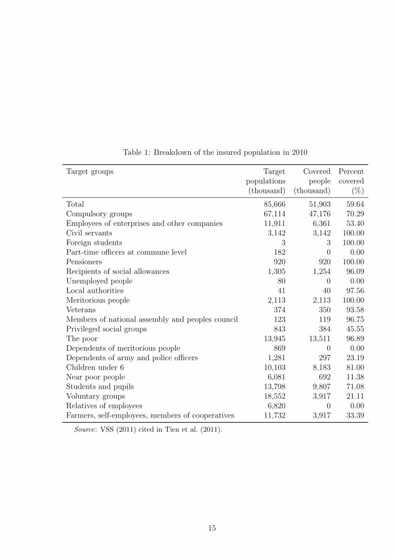
Table 1: Breakdown of the insured population in 2010

Target groups Target Covered Percentpopulations people covered(thousand) (thousand) (%)

Total 85,666 51,903 59.64Compulsory groups 67,114 47,176 70.29Employees of enterprises and other companies 11,911 6,361 53.40Civil servants 3,142 3,142 100.00Foreign students 3 3 100.00Part-time officers at commune level 182 0 0.00Pensioners 920 920 100.00Recipients of social allowances 1,305 1,254 96.09Unemployed people 80 0 0.00Local authorities 41 40 97.56Meritorious people 2,113 2,113 100.00Veterans 374 350 93.58Members of national assembly and peoples council 123 119 96.75Privileged social groups 843 384 45.55The poor 13,945 13,511 96.89Dependents of meritorious people 869 0 0.00Dependents of army and police officers 1,281 297 23.19Children under 6 10,103 8,183 81.00Near poor people 6,081 692 11.38Students and pupils 13,798 9,807 71.08Voluntary groups 18,552 3,917 21.11Relatives of employees 6,820 0 0.00Farmers, self-employees, members of cooperatives 11,732 3,917 33.39

Source: VSS (2011) cited in Tien et al. (2011).

15

the employees paid 1.5 per cent. The voluntary group paid 4.5 per cent of the minimum

salary but the premium rate could reduce to 3 per cent of the minimum salary if the

enrollees were dependents of salaried workers or civil servants (Tien et al. 2011)10.

Benefits

The insurance is effective when the insured are provided with medical care at the

community health center or district hospital where they are registered, or at higher-level

health facilities to which they are have been referred. Patients can choose to register

for the community health center or district hospital they wish to be treated within the

given options by the government (JAHR 2009). If the insured prefer to be treated in

other commune health centers or district level hospitals, they must then pay the hospital

directly, and the out-of-pocket will be reimbursed later at their place of residence, except

in emergency cases. In the case of an emergency, the treatment will be given for free. The

insured can also use private clinics and receive limited benefit from the health insurance

scheme.

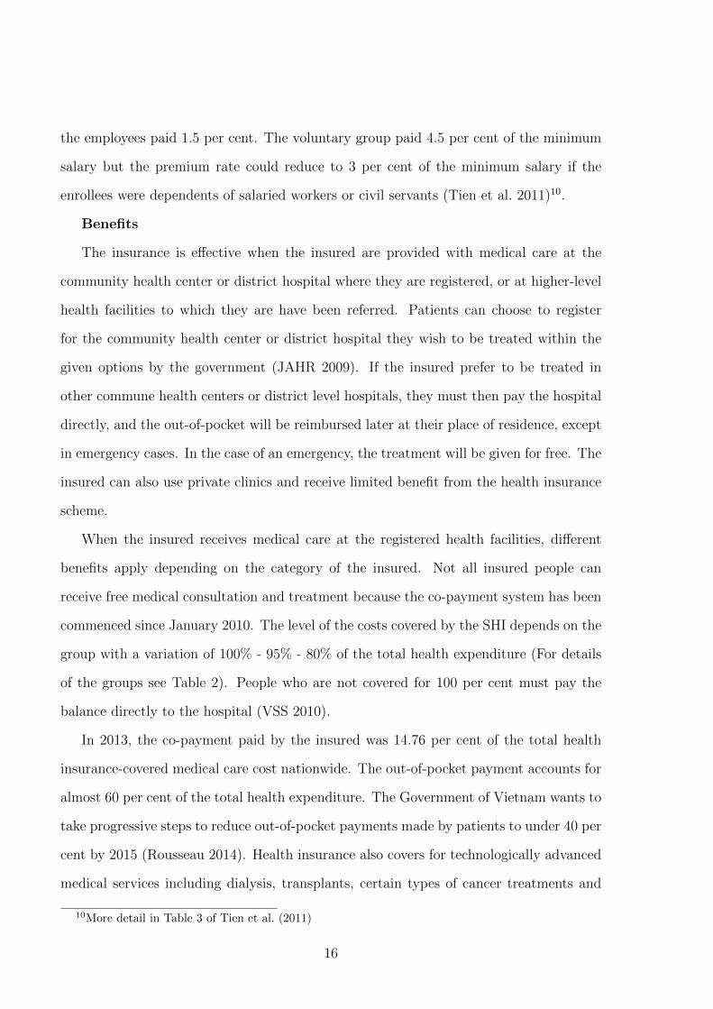
When the insured receives medical care at the registered health facilities, different

benefits apply depending on the category of the insured. Not all insured people can

receive free medical consultation and treatment because the co-payment system has been

commenced since January 2010. The level of the costs covered by the SHI depends on the

group with a variation of 100% - 95% - 80% of the total health expenditure (For details

of the groups see Table 2). People who are not covered for 100 per cent must pay the

balance directly to the hospital (VSS 2010).

In 2013, the co-payment paid by the insured was 14.76 per cent of the total health

insurance-covered medical care cost nationwide. The out-of-pocket payment accounts for

almost 60 per cent of the total health expenditure. The Government of Vietnam wants to

take progressive steps to reduce out-of-pocket payments made by patients to under 40 per

cent by 2015 (Rousseau 2014). Health insurance also covers for technologically advanced

medical services including dialysis, transplants, certain types of cancer treatments and

10More detail in Table 3 of Tien et al. (2011)

16

Table 2: Benefits for basic medical services

100% medical consultation and 95% of medical consultation and 80% oftreatment costs treatment costs the cost

– Specialized technical officers – Persons on pension or monthly – Other– Specialized technical working capacity loss allowance categories

non-commissioned officers – People on monthly social welfare of the– Professional officers allowance as prescribed by law insured– Professional non-commissioned – Poor household members, ethnic

officers of the People’s Public minorities living in areas withsecurity difficult or exceptionally difficult

– Meritorious persons socio-economic conditions– Children under 6 – Other categories of the insured

Source: VSS (2010) cited in Matsushima & Yamada (2014).

cardiovascular operations etc. However, there is a ceiling which is defined as 40 months

of minimum salary (VSS 2010, Tien et al. 2011). In 2012, the minimum salary is between

VND 1.4 million to 2 million depending on residential area. The ceiling is equivalent to

US$ 2,682.8 to US$ 3,838.8 (US$=VND 20,865.50) and therefore the technologically ad-

vanced treatment could result in extremely high out-of-pocket expenditure (Matsushima

& Yamada 2014).

Providers

Health care providers are both public and non-public. Prior to November 2011, all

public providers were automatically approved to participate in social health insurance,

while private providers needed certification and permission. The private sector has grown

steadily during the recent years, but mainly provides outpatient health services and is

still much smaller than the public sector, especially for inpatient treatment (World Health

Organization, 2009)11. In 2014, Vietnam Social Security (VSS) contracted with 1,627

public establishments and 484 private ones (Rousseau 2014). As a result, the proportion

11There has been significant growth in the number of private hospitals in Vietnam since the Govern-ment of Vietnam allowed private investment in the health sector. The number of private hospitals morethan doubled between 2004 and 2008 to reach 82 by 2008. However, this number constituted only 7%of total hospitals, and 4.4% of total hospital beds. Private hospitals were located mainly in urban andwealthy areas (Hort 2011)

17

using private health care services is much higher for the uninsured than the insured.

According to the 2006 VHLSS, the proportion of the number of outpatient contacts in

private health establishment to the total number of outpatient contacts was 23 per cent

for people having voluntary health insurance. The figure for the uninsured people was 43

per cent. Because inpatient treatments are mainly provided by the public health sector,

the proportion of private inpatient contacts to the total inpatient contacts was only 1.2%

and 3.6% for the insured and uninsured people, respectively (Nguyen 2012).

4 Data

Vietnam Access to Resources Household Surveys (VARHS)

Data for this empirical analysis is extracted from two waves of Vietnam Access to Re-

sources Household Survey (VARHS) implemented in 2010 and 2012. The VARHSs are

longitudinal datasets that have been biannually conducted by the University of Copen-

hagen (Denmark) in collaboration with the Centre Institute of Economic Management

(CIEM), the Institute for Labor Studies and Social Affairs (ILSSA), and the Institute of

Policy and Strategy for Agriculture and Rural Development (IPSARD).

These surveys were carried out in rural areas of 12 provinces12 of Vietnam in the

summer of each year, producing a balanced panel of 2,045 households spread over 161

districts and 456 communes. They all were conducted during the same three-month period

each year to ensure consistency and facilitate reasonable comparisons across time. The

VARHS investigates issues surrounding Vietnamese rural household’s access to resources

and the constraints that these households face in managing their livelihoods. Along with

detailed demographic information on household members, the surveys include sections

12They are evenly distributed throughout Vietnam, in seven out of eight regions, with Ha Tay inRed River Delta; Lao Cai and Phu Tho in Northeast; Lai Chau and Dien Bien in Northwest; NgheAn in North Central Coast; Quang Nam and Khanh Hoa in South Central Coast; Dac Lac, Dac Nongand Lam Dong in Central Highland; and Long An in Mekong River Delta. Therefore, these provincescan represent the regional climate and geography throughout the country. However, The sample isstatistically representative at the provincial but not at the national level (Markussen et al. 2012).

18

on household assets, savings, credit (both formal and informal), formal insurance, shocks

and risk-coping, informal safety nets and the structure of social capital (Wainwright &

Newman 2011). There is also a variety of information on communes where households

lived at the time they were surveyed.

Health insurance

In Section 9 of the VARHS questionnaires, there are questions about all the types of

insurance that a household held at the time of interview. They include health insurance

(voluntary and compulsory for labor13), free health insurance for the poor and free health

insurance for children under 6 year old. Other types of insurance consist farmer insur-

ance, fire insurance, life insurance, social insurance, unemployment insurance, education

insurance and vehicle insurance. In this study, we focus on the impact of health insur-

ance in general (both voluntary and compulsory for labor) which is essential for universal

health insurance policy in Vietnam. However, other types of insurance are mentioned in

the later discussion on the impact of risk attitude on health insurance demand.

Risk attitudes

In VARHS 2010 and 2012, there are three questions that enable the derivation of risk

aversion for each individual. The first question is a simple unpaid lottery experiment in

which respondents are required to accept or to reject each of six lotteries with different

payoffs. In each lottery, the winning prize is unchanged at VND 6,000 and the loss varies

from VND 2,000 to VND 7,000 (Table 3).

That exact question in the questionnaire is:

“You are given the opportunities of playing a game where you have a 50:50 chance

of winning or losing (for example, a coin is tossed so that you have an equal chance

of it turning up either heads or tails). In each case choose whether you would accept

or reject the option of playing:”

The VARHS dataset in 2010 and 2012 also contain information that we can use to estimate

13There is no way to separate these two types of health insurance.

19

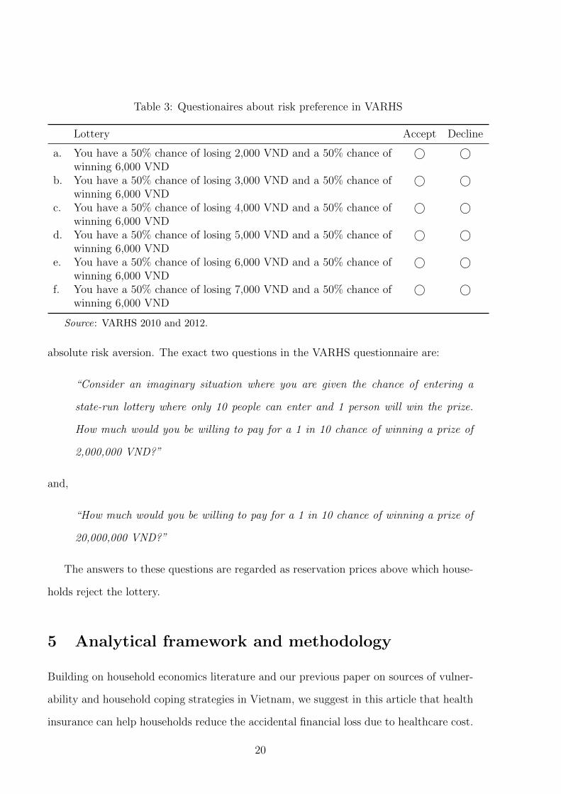
Table 3: Questionaires about risk preference in VARHS

Lottery Accept Decline

a. You have a 50% chance of losing 2,000 VND and a 50% chance of © ©winning 6,000 VND

b. You have a 50% chance of losing 3,000 VND and a 50% chance of © ©winning 6,000 VND

c. You have a 50% chance of losing 4,000 VND and a 50% chance of © ©winning 6,000 VND

d. You have a 50% chance of losing 5,000 VND and a 50% chance of © ©winning 6,000 VND

e. You have a 50% chance of losing 6,000 VND and a 50% chance of © ©winning 6,000 VND

f. You have a 50% chance of losing 7,000 VND and a 50% chance of © ©winning 6,000 VND

Source: VARHS 2010 and 2012.

absolute risk aversion. The exact two questions in the VARHS questionnaire are:

“Consider an imaginary situation where you are given the chance of entering a

state-run lottery where only 10 people can enter and 1 person will win the prize.

How much would you be willing to pay for a 1 in 10 chance of winning a prize of

2,000,000 VND?”

and,

“How much would you be willing to pay for a 1 in 10 chance of winning a prize of

20,000,000 VND?”

The answers to these questions are regarded as reservation prices above which house-

holds reject the lottery.

5 Analytical framework and methodology

Building on household economics literature and our previous paper on sources of vulner-

ability and household coping strategies in Vietnam, we suggest in this article that health

insurance can help households reduce the accidental financial loss due to healthcare cost.

20

Households therefore do not have to reduce consumption as an inevitable coping strategy.

In addition, health insurance reduces the probability of selling productive assets that are

necessary to generate future household income. As well, household members do not have

to suffer their illness without medical treatment due to their difficult financial situation14.

This section describes how we measure vulnerability, risk aversion and finally estimate

the impact of health insurance and risk aversion on vulnerability.

Vulnerability as Expected Poverty (VEP)

Vulnerability as expected poverty is a vulnerability measure which was first proposed and

applied to Indonesian household data by Chaudhuri (2003). This household vulnerability

is defined as the likelihood that a household will fall into poverty in the next period.

VEP can be estimated through the following procedures, beginning with the consumption

function:

lnci = α + βXi + ei (1)

where ci is per capita consumption expenditure for household i, Xi reprerents a vector of

observable household characteristics and commune characteristics (e.g. characteristics of

head, location, assets, prices, shocks), β is a vector of parameters to be estimated, and ei

is a mean-zero disturbance term that captures idiosyncratic shocks that lead to different

levels of per capita consumption.

The variance of the disturbance term is:

σ2e,i = θXi (2)

Chaudhuri et al. (2002) and Chaudhuri (2003) acknowledge that the error term (ei) is

not the same for all households (heteroskedasticity). Therefore, we adopt the three-step

Feasible Generalized Least Squares (FGLS) technique proposed by Amemiya (1977).

14We consider if health insurance affects both idiosyncratic and covariate shocks. Zimmerman &Carter (2003), Morduch (2004) and Dercon (2005) show that the impact of microfinance on the latter islikely to be weak.

21

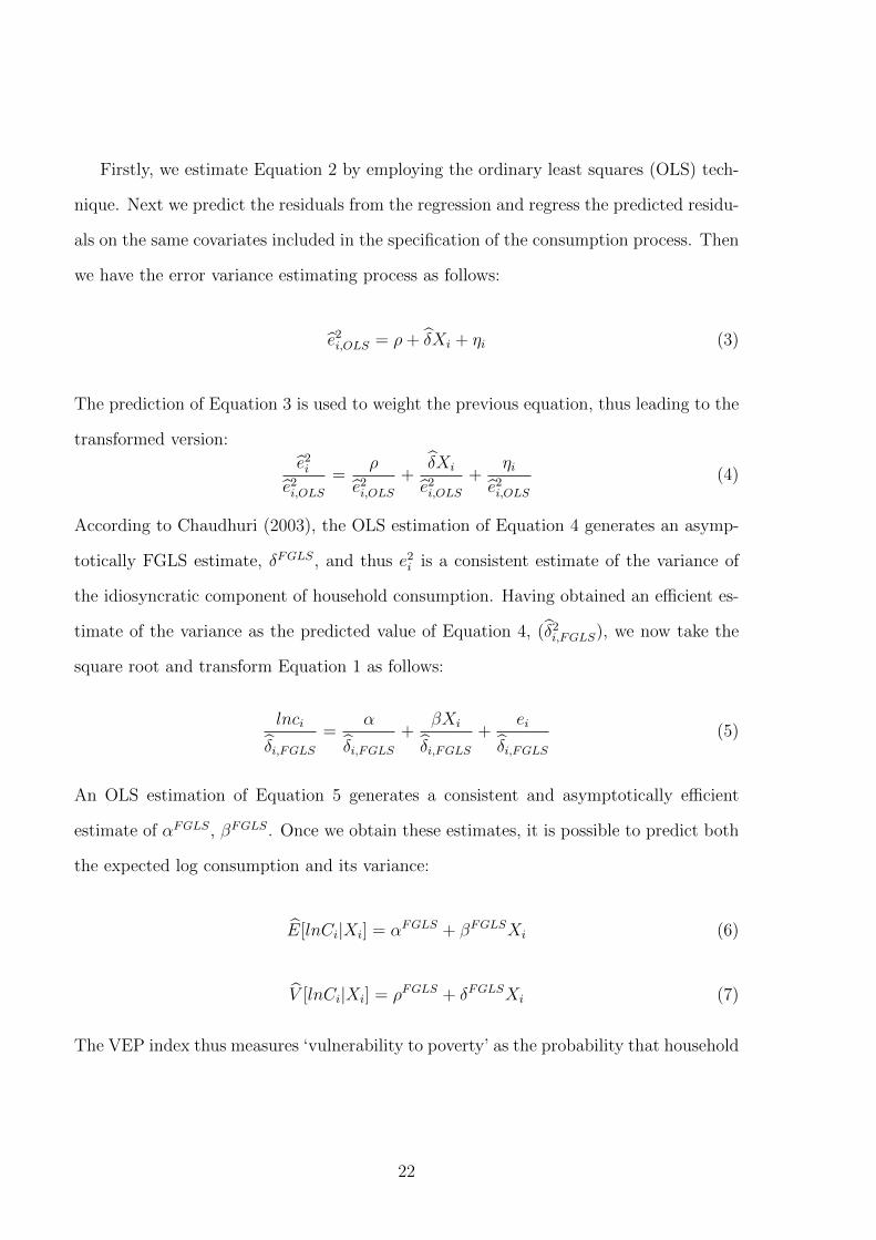
Firstly, we estimate Equation 2 by employing the ordinary least squares (OLS) tech-

nique. Next we predict the residuals from the regression and regress the predicted residu-

als on the same covariates included in the specification of the consumption process. Then

we have the error variance estimating process as follows:

e2i,OLS = ρ+ δXi + ηi (3)

The prediction of Equation 3 is used to weight the previous equation, thus leading to the

transformed version:

e2ie2i,OLS

=ρ

e2i,OLS+

δXi

e2i,OLS+

ηie2i,OLS

(4)

According to Chaudhuri (2003), the OLS estimation of Equation 4 generates an asymp-

totically FGLS estimate, δFGLS, and thus e2i is a consistent estimate of the variance of

the idiosyncratic component of household consumption. Having obtained an efficient es-

timate of the variance as the predicted value of Equation 4, (δ2i,FGLS), we now take the

square root and transform Equation 1 as follows:

lnci

δi,FGLS=

α

δi,FGLS+

βXi

δi,FGLS+

ei

δi,FGLS(5)

An OLS estimation of Equation 5 generates a consistent and asymptotically efficient

estimate of αFGLS, βFGLS. Once we obtain these estimates, it is possible to predict both

the expected log consumption and its variance:

E[lnCi|Xi] = αFGLS + βFGLSXi (6)

V [lnCi|Xi] = ρFGLS + δFGLSXi (7)

The VEP index thus measures ‘vulnerability to poverty’ as the probability that household

22

i will be poor, as follows:

vi,Chaudhuri = P r(lnci < lnz|Xi) = Φ

lnz − E[lnCi|Xi]√V [lnCi|Xi]

(8)

Vulnerability as low Expected Utility (VEU)

Ligon & Schechter (2003) define vulnerability as the variation between the utility derived

from a certainty-equivalent consumption (zce) at and above which the household would

not be considered vulnerable and the expected utility of consumption. This certainty-

equivalent consumption is similar to the poverty line. Consumption of household (ci) has

a distribution that illustrates different states of the world, so the form of vulnerability

measure is given below:

Vi = Ui(zce)− EUi(ci) (9)

where Ui is a weakly concave, strictly increasing function. The equation can be rewritten

as:

Vi = [Ui(zce)− Ui(Eci)] + [Ui(Eci)− EUi(ci)] (10)

The first bracketed term is the variation between utility at zce and utility at expected

consumption (ci) of household i. The second term captures the risk (both covariate and

idiosyncratic risks) faced by household i. It can be decomposed as shown below:

Vi = [Ui(zce)− Ui(Eci)] [Poverty or inequality]

+[Ui(Eci)− EUi(E(ci|xt))] [Covariate or aggregate risk]

+[EUi(E(ci|xt))− EUi(ci)] [Idiosyncratic risk]

(11)

where E(ci|xt) is the commune expected value of consumption, conditional on a vector of

covariant variables (xt).

The authors disintegrate unexplained risk and measurement error out of idiosyncratic

risk and assume that the poverty line (z) is the mean consumption. So Equation 11 can

23

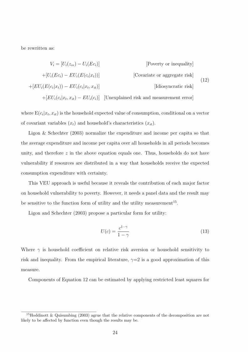
be rewritten as:

Vi = [Ui(zce)− Ui(Eci)] [Poverty or inequality]

+[Ui(Eci)− EUi(E(ci|xt))] [Covariate or aggregate risk]

+[EUi(E(ci|xt))− EUi(ci|xt, xit)] [Idiosyncratic risk]

+[EUi(ci|xt, xit)− EUi(ci)] [Unexplained risk and measurement error]

(12)

where E(ci|xt, xit) is the household expected value of consumption, conditional on a vector

of covariant variables (xt) and household’s characteristics (xit).

Ligon & Schechter (2003) normalize the expenditure and income per capita so that

the average expenditure and income per capita over all households in all periods becomes

unity, and therefore z in the above equation equals one. Thus, households do not have

vulnerability if resources are distributed in a way that households receive the expected

consumption expenditure with certainty.

This VEU approach is useful because it reveals the contribution of each major factor

on household vulnerability to poverty. However, it needs a panel data and the result may

be sensitive to the function form of utility and the utility measurement15.

Ligon and Schechter (2003) propose a particular form for utility:

U(c) =c1−γ

1− γ(13)

Where γ is household coefficient on relative risk aversion or household sensitivity to

risk and inequality. From the empirical literature, γ=2 is a good approximation of this

measure.

Components of Equation 12 can be estimated by applying restricted least squares for

15Hoddinott & Quisumbing (2003) agrue that the relative components of the decomposition are notlikely to be affected by function even though the results may be.

24

expected consumption and then substituting each of them into utility function 13:

Ecit =1

T

T∑t=1

cit (14)

E(cit|Xt) = αi + ηt (15)

E(cit|Xt, Xit) = αi + ηt + βXit (16)

where αi capture the effect of household fixed characteristics; ηt capture the impact of

changes in covariates or aggregates which are the same across households; and β reflects

effects of household characteristics or other observable factors on consumption.

In Equation 16, the income variable may be endogenous if it is treated as an explana-

tory variable for consumption because there may be a feedback relationship between in-

come and consumption. Therefore, we employ the instrumental variable (IV) estimation

for Equation 16 in which income is perceived as an endogenous variable.

Risk aversion calculation

Three questions in the VARHS data enable us to measure individual risk aversion in two

ways. The observed choices of individuals in the lottery enables us to classify respondents

with regard to their level of risk aversion.

First, we derive individual risk aversion from the lottery choice by applying the cu-

mulative prospect theory of Tversky & Kahneman (1992). According to these authors,

individuals will be indifferent between accepting and rejecting the lottery if:

w+(0.5).v(G) = w−(0.5)λriskv(L) (17)

where G is the gain and L is the loss in a given lottery; v(x) is the utility of the outcome

x ∈ [G,L], λrisk is the coefficient of risk aversion in the choice task; w+(0.5) and w−(0.5)

represent the probability weights for the 0.5 chance of gaining G or losing L, respectively

25

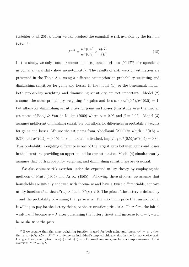
(Gachter et al. 2010). Then we can produce the cumulative risk aversion by the formula

below16:

λrisk =w+(0.5)

w−(0.5)× v(G)

v(L)(18)

In this study, we only consider monotonic acceptance decisions (99.47% of respondents

in our analytical data show monotonicity). The results of risk aversion estimation are

presented in the Table A.4, using a different assumption on probability weighting and

diminishing sensitives for gains and losses. In the model (1), or the benchmark model,

both probability weighting and diminishing sensitivity are not important. Model (2)

assumes the same probability weighting for gains and losses, or w+(0.5)/w−(0.5) = 1,

but allows for diminishing sensitivities for gains and losses (this study uses the median

estimates of Booij & Van de Kuilen (2009) where α = 0.95 and β = 0.92). Model (3)

assumes indifferent diminishing sensitivity but allows for differences in probability weights

for gains and losses. We use the estimates from Abdellaoui (2000) in which w+(0.5) =

0.394 and w−(0.5) = 0.456 for the median individual, implying w+(0.5)/w−(0.5) = 0.86.

This probability weighting difference is one of the largest gaps between gains and losses

in the literature, providing an upper bound for our estimation. Model (4) simultaneously

assumes that both probability weighting and diminishing sensitivities are essential.

We also estimate risk aversion under the expected utility theory by employing the

methods of Pratt (1964) and Arrow (1965). Following these studies, we assume that

households are initially endowed with income w and have a twice differentiable, concave

utility function U so that U ′(w) > 0 and U”(w) < 0. The prize of the lottery is defined by

z and the probability of winning that prize is α. The maximum price that an individual

is willing to pay for the lottery ticket, or the reservation price, is λ. Therefore, the initial

wealth will become w− λ after purchasing the lottery ticket and increase to w− λ+ z if

he or she wins the prize.

16If we assume that the same weighting function is used for both gains and losses, w+ = w−, thenthe ratio v(G)/v(L) = λrisk will define an individual’s implied risk aversion in the lottery choice task.Using a linear assumption on v(x) that v(x) = x for small amounts, we have a simple measure of riskaversion: λrisk = G/L.

26

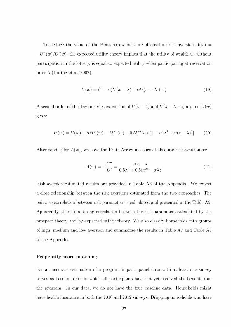
To deduce the value of the Pratt-Arrow measure of absolute risk aversion A(w) =

−U”(w)/U ′(w), the expected utility theory implies that the utility of wealth w, without

participation in the lottery, is equal to expected utility when participating at reservation

price λ (Hartog et al. 2002):

U(w) = (1− α)U(w − λ) + αU(w − λ+ z) (19)

A second order of the Taylor series expansion of U(w−λ) and U(w−λ+z) around U(w)

gives:

U(w) = U(w) + αzU ′(w)− λU ′′(w) + 0.5U ′′(w)[(1− α)λ2 + α(z − λ)2] (20)

After solving for A(w), we have the Pratt-Arrow measure of absolute risk aversion as:

A(w) = −U′′

U ′=

αz − λ0.5λ2 + 0.5αz2 − αλz

(21)

Risk aversion estimated results are provided in Table A6 of the Appendix. We expect

a close relationship between the risk aversions estimated from the two approaches. The

pairwise correlation between risk parameters is calculated and presented in the Table A9.

Apparently, there is a strong correlation between the risk parameters calculated by the

prospect theory and by expected utility theory. We also classify households into groups

of high, medium and low aversion and summarize the results in Table A7 and Table A8

of the Appendix.

Propensity score matching

For an accurate estimation of a program impact, panel data with at least one survey

serves as baseline data in which all participants have not yet received the benefit from

the program. In our data, we do not have the true baseline data. Households might

have health insurance in both the 2010 and 2012 surveys. Dropping households who have

27

health insurance in 2010 then applying the difference-in-difference method to estimate

the average treatment effect on the treated (ATT ) for the year 2012 would lead to a

biased estimate. Therefore, we employ the method of propensity score matching which

has been previously applied by Nguyen (2012).

Let denotes H2010 and H2012 as the binary variables of health insurance in the years

2010 and 2012 respectively. In 2010, Y 20101 and Y 2010

0 denote potential outcomes with

and without health insurance, respectively. Similarly, in 2012, Y 20121 and Y 2012

0 denote

outcomes with and without health insurance.

The impact of health insurance on vulnerability can be presented as below:

ATT2012 = E(Y 20121 |H2012 = 1)− E(Y 2012

0 |H2012 = 1) (22)

The equation can be rewritten as:

ATT2012 = Pr(H2010 = 1|H2012 = 1)ATT2012a + Pr(H2010 = 0|H2012 = 1)ATT2012b (23)

where Pr(H2010 = 1|H2012 = 1) and Pr(H2010 = 0|H2012 = 1) are the proportion of

households with and without health insurance in 2010 among households who have health

insurance in 2012. The ATT2012a and ATT2012b are defined as follows:

ATT2012a = E(Y 20121 |H2012 = 1, H2010 = 1)− E(Y 2012

0 |H2012 = 1, H2010 = 1) (24)

ATT2012b = E(Y 20121 |H2012 = 1, H2010 = 0)− E(Y 2012

0 |H2012 = 1, H2010 = 0) (25)

Here ATT2012a is the average effect of health insurance on people who have health in-

surance in both 2010 and 2012, whereas ATT2012b represents the average effect of health

insurance on the newly insured households in 2012. ATT2012a and ATT2012b will be equal

to ATT2012 under an assumption that the enrolment in health insurance in 2010 is not

correlated with the enrolment in health insurance in 2012. If the assumption does not

28

hold, we need to make other assumption to identify ATT2012.

First, we can write ATT2012 conditional on X as follow:

ATT2012,X = Pr(H2010 = 1|X,H2012 = 1)[E(Y 20121 |X,H2012 = 1, H2010 = 1)

− E(Y 20120 |X,H2012 = 1, H2010 = 1)]

+ Pr(H2010 = 0|X,H2012 = 1)[E(Y 20121 |X,H2012 = 1, H2010 = 0)

− E(Y 20120 |X,H2012 = 1, H2010 = 0)]

(26)

ATT2012,X can be seen as the weighted average of the impact of health insurance on

the newly insured households in 2012 and the impact of health insurance on the insured

households in both 2010 and 2012 (conditional on X)

We suggest two identification assumptions as follows:

E(Y 20120 |X,H2010 = 0, H2012 = 1)− E(Y 2012

0 |X,H2010 = 0, H2012 = 0)

= E(Y 20100 |X,H2010 = 0, H2012 = 1)− E(Y 2010

0 |X,H2010 = 0, H2012 = 0)

(27)

E(Y 20120 |X,H2010 = 1, H2012 = 1)− E(Y 2010

1 |X,H2010 = 1, H2012 = 1)

= E(Y 20120 |X,H2010 = 1, H2012 = 0)− E(Y 2010

1 |X,H2010 = 1, H2012 = 0)

(28)

The first assumption shows that difference in the non-health-insurance outcome (condi-

tional on X) between households uninsured in both the years and those insured only

in the year 2012 is constant overtime. The second assumption indicates that difference

between the non-health-insurance outcome in the year 2012 and the health-insurance out-

come in the year 2010 is the same for households insured in both ears and those insured

in 2010 but not in 2012.

29

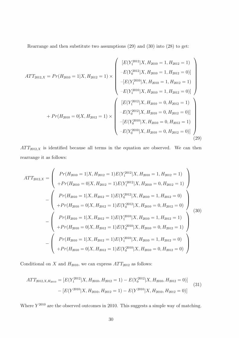
Rearrange and then substitute two assumptions (29) and (30) into (28) to get:

ATT2012,X = Pr(H2010 = 1|X,H2012 = 1)×

[E(Y 20121 |X,H2010 = 1, H2012 = 1)

–E(Y 20120 |X,H2010 = 1, H2012 = 0)]

–[E(Y 20101 |X,H2010 = 1, H2012 = 1)

–E(Y 20101 |X,H2010 = 1, H2012 = 0)]

+ Pr(H2010 = 0|X,H2012 = 1)×

[E(Y 20121 |X,H2010 = 0, H2012 = 1)

–E(Y 20120 |X,H2010 = 0, H2012 = 0)]

–[E(Y 20100 |X,H2010 = 0, H2012 = 1)

–E(Y 20100 |X,H2010 = 0, H2012 = 0)]

(29)

ATT2012,X is identified because all terms in the equation are observed. We can then

rearrange it as follows:

ATT2012,X =

Pr(H2010 = 1|X,H2012 = 1)E(Y 20121 |X,H2010 = 1, H2012 = 1)

+Pr(H2010 = 0|X,H2012 = 1)E(Y 20121 |X,H2010 = 0, H2012 = 1)

−

Pr(H2010 = 1|X,H2012 = 1)E(Y 20120 |X,H2010 = 1, H2012 = 0)

+Pr(H2010 = 0|X,H2012 = 1)E(Y 20120 |X,H2010 = 0, H2012 = 0)

−

Pr(H2010 = 1|X,H2012 = 1)E(Y 20101 |X,H2010 = 1, H2012 = 1)

+Pr(H2010 = 0|X,H2012 = 1)E(Y 20100 |X,H2010 = 0, H2012 = 1)

−

Pr(H2010 = 1|X,H2012 = 1)E(Y 20101 |X,H2010 = 1, H2012 = 0)

+Pr(H2010 = 0|X,H2012 = 1)E(Y 20100 |X,H2010 = 0, H2012 = 0)

(30)

Conditional on X and H2010, we can express ATT2012 as follows:

ATT2012,X,H2010 = [E(Y 20121 |X,H2010, H2012 = 1)− E(Y 2012

0 |X,H2010, H2012 = 0)]

− [E(Y 2010|X,H2010, H2012 = 1)− E(Y 2010|X,H2010, H2012 = 0)]

(31)

Where Y 2010 are the observed outcomes in 2010. This suggests a simple way of matching.

30

The treatment group includes households who have health insurance in 2012. The control

group includes households who do not have health insurance in 2012, but have the ob-

served characteristics (X variables) and health insurance status in 2010 (H2010 variable)

similar to those of the treatment group. In this case, we control not only X but also

H2010.

Then we employ Rosenbaum & Rubin (1983) to match the uninsured and the insured

using the probability of being assigned into the program, which is called the propensity

score. In this study, the propensity score is the probability of being insured in 2012

given variables X and H2010. With different estimators, we have different number of

the uninsured who are matched with the insured. In this study, we use kernel matching

estimators. The standard errors are calculated using bootstrap techniques.

The validity of propensity score matching (PSM) depends on two conditions: uncon-

foundedness or conditional independence (or unobserved factors do not affect participa-

tion) and sizable common support or overlap in propensity score across treatment and

control groups (or enough nonparticipants to match with participants). Therefore, the

PSM estimation is more accurate when only observed characteristics are believed to af-

fect the enrollment and baseline data with a wide range of preprogram characteristics are

available.

In this paper, data with various characteristics in 2010 are used as the baseline data.

Risk aversion indexes, which possibly affect both health insurance enrollment and vulner-

ability, are employed to limit the unobserved selection. The common support is checked

through the propensity score estimation. The difference-in-difference method is used to

control the unobserved time-invariant characteristics. Finally, an indirect test for poten-

tial confounders is provided to confirm the use of PSM.

Model specification for robustness analysis

To check the robustness of the matching method, we treat the data set as a panel data

set (Jones et al. 2013). Then the impact of owning health insurance on the utility loss of

31

households can be addressed by adopting the following specification:

Vit = α + βHIit + γHSit + δ.RAit + λSit + µit + Ct + εit (32)

where: Vit denotes the idiosyncratic vulnerability index which is estimated by vulnera-

bility as low expected utility (VEU); i refers to the household; t denotes the time when

data was collected.

HIit represents the number of health insurance cards that a household has over the

study period. From the data set, households might have health insurance in two surveys,

or they may not have any health insurance in both surveys. They can also have insurance

in only one surveys. Therefore, in this study, we assign this variable different values. It

can be the total health insurance in two surveys, or it can be a dummy reflecting whether

households have health insurance or not in a certain survey17. β reflects the impact of

health insurance coverage on vulnerability.

HSit denotes the health status, and is measured by the total number of days household

members could not work because of illness within the 12 months prior to the interview.

RAit is the risk aversion index, showing how much a household dislike risk. Both

absolute risk aversion index and cumulative risk aversion index are used.

Sit is used to control for impact of covariate shocks that a household experienced in

the past three years. Those shocks include droughts, floods, epidemics, livestock diseases,

and other shocks.

Xit is the vector of baseline characteristics of households at the time of interview.

They include household per capita income, asset, head age, marital status, female share,

dependent share, education, agricultural job.

Ct represents any commune impact. This includes total number of households in

the commune, whether a commune is poor or not, poverty rate, distance to the regular

17In our sample of VARHS 2012 there are four households that have two voluntary health insurances(these account for 0.2% of sample); we decided to treat these households as if they had only one healthinsurance. The category representing health insurance therefore defines whether a household has at leastone health insurance.

32

market, having a secondary school or not, distance to the bus station.

In general, simultaneity bias exists if there is a positive correlation between health

insurance coverage and unobserved factors that lead to changes in the vulnerability index.

For example, sick vulnerable households have more incentive to have health insurance.

In addition, high-income households and risk-averse households might try to buy health

insurance. As a result, we would over-estimate the causal effect of health insurance on

household vulnerability. However, by adding health status, risk aversion and income into

the model, there is a small possibility of causal effects from correlation between health

insurance coverage and household vulnerability and the simultaneity bias is least likely

to present.

Also, the panel data has several observations per individual. The individual’s error

term may have some common components that are present for each period. The error

terms for each individual may show an inter-correlation within the “cluster” of observa-

tions specific to the individual. To relax the usual assumption of zero error correlation

over time for the same individual, we can adjust the estimator using cluster corrected

standard errors. This also relaxes the assumption of homoscedasticity (Adkins & Hill

2011).

Theoretically, this specification can be estimated by fixed effects model, random effect

model, or first difference depending on the assumption of the error term εit. However,

our panel data set has only two waves and households might have health insurance card

in both years. As a result, when we use a dummy to represent the health insurance

enrollment in each year, the fixed effect and first difference method will treat households

who are insured in both year and households who are uninsured in both years the same.

Therefore, the best estimator is in this case is the random effect estimator although we

can also employ the between estimator. For the random effect estimation to be consistent,

we assume that the composite error term εit is not correlated with any of the explanatory

variables included in the model (Gujarati 2011, Jones et al. 2013).

33

6 Econometric results and discussion

Measuring vulnerability as expected poverty (VEP)

The results of the income function are presented in Table 4, where the FGLS regression

results for Equations 6 and 7 are shown for surveys in 2010 and 2012 continuously. In

general, the sign of estimated coefficients are as expected, reflecting their effects on income

as in the literature.

As can be seen from Table 4, the coefficient of age of household head was positive and

significant in both 2010 and 2012, confirming that a household with an older head tends

to have higher per capita income. A household with a higher share of females has a lower

per capita income, as the estimated coefficients are negative and significant. As expected,

the coefficients of dependency burden are negative and significant in both surveys, show-

ing that a household with many old or many young members tends to have lower level of

income. The correlation between the marital status of a household head and household

income is unclear when the signs of estimated coefficients are positive, but statistically

insignificant. The estimated coefficients reflecting the highest level of education of house-

hold members are significantly positive, reflecting the fact that a household with a higher

level of education has a higher per capita income. In this study, agricultural households

are more likely to have a higher income as the dummy coefficients are significant and

positive. This might be because all households in this data set are from rural areas. The

results also suggest that households living in communes with higher incidence of poverty

or residing in areas far away from bus station tend to have lower income.

From the estimates of consumption and the variance of disturbance term in Table 4, we

adopt Chaudhuri’s measure to calculate each household’s vulnerability using Equation 8.

Assuming that the log consumption has a normal distribution, we estimate the likelihood

that a household’s future income is lower than the poverty line. The poverty line used in

this study are the national poverty line generated from household income by MOLISA18.

18During 2010 - 2012, the MOLISA income poverty line is VND 4.8 million/person/year (equivalent

34

Table 4: Estimates of Vulnerability as Expected Poverty in Vietnam2002, 2004, 2006

2010 2012

Variable Log(Cons) Variance Log(Cons) Variance

headage 0.017* 0.055* 0.029** 0.019(1.74) (1.70) (2.52) (0.55)

married 0.042 0.026 0.056 -0.239(0.80) (0.15) (1.05) (-1.11)

headage2 -0.0001 -0.0005 -0.0002** -0.0001(-1.55) (-1.57) (-2.04) (-0.34)

femaleshare -0.249*** 0.149 -0.217** 0.224(-2.61) (0.52) (-2.45) (0.72)

dependshare -0.651*** -0.048 -0.534*** -0.929***(-8.57) (-0.19) (-6.27) (-3.60)

highestedu 0.145*** 0.028 0.108*** 0.068(7.43) (0.50) (5.45) (1.14)

agrhh 0.108** 0.153 0.265*** 0.083(2.47) (1.35) (5.65) (0.61)

totalhousehold 0.00002 0.0001 -0.000 -0.00004(0.61) (1.43) (-0.12) (-0.61)

targetcommune 0.088 0.083 0.090* 0.402(1.64) (0.65) (1.81) (3.08)

povertyrate -1.378*** 0.126 -0.983*** -0.462(-6.35) (0.21) (-5.83) (-1.38)

regularmarket -0.076 -0.024 -0.106 0.172(-1.52) (-0.17) (-1.58) (0.97)

secondaryschool 0.153* 0.095 0.093 0.060(1.71) (0.44) (1.15) (0.33)

distance2bus -0.004** -0.008* -0.002 -0.002**(-2.25) (-1.91) (-3.26) (-2.31)

cons 8.785*** -4.096*** 8.214*** -2.918**(28.49) (-4.12) (22.74) (-2.51)

N 1975 1975 1977 1977R2 0.2195 0.0081 0.1950 0.0228F 30.46 1.04 20.62 2.99Prob>F 0.000 0.4076 0.000 0.0003

Note: t statistics in parentheses* p <0.05, ** p <0.01, *** p <0.001

35

Table 5: Summary of estimated VEP in 2010and 2012

VEP 2010 VEP 2012

Observation 1942 1944Mean 0.1295347 0.2736287Standard Deviation 0.1911949 0.2527675Min 0.00000183 0.0009027Max 0.9881003 0.9997653

Source: Author’s calculation from VARHS 2010and 2012

Next, the vulnerability index is the probability of being poor according to the national

standard. A summary of the estimated VEP in 2010 and 2012 is presented in Table 5.

On average, rural households in Vietnam had a 12.95 per cent probability of falling into

poverty in 2010 and this number increased to 27.36 per cent in 2012.

Measuring vulnerability as low expected utility (VEU)

The consumption estimation for Equation 16 is presented in Table 6. As can be seen

from this table, communes with a higher population might have higher food consumption

because there must be more purchasing activities or more food shops. The positive and

significant coefficient of the regular market variable probably supports this explanation.

If a commune has a regular market, its average food consumption will increase. Simi-

larly, communes with a secondary school can be expected to have a higher level of food

consumption, as the coefficient is significant and positive. In contrast, the estimated co-

efficients of both the target commune and poverty rate are significantly negative. These

imply that when a commune is one of the targeted communes or has a higher incidence

of poverty, it will experience a lower average level of food consumption.

Table 7 provides the results from the Panel IV estimation for Equation 19. Since some

explanatory variables are time-invariant, we can only use the random effect regression19.

USD 240).19The random effect regression has been used previously to calculate VEU in (Gaiha & Imai 2008)

and (Jha et al. 2010).

36

Table 6: Covariate risk component (Panel random effect)

Variable Per capita food consumption

totalhousehold 0.0000496(3.33)***

targetcommune -0.0662523(-2.96)***

povertyrate -0. 6435118(-9.22)***

regularmarket 0.0479312(1.70)*

secondaryschool 0.0818515(1.86)*

distance2bus -0.0005328(1.33)

cons 0.908447(12.16)***

Number of observations 3963Number of groups 1988Join significance Wald chi2(6)=250.01

Prob>chi2=0.0000Hausman test: fixed vs random effect* chi2(6)=24.53*

Prob>chi2 = 0.0004

Notes: p<0.1; ** p<0.05; *** p<0.01. Standard error adjusted for 1988clusters. Robust z statistics in parentheses.

* The Hausman test supports the use of fixed effect regression. However,according to Clark & Linzer (2014), when the independent variable ex-hibits only minimal within-unit variation, the random-effects model willtend to produce superior estimates of β when there are few units or ob-servations per unit, and when the correlation between the independentvariable and unit effects is relatively low. An increase in efficiency canoffset an increase in bias.

37

In the first stage, total land area owned by a household, and per capita of productive assets

(including feed grinding machine, rice milling machine, grain harvesting machine, tractor

and plough) are used as instruments for income. It is reasonable that these variables firstly

affect income, and then indirectly affect consumption. These instruments for income are

also specified in Gaiha & Imai (2008), Jha et al. (2010) and Jha et al. (2013). The

Hansen-Sargan statistic of the over-identification test shown in Table 7 indicates that the

instruments used in this situation are valid.

Results in the first stage estimation show strong evidence of a relationship between

productive assets and household income. Similarly, having more land would increase

household income as expected. Other household characteristics also contribute to the

level of household income. For example, households with an older head tend to have

higher incomes. The negative sign of the head age squared coefficient implies that the

marginal effect of age on income will reduce when the head becomes older. If the head is

married or any household member experienced a better education, then household income

tends to increase. However, a household with a higher share of females or dependents

will face a lower level of per capita income. As can be seen from Table 7, in the second

stage, the income coefficient is highly significant and positive. This result suggests that

per capita income largely determines household food consumption. Marital status of the

household head and the education levels of household members both affect household food

consumption positively while dependents and agriculture as the only source of income

are factors which reduce food consumption. Living in a more populated area contributes

slightly to a higher level of household food consumption. In addition, if households reside

in a commune with a regular market, their food consumption may increase. As expected,

households in poorer communes and targeted communes have lower food consumption.

Surprisingly, distance to a bus station is positively correlated with food consumption.

The results obtained from Equation 15 and Equation 16 are used to derive E(cit|Xt)

and E(cit|Xt, Xit). We then calculate the mean of normalized food consumption to obtain

Ecit as shown in Equation 14. Finally, we use the utility function 13 to estimate four

38

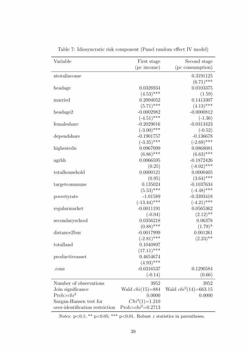
Table 7: Idiosyncratic risk component (Panel random effect IV model)

Variable First stage Second stage(pc income) (pc consumption)

ntotalincome 0.3191125(6.71)***

headage 0.0326934 0.0103375(4.53)*** (1.59)

married 0.2094052 0.1413307(5.71)*** (4.13)***

headage2 -0.0002982 -0.0000812(-4.51)*** (-1.36)

femaleshare -0.2029016 -0.0313423(-3.00)*** (-0.52)

dependshare -0.1901757 -0.136678(-3.35)*** (-2.69)***

highestedu 0.0967099 0.0868081(6.86)*** (6.63)***

agrhh 0.0066595 -0.1872426(0.25) (-8.02)***

totalhousehold 0.0000121 0.0000405(0.95) (3.64)***

targetcommune 0.135024 -0.1037634(5.53)*** (-4.48)***

povertyrate -1.01589 -0.3393418(-13.44)*** (-4.21)***

regularmarket -0.0011191 0.0565362(-0.04) (2.12)**

secondaryschool 0.0356218 0.06378(0.88)*** (1.79)*

distance2bus -0.0017999 0.001261(-2.81)*** (2.23)**

totalland 0.1040897(17.11)***

productiveasset 0.4654674(4.93)***

cons -0.0316537 0.1290584(-0.14) (0.66)

Number of observations 3952 3952Join significance Wald chi(15)=884 Wald chi2(14)=663.15Prob>chi2 0.0000 0.0000Sargan-Hansen test for Chi2(1)=1.210over-identification restriction Prob>chi2=0.2713

Notes: p<0.1; ** p<0.05; *** p<0.01. Robust z statistics in parentheses.

39

Table 8: Decomposition of average vulnerability during 2010-2012

VEU Poverty Covariate risk Idiosyncratic risk Unexplained risk

0.7108 0.4314 -0.3410 0.4288 0.1905

Source: Author’s calculation from VARHS 2010 and 2012.

components of Equation 12. A household’s VEU is the sum of four separate components.

The aggregate VEU and its components are presented in Table 8. The estimate of the

average VEU (0.7108) is our estimate of the vulnerability of the whole households. This

implies that the utility of the average household is 71 per cent less than the hypothetical

situation without any risk or inequality in consumption. This level of utility vulnerability

is lower than the estimation of Gaiha & Imai (2008) which is 0.7476 but much higher

than the estimation of Jha et al. (2013) which is around 0.3016. Idiosyncratic shocks

contribute considerably to the utility loss (approximately 60 per cent). However, the

negative sign of the aggregate risk component indicates that economic growth cancels

the negative covariate shocks and even reduce the vulnerability. We may argue that the

utility loss would be more serious if there had been less economic growth in rural Vietnam

during the period of 2010-2012.

Impact of health insurance on VEU and VEP

To estimate the impact of health insurance on vulnerability, we first calculate the propen-

sity scores for households covered in the data set. The probit regression is employed to

estimate the propensity score by default20. The dependent variable is health insurance

coverage which is represented by a dummy taking the value of one for the treatment group

and zero for the control group. There are two requirements for the explanatory variables

in order to get an accurate estimation of the propensity scores. First, the independent

variables need to be exogenous to the health insurance variable used as the dependent

variable (Heckman & Vytlacil 1999, Ravallion 2001). Therefore, we decide to choose ex-

20The Stata command pscore is employed in this study and the probit is used to estimate propensityscore by default. The balancing test is also provided. The estimated results are similar with the Statacommand ‘psmatch2 ’ (Table A2).

40

planatory variables from the 2010 VARHS rather than from the 2012 VARHS. Second,

the independent variables should affect both the vulnerability index and health insurance

coverage (Ravallion 2001). In this study, these variables include health insurance status

in 2010, health status, risk aversion, income, asset, age of household head, marital status

of the head, female share of the household, dependent share of the household, occupa-

tion and distance to the nearest bus station. Other commune variables representing the

covariate shocks that might affect health insurance decision such as drought, flood, epi-

demic, livestock disease and other shocks are also added to the regression. They are all

for the year 201021.

One might have a concern that compulsory and voluntary health insurance schemes

are treated equivalently in our analysis. However, during the time span of the data, the

difference between the two schemes would be trivial because of certain reasons: First, the

compulsory health insurance scheme in Vietnam is not strictly compulsory and therefore,

the coverage rate of this scheme is not 100 per cent for all groups of households (Table 5).

Households who are not fully subsidized in compulsory groups will go through a decision

making process similar to what households in voluntary groups will do. In addition, the

premium is quite small in comparison with other types of consumption; then although

households in compulsory groups are partly subsidized, the amount of money they have to

pay for a health insurance card is not much different from that of households in voluntary

scheme. Also, health insurance for the poor and health insurance for children under six

years of age, who are compulsorily insured and fully subsidized, are excluded to keep the

incentive gap at the minimal level. For households with labor contract, they are supposed

to receive health insurance card from their employers. But if employers refuse to provide

health insurance illegally and intentionally, employees can choose to stay or find a better

job with health insurance (Monheit & Vistnes 2008). Hence, their probability of having a

health insurance card might depend on their risk preference or factors representing their

negotiating power such as education, age rather than types of health insurance schemes.

21The balancing property is satisfied for 7 blocks with the pscore Stata command.

41

Table 9 shows the results of the probit regression on health insurance. As can be

seen from the table, the insured and the uninsured household are statistically different in

several characteristics. For instance, households who have health insurance in 2010 are

more likely to have health insurance in 2012. Households with a higher income tend to

own at least one health insurance in 2012. Households with higher proportion of females

increase the probability of purchasing health insurance. Similarly, households living in

an area with a high incidence of epidemics tend to have health insurance. However,

living in a commune with a high incidence of drought and livestock disease reduce the

probability of purchasing health insurance. This might be because these types of risks

do not affect household member’s health status. Also, households with agricultural jobs

or with a higher dependent share have less demand on health insurance. In our study,

health status defined by the number of days on sick leave during past 12 month (in survey

2010) does not affect health insurance status in 2012.

In our paper, it seems that risk aversion indexes (both the cumulative risk aversion and

the absolute risk aversion) do not affect the decision to purchase health insurance because

the estimated coefficients are negative and insignificant (Table 9)22. This result contrasts

with Condliffe & Fiorentino (2014) where individuals who are more likely to engage risk

behavior are less likely to carry health insurance. There are four possible reasons for this.

First, risk aversion effect in our paper is offset by ‘rigidity effect’ that individuals are

least likely to change their current insurance plan. Several previous studies have pointed

out that individuals tend to appreciate the value of their current health insurance plan;

therefore, they are less likely to purchase health insurance if they have never bought

it before (Costa-Font & Garcia-Villar 2009, Friedman 1974, Marquis & Holmer 1996)23.

In our result, the impact of health insurance status in 2010 was positive and strongly

significant. Therefore, we have reason to believe that the ‘rigidity effect’ exists. Second,

22In Table A3 in the Appendix, we classified households into three different groups of risk attitudeand found that households with low risk aversion (i.e. prefer taking risk) are more likely to have healthinsurance.

23Thaler (1980) calls this the “endowment effect”; Samuelson & Zeckhauser (1988) call this a “statusquo” bias; and Costa-Font & Garcia-Villar (2009) call this the “captive preference”.

42

households might prefer other types of insurance over health insurance because the gain

from health insurance is uncertain and ambiguous (Marquis & Holmer 1996)24. Third, the

effect of individual risk aversion might be stronger for decisions taken in the near future

and then might reduce considerably in next two years (which is the duration between the

two surveys). Once we try to estimate the impact of risk aversion on any type of insurance

coverage, we find the positive and significant effects in the same year but not significant in

the next two years (Table A4 and Table A5 in Appendix)25. Similarly, Bernstein (2009)

shows that risk preference does not explain the disparity in health insurance coverage

and any increase in insurance coverage is closely associated with changes that result in

insurance being more affordable and accessible such as in socio-economic circumstances,

incomes, marital status and education. Four, this might reflect the fact that the market

for health insurance is limited and mainly provided by few state companies. A health

insurance purchasing decision is restrained not only by limited health insurance choices,

but also by the complicated purchasing process. For instance, households are strictly

required to enroll all household members who have a name on the household certificate,

despite the fact that some members had migrated to other places. The complexity for

enrolment criteria and process hinders the increase of the coverage as pointed out in

Matsushima & Yamada (2014).

Table 10 reports the health insurance impact on vulnerability using propensity score

matching and the difference-in-difference method. The kernel-matching estimator is ap-

plied with a bandwidth of 0.06 for interpretation26. The first and second columns present

the difference between treatment and control groups in 2012 and 2010, respectively. They

are estimated components of ATT2012,X,H2010 . Therefore, the difference-in-difference esti-

mates in the last column are attributed to the health insurance impact, or ATT2012,X,H2010 .

24Vietnamese newspapers note that in Phuong (2013) and Trang (2012).25However, we cannot deny that simultaneous bias with this specification because independent variable

and dependent variables in the probit model are collected in the same survey.26Bootstrapping for the nearest neighbour matching may not provide accurate standard errors (Abadie

& Imbens 2008) even though the nearest neighbour matching and the kernel matching yield similarresults.

43

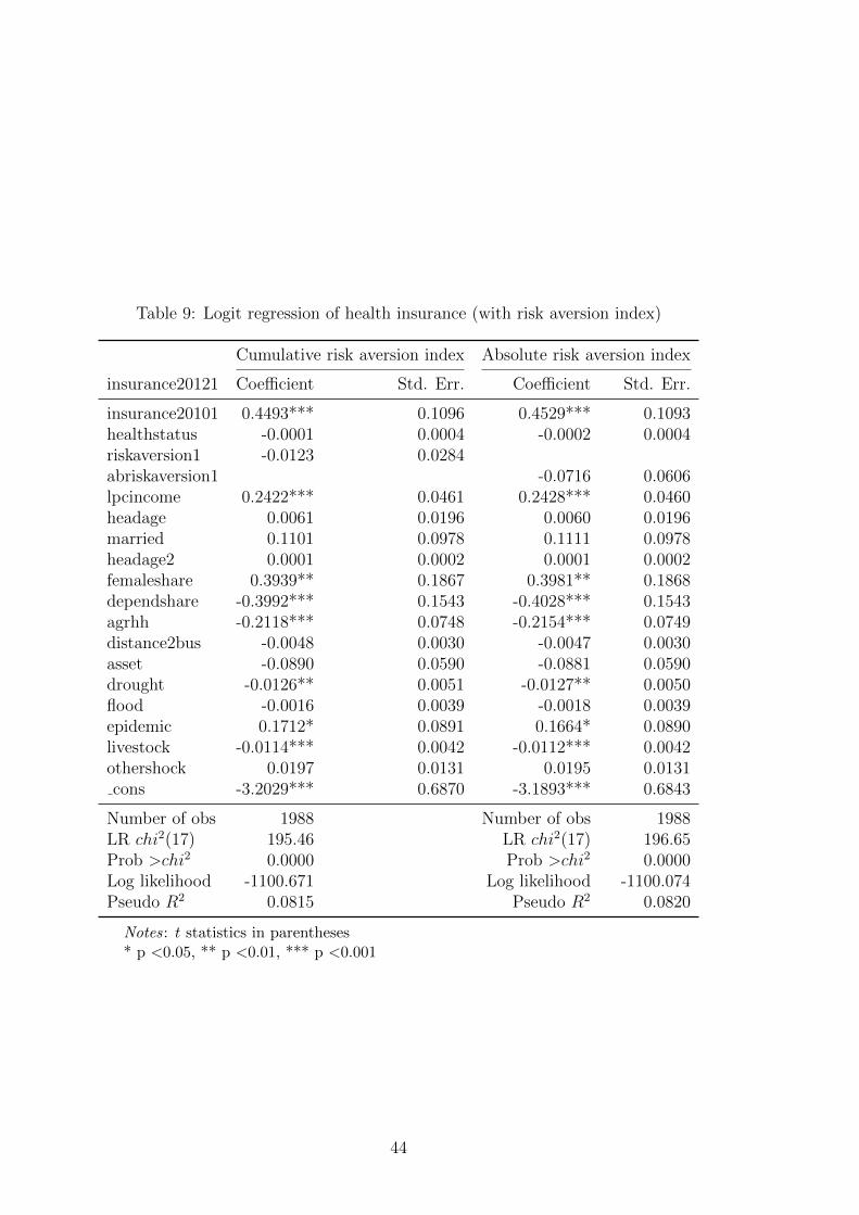
Table 9: Logit regression of health insurance (with risk aversion index)

Cumulative risk aversion index Absolute risk aversion index

insurance20121 Coefficient Std. Err. Coefficient Std. Err.

insurance20101 0.4493*** 0.1096 0.4529*** 0.1093healthstatus -0.0001 0.0004 -0.0002 0.0004riskaversion1 -0.0123 0.0284abriskaversion1 -0.0716 0.0606lpcincome 0.2422*** 0.0461 0.2428*** 0.0460headage 0.0061 0.0196 0.0060 0.0196married 0.1101 0.0978 0.1111 0.0978headage2 0.0001 0.0002 0.0001 0.0002femaleshare 0.3939** 0.1867 0.3981** 0.1868dependshare -0.3992*** 0.1543 -0.4028*** 0.1543agrhh -0.2118*** 0.0748 -0.2154*** 0.0749distance2bus -0.0048 0.0030 -0.0047 0.0030asset -0.0890 0.0590 -0.0881 0.0590drought -0.0126** 0.0051 -0.0127** 0.0050flood -0.0016 0.0039 -0.0018 0.0039epidemic 0.1712* 0.0891 0.1664* 0.0890livestock -0.0114*** 0.0042 -0.0112*** 0.0042othershock 0.0197 0.0131 0.0195 0.0131cons -3.2029*** 0.6870 -3.1893*** 0.6843

Number of obs 1988 Number of obs 1988LR chi2(17) 195.46 LR chi2(17) 196.65Prob >chi2 0.0000 Prob >chi2 0.0000Log likelihood -1100.671 Log likelihood -1100.074Pseudo R2 0.0815 Pseudo R2 0.0820

Notes: t statistics in parentheses* p <0.05, ** p <0.01, *** p <0.001

44

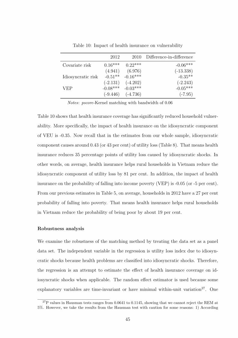
Table 10: Impact of health insurance on vulnerability

2012 2010 Difference-in-difference

Covariate risk 0.16*** 0.22*** -0.06***(4.941) (6.976) (-13.338)

Idiosyncratic risk -0.51** -0.16*** -0.35**(-2.131) (-4.202) (-2.243)

VEP -0.08*** -0.03*** -0.05***(-9.446) (-4.736) (-7.95)

Notes: pscore-Kernel matching with bandwidth of 0.06

Table 10 shows that health insurance coverage has significantly reduced household vulner-

ability. More specifically, the impact of health insurance on the idiosyncratic component

of VEU is -0.35. Now recall that in the estimates from our whole sample, idiosyncratic

component causes around 0.43 (or 43 per cent) of utility loss (Table 8). That means health

insurance reduces 35 percentage points of utility loss caused by idiosyncratic shocks. In

other words, on average, health insurance helps rural households in Vietnam reduce the

idiosyncratic component of utility loss by 81 per cent. In addition, the impact of health

insurance on the probability of falling into income poverty (VEP) is -0.05 (or -5 per cent).

From our previous estimates in Table 5, on average, households in 2012 have a 27 per cent

probability of falling into poverty. That means health insurance helps rural households

in Vietnam reduce the probability of being poor by about 19 per cent.

Robustness analysis

We examine the robustness of the matching method by treating the data set as a panel

data set. The independent variable in the regression is utility loss index due to idiosyn-

cratic shocks because health problems are classified into idiosyncratic shocks. Therefore,

the regression is an attempt to estimate the effect of health insurance coverage on id-

iosyncratic shocks when applicable. The random effect estimator is used because some

explanatory variables are time-invariant or have minimal within-unit variation27. One

27P values in Hausman tests ranges from 0.0641 to 0.1145, showing that we cannot reject the REM at5%. However, we take the results from the Hausman test with caution for some reasons: 1) According

45

example is our key explanatory variable representing health insurance coverage. Risk

aversion index is used as an explanatory variable in addition to other household charac-

teristics and commune characteristics so that we can minimize the possible correlation

between error term and explanatory variables.

Table 11 reports the results for the models used to estimate the impact of health

insurance coverage on household vulnerability. Absolute risk aversion index is used as an

explanatory variable in this case28. Without control variables, the estimated coefficient of

health insurance is -0.26 and significant. This implies health insurance coverage helps to

reduce utility loss by 26 percentage points. Using the between estimator for panel data,

we have larger impact of health insurance at -0.56. If we add household characteristics

and commune characteristics into the regression, the random effect estimator produces

an impact of health insurance of about -0.23 and the between estimator gives an impact

of around -0.49.

Because of the data collection timing, we do not know when households bought health

insurance. It could have been at the beginning or at the end of the year. Therefore, we

assume that the impact of health insurance coverage should be the impact of total health

insurance during the time between the two surveys. Therefore, in our regression, the ex-

planatory variable becomes the total health insurance that a household has during 2010

and 2012. The number is the sum of health insurance they have in the 2010 survey and in

the 2012 survey. Dependent variables are the same. As seen in Table 12, with the random

effect estimator, having a health insurance will reduce utility loss about -0.21. Similarly,

with the between estimator, the impact of health insurance is about -0.24. Although

these results are not exactly the same as the estimates from the matching method, they

to Jones et al. (2013), in a finite sample, a standard application of the Hausman test may not lead toa reliable test statistic. 2) According to Clark & Linzer (2014), when the independent variable exhibitsonly minimal within-unit variation, the random-effects model will tend to produce superior estimates ofβ when there are few units or observations per unit, and when the correlation between the independentvariable and unit effects is relatively low. An increase in efficiency can offset an increase in bias even theHausman test supports the use of fixed effect regression.

28Results with cumulative risk aversion index are also provided in the Table A10 and A11 of Appendix.Hausman tests favour REM because p-values vary from 0.0771 to 0.1321.

46

Table 11: Impact of health insurance coverage on idiosyncratic VEU(health insurance at the time of interview, absolute)

Random Between Random Betweeneffect variation effect variation

Health insurance -0.261*** -0.558*** -0.231*** -0.486**(Yes/No at the time (0.043) (0.160) (0.069) (0.167)of interview)Absolute risk aversion -0.164* -0.082 -0.129* -0.104

(0.088) (0.165) (0.076) (0.163)Health status -0.030 -0.009 -0.068 -0.067

(0.032) (0.065) (0.059) (0.066)Per capita income (log) -0.270*** -0.251*** -0.174*** -0.163**

(0.058) (0.060) (0.045) (0.066)Household characteristics No No Yes YesCommune characteristics No No Yes Yes

N 3952 3952 3952 3952R2 0.019 0.066F 9.524 5.991p 0.000 0.000 0.000 0.000

Notes: Standard errors in parentheses* p <0.05, ** p <0.01, *** p <0.001

47

Table 12: Impact of health insurance coverage on idiosyncratic VEU(total health insurances across surveys, absolute)

Random Between Random Betweeneffect variation effect variation

Health insurance -0.274*** -0.269*** -0.214*** -0.235**(Total insurance across surveys) (0.044) (0.080) (0.057) (0.084)Absolute risk aversion -0.164* -0.082 -0.133* -0.105

(0.088) (0.165) (0.077) (0.163)Health status -0.029 -0.008 -0.070 -0.066

(0.032) (0.065) (0.059) (0.066)Per capita income (log) -0.239*** -0.251*** -0.161*** -0.163**

(0.055) (0.060) (0.043) (0.067)Household characteristics No No Yes YesCommune characteristics No No Yes Yes

N 3952 3952 3952 3952R2 0.018 0.065F 9.273 5.961p 0.000 0.000 0.000 0.000

Notes: Standard errors in parentheses* p <0.05, ** p <0.01, *** p <0.001

reinforce our findings about the negative and significant impact of health insurance cover-

age on household vulnerability. Although we have captured various factors in our model

specification and the difference-in-difference method helps to eliminate the impact of un-

observed time-invariant factors, there is still a concern about other unobserved variables

that might affect both health insurance enrolment and vulnerability. If this situation ex-

ists, our matching estimators violate the conditional independence or unconfoundedness

assumption (CIA) and may lead to a hidden bias. In this paper, we adopt a sensitivity

analysis proposed by Ichino et al. (2008), building on Rosenbaum & Rubin (1983) and

Rosenbaum (1987). They suggest that if the CIA is not satisfied given observables but

it is satisfied if one could observe an additional binary variable (confounder), then this

potential confounder could be simulated in the data and used as an additional covariate

in combination with the preferred matching estimator. The comparison of the estimates

obtained with and without matching on the simulated confounder shows to what extent

the baseline results are robust to specific sources of failure of the CIA, since the distribu-

48

Table 13: Simulation-based sensitivity analysis for matching estimators (2010,confounders: young and low education)

ATT2010 Standard error Outcome effect Selection effect

Young -0.147 0.008 1.623 0.456Low education -0.154 0.004 3.552 0.582

Notes: Based on the sensitivity analysis with kernel matching algorithm withbetween-imputation standard error. The binary transformation of the outcome isalong the 75 centile. Young variable (=1 if age is less than 41 years, or the 25centile) and low education (=1 if households do not have any certificate). Boththe outcome and the selection effect are odds ratios from logit estimations.

tion of the simulated variable can be constructed to capture different hypotheses on the

nature of potential confounding factors (Nannicini 2007).

In this study, we use two covariates to simulate the confounder namely: young (age of

household head is less than 47, or in the 25th centile of age distribution) and low education

(with no diploma). These covariates are selected to capture the effect of unobservable

factors like ability and experience. If the ATT estimates change dramatically with respect

to these confounders, our results might be not robust. We employ the kernel matching

algorithm with between-imputation standard errors. Since our outcome variable is con-

tinuous, the confounders is stimulated on the basis of the binary transformation of the

outcome along the 75th centile. The results of the sensitivity analysis are presented in

Table 13 and Table 14. For both confounders, the simulated ATT estimated are very close

to the baseline estimates. The outcome and selection effect on vulnerability is positive

but not very large. The results confirm a robustness of the matching estimates.

7 Policy implication and conclusion

Health shocks are one of the major cause of vulnerability and poverty in Vietnam. There-

fore, the government of Vietnam has endeavored to increase the health insurance enroll-

ment in order to attain its goal of universal health insurance coverage. This paper is an

attempt to provide empirical evidence for an effective health policy in Vietnam. To the

49

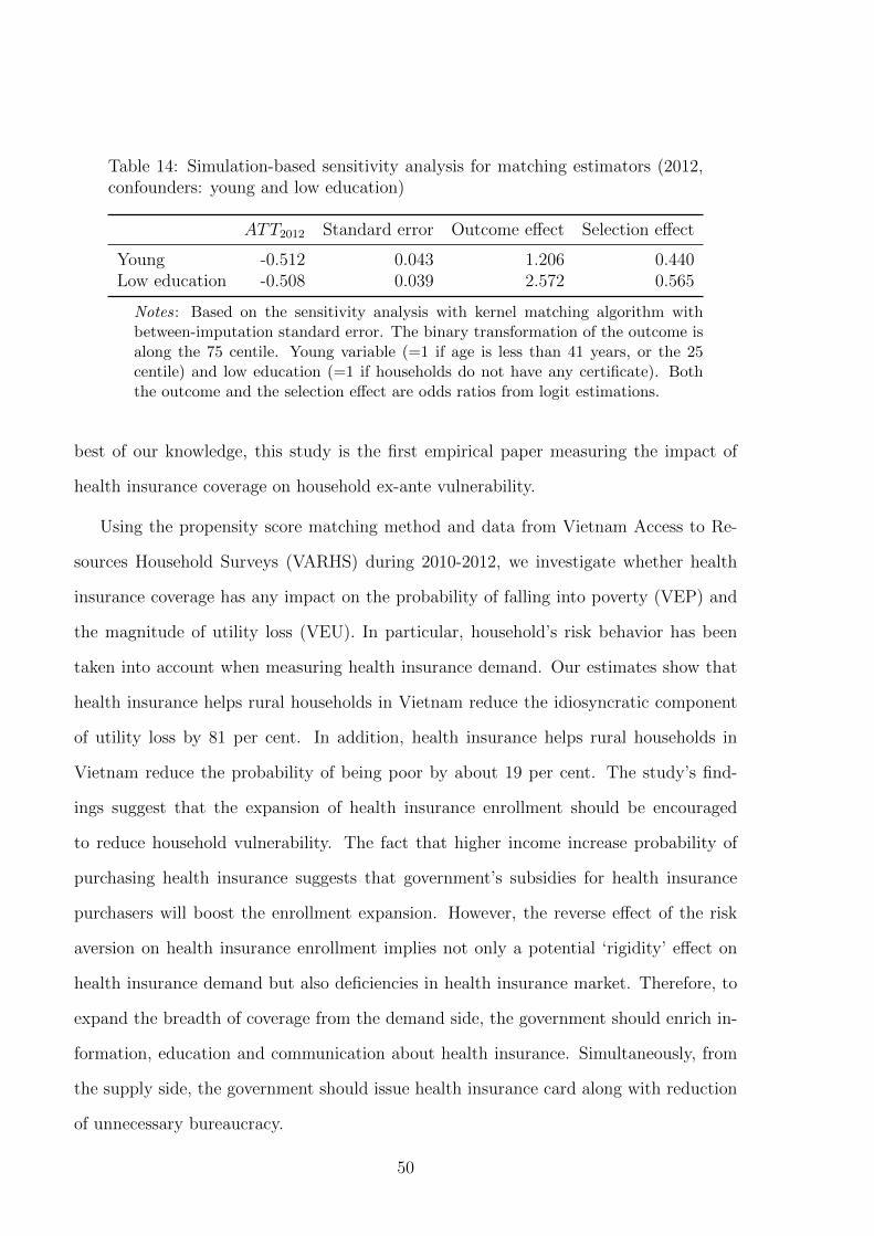
Table 14: Simulation-based sensitivity analysis for matching estimators (2012,confounders: young and low education)

ATT2012 Standard error Outcome effect Selection effect

Young -0.512 0.043 1.206 0.440Low education -0.508 0.039 2.572 0.565

Notes: Based on the sensitivity analysis with kernel matching algorithm withbetween-imputation standard error. The binary transformation of the outcome isalong the 75 centile. Young variable (=1 if age is less than 41 years, or the 25centile) and low education (=1 if households do not have any certificate). Boththe outcome and the selection effect are odds ratios from logit estimations.

best of our knowledge, this study is the first empirical paper measuring the impact of

health insurance coverage on household ex-ante vulnerability.

Using the propensity score matching method and data from Vietnam Access to Re-

sources Household Surveys (VARHS) during 2010-2012, we investigate whether health

insurance coverage has any impact on the probability of falling into poverty (VEP) and

the magnitude of utility loss (VEU). In particular, household’s risk behavior has been

taken into account when measuring health insurance demand. Our estimates show that

health insurance helps rural households in Vietnam reduce the idiosyncratic component

of utility loss by 81 per cent. In addition, health insurance helps rural households in

Vietnam reduce the probability of being poor by about 19 per cent. The study’s find-

ings suggest that the expansion of health insurance enrollment should be encouraged

to reduce household vulnerability. The fact that higher income increase probability of

purchasing health insurance suggests that government’s subsidies for health insurance

purchasers will boost the enrollment expansion. However, the reverse effect of the risk

aversion on health insurance enrollment implies not only a potential ‘rigidity’ effect on

health insurance demand but also deficiencies in health insurance market. Therefore, to

expand the breadth of coverage from the demand side, the government should enrich in-

formation, education and communication about health insurance. Simultaneously, from

the supply side, the government should issue health insurance card along with reduction

of unnecessary bureaucracy.

50

Finally yet importantly, although we have reasons to believe the estimation bias in

this paper is minimal, future studies could improve upon our results if the data improves

in certain regards. First, the two identification assumptions in the PSM method can

be checked. In addition, questionnaires about the household health insurance coverage

can help to differentiate between compulsory and voluntary schemes; and questionnaires

about risk attitudes should be designed to increase the payoff and therefore, draw atten-

tion to the answers.

References

Abadie, A. & Imbens, G. W. (2008), ‘On the failure of the bootstrap for matching esti-

mators’, Econometrica 76(6), 1537–1557.

Abdellaoui, M. (2000), ‘Parameter-free elicitation of utility and probability weighting

functions’, Management Science 46(11), 1497–1512.

Abegunde, D. & Stanciole, A. (2008), ‘The economic impact of chronic diseases: how do

households respond to shocks? evidence from russia’, Social science & medicine (1982)

66(11), 2296.

Adkins, L. C. & Hill, C. (2011), Using Stata for principles of econometrics, Wiley Global

Education.

Amemiya, T. (1977), ‘The maximum likelihood and the nonlinear three-stage least

squares estimator in the general nonlinear simultaneous equation model’, Econometrica

45(4), 955–968.

URL: http://www.jstor.org/stable/1912684

Andersen, S., Harrison, G. W., Lau, M. I. & Rutstrm, E. E. (2008), ‘Eliciting risk and

time preferences’, Econometrica 76(3), 583–618.

Arrow, K. J. (1965), Aspects of the theory of risk-bearing, Yrj Jahnssonin Sti.

51

Bales, S., Knowles, J., Axelson, H., Minh, P., Luong, D. & Oanh, T. (2007), ‘The early

impact of decision 139 in vietnam: an application of propensity score matching’, Report

to the Ministry of Health of Vietnam .

Barseghyan, L., Molinari, F., O’Donoghue, T. & Teitelbaum, J. C. (2013), ‘The na-

ture of risk preferences: Evidence from insurance choices’, American Economic Review

103(6), 2499–2529.

Benartzi, S. & Thaler, R. H. (1995), ‘Myopic loss aversion and the equity premium puzzle’,

The Quarterly Journal of Economics pp. 73–92.

Bernoulli, D. (1954), ‘Exposition of a new theory on the measurement of risk’, Econo-

metrica: Journal of the Econometric Society pp. 23–36.

Bernstein, D. P. (2009), ‘Economic factors, attitudes towards risk, and health insurance

coverage for young adults’, Attitudes Towards Risk, and Health Insurance Coverage for

Young Adults (May 14, 2009) .

Bleichrodt, H. & Gafni, A. (1996), ‘Time preference, the discounted utility model and

health’, Journal of Health Economics 15(1), 49–66.

URL: http://www.sciencedirect.com/science/article/pii/0167629695000313

Bleichrodt, H. & Pinto, J. L. (2000), ‘A parameter-free elicitation of the probability

weighting function in medical decision analysis’, Management science 46(11), 1485–

1496.

Bleichrodt, H. & Pinto, J. L. (2002), ‘Loss aversion and scale compatibility in two-

attribute trade-offs’, Journal of Mathematical Psychology 46(3), 315–337.

Booij, A. S. & Van de Kuilen, G. (2009), ‘A parameter-free analysis of the utility of money

for the general population under prospect theory’, Journal of Economic Psychology

30(4), 651–666.

52

Bowman, D., Minehart, D. & Rabin, M. (1999), ‘Loss aversion in a consumption–savings

model’, Journal of Economic Behavior & Organization 38(2), 155–178.

Bridges, J. (2003), ‘Stated preference methods in health care evaluation: an emerging

methodological paradigm in health economics’, Applied health economics and health

policy 2(4), 213–224.

Calvo, C. & Dercon, S. (2005), Measuring individual vulnerability, Technical report,

University of Oxford.

Camerer, C., Babcock, L., Loewenstein, G. & Thaler, R. (1997), ‘Labor supply of new

york city cabdrivers: One day at a time’, The Quarterly Journal of Economics pp. 407–

441.

Carter, M. R., Little, P. D., Mogues, T. & Negatu, W. (2007), ‘Poverty traps and natural

disasters in ethiopia and honduras’, World Development 35(5), 835–856.

URL: http://www.sciencedirect.com/science/article/pii/S0305750X07000149

Chaudhuri, A. & Roy, K. (2008), ‘Changes in out-of-pocket payments for healthcare in

vietnam and its impact on equity in payments, 1992-2002’, Health Policy 88(1), 38–48.

Chaudhuri, S. (2003), ‘Assessing vulnerability to poverty: concepts, empirical methods

and illustrative examples’, Department of Economics, Columbia University, New York

.

Chaudhuri, S., Jalan, J. & Suryahadi, A. (2002), ‘Assessing household vulnerability to

poverty from cross-sectional data: A methodology and estimates from indonesia’.

Clark, T. S. & Linzer, D. A. (2014), ‘Should i use fixed or random effects?’, Political

Science Research and Methods pp. 1–10.

Condliffe, S. & Fiorentino, G. T. (2014), ‘The impact of risk preference on health in-

surance and health expenditures in the united states’, Applied Economics Letters

21(9), 613–616.

53

Costa-Font, J. & Garcia-Villar, J. (2009), ‘Risk attitudes and the demand for private

health insurance: the importance of captive preferences’, Annals of Public and Coop-

erative Economics 80(4), 499–519.

Cunningham, W. & Maloney, W. F. (2000), ‘Measuring vulnerability: who suffered in

the 1995 mexican crisis?’, World Bank mimeo .

Dercon, S. (2004), ‘Growth and shocks: Evidence from rural ethiopia’, Journal of Devel-

opment Economics 74(2), 309–329.

Dercon, S. (2005), Risk, insurance, and poverty: A review, Insurance against Poverty,

Oxford, Oxford University Press.

Duflo, A. (2005), ‘Health shocks and economic vulnerability in rural india: break the

vicious circle’, Centre for Micro Finance Research Working Paper, Center for Micro

Finance, IFMR .

Einav, L., Finkelstein, A., Pascu, I. & Cullen, M. (2010), How general are risk preference?

choices under uncertainty in different domains, Technical report, National Bureau of

Economic Research.

Fafchamps, M. & Lund, S. (2003), ‘Risk-sharing networks in rural philippines’, Journal

of development Economics 71(2), 261–287.

Fafchamps, M., Udry, C. & Czukas, K. (1998), ‘Drought and saving in west africa: are

livestock a buffer stock?’, Journal of Development Economics 55(2), 273–305.

URL: http://www.sciencedirect.com/science/article/pii/S0304387898000376

Fehr, E., Goette, L. & Zehnder, C. (2007), ‘The behavioral economics of the labor market:

Central findings and their policy implications’, Unpublished manuscript, Boston Federal

Reserve .

Friedman, B. (1974), ‘Risk aversion and the consumer choice of health insurance option’,

The Review of Economics and Statistics pp. 209–214.

54

Friedman, M. & Savage, L. J. (1948), ‘The utility analysis of choices involving risk’, The

journal of political economy pp. 279–304.

Gachter, S., Johnson, E. J. & Herrmann, A. (2010), Individual-level loss aversion in

riskless and risky choices, Technical report, CeDEx discussion paper series.

Gaiha, R. & Imai, K. S. (2008), Measuring vulnerability and poverty: Estimates for rural

india, Technical report, World Institute for Development Economic Research (UNU-

WIDER).

Gertler, P. & Gruber, J. (2002), ‘Insuring consumption against illness’, The American

Economic Review 92(1), 51–70.

URL: http://www.jstor.org/stable/3083321

Gertler, P., Levine, D. I. & Moretti, E. (2009), ‘Do microfinance programs help families

insure consumption against illness?’, Health Economics 18(3), 257–273.

URL: http://dx.doi.org/10.1002/hec.1372

Glewwe, P. & Hall, G. (1998), ‘Are some groups more vulnerable to macroeconomic shocks

than others? hypothesis tests based on panel data from peru’, Journal of Development

Economics 56(1), 181–206.

Goette, L., Huffman, D. & Fehr, E. (2004), ‘Loss aversion and labor supply’, Journal of

the European Economic Association 2(2-3), 216–228.

Gujarati, D. N. (2011), Econometrics by example, Palgrave Macmillan Hampshire, UK.

Haigh, M. S. & List, J. A. (2005), ‘Do professional traders exhibit myopic loss aversion?

an experimental analysis’, The Journal of Finance 60(1), 523–534.

Harrower, S. & Hoddinott, J. (2004), Consumption smoothing and vulnerability in the

Zone Lacustre, Mali, International Food Policy Research Institute.

55

Hartog, J., Ferrer-i Carbonell, A. & Jonker, N. (2002), ‘Linking measured risk aversion

to individual characteristics’, Kyklos 55(1), 3–26.

Hasegawa, M. (2010), Risk coping measures against different types of shocks: Empiri-

cal evidence from vietnam household living standard survey, Technical report, Osaka

School of International Public Policy, Osaka University.

Heckman, J. J. & Vytlacil, E. J. (1999), ‘Local instrumental variables and latent variable

models for identifying and bounding treatment effects’, Proceedings of the national

Academy of Sciences 96(8), 4730–4734.

Heidhues, P. & Koszegi, B. (2008), ‘Competition and price variation when consumers are

loss averse’, The American Economic Review pp. 1245–1268.

Hoddinott, J. & Quisumbing, A. (2003), ‘Methods for microeconometric risk and vulner-

ability assessments’.

Hort, K. (2011), Private hospitals in vietnam: Recent growth and role in the health

sector, Technical report, University of Melbourne.

Ichino, A., Mealli, F. & Nannicini, T. (2008), ‘From temporary help jobs to permanent

employment: What can we learn from matching estimators and their sensitivity?’,

Journal of Applied Econometrics 23(3), 305–327.

Imai, K. S., Gaiha, R. & Kang, W. (2011), ‘Vulnerability and poverty dynamics in viet-

nam’, Applied Economics 43(25), 3603–3618.

Isaac, R. M. & James, D. (2000), ‘Just who are you calling risk averse?’, Journal of Risk

and Uncertainty 20(2), 177–187.

JAHR (2009), Joint annual health review, Technical report, Ministry of Health of Viet-

nam, Health Partnership Group, Hanoi.

56

JAHR (2013), Joint annual health review, Technical report, Ministry of Health of Viet-

nam, Health Partnership Group, Hanoi.

Jalan, J. & Ravallion, M. (1999), ‘Are the poor less well insured? evidence on vulnerability

to income risk in rural china’, Journal of development economics 58(1), 61–81.

Jha, R., Dang, T. & Tashrifov, Y. (2010), ‘Economic vulnerability and poverty in tajik-

istan’, Economic Change and Restructuring 43(2), 95–112.

Jha, R., Kang, W., Nagarajan, H. K. & Pradhan, K. C. (2013), Vulnerability and re-

sponses to risks in rural india, Technical report, The Australian National University,

Australia South Asia Research Centre.

Jones, A. M., Rice, N., d’Uva, T. B. & Balia, S. (2013), Applied health economics, Rout-

ledge.

Jowett, M., Contoyannis, P. & Vinh, N. D. (2003), ‘The impact of public voluntary health

insurance on private health expenditures in vietnam’, Social Science &amp; Medicine

56(2), 333–342.

URL: http://www.sciencedirect.com/science/article/pii/S027795360200031X

Jowett, M., Deolalikar, A. & Martinsson, P. (2004), ‘Health insurance and treatment

seeking behaviour: evidence from a low?income country’, Health Economics 13(9), 845–

857.

Kahneman, D. & Tversky, A. (1979), ‘Prospect theory: An analysis of decision under

risk’, Econometrica 47(2), 263–291.

URL: http://www.jstor.org.virtual.anu.edu.au/stable/1914185

Kent, R. (2002), ‘Reduction of catastrophic health care expenditures by a community-

based health insurance scheme in gujarat, india: current experiences and challenges’,

Bulletin of the World Health Organization 80.

57

Khandker, S. R. (1998), Fighting poverty with microcredit: experience in Bangladesh,

Oxford University Press.

Kim, T., Oanh, T., Shuangge, M., Pham, D., Khuat, G. & Ruger, J. (2011), ‘Coping

with health care expenses among poor households: evidence from a rural commune in

vietnam’, Social Science & Medicine .

Klasen, S. & Waibel, H. (2010), Vulnerability to poverty: theory, measurement and de-

terminants, Palgrave Macmillan.

Kruk, M., Goldmann, E. & Galea, S. (2009), ‘Borrowing and selling to pay for health

care in low-and middle-income countries’, Health Affairs 28(4), 1056–1066.

Ligon, E. & Schechter, L. (2003), ‘Measuring vulnerability’, The Economic Journal

113(486), C95–C102.

Lusk, J. L. & Coble, K. H. (2005), ‘Risk perceptions, risk preference, and acceptance of

risky food’, American Journal of Agricultural Economics 87(2), 393–405.

Markussen, T., Tarp, F. & Tuan, N. D. A. (2012), ‘Inter-and intra-farm land fragmenta-

tion in vietnam’, Policy Brief 6.

Marquis, M. S. & Holmer, M. R. (1996), ‘Alternative models of choice under uncertainty

and demand for health insurance’, The Review of Economics and Statistics pp. 421–427.

Matsushima, M. & Yamada, H. (2014), ‘Public health insurance in vietnam towards

universal coverage: Identifying the challenges, issues, and problems in its design and

organisational practices’, ?? 29(4), 289–297.

McIntyre, D., Thiede, M., Dahlgren, G. & Whitehead, M. (2006), ‘What are the economic

consequences for households of illness and of paying for health care in low- and middle-

income country contexts?’, Social Science & Medicine 62(4), 858–865.

URL: http://www.sciencedirect.com/science/article/pii/S0277953605003631

58

Monheit, A. C. & Vistnes, J. P. (2008), ‘Health insurance enrollment decisions: prefer-

ences for coverage, worker sorting, and insurance take-up’, INQUIRY: The Journal of

Health Care Organization, Provision, and Financing 45(2), 153–167.

Montalbano, P. & Magrini, E. (2012), ‘Trade openness and vulnerability to poverty:

Vietnam in the long-run (1992-2008)’.

Morduch, J. (1994), ‘Poverty and vulnerability’, The American Economic Review

84(2), 221–225.

Morduch, J. (1999), ‘The microfinance promise’, Journal of economic literature pp. 1569–

1614.

Morduch, J. (2004), ‘Consumption smoothing across space’, Dercon, Insurance against

Poverty. Oxford University Press, New York and Oxford .

Nannicini, T. (2007), ‘Simulation-based sensitivity analysis for matching estimators’,

Stata Journal 7(3), 334.

Nguyen, C. (2010), Public health services and health care utilization in viet nam, Tech-

nical report, University Library of Munich, Germany.

Nguyen, C. V. (2012), ‘The impact of voluntary health insurance on health care utilization

and out-of-pocket payments: New evidence for vietnam’, Health Economics 21(8), 946–

966.

Nightingale, S. (1988), ‘Risk preference and admitting rates of emergency room physi-

cians’, Medical care pp. 84–87.

Nightingale, S. & Grant, M. (1988), ‘Risk preference and decision making in critical care

situations’, Chest 93(4), 684–687.

URL: http://dx.doi.org/10.1378/chest.93.4.684

59

Odean, T. (1998), ‘Are investors reluctant to realize their losses?’, The Journal of finance

53(5), 1775–1798.

Phelps, C. E. (2013), Health economics, 5th edn, Pearson Higher Education.

Phuong, N. (2013), ‘Households do not acknowledge the benefit of health insurance’.

URL: http://vnexpress.net/tin-tuc/thoi-su/nguoi-dan-chua-thay-loi-khi-mua-bao-

hiem-y-te-2907430.html

Picone, G., Sloan, F. & Taylor Jr, D. (2004), ‘Effects of risk and time preference and

expected longevity on demand for medical tests’, Journal of Risk and Uncertainty

28(1), 39–53.

Pratt, J. W. (1964), ‘Risk aversion in the small and in the large’, Econometrica: Journal

of the Econometric Society pp. 122–136.

Puhazhendi, V. & Badatya, K. (2002), ‘Self help group-bank linkage programme for rural

poor in india: An impact assessment’, New Delhi, India .

Ravallion, M. (2001), ‘Growth, inequality and poverty: looking beyond averages’, World

development 29(11), 1803–1815.

Richardson, J. (1994), ‘Cost utility analysis: what should be measured?’, Social science

& medicine 39(1), 7–21.

Rosenbaum, P. R. (1987), ‘Sensitivity analysis for certain permutation inferences in

matched observational studies’, Biometrika 74(1), 13–26.

Rosenbaum, P. R. & Rubin, D. B. (1983), ‘Assessing sensitivity to an unobserved bi-

nary covariate in an observational study with binary outcome’, Journal of the Royal

Statistical Society. Series B (Methodological) pp. 212–218.

Rosenzweig, M. R. & Wolpin, K. I. (1993), ‘Credit market constraints, consumption

60

smoothing, and the accumulation of durable production assets in low-income countries:

Investments in bullocks in india’, Journal of political economy pp. 223–244.

Rothschild, M. & Stiglitz, J. E. (1970), ‘Increasing risk: I. a definition’, Journal of

Economic theory 2(3), 225–243.

Rousseau, T. (2014), ‘Social health insurance’.

Samuelson, W. & Zeckhauser, R. (1988), ‘Status quo bias in decision making’, Journal

of risk and uncertainty 1(1), 7–59.

Sauerborn, R., Adams, A. & Hien, M. (1996), ‘Household strategies to cope with the

economic costs of illness’, Social Science & Medicine 43(3), 291–301.

URL: http://www.sciencedirect.com/science/article/pii/0277953695003754

Sepehri, A., Sarma, S. & Oguzoglu, U. (2011), ‘Does the financial protection of health

insurance vary across providers? vietnams experience’, Social Science &amp; Medicine

73(4), 559–567.

URL: http://www.sciencedirect.com/science/article/pii/S0277953611003546

Sepehri, A., Sarma, S. & Simpson, W. (2006), ‘Does non-profit health insurance reduce

financial burden? evidence from the vietnam living standards survey panel’, Health

economics 15(6), 603–616.

Skoufias, E. & Quisumbing, A. R. (2005), ‘Consumption insurance and vulnerability to

poverty: A synthesis of the evidence from bangladesh, ethiopia, mali, mexico and

russia’, The European journal of development research 17(1), 24–58.

Somanathan, Aparnaa; Tandon, A. D. H. L. H. K. L. F.-P. H. L. (2014), Moving toward

universal coverage of social health insurance in vietnam : assessment and options,

Technical Report 89066, World Bank Group, Washington, DC.

URL: http://documents.worldbank.org/curated/en/2014/06/19776955/moving-

toward-universal-coverage-social-health-insurance-vietnam-assessment-options

61

Starmer, C. (2000), ‘Developments in non-expected utility theory: The hunt for a de-

scriptive theory of choice under risk’, Journal of economic literature pp. 332–382.

Swain, R. B. & Floro, M. (2012), ‘Assessing the effect of microfinance on vulnerabil-

ity and poverty among low income households’, The Journal of Development Studies

48(5), 605–618.

URL: http://dx.doi.org/10.1080/00220388.2011.615917

Thaler, R. (1980), ‘Toward a positive theory of consumer choice’, Journal of Economic

Behavior & Organization 1(1), 39–60.

Thanh, N., Lfgren, C., Phuc, H., Chuc, N. & Lindholm, L. (2010), ‘An assessment of the

implementation of the health care funds for the poor policy in rural vietnam’, Health

Policy 98(1), 58–64.

Tien, T. V., Phuong, H. T., Mathauer, I. & Phuong, N. T. K. (2011), ‘A health financing

review of viet nam with a focus on social health insurance’, Geneva: World Health

Organization .

Tovar, P. (2009), ‘The effects of loss aversion on trade policy: Theory and evidence’,

Journal of International Economics 78(1), 154–167.

Trang, P. (2012), ‘Households ignore the health insurance although it actually showed

the benefit’.

URL: http://suckhoe.vnexpress.net/tin-tuc/suc-khoe/dan-ho-hung-voi-bao-hiem-y-te-

du-co-loi-2278948.html

Tuyen, T. Q. (2013), ‘Livelihood strategies for coping with land loss among households

in vietnam’s sub-urban areas’, Asian Social Science 9(15), p33.

Tversky, A. & Kahneman, D. (1992), ‘Advances in prospect theory: Cumulative repre-

sentation of uncertainty’, Journal of Risk and uncertainty 5(4), 297–323.

62

Von Neumann, J. & Morgenstern, O. (1944), ‘Game theory and economic behavior’,

Princeton, Princeton University .

VSS (2010), Vietnam social security annual report, Technical report, Vietnam Social

Security, Hanoi.

Wagstaff, A. (2007), ‘The economic consequences of health shocks: Evidence from viet-

nam’, Journal of Health Economics 26(1), 82–100.

URL: http://www.sciencedirect.com/science/article/pii/S0167629606000737

Wagstaff, A. (2010), ‘Estimating health insurance impacts under unobserved heterogene-

ity: the case of vietnam’s health care fund for the poor’, Health Economics 19(2), 189–

208.

URL: http://dx.doi.org/10.1002/hec.1466

Wagstaff, A. & Doorslaer, E. v. (2003), ‘Catastrophe and impoverishment in paying for

health care: with applications to vietnam 19931998’, Health Economics 12(11), 921–

933.

URL: http://dx.doi.org/10.1002/hec.776

Wagstaff, A. & Lieberman, S. (2009), ‘Health financing and delivery in vietnam’, Health

Financing and Delivery in Vietnam 1(1), 1–171.

Wainwright, F. & Newman, C. (2011), Income shocks and household risk coping strate-

gies: Evidence from rural vietnam, Technical report, Institute for International Inte-

gration Studies.

World Bank (1990), World development report, 1990, Technical report, World Bank.

World Bank (2001), World development report 2000/2001: Attacking poverty, Technical

report, World Bank.

World Bank (2003), World development report 2004: Making services work for poor

people, Technical report, World Bank.

63

URL: https://openknowledge.worldbank.org/handle/10986/5986 License: CC BY 3.0

IGO

Zaman, H. (1999), ‘Assessing the poverty and vulnerability impact of micro-credit in

bangladesh: A case study of brac’.

Zhang, L. & Rashad, I. (2008), ‘Obesity and time preference: the health consequences of

discounting the future’, Journal of Biosocial Science 40(01), 97–113.

Zimmerman, F. J. & Carter, M. R. (2003), ‘Asset smoothing, consumption smoothing

and the reproduction of inequality under risk and subsistence constraints’, Journal of

Development Economics 71(2), 233–260.

URL: http://www.sciencedirect.com/science/article/pii/S0304387803000282

64

Appendix

65

Table A1: Risk attitude from different lotteries and implied λrisk= ω∗(6000α/Lossβ), ω=w+(0.5)/w−(0.5)

Implied Implied risk under different assumptionsacceptable of probability weights and diminishing

loss sensitivities for gains and looses

Risk behavior Percent in Thousand(Lottery choice category) year VND (1) (2) (3) (4)

2010 2012 ω = 1 ω = 1 ω = 0.86 ω = 0.86α = 1 α = 0.95 α = 1 α = 0.95β = 1 β = 0.92 β = 1 β = 0.92

1. Reject all lotteries 68.00 61.60 <2 >3 >3.57 >2.58 >3.072. Accept lottery a, reject lotteries b to f 3.85 9.63 2 3 3.57 2.58 3.073. Accept lotteries a and b, reject lotteries c to f 12.22 11.90 3 2 2.46 1.72 2.114. Accept lotteries a to c, reject lotteries d to f 9.40 9.96 4 1.5 1.89 1.29 1.625. Accept lotteries a to d, reject lotteries e to f 4.07 4.75 5 1.2 1.54 1.03 1.326. Accept lotteries a to e, reject lotteries f 1.66 0.19 6 1 1.30 0.86 1.127. Accept all lotteries 0.78 1.97 ≥7 ≥0.86 ≥1.13 ≥0.74 ≥0.97

Notes: The strategy of Gachter et al. (2010) is adopted to choose sensitivity parameter. Parameters on diminishing sensitivity areextracted from Booij & Van de Kuilen (2009) and parameters on ω are from Abdellaoui (2000). (1) Benchmark parameters: noprobability weighting, and no diminishing sensitivity. (2) No probability weighting, but diminishing sensitivity. (3) Probabilityweighting, but no diminishing sensitivity. (4) Probability weighting, and diminishing sensitivity.

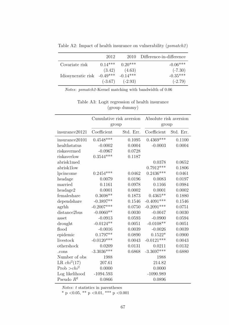
Table A2: Impact of health insurance on vulnerability (psmatch2 )

2012 2010 Difference-in-difference

Covariate risk 0.14*** 0.20*** -0.06***(3.42) (4.63) (-7.30)

Idiosyncratic risk -0.49*** -0.14*** -0.35***(-3.67) (-2.93) (-2.79)

Notes: psmatch2 -Kernel matching with bandwidth of 0.06

Table A3: Logit regression of health insurance(group dummy)

Cumulative risk aversion Absolute risk aversiongroup group

insurance20121 Coefficient Std. Err. Coefficient Std. Err.

insurance20101 0.4548*** 0.1095 0.4369*** 0.1100healthstatus -0.0002 0.0004 -0.0003 0.0004riskavermed -0.0967 0.0728riskaverlow 0.3544*** 0.1187abrisk1med 0.0378 0.0652abrisk1low 0.7912*** 0.1806lpcincome 0.2454*** 0.0462 0.2436*** 0.0461headage 0.0079 0.0196 0.0083 0.0197married 0.1161 0.0978 0.1166 0.0984headage2 0.0001 0.0002 0.0001 0.0002femaleshare 0.3698** 0.1873 0.4365** 0.1880dependshare -0.3897** 0.1546 -0.4091*** 0.1546agrhh -0.2007*** 0.0750 -0.2091*** 0.0751distance2bus -0.0060** 0.0030 -0.0047 0.0030asset -0.0913 0.0593 -0.0900 0.0594drought -0.0124** 0.0051 -0.0108** 0.0051flood -0.0016 0.0039 -0.0026 0.0039epidemic 0.1797** 0.0890 0.1522* 0.0900livestock -0.0120*** 0.0043 -0.0121*** 0.0043othershock 0.0209 0.0131 0.0211 0.0132cons -3.3036*** 0.6868 -3.3697*** 0.6880

Number of obs 1988 1988LR chi2(17) 207.61 214.82Prob >chi2 0.0000 0.0000Log likelihood -1094.593 -1090.989Pseudo R2 0.0866 0.0896

Notes: t statistics in parentheses* p <0.05, ** p <0.01, *** p <0.001

67

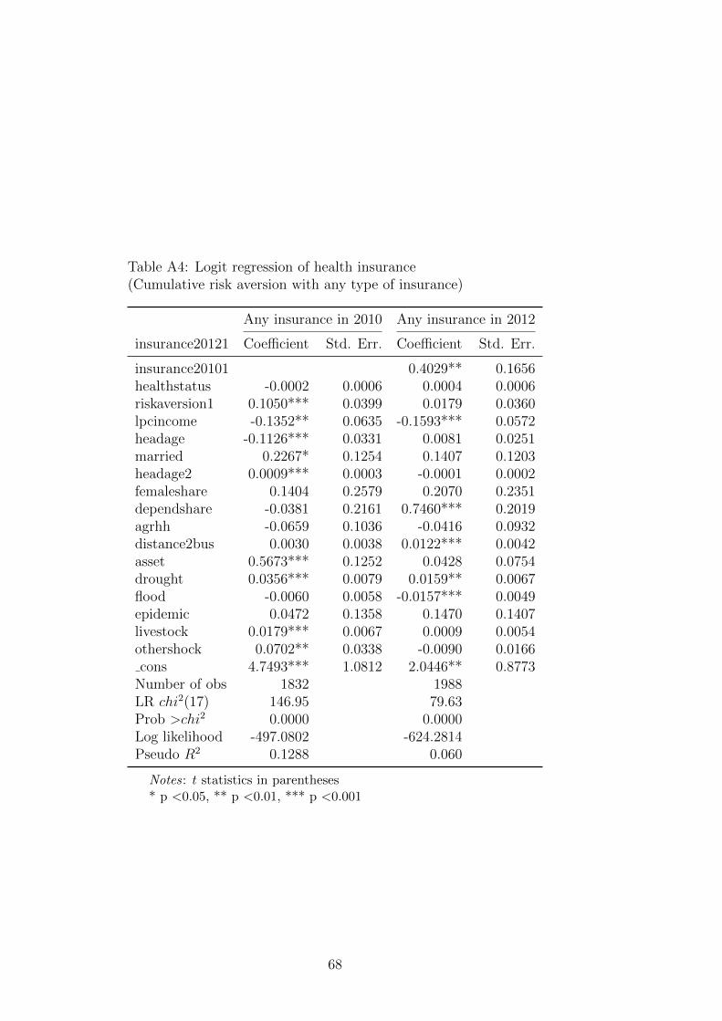
Table A4: Logit regression of health insurance(Cumulative risk aversion with any type of insurance)

Any insurance in 2010 Any insurance in 2012

insurance20121 Coefficient Std. Err. Coefficient Std. Err.

insurance20101 0.4029** 0.1656healthstatus -0.0002 0.0006 0.0004 0.0006riskaversion1 0.1050*** 0.0399 0.0179 0.0360lpcincome -0.1352** 0.0635 -0.1593*** 0.0572headage -0.1126*** 0.0331 0.0081 0.0251married 0.2267* 0.1254 0.1407 0.1203headage2 0.0009*** 0.0003 -0.0001 0.0002femaleshare 0.1404 0.2579 0.2070 0.2351dependshare -0.0381 0.2161 0.7460*** 0.2019agrhh -0.0659 0.1036 -0.0416 0.0932distance2bus 0.0030 0.0038 0.0122*** 0.0042asset 0.5673*** 0.1252 0.0428 0.0754drought 0.0356*** 0.0079 0.0159** 0.0067flood -0.0060 0.0058 -0.0157*** 0.0049epidemic 0.0472 0.1358 0.1470 0.1407livestock 0.0179*** 0.0067 0.0009 0.0054othershock 0.0702** 0.0338 -0.0090 0.0166cons 4.7493*** 1.0812 2.0446** 0.8773

Number of obs 1832 1988LR chi2(17) 146.95 79.63Prob >chi2 0.0000 0.0000Log likelihood -497.0802 -624.2814Pseudo R2 0.1288 0.060

Notes: t statistics in parentheses* p <0.05, ** p <0.01, *** p <0.001

68

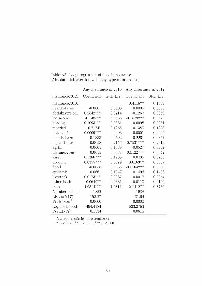
Table A5: Logit regression of health insurance(Absolute risk aversion with any type of insurance)

Any insurance in 2010 Any insurance in 2012

insurance20121 Coefficient Std. Err. Coefficient Std. Err.

insurance20101 0.4116** 0.1659healthstatus -0.0001 0.0006 0.0005 0.0006abriskaversion1 0.2542*** 0.0714 -0.1267 0.0869lpcincome -0.1485** 0.0636 -0.1579*** 0.0573headage -0.1093*** 0.0331 0.0098 0.0251married 0.2174* 0.1255 0.1380 0.1203headage2 0.0009*** 0.0003 -0.0001 0.0002femaleshare 0.1333 0.2592 0.2261 0.2357dependshare 0.0058 0.2156 0.7531*** 0.2019agrhh -0.0605 0.1039 -0.0527 0.0932distance2bus 0.0015 0.0038 0.0122*** 0.0042asset 0.5386*** 0.1236 0.0435 0.0756drought 0.0355*** 0.0079 0.0163** 0.0067flood -0.0058 0.0058 -0.0164*** 0.0050epidemic 0.0661 0.1347 0.1496 0.1408livestock 0.0173*** 0.0067 0.0017 0.0054othershock 0.0649** 0.0331 -0.0110 0.0166cons 4.9514*** 1.0811 2.1412** 0.8736

Number of obs 1832 1988LR chi2(17) 152.27 81.64Prob >chi2 0.0000 0.0000Log likelihood -494.4184 -623.2763Pseudo R2 0.1334 0.0615

Notes: t statistics in parentheses* p <0.05, ** p <0.01, *** p <0.001

69

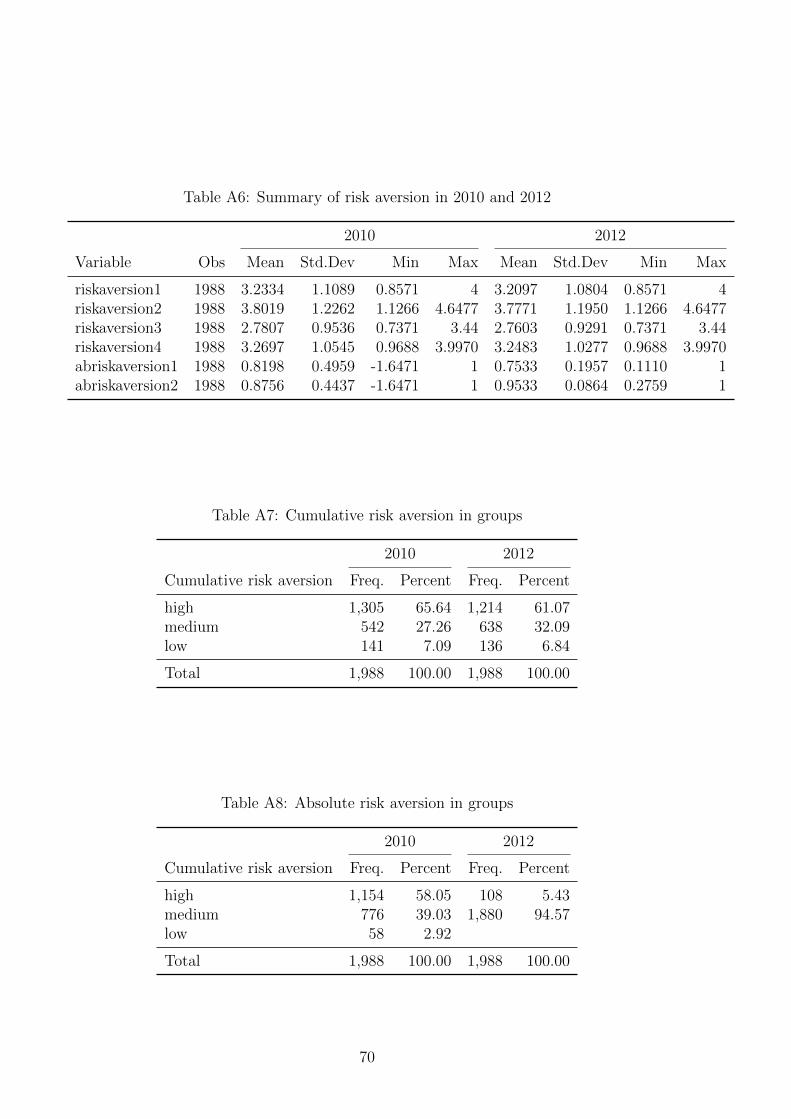
Table A6: Summary of risk aversion in 2010 and 2012

2010 2012

Variable Obs Mean Std.Dev Min Max Mean Std.Dev Min Max

riskaversion1 1988 3.2334 1.1089 0.8571 4 3.2097 1.0804 0.8571 4riskaversion2 1988 3.8019 1.2262 1.1266 4.6477 3.7771 1.1950 1.1266 4.6477riskaversion3 1988 2.7807 0.9536 0.7371 3.44 2.7603 0.9291 0.7371 3.44riskaversion4 1988 3.2697 1.0545 0.9688 3.9970 3.2483 1.0277 0.9688 3.9970abriskaversion1 1988 0.8198 0.4959 -1.6471 1 0.7533 0.1957 0.1110 1abriskaversion2 1988 0.8756 0.4437 -1.6471 1 0.9533 0.0864 0.2759 1

Table A7: Cumulative risk aversion in groups

2010 2012

Cumulative risk aversion Freq. Percent Freq. Percent

high 1,305 65.64 1,214 61.07medium 542 27.26 638 32.09low 141 7.09 136 6.84

Total 1,988 100.00 1,988 100.00

Table A8: Absolute risk aversion in groups

2010 2012

Cumulative risk aversion Freq. Percent Freq. Percent

high 1,154 58.05 108 5.43medium 776 39.03 1,880 94.57low 58 2.92

Total 1,988 100.00 1,988 100.00

70

Table A9: Pairwise correlation of risk parameters in 2010

Variable riskaver1 riskaver2 riskaver3 riskaver4 abriskaver1 abriskaver2

riskaversion1 1riskaversion2 1.0000* 1riskaversion3 1.0000* 1.0000* 1riskaversion4 1.0000* 1.0000* 1.0000* 1abriskaversion1 0.3349* 0.3339* 0.3339* 0.3339* 1abriskaversion2 0.2552* 0.2560* 0.2552* 0.2560* 0.7104* 1

Notes: * Statistically significant at 5 percent.

Table A10: Impact of health insurance coverage on idiosyncratic VEU(total health insurances across surveys, cumulative)

Random Between Random Betweeneffect variation effect variation

Health insurance -0.273*** -0.269*** -0.213*** -0.235**(total insurances across surveys) (0.045) (0.080) (0.057) (0.084)Cumulative risk aversion -0.007 0.011 -0.002 -0.005

(0.026) (0.053) (0.027) (0.054)Health status -0.029 -0.009 -0.070 -0.066

(0.034) (0.066) (0.061) (0.066)Per capita income -0.242*** -0.252*** -0.162*** -0.165**

(0.056) (0.060) (0.043) (0.066)Household characteristics No No Yes YesCommune characteristics No No Yes Yes

N 3952 3952 3952 3952R2 0.018 0.065F 9.221 5.943p 0.000 0.000 0.000 0.000

Notes: Standard errors in parentheses* p <0.05, ** p <0.01, *** p <0.001

71

Table A11: Impact of health insurance coverage on idiosyncratic VEU(health insurance at the time of interview, cumulative)

Random Between Random Betweeneffect variation effect variation

Health insurance -0.259*** -0.559*** -0.234*** -0.486**(Yes/No at the time of interview) (0.043) (0.160) (0.070) (0.167)Cumulative risk aversion -0.009 0.011 -0.003 -0.005

(0.026) (0.053) (0.027) (0.054)Health status -0.030 -0.010 -0.068 -0.067

(0.034) (0.066) (0.060) (0.066)Per capita income -0.272*** -0.251*** -0.175*** -0.165**

(0.058) (0.060) (0.045) (0.066)Household characteristics No No Yes YesCommune characteristics No No Yes Yes

N 3952 3952 3952 3952R2 0.019 0.065F 9.472 5.972p 0.000 0.000 0.000 0.000

Notes: Standard errors in parentheses* p <0.05, ** p <0.01, *** p <0.001

72

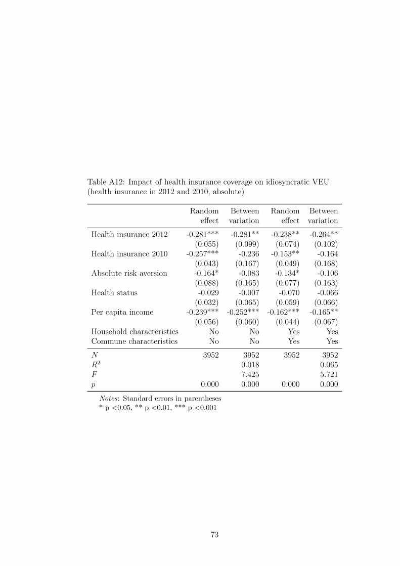
Table A12: Impact of health insurance coverage on idiosyncratic VEU(health insurance in 2012 and 2010, absolute)

Random Between Random Betweeneffect variation effect variation

Health insurance 2012 -0.281*** -0.281** -0.238** -0.264**(0.055) (0.099) (0.074) (0.102)

Health insurance 2010 -0.257*** -0.236 -0.153** -0.164(0.043) (0.167) (0.049) (0.168)

Absolute risk aversion -0.164* -0.083 -0.134* -0.106(0.088) (0.165) (0.077) (0.163)

Health status -0.029 -0.007 -0.070 -0.066(0.032) (0.065) (0.059) (0.066)

Per capita income -0.239*** -0.252*** -0.162*** -0.165**(0.056) (0.060) (0.044) (0.067)

Household characteristics No No Yes YesCommune characteristics No No Yes Yes

N 3952 3952 3952 3952R2 0.018 0.065F 7.425 5.721p 0.000 0.000 0.000 0.000

Notes: Standard errors in parentheses* p <0.05, ** p <0.01, *** p <0.001

73