Risk and Return in Fixed-Income Arbitrage: Nickels in ...jd10/nickelsRFS.pdf · Risk and Return in Fixed-Income Arbitrage: Nickels in Front of a Steamroller? Jefferson Duarte University

Risk and Return in Fixed-Income Arbitrage:

Nickels in Front of a Steamroller?

Jefferson Duarte

University of Washington

Francis A. Longstaff

UCLA Anderson School and the NBER

Fan Yu

UC Irvine

We conduct an analysis of the risk and return characteristics of a number of widely

used fixed-income arbitrage strategies. We find that the strategies requiring more

‘‘intellectual capital’’ to implement tend to produce significant alphas after controlling

for bond and equity market risk factors. These positive alphas remain significant even

after taking into account typical hedge fund fees. In contrast with other hedge fund

strategies, many of the fixed-income arbitrage strategies produce positively skewed

returns. These results suggest that there may be more economic substance to fixed-

income arbitrage than simply ‘‘picking up nickels in front of a steamroller.’’

During the hedge fund crisis of 1998, market participants were given a

revealing glimpse into the proprietary trading strategies used by a number

of large hedge funds such as Long-Term Capital Management (LTCM).

Among these strategies, few were as widely used—or as painful—as fixed-

income arbitrage. Virtually every major investment banking firm on Wall

Street reported losses directly related to their positions in fixed-incomearbitrage during the crisis. Despite these losses, however, fixed-income

arbitrage has since become one of the most popular and rapidly growing

sectors within the hedge fund industry. For example, the Tremont/TASS

(2005) Asset Flows Report indicates that total assets devoted to fixed-income

arbitrage grew by more than $9.0 billion during 2005 and that the total

We are grateful for valuable comments and assistance from Vineer Bhansali, Charles Cao, Darrell Duffie,Robert Jarrow, Philippe Jorion, Katie Kong, Haitao Li, Ravit Mandell, Bruno Miranda, Yoshihiro Mikami,Soetojo Tanudjaja, Abraham Thomas, Stuart Turnbull, Rossen Valkanov, Ryoichi Yamabe, ToshiYotsuzuka, Eric Zivot, Gary Zhu, and seminar participants at the Bank of Canada, Case Western ReserveUniversity, the Chicago Quantitative Alliance, the University of Kansas, the London School of Business,Nomura Securities, Simplex Asset Management, Pennsylvania State University, PIMCO, and the Workshopon Capital Structure Arbitrage at the University of Evry. We are particularly grateful for the comments andsuggestions of Jun Liu, the Editor Yacine Aıt-Sahalia, and of an anonymous referee. All errors are ourresponsibility. Address correspondence to: Francis Longstaff, Anderson School at UCLA, 110 WestwoodPlaza, Los Angeles, CA 90095-1481, or e-mail: [email protected].

� The Author 2006. Published by Oxford University Press on behalf of The Society for Financial Studies. All rights

reserved. For permissions, please email: [email protected].

doi:10.1093/rfs/hhl026 Advance Access publication July 6, 2006

amount of hedge fund capital devoted to fixed income arbitrage at the end of

2005 is in excess of $56.6 billion.1

This mixed history raises a number of important issues about the

fundamental nature of fixed-income arbitrage. Is fixed-income arbitrage

truly arbitrage? Or is it merely a strategy that earns small positive returns

most of the time, but occasionally experiences dramatic losses (a strategy

often described as ‘‘picking up nickels in front of a steamroller’’)? Were

the large fixed-income arbitrage losses during the hedge fund crisis simplydue to excessive leverage, or were there deeper reasons arising from the

inherent nature of these strategies? To address these issues, this article

conducts an extensive analysis of the risk and return characteristics of

fixed-income arbitrage.

Fixed-income arbitrage is actually a broad set of market-neutral invest-

ment strategies intended to exploit valuation differences between various

fixed-income securities or contracts. In this analysis, we focus on five of

the most widely used fixed-income arbitrage strategies in the market:

. Swap spread (SS) arbitrage.

. Yield curve (YC) arbitrage.

. Mortgage (MA) arbitrage.

. Volatility (VA) arbitrage.

. Capital structure (CS) arbitrage.

As in Mitchell and Pulvino (2001), our approach consists of following

specific trading strategies through time and studying the properties of

return indexes generated by these strategies. There are several important

advantages to this approach. First, it allows us to incorporate transaction

costs and hold fixed the effects of leverage in the analysis. Second, itallows us to study returns over a much longer horizon than would be

possible using the limited amount of hedge fund return data available.

Finally, this approach allows us to avoid potentially serious backfill and

survivorship biases in reported hedge fund return indexes.

With these return indexes, we can directly explore the risk and return

characteristics of the individual fixed-income arbitrage strategies. To hold

fixed the effects of leverage on the analysis, we adjust the amount of initial

capital so that the annualized volatility of each strategy’s returns is 10%.We find that all five of the strategies generate positive excess returns on

average. Surprisingly, most of the arbitrage strategies result in excess

returns that are positively skewed. Thus, even though these strategies

produce large negative returns from time to time, the strategies tend to

generate even larger offsetting positive returns.

1 The total amount of capital devoted to fixed-income arbitrage is likely much larger as the Tremont/TASS(2005) report covers less than 50% of the total estimated amount of capital managed by hedge funds.Also, many Wall Street firms directly engage in proprietary fixed-income arbitrage trading.

The Review of Financial Studies / v 20 n 3 2007

770

We study the extent to which these positive excess returns represent

compensation for bearing market risk. After risk adjusting for both

equity and bond market factors, we find that the SS and VA arbitrage

strategies produce insignificant alphas. In contrast, the YC, MA, and CS

arbitrage strategies generally result in significant positive alphas. Inter-

estingly, the latter strategies are the ones that require the most ‘‘intellec-

tual capital’’ to implement. Specifically, the strategies that result in

significant alphas are those that require relatively complex models toidentify arbitrage opportunities and/or hedge out systematic market

risks. We find that several of these ‘‘market-neutral’’ arbitrage strategies

actually expose the investor to substantial levels of market risk. We repeat

the analysis using actual fixed-income arbitrage hedge fund index return

data from industry sources and find similar results.

In addition to the transaction costs incurred in executing fixed-income

arbitrage strategies, many investors must also pay hedge fund fees. We

repeat the analysis assuming that hedge fund fees of 2/20 (a 2% manage-ment fee and a 20% slope above a Libor high water mark) are subtracted

from the returns. While these fees reduce or eliminate the significance of

the alphas of the individual strategies, we find that equally-weighted

portfolios of the more ‘‘intellectual capital’’ intensive strategies still have

significant alphas on a net-of-fees basis. On the other hand, however, our

results indicate that fees in the fixed-income arbitrage hedge fund industry

are ‘‘large’’ relative to the alphas that can be generated by these strategies.

Where does this leave us? Is the business of fixed-income arbitragesimply a strategy of ‘‘picking up nickels in front of a steamroller,’’ equiva-

lent to writing deep out-of-the-money puts? We find little evidence of this.

In contrast, we find that most of the strategies we consider result in excess

returns that are positively skewed, even though large negative returns can

and do occur. After controlling for leverage, these strategies generate

positive excess returns on average. Furthermore, after controlling for

both equity and bond market risk factors, transaction costs, and hedge

fund fees, the fixed-income arbitrage strategies that require the highestlevel of ‘‘intellectual capital’’ to implement appear to generate significant

positive alphas. The fact that a number of these factors share sensitivity to

financial market ‘‘event risk’’ argues that these positive alphas are not

merely compensation for bearing the risk of an as-yet-unrealized ‘‘peso’’

event. Thus, the risk and return characteristics of fixed-income arbitrage

appear different from those of other strategies such as merger arbitrage

[see Mitchell and Pulvino (2001)].

This article contributes to the rapidly growing literature on returns to‘‘arbitrage’’ strategies. Closest to our article are the important recent

studies of equity arbitrage strategies by Mitchell and Pulvino (2001) and

Mitchell, Pulvino, and Stafford (2002). Our article, however, focuses

exclusively on fixed-income arbitrage. Less related to our work are a

Risk and Return in Fixed-Income Arbitrage

771

number of important recent articles focusing on the actual returns reported

by hedge funds. These papers include Fung and Hsieh (1997, 2001, 2002),

Ackermann, McEnally, and Ravenscraft (1999), Brown, Goetzmann, and

Ibbotson (1999), Brown, Goetzmann, and Park (2000), Dor and Jagan-

nathan (2002), Brown and Goetzmann (2003), Getmansky, Lo, and

Makarov (2004), Agarwal and Naik (2004), Malkiel and Saha (2004),

and Chan, et al. (2005). Our article differs from these in that the returns

we study are attributable to specific strategies with controlled leverage,whereas reported hedge fund returns are generally composites of multiple

(and offsetting) strategies with varying degrees of leverage.

The remainder of this article is organized as follows. Sections 1 through

5 describe the respective fixed-income arbitrage strategies and explain

how the return indexes are constructed. Section 6 conducts an analysis

of the risk and return characteristics of the return indexes along with

those for historical fixed-income arbitrage hedge fund returns. Section 7

summarizes the results and makes concluding remarks.

1. Swap Spread Arbitrage

Swap spread arbitrage has traditionally been one of the most popular

types of fixed-income arbitrage strategies. The importance of this strategy

is evidenced by the fact that swap spread positions represented the single-

largest source of losses for LTCM.2 Furthermore, the hedge fund crisis of1998 revealed that many other major investors had similar exposure to

swap spreads—Salomon Smith Barney, Goldman Sachs, Morgan Stan-

ley, BankAmerica, Barclays, and D.E. Shaw all experienced major losses

in swap spread strategies.3

The swap spread arbitrage strategy has two legs. First, an arbitrageur

enters into a par swap and receives a fixed coupon rate CMS and pays the

floating Libor rate Lt. Second, the arbitrageur shorts a par Treasury

bond with the same maturity as the swap and invests the proceeds in amargin account earning the repo rate. The cash flows from the second leg

consist of paying the fixed coupon rate of the Treasury bond CMT and

receiving the repo rate from the margin account rt.4 Combining the cash

flows from the two legs shows that the arbitrageur receives a fixed annuity

of SS=CMS–CMT and pays the floating spread St=Lt–rt. The cash flows

from the reverse strategy are just the opposite of these cash flows. There

are no initial or terminal principal cash flows in this strategy.

2 Lowenstein (2000) reports that LTCM lost $1.6 billion in its swap spread positions before its collapse.Also see Perold (1999).

3 See Siconolfi et al. (1998), Beckett and Pacelle (1998), Dunbar (2000), and Lowenstein (2000).

4 The terms CMS and CMT are widely used industry abbreviations for constant maturity swap rate andconstant maturity Treasury rate.


772

Swap spread arbitrage is thus a simple bet on whether the fixed annuity of

SS received will be larger than the floating spread St paid. If SS is larger

than the average value of St during the life of the strategy, the strategy is

profitable (at least in an accounting sense). What makes the strategy

attractive to hedge funds is that the floating spread St has historically

been very stable over time, averaging 26.8 basis points with a standard

deviation of only 13.3 basis points during the past 16 years. Thus, the

expected average value of the floating spread over, say, a five-year horizonmay have a standard deviation of only a few basis points (and, in fact, is

often viewed as essentially constant by market participants).

Swap spread arbitrage, of course, is not actually an arbitrage in the text-

book sense because the arbitrageur is exposed to indirect default risk. This is

because if the viability of a number of major banks were to become

uncertain, market Libor rates would likely increase significantly. For

example, the spread between bank CD rates and Treasury bill yields spiked

to nearly 500 basis points around the time of the Oil Embargo during 1974.In this situation, a swap spread arbitrageur paying Libor on a swap would

suffer large negative cash flows from the strategy as the Libor rate

responded to increased default risk in the financial sector. Note that there

is no direct default risk from banks entering into financial distress as the

cash flows on a swap are not direct obligations of the banks quoting Libor

rates. Thus, even if these banks default on their debt, the counterparties to

a swap continue to exchange fixed for floating cash flows.5

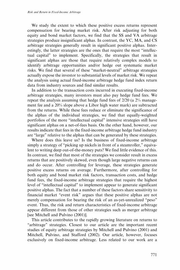
In studying the returns from fixed-income arbitrage, we use an exten-sive data set from the swap and Treasury markets covering the period

from November 1988 to December 2004. The swap data consist of

month-end observations of the three-month Libor rate and midmarket

swap rates for two-, three-, five-, seven-, and 10-year maturity swaps. The

Treasury data consist of month-end observations of the constant maturity

Treasury (CMT) rates published by the Federal Reserve in the H-15

release for maturities of two, three, five, seven, and 10 years. Finally, we

collect data on three-month general collateral repo rates. The data aredescribed in the Appendix. Figure 1 plots the time series of swap spreads

against the expected average value of the short term spread over the life of

the swap (based on fitting a simple mean reverting Gaussian process to

the data).

To construct a return index, we first determine each month whether the curr-

ent swap spread differs from the current value of the short term spread. If the

5 In theory, there is the risk of a default by a counterparty. In practice, however, this risk is negligible asswaps are usually fully collateralized under master swap agreements between major institutional inves-tors. Furthermore, the actual default exposure in a swap is far less than for a corporate bond as notionalamounts are not exchanged. Following Duffie and Huang (1996), Duffie and Singleton (1997), Minton(1997), He (2000), Grinblatt (2001), Liu, Longstaff, and Mandell (2004), and many others, we abstractfrom the issue of counterparty credit risk in this analysis.


773

difference exceeds a trigger value of 10 basis points, we implement the trade

for a $100 notional position (receive fixed on a $100 notional swap, short a

$100 notional Treasury bond, or vice versa if the difference is less than �10

basis points).6 If the difference does not exceed the trigger, then the strategy

invests in cash and earns an excess return of zero. We keep the trade on until

it converges (swap spread converges to the short term spread) or until the

maturity of the swap and bond. It is useful to think of this trade as afictional hedge fund that has only a single trade. After the first month of

the sample period, there could be one such hedge fund. After two months,

there could be two hedge funds (if neither converges), etc. Each month, we

calculate the return for each of these funds and then take the equally

weighted average across funds as the index return for that month.

In initiating and terminating positions, realistic transaction costs are

applied (described in the Appendix). As with all strategies considered in

Two-Year

0

20

40

60

80

100

120

140D

ec-8

8

Dec

-90

Dec

-92

Dec

-94

Dec

-96

Dec

-98

Dec

-00

Dec

-02

Dec

-04

Actual Spread

Expected Average

Three-Year

0

20

40

60

80

100

120

140

Dec

-88

Dec

-90

Dec

-92

Dec

-94

Dec

-96

Dec

-98

Dec

-00

Dec

-02

Dec

-04

Actual Spread

Expected Average

Five-Year

0

20

40

60

80

100

120

140

Dec

-88

Dec

-90

Dec

-92

Dec

-94

Dec

-96

Dec

-98

Dec

-00

Dec

-02

Dec

-04

Actual Spread

Expected Average

Ten-Year

0

20

40

60

80

100

120

140

Dec

-88

Dec

-90

Dec

-92

Dec

-94

Dec

-96

Dec

-98

Dec

-00

Dec

-02

Dec

-04

Actual Spread

Expected Average

Figure 1Swap spreads and expected average Libor-Repo spreadsThese graphs plot the expected average value of the Libor-repo spread and the corresponding swapspread for the indicated horizons. All spreads are in basis points.

6 We also implement the strategy with trigger values of five and 20 basis points and obtain very similarresults.


774

this article, the initial amount of capital invested in the strategy is adjusted

to fix the annualized volatility of the return index at 10% (2.887% per

month). Observe that this swap spread arbitrage strategy requires nothing

in the way of complex modeling to implement. Furthermore, as we compare

current swap spread levels to current short term spread levels, there is no

look-ahead bias in the strategy.

Table 1 provides summary statistics for the excess returns from the

swap spread strategies. As shown, the mean monthly excess returns rangefrom about 0.31 to 0.55%. All these means are significant at the 10% level,

and two are significant at the 5% level. Three of the four skewness

coefficients for the returns have positive values. Also, the returns for the

strategies tend to have more kurtosis than would be the case for a normal

distribution.

We also examine the returns from forming an equally weighted (based

on notional amount) portfolio of the individual hedge fund strategies. As

each individual strategy is capitalized to have an annualized volatility of10%, the equally weighted portfolio will have smaller volatility if the

returns from the individual strategies are not perfectly correlated. As

shown, considerable diversification is obtained with the equally weighted

portfolio as its volatility is only 82% of that of the individual strategies.

The t-statistic for the returns from the equally weighted strategy is 2.78.

The Bernardo and Ledoit (2000) gain/loss ratio for this equally weighted

strategy is 1.643 and the Sharpe ratio is 0.597.7

Finally, note that the amount of capital per $100 notional amount ofthe strategy required to fix the annualized volatility at 10% varies directly

with the horizon of the strategy. This reflects the fact that the price

sensitivity of the swap and Treasury bond increases directly with the

horizon or duration of the swap and Treasury bond.

2. Yield Curve Arbitrage

Another major type of fixed-income arbitrage involves taking long and

short positions at different points along the yield curve. These yield curve

arbitrage strategies often take the form of a ‘‘butterfly’’ trade, where, for

example, an investor may go long five-year bonds and short two- and 10-

year bonds in a way that zeros out the exposure to the level and slope of

the term structure in the portfolio. Perold (1999) reports that LTCMfrequently executed these types of yield curve arbitrage trades.

While there are many different flavors of yield curve arbitrage in the market,

most share a few common elements. First, some type of analysis is applied

7 We also investigate whether the inclusion of a stop-loss limit affects the results. The stop-loss limit iswhere an individual hedge fund is terminated upon the realization of a 20% drawdown. As the volatilityof returns is normalized to 10% per year (2.887% per month), however, the stop-loss limit is almost neverreached. Thus, the results when a stop-loss limit is included are virtually identical to those reported.


775

Table 1Summary statistics for the swap spread arbitrage strategies

Strategy Swap n Capital Mean t-StatStandarddeviation Minimum Maximum Skewness Kurtosis

Rationegative

Serialcorrelation Gain/loss

Sharperatio

SS1 2 years 193 3.671 0.546 2.94 2.887 �9.801 11.552 0.449 2.454 0.326 �0.113 1.758 0.655SS2 3 years 193 5.278 0.476 3.01 2.887 �8.482 11.209 0.178 2.002 0.326 �0.269 1.629 0.571SS3 5 years 193 9.047 0.305 1.68 2.887 �10.663 10.163 �0.456 2.269 0.332 �0.135 1.372 0.366SS4 10 years 193 15.795 0.313 1.69 2.887 �10.761 10.004 0.069 2.711 0.425 �0.114 1.381 0.376

EW SS � 193 8.448 0.410 2.78 2.378 �8.569 8.439 �0.111 2.505 0.394 �0.148 1.643 0.597

This table reports the indicated summary statistics for the monthly percentage excess returns from the swap spread arbitrage strategies. Swap denotes the swap maturity used inthe strategy. The EW SS strategy consists of taking an equally weighted (based on notional amount) position each month in the individual-maturity swap spread strategies. ndenotes the number of monthly excess returns. Capital is the initial amount of capital required per $100 notional of the arbitrage strategy to give a 10% annualized standarddeviation of excess returns. The t-statistics for the means are corrected for the serial correlation of excess returns. Ratio negative is the proportion of negative excess returns.Gain/loss is the Bernardo and Ledoit (2000) gain/loss ratio for the strategy. The sample period for the strategies is from December 1988 to December 2004.

The

Review

of

Fin

ancia

lS

tudies

/v

20

n3

2007

77

6

to identify points along the yield curve, which are either ‘‘rich’’ or ‘‘cheap.’’

Second, the investor enters into a portfolio that exploits these perceived

misvaluations by going long and short bonds in a way that minimizes the

risk of the portfolio. Finally, the portfolio is held until the trade converges and

the relative values of the bonds come back into line.

Our approach in implementing this strategy is very similar to that

followed by a number of large fixed-income arbitrage hedge funds. Spe-

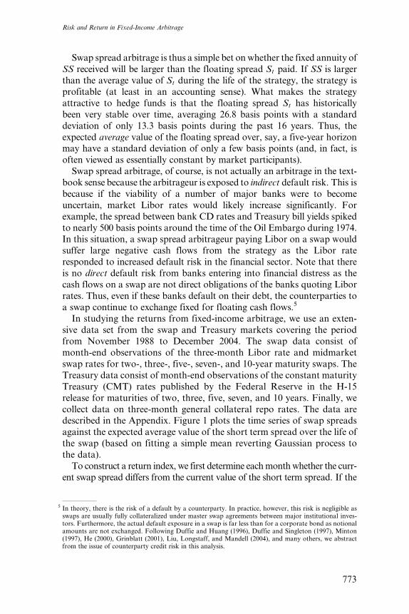
cifically, we assume that the term structure is determined by a two-factoraffine model. Using the same monthly swap market data as in the pre-

vious section, we fit the model to match exactly the one-year and 10-year

points along the swap curve each month. Once fitted to these points, we

then identify how far off the fitted curve the other swap rates are. Figure 2

graphs the time series of deviations between market and model for the

two-year, three-year, five-year, and seven-year swap rates. For example,

imagine that for a particular month, the market two-year swap rate is

more than 10 basis points above the fitted two-year swap rate. We would

Two-Year

-40

-30

-20

-10

0

10

20

30

40

Dec

-88

Dec

-90

Dec

-92

Dec

-94

Dec

-96

Dec

-98

Dec

-00

Dec

-02

Dec

-04

Three-Year

-40

-30

-20

-10

0

10

20

30

40

Dec

-88

Dec

-90

Dec

-92

Dec

-94

Dec

-96

Dec

-98

Dec

-00

Dec

-02

Dec

-04

Five-Year

-40

-30

-20

-10

0

10

20

30

40

Dec

-88

Dec

-90

Dec

-92

Dec

-94

Dec

-96

Dec

-98

Dec

-00

Dec

-02

Dec

-04

Seven-Year

-40

-30

-20

-10

0

10

20

30

40

Dec

-88

Dec

-90

Dec

-92

Dec

-94

Dec

-96

Dec

-98

Dec

-00

Dec

-02

Dec

-04

Figure 2Deviations between market and model swap ratesThese graphs plot the difference between the market swap rates for the indicated horizons and thecorresponding values implied by the two-factor affine model fitted to match exactly the one-year and10-year swap rates. All deviations are in basis points.


777

enter into a trade by going long (receiving fixed) $100 notional of a two-

year swap and going short a portfolio of one-year and 10-year swaps with

the same sensitivity to the two affine factors as the two-year swap. Thus,

the resulting portfolio’s sensitivity to each of the two factors would be

zero. Once this butterfly trade was put on, it would be held for 12 months

or until the market two-year swap rate converged to the model value. The

same process continues for each month, with either a trade similar to the

above, the reverse trade of the above, or no trade at all being implemented(in which case the strategy invests in cash and earns zero excess return),

and similarly for the other swap maturities. Unlike the swap spread

strategy of the previous section, this strategy involves a high degree of

‘‘intellectual capital’’ to implement as both the process of identifying

arbitrage opportunities and the associated hedging strategies require the

application of a multi-factor term structure model.

As before, we can think of a butterfly trade put on in a specific month as

a fictional hedge fund with only one trade. Similarly, we can compute thereturn on this hedge fund until the trade converges. For a given month,

there may be a number of these hedge funds, each representing a trade that

was put on previously but has not yet converged. The return index for the

strategy for a given month is the equally weighted average of the returns for

all the individual hedge funds active during that month. As in the previous

section, we include realistic transaction costs in computing returns and

adjust the capital to give an annualized volatility of 10% for the index

returns. The details of the strategy are described in the Appendix.8

Table 2 reports summary statistics for the excess returns from the yield

curve strategies. We use a trigger value of 10 basis points in determining

whether to implement a trade.9 We implement the strategy separately for

two-year, three-year, five-year, and seven-year swaps and also implement

an equally weighted strategy (in terms of notional amount) of the indivi-

dual-horizon strategies. As shown, the average monthly excess returns

from the individual strategies as well as for the equally weighted strategy

are all statistically significant and range from about 0.4 to 0.6%.Table 2 also summarizes that the excess returns are highly positively

skewed. The positive skewness of the returns argues against the view that

this strategy is one in which an arbitrageur earns small profits most of the

time but occasionally suffers a huge loss. As before, the excess returns

display more kurtosis than would be the case for a normal distribution.

8 At each date, we fit the model to match exactly the current one- and 10-year swaps. Thus, there is nolook-ahead bias in the state variables of the model. While the parameters of the model are estimated overthe entire sample, however, they are used only in determining the hedge ratios for butterfly trades. Thus,there should be little or no look-ahead bias in the results. As a diagnostic, we estimated the model usingdata for the first part of the sample period and then applied it to strategies for the latter part of thesample. The results from this exercise are virtually identical to those we report.

9 Using a trigger value of five basis points gives similar results.


778

Table 2Summary statistics for the yield curve arbitrage strategies

Strategy Swap n Capital Mean t-StatStandarddeviation Minimum Maximum Skewness Kurtosis

Rationegative


Sharperatio

YC1 2 years 193 4.847 0.540 2.76 2.887 �6.878 10.056 0.569 0.902 0.301 �0.059 1.770 0.648YC2 3 years 193 7.891 0.486 2.31 2.887 �6.365 11.558 0.591 1.172 0.337 0.014 1.643 0.583YC3 5 years 193 7.794 0.615 3.29 2.887 �8.307 11.464 0.592 2.366 0.212 �0.108 2.102 0.738YC4 7 years 193 4.546 0.437 2.46 2.887 �10.306 20.032 2.156 14.953 0.088 �0.158 2.355 0.524

EW YC � 193 6.270 0.519 3.42 2.293 �5.241 11.329 0.995 3.269 0.347 �0.084 1.980 0.785

This table reports the indicated summary statistics for the monthly percentage excess returns from the yield curve arbitrage strategies. Swap denotes the swap maturity used inthe strategy. The EW YC strategy consists of taking an equally weighted (based on notional amount) position each month in the individual-maturity yield curve strategies. ndenotes the number of monthly excess returns. Capital is the initial amount of capital required per $100 notional of the arbitrage strategy to give a 10% annualized standarddeviation of excess returns. The t-statistics for the means are corrected for the serial correlation of excess returns. Ratio negative is the proportion of negative excess returns.Gain/loss is the Bernardo and Ledoit (2000) gain/loss ratio for the strategy. The sample period for the strategies is from December 1988 to December 2004.

Risk

and

Retu

rnin

Fix

ed-In

com

eA

rbitra

ge

77

9

Finally, observe that the amount of capital required to attain a 10% level

of volatility is typically much less than in the swap spread strategies. This

reflects the fact that the yield curve trade tends to be better hedged as all

the positions are along the same curve, and the factor risk is neutralized in

the portfolio.

3. Mortgage Arbitrage

The mortgage-backed security (MBS) strategy consists of buying MBS

passthroughs and hedging their interest rate exposure with swaps. A

passthrough is a MBS that passes all the interest and principal cash

flows of a pool of mortgages (after servicing and guarantee fees) to the

passthrough investors. MBS passthroughs are the most common type ofmortgage-related product and this strategy is commonly implemented by

hedge funds. The Bond Market Association indicates that MBS now

forms the largest fixed-income sector in the U.S.

The main risk of a MBS passthrough is prepayment risk. That is, the timing

of the cash flows of a passthrough is uncertain because homeowners have the

option to prepay their mortgages.10 The prepayment option embedded in

MBS passthroughs generates the so-called negative convexity of these secu-

rities. For instance, the top panel of Figure 3 plots the nonparametricestimate of the price of a generic Ginnie Mae (GNMA) passthrough with

a 7% coupon rate as a function of the five-year swap rate (see the Appendix

for details on the estimation procedure, data, and strategy implementation).

It is clear that the price of this passthrough is a concave function of the

interest rate. This negative convexity arises because homeowners refinance

their mortgages as interest rates drop, and the price of a passthrough

consequently converges to some level close to its principal amount.

A MBS portfolio duration hedged with swaps inherits the negative con-vexity of the passthroughs. For example, the bottom panel of Figure 3 plots

the value of a portfolio composed of a $100 notional long position in a

generic 7% GNMA passthrough, duration hedged with the appropriate

amount of a five-year swap. This figure reveals that abrupt changes in

interest rates will cause losses in this portfolio. To compensate for these

possible losses, investors require higher yields to hold these securities. Indeed,

Bloomberg’s option-adjusted spread (OAS) for a generic 7% GNMA pass-

through during the period from November 1996 to February 2005 wasbetween 48 and 194 basis points with a mean value of 112 basis points.11

10 For discussions about the effects of prepayment on MBS prices, see Dunn and McConnell (1981a,b),Schwartz and Torous (1989, 1992), Stanton (1995), Boudoukh et al. (1997), and Longstaff (2005).

11 OASs are commonly used as a way of analyzing the relative valuations of different MBSs. As opposed tostatic spreads, the OAS incorporates the information about the timing of the cash flows of a passthroughwith the use of a prepayment model and a term structure model in its calculation. The OAS thereforeadjusts for the optionality of a passthrough. For a discussion of the role of OAS in the MBS market, seeGabaix, Krishnamurthy, and Vigneron (2004).


780

Long positions in passthroughs are usually financed with a form of

repurchase agreement called a dollar roll. Dollar rolls are analogous to

standard repurchase agreements in the sense that a hedge fund entering

into a dollar roll sells a passthrough to a MBS dealer and agrees to buy

back a similar security in the future at a predetermined price. The main

difference between a standard repurchase agreement and a dollar roll is

that with the roll, the dealer does not have to deliver a passthrough backedby exactly the same pool of mortgages. Unlike traditional repurchase

agreements, a dollar roll does not require any haircut or over-collateraliza-

tion [see Biby, Modukuri, and Hargrave (2001)]. Dealers extend favorable

financing terms because dollar rolls give them the flexibility to

manage their MBS portfolios. Assume, for instance, that a MBS dealer

85

90

95

100

105

110

2.0 3.0 4.0 5.0 6.0 7.0 8.0 9.0

Five-Year Swap Rate

Pas

sthr

ough

Pri

ce

90

92

94

96

98

100

102

2.0 3.0 4.0 5.0 6.0 7.0 8.0 9.0

Five-Year Swap Rate

Hed

ged

Por

tfol

io V

alue

Figure 3Passthrough price as a function of swap ratesThe top panel of this figure displays the nonparametric estimate of the price of the 7% GNMApassthrough as a function of the five-year swap rate. Each point in this figure represents 25 dailyobservations. The bottom panel displays the value of a portfolio with $100 notional amount of thispassthrough duration-hedge with a five-year swap. The hedge is initiated when the swap rate is 6.06%.


781

wishes to cover an existing short position in the MBS market. To do so,

the dealer can buy a passthrough from a hedge fund with the dollar roll.

At the end of the roll term, the dealer does not need to return a

passthrough backed by exactly the same pool of mortgages. As a result,

dollar rolls can be used as a mechanism to cover short positions in the

passthrough market.

The overall logic of the strategy of buying MBS passthroughs, financing

them with dollar rolls, and hedging their duration with swaps is thereforetwo-fold. First, investors require larger yields to carry the negative con-

vexity of MBS passthroughs. Second, the delivery option of the dollar rolls

makes them a cheap source of MBS financing. To execute the strategy, it is

necessary to specify which agency passthroughs are used [Ginnie Mae

(GNMA), Fannie Mae (FNMA), or Freddie Mac (FHLMC)], the MBS

coupons (trading at discount or at premium), the swap maturities used in

the hedge, the model used to calculate the hedge ratios, the frequency of

hedge rebalancing (daily, weekly or monthly), and the OAS level abovewhich a long position in the passthrough is taken (the OAS trade trigger).

We use GNMA passthroughs because they are fully guaranteed by the

U. S. Government and are consequently free of default risk.12 The pass-

throughs we study are those with coupons closest to the current coupon

as they are the most liquid. The passthroughs are hedged with five-year

swaps. There is a large diversity of models that can be used to calculate

hedge ratios. Indeed, every major MBS dealer has a proprietary prepay-

ment model. Typically, these proprietary models require a high level of‘‘intellectual capital’’ to develop, maintain, and use. We expect that some

of these models used in practice deliver better hedge ratios than others.

However, we do not want to base our results on a specific parametric

model. Rather, we wish to have hedge ratios that work well on average.

To this end, we adopt a nonparametric approach to estimate the hedge

ratios. Specifically, we use the method developed by Aıt-Sahalia and

Duarte (2003) to estimate the first derivative of the passthrough price

with respect to the five-year swap rate, with the constraint that pass-through prices are a nonincreasing function of the five-year swap rate. We

use all the available sample of passthrough prices for this estimation.13

The hedging rebalancing frequency is monthly. We expect that most

hedge funds following this strategy estimate the duration of their portfo-

lios at least daily and rebalance when the duration deviates substantially

12 All the mortgage loans securitized by GNMA are federally insured. Among the guarantors are the FHAand VA.

13 Even though the model is estimated over the entire sample, the current five-year swap rate is used tospecify the hedging ratio. Thus, there is no look-ahead bias in the state variable of the model. To checkwhether look-ahead bias is induced by the parameter estimation procedure, we also estimated the modelfor the 6.5 and 7.0% coupons using only data available prior to the first day that the strategy isimplemented. The returns obtained using the hedge ratios implied by this estimation procedure arevirtually identical to those obtained when the entire sample period is used in the estimation.


782

from zero. For reasons of simplicity, we assume that all the trading in this

strategy is done on the last trading day of the month. Trade triggers based

on OAS may be used to improve the returns of mortgage strategies [see

for instance Hayre (1990)]. We, however, take a long position on MBS

passthroughs independently of their OAS as we want to avoid any depen-

dence of our results on a specific prepayment model.

The strategy is implemented between December 1996 and December 2004

with a total of 97 monthly observations. The results of this strategy aredisplayed in Table 3. The first row of Table 3 displays the results of the

strategy implemented with passthroughs trading at a discount. The second

row displays the results of holding the passthrough with coupon closest to

the current coupon, which can be trading at either a premium or a discount.

The results using the premium passthroughs with coupons closest to the

current coupons are in the third row. We again report results for an equally

weighted portfolio (in terms of notional amount) of the individual strategies.

The excess returns of the MBS strategies can be either positively skewed(discount strategy) or negatively skewed (the premium strategy). The

excess returns of the strategies are not significantly autocorrelated. The

mean excess returns of the discount and par strategies are 0.691 and

0.466%. The mean returns of the discount and par strategies are statisti-

cally significant at roughly the 10% level. The performance of the pre-

mium passthrough strategy is considerably worse than that of the other

strategies. The mean monthly return of the premium strategy is not

different from zero at usual significance levels. The relatively poor per-formance of the premium passthrough strategy is partially caused by the

strong negative convexity of the premium passthroughs. Indeed, the

passthroughs in the premium strategy have an average convexity of

�1:53 compared to �1:44 for the passthroughs in the par strategy and

�1:11 for the passthroughs in the discount strategy.

4. Fixed-Income Volatility Arbitrage

In this section, we examine the returns from following a fixed-income

volatility arbitrage strategy. Volatility arbitrage has a long tradition as a

popular and widely used strategy among Wall Street firms and other

major financial market participants. Volatility arbitrage also plays amajor role among fixed income hedge funds. For example, Lowenstein

(2000) reports that LTCM lost more than $1.3 billion in volatility arbit-

rage positions before the fund’s demise in 1998.

In its simplest form, volatility arbitrage is often implemented by selling

options and then delta-hedging the exposure to the underlying asset. In

doing this, investors hope to profit from the well-known tendency of

implied volatilities to exceed subsequent realized volatilities. If the implied

volatility is higher than the realized volatility, then selling options produces an


783

Table 3Summary statistics for the mortgage arbitrage strategies

Strategy Mortgage n Capital Mean t-StatStandarddeviation Minimum Maximum Skewness Kurtosis

Rationegative


Sharperatio

MA1 Discount 97 21.724 0.691 2.08 2.887 �6.794 11.683 0.882 2.929 0.383 0.128 1.999 0.830MA2 Par 97 19.779 0.466 1.50 2.887 �7.600 11.676 0.330 2.263 0.402 0.059 1.565 0.560MA3 Premium 97 16.910 0.065 0.23 2.887 �8.274 9.844 �0.274 1.452 0.402 �0.052 1.063 0.078

EW MA � 97 19.471 0.408 1.39 2.750 �7.556 8.539 0.064 1.027 0.392 0.053 1.489 0.514

This table reports the indicated summary statistics for the monthly percentage excess returns from the mortgage arbitrage strategies. Mortgage denotes the type of mortgage-backed securities used in the strategy—discount, par, or premium. The EW MA strategy consists of taking an equally weighted (based on notional amount) position each monthin the individual discount, par, and premium mortgage arbitrage strategies. n denotes the number of monthly excess returns. Capital is the initial amount of capital required per$100 notional of the arbitrage strategy to give a 10% annualized standard deviation of excess returns. The t-statistics for the means are corrected for the serial correlation ofexcess returns. Ratio negative is the proportion of negative excess returns. Gain/Loss is the Bernardo and Ledoit (2000) gain/loss ratio for the strategy. The sample period forthe strategies is from December 1996 to December 2004.

The

Review

of

Fin

ancia

lS

tudies

/v

20

n3

2007

78

4

excess return proportional to the gamma of the option times the difference

between the implied variance and the realized variance of the underlying

asset.14

In implementing a fixed-income volatility arbitrage strategy, we focus

on interest rate caps. Interest rate caps are among the most important and

liquid fixed-income options in the market. Interest rate caps consist of

portfolios of individual European options on the Libor rate [for example,

see Longstaff, Santa-Clara, and Schwartz (2001)]. Strategy returns, how-ever, would be similar if we focused on cap/floor straddles instead.

At-the-money caps are struck at the swap rate for the corresponding

maturity. The strategy can be thought of as selling a $100 notional

amount of at-the-money interest rate caps and delta-hedging the position

using Eurodollar futures. In actuality, however, the strategy is implemen-

ted in a slightly different way that involves a series of short-term volatility

swaps. This alternative approach is essentially the equivalent of shorting

caps but allows us to avoid a number of technicalities. The details of howthe strategy is implemented are described in the Appendix.

The data used in constructing an index of cap volatility arbitrage returns

consist of the swap market data described in Section 1, daily Eurodollar

futures closing prices obtained from the Chicago Mercantile Exchange, and

interest rate cap volatilities provided by Citigroup and the Bloomberg

system. To incorporate transaction costs, we assume that the implied

volatility at which we sell caps is 1% less than the market midpoint of

the bid-ask spread (for example, at a volatility of 17% rather than at themidmarket volatility of 18%). Because the bid-ask spread for caps is

typically less than 1% (or one vega), this gives us conservative estimates

of the returns from the strategy. The excess return for a given month can be

computed from the difference between the implied variance of a caplet at

the beginning of the month, and the realized variance for the corresponding

Eurodollar futures contracts over the month. The deltas and gammas for

the individual caplets can be calculated using the standard Black (1976)

model used to quote cap prices in this market. Although the Black model isused to compute hedge ratios, the strategy actually requires little in the way

of modeling sophistication. To see this, recall that in the Black model, the

delta of an at-the-money straddle is essentially zero. Thus, this strategy

could be implemented almost entirely without the use of a model by simply

selling cap/floor straddles over time. Note that there is no look-ahead bias

in this implementation of the strategy.

Table 4 reports summary statistics for the volatility arbitrage return indexes

based on the strategies for the highly liquid two-, three-, four-, and five-yeacap maturities as well as for the equally weighted (based on notional

14 For discussions of the relation between implied and realized volatilities, see Day and Lewis (1988),Lamoureux and Lastrape (1993), and Canina and Figlewski (1993).


785

Table 4Summary statistics for the fixed-income volatility arbitrage strategies

Strategy Cap n Capital Mean t-StatStandarddeviation Minimum Maximum Skewness Kurtosis

Rationegative


Sharperatio

VA1 2 years 183 0.734 0.389 1.11 2.887 �9.720 6.550 �0.962 1.579 0.383 0.465 1.423 0.467VA2 3 years 183 0.863 0.609 1.77 2.887 �9.675 6.851 �0.909 1.332 0.355 0.445 1.722 0.731VA3 4 years 183 0.953 0.682 2.08 2.887 �10.295 7.087 �0.989 1.644 0.311 0.409 1.823 0.819VA4 5 years 150 1.082 0.488 1.32 2.887 �9.997 6.654 �0.988 1.772 0.347 0.423 1.543 0.586

EW VA � 183 0.908 0.584 1.79 2.280 �9.592 6.674 �0.925 1.392 0.344 0.425 1.709 0.720

This table reports the indicated summary statistics for the monthly percentage excess returns from the fixed-income volatility arbitrage strategy of shorting at-the-moneyinterest rate caps of the indicated maturity. The EW VA strategy consists of taking an equally weighted (based on notional amount) position each month in the individual-maturity volatility arbitrage strategies. n denotes the number of monthly excess returns. Capital is the initial amount of capital required per $100 notional of the arbitragestrategy to give a 10% annualized standard deviation of excess returns. The t-statistics for the means are corrected for the serial correlation of excess returns. Ratio negative isthe proportion of negative excess returns. Gain/loss is the Bernardo and Ledoit (2000) gain/loss ratio for the strategy. The sample period for the strategies is from October 1989to December 2004 (but is shorter for some strategies because cap volatility data for earlier periods are unavailable).

The

Review

of

Fin

ancia

lS

tudies

/v

20

n3

2007

78

6

amount) strategy. As shown, the volatility arbitrage strategy tends to produce

positive excess returns. The average excess returns range from about 0.40 to

nearly 0.70% per month. The average excess return for the three-year cap

strategy is significant at the 10% level, and the average excess return for the

four-year cap strategy is significant at the 5% level. The average excess return

for the equally weighted strategy is also significant at the 10% level. As an

illustration of why this strategy produces positive excess returns, Figure4 graphs the implied volatility of a four-year cap against the average

(over the corresponding 15 Eurodollar futures contracts used to hedge

the cap) realized Eurodollar futures volatility (both expressed in terms

of annualized basis point volatility). In this figure, the implied volatility

clearly tends to be higher than the realized volatility. Unlike the pre-

vious strategies considered, volatility arbitrage produces excess returns

that are highly negatively skewed. In particular, the skewness coeffi-

cients for all the strategies are negative. Thus, these excess returnsappear more consistent with the notion of ‘‘picking up nickels in front

of a steamroller.’’ The excess returns again display more kurtosis than

would normally distributed random variables. These strategies require

far less capital for a $100 notional trade than the previous strategies.

5. Capital Structure Arbitrage

Capital structure arbitrage (or alternatively, credit arbitrage) refers to a class

of fixed-income trading strategies that exploit mispricing between a company’s

0

50

100

150

200

250

Dec

-89

Dec

-90

Dec

-91

Dec

-92

Dec

-93

Dec

-94

Dec

-95

Dec

-96

Dec

-97

Dec

-98

Dec

-99

Dec

-00

Dec

-01

Dec

-02

Dec

-03

Dec

-04

Implied

Realized

Figure 4Implied and realized basis point volatility of four-year interest rate capsThis graph plots the implied annualized basis point volatility for a four-year interest rate cap along withthe average annualized realized basis point volatility over the subsequent month of the Eurodollarfutures contract corresponding to the individual caplets of the cap.


787

debt and its other securities (such as equity). With the exponential growth in

the credit default swap (CDS) market in the last decade, this strategy has

become increasingly popular with proprietary trading desks at investment

banks.15 In fact, Euromoney reports that some traders describe this strategy

as the ‘‘most significant development since the invention of the CDS itself

nearly ten years ago’’ [Currie and Morris (2002)]. Furthermore, the Financial

Times reports that ‘‘hedge funds, faced with weak returns or losses on some

of their strategies, have been flocking to a new one called capital structurearbitrage, which exploits mispricings between a company’s equity and debt’’

[Skorecki (2004)].

This section implements a simple version of capital structure arbitrage

for a large cross-section of obligors. The purpose is to analyze the risk and

return of the strategy as commonly implemented in the industry. Using

the information on the equity price and the capital structure of an obligor,

we compute its theoretical CDS spread and the size of an equity position

needed to hedge changes in the value of the CDS or what is commonlyreferred to as the equity delta. We then compare the theoretical CDS

spread with the level quoted in the market. If the market spread is higher

(lower) than the theoretical spread, we short (long) the CDS contract,

while simultaneously maintaining the equity hedge. The strategy would be

profitable if, subsequent to initiating a trade, the market spread and the

theoretical spread converge to each other.

More specifically, we generate the predicted CDS spreads using the

CreditGrades (CG) model, which was jointly devised by severalinvestment banks as a market standard for evaluating the credit risk

of an obligor.16 It is loosely based on Black and Cox (1976), with

default defined as the first passage of a diffusive firm value to an

unobserved ‘‘default threshold.’’ For CDS data we use the comprehen-

sive coverage provided by the Markit Group, which consists of daily

spreads of five-year CDS contracts on North American industrial obli-

gors from 2001 to 2004. To facilitate the trading analysis, we require

that an obligor should have at least 252 daily CDS spreads no more thantwo weeks apart from each other.17 After merging firm balance sheet

data from Compustat and equity prices from Center for Research in

Security Prices (CRSP), the final sample contains 135,759 daily spreads

on 261 obligors. Details on the calibration of the model and the trading

15 CDSs are essentially insurance contracts against the default of an obligor. Specifically, the buyer of theCDS contract pays a premium each quarter, denoted as a percentage of the underlying bond’s notionalvalue in basis points. The seller agrees to pay the notional value for the bond should the obligor defaultbefore the maturity of the contract. CDSs can be used by commercial banks to protect the value of theirloan portfolios. For a more detailed description of the CDS contract, see Longstaff, Mithal, and Neis(2005).

16 For details about the model, see Finkelstein et al. (2002).

17 This criterion is consistent with capital structure arbitrageurs trading in the most liquid segment of theCDS market. On the practical side, it also yields a reasonably broad sample.


788

strategy are provided in the Appendix. This strategy clearly requires a

high level of financial knowledge to implement.

To illustrate the intuition behind the trading strategy, we present the

market spread, the theoretical spread, and the equity price for General

Motors (GM) in Figure 5. First, we observe that there is a negative

correlation between the CDS spread and the equity price. Indeed, the

correlation between changes in the equity price and the market spread for

GM is �0:32. Moreover, the market spread appears to be more volatile,reverting to the model spread over the long run. For example, the market

spread widened to over 440 basis points during October 2002, while the

model spread stayed below 300 basis points. This gap diminished shortly

thereafter and completely disappeared by February 2003. The arbitra-

geur would have profited handsomely if he were to short CDS and short

equity as a hedge during this period. Note, however, that if the arbitra-

geur placed the same trades two months earlier in August 2002, he would

have experienced losses as the CDS spread continued to diverge. Theshort equity hedge would have helped to some extent in this case, but its

effectiveness remains doubtful due to the low correlation between the

CDS spread and the equity price.

Incidentally, a similar scenario played out again in May 2005 when

GM’s debt was on the verge of being downgraded. Seeing GM’s CDS

becoming ever more expensive, many hedge funds shorted CDS on GM

and hedged their exposure by shorting GM equity. GM’s debt was indeed

downgraded shortly afterwards, but not before Kirk Kerkorianannounced a $31-per-share offer to increase his stake in GM, causing

the share price to soar. According to The Wall Street Journal, this ‘‘dealt

0

50

100

150

200

250

300

350

400

450

500

Feb

-02

May

-02

Au

g-0

2

No

v-0

2

Feb

-03

May

-03

Au

g-0

3

No

v-0

3

Feb

-04

May

-04

Au

g-0

4

No

v-0

4

CD

S Sp

read

s

0

10

20

30

40

50

60

70

80

Equ

ity

Pri

ce

Market CDS Spread

Model CDS Spread

Equity Price

Figure 5General Motors CDS spreads and equity priceThis figure displays the market CDS spread, the model CDS spread, and the equity price for GeneralMotors. The CDS spreads are in basis points.


789

the hedge funds a painful one-two punch: their debt bets lost money, and

the loss was compounded when their hedge lost out as the stock price

rose’’ [Zuckerman (2005)]. Overall, the GM experience suggests that the

risk for individual trades is typically a combination of rapidly rising

market spreads and imperfect hedging from the offsetting equity posi-

tions.

We implement the trading strategy for all obligors as follows. For each

day t in the sample period of an obligor, we check whetherct > ð1þ �Þ c¢t, where ct and c¢t are the market and model spreads, respec-

tively, and � is called the trigger level for the strategy. If this criterion is

satisfied, we short a CDS contract with a notional amount of $100 and

short an equity position as given by the CG model.18 The positions are

liquidated when the market spread and the model spread become equal,

or after 180 days, whichever occurs first. We assume a 5% bid-ask spread

for trading CDS. This is a realistic estimate of CDS market transaction

costs in recent periods.As there are 261 obligors in the final sample, we typically have thou-

sands of open trades throughout the sample period. We create the

monthly index return as follows. First, as the CDS position has an initial

value of zero, we assume that each trade is endowed with an initial level of

capital, from which the equity hedge is financed. All subsequent cash

flows, such as CDS premiums and cash dividends on the stock position,

are credited to or deducted from this initial capital. We also compute the

value of the outstanding CDS position using the CG model and obtaindaily excess returns for each trade. Then, we calculate an equally weighted

average daily return across all open trades for each day in the sample and

compound them into a monthly frequency. This yields 48 numbers that

represent monthly excess returns obtained by holding an equally weighted

portfolio of all available capital structure arbitrage trades. As all infor-

mation used in implementing the strategy is contemporaneous, there is no

look-ahead bias in strategy returns.

Table 5 summarizes the monthly excess returns for six strategies imple-mented for three trading trigger levels and for investment-grade or spec-

ulative-grade obligors. Also reported are the results for an equally

weighted portfolio (based on notional amounts). First, we notice that

the amount of initial capital required to generate a 10% annualized

standard deviation is several times larger than for any of the previous

strategies. This is an indication of the risk involved in capital structure

arbitrage. In fact, results not presented here show that convergence occurs

for only a small fraction of the individual trades. Furthermore, althoughTable 5 does not show any significant change in the risk and return of the

18 We also consider the strategy of buying CDS contracts and putting on a long equity hedge whenc¢t > ð1þ �Þ ct. This strategy yields slightly lower excess returns.


790

Table 5Summary statistics for the capital structure arbitrage strategies

Strategy Rating Trigger n Capital Mean t-StatStandarddeviation Minimum Maximum Skewness Kurtosis

Rationegative

Serialcorrelation Gain/ loss

Sharperatio

CS1 Investment 1.00 48 47.000 0.768 1.95 2.887 �8.160 10.570 0.223 5.337 0.271 �0.055 2.621 0.922CS2 1.50 48 52.300 0.613 1.25 2.887 �8.020 12.770 0.266 8.682 0.375 0.162 2.435 0.735CS3 2.00 48 44.900 0.731 1.30 2.887 �4.640 13.790 0.342 10.075 0.417 0.296 3.341 0.877

CS4 Speculative 1.00 48 86.900 0.709 2.30 2.887 �8.680 7.680 0.331 2.646 0.167 �0.298 2.513 0.851CS5 1.50 48 90.500 0.669 2.17 2.887 �7.250 10.920 0.358 4.661 0.146 �0.306 2.921 0.802CS6 2.00 48 75.900 0.740 1.03 2.887 �1.730 15.210 0.448 15.889 0.104 0.505 12.738 0.887

EW CS � � 48 66.250 0.705 1.70 2.029 �1.955 9.650 2.556 8.607 0.333 0.343 4.117 1.203

This table reports the indicated summary statistics for the monthly percentage excess returns from the capital structure arbitrage strategies. Rating denotes whether the strategyis applied to investment-grade or speculative-grade CDS obligors. Trigger denotes the ratio of the difference between the market spread and the model spread divided by themodel spread, above which the strategy is implemented. The EW CS strategy consists of taking an equally weighted (based on notional amount) position each month in theindividual capital structure arbitrage strategies. n denotes the number of monthly excess returns. Capital is the initial amount of capital required per $100 notional of thearbitrage strategy to give a 10% annualized standard deviation of excess returns. The t-statistics for the means are corrected for the serial correlation of excess returns. Rationegative is the proportion of negative excess returns. Gain/loss is the Bernardo and Ledoit gain/loss ratio for the strategy. The sample period for the strategies is from January2001 to December 2004.

Risk

and

Retu

rnin

Fix

ed-In

com

eA

rbitra

ge

79

1

strategies when the trade trigger level is increased from 1 to 2, the mean

return can in fact become 0 or negative at lower values of �, say 0.5. This

suggests that the information content of a small deviation between the

market spread and the predicted spread is low, and capital structure

arbitrage becomes profitable only when implemented at higher threshold

levels. Three of the six strategies have average monthly excess returns

that are statistically significant at the 5% level. The equally weighted

strategy has significantly lower volatility than the individual strategies,indicating that the individual strategies are not perfectly correlated with

each other. Finally, these excess returns all display positive skewness and

have more kurtosis than would a normally distributed random variable.

6. Fixed-Income Arbitrage Risk and Return

In this section, we study the risk and return characteristics of the fixed-

income arbitrage strategies. In particular, we explore whether the excess

returns generated by the strategies represent compensation for exposure

to systematic market factors.

6.1 Risk-Adjusted Returns

The five fixed-income arbitrage strategies we study are often described inhedge fund marketing materials as ‘‘market-neutral’’ strategies. For exam-

ple, as the swap spread strategy consists of a long position in a swap and

an offsetting short position in a Treasury bond with the same maturity (or

vice versa), this trade is often viewed as having no directional market risk.

In actuality, however, this strategy is subject to the risk of a major

widening in the Treasury-repo spread. Similar arguments can be directed

at each of the other arbitrage strategies we consider. If the residual risks

of these strategies are correlated with market factors, then the excessreturns reported in previous tables may in fact represent compensation

for the underlying market risk of these strategies.

To examine this issue, our approach will be to regress the excess returns

for the various strategies on the excess returns of a number of equity and

bond portfolios. For perspective, Figures 6 and 7 plot the time series of

excess returns for the equally weighted SS, YC, MA, VA, and CS strate-

gies. To control for equity-market risk, we use the excess returns for the

Fama and French (1993) market ðRMÞ, small-minus-big (SMB), high-minus-low (HML), and up-minus-down (momentum or UMD) portfo-

lios (excess returns are provided courtesy of Ken French). Also, we

include the excess returns on the S&P bank stock index (from the

Bloomberg system). To control for bond market risk, we use the excess

returns on the CRSP Fama two-year, five-year, and 10-year Treasury

bond portfolios. As controls for default risk, we also use the excess

returns for a portfolio of A/BBB-rated industrial bonds and for a


792

portfolio of A/BBB-rated bank sector bonds (provided by Merrill Lynch

and reported in the Bloomberg system). Table 6 reports the regression

results for each of the strategies, including the value of the alpha (the

Swap Spread Arbitrage

-10%

-8%

-6%

-4%

-2%

0%

2%

4%

6%

8%

10%

12%

Yield Curve Arbitrage

-10%

-8%

-6%

-4%

-2%

0%

2%

4%

6%

8%

10%

12%

Mortgage Arbitrage

-10%

-8%

-6%

-4%

-2%

0%

2%

4%

6%

8%

10%

12%

Dec

-88

Dec

-89

Dec

-90

Dec

-91

Dec

-92

Dec

-93

Dec

-94

Dec

-95

Dec

-96

Dec

-97

Dec

-98

Dec

-99

Dec

-00

Dec

-01

Dec

-02

Dec

-03

Dec

-04

Figure 6Monthly time series of excess returnsThe top panel of this figure displays the monthly time series of excess returns for the equally weightedswap spread strategy. The middle panel displays the time series of excess returns for the equally weightedyield curve arbitrage strategy. The bottom panel displays the excess returns for the equally weightedmortgage strategy.


793

intercept of the regression), along with the t-statistics for the alpha and

the coefficients of the excess returns on the equity and fixed-incomeportfolios. Also reported are the R2 values for the regressions.19

It is important to observe that a number of these factors are likely to be

sensitive to major financial market ‘‘events’’ such as a sudden flight to

quality or to liquidity [similar to that which occurred after the Russian

Sovereign default in 1998 that led to the LTCM hedge fund crisis; see

Dunbar (2000) and Duffie, Pedersen, and Singleton (2003)]. For example,

Longstaff (2003) shows that the yield spread between Treasury and

agency bonds is sensitive to macroeconomic factors such as consumersentiment that portend the risk of such a flight. By including measures

such as the excess returns on Treasury, banking, and general industrial

bonds, or on banking stocks, we can control for the component of the

Fixed Income Volatility Arbitrage

-10%

-8%

-6%

-4%

-2%

0%

2%

4%

6%

8%

10%

12%

Capital Structure Arbitrage

-10%

-8%

-6%

-4%

-2%

0%

2%

4%

6%

8%

10%

12%

Dec

-88

Dec

-89

Dec

-90

Dec

-91

Dec

-92

Dec

-93

Dec

-94

Dec

-95

Dec

-96

Dec

-97

Dec

-98

Dec

-99

Dec

-00

Dec

-01

Dec

-02

Dec

-03

Dec

-04

Figure 7Monthly time series of excess returnsThe top panel of this figure displays the monthly time series of excess returns for the equally weightedvolatility strategy. The bottom panel displays the excess returns for the equally weighted capital structurearbitrage strategy.

19 We also explored specifications in which these explanatory variables appeared nonlinearly in the regression.The basic inferences about risk-adjusted excess returns were robust to these alternative specifications.


794

Table 6Regression results

Without fees With fees t Statistics

Strategy � t-Stat � t-Stat RM SMB HML UMD RS R2 R5 R10 RI RB R2

SS1 0.350 1.44 0.115 0.59 1.57 0.25 0.41 0.90 �1.52 0.18 0.12 �0.97 �0.85 2.82 0.098SS2 0.204 0.85 0.019 0.10 2.17 �0.14 1.19 1.04 �2.65 0.52 �0.03 �1.55 �0.02 0.42 0.105SS3 �0.080 �0.36 �0.194 �1.04 2.56 �1.82 1.37 1.34 �2.64 1.94 �0.36 �3.53 1.84 2.95 0.212SS4 �0.136 �0.62 �0.286 �1.45 2.71 �1.47 1.42 1.60 �1.81 2.48 1.44 �5.73 2.11 2.21 0.254EW SS 0.084 0.45 �0.087 �0.55 2.78 �0.94 1.35 1.50 �2.67 1.53 0.34 �3.56 0.89 3.37 0.196

YC1 0.582 2.36 0.322 1.61 �0.81 1.25 �0.25 �0.16 1.03 1.44 0.10 0.23 �1.86 0.27 0.057YC2 0.521 2.14 0.283 1.38 �1.04 0.93 �0.22 �0.14 0.88 1.98 �0.09 �0.00 �2.02 0.76 0.075YC3 0.638 2.64 0.373 1.86 �0.85 1.78 0.33 0.86 0.62 0.84 �1.57 2.28 �3.10 2.31 0.094YC4 0.653 2.74 0.387 1.95 �0.48 �0.56 �0.07 0.21 �0.27 1.27 �1.33 1.11 �2.30 1.44 0.117EW YC 0.598 3.14 0.341 2.17 �1.01 1.09 �0.05 0.25 0.72 1.76 �0.91 1.14 �2.94 1.51 0.097

MA1 0.725 2.12 0.478 1.56 �1.42 �1.46 �1.33 �0.87 1.05 �0.74 �0.24 �0.39 2.52 �0.61 0.160MA2 0.555 1.61 0.322 0.99 �1.64 �1.20 �1.68 �1.23 0.72 �0.23 �1.74 1.07 1.82 0.02 0.142MA3 0.157 0.47 0.016 0.05 �2.08 �1.45 �1.61 �0.91 1.00 0.51 �2.68 1.18 2.41 �0.15 0.191EW MA 0.479 1.47 0.272 0.89 �1.79 �1.43 �1.61 �1.05 0.96 �0.16 �1.62 0.64 2.35 �0.26 0.157

VA1 0.074 0.29 �0.098 �0.48 0.60 �0.71 0.39 0.92 �1.27 1.44 �0.78 �0.85 1.42 0.56 0.056VA2 0.305 1.21 0.078 0.38 0.67 �1.29 0.22 0.93 �1.43 1.06 �1.01 �0.41 1.21 0.57 0.064VA3 0.415 1.65 0.166 0.82 0.53 �1.56 0.03 0.95 �1.34 0.71 �0.93 �0.23 1.65 0.53 0.066VA4 0.228 0.83 0.005 0.03 0.37 �1.59 0.06 1.09 �1.11 0.80 �0.97 �0.24 0.83 0.55 0.081EW VA 0.308 1.26 0.084 0.42 0.56 �1.35 0.15 0.95 �1.38 0.92 �0.91 �0.41 1.50 0.58 0.063

CS1 1.073 1.66 0.734 1.35 0.58 �1.94 0.55 �0.59 0.59 0.52 �1.04 1.05 �0.30 �0.12 0.252CS2 0.803 1.34 0.619 1.06 1.55 �2.06 0.85 �0.32 �0.73 0.32 �1.01 0.96 0.66 �0.68 0.352CS3 1.076 1.70 0.787 1.41 1.45 �1.78 0.50 �0.38 �1.64 0.11 �0.48 0.44 0.98 �0.91 0.280CS4 0.432 0.69 0.228 0.42 �0.61 �0.71 �1.23 �0.53 0.38 �0.35 �0.40 �0.70 1.80 0.43 0.303CS5 1.150 1.67 0.817 1.30 �1.47 �0.38 �1.64 �1.46 0.48 �1.08 �0.35 0.11 0.96 �0.11 0.149CS6 1.235 1.95 0.893 1.64 �0.72 �0.40 �0.50 �0.96 �1.36 �2.14 1.61 �1.03 2.50 �2.03 0.282EW CS 0.961 2.11 0.680 1.69 0.14 �1.68 �0.38 �1.01 �0.51 �0.63 �0.38 0.19 1.53 �0.79 0.248

EW All 0.375 3.38 0.147 1.62 1.18 �1.41 0.49 0.95 �1.68 1.27 �1.29 �1.22 0.79 2.83 0.109EW YC,MA,CS 0.525 3.56 0.275 2.28 �1.22 0.52 �0.58 �0.67 1.69 �0.13 �0.63 0.36 �0.16 0.38 0.054

CSFB � � 0.412 3.87 �0.80 0.79 �0.09 0.71 0.32 1.06 �2.30 0.17 �0.06 2.69 0.159HFRI � � 0.479 4.22 �1.70 0.73 �0.59 �0.44 0.81 0.20 0.84 �2.76 1.52 0.40 0.139

This table reports the indicated summary statistics for the regression of monthly percentage excess returns on the excess returns of the indicated equity and bond portfolios. Results forthe CSFB and HFRI fixed-income arbitrage hedge fund return indexes are also reported. RM is the excess returns on the CRSP value-weighted portfolio. SMB, HML, and UMD arethe Fama-French small-minus-big, high-minus-low, and up-minus-down market factors, respectively. RS is the excess return on an S&P index of bank stocks. R2, R5, and R10 arethe excess returns on the CRSP Fama portfolios of two-year, five-year, and 10-year Treasury bonds, respectively. RI and RB are the excess returns on Merrill Lynch indexes of A/BAA-rated industrial bonds and A/BAA-rated bank bonds, respectively. The sample periods for the indicated strategies are as reported in the earlier tables.

Rit ¼ �þ �1RMt þ �2SMBt þ �3HMLt þ �4UMDt þ �5RSt þ �6R2t þ �7R5t þ �8R10t þ �9RIt þ �10RBt þ "t

Risk

and

Retu

rnin

Fix

ed-In

com

eA

rbitra

ge

79

5

fixed-income arbitrage returns that is simply compensation for bearing

the risk of major (but perhaps not-yet-realized) financial events. This is

because the same risk would be present, and presumably compensated, in

the excess returns from these equity and bond portfolios.

The excess returns from the various strategies presented in the previous

sections include realistic estimates of the transactions costs involved with

implementing the strategies. Thus, these returns are relevant from the

perspective of an investor directly implementing these strategies or, equiva-lently, investing their own money in his or her own hedge fund. In general,

however, many investors may not have direct access to these strategies and

would instead invest capital in a fixed-income arbitrage hedge fund. Thus,

hedge fund fees would need to be subtracted from the strategy returns to

represent the actual returns these investors would achieve.

To address the implications of hedge fund fees in the analysis, we will

also estimate the regression using an estimate of the net-of-fees excess

returns from the various strategies as the dependent variable. Specifically,we assume that the investor must pay a standard 2/20 hedge fund fee (in

addition to the transaction costs that are already incorporated into the

strategy returns). This 2/20 fee structure means that the investor must pay

an annual 2% fund management fee plus a 20% slope bonus for any excess

returns (above a Libor-based high-water mark). This 2/20 fee structure is

very typical in the hedge fund industry (although many funds are begin-

ning to offer smaller fees in light of the increased competition and smaller

returns in recent years). We note that as most of the strategies are abovetheir high water marks throughout the sample period, this results in net-

of-fees excess returns for the strategies that are nearly linear functions of

the original excess returns (subtract 2% and multiply excess returns by

0.8). Thus, when the net-of-fees excess returns are regressed on the 10

explanatory variables, the t-statistics for these explanatory variables are

virtually the same as when the original excess returns are regressed on

these explanatory variables. Accordingly, to simplify the exposition,

Table 6 reports the results for both the alpha based on the excess returnsand the alpha based on the net-of-fees excess returns and the t-statistics

for the explanatory variables from the excess return regressions.

We turn first to the results for the swap spread arbitrage strategies. Recall

that each of these strategies generates significant (at the 10% level) mean

excess returns. Surprisingly, Table 6 reports that after controlling for their

residual market risk, none of the excess returns for the strategies results in a

significant alpha. In fact, two of the individual swap spread strategies have

negative alphas. When hedge fund fees are subtracted, the alphas are evensmaller and even the equally weighted strategy results in a negative alpha.

Intuitively, the reason for these results is that the swap spread arbitrage

strategy actually has a significant amount of market risk, and the excess

returns generated by the strategy are simply compensation for that risk. Thus,


796

there is very little ‘‘arbitrage’’ in this fixed-income arbitrage strategy. This

interpretation is strengthened by the fact that the R2 values for the swap spread

strategies range from about 10 to 25%. Thus, a substantial portion of the

variation in the excess returns for the SS strategies is explained by the excess

returns on the equity and bond portfolios. In particular, Table 6 reports that a

number of the strategies have significant positive loadings on the market

factor, significant negative loadings on the SMB and bank equity factors,

significant loadings on the Treasury factors, and significant positive loadingson both the corporate bond factors.

The fact that these strategies have equity market risk may seem coun-

terintuitive given that we are studying pure fixed-income strategies. Pre-

vious research by Campbell (1987), Fama and French (1993), Campbell

and Taksler (2002), and others, however, documents that there are com-

mon factors driving returns in both bond and stock markets. Our results

show that the same is also true for these fixed-income arbitrage strategies.

These results are consistent with the view that the financial sector plays acentral role in asset pricing. In particular, the swap spread strategy has

direct exposure to the risk of a financial sector event or crisis. The

commonality in returns, however, suggests that both the stock, Treasury,

and corporate bond markets have exposure to the same risk. Thus,

‘‘financial-event’’ risk may be an important source of the commonality

in returns across different types of securities.

Turning next to the yield curve arbitrage strategies, Table 6 reports that

the results are almost the opposite of those for the swap spread arbitragestrategies. In particular, the excess returns for all four of the yield curve

strategies, along with the excess returns for the equally weighted strategy,

have significant alphas. These alphas are all in the range of 0.50 to 0.65%

per month. In some cases, these alphas are even larger than the average

value of the excess returns.

Turning to the net-of-fees excess returns for the yield curve strategies,

Table 6 reports that at least two of the four individual strategies have

alphas that are significant at the 10% level. Furthermore, the alpha for theequally weighted strategy is 0.341% and is significant at the 5% level.

Thus, these strategies appear to produce significant risk-adjusted excess

returns even after incorporating realistic hedge fund fees into the analysis.

In general, the R2 values for the yield curve arbitrage strategies are

small, ranging from about 6 to 12%. Interestingly, the only significant

source of market risk in this strategy comes from a negative relation with

the excess returns on general industrial corporate bonds (not from the

bank sector bonds). One interpretation of this result may be that while thehedging approach used in the strategy is effective at eliminating the expo-

sure to two major term structure factors, more than two factors drive the

swap term structure. This interpretation is consistent with recent empirical


797

evidence about the determinants of swap rates such as Duffie and Single-

ton (1997) and Liu, Longstaff, and Mandell (2004).

The excess returns from the mortgage arbitrage strategies shown in

Table 6 also appear to produce large alphas. The alpha for the discount

mortgage strategy is 0.725% per month and is significant at the 5% level.

Similarly, the alpha for the par strategy is 0.555% per month and is

significant at the 10% level. The alpha for the premium strategy is not

significant. When hedge fund fees are subtracted from the returns fromthese strategies, none of the alphas are significant (the alpha for the

discount strategy, however, comes close with a t-statistic of 1.56).

Note that these mortgage strategies also have a substantial amount of

market risk. In particular, the R2 values for the regressions range from

about 14 to 19%. For example, the strategies tend to have negative betas

with respect to the market, but have positive loadings on the general

industrial corporate bond factor.

The excess returns from the volatility arbitrage strategies appear to besubstantially different from those of the other strategies. In particular, only

the alpha from the four-year cap strategy is significant at the 10% level.

Also, the strategies do not appear to have much in the way of market risk

as the R2 values are generally quite small. After subtracting out hedge fund

fees, none of the alphas for the volatility arbitrage strategies is significant.

Finally, recall that we have only 48 months of excess returns for the

capital structure arbitrage strategies as data on CDS contract before 2001

are not readily available because of the illiquidity of the market. Thus, onemight expect that there would be little chance of detecting a significant

alpha in this strategy. Despite this, Table 6 provides evidence that capital

structure arbitrage does provide excess returns even after risk adjustment.

Specifically, four of the six capital structure arbitrage strategies have excess

returns that result in alphas that are significant at the 10% level. In addi-

tion, the t-statistic for the alpha for the equally weighted strategy’s excess

return is 2.11. In some cases, the alpha estimates are in excess of 1% per

month. Thus, these alpha estimates are the largest of all of the fixed-income arbitrage strategies we consider.

Not surprisingly, the alphas for the capital structure arbitrage strategies

are lower when we use the net-of-fees excess returns in the regression.

Although all the alpha estimates are positive, only the CS6 strategy results

in an alpha that is significant at about the 10% level. The alpha for the equally

weighted strategy, however, is 0.680% which is significant at the 10% level.

Despite the large point estimates of the alphas for these capital struc-

ture arbitrage strategies, the R2 values show that the strategies also have alarge amount of market risk. These R2 values are generally in the range of

15–35%. Interestingly, these strategies have significant positive loadings

on the industrial bond factor and significant negative loadings on the

SMB factor. As both the industrial bond and SMB factors are correlated


798

with corporate defaults, this suggests that there is an important business-

cycle component to the returns on capital structure arbitrage.20

The results in this section so far have been either for individual strate-

gies within the five broad classes of fixed-income arbitrage strategies or

for equally weighted portfolios of the individual strategies. To extend the

analysis, it is also useful to examine the returns to strategies that allocate

capital over different types of fixed-income arbitrage.21 To this end, we

report results for the strategy that takes an equally weighted (based onnotional) position in each of the 21 substrategies across all five broad

classes of fixed-income arbitrage. As shown, this strategy benefits from

being diversified over many different substrategies. Without including

hedge fund fees, the alpha from this strategy is 0.375% with a t-statistic

of 3.38. When hedge fund fees are included, however, the alpha is only

0.147% with a t-statistic of 1.62 (not quite significant at the 10% level).

As the previous results suggest that there may be economic returns to

the strategies that require a higher level of ‘‘intellectual capital,’’ we alsoconsider a strategy that takes an equally weighted position in the 13

substrategies in the yield curve, mortgage, and capital structure arbitrage

categories. As reported in Table 6, the alpha from this strategy when

returns do not include hedge fund fees is 0.525% with a t-statistic of 3.56.

When returns are taken net of hedge fund fees, the alpha for the strategy

declines to 0.275%, but the t-statistic for the alpha of 2.28 is still sig-

nificant at the 5% level.

To summarize, these results indicate that some, but not all, of the fixed-income arbitrage strategies generate significant risk-adjusted excess

returns even after incorporating both transaction costs and hedge fund

fees into the analysis. The strategies that appear to do the best are those

that tend to require a higher level of ‘‘intellectual capital’’ in terms of the

modeling requirements associated with the implementation of the strate-

gies.

6.2 Historical Fixed-Income Hedge Fund Returns

We have focused on return indexes generated by following specific fixed-

income arbitrage strategies over time rather than on the actual returns

reported by hedge funds. As discussed earlier, there are a variety of

important reasons for adopting this approach, including avoiding survi-

vorship and backfill biases [see Malkiel and Saha (2004)], holding lever-

age fixed in the analysis, etc. To provide additional perspective, however,

we repeat the analysis using actual fixed-income arbitrage hedge fundreturn data from several widely cited industry sources.

20 For evidence about the relation between the SMB factor and default risk, see Vassalou and Xing (2004).

21 We are grateful to the referee for suggesting this direction.


799

In particular, we obtain monthly return data from Credit Suisse First

Boston (CSFB)/Tremont Index LLC for the HEDG fixed-income arbit-

rage index. The underlying data for this index is based on the TASS

database. The sample period for these data is from January 1994 to

December 2004. To be included in the index, funds must have a track

record in the TASS database of at least one year, have an audited

financial statement, and have at least $10 million in assets.22 This index

is value weighted. The TASS database includes data on more than 4500hedge funds.

We also obtain monthly return data for the Hedge Fund Research

Institute (HFRI) fixed-income arbitrage index. Although returns dating

back to 1990 are provided, we only use returns for the same period as for

the CSFB/Tremont Index to insure comparability. This index is fund or

equally weighted and has no minimum fund size or age requirement for

inclusion in the index. This data source tracks approximately 1500 hedge

funds.The properties of the fixed-income arbitrage hedge fund returns

implied by these industry sources are similar in many ways to those for

the return indexes described in the previous section. In particular, the

annualized average return and standard deviation of the CSFB/Tremont

fixed-income arbitrage index returns are 6.46 and 3.82%, respectively

(excess return 2.60%). These values imply a Sharpe ratio of about 0.68

[which is close to the Sharpe ratio of 0.72 reported by Tremont/TASS

(2004)]. The annualized average return and standard deviation for theHFRI fixed-income arbitrage index are 5.90 and 4.02%, respectively

(excess return 2.05%). These values imply a Sharpe ratio of 0.51. On the

other hand, there are some important differences between the CSFB/

Tremont and HFRI indexes and our return indexes. In particular, the

CSFB/Tremont and HFRI display a high level of negative skewness. The

skewness parameters for the CSFB/Tremont and HFRI indexes are �3:23

and �3:07, respectively. Recall that with the exception of the volatility

arbitrage strategies, most of our return indexes display positive (or onlyslight negative) skewness. Similarly, the CSFB/Tremont and HFRI

indexes display significant kurtosis, with coefficients of 17.03 and 16.40,

respectively.23

Although the correlations between the CSFB/Tremont and HFRI

indexes and our return indexes vary across strategies, these correlations

are typically in the range of about �0:10 to 0.30. In particular, the average

correlations between the swap spread arbitrage returns and the CSFB/

22 See Credit Suisse First Boston (2002) for a discussion of the index construction rules.

23 The effects of various types of biases and index construction on the properties of fund return indexes arediscussed in Brown et al (1992), Brooks and Kat (2002), Amin and Kat (2003), and Brulhart and Klein(2005).


800

Tremont and HFRI indexes are 0.12 and 0.18, respectively. The average

correlations between the yield curve arbitrage returns and the two indexes

are 0.02 and �0:02, respectively. The average correlations between the

mortgage arbitrage returns and the two indexes are 0.22 and 0.30, respec-

tively. The average correlations between the volatility arbitrage returns

and the two indexes are 0.15 and 0.29, respectively. The average correla-

tions between the capital structure arbitrage returns and the two indexes

are �0:05 and 0.26, respectively. The reason for the slightly negativecorrelation between the indexes and the capital structure arbitrage returns

is possibly because that this strategy is relatively new and may not yet

represent a significant portion of the industry fixed-income arbitrage

index. In summary, while the correlations are far from perfect, there is a

significant degree of correlation between our return indexes and those

based on reported hedge fund return data. Furthermore, these correlations

are similar to the correlation of 0.36 reported by Mitchell and Pulvino

(2001) between their return index and merger arbitrage returns reported byindustry sources.

Table 6 also reports the results from the regression of the excess returns

from the two indexes on the vector of excess returns described in the

previous subsection. As these hedge fund return indexes are net of hedge

fund fees, we interpret these results as being most compatible with the

results in Table 6 based on net-of-fees excess returns. As shown, both the

CSFB/Tremont and HFRI indexes appear to have significant alphas after

controlling for equity and fixed-income market factors. The alpha for theCSFB/Tremont index is 0.412% per month; the alpha for the HFRI index

is 0.479% per month. Both of these alphas are significant at the 5% level.

It is worth reiterating the caution, however, that these indexes may

actually overstate the returns of hedge funds. This is because of the

potentially serious survivorship and backfill biases in these indexes iden-

tified by Malkiel and Saha (2004) and others. Thus, care should be used in

interpreting these results. Furthermore, these biases (along with the

heterogeneity of leverage across hedge funds and over time) may also becontributing factors in explaining the difference in the skewness between

the CSFB/Tremont and HFRI indexes and the return indexes for our

fixed-income arbitrage strategies. The CSFB/Tremont index appears to

have significant exposure to the returns on five-year Treasuries and on the

portfolio of bank bonds. This is consistent with Fung and Hsieh (2003)

who find that fixed-income arbitrage strategy returns are highly corre-

lated with changes in credit spreads. The HFRI index has significant

exposure to the returns on 10-year Treasuries. The R2 values for theregressions are similar to those for the individual fixed-income arbitrage

strategy regressions.


801

7. Conclusion

This article conducts the most comprehensive study to date of the risk and

return characteristics of fixed-income arbitrage. Specifically, we construct

monthly return indexes for swap spread, yield curve, mortgage, volatility,

and capital structure (or credit) arbitrage over extended sample periods.

While these are all widely used fixed-income arbitrage strategies, there are

substantial differences among them as well. For example, very little modeling

is required to implement the swap spread and volatility arbitrage strategies,while complex models and hedge ratios must be estimated for the other

strategies. While attempting to be market neutral, some of the strategies

have residual exposure to market-wide risk factors. For example, swap spread

arbitrage is sensitive to a crisis in the banking sector, and mortgage arbitrage is

sensitive to a large drop in interest rates triggering prepayments. These con-

siderations motivate us to examine the risk and return characteristics of fixed-

income arbitrage, both before and after adjusting for market risks.

We find a host of interesting results. To neutralize the effect of leverage,we choose a level of initial capital to normalize the volatility of the returns

to 10% per annum across all strategies. We find that all five strategies

yield positive excess returns. The required initial capital ranges from a few

dollars per $100 notional for volatility and yield curve arbitrage to $50 or

more for capital structure arbitrage. With the exception of volatility

arbitrage, the returns have a positive skewness, contrary to the common

wisdom that risk arbitrage generates small positive returns most of the

time, but experiences infrequent heavy losses.We also find that most of the strategies are sensitive to various equity and

bond market factors. Besides confirming the role of market factors in

explaining swap spread arbitrage and mortgage arbitrage returns, we find

that yield curve arbitrage returns are related to a combination of Treasury

returns that mimic a ‘‘curvature factor,’’ and capital structure arbitrage

returns are related to factors that proxy for economy-wide financial distress.

Interestingly, we find that the three strategies that require the most ‘‘intellec-

tual capital’’ to implement command positive excess returns even after adjust-ing for market risks and accounting for transaction costs and hedge fund fees.

Appendix A: Swap Spread Arbitrage

The swap data for the study consist of month-end observations of the three-month

Libor rate and midmarket swap rates for two-, three-, five-, seven-, and 10-year

maturity swaps. These maturities represent the most-liquid and actively traded matu-

rities for swap contracts. All these rates are based on end-of-trading-day quotes avail-

able in New York to insure comparability of the data. In estimating the parameters, we

are careful to take into account daycount differences among the rates as Libor rates are

quoted on an actual/360 basis while swap rates are semiannual bond equivalent yields.

There are two sources for the swap data. The primary source is the Bloomberg system

which uses quotations from a number of swap brokers. The data for Libor rates and for


802

swap rates from the pre-1990 period are provided by Citigroup. As an independent

check on the data, we also compare the rates with quotes obtained from Datastream

and find the two sources of data to be very similar.

The Treasury data consist of month-end observations of the CMT rates published by the

Federal Reserve in the H-15 release for maturities of two, three, five, seven, and 10 years.

These rates are based on the yields of currently traded bonds of various maturities and reflect

the Federal Reserve’s estimate of what the par or coupon rate would be for these maturities if

the Treasury were to issue these securities. CMT rates are widely used in financial markets as

indicators of Treasury rates for the most actively traded bond maturities. As CMT rates are

based heavily on the most recently auctioned bonds for each maturity, they provide an accurate

estimate of yields for the most-liquid on-the-run Treasury bonds. As such, these rates are more

likely to reflect actual market prices than quotations for less-liquid off-the-run Treasury

bonds. Finally, data on three-month general collateral repo rates are obtained from

Bloomberg as well as Citigroup.

We initiate the swap spread strategy whenever the current swap spread is more than ten

basis points greater than (or less than) the current short-term Libor-general collateral repo

spread. Once executed, the strategy is held until either the horizon date of the swap and bond

or until the strategy converges. Convergence occurs when the swap spread for the remaining

horizon of the strategy is less than or equal to (greater than or equal to) the short-term spread.

To calculate the returns from the strategy, we need to specify transaction costs and

the valuation methodology. For transaction costs, we assume values that are relatively

large in comparison to those paid by large institutional investors such as major fixed-

income arbitrage hedge funds. In a recent article, Fleming (2003) estimates that the bid-

ask spread for actively traded Treasuries is 0.20 32nds for two-year maturities, 0.39 32nds

for five-year maturities, and 0.78 32nds for 10-year maturities. To be conservative, we

assume that the bid-ask spread for Treasuries is one 32nd. Similarly, typical bid-ask

spreads for actively traded swap maturities are on the order of 0.50 basis points. We

assume that the bid-ask spread for swaps is one basis point. Finally, we assume that the

repo bid-ask spread is 10 basis points. Thus, the repo rate earned on the proceeds from

shorting a Treasury bond are 10 basis points less than the cost of financing a Treasury

bond. This value is based on a number of discussions with bond traders at various Wall

Street firms who typically must pay a spread of up to 10 basis points to short a specific

Treasury bond. In some situations, a Treasury bond can trade special in the sense that the

cost of shorting the bond can increase to 50 or 100 basis points or more temporarily [see

Duffie (1996), Duffie, Garleanu, and Pedersen (2002), and Krishnamurthy (2002)]. The

effect of special repo rates on the analysis would be to reduce the total excess return from

the strategy slightly.

Turning to the valuation methodology, our approach is as follows. For each month

of the sample period, we first construct discount curves from both Treasury and swap

market data. For the Treasury discount curve, we use the data for the constant

maturity six-month, one-year, two-year, three-year, five-year, seven-year, and 10-year

CMT rates from the Federal Reserve. We then use a standard cubic spline algorithm to

interpolate these par rates at semiannual intervals. These par rates are then boot-

strapped to provide a discount function at semiannual intervals. To obtain the value

of the discount function at other maturities, we use a straightforward linear interpola-

tion of the corresponding forward rates. In addition, we constrain the three-month

point of the discount function to match the three-month Treasury rate. We follow the

identical procedure in solving for the swap discount function. Treasury and swap

positions can then be valued by discounting their fixed cash flows using the respective

bootstrapped discount function.


803

Appendix B: Yield Curve Arbitrage

To implement this strategy, we assume that the riskless rate is given by rt ¼ Xt þ Yt, where

Xt and Yt follow the dynamics

dX ¼ ð�� XÞdtþ �dZ1, ðA1Þ

dY ¼ ð�� Y Þdtþ �dZ2, ðA2Þ

under the risk-neutral measure, where Z1 and Z2 are standard uncorrelated Brownian

motions. With this formulation, zero-coupon bond prices are easily shown to be given by

the two-dimensional version of the Vasicek (1977) term structure model.

To estimate the six parameters, we do the following. We pick a trial value of the six

parameters. Then, for each month during the sample period, we solve for the values of Xt

and Yt that fit exactly the one-year and 10-year points along the swap curve. We then compute

the sum of the squared differences between the model and market values for the two-, three-,

five-, and seven-year swaps for that month. We repeat the process over all months, summing

the squared differences over the entire sample period. We then iterate over parameter values

until the global minimum of the sum of squared errors is obtained. The resulting parameter

estimates are � ¼ 0:0009503, � ¼ 0:0113727, � ¼ 0:0548290, � ¼ 0:0240306, � ¼ 0:4628664,

and � ¼ 0:0257381.

With these parameter values, we again solve for the values of Xt and Yt that fit exactly the

one-year and 10-year points along the swap curve. From this fitted model, we determine the

difference between the model and market values of the two-, three-, five-, and seven-year

swaps. If the difference exceeds the trigger level of 10 basis points, we go long (or short) the

swap and hedge it with offsetting positions in one-year and 10-year swaps. The hedge ratios

are given analytically by the derivatives of the swap values with respect to the state variables

Xt and Yt. Once implemented, the trade is held for 12 months, or until the market swap rate

converges to its model value. The swap transaction costs used in computing returns are the

same as those described above for the swap spread arbitrage strategy.

Appendix C: Mortgage Arbitrage

The MBS data used in the strategy are from the Bloomberg system. The mortgage data

are for the period between November 1996 and December 2004. The data are composed

of the current mortgage coupon, price, OAS, actual prepayment speed (CPR), and

weighted-average time to maturity of generic GNMA passthroughs with coupons of

4.5, 5.0, 5.5, 6.0, 6.5, 7.0, 7.5, 8.0, and 8.5%. The mortgage repo rates are the end-of-

month one-month values. The mortgages in the pools are assumed to have initial terms

of 30 years. Daily five-year swap rates are used to estimate hedge ratios. The assumed

bid-ask spread for passthroughs is 1.28 32nds. This is the average bid-ask spread

obtained from the Bloomberg system of generic GNMA passthroughs with coupons

of six and seven percent. As before, the repo bid-ask spread is 10 basis points, and the

swap bid-ask spread is one basis point. Most of the MBS passthrough trading is on a to-be-

announced (TBA) basis. This means that at the time a trade is made, neither party to the trade

knows exactly which pool of passthroughs will be exchanged. The TBA trades are settled once

a month. The settlement dates are generally around the 21st of the month for GNMA

passthroughs and are specified by the Bond Market Association. Settlement dates for

trades from November 1996 and December 1999 are from the Bond Market Association


804

newsletter. Settlement dates for trades from January 2000 to December 2004 are from the

Bloomberg system.

The hedge ratios are estimated by a nonparametric regression of the prices of each

passthrough on the five-year swap rate. The constrained nonparametric estimation follows

the method developed by Aıt-Sahalia and Duarte (2003), which is composed of an isotonic

regression followed by a linear-kernel regression. In this method, passthrough prices are

assumed to be a decreasing function of the level of the five-year swap rate. One regression is

performed for each passthrough coupon. The kernel used is normal and the bandwidths are

chosen by cross-validation over a grid of possible bandwidths. Because swap rates are very

persistent, we follow a procedure similar to the one in Boudoukh et al. (1997) and perform

the cross validation omitting all the data points in an interval. The bandwidth values are

0.001045 for the 4.5% passthrough, 0.0007821 for the 5.0% passthrough, 0.001384 for the

5.0% passthrough, 0.002926 for the 6.0 and 6.5% passthroughs, 0.002922 for the 7.0, 7.5, and

8.0% passthroughs, and 0.002473 for the 8.5% passthrough. The isotonic regression assumes

that for each rate level there is only one observed price. In the sample, however, we observe

various prices at the same rate level. To circumvent this problem, we take the average of the

observed prices for each rate level before we run the isotonic regression. We note that the

method developed by Aıt-Sahalia and Duarte also allows for restrictions on the second

derivative of the estimated function. In this application, however, we are only imposing

restrictions on the first derivative because the price of passthroughs can be either a convex or

concave function of the interest rate.

We implement the strategy in the following way. At the end of each month in the sample,

a decision is made with respect to holding, buying, or selling a MBS passthrough. The

decision is based on the current mortgage coupon and on the previous month’s portfolio.

Assume for instance that on the last trading day of the month, a hedge fund commits a

certain amount of capital Ct to implement the MBS discount strategy. As part of this

strategy, the hedge fund buys a $100 notional amount of the MBS passthrough trading at

a discount with coupon closest to the current mortgage coupon. At the same time, the hedge

fund enters in a dollar roll and pays fixed in an interest rate swap. At the end of the next

month, the hedge fund checks whether the passthrough purchased the previous month still

satisfies the requirement of being at a discount with coupon closest to the current coupon. If

so, the hedge fund continues to hold it, rebalances the hedge with a new five-year swap, and

enters into a new dollar roll. If the passthrough does not satisfy this requirement, then the

hedge fund sells it, closes the margin account, and restarts the strategy with a new MBS

passthrough. The premium and the par passthrough strategies work in the same way.

The return calculation of the trading strategy is better clarified by means of an example.

Assume that the hedge fund buys a $100 notional amount of a MBS passthrough at PAskt for

settlement on the date S1, and, to hedge its interest rate exposure, pays fixed on a five-year

interest rate swap. To finance its long MBS position, the hedge fund uses a dollar roll in

which the hedge fund agrees to deliver a $100 notional amount of a MBS passthrough at S1

in exchange for the dollar amount PBidt and to receive a $100 notional amount of a

passthrough at the settlement date S2 in exchange for the dollar amount PRollt . At the end

of the following month tþ 1, the hedge fund decides to sell the $100 MBS position at price

PBidtþ1 for settlement at S2 and unwind the five-year swap hedge. The net cash flows of the

MBS transactions are ð�PAskt � PBid

t Þ at time S1, and ðPBidtþ1 � PRoll

t Þ at time S2. The profit

(or loss) of the MBS part of this trade is therefore PVtþ1ðPBidtþ1 � PRoll

t Þ � PVtðPAskt � PBid

t Þ,where PVt is the time t value of the cash flows. In addition to the profits related to the MBS,

the hedge fund also has profit from the swaps and from the capital invested in the margin

account. The monthly return of this strategy is therefore the sum of the profits of all the

parts of the strategy divided by Ct. Capital is allocated when a passthrough is purchased and

is updated afterwards by the profits (or losses) of the strategy.


805

Note that the MBS return in the expression PVtþ1ðPBidtþ1 � PRoll

t Þ � PVtðPAskt � PBid

t Þ does

not depend directly on the actual MBS passthrough prepayment because the counterparty

of the hedge fund in the dollar roll keeps all of the cash flows of the passthrough that occur

between S1 and S2. As a consequence, the value of PRollt depends on the dealer forecast at

time t of the prepayment cash flows between S1 and S2. The value of PRollt is calculated as in

the Bloomberg roll analysis [see Biby, Modukuri, and Hargrave (2001) for details about this

calculation]. We assume that the implied cost of financing for the roll is the mortgage repo

rate plus the bid-ask spread. In addition, as in Dynkin et al (2001), we assume that the

forecast prepayment level is equal to the prepayment level of the month when the roll is

initiated. In reality, the level of prepayments during the month when the roll is initiated is

only disclosed to investors at the beginning of the subsequent month.

Appendix D: Volatility Arbitrage

Our approach for computing the returns from volatility arbitrage is based on entering into a

sequence of one-month volatility swaps that pay the arbitrageur the difference between the

initial implied variance of an interest rate caplet and the realized variance for the correspond-

ing Eurodollar futures contract each month. This strategy benefits directly whenever the

realized volatility is less than the implied volatility of interest rate caps and floors. This

strategy is scaled to allow it to mimic the returns that would be obtained by shorting caps

(and/or floors) in a way that keeps the portfolio continuously delta- and vega-hedged.

To illustrate the equivalence, imagine that the market values interest rate caplets using the

Black (1976) model and that the implied volatility is constant (or that vega risk is zero).

From Black, it can be shown that the price C of a caplet would satisfy the following partial

differential equation,

�2F 2

2CFF � rC þ Ct ¼ 0, ðA3Þ

where F is the corresponding forward rate and �2 is the implied variance. Now assume that

the actual dynamics of the forward rate under the physical measure are given by

dF ¼ �F dtþ �FdZ. Form a portfolio ð�Þ with a short position in a caplet hedged with a

futures contract. Applying Ito’s Lemma to the hedged portfolio gives

d� ¼ �t þ�2F 2

2�FF

� �dt: ðA4Þ

As the initial value of the futures contract is zero, its derivative with respect to time is zero,

and its second derivative with respect to F is zero (we abstract from the slight convexity

differences between forwards and futures), we obtain

d� ¼ �Ct ��2F 2

2CFF

� �dt: ðA5Þ

Substituting Ct from Equation (A3) in Equation (A5) gives


806

d� ¼ ð�2 � �2ÞF 2

2CFF þ r�

� �dt: ðA6Þ

The value of this portfolio today is equal to the capital amount invested in this strategy. The

excess profit of this strategy over a small period of time is approximately

ð�2 � �2ÞF 2

2CFFdt: ðA7Þ

Thus, the instantaneous excess return on the strategy would be proportional to the gamma of

the caplet times the difference between the implied and realized variance of the forward rate

process. Note that this quantity is identical to the profit on a volatility swap where the

notional amount is scaled by F2CFF=2. This means that we can think of the trading strategy

as either a volatility swap strategy or a short delta-hedged position in a caplet (holding

implied volatility constant over the month).

We calculate the excess returns from the volatility arbitrage strategy by calculating the

quantity in Equation (A7) for each individual caplet. As the implied volatility for the

individual caplets within a cap, we use the market-quoted volatility for the cap. A 1% bid/

ask spread represents a realistic value for interest rate caps and floors. Alternatively, a 1%

transaction cost would also be realistic for a volatility swap (which can be approximated by

an at-the-money-forward cap/floor straddle). As the realized volatility for each individual

caplet, we use the volatility of the Eurodollar futures contract with maturity corresponding

to the caplet. Using a one-month horizon for the strategy minimizes the effects of changes in

the ‘‘moneyness’’ of the caps on the time series of returns.

Appendix E: Capital Structure Arbitrage

We provide a brief summary of the CG model, the selection of its parameters, and the use

of the model in our capital structure arbitrage trading analysis. For details about the model

and the associated pricing formulas, the reader is referred to Finkelstein et al. (2002,

CGTD).

CG is a structural model in the tradition of Merton (1974), Black and Cox (1976), and

Longstaff and Schwartz (1995). It assumes that the firm value is a diffusion, and default

occurs when the firm value reaches a lower threshold called the ‘‘default barrier.’’ Deviating

slightly from the traditional structural models, however, CG assumes that the default barrier

is an unknown constant that is drawn from a known distribution. This assumption helps to

boost short-term credit spreads in a way similar to Duffie and Lando (2001).

To generate a predicted CDS spread, CG requires a set of seven inputs: the equity price S,

the debt per share D, the mean default barrier as a percentage of debt per share �L, its

standard deviation �, the bond recovery rate R, the equity volatility �S , and the risk-free

interest rate r. Consistent with the empirical analysis in the CGTD, we define D as total

liabilities (taken from Compustat) divided by common shares outstanding, �S as the 1000-

day historical equity volatility, r as the five-year constant maturity Treasury yield, and let �

be equal to 0.3. However, rather than setting �L to be 0.5 and taking the bond recovery rate

from a proprietary database as in the CGTD, we set R to be 0.5 and estimate the mean

default barrier �L by fitting the first 10 daily market spreads of an obligor to the CG model.

This is consistent with the historical recovery rates on senior unsecured debt and the

literature on endogenous bankruptcy. For example, in Leland (1994) and Leland and Toft


807

(1996), the default barrier is chosen by the manager with consideration for the fundamental

characteristics of the company, such as the asset volatility and the payout rate.

The CG model is used in the trading analysis in three ways. Properly estimated with the

above procedure, we first use it to calculate a time series of predicted CDS spreads for the

entire sample period for each obligor. The comparison between the predicted spreads and the

market spreads forms the basis of the trading strategy as explained in Section 5. Second, to

calculate the daily returns on an open trade, we must keep track of the total value of the

positions, notably the value of a CDS position that has been held for up to 180 days. The

Markit CDS database used in this study, however, provides only the spreads on newly issued

five-year contracts. We note that the value of an existing contract can be approximated by

the change in five-year CDS spreads multiplied by the value of a five-year annuity, whose

cash flows are contingent on the survival of the obligor. We use the term structure of survival

probabilities from the CG model to mark to market the CDS position. Third, we numerically

differentiate the value of the CDS position with respect to the equity price to identify the size

of the equity hedge.

The trading analysis performed in Section 5 assumes a maximum holding period of 180

days, a CDS bid-ask spread of 5%, and a static equity hedge that is held fixed throughout a

trade. It ignores the cost of trading equity because CDS market bid-ask spreads are likely to

be the dominant source of transaction costs. We have experimented with setting different

holding periods (30 to 360 days), updating the equity hedge daily, and computing the CDS

market value using a reduced-form approach [such as Duffie and Singleton (1999)], all with

results similar to those in Table 5. In addition, the average monthly excess returns remain

positive even when the CDS bid-ask spread increases to 10%.

ReferencesAıt-Sahalia, Y., and J. Duarte, 2003, ‘‘Nonparametric Option Pricing Under Shape Restrictions,’’ Journalof Econometrics, 116, 9–47.

Ackermann, C., R. McEnally, and D. Ravenscraft, 1999, ‘‘The Performance of Hedge Funds: Risk,Return, and Incentives,’’ Journal of Finance, 54, 833–874.

Agarwal, V., and N. Naik, 2004, ‘‘Risks and Portfolio Decisions Involving Hedge Funds,’’ Review ofFinancial Studies, 17, 63–98.

Amin, G., and H. Kat, 2003, ‘‘Welcome to the Dark Side: Hedge Fund Attrition and Survivorship BiasOver the Period 1994–2001,’’ Journal of Alternative Investments, 6, 57–73.

Beckett, P., and M. Pacelle, 1998, ‘‘D.E. Shaw Founder Mulls Over Losses,’’ The Wall Street Journal,October 16, C1.

Bernardo, A., and O. Ledoit, 2000, ‘‘Gain, Loss, and Asset Pricing,’’ Journal of Political Economy, 108,144–172.

Biby, J. D., S. Modukuri, and B. Hargrave, 2001, ‘‘Collateralized Borrowing via Dollar Rolls,’’ in FrankFabozzi (ed.), The Handbook of Mortgage-Backed Securities (5th ed.), McGraw Hill, New York, NY.

Black, F., 1976, ‘‘The Pricing of Commodity Contracts,’’ Journal of Financial Economics, 3, 167–179.

Black, F., and J. Cox, 1976, ‘‘Valuing Corporate Securities: Some Effects of Bond Indenture Provisions,’’Journal of Finance, 31, 351–367.

Boudoukh, J., R. Whitelaw, M. Richardson, and R. Stanton, 1997, ‘‘Pricing Mortgage-Backed Securitiesin a Multifactor Interest Rate Environment: A Multivariate Density Estimation Approach,’’ Review ofFinancial Studies, 10, 405–446.

Brooks, C., and H. Kat, 2002, ‘‘The Statistical Properties of Hedge Fund Index Returns and theirImplications for Investors,’’ Journal of Alternative Investments, 5, 26–44.


808

Brown, S. and W. Goetzmann, 2003, ‘‘Hedge Funds with Style,’’ working paper, Yale University, forth-coming in Journal of Portfolio Management.

Brown, S., W. Goetzmann, and R. Ibbotson, 1999, ‘‘Offshore Hedge Funds: Survival and Performance,1989–1995,’’ Journal of Business, 72, 91–118.

Brown, S., W. Goetzmann, R. Ibbotson, and S. Ross, 1992, ‘‘Survivorship Bias in Performance Studies,’’Review of Financial Studies, 5, 553–580.

Brown, S., W. Goetzmann, and J. Park, 2000, ‘‘Hedge Funds and the Asian Currency Crisis of 1997,’’Journal of Portfolio Management, 26, 95–101.

Brulhart, T., and P. Klein, 2005, ‘‘Are Extreme Hedge Fund Returns Problematic?,’’ working paper,Simon Fraser University.

Campbell, J., 1987, ‘‘Stock Returns and the Term Structure,’’ Journal of Financial Economics, 18, 373–399.

Campbell, J., and G. Taksler, 2002, ‘‘Equity Volatility and Corporate Bond Yields,’’ Journal of Finance,58, 2321–2349.

Canina, L., and S. Figlewski, 1993, ‘‘The Informational Content of Implied Volatility,’’ Review ofFinancial Studies, 6, 659–681.

Chan, N., M. Getmansky, S. Haas, and A. Lo, 2005, ‘‘Systemic Risk and Hedge Funds,’’ working paper,MIT.

Credit Suisse First Boston, 2002, ‘‘CSFB/Tremont Hedge Fund Index, Index Construction Rules,’’March 4.

Currie, A., and J. Morris, 2002, ‘‘And Now for Capital Structure Arbitrage,’’ Euromoney, December, 38–43.

Day, T., and C. Lewis, 1988, ‘‘The Behavior of the Volatility Implicit in the Prices of Stock IndexOptions,’’ Journal of Financial Economics, 22, 103–122.

Dor, A., and R. Jagannathan, 2002, ‘‘Understanding Mutual Fund and Hedge Fund Styles Using ReturnBased Style Analysis,’’ working paper, Northwestern University.

Duffie, D., 1996, ‘‘Special Repo Rates,’’ Journal of Finance 51, 493–526.

Duffie, D., N. Garleanu, and L. Pedersen, 2002, ‘‘Securities Lending, Shorting, and Pricing,’’ Journal ofFinancial Economics 66, 307–339.

Duffie, D., and M. Huang, 1996, ‘‘Swap Rates and Credit Quality,’’ Journal of Finance 51, 921–950.

Duffie, D., and D. Lando, 2001, ‘‘Term Structure of Credit Spreads with Incomplete AccountingInformation,’’ Econometrica, 69, 633–664.

Duffie, D., L. Pedersen, and K. Singleton, 2003, ‘‘Modeling Sovereign Yield Spreads: A Case Study ofRussian Debt,’’ Journal of Finance, 58, 119–159.

Duffie, D., and K. Singleton, 1997, ‘‘An Econometric Model of the Term Structure of Interest Rate SwapYields,’’ Journal of Finance, 52, 1287–1323.

Duffie, D., and K. Singleton, 1999, ‘‘Modeling Term Structure of Defaultable Bonds,’’ Review ofFinancial Studies, 12, 687–720.

Dunbar, N., 2000, Inventing Money, John Wiley & Sons Ltd., West Sussex, UK.

Dunn, Kenneth B., and John J. McConnell, 1981a, ‘‘A Comparison of Alternative Models for PricingGNMA Mortgage-Backed Securities,’’ Journal of Finance, 36, 471–484.

Dunn, Kenneth B., and John J. McConnell, 1981b, ‘‘Valuation of GNMA Mortgage-Backed Securities,’’Journal of Finance, 36, 599–616.


809

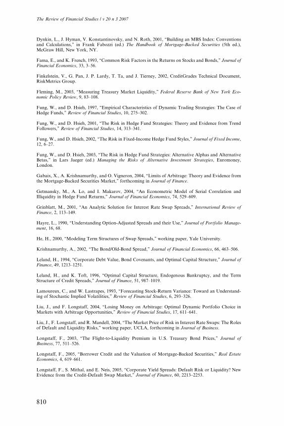
Dynkin, L., J. Hyman, V. Konstantinovsky, and N. Roth, 2001, ‘‘Building an MBS Index: Conventionsand Calculations,’’ in Frank Fabozzi (ed.) The Handbook of Mortgage-Backed Securities (5th ed.),McGraw Hill, New York, NY.

Fama, E., and K. French, 1993, ‘‘Common Risk Factors in the Returns on Stocks and Bonds,’’ Journal ofFinancial Economics, 33, 3–56.

Finkelstein, V., G. Pan, J. P. Lardy, T. Ta, and J. Tierney, 2002, CreditGrades Technical Document,RiskMetrics Group.

Fleming, M., 2003, ‘‘Measuring Treasury Market Liquidity,’’ Federal Reserve Bank of New York Eco-nomic Policy Review, 9, 83–108.

Fung, W., and D. Hsieh, 1997, ‘‘Empirical Characteristics of Dynamic Trading Strategies: The Case ofHedge Funds,’’ Review of Financial Studies, 10, 275–302.

Fung, W., and D. Hsieh, 2001, ‘‘The Risk in Hedge Fund Strategies: Theory and Evidence from TrendFollowers,’’ Review of Financial Studies, 14, 313–341.

Fung, W., and D. Hsieh, 2002, ‘‘The Risk in Fixed-Income Hedge Fund Styles,’’ Journal of Fixed Income,12, 6–27.

Fung, W., and D. Hsieh, 2003, ‘‘The Risk in Hedge Fund Strategies: Alternative Alphas and AlternativeBetas,’’ in Lars Jaeger (ed.) Managing the Risks of Alternative Investment Strategies, Euromoney,London.

Gabaix, X., A. Krishnamurthy, and O. Vigneron, 2004, ‘‘Limits of Arbitrage: Theory and Evidence fromthe Mortgage-Backed Securities Market,’’ forthcoming in Journal of Finance.

Getmansky, M., A. Lo, and I. Makarov, 2004, ‘‘An Econometric Model of Serial Correlation andIlliquidity in Hedge Fund Returns,’’ Journal of Financial Economics, 74, 529–609.

Grinblatt, M., 2001, ‘‘An Analytic Solution for Interest Rate Swap Spreads,’’ International Review ofFinance, 2, 113–149.

Hayre, L., 1990, ‘‘Understanding Option-Adjusted Spreads and their Use,’’ Journal of Portfolio Manage-ment, 16, 68.

He, H., 2000, ‘‘Modeling Term Structures of Swap Spreads,’’ working paper, Yale University.

Krishnamurthy, A., 2002, ‘‘The Bond/Old-Bond Spread,’’ Journal of Financial Economics, 66, 463–506.

Leland, H., 1994, ‘‘Corporate Debt Value, Bond Covenants, and Optimal Capital Structure,’’ Journal ofFinance, 49, 1213–1251.

Leland, H., and K. Toft, 1996, ‘‘Optimal Capital Structure, Endogenous Bankruptcy, and the TermStructure of Credit Spreads,’’ Journal of Finance, 51, 987–1019.

Lamoureux, C., and W. Lastrapes, 1993, ‘‘Forecasting Stock-Return Variance: Toward an Understand-ing of Stochastic Implied Volatilities,’’ Review of Financial Studies, 6, 293–326.

Liu, J., and F. Longstaff, 2004, ‘‘Losing Money on Arbitrage: Optimal Dynamic Portfolio Choice inMarkets with Arbitrage Opportunities,’’ Review of Financial Studies, 17, 611–641.

Liu, J., F. Longstaff, and R. Mandell, 2004, ‘‘The Market Price of Risk in Interest Rate Swaps: The Rolesof Default and Liquidity Risks,’’ working paper, UCLA, forthcoming in Journal of Business.

Longstaff, F., 2003, ‘‘The Flight-to-Liquidity Premium in U.S. Treasury Bond Prices,’’ Journal ofBusiness, 77, 511–526.

Longstaff, F., 2005, ‘‘Borrower Credit and the Valuation of Mortgage-Backed Securities,’’ Real EstateEconomics, 4, 619–661.

Longstaff, F., S. Mithal, and E. Neis, 2005, ‘‘Corporate Yield Spreads: Default Risk or Liquidity? NewEvidence from the Credit-Default Swap Market,’’ Journal of Finance, 60, 2213–2253.


810

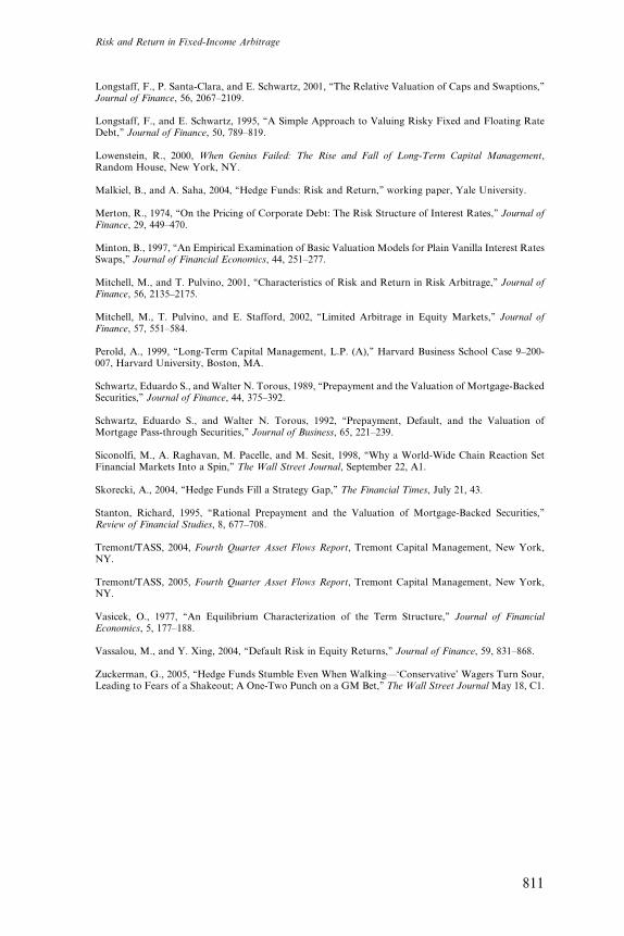
Longstaff, F., P. Santa-Clara, and E. Schwartz, 2001, ‘‘The Relative Valuation of Caps and Swaptions,’’Journal of Finance, 56, 2067–2109.

Longstaff, F., and E. Schwartz, 1995, ‘‘A Simple Approach to Valuing Risky Fixed and Floating RateDebt,’’ Journal of Finance, 50, 789–819.

Lowenstein, R., 2000, When Genius Failed: The Rise and Fall of Long-Term Capital Management,Random House, New York, NY.

Malkiel, B., and A. Saha, 2004, ‘‘Hedge Funds: Risk and Return,’’ working paper, Yale University.

Merton, R., 1974, ‘‘On the Pricing of Corporate Debt: The Risk Structure of Interest Rates,’’ Journal ofFinance, 29, 449–470.

Minton, B., 1997, ‘‘An Empirical Examination of Basic Valuation Models for Plain Vanilla Interest RatesSwaps,’’ Journal of Financial Economics, 44, 251–277.

Mitchell, M., and T. Pulvino, 2001, ‘‘Characteristics of Risk and Return in Risk Arbitrage,’’ Journal ofFinance, 56, 2135–2175.

Mitchell, M., T. Pulvino, and E. Stafford, 2002, ‘‘Limited Arbitrage in Equity Markets,’’ Journal ofFinance, 57, 551–584.

Perold, A., 1999, ‘‘Long-Term Capital Management, L.P. (A),’’ Harvard Business School Case 9–200-007, Harvard University, Boston, MA.

Schwartz, Eduardo S., and Walter N. Torous, 1989, ‘‘Prepayment and the Valuation of Mortgage-BackedSecurities,’’ Journal of Finance, 44, 375–392.

Schwartz, Eduardo S., and Walter N. Torous, 1992, ‘‘Prepayment, Default, and the Valuation ofMortgage Pass-through Securities,’’ Journal of Business, 65, 221–239.

Siconolfi, M., A. Raghavan, M. Pacelle, and M. Sesit, 1998, ‘‘Why a World-Wide Chain Reaction SetFinancial Markets Into a Spin,’’ The Wall Street Journal, September 22, A1.

Skorecki, A., 2004, ‘‘Hedge Funds Fill a Strategy Gap,’’ The Financial Times, July 21, 43.

Stanton, Richard, 1995, ‘‘Rational Prepayment and the Valuation of Mortgage-Backed Securities,’’Review of Financial Studies, 8, 677–708.

Tremont/TASS, 2004, Fourth Quarter Asset Flows Report, Tremont Capital Management, New York,NY.

Tremont/TASS, 2005, Fourth Quarter Asset Flows Report, Tremont Capital Management, New York,NY.

Vasicek, O., 1977, ‘‘An Equilibrium Characterization of the Term Structure,’’ Journal of FinancialEconomics, 5, 177–188.

Vassalou, M., and Y. Xing, 2004, ‘‘Default Risk in Equity Returns,’’ Journal of Finance, 59, 831–868.

Zuckerman, G., 2005, ‘‘Hedge Funds Stumble Even When Walking—‘Conservative’ Wagers Turn Sour,Leading to Fears of a Shakeout; A One-Two Punch on a GM Bet,’’ The Wall Street Journal May 18, C1.


811

Documents

Risk and Return in Fixed-Income Arbitrage: Nickels in ...jd10/nickelsRFS.pdf · Risk and Return in Fixed-Income Arbitrage: Nickels in Front of a Steamroller? Jefferson Duarte University