Rise of the Machines: Algorithmic Trading in the Foreign

Exchange Market

Alain Chaboud Benjamin Chiquoine Erik Hjalmarsson Clara Vega�

February 20, 2013

Abstract

We study the impact of algorithmic trading in the foreign exchange market using a long time series of

high-frequency data that speci�cally identi�es computer-generated trading activity. Using both a reduced-

form and a structural estimation, we �nd clear evidence that algorithmic trading causes an improvement

in two measures of price e¢ ciency in this market: the frequency of triangular arbitrage opportunities and

the autocorrelation of high-frequency returns. Relating our results to the recent theoretical literature on

the subject, we show that the reduction in arbitrage opportunities is associated primarily with comput-

ers taking liquidity, while the reduction in the autocorrelation of returns owes more to the algorithmic

provision of liquidity. We also �nd evidence that algorithmic trades and strategies are more correlated

than those of non-algorithmic traders. However, the analysis shows that this high degree of correlation

does not appear to cause a degradation in market quality.

�JEL Classi�cation: F3, G12, G14, G15. Keywords: Algorithmic trading; Price discovery. Chaboud and Vega are with theDivision of International Finance, Federal Reserve Board, Mail Stop 43, Washington, DC 20551, USA; Chiquoine is with theStanford Management Company, 635 Knight Way, Stanford CA 94305, USA; Hjalmarsson is with Queen Mary, University ofLondon, School of Economics and Finance, Mile End Road, London E1 4NS, UK. Please address comments to the authors viae-mail at alain.p.chaboud@frb.gov, bchiquoine@ti¤.org, e.hjalmarsson@qmul.ac.uk, and clara.vega@frb.gov. We are grateful toEBS/ICAP for providing the data, and to Nicholas Klagge and James S. Hebden for their excellent research assistance. Wewould like to thank Cam Harvey, an anonymous Associate Editor, an anonymous Advisory Editor, and an anonymous referee fortheir valuable comments. We also bene�ted from the comments of Gordon Bodnar, Charles Jones, Terrence Hendershott, LuisMarques, Albert Menkveld, Dag�nn Rime, Alec Schmidt, John Schoen, Noah Sto¤man, and of participants in the University ofWashington Finance Seminar, SEC Finance Seminar Series, Spring 2009 Market Microstructure NBER conference, San FranciscoAEA 2009 meetings, the SAIS International Economics Seminar, the SITE 2009 conference at Stanford, the Barcelona EEA2009 meetings, the Essex Business School Finance Seminar, the EDHEC Business School Finance Seminar, and the ImperialCollege Business School Finance Seminar. The views in this paper are solely the responsibility of the authors and should not beinterpreted as re�ecting the views of the Board of Governors of the Federal Reserve System or of any other person associatedwith the Federal Reserve System.

1 Introduction

The use of algorithmic trading (AT), where computers monitor markets and manage the trading process at

high frequency, has become common in major �nancial markets in recent years, beginning in the U.S. equity

market in the 1990s. Since the introduction of algorithmic trading, there has been widespread interest in

understanding the potential impact it may have on market dynamics, particularly recently following several

trading disturbances in the equity market blamed on computer-driven trading. While some have highlighted

the potential for more e¢ cient price discovery, others have expressed concern that it may lead to higher

adverse selection costs and excess volatility.1 In this paper we analyze the e¤ect algorithmic (�computer�)

trades and non-algorithmic (�human�) trades have on the informational e¢ ciency of foreign exchange prices;

it is the �rst formal empirical study on the subject in the foreign exchange market.

We rely on a novel data set consisting of several years (September 2003 to December 2007) of minute-

by-minute trading data from Electronic Broking Services (EBS) in three currency pairs: the euro-dollar,

dollar-yen, and euro-yen. The data represent a large share of spot interdealer transactions across the globe in

these exchange rates, with EBS widely considered to be the primary site of price discovery in these currency

pairs during our sample period. A crucial feature of the data is that, on a minute-by-minute frequency, the

volume and direction of human and computer trades are explicitly identi�ed, allowing us to measure their

respective impacts at high frequency. Another useful feature of the data is that it spans the introduction and

rapid growth of algorithmic trading in an important market where it had not been previously allowed.

The theoretical literature highlights two main di¤erences between computer and human traders. First,

computers are faster than humans, both in processing information and in acting on that information. Sec-

ond, there is the potential for higher correlation in computers�trading actions than in those of humans, as

computers need to be pre-programmed and may react similarly to a given signal. There is no agreement,

however, on the impact that these features of algorithmic trading may have on the price discovery process.

Biais, Foucault, and Moinas (2011) and Martinez and Rosu (2011) argue that the speed advantage of

algorithmic traders over humans � speci�cally their ability to react more quickly to public information �

should have a positive e¤ect on the informativeness of prices. In their theoretical models, algorithmic traders

are better informed than humans and use market orders to exploit their information. Given these assumptions,

the authors show that the presence of algorithmic traders makes asset prices more informationally e¢ cient,

but that their trades are a source of adverse selection for those who provide liquidity. They argue that

algorithmic traders contribute to price discovery because, once price ine¢ ciencies arise, AT quickly makes

them disappear by trading on posted quotes. Similarly Oehmke (2009) and Kondor (2009), in the context

1Biais and Woolley (2011) and Foucault (2012) provide excellent surveys of the recent literature on this topic.

1

of traders who implement �convergence trade�strategies (i.e., strategies taking long-short positions in assets

with identical underlying cash �ows that temporarily trade at di¤erent prices), argue that the higher the

number of traders who implement those strategies, the more e¢ cient prices will be. One could also advance,

as does Ho¤mann (2012), that better informed algorithmic traders who specialize in providing liquidity make

prices more informationally e¢ cient by posting quotes that re�ect new information quickly, thus preventing

arbitrage opportunities from occurring in the �rst place.

In contrast to these positive views on algorithmic trading and price e¢ ciency, Foucault, Hombert, and

Rosu (2012) point out that, in a world with no asymmetric information, the speed advantage of algorithmic

traders would not increase the informativeness of prices but would still increase adverse selection costs. Jarrow

and Protter (2011) argue that both features of AT, the speed advantage over human traders and the potential

commonality of trading actions amongst computers, may have a negative e¤ect on the informativeness of

prices. In their theoretical model, algorithmic traders, triggered by a common signal, initiate the same

trade at the same time. Algorithmic traders collectively act as one �big trader�, create price momentum

and thus cause prices to be less informationally e¢ cient.2 Kozhan and Wah Tham (2012), in contrast to

Oehmke�s (2009) and Kondor�s (2009) more standard notion that competition improves price e¢ ciency, argue

that computers entering the same trade at the same time to exploit an arbitrage opportunity could cause

a crowding e¤ect, which in turn would push prices away from their fundamental values. Stein (2009) also

highlights this crowding e¤ect in the context of hedge funds simultaneously implementing �convergence trade�

strategies.

Guided by these theoretical papers, our paper studies the impact of algorithmic trading on the price

discovery process in the foreign exchange market. Besides giving us a measure of the relative participation

of computers and humans in trades, our data also allows us to study more precisely how algorithmic trading

a¤ects price discovery. We study separately, in particular, the impact of trades where computers are providing

liquidity to the market and trades where computers are taking liquidity from the market, addressing one of

the questions posed in the literature. We also look at how the share of the market�s order �ow generated by

algorithmic traders impacts price discovery. Finally, to address another concern highlighted in the literature�

namely that the trading strategies used by computers are more correlated than those used by humans,

potentially creating excessive volatility� we propose a novel way of indirectly inferring the correlation among

computer trading strategies from our trading data. The primary idea behind the measure that we design is

that traders who follow similar trading strategies will trade less with each other than those who follow less

correlated strategies.

2One could also argue that if algorithmic traders behave, as a group, like the positive-feedback traders of DeLong, Shleifer,Summers, and Waldman (1990) or the chartists described in Froot, Scharfstein, and Stein (1992), or the short-term investors inVives (1995), then their activity, in total, would likely increase excess volatility.

2

We �rst use our data to study the impact of algorithmic trading on the frequency of triangular arbitrage

opportunities amongst the euro-dollar, dollar-yen, and euro-yen currency pairs. These arbitrage opportunities

are a clear example of prices not being informationally e¢ cient in the foreign exchange market. We document

that the introduction and growth of algorithmic trading coincided with a substantial reduction in triangular

arbitrage opportunities. We then continue with a formal analysis of whether algorithmic trading activity

causes a reduction in triangular arbitrage opportunities, or whether the relationship is merely coincidental,

possibly due to a concurrent increase in trading volume or decrease in price volatility. To that end, we

formulate a high-frequency vector autoregression (VAR) speci�cation that models the interaction between

triangular arbitrage opportunities and algorithmic trading (the overall share of algorithmic trading and the

various facets of algorithmic activity discussed above). In the VAR speci�cation, we control for time trends,

trading volume, and exchange rate return volatility in each currency pair. We estimate both a reduced form

of the VAR and a structural VAR which uses the heteroskedasticity identi�cation approach developed by

Rigobon (2003) and Rigobon and Sack (2003, 2004).3 In contrast to the reduced-form Granger causality tests,

which essentially measure predictive relationships, the structural VAR estimation allows for an identi�cation

of the contemporaneous causal impact of algorithmic trading on triangular arbitrage opportunities.

Both the reduced-form and structural-form VAR estimations show that algorithmic trading activity causes

a reduction in the number of triangular arbitrage opportunities. In addition, we �nd that algorithmic traders

reduce arbitrage opportunities more by acting on the quotes posted by non-algorithmic traders than by

posting quotes that are then traded upon. This result is consistent with the view that algorithmic trading

improves informational e¢ ciency by speeding up price discovery, but that, at the same time, it increases the

adverse selection costs to slower traders, as suggested by the theoretical models of Biais, Foucault, and Moinas

(2011) and Martinez and Rosu (2011). We also �nd that a higher degree of correlation amongst algorithmic

trading strategies reduces the number of arbitrage opportunities over our sample period. Thus, contrary to

Jarrow and Protter (2011) and Kozhan and Wah Tham (2012), in this particular example commonality in

trading strategies appears to be bene�cial to the e¢ ciency of the price discovery process.

The impact of algorithmic trading on the frequency of triangular arbitrage opportunities is, however, only

one facet of how computers may a¤ect the price discovery process. More generally, we investigate whether

algorithmic trading contributes to the temporary deviation of asset prices from their fundamental values,

resulting in excess volatility, particularly at high frequencies, as suggested by Jarrow and Protter (2011) and

Kozhan and Wah Tham (2012). To investigate the e¤ect of algorithmic trading on this aspect of informational

e¢ ciency, we study the autocorrelation of high-frequency returns in our three exchange rates.4 We again

3To identify the parameters of the structural VAR, we use the heteroskedasticity in algorithmic trading activity across thesample.

4We use the term �excess volatility� to refer to any variation in prices that is not solely re�ecting changes in the underlying

3

estimate both a reduced form and a structural VAR and �nd that, on average, an increase in algorithmic

trading participation in the market causes a reduction in the degree of autocorrelation of high-frequency

returns. Interestingly, we �nd that the improvement in the informational e¢ ciency of prices now seems to

come predominantly from an increase in the trading activity of algorithmic traders when they are providing

liquidity� that is, posting quotes which are hit� not from an increase in the trading activity of algorithmic

traders who hit posted quotes. In other words, in this case, in contrast to the study of triangular arbitrage,

algorithmic traders appear to increase the informational e¢ ciency of prices by posting quotes that re�ect

new information more quickly, consistent with Ho¤mann (2012).

Also in contrast to the triangular arbitrage case, we do not �nd a statistically signi�cant association

between a higher correlation of algorithmic traders�actions and high-frequency return autocorrelation. The

di¤erence between the autocorrelation results and those for triangular arbitrage may o¤er some support

for one of the conclusions of Foucault (2012): The e¤ect of algorithmic trading on the informativeness of

prices may ultimately depend on the type of strategies used by algorithmic traders, not on the presence of

algorithmic trading per se.

The paper proceeds as follows. In Section 2, we brie�y discuss the related empirical literature on the e¤ect

of algorithmic trading on market quality. Section 3 introduces the high-frequency data used in this study,

including a short description of the structure of the market and an overview of the growth of algorithmic

trading in the foreign exchange market over time. In Section 4, we present our measures of the various

aspects of algorithmic trading, including whether actions by computer traders are more correlated than those

of human traders. In Sections 5 and 6, we test whether there is evidence that algorithmic trading activity

has a causal impact on the informativeness of prices, looking �rst at triangular arbitrage and then at high-

frequency return autocorrelation. Finally, Section 7 concludes. Some additional clarifying and technical

material is found in the Appendix.

2 Related Empirical Literature

Our study contributes to the new empirical literature on the impact of algorithmic trading on various measures

of market quality, with the vast majority of the studies focusing on equity markets. A number of these studies

use proxies to measure the share of algorithmic trading in the market. Hendershott, Jones, and Menkveld

(2011), in one of the earliest studies, use, for instance, the �ow of electronic messages on the NYSE after

the implementation of Autoquote as a proxy for algorithmic trading. They �nd that algorithmic trading

e¢ cient price process. Under the usual assumption that e¢ cient prices follow a random walk speci�cation (see discussionin Footnote 20), autocorrelation in returns therefore imply some form of excess volatility and temporary deviations from thee¢ cient price. When discussing the empirical results, we use the terms autocorrelation and excess volatility interchangeably.

4

improves standard measures of liquidity (the quoted and e¤ective bid-ask spreads). They attribute the decline

in spreads to a decline in adverse selection � a decrease in the amount of price discovery associated with

trading activity and an increase in the amount of price discovery that occurs without trading. The authors�

interpretation of the empirical evidence is that computers enhance the informativeness of quotes by more

quickly resetting their quotes after news arrivals. Boehmer, Fong, and Wu (2012) use a similar identi�cation

strategy to that of Hendershott, Jones, and Menkveld (2011). Rather than using the implementation of

Autoquote, however, they use the �rst availability of co-location facilities around the world to identify the

e¤ect algorithmic trading activity has on liquidity, short-term volatility, and the informational e¢ ciency of

stock prices. Hendershott and Riordan (2012) use one month of algorithmic trading data in the 30 DAX

stocks traded on the Deutsche Boerse and �nd that algorithmic traders improve market liquidity by providing

liquidity when it is scarce, and consuming it when it is plentiful.

Some recent studies have focused more speci�cally on the impact of high-frequency trading (HFT), gener-

ally viewed as a subset of algorithmic trading (not all algorithmic traders trade at extremely high frequency).

For instance Brogaard, Hendershott, and Riordan (2012) use NASDAQ data from 2008 and 2009 and �nd

that high-frequency traders (HFTs) facilitate price e¢ ciency by trading in the direction of permanent price

changes during macroeconomic news announcement times and at other times. Hirschey (2011), using a similar

database to that of Brogaard, Hendershott, and Riordan (2012), �nds that HFT�s aggressive purchases (sales)

predict future aggressive purchases (sales) by non-HFTs. Both of these studies suggest that HFTs are the

�informed�traders. Hasbrouck and Saar (2012) develop an algorithm to proxy for overall HFT activity and

conclude that HFT activity reduces short-term volatility and bid-ask spreads, and that it increases displayed

depth in the limit order book. Menkveld (2011) analyzes the trading strategy of one large HFT in the Chi-X

market and concludes that the HFT behaves like a fast version of the classic market maker. Kirilenko, Kyle,

Samadi, and Tuzun (2011) study the role HFTs played during the May 6, 2010 ��ash crash�and conclude

that HFTs did not trigger the crash, but that they contributed to the crash by pulling out of the market as

market conditions became challenging.

Our work complements these studies in several dimensions. First, of, course, we study, for the �rst

time, a di¤erent asset class, foreign exchange, which is traded in a very large global market.5 We have a

long data set which clearly identi�es computer-generated trades without appealing to proxies, and which

5The structure of the wholesale spot foreign exchange market is obviously di¤erent from that of the major equity markets,but some of the di¤erences probably facilitate the analysis of the impact of AT. In particular, while there are several platformswhere one can trade foreign exchange in large quantities, price discovery in the currency pairs we study occurs overwhelminglyon one platform, EBS, the source of our data. In addition, unlike a number of equity trading venues, traders do not get rebatesfor providing liquidity on EBS, which may allow for a �cleaner� study of the role of AT making and taking in price discovery.Finally, in the foreign exchange market, AT potentially causes a smaller increase in adverse selection costs than it may cause inthe equity market because it is a wholesale market. The minimum trade size is one million of the base currency, and thus thereare no �small�market participants.

5

spans the introduction of algorithmic trading in the market. The data also permits us to di¤erentiate the

e¤ects of certain features of algorithmic trading, separating, for instance, trades initiated by a computer

and trades initiated by a human, which in turn allows us to address recently-developed theories on how

algorithmic trading impacts price discovery. We have data on three interrelated exchange rates, and therefore

can analyze the impact of computer trades on the frequency of a very obvious type of arbitrage opportunity.

And, �nally, we study the correlation of algorithmic trading strategies and its impact on the informational

e¢ ciency of prices, also relating our �ndings to the recent theoretical literature.

3 Data Description

3.1 Market Structure

Over our sample period, from 2003 to 2007, two electronic platforms process a majority of global interdealer

spot trading in the major currency pairs, one o¤ered by Reuters, and one o¤ered by Electronic Broking

Services (EBS). Both of these trading platforms are electronic limit order books. Importantly, trading in

each major currency pair is highly concentrated on only one of the two systems. Of the most traded currency

pairs (exchange rates), the top two, euro-dollar and dollar-yen, trade primarily on EBS, while the third,

sterling-dollar, trades primarily on Reuters. As a result, price discovery for spot euro-dollar, for instance,

occurs on the EBS system, and dealers across the globe base their spot and derivative quotes on that price.

EBS controls the network and each of the terminals on which the trading is conducted. Traders can enter

trading instructions manually, using an EBS keyboard, or, upon approval, via a computer directly interfacing

with the system. The type of trader (human or computer) behind each trading instruction is recorded by

EBS, allowing for our study.

The EBS system is an interdealer system accessible to foreign exchange dealing banks and, under the

auspices of dealing banks (via prime brokerage arrangements), to hedge funds and commodity trading advisors

(CTAs). As it is a �wholesale�trading system, the minimum trade size over our sample period is 1 million of

the �base�currency, and trade sizes are only allowed in multiple of millions of the base currency. We analyze

data in the three most-traded currency pairs on EBS, euro-dollar, dollar-yen, and euro-yen.6

3.2 Quote and Transaction Data

Our data consists of both quote data and transactions data. The quote data, at the one-second frequency,

consist of the highest bid quote and the lowest ask quote on the EBS system in our three currency pairs. The

6The euro-dollar currency pair is quoted as an exchange rate in dollars per euro, with the euro the �base�currency. Similarly,the euro is also the base currency for euro-yen, while the dollar is the base currency for the dollar-yen pair.

6

quote data are available from 1997 through 2007. All the quotes are executable and therefore truly represent

the market price at that instant. From these data, we construct mid-quote series from which we compute

exchange rate returns at various frequencies. The transactions data, available from October 2003 through

December 2007, are aggregated by EBS at the one-minute frequency. Throughout the subsequent analysis,

we focus on data sampled between 3am and 11am New York time, which represent the most active trading

hours of the day (see Berger et al., 2008, for further discussion on trading activity on the EBS system). That

is, each day in our sample is made up of the intra-daily observation between 3am and 11am New York time.7

The transaction data provide detailed information on the volume and direction of trades that can be

attributed to computers and humans in each currency pair. Speci�cally, each minute we observe trading

volume and order �ow for each of the four possible pairs of human and computer makers and takers: human-

maker/human-taker (HH), computer-maker/human-taker (CH), human-maker/computer-taker (HC), and

computer-maker/computer-taker (CC).8 Order �ow is de�ned, as is common, as the net of buyer-initiated

trading volume minus seller-initiated trading volume, with traders buying or selling the base currency. We

denote the trading volume and order �ow attributable to any maker-taker pair as V ol (�) and OF (�), respec-

tively.

Figure 1 shows, from 2003 through 2007, for each currency pair, the percent of trading volume where

at least one of the two counterparties is an algorithmic trader. We label this variable, V AT = 100 �V ol(CH+HC+CC)

V ol(HH+CH+HC+CC) . From its beginning in late 2003, the fraction of trading volume involving algorithmic

trading for at least one of the counterparts grows by the end of 2007 to near 60 percent for euro-dollar and

dollar-yen trading, and to about 80 percent for euro-yen trading.

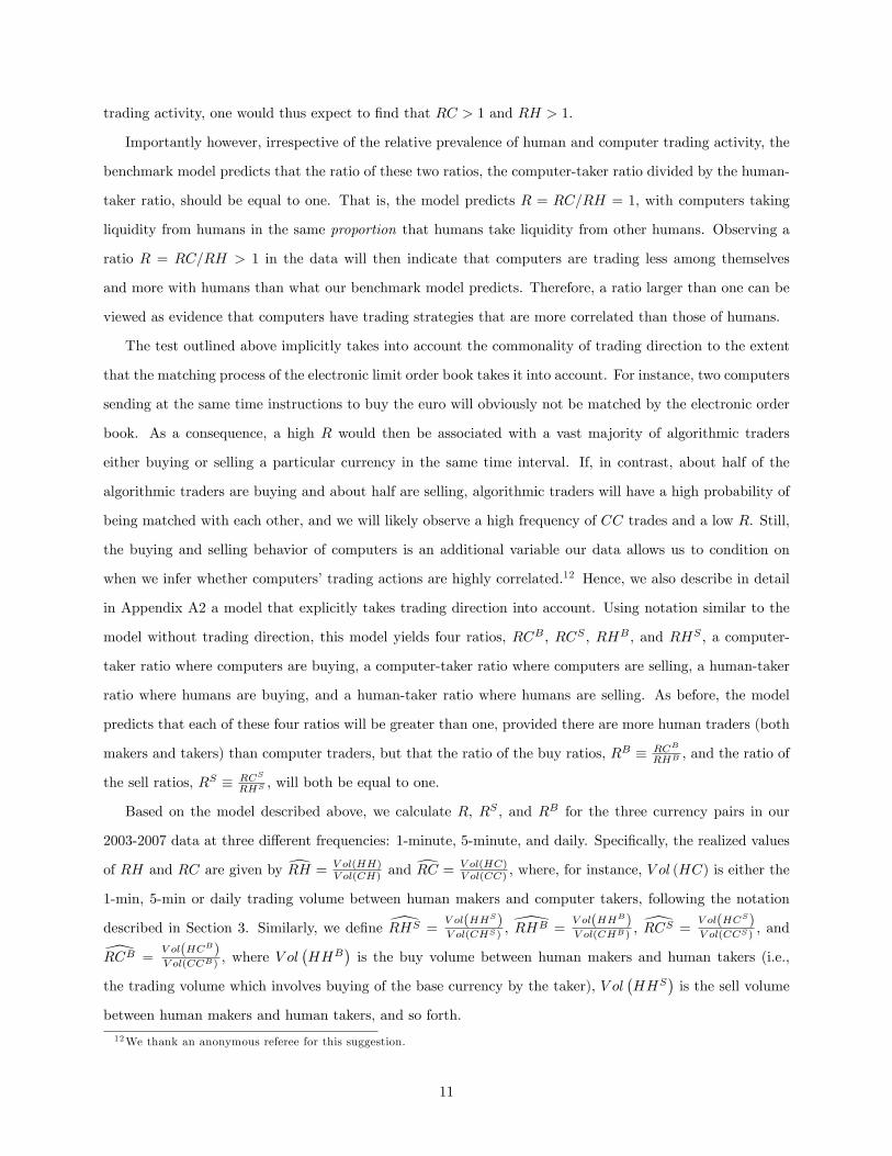
Figure 2 shows the evolution over time of the four di¤erent possible types of trades: V ol(HH), V ol(CH),

V ol(HC), and V ol(CC); as fractions of the total volume. By the end of 2007, in the euro-dollar and dollar-

yen markets, human to human trades, the solid lines, account for slightly less than half of the volume, and

computer to computer trades, the dotted lines, for about ten to �fteen percent. In these two currency pairs,

V ol(CH) is often close to V ol(HC), i.e., computers take prices posted by humans, the dashed lines, about

as often as humans take prices posted by market-making computers, the dotted-dashed lines. The story is

di¤erent for the cross-rate, the euro-yen currency pair. By the end of 2007, there are more computer to

computer trades than human to human trades. But the most common type of trade in euro-yen is computers7We exclude data collected from Friday 17:00 through Sunday 17:00 New York time from our sample, as activity on the system

during these �non-standard� hours is minimal and not encouraged by the foreign exchange community. Trading is continuousoutside of the weekend, but the value date for trades, by convention, changes at 17:00 New York time, which therefore marksthe end of each (full) trading day. We also drop certain holidays and days of unusually light volume: December 24-December26, December 31-January 2, Good Friday, Easter Monday, Memorial Day, Labor Day, Thanksgiving and the following day, andJuly 4 (or, if this is on a weekend, the day on which the U.S. Independence Day holiday is observed).

8The naming convention for �maker�and �taker� re�ects the fact that the �maker�posts quotes before the �taker� choosesto trade at that price. Posting quotes is, of course, the traditional role of the market-�maker.� The taker is also often viewedas the �aggressor� or the �initiator� of the trade. We refer the reader to Appendix A1 for more details on how we calculatevolume and order �ow for these four possible pairs of human and computer makers and takers.

7

trading on prices posted by humans. We believe this re�ects computers taking advantage of short-lived

triangular arbitrage opportunities, where prices set in the euro-dollar and dollar-yen markets, the primary

sites of price discovery, are very brie�y out of line with the euro-yen cross rate. Detecting and trading on

triangular arbitrage opportunities is widely thought to have been one of the �rst strategies implemented

by algorithmic traders in the foreign exchange market, which is consistent with the more rapid growth in

algorithmic activity in the euro-yen market documented in Figure 1. We discuss the evolution of the frequency

of triangular arbitrage opportunities in Section 5 of the paper.

4 Measuring Various Features of Algorithmic Trading

4.1 An Illustrative Example

Before describing the variables we use to test the impact of various features of algorithmic trading, we �rst

show an interesting illustrative example. Jarrow and Protter (2011) argue that the potential commonality of

trading strategies amongst algorithmic traders may have a negative e¤ect on the informativeness of prices.

In their theoretical model, algorithmic traders, triggered by a common signal, do the same trade at the same

time. Algorithmic traders collectively act as one big trader, create price momentum and thus cause prices to

be less informationally e¢ cient. Similarly, Khandani and Lo (2007, 2011), who analyze the large losses that

occurred for many quantitative long-short equity strategies at the beginning of August 2007, highlight the

possible adverse e¤ects on the market of such commonality in behavior across market participants (algorithmic

or not, in their analysis) and provide empirical support for this concern.

If one looks for similar episodes in our data, August 16, 2007 in the dollar-yen market stands out. It is

the day with the highest realized volatility and with one of the highest absolute values of autocorrelation

in 5-second returns in our sample period. On that day, the Japanese yen appreciated sharply against the

U.S. dollar around 6:00 a.m. and 12:00 p.m. (NY time), as shown in Figure 3. The �gure also shows,

for each 30-minute interval in the day, computer order �ow (HC + CC) in the top panel and human order

�ow (HH + CH) in the lower panel. The two sharp exchange rate movements mentioned happened when

computers, as a group, aggressively initiated sales of dollars and purchases of yen. Computers, during these

periods of sharp yen appreciation, mainly traded with humans, not with other computers. Human order

�ow at those times was, in contrast, quite small, even though the trading volume initiated by humans (not

shown) was well above that initiated by computers: human takers were therefore selling and buying dollars

in almost equal amounts. The orders initiated by computers during those time intervals were therefore far

more correlated than the orders initiated by humans. After 12:00 p.m., human traders, in aggregate, began

8

to buy dollars fairly aggressively, and the appreciation of the yen against the dollar was partially reversed.

The August 16, 2007 episode in the dollar-yen market was widely viewed at the time as the result of a

sudden unwinding of large yen carry-trade positions, with many hedge funds and banks�proprietary trading

desks closing risky positions and buying yen to pay back low-interest loans.9 This is, of course, only one

episode in our �ve-year sample, and by far the most extreme as to its impact on volatility, so one should not

draw conclusions about the overall correlation of algorithmic strategies or the impact of algorithmic order

�ow based on this single instance. Furthermore, episodes of very sharp appreciation of the yen due to the

rapid unwinding of yen carry trades have occurred on several occasions since the late 1990s, well before

algorithmic trading was allowed in this market.10 Still, this example is a good illustration of the type of

market event that has been linked, fairly or unfairly, to the rise of algorithmic trading. It is also a simple

example of how our data can be used to analyze such events.

4.2 Inferring The Correlation of Algorithmic Strategies from Trade Data: The

R-Measure

There is little solid information, and certainly no data, about the mix of strategies used by algorithmic traders

in the foreign exchange market, as traders and EBS keep what they know con�dential. From conversations

with market participants, however, we believe that, over our sample period, about half of the algorithmic

trading volume on EBS comes from traditional foreign exchange dealing banks, with the other half coming

from hedge funds and commodity trading advisors (CTAs). Hedge funds and CTAs, who access EBS under

prime-brokerage arrangements, can only trade algorithmically over our sample period. Some of the banks�

computer trading in our sample is related to activity on their own customer-to-dealer platforms, to automated

hedging activity, and to the optimal execution of large orders. But a sizable fraction (perhaps almost a half) is

believed to be proprietary trading using a mix of strategies similar to what hedge funds and CTAs use. These

strategies include various types of high-frequency arbitrage, including some across di¤erent asset markets,

a number of lower-frequency statistical arbitrage strategies (including carry trades), and strategies designed

to automatically react to news and data releases (still fairly rare in the foreign exchange market by 2007).

Overall, market participants believe that the main di¤erence between the mix of algorithmic strategies used

in the foreign exchange market and the mix used in the equity market is that optimal execution algorithms

9A traditional carry-trade strategy borrows in a low-interest rate currency and invests in a high-interest rate currency, withthe implicit assumption that the interest rate di¤erential will not be (fully) o¤set by changes in the exchange rate. That is,carry trades bet on uncovered interest rate parity not holding. The August 16, 2007 episode occurs only a week after the eventsdescribed in Khandani and Lo (2007, 2011), a time of high stress for many quantitative long/short equty hedge funds. We arenot aware of any proven link between the quant equity crisis and the carry trade unwinding, but the precarious �nancial positionof several hedge funds at that time may have contributed to the sharp movements in the dollar-yen exchange rate.10The sharp move of the yen in October 1998, which included a 1-day appreciation of the yen against the dollar of more than

7 percent, is the best-known example of the impact of the rapid unwinding of carry trades.

9

are less prevalent in foreign exchange than in equity.

As mentioned previously, a concern expressed by the literature about algorithmic traders is that their

strategies, which have to be pre-programmed, may be less diverse, more correlated, than those of humans.11

Computers could then react in the same fashion, at the same time, to the same information, creating excess

volatility in the market, particularly at high frequency, as suggested by our August 16, 2007 carry-trade

example above. While we do not observe the trading strategies of our market participants, we can derive

some information about the correlation of algorithmic strategies from the trading activity of computers and

humans. The intuitive idea is the following. Traders who follow similar trading strategies and therefore

send similar trading instructions at the same time, will trade less with each other than those who follow

less correlated strategies. Therefore, the extent to which computers trade (or do not trade) with each other

should contain information about how correlated their algorithmic strategies are.

More precisely, to extract this information, we �rst consider a simple benchmark model that assumes

random and independent matching of traders. This is a reasonable assumption given the lack of discrimination

between keyboard traders and algorithmic traders in the EBS matching process; that is, EBS does not

di¤erentiate in any way between humans and computers when matching buy and sell orders in its electronic

order book. Traders also do not know the identity and type of trader they have been matched with until after

the full trade is complete. The model allows us to determine the theoretical probabilities of the four possible

types of trades: Human-maker/human-taker, computer-maker/human-taker, human-maker/computer-taker

and computer-maker/computer-taker. We then compare these theoretical probabilities to those observed in

the actual trading data. The benchmark model is fully described in Appendix A2, and below we outline the

main concepts and empirical results.

Under our random and independent matching assumption, computers and humans, both of which are in-

di¤erent ex-ante between making and taking, trade with each other in proportion to their relative presence in

the market. For instance, in a world with more human trading activity than computer trading activity (which

is the case in most of our sample), we should observe that computers take more liquidity from humans than

from other computers. That is, the probability of observing human-maker/computer-taker trades, Prob(HC),

should be larger than the probability of observing computer-maker/computer taker trades, Prob(CC). We

label the ratio of the two, Prob(HC)/Prob(CC), the computer-taker ratio, RC. Similarly, under our as-

sumption, in such a world one would expect humans to take more liquidity from other humans than from

computers, i.e., Prob(HH) should be larger than Prob(CH). We label this ratio, Prob(HH)/Prob(CH),

the human-taker ratio, RH. In summary, in our data with more human trading activity than computer

11As pointed out by the referee, it is true that algorithms are necessarily rule-based at very high execution frequencies, butat a somewhat lower frequency, human monitoring is still common for a variety of algorithms.

10

trading activity, one would thus expect to �nd that RC > 1 and RH > 1.

Importantly however, irrespective of the relative prevalence of human and computer trading activity, the

benchmark model predicts that the ratio of these two ratios, the computer-taker ratio divided by the human-

taker ratio, should be equal to one. That is, the model predicts R = RC=RH = 1, with computers taking

liquidity from humans in the same proportion that humans take liquidity from other humans. Observing a

ratio R = RC=RH > 1 in the data will then indicate that computers are trading less among themselves

and more with humans than what our benchmark model predicts. Therefore, a ratio larger than one can be

viewed as evidence that computers have trading strategies that are more correlated than those of humans.

The test outlined above implicitly takes into account the commonality of trading direction to the extent

that the matching process of the electronic limit order book takes it into account. For instance, two computers

sending at the same time instructions to buy the euro will obviously not be matched by the electronic order

book. As a consequence, a high R would then be associated with a vast majority of algorithmic traders

either buying or selling a particular currency in the same time interval. If, in contrast, about half of the

algorithmic traders are buying and about half are selling, algorithmic traders will have a high probability of

being matched with each other, and we will likely observe a high frequency of CC trades and a low R. Still,

the buying and selling behavior of computers is an additional variable our data allows us to condition on

when we infer whether computers�trading actions are highly correlated.12 Hence, we also describe in detail

in Appendix A2 a model that explicitly takes trading direction into account. Using notation similar to the

model without trading direction, this model yields four ratios, RCB , RCS , RHB , and RHS , a computer-

taker ratio where computers are buying, a computer-taker ratio where computers are selling, a human-taker

ratio where humans are buying, and a human-taker ratio where humans are selling. As before, the model

predicts that each of these four ratios will be greater than one, provided there are more human traders (both

makers and takers) than computer traders, but that the ratio of the buy ratios, RB � RCB

RHB , and the ratio of

the sell ratios, RS � RCS

RHS , will both be equal to one.

Based on the model described above, we calculate R, RS , and RB for the three currency pairs in our

2003-2007 data at three di¤erent frequencies: 1-minute, 5-minute, and daily. Speci�cally, the realized values

of RH and RC are given by dRH = V ol(HH)V ol(CH) and

dRC = V ol(HC)V ol(CC) , where, for instance, V ol (HC) is either the

1-min, 5-min or daily trading volume between human makers and computer takers, following the notation

described in Section 3. Similarly, we de�ne [RHS =V ol(HHS)V ol(CHS)

, \RHB =V ol(HHB)V ol(CHB)

, [RCS = V ol(HCS)V ol(CCS)

, and

[RCB =V ol(HCB)V ol(CCB)

, where V ol�HHB

�is the buy volume between human makers and human takers (i.e.,

the trading volume which involves buying of the base currency by the taker), V ol�HHS

�is the sell volume

between human makers and human takers, and so forth.

12We thank an anonymous referee for this suggestion.

11

Table 1 shows the means of the natural log of the 1-min, 5-min, and daily ratios of ratios, ln bR = ln(dRCdRH ),ln cRS = ln(

[RCS

[RHS), and lndRB = ln(

[RCB

\RHB), calculated for each currency pair in our data.13 In contrast to

the benchmark predictions that R � 1; RB � 1 and RS � 1, or equivalently that lnR � 0; lnRB � 0 and

lnRS � 0; we �nd that, for all three currency pairs, at all frequencies, ln bR , lndRB and ln cRS are substantiallyand signi�cantly greater than zero. The table also shows the number of periods in which the statistics are

above zero. In all currencies, at the daily frequency, ln bR , lndRB and ln cRS are above zero for more than 95percent of the days.14 Overall, the observed ratios are highest in the cross-rate, the euro-yen, consistent with

the view that a large fraction of computer traders in the cross-rate may be attempting to take advantage of

the same short-lived triangular arbitrage opportunities, and thus are more likely to send the same trading

instructions at the same time in this currency pair. In summary, the results show that computers do not

trade with each other as much as random matching would predict. We take this as evidence that the trading

strategies used by algorithmic traders are less diverse than the trading strategies used by human traders. The

R-Measure, a re�ection of the correlation of algorithmic strategies, is one of the variables we use to analyze

the impact of algorithmic trading on triangular arbitrage opportunities and on the absolute value of return

autocorrelation. We next describe the other variables we create to measure certain features of algorithmic

trading activity, variables which we will also use in our analysis.

4.3 Measuring Other Features of Algorithmic Trading Activity

With our trading data providing information, minute by minute, on the volume of trade, direction of trade,

and initiating of the trade attributed to algorithmic (computer) and non-algorithmic (human) traders, we can

study not just the overall impact of the presence of algorithmic trading in the market but also the mechanism

by which algorithmic trading a¤ects the market. To this e¤ect, we create several variables at a minute-by-

minute frequency to use in the analysis. (1) We measure overall algorithmic trading activity as the fraction

of total volume where a computer is at least one of the two counterparts of a trade. As explained before,

we label this variable V AT = 100 � V ol(HC)+V ol(CH)+V ol(CC)V ol(HH)+V ol(HC)+V ol(CH)+V ol(CC) and show its evolution over time in

Figure 1. This is a more precise replacement for the various proxies for algorithmic trading activity that have

been used in some recent studies, and equivalent to what has been used in the studies which had access to

13We report summary statistics for the log-transformed variables because these results are invariant to whether one de�nes theR-measures as above, with a value greater than one indicating correlated computer trading, or in the opposite direction, with avalue less than one indicating correlated computer trading. That is, the mean estimate will not be symmetric around one wheninverting the R-measure, whereas the mean estimate of ln (R) will be symmetric around zero when inverting the R-measure.14Note that the fraction of missing observation increases in all currency pairs as the period of observation over which the

R-measure is calculated gets smaller. Missing observations arise mostly when V ol(CC) = 0, that is when computers do nottrade with each other at all in a given time interval, which is more likely to occur in a shorter time interval. This can happenbecause computer trading activity is very small, as it is early in the sample, reducing the probability of a CC match. But itcan also happen when there is more abundant computer trading activity but their strategies are so highly correlated that noCC match occurs. Excluding the information contained in this second type of missing observations means that, if anything, wemay be underestimating the extent of the correlation of algorithmic strategies in the data.

12

actual data on the fraction of algorithmic trading in the market. (2) We measure the fraction of the overall

trading volume where a computer is the aggressor in a trade, trading on an existing quote, in other words the

relative taking activity of computers. We label this variable V Ct = 100� V ol(HC)+V ol(CC)V ol(HH)+V ol(HC)+V ol(CH)+V ol(CC) .

(3) We measure the fraction of the overall trading volume where a computer provides the quote hit by

another trader, in other words the relative making activity of computers. We label this variable V Cm =

100� V ol(CH)+V ol(CC)V ol(HH)+V ol(HC)+V ol(CH)+V ol(CC) . (4) We measure the share of order �ow in the market coming from

computer traders, relative to the order �ow of both computer and human traders. This variable, which,

by the de�nition of order �ow, takes into account the sign of the trades initiated by computers, can be

viewed as a measure of the relative �directional intensity�of computer-initiated trades in the market. We

label this variable OFCt = 100� jOF (C�Take)jjOF (C�Take)j+jOF (H�Take)j . It is related, in particular to the type of event

we described in the illustrative August 16, 2007 carry-trade example above, where computers generated a

disproportionate share of the overall order �ow in the market.

We will use these variables in addition to our R-measure to study more precisely how AT a¤ects the

process of price discovery. For instance, in our analysis of triangular arbitrage reported below, a �nding

that V Ct is more strongly (negatively) related to triangular arbitrage opportunities than V Cm would lead

us to conclude that the empirical evidence provides some support for the conclusions of Biais, Foucault and

Moinas (2011), in that algorithmic traders contribute to market e¢ ciency by trading on existing arbitrage

opportunities. An opposite �nding would be evidence that it is instead the algorithmic traders who specialize

in providing liquidity to make prices more informationally e¢ cient, by posting quotes that re�ect information

more quickly in the �rst place.

5 Triangular Arbitrage and AT

In this section we analyze the e¤ects of algorithmic trading on the frequency of triangular arbitrage oppor-

tunities in the foreign exchange market. We begin by providing some suggestive graphical evidence that the

introduction and growth of AT coincides with a reduction in triangular arbitrage opportunities, and then

proceed with a more formal causal analysis.

5.1 Preliminary Graphical Evidence

Our data contain second-by-second bid and ask quotes on three related exchange rates (euro-dollar, dollar-

yen, and euro-yen), allowing us to estimate the frequency with which these exchange rates are �out of

alignment.�More precisely, each second we evaluate whether a trader, starting with a dollar position, could

pro�t from purchasing euros with dollars, purchasing yen with euros, and purchasing dollars with yen, all

13

simultaneously at the relevant bid and ask prices. An arbitrage opportunity is recorded for any instance

when such a strategy (and/or a �round trip�in the other direction) yields a strictly positive pro�t. We show

in Figure 4 (top panel) the daily frequency of such triangular arbitrage opportunities from 2003 through

2007 as well as the frequency of triangular arbitrage opportunities that yield a pro�t of 1 basis point or more

(bottom panel).15

The frequency of arbitrage opportunities clearly drops over our sample. For arbitrage opportunities

yielding a pro�t of one basis point or more (Figure 4 bottom panel), the drop is particularly noticeable

around 2005, when the rate of growth in algorithmic trading is highest. In fact, by 2005 we begin to see

entire days without arbitrage opportunities of that magnitude. On average in 2003 and 2004, the frequency

of such arbitrage opportunities is about 0.5 percent, one occurrence every 500 seconds. By 2007, at the end

of our sample, the frequency has declined to 0.03 percent, one occurrence every 30,000 seconds. As seen

in the top panel of Figure 4, the decline in the frequency of arbitrage opportunities with a pro�t strictly

greater than zero is, as we would expect, more gradual, and the frequency does not reach zero by the end

of our sample. In 2003 and 2004, these opportunities occur with a frequency of about 3 percent. By 2007,

their frequency has dropped to about 1.5 percent, once every 66 seconds. This simple analysis highlights

the potentially important impact of algorithmic trading in this market, but obviously does not prove that

algorithmic trading caused the decline, as other factors could have contributed to, or even driven, the drop in

arbitrage opportunities. However, the �ndings line up well with (i) the anecdotal (but widespread) evidence

that one of the �rst strategies implemented by algorithmic traders in the foreign exchange market aimed to

detect and pro�t from triangular arbitrage opportunities and with (ii) the view that, as more arbitrageurs

attempt to take advantage of these opportunities, their observed frequency declines (Oehmke (2009) and

Kondor (2009)).

5.2 A Formal Analysis

We now attempt to more formally identify the relationship between algorithmic trading and the frequency of

triangular arbitrage opportunities, controlling for changes in the total volume of trade and market volatility,

as well as general time trends in the data. We use the second-by-second quote data to construct a minute-by-

minute measure of the frequency of triangular arbitrage opportunities. Speci�cally, following the approach

described in the preceding section, for each second we calculate the maximum pro�t achievable from a

�round trip� triangular arbitrage trade in either direction, starting with a dollar position. A minute-by-

15We take into account actual bid and ask prices in our triangular arbitrage calculations every second, which implies that thelargest component of the transactions costs is accounted for in the calculations. But algorithmic traders likely incur other, moremodest, costs, some �xed, some variable, but with the additional variable costs certainly well below 1 basis point in this market.We should not, however, expect all arbitrage opportunities with a positive pro�t to completely disappear. In the formal analysiswe use a straightforward zero minimum pro�t level to calculate the frequency of arbitrage opportunities.

14

minute measure of the frequency of triangular arbitrage opportunities is then calculated as the number of

seconds within each minute with a strictly positive pro�t.

Algorithmic trading and triangular arbitrage opportunities are likely determined simultaneously, in the

sense that both variables have a contemporaneous impact on each other. OLS regressions of contemporaneous

triangular arbitrage opportunities on contemporaneous algorithmic trading activity are therefore likely biased

and misleading. In order to overcome these potential di¢ culties, we estimate a VAR system that allows for

both Granger causality tests as well as contemporaneous identi�cation through heteroskedasticity in the data

across the sample period (Rigobon (2003) and Rigobon and Sack (2003, 2004)). Let Arbt be the minute-

by-minute measure of triangular arbitrage possibilities and AT avgt be average AT activity across the three

currency pairs; AT avgt is used to represent either of the �ve previously de�ned measures of AT activity. De�ne

Yt = (Arbt; ATavgt ) and the structural VAR system is

AYt = �(L)Yt + �Xt�1:t�20 +Gt + �t: (1)

Here A is a 2�2matrix specifying the contemporaneous e¤ects, normalized such that all diagonal elements are

equal to 1. � (L) is a lag-function that controls for the e¤ects of the lagged endogenous variables. Xt�1:t�20

consists of lagged control variables not modelled in the VAR. Speci�cally, Xt�1:t�20 includes the sum of the

volume of trade in each currency pair over the past 20 minutes and the volatility in each currency pair over the

past 20 minutes, calculated as the sum of absolute returns over these 20 minutes. Gt represent a set of deter-

ministic functions of time t, capturing individual trends and intra-daily patterns in the variables in Yt. In par-

ticular, Gt =�Ift21st month of sampleg; :::; Ift2last month of sampleg; Ift21st half-hour of dayg; :::; Ift2last half-hour of dayg

�,

captures long term secular trends in the data by year-month dummy variables, as well as intra-daily patterns

accounted for by half-hour dummy variables. The structural shocks to the system are given by �t, which, in

line with standard structural VAR assumptions, are assumed to be independent of each other and serially

uncorrelated at all leads and lags. The number of lags included in the VAR is set to 20. Equation (1)

thus provides a very general speci�cation, allowing for full contemporaneous interactions between triangular

arbitrage opportunities and AT activity.

Before describing the estimation of the structural system, we begin the analysis with the reduced form

system,

Yt = A�1� (L)Yt +A

�1�Xt�1:t�20 +A�1Gt +A

�1�t: (2)

The reduced form is estimated equation-by-equation using ordinary least squares, and Granger causality tests

are performed to assess the e¤ect of AT on triangular arbitrage opportunities (and vice versa). In particular,

15

we test whether the sum of the coe¢ cients on the lags of the causing variable is equal to zero. Since the sum

of the coe¢ cients on the lags of the causing variable is proportional to the long-run impact of that variable,

the test can be viewed as a long-run Granger causality test. Importantly, the sum of the coe¢ cients also

indicates the estimated direction of the (long-run) relationship, such that the test is associated with a clear

direction in the causation.

Table 2 shows the results, where the �rst �ve rows in each sub-panel provide the Granger causality

results. The �rst three rows show the sum of the coe¢ cients on the lags of the causing variable, along with

the corresponding �2 statistic and p-value. The fourth and �fth rows in each sub-panel provide the results of

the standard Granger causality test, namely that all of the coe¢ cients on the lags of the causing variable are

jointly equal to zero.16 The top panel shows tests of whether AT causes triangular arbitrage opportunities,

whereas the bottom panel shows tests of whether triangular arbitrage opportunities cause algorithmic trading.

We �rst note that the relative presence of AT in the market (V AT ) one minute has a statistically signi�cant

negative e¤ect on triangular arbitrage the next minute: Algorithmic trading Granger causes a reduction in

triangular arbitrage opportunities. There is also strong evidence, as seen from the lower half of the table, that

an increase in triangular arbitrage opportunities Granger causes an increase in algorithmic trading activity.

These relationships are seen even more clearly (judging by the size of the test statistics) when focusing on the

taking activity of computers (V Ct and OFCt), where there is a very strong dual Granger causality between

these measures of AT activity and triangular arbitrage. The making activity of computers (V Cm), on the

other hand, does not seem to be impacted by triangular arbitrage opportunities in a Granger-causal sense,

and computer making actually Granger causes an increase in abitrage opportunities (this result is, however,

reversed in the contemporaneous identi�cation, so we do not lend it much weight). In summary, these

�ndings suggest that algorithmic traders improve the informational e¢ ciency of prices by taking advantage

of arbitrage opportunities and making them disappear quickly, rather than by posting quotes that prevent

these opportunities from occurring (as would be indicated by a strong negative e¤ect of V Cm on reducing

triangular arbitrage opportunities). These results are also in line with the theoretical models of Biais,

Foucault, and Moinas (2011), Martinez and Rosu (2011), Oehmke (2009) and Kondor (2009).

The Granger causality results point to a strong dual causal relationship between AT (taking) activity and

triangular arbitrage, such that increased AT causes a reduction in arbitrage opportunities and an increase in

arbitrage opportunities causes an increase in AT activity. Although Granger causality tests are informative,

they are based on the reduced form of the VAR, and do not explicitly identify the contemporaneous causal

economic relationships in the model. We therefore also estimate the structural version of the model, using a

16Since the standard Granger causality test is not associated with a clear direction in causation, we focus our discussion onthe long-run test reported in the third and fourth rows of Table 2, which explicitly shows the direction of causation. Overall,the traditional Granger causality tests yield very similar results to the long-run tests in terms of statistical signi�cance.

16

version of the heteroskedasticity identi�cation approach developed by Rigobon (2003) and Rigobon and Sack

(2003, 2004). The basic idea of this identi�cation scheme is that heteroskedasticity in the error terms can

be used to identify simultaneous equation systems. If there are two distinct variance regimes for the error

terms, this is su¢ cient for identi�cation of the simultaneous structural VAR system de�ned in equation (1).

In particular, if the covariance matrices under the two regimes are not proportional to each other, this is a

su¢ cient condition for identi�cation (Rigobon (2003)).

We rely on the observation that the degree of AT participation in the market becomes more variable over

time. That is, the variance of the measures of AT, such as the fraction of traded volume that involves a

computer, tends to increase over time as this fraction becomes larger. To capitalize on this fact, we split our

sample into two equal-sized sub-samples, simply the �rst and second halves of the sample period. Although

the variances of the shocks are surely not constant within these two sub-samples, this is not crucial for the

identi�cation mechanism to work, as long as there is a clear distinction in (average) variance across the

two sub-samples, as discussed in detail in Rigobon (2003). Rather, the crucial identifying assumption, as

Stock (2010) points out, is that the structural parameters determining the contemporaneous impact between

the variables (i.e., A in equation (1) above) are constant across the two variance regimes.17 This is not an

innocuous assumption, but it is implicitly made in any model with constant coe¢ cients across the entire

sample. The assumption seems reasonable in our context, as we have no reason to suspect (and certainly

no evidence) that the underlying structural impact of the variables in our model changed over our sample

period. Appendix A3 details the mechanics of the actual estimation, which is performed via GMM, and also

lists estimates of the covariance matrices across the two di¤erent regimes (sub-samples). The estimates show

that there is strong heteroskedasticity between the �rst and second halves of the sample, and that the shift in

the covariance matrices between the two regimes is not proportional, which is the key identifying condition

mentioned above.

Estimates of the relevant contemporaneous structural parameters in equation (1) are shown in the sixth

row of each sub-panel in Table 2, with Newey-West standard errors given in parentheses below. The eighth

row in the table, shown in bold, provides a measure of the economic magnitude of the coe¢ cients, obtained

by multiplying the estimated contemporaneous e¤ect for a given variable by its standard deviation.18 The

magnitude of these estimates can be compared directly across the di¤erent measures of AT.

Overall, the contemporaneous e¤ects are generally in line with those found in the Granger causality tests

17Stock (2010) provides an overview of the heteroskedasticity identi�cation method, among other methods, in his discussionof new �robust tools for inference,� classifying the heteroskedasticty identi�cation method as a �quasi-experiment� approach.Some examples of recent studies that have used this method are Wright (2012), Erhmann, Fratzscher, and Rigobon (2011),Lanne and Lutkepohl (2008), and Primiceri (2005). In our estimation we are reassured by the fact that in the vast majority ofthe statistically signi�cant cases, the heteroskedasticity identi�cation results are con�rmed by the Granger causality analysis.18 In particular, the coe¢ cient for a given variable is scaled by the standard deviation of the VAR residuals for that variable,

capturing the size of a typical innovation to the variable.

17

(with the exception of the sign of the impact of V Cm, which switches). An increase in the presence of AT

activity has a contemporaneous negative e¤ect on triangular arbitrage opportunities, and an increase in trian-

gular arbitrage simultaneously causes an increase in AT activity. The making activity (V Cm) of algorithmic

traders is now also associated with a reduction in arbitrage opportunities but, judging by the economic mag-

nitude of the coe¢ cients, OFCt and ln(R) have by far the biggest impact on arbitrage opportunities. In

other words, high relative levels of computer order �ow and high correlation of algorithmic strategies result in

the largest reductions of this type of informational ine¢ ciency. The results are not unexpected, as, together,

they likely indicate that the correlated taking activity of computers in a similar direction plays an important

role in extinguishing triangular arbitrage opportunities. It is also interesting to note that the economic im-

pact of ln(R) is even higher than that of OFCt. Since a high value of ln(R) indicates that computers trade

predominantly with humans, this is consistent with the view advanced by Biais, Foucault, and Moinas (2011)

and Martinez and Rosu (2011)� namely, that AT contributes positively to price discovery, but that it may

also increase the adverse selection costs of slower traders.

In terms of the actual absolute level of economic signi�cance, the estimated relationships are fairly large.

For instance, consider the estimated contemporaneous impact of relative computer taking activity in the

same direction (OFCt) on triangular arbitrage. The contemporaneous e¤ect is roughly �0:03, and the

scaled economic e¤ect is roughly �0:5. AT activity (including OFCt) is measured in percent and triangular

arbitrage is measured as the number of seconds in a minute with an arbitrage opportunity. A one percentage

point increase in the directional intensity of computer trading (OFCt) would thus, on average, reduce the

number of seconds with a triangular arbitrage in a given minute by 0:03. This sounds like a small e¤ect,

but the (VAR residual) standard deviation of OFCt is around 17 percent, which suggests that a typical one-

standard deviation move in OFCt results in a decrease of about 0:5 seconds of arbitrage opportunities in each

minute; this is the estimated economic e¤ect shown in bold in the table. As seen in the top panel of Figure

4, there are typically, in any given minute, only between 1 and 2 seconds with an arbitrage opportunity (that

is, between 1.5 and 3 percent of the time), so a reduction of 0:5 seconds is quite sizeable. A one-standard

deviation increase in �computer correlation� (i.e., in lnR) causes an even larger estimated e¤ect, with a

resulting average reduction in arbitrage opportunities of 1.5 seconds per minute. A typical increase in overall

AT participation (V AT ) leads to 0:2 less seconds of triangular arbitrage opportunities each minute. Going

the other direction, the causal impact of triangular arbitrage opportunities on AT activity is also fairly large.

A typical increase in triangular arbitrage opportunities results in an approximately 4 percent increase in

computer taking intensity (OFCt) and a 2 percent increase in overall computer participation (V AT ).

In summary, both the Granger causality tests and the heteroskedasticity identi�cation approach point

to the same conclusion: Algorithmic trading causes a reduction in the frequency of triangular arbitrage

18

opportunities. The taking activity of algorithmic traders seems to be an important mechanism through

which this is accomplished, that is, by computers hitting existing quotes in the system, with most of these

quotes posted by human traders. Intervals of highly correlated computer trading activity also lead to a

reduction in arbitrage opportunities, presumably as computers react simultaneously and in the same fashion

to the same price data. Finally, and conversely, the presence of triangular arbitrage opportunities causes an

increase in algorithmic trading activity, presumably as computers dedicated to detect this type of opportunity

�lay in wait�until they detect a pro�t opportunity and then begin to place trading instructions.19

6 High-Frequency Return Autocorrelation and AT

The impact of algorithmic trading on the frequency of triangular arbitrage opportunities is, however, only

one facet of how computers a¤ect the price discovery process. More generally, one often-cited concern is that

algorithmic trading may contribute to the temporary deviation of asset prices from their fundamental values,

resulting in excess volatility, particularly at high frequencies. We thus investigate the e¤ect algorithmic

traders have on a more general measure of prices not being informationally e¢ cient: the autocorrelation of

high-frequency currency returns. Speci�cally, we study the impact of algorithmic trading on the absolute

value of the �rst-order autocorrelation of 5-second returns.20 ,21 We plot in Figure 5 the 50-day moving average

of the absolute value of the autocorrelation of high-frequency (i.e., 5-second) returns estimated on a daily

basis. Over time, the absolute value of autocorrelation in the least liquid currency pair, euro-yen, has declined

drastically from an average value of 0.3 in 2003 to 0.03 in 2007, and the sharp decline in 2005 coincides with

the growth of algorithmic trading participation. Again, of course, this is only suggestive evidence of the

impact of AT. The decline in the absolute value of autocorrelation in dollar-yen is also notable, from 0.14

in 2003 to 0.04 in 2007, but there is no change in the absolute value of autocorrelation in the most liquid

currency pair traded, euro-dollar. The graphical evidence suggests that it is possible that algorithmic trading

may have a greater e¤ect on the informationally e¢ ciency of asset prices in less liquid markets.

In this section, we adopt the same identi�cation approach that we used for triangular arbitrage opportuni-

19The interpretation of our evidence is consistent with Ito et al.�s (2012) �nding that the probability of triangular arbitrageopportunities disappearing within a second has increased over time.20The random walk, or martingale hypothesis, was traditionally linked to the e¢ cient market hypothesis (e.g., Samuelson

(1965), Fama (1965), and Fama (1970), among others) � implying that e¢ cient prices follow martingale processes and thatreturns exhibit no serial correlation, either positive (momentum) or negative (mean-reversion). We now know that predictabilityin prices is not inconsistent with rational equilibria and price e¢ ciency when risk premia are changing. However it is highlyunlikely that predictability in �ve-second returns re�ects changing risk premia, and it seems reasonable to view high-frequencyautocorrelation as an indicator of market (in-)e¢ ciency.21Our choice of a 5-second frequency of returns is driven by a trade-o¤ between sampling at a high enough frequency to

estimate the e¤ect algorithmic traders have on prices, but low enough to have su¢ ciently many transactions to avoid biasingthe auto-correlations towards zero due to a high number of consecutive zero returns. Our results are qualitatively similar whenwe sample prices at the 1-second frequency for the most liquid currency pairs, euro-dollar and dollar-yen, but for the euro-yenthe 1-second sampling frequency biases the return autocorrelations towards zero due to lower activity at the beginning of thesample.

19

ties, using a 5-minute frequency VAR (i.e., we estimate the autocorrelation of 5-second returns each 5-minute

interval) that allows for both Granger causality tests as well as contemporaneous identi�cation through the

heteroskedasticity in the data across the sample period.22

In the (structural) VAR analysis in this section, we follow a similar approach to the one used above for

triangular arbitrage opportunities. However, since autocorrelation is measured separately for each currency

pair (unlike the overall frequency of triangular arbitrage opportunities), we �t a separate VAR for each

currency pair. Algorithmic trading activity is measured in the same �ve ways as before. We study the

overall impact of the share of algorithmic trading activity in the market, V AT , and also that of the relative

taking activity of computers, V Ct, the relative making activity of computers, V Cm, the relative presence

of computer order �ow, OFCt, and the degree of correlation in computer trading activity (and therefore

strategies), ln(R).

Let jACjt j and ATjt be the �ve-minute measures of the absolute value of autocorrelation in 5-second returns

and AT activity, respectively, in currency pair j, j = 1; 2; 3; as before, AT jt is used to represent either of the

�ve measures of AT activity. The autocorrelations are expressed in percent. De�ne Y jt =�jACjt j; AT

jt

�, and

the structural form of the system is given by

AjY jt = �j (L)Y jt + �

jXjt�1:t�20 +

jGt + �jt : (3)

Aj is the 2 � 2 matrix specifying the contemporaneous e¤ects, normalized such that all diagonal elements

are equal to 1. Xjt�1:t�20 includes, for currency pair j, the sum of the volume of trade over the past 20

minutes and the volatility over the past 20 minutes, calculated as the sum of absolute returns over these 20

minutes. Similar to our previous speci�cation, Gt controls for secular trends and intra-daily patterns in the

data by year-month dummy variables and half-hour dummy variables, respectively. The structural shocks �jt

are assumed to be independent of each other and serially uncorrelated at all leads and lags. The number of

lags included in the VAR is set to 20. The corresponding reduced form equation is:

Yt = Aj�1�j (L)Y jt +A

j�1�jXjt�1:t�20 +A

j�1jGt +Aj�1�jt (4)

Table 3 shows the estimation results for both the reduced-form (equation (4)) and structural-form (equa-

tion (3)) VARs. The left hand panels show the results for tests of whether algorithmic trading has a causal

impact on the absolute value of autocorrelations in 5-second returns, and the right hand panels show tests of

22Our choice of estimating the autocorrelation over a 5-minute interval is driven by a trade-o¤ between a large enough windowwith su¢ cient observations to estimate the autocorrelation (12 observations in a 1-minute window is too few observations) andsmall enough so that the Granger causality speci�cation is sensible. We also perform a 99% Winsorising of the absolute valuesof the autocorrelation estimates (i.e., setting the largest 1% of the absolute autocorrelations equal to the 99th percentile of theabsolute estimates).

20

the level of absolute autocorrelation has a causal impact on AT activity. The results are laid out in the same

manner as for the triangular arbitrage case, with the only di¤erence that each currency pair now corresponds

to a separate VAR regression. In particular, the �rst �ve rows in each panel show the results from Granger

causality tests based on the reduced form of the VAR in equation (4). The sixth, seventh, and eighth rows

in each panel show the results from the contemporaneous identi�cation of the structural form. Identi�cation

is again provided by the heteroskedasticity approach of Rigobon (2003) and Rigobon and Sack (2003, 2004).

The estimation is performed in the same way as for the triangular arbitrage system, described in Appendix

A3. Appendix A3 also shows and discusses the estimates of the covariance matrices for the two sub-samples

used in the estimation.

The results in the right-hand panels do not reveal a clear pattern for the impact of higher absolute

autocorrelation on algorithmic trading activity. In particular, the contemporaneous coe¢ cients do not show

a strong pattern of statistical signi�cance and there is disagreement in some cases between the Granger

causality results and the contemporaneous results.

The results in the left-hand panels of Table 3 are far more consistent across currencies and between the

two estimation methods. First, the estimates clearly show that an increase in the share of AT participation

(V AT ) causes a decrease in the absolute autocorrelation of returns. As it did for triangular arbitrage, AT

also appears to improve this measure of market e¢ ciency. The Granger causality results show a role for both

computer taking activity (V Ct) and computer making activity (V Cm), in the reduction of high-frequency

autocorrelation, although the making results appear statistically stronger based on the signi�cance and size

of the test statistics. The results from the structural estimation show more clearly that the contemporaneous

e¤ect is much stronger for computer making than computer taking. This is seen both in the statistical

signi�cance of the estimates and the economic magnitude of the relationships (in bold). The evidence clearly

indicates that, in contrast to the triangular arbitrage opportunity case, the improvement in the informational

e¢ ciency of prices now predominantly comes from an increase in the trading activity of algorithmic traders

who provide liquidity (i.e. those who post quotes which are hit), and not from an increase in the trading

activity of algorithmic traders who hit quotes posted by others.

In terms of economic magnitude, the causal relationship between AT (making) activity and autocorrelation

in returns seems somewhat less important than that between AT (taking) activity and triangular arbitrage,

but still not insigni�cant. Recall that autocorrelation entered the VAR in a percentage format, and note

that the scaled contemporaneous coe¢ cients for V Cm (in bold in the left-hand V Cm panel of Table 3) are

roughly between �0:3 and �0:4. This suggests that a typical (one standard deviation) change in AT making

activity, results in a drop of �0:3 to �0:4 percentage points in the absolute autocorrelation of returns. As

seen in Figure 5, the average autocorrelations towards the end of the sample period are in the neighborhood

21

of 5 percent for all three currency pairs. A third of a percentage point decrease in the autocorrelation is thus

not a huge e¤ect, but it does not appear irrelevant either.

Finally, it is also worth noting that in contrast to the triangular arbitrage case, the degree of correlation in

computer trading strategies (ln(R)) and the relative presence of computer order �ow (OFCt), both measures

of commonality in algorithmic activity, do not appear to have a clear causal e¤ect on autocorrelation.23 As a

matter of fact, when looking at the e¤ects of these two variables, not one of the Granger or contemporaneous

coe¢ cients in our three currency pairs is statistically signi�cant. In particular, there is no evidence that the

high correlation of algorithmic strategies, which we showed earlier exists in this market, causes, on average,

market ine¢ ciencies, as measured by high-frequency autocorrelation.

7 Conclusion

Our paper studies the impact of algorithmic trading on the price discovery process in the global foreign

exchange market using a long times series of high-frequency trading data in three major exchange rates.

After describing the growth of algorithmic trading in this market since its introduction in 2003, we study

its e¤ect on two measures of price e¢ ciency, the frequency of triangular arbitrage opportunities among our

three exchange rates, and the presence of excess volatility, which we measure as the autocorrelation of high-

frequency returns. Using a reduced-form and a structural VAR speci�cation, we show that, on average,

the presence of algorithmic trading in the market causes both a reduction in the frequency of arbitrage

opportunities and a decrease in high-frequency excess volatility. Guided by the recent theoretical literature

on the subject, we also study the mechanism by which algorithmic traders a¤ect price discovery. We �nd

evidence that algorithmic traders predominantly reduce arbitrage opportunities by acting on the quotes

posted by non-algorithmic traders. This result is consistent with the view that algorithmic trading improves

informational e¢ ciency by speeding up price discovery, but that, at the same time, it may increase the

adverse selection costs to slower traders, as suggested by the theoretical models of Biais, Foucault, and

Moinas (2011) and Martinez and Rosu (2011). In contrast, we show that the impact of algorithmic trading

on excess volatility is more closely related to algorithmic trades that provide liquidity. In this case, consistent

with Ho¤man (2012), the improvement in the informational e¢ ciency of prices may come from the fact that

algorithmic quotes re�ect new information more quickly.

We also show evidence that the actions and strategies of algorithmic traders seem to be less diverse, more

correlated, than those of non-algorithmic traders. But we �nd no evidence that, on average, a higher level of

correlation leads to excess volatility. In fact, in our study of triangular arbitrage, a higher level of correlation

23As discussed in Appendix A3, there appears to be weak or no contemporaneous identi�cation in the speci�cation withln (R) for the euro-yen currency pairs. All other speci�cations appear well identi�ed.

22

is associated with a reduction in arbitrage opportunities.

23

Appendix

A1 De�nition of Order Flow and Volume

The transactions data are broken down into categories specifying the �maker� and �taker� of the trades

(human or computer), and the direction of the trades (buy or sell the base currency), for a total of eight

di¤erent combinations. That is, the �rst transaction category may specify, say, the minute-by-minute volume

of trade that results from a computer taker buying the base currency by �hitting�a quote posted by a human

maker. We would record this activity as the human-computer buy volume, with the aggressor (taker) of the

trade buying the base currency. The human-computer sell volume is de�ned analogously, as are the other six

buy and sell volumes that arise from the remaining combinations of computers and humans acting as makers

and takers.

From these eight types of buy and sell volumes, we can construct, for each minute, trading volume and

order �ow measures for each of the four possible pairs of human and computer makers and takers: human-

maker/human-taker (HH), computer-maker/human-taker (CH), human-maker/computer-taker (HC), and

computer-maker/computer-taker (CC). The sum of the buy and sell volumes for each pair gives the volume

of trade attributable to that particular combination of maker and taker (denoted as V ol(HH) or V ol(HC),

for example). The sum of the buy volume for each pair gives the volume of trade attributable to that

particular combination of maker and taker, where the taker is buying (denoted as V ol(HHB) or V ol(HCB),

for example). The sum of the sell volume for each pair gives the volume of trade attributable to that

particular combination of maker and taker, where the taker is selling (denoted as V ol(HHS) or V ol(HCS),

for example). The di¤erence between the buy and sell volume for each pair gives the order �ow attributable

to that maker-taker combination (denoted as OF (HH) or OF (HC), for example). The sum of the four

volumes, V ol(HH + CH +HC + CC), gives the total volume of trade in the market. The sum of the four

order �ows, OF (HH) +OF (CH) +OF (HC) +OF (CC), gives the total (market-wide) order �ow.24

Throughout the paper, we use the expression �volume� and �order �ow� to refer both to the market-

wide volume and order �ow and to the volume and order �ows from other possible decompositions, with the

distinction clearly indicated. Importantly, the data allow us to consider volume and order �ow broken down

by the type of trader who initiated the trade, human-taker (HH +CH) and computer-taker (HC +CC); by

the type of trader who provided liquidity, human-maker (HH +HC) and computer-maker (CH +CC); and

by whether there was any computer participation (HC + CH + CC).

24There is a very high correlation in this market between trading volume per unit of time and the number of transactionsper unit of time, and the ratio between the two does not vary much over our sample. Order �ow measures based on amountstransacted and those based on number of trades are therefore very similar.

24

A2 How Correlated Are Algorithmic Trades and Strategies?

In the benchmark model, there are Hm potential human-makers (the number of humans that are standing

ready to provide liquidity), Ht potential human-takers, Cm potential computer-makers, and Ct potential

computer-takers. For a given period of time, the probability of a computer providing liquidity to a trader

is equal to Prob(computer � make) = CmCm+Hm

, which we label for simplicity as �m, and the probability

of a computer taking liquidity from the market is Prob(computer � take) = CtCt+Ht

= �t. The remaining

makers and takers are humans, in proportions (1 � �m) and (1 � �t), respectively. Assuming that these

events are independent, the probabilities of the four possible trades, human-maker/human-taker, computer-

maker/human-taker, human-maker/computer-taker and computer-maker/computer taker, are:

Prob(HH) = (1� �m)(1� �t)

Prob(HC) = (1� �m)�t

Prob(CH) = �m(1� �t)

Prob(CC) = �m�t:

These probabilities yield the following identity,

Prob(HH)� Prob(CC) � Prob(HC)� Prob(CH);

which can be re-written as,Prob(HH)

Prob(CH)� Prob(HC)

Prob(CC):

We label the �rst ratio, RH � Prob(HH)Prob(CH) , the �human-taker�ratio and the second ratio, RC �

Prob(HC)Prob(CC) ,

the �computer-taker�ratio. In a world with more human traders (both makers and takers) than computer

traders, each of these ratios will be greater than one, because Prob(HH) > Prob(CH) and Prob(HC) >

Prob(CC); i.e., computers take liquidity more from humans than from other computers, and humans take

liquidity more from humans than from computers. However, under the baseline assumptions of our random-

matching model, the identity shown above states that the ratio of ratios, R � RCRH , will be equal to one.

In other words, humans will take liquidity from other humans in a similar proportion that computers take

liquidity from humans.

Turning to the data, under the assumption that potential human-takers are randomly matched with

potential human-makers, i.e., that the probability of a human-maker/human-taker trade is equal to the one

predicted by our model, Prob(HH) = Hm�Ht

(Hm+Cm)�(Ht+Ct), we can now derive implications from observations of

25

R, our ratio of ratios. In particular, �nding R > 1 must imply that algorithmic strategies are more correlated

than what our random matching model implies. In other words, for R > 1 we must observe that either

computers trade with each other less than expected (Prob(CC) < Cm�Ct(Hm+Cm)�(Ht+Ct)

) or that computers trade

with humans more than expected (either Prob(CH) > Cm�Ht

(Hm+Cm)�(Ht+Ct)or Prob(HC) > Hm�Ct

(Hm+Cm)�(Ht+Ct)).

To explicitly take into account the sign of trades, we amend the benchmark model as follows: we assume

that the probability of the taker buying an asset is �B and the probability of the taker selling is 1��B . We

can then write the probability of the following eight events (assuming each event is independent):

Prob(HHB) = (1� �m)(1� �t)�B

Prob(HCB) = (1� �m)�t�B

Prob(CHB) = �m(1� �t)�B

Prob(CCB) = �m�t�B

Prob(HHS) = (1� �m)(1� �t)(1� �B)

Prob(HCS) = (1� �m)�t(1� �B)

Prob(CHS) = �m(1� �t)(1� �B)

Prob(CCS) = �m�t(1� �B)

These probabilities yield the following identities,

Prob(HHB)� Prob(CCB) � Prob(HCB)� Prob(CHB)

(1� �m)(1� �t)�B�m�t�B � (1� �m)�t�B�m(1� �t)�B

and

Prob(HHS)� Prob(CCS) � Prob(HCS)� Prob(CHS)

(1� �m)(1� �t)(1� �B)�m�t(1� �B) � (1� �m)�t(1� �B)�m(1� �t)(1� �B)

which can be re-written as,

Prob(HHB)

Prob(CHB)� Prob(HCB)

Prob(CCB)

and

Prob(HHS)

Prob(CHS)� Prob(HCS)

Prob(CCS)

26

We label the ratios, RHB � Prob(HHB)Prob(CHB)

, the �human-taker-buyer�ratio,RCB � Prob(HCB)Prob(CCB)

, the �computer-

taker-buyer�ratio, RHS � Prob(HHS)Prob(CHS)

, the �human-taker-seller�ratio, andRCS � Prob(HCS)Prob(CCS)

, the �computer-

taker-seller�ratio.

In a world with more human traders (both makers and takers) than computer traders, each of these ratios

will be greater than one, because Prob(HHB) > Prob(CHB), Prob(HHS) > Prob(CHS), Prob(HCB) >

Prob(CCB), and Prob(HCS) > Prob(CCS). That is, computers take liquidity more from humans than from

other computers, and humans take liquidity more from humans than from computers. However, under the

baseline assumptions of our random-matching model, the identity shown above states that the ratio of ratios,

RB � RCB

RHB , will be equal to one, and RS � RCS

RHS , will also be equal to one.

Under the assumption that potential human-taker-buyers are randomly matched with potential human-

maker-sellers and human-taker-sellers are randomly matched with potential human-maker-buyers, i.e., that

the probability of a human-maker-seller/human-taker-buyer trade is equal to the one predicted by our model,

Prob(HHB) = (1 � �m)(1 � �t)�B , and the probability of a human-maker-buyer/human-taker-seller trade

is equal to the one predicted by our model, Prob(HHS) = (1 � �m)(1 � �t)(1 � �B), we can now derive

implications from observations of RBand RS , our ratios of ratios. In particular, �nding RB > 1 must imply

that algorithmic strategies of buyers are more correlated than what our random matching model implies. In

other words, for RB > 1 we must observe that either computers trade with each other less than expected

when they are buying (Prob(CCB) < �m�t�B) or that computers trade with humans more than expected

when they are buying (either Prob(CHB) > �m(1��t)�B or Prob(HCB) > (1��m)�t�B). Symmetrically,

for RS > 1 we must observe that either computers trade with each other less than expected when they are

selling (Prob(CCS) < �m�t(1� �B)) or that computers trade with humans more than expected when they

are selling (either Prob(CHS) > �m(1� �t)(1� �B) or Prob(HCS) > (1� �m)�t(1� �B)).

A3 Heteroskedasticity Identi�cation

Methodology

Restate the structural equation,

AYt = �(L)Yt + �Xt�1:t�20 +Gt + �t;

and the reduced form,

Yt = A�1� (L)Yt +A

�1�Xt�1:t�15 +A�1Gt +A

�1�t:

27

Let s be the variance-covariance matrix of the reduced form errors in variance regime s, s = 1; 2, which

can be directly estimated by s = 1Ts

Pt2s utu

0t, where ut are the reduced form residuals. Let �;s be the

diagonal variance-covariance matrix of the structural errors and the following moment conditions hold,

AsA0 = �;s: (5)

The parameters in A and �;s can then be estimated with GMM, using estimates of s from the reduced

form equation. Identi�cation is achieved as long as the covariance matrices constitute a system of equations

that is linearly independent. In the case of two regimes, the system is exactly identi�ed. Standard errors are

calculated using the Newey-West estimator.

Covariance Matrix Estimates Across Sub-Samples

The heteroskedasticity identi�cation approach requires there to exist two linearly independent variance

regimes. In particular, this implies that the covariance matrices for the errors in the two regimes are not

proportional to each other. Table A1 shows the estimates of the covariance matrix for the reduced form VAR

residuals for Yt = (Arbt; ATavgt ), across the �rst and second half of the sample. As is clear, there is a strong

increase in the variance of algorithmic trading, measured either as V AT; V Ct; V Cm; or OFCt. In contrast,

the variance in triangular arbitrage opportunities is almost constant across the two sub-samples and it is

immediately clear that the change in the covariance matrix between the two sub samples is not proportional.

The variance of ln (R), which is the �fth measure of algorithmic trading activity that we use, is somewhat

higher in the �rst sub-sample relative to the second sub-sample, although the distinction is less sharp than

for the other measures of algorithmic trading. Since ln (R) is only observed when there are non-zero trades

of all types, there are many missing observations (see Footnote 14). During the minutes when ln (R) is not

missing, there is a fairly sharp decrease in the variance of triangular arbitrage opportunities. The shift in the

covariance matrix from the �rst sub-sample to the second is therefore not proportional for (Arbt; ln (R)avgt )

either, although the identi�cation does not appear as strong as for the other AT measures.

Table A2 shows the corresponding results for the VAR residuals from the speci�cation with algorithmic

trading and high-frequency autocorrelation, Y jt =�jACjt j; AT

jt

�. This speci�cation is estimated separately

for each currency pair, and the table reports results by currency pairs and by measures of AT . The story is

similar to that in Table A1, with strong evidence that the covariance matrix does not shift in a proportional

manner from the �rst to the second sub-sample. For the euro-dollar, the variance of the high-frequency

autocorrelation increases somewhat from the �rst to the second sub-sample, but nowhere near as sharply as

for the V AT; V Ct; V Cm; and OFCt measures of algorithmic trading and the shift in the covariance matrix

28

is not close to proportional. For euro-yen and the dollar-yen, the variance in high-frequency autocorrelation

actually decreases from the �rst to the second sub-sample, whereas the variance of V AT; V Ct; V Cm; and

OFCt all increase, so again there seems to be strong identi�cation. The variance of ln (R) decreases for all

three currency pairs, and does so proportionally with the variance in high-frequency autocorrelation for the

euro-yen. There therefore seems to be weak or no identi�cation for the euro-yen speci�cation using ln (R).

For the euro-dollar and dollar-yen, there is, however, still identi�cation for the ln (R) speci�cations.

29

Table A1: Covariances from residuals of the bivariate VAR with triangular arbitrage and algorithmic trading activity.The table shows the covariance matrices for the residuals from the reduced form VAR in equation (2), which is estimated separately for each

of the following measures of algorithmic trading activity averaged across currency pairs: Overall AT participation (V AT ), AT taking participation(V Ct), AT making participation (V Cm) ; Relative Computer Taking (OFCt), and the natural logarithm of AT trade correlation (ln (R)). The VARis estimated using 1-minute data for the full sample from 2003 to 2007, spanning 1067 days. The residuals are split up into two sub samples, coveringthe �rst 534 days and last 533 days, respectively, and the covariance matrices are calculated separately for these two sub samples. The �nal columnin the table shows the ratios between the estimates from the second and the �rst sub samples.

First half of sample Second half of sample Ratio (second/�rst)V AT

V ar (Arb) 11:52 11:07 0:96

V ar (V AT ) 119:26 237:65 1:99

Cov (Arb; V AT ) 5:32 3:31 0:62

No of Observations 256246 255770

V Ct

V ar (Arb) 11:52 11:07 0:96

V ar (V Ct) 76:14 223:00 2:93

Cov (Arb; V Ct) 5:06 3:86 0:76

No of Observations 256246 255770

V Cm

V ar (Arb) 11:52 11:07 0:96

V ar (V Cm) 51:79 151:30 2:92

Cov (Arb; V Cm) 0:42 �0:01 �0:02No of Observations 256246 255770

OFCt

V ar (Arb) 11:50 11:05 0:96

V ar (OFCt) 196:80 360:28 1:83

Cov (Arb;OFCt) 9:68 4:18 0:43

No of Observations 255972 255716

ln (R)

V ar (Arb) 16:05 10:61 0:66

V ar (ln (R)) 1:35 1:05 0:78

Cov (Arb; ln (R)) 0:78 0:18 0:23

No of Observations 13670 163043

30

Table A2: Covariances from residuals of the bivariate VAR with high-frequency autocorrelation and algorithmic trading activity.The table shows the covariance matrices for the residuals from the reduced form VAR in equation (4), which is estimated separately for each

currency pair and each of the following measures of algorithmic trading activity: Overall AT participation (V AT ), AT taking participation (V Ct), ATmaking participation (V Cm) ; Relative Computer Taking (OFCt), and the natural logarithm of AT trade correlation (ln (R)). The VAR is estimatedusing 5-minute data for the full sample from 2003 to 2007, spanning 1067 days. The residuals are split up into two sub samples, covering the �rst 534days and last 533 days, respectively, and the covariance matrices are calculated separately for these two sub samples. The �nal column in the tableshows the ratios between the estimates from the second and the �rst sub samples.

First half of sample Second half of sample Ratio (second/�rst)USD/EUR JPY/USD JPY/EUR USD/EUR JPY/USD JPY/EUR USD/EUR JPY/USD JPY/EUR

V AT

V ar (ac) 111:98 136:27 180:68 127:15 118:82 125:22 1:14 0:87 0:69

V ar (V AT ) 12:34 50:39 210:03 91:66 160:78 258:44 7:43 3:19 1:23

Cov (ac; V AT ) �0:22 �1:06 2:01 �3:95 �3:70 �2:31 18:02 3:49 �1:15No of Observations 51264 51260 51019 51168 51167 51094

V Ct

V ar (ac) 111:97 136:30 180:70 127:20 118:85 125:22 1:14 0:87 0:69

V ar (V Ct) 4:84 23:11 143:71 66:35 131:13 277:61 13:72 5:67 1:93

Cov (ac; V Ct) 0:03 �0:60 �1:70 �1:57 �1:16 �1:63 �57:73 1:94 0:96

No of Observations 51264 51260 51019 51168 51167 51094

V Cm

V ar (ac) 111:97 136:28 180:67 127:16 118:83 125:21 1:14 0:87 0:69

V ar (V Cm) 6:32 25:92 96:48 52:81 101:01 203:51 8:35 3:90 2:11

Cov (ac; V Cm) �0:27 �0:65 3:32 �3:54 �3:63 �1:00 12:98 5:60 �0:30No of Observations 51264 51260 51019 51168 51167 51094

OFCt

V ar (ac) 111:89 136:10 180:31 127:22 118:90 125:09 1:14 0:87 0:69

V ar (OFCt) 252:23 386:55 587:54 620:48 664:80 791:08 2:46 1:72 1:35

Cov (ac;OFCt) 0:02 2:64 2:37 1:47 0:24 1:17 67:63 0:09 0:49

No of Observations 51095 50871 49935 51155 51121 50880

ln (R)

V ar (ac) 99:47 111:24 140:61 124:50 114:62 117:84 1:25 1:03 0:84

V ar (ln (R)) 0:84 1:05 1:24 0:54 0:76 1:05 0:65 0:73 0:85

Cov (ac; ln (R)) �0:07 �0:09 �0:09 �0:08 �0:09 �0:07 1:16 0:97 0:78

No of Observations 6114 5968 6732 44723 42298 37493

31

References

[1] Berger, D.W., A.P. Chaboud, S.V. Chernenko, E. Howorka, and J.H. Wright, 2008. Order Flow and

Exchange Rate Dynamics in Electronic Brokerage System Data, Journal of International Economics 75,

93-109.

[2] Biais, B., Foucault, T., and Moinas S., 2011, Equilibrium Algorithmic Trading, Working Paper, Tolouse

School of Economics.

[3] Biais, B., and P. Woolley, 2011, High Frequency Trading, Manuscript, Toulouse University, IDEI.

[4] Boehmer, E., Fong, K. Y. L., Wu, J., 2012, Algorithmic Trading and Changes in Firms�Equity Capital,

Working Paper.

[5] Brogaard, J. A., Hendershott, T., and Riordan, R., 2012, Algorithmic Trading and Price Discovery,

working paper, University of California at Berkeley.

[6] DeLong, B., Shleifer, A., Summers, L., Waldmann, R.J., 1990, Positive Feedback Investment Strategies

and Destabilizing Rational Speculation, Journal of Finance, 45, 379-395.

[7] Ehrmann, M., Fratzscher, M. and Rigobon, R., 2011, Stocks, Bonds, Money Markets and Exchange

Rates: Measuring International Financial Transmission, Journal of Applied Econometrics, 26, 948-974.

[8] Fama, E., 1965, The Behavior of Stock Market Prices, Journal of Business, 38.

[9] Fama, E., 1970, E¢ cient Capital Markets: A Review of Theory and Empirical Work, Journal of Finance,

25.

[10] Foucault, T., 2012, Algorithmic Trading: Issues and Preliminary Evidence, Market Microstructure Con-

fronting Many Viewpoints, John Wiley & Sons.

[11] Foucault, T., and Menkveld, A., 2008, Competition for Order Flow and Smart Order Routing Systems,

Journal of Finance, 63, 119-158.

[12] Froot, K., Scharfstein, D. S., Stein, J.C., 1992, Herd on the Street: Informational Ine¢ ciencies in a

Market with Short-Term Speculation, Journal of Finance, 47, 1461-1484.

[13] Hasbrouck, J., and Saar, G., 2012. Low-Latency Trading, Working Paper.

[14] Hendershott, T., C.M. Jones, and A.J. Menkveld, 2011. Does Algorithmic Trading Improve Liquidity?,

Journal of Finance, 66, 1-33.

32

[15] Hendershott, T., and Riordan, R., 2012, Algorithmic Trading and the Market for Liquidity, Journal of

Financial and Quantitative Analysis, forthcoming.

[16] Hirschey, N., 2011, Do High Frequency Traders Anticipate Buying and Selling Pressure? University of

Texas at Austin, Working Paper.

[17] Ho¤man, P., 2012, A Dynamic Limit Order Market with Fast and Slow Traders, Working Paper.

[18] Ito, T., Yamada, K., Takayasu, M., and Takayasu, H., 2012, Free Lunch! Arbitrage Opportunities in

the Foreign Exchange Markets, NBER Paper No. 18541.

[19] Jarrow, R., and P. Protter, 2011, A Dysfunctional Role of High Frequency Trading in Electronic Markets,

Cornell University Working Paper.

[20] Jovanovic, B., and A.J. Menkveld, 2011, Middlemen in Limit-Order Markets, Working Paper.

[21] Khandani, A., and Lo, A., 2007, What Happened to the Quants in August 2007?, Journal of Investment

Management 5, 5-54.

[22] Khandani, A., and Lo, A., 2011, What Happened to the Quants in August 2007? Evidence from Factors

and Transactions Data, Journal of Financial Markets 14, 1-46.

[23] Kirilenko, A, A. S. Kyle, M. Samadi, and T. Tuzun, 2011, The Flash Crash: The Impact of High

Frequency Trading on an Electronic Market, Working Paper.

[24] Kondor, P., 2009, Risk in Dynamic Arbitrage: Price E¤ects of Convergence Trading, Journal of Finance,

64, 631-655.

[25] Kozhan, R., and W. Wah Tham, 2012, Execution Risk in High-Frequency Arbitrage, Management

Science, forthcoming.

[26] Lanne, M., and Lutkepohl, H., 2008, Identifying Monetary Policy Shocks via Changes in Volatility,

Journal of Money, Credit and Banking, 40, 1131-1149.

[27] Martinez, V., and I. Rosu, 2011, High Frequency Traders, News and Volatility, Working Paper.

[28] Menkveld, A., 2011, High Frequency Trading and the New-Market Makers, Working Paper.

[29] Oehmke, M., 2009, Gradual Arbitrage, Working Paper, Columbia University.

[30] Primiceri, G. E., 2005, Time Varying Structural Vector Autoregresions and Monetary Policy, Review of

Economic Studies, 72, 821-852.

33

[31] Rigobon, R., 2003, Identi�cation Through Heteroskedasticity, Review of Economics and Statistics, 85,

777-792.

[32] Rigobon, R., and Sack, B., 2003, Measuring the Reaction of Monetary Policy to the Stock Market,

Quarterly Journal of Economics, 118, 639-669.

[33] Rigobon, R., and Sack, B., 2004, The Impact of Monetary Policy on Asset Prices, Journal of Monetary

Economics, 51, 1553-1557.

[34] Samuelson, P. A., 1965, Proof that Properly Anticipated Prices Fluctuate Randomly, Industrial Man-

agement Review.

[35] Stein, J., 2009, Presidential Address: Sophisticated Investors and Market E¢ ciency, Journal of Finance,

64, 1571-1548.

[36] Stock, J., 2010, The Other Transformation in Econometric Practice: Robust Tools for Inference, Journal

of Economic Perspective, 24, 83-94

[37] Wright, J., 2012, What Does Monetary Policy do To Long-term Interest Rates at the Zero Lower Bound?

Working Paper, Johns Hopkins University.

34

Table 1: Correlation among algorithmic trading strategies: R-measure.The table reports estimates of the relative degree to which computers trade with each other compared to how much they trade with humans,

based on the benchmark model described in the main text. In particular, we report mean estimates of the log of R = RC=RH, RS = RCS=RHS ,and RB = RCB=RHB , measured at the 1-minute, 5-minute, and daily frequency, with standard errors shown in parentheses below the estimates.ln (R), ln

�RS�, ln

�RB�> 0 (R, RS , RB > 1) indicates that computers trade less with each other than random matching would predict. The

fraction of observations where ln (R) ; ln�RS�; ln�RB�> 0 is also reported along with the number of non-missing observations and the total number of

observations, at each frequency. The ���, ��, and �represent a statistically signi�cant deviation from zero at the 1, 5, and 10 percent level, respectively.The sample period is September 2003 to December 2007.

1-min data 5-min data Daily dataln (R) ln

�RS�

ln�RB�

ln (R) ln�RS�

ln�RB�

ln (R) ln�RS�

ln�RB�

USD/EURMean 0:2219��� 0:0544��� 0:0401��� 0:3674��� 0:2118��� 0:2078��� 0:5314��� 0:4901��� 0:4995���

(std. err.) (0:0031) (0:0042) (0:0042) (0:0036) (0:0046) (0:0047) (0:0118) (0:0122) (0:0118)

Fraction of obs.>0 0:599 0:527 0:522 0:723 0:627 0:626 0:990 0:975 0:974

No. of non-missing obs. 143421 89914 87555 52101 44310 43560 880 846 854

Total no. of obs. 512160 512160 512160 102432 102432 102432 1067 1067 1067

JPY/USDMean 0:3106��� 0:1536��� 0:1515��� 0:3925��� 0:2120��� 0:2113��� 0:5849��� 0:5758��� 0:5401���

(std. err.) (0:0037) (0:0052) (0:0052) (0:0043) (0:0054) (0:0054) (0:0131) (0:0144) (0:0134)

Fraction of obs.>0 0:611 0:545 0:545 0:703 0:609 0:610 0:990 0:969 0:971

No. of non-missing obs. 114449 61023 61645 49906 39036 39362 953 938 922

Total no. of obs. 512160 512160 512160 102432 102432 102432 1067 1067 1067

JPY/EURMean 0:6987��� 0:5310��� 0:5198��� 0:6873��� 0:5842��� 0:5838��� 0:8130��� 0:7733��� 0:7380���

(std. err.) (0:0049) (0:0074) (0:0076) (0:0051) (0:0066) (0:0068) (0:0173) (0:0171) (0:0164)

Fraction of obs.>0 0:696 0:643 0:636 0:758 0:700 0:698 0:984 0:975 0:965

No. of non-missing obs. 71783 30567 29337 45846 31629 31010 987 951 942

Total no. of obs. 512160 512160 512160 102432 102432 102432 1067 1067 1067

35

Table 2: Triangular arbitrage and algorithmic trading.We report tests of whether algorithmic trading activity has a causal impact on triangular arbitrage (top panels) and whether triangular arbitrage

has a causal impact on algorithmic trading activity (bottom panels). Results are presented separately for each of the following measures of algorithmictrading activity averaged across currency pairs: Overall AT participation (V AT ), AT taking participation (V Ct), AT making participation (V Cm) ;Relative Computer Taking (OFCt), and the natural logarithm of AT trade correlation (ln (R)). All results are based on 1-minute data covering thefull sample period from 2003 to 2007. The �rst �ve rows in each panel present the results from Granger causality tests, based on the reduced form VARin equation (2). In particular, the �rst three rows in each panel report the sum of the lag-coe¢ cients for the causing variable, and the correspondingWald �2-statistic and p-value for the null hypothesis that the sum of the coe¢ cients is equal to zero, respectively. The fourth and �fth rows report theWald �2-statistic and p-value, respectively, for the null hypothesis that the coe¢ cients on all lags of the causing variable are jointly equal to zero. Thefollowing row, labeled Contemp. coe¤., presents the point estimate of the contemporaneous impact of the causing variable in the structural VAR inequation (1), based on the heteroskedasticity identi�cation scheme described in the main text, with the Newey-West standard error presented below inparentheses. The contemporaneous impact scaled by the residual standard deviation, as a measure of economic magnitude, is reported in the secondto last row. The last row in each panel shows the total number of observations available for estimation in the full sample. The ���, ��, and �representa statistically signi�cant deviation from zero at the 1, 5, and 10 percent level, respectively. The rows in bold show the economic magnitude of thee¤ect.

Tests of AT Causing Triangular Arbitrage V AT V Ct V Cm OFCt ln (R)Sum of coe¤s. on AT lags �0:0027��� �0:0061��� 0:0049��� �0:0117��� �0:1202����21 (Sum = 0) 7:7079��� 25:2501��� 14:4351��� 142:4661��� 15:3976���

p-value 0:0055 0:0000 0:0001 0:0000 0:0001

�220 (All coe¤s. on AT lags = 0) 91:4066��� 149:5884��� 46:5108��� 317:3994��� 40:9929���

p-value 0:0000 0:0000 0:0007 0:0000 0:0037Contemp. coe¤. �0:0145��� �0:0067�� �0:0040��� �0:0288��� �1:4665��(std. err.) (0:0040) (0:0027) (0:0011) (0:0055) (0:7025)

Contemp. coe¤.��AT �0:1932��� �0:0813�� �0:0406��� �0:4813��� �1:5193��No. of obs. 512016 512016 512016 511688 176713

Tests of Triangular Arbitrage Causing AT V AT V Ct V Cm OFCt ln (R)Sum of coe¤s. on arb lags 0:0140��� 0:0219��� �0:0022 0:0345��� 0:0005�21 (Sum = 0) 19:5814��� 56:9040��� 0:8233 75:9510��� 1:6980

p-value 0:0000 0:0000 0:3642 0:0000 0:1925�220 (All coe¤s. on arb lags = 0) 83:0479��� 118:9288��� 31:0039� 459:3056��� 84:9251���

p-value 0:0000 0:0000 0:0551 0:0000 0:0000

Contemp. coe¤. 0:6072��� 0:4817��� 0:0545��� 1:3037��� 0:1598���

(std. err.) (0:0591) (0:0331) (0:0089) (0:1241) (0:0617)Contemp. coe¤.��arb 2:0405��� 1:6185��� 0:1832��� 4:3776��� 0:5308���

No. of obs. 512016 512016 512016 511688 176713

36

Table 3: Autocorrelation of high-frequency returns and algorithmic trading.We report tests of whether algorithmic trading activity has a causal impact on autocorrelation (left hand panels) and whether autocorrelation

has a causal impact on algorithmic trading activity (right hand panels). Results are presented separately for each currency pair and for each of thefollowing measures of algorithmic trading activity averaged across currency pairs: Overall AT participation (V AT ), AT taking participation (V Ct),AT making participation (V Cm) ; Relative Computer Taking (OFCt), and the natural logarithm of AT trade correlation (ln (R)). All results are basedon 1-minute data covering the full sample period from 2003 to 2007. The �rst �ve rows in each panel present the results from Granger causality tests,based on the reduced form VAR in equation (4). In particular, the �rst three rows in each panel report the sum of the lag-coe¢ cients for the causingvariable, and the corresponding Wald �2-statistic and p-value for the null hypothesis that the sum of the coe¢ cients is equal to zero, respectively.The fourth and �fth rows report the Wald �2-statistic and p-value, respectively, for the null hypothesis that the coe¢ cients on all lags of the causingvariable are jointly equal to zero. The following row, labeled Contemp. coe¤., presents the point estimate of the contemporaneous impact of thecausing variable in the structural VAR in equation (3), based on the heteroskedasticity identi�cation scheme described in the main text, with theNewey-West standard error presented below in parentheses. The contemporaneous impact scaled by the residual standard deviation, as a measure ofeconomic magnitude, is reported in the second to last row. The last row in each panel shows the total number of observations available for estimationin the full sample. The ���, ��, and �represent a statistically signi�cant deviation from zero at the 1, 5, and 10 percent level, respectively. The rowsin bold show the economic magnitude of the e¤ect.

USD/EUR JPY/USD JPY/EUR USD/EUR JPY/USD JPY/EUR

Tests of V AT Causing Autocorrelation Tests of Autocorrelation Causing V ATSum of coe¤s. on V AT lags �0:03904��� �0:02562��� �0:01539��� Sum of coe¤s. on ac lags �0:00689� �0:01029� �0:02080����21 (Sum = 0) 33:7507��� 25:2649��� 14:9665��� �21 (Sum = 0) 3:0155�� 3:4939�� 7:8843���

p-value 0:0000 0:0000 0:0001 p-value 0:0825 0:0616 0:0050

�220 (All coe¤s. on V AT lags = 0) 43:0591��� 45:5455��� 15:1881��� �220 (All coe¤s. on ac lags = 0) 12:8762�� 4:0260 12:2112��

p-value 0:0000 0:0000 0:0043 p-value 0:0119 0:4025 0:0158Contemp. coe¤. �0:04770��� �0:02377��� �0:03274��� Contemp. coe¤. 0:00330� 0:00100 0:04918���

(std. err.) (0:00703) (0:00622) (0:00927) (std. err.) (0:00188) (0:00427) (0:01428)Contemp. coe¤.��V AT �0:34388��� �0:24414��� �0:50116��� Contemp. coe¤.��ac 0:03607� 0:01129 0:60821���

No. of obs. 102432 102427 102113 No. of obs. 102432 102427 102113

Tests of V Ct Causing Autocorrelation Tests of Autocorrelation Causing V CtSum of coe¤s. on V Ct lags �0:04325��� �0:02187��� �0:01069�� Sum of coe¤s. on ac lags �0:00019 �0:00123 �0:00128�21 (Sum = 0) 23:0192��� 11:8863��� 6:1195� �21 (Sum = 0) 0:0033 0:0688 0:0333

p-value 0:0000 0:0006 0:0134 p-value 0:9545 0:7931 0:8553�220 (All coe¤s. on V Ct lags = 0) 24:7961��� 20:8758��� 6:6594 �220 (All coe¤s. on ac lags = 0) 2:6777 1:7370 4:8289

p-value 0:0001 0:0003 0:1550 p-value 0:6131 0:7840 0:3053Contemp. coe¤. �0:02630��� �0:00577 �0:00255 Contemp. coe¤. 0:00138 �0:00343 �0:00741(std. err.) (0:00752) (0:00559) (0:00567) (std. err.) (0:00105) (0:00247) (0:00728)Contemp. coe¤.��V Ct �0:15686��� �0:05066 �0:03696 Contemp. coe¤.��ac 0:01509 �0:03875 �0:09160No. of obs. 102432 102427 102113 No. of obs. 102432 102427 102113

37

Table 3: High-frequency autocorrelation and algorithmic trading. (cont.)USD/EUR JPY/USD JPY/EUR USD/EUR JPY/USD JPY/EUR

Tests of V Cm Causing Autocorrelation Tests of Autocorrelation Causing V CmSum of coe¤s. on V Cm lags �0:04692��� �0:03620��� �0:02146��� Sum of coe¤s. on ac lags �0:00917��� �0:01358��� �0:02662����21 (Sum = 0) 29:7277��� 28:8421��� 17:8840��� �21 (Sum = 0) 9:3691 10:1188 20:1782p-value 0:0000 0:0000 0:0000 p-value 0:0022 0:0015 0:0000�220 (All coe¤s. on V Cm lags = 0) 44:1685��� 38:8638��� 18:9016��� �220 (All coe¤s. on ac lags = 0) 33:8031��� 11:0068�� 20:2980���

p-value 0:0000 0:0000 0:0008 p-value 0:0000 0:0265 0:0004Contemp. coe¤. �0:07073��� �0:03907��� �0:02409��� Contemp. coe¤. 0:00156 0:00268 0:03122���

(std. err.) (0:00902) (0:00711) (0:00622) (std. err.) (0:00137) (0:00269) (0:00571)Contemp. coe¤.��V Cm �0:38444��� �0:31120��� �0:29510��� Contemp. coe¤.��ac 0:01707 0:03027 0:38603���

No. of obs. 102432 102427 102113 No. of obs. 102432 102427 102113

Tests of OFCt Causing Autocorrelation Tests of Autocorrelation Causing OFCtSum of coe¤s. on OFCt lags �0:00481 �0:00154 0:00013 Sum of coe¤s. on ac lags �0:02571�� �0:01388 �0:01343�21 (Sum = 0) 2:3004 0:2637 0:0021 �21 (Sum = 0) 5:0050�� 1:2702 1:0988p-value 0:1293 0:6076 0:9638 p-value 0:0253 0:2597 0:2945

�220 (All coe¤s. on OFCt lags = 0) 2:8266 1:8544 1:3831 �220 (All coe¤s. on ac lags = 0) 8:5794� 4:7680 2:7475p-value 0:5872 0:7625 0:8471 p-value 0:0725 0:3119 0:6009Contemp. coe¤. 0:00434 �0:00631 �0:00124 Contemp. coe¤. �0:00958 0:03736�� 0:01716

(std. err.) (0:00455) (0:00463) (0:00464) (std. err.) (0:01482) (0:01857) (0:02067)Contemp. coe¤.��OFCt 0:09057 �0:14479 �0:03253 Contemp. coe¤.��ac �0:10473 0:42178�� 0:21192No. of obs. 102250 101992 100815 No. of obs. 102250 101992 100815

Tests of ln (R) Causing Autocorrelation Tests of Autocorrelation Causing ln (R)Sum of coe¤s. on ln (R) lags �0:03022 0:00984 0:06147 Sum of coe¤s. on ac lags 0:00056 �0:00050 �0:00205���21 (Sum = 0) 0:06553 0:00931 0:40488 �21 (Sum = 0) 0:91886 0:46341 5:63208

p-value 0:79795 0:92312 0:52458 p-value 0:33778 0:49604 0:01763�220 (All coe¤s. on ln (R) lags = 0) 3:09457 2:66549 0:96692 �220 (All coe¤s. on ac lags = 0) 5:05363 1:69574 7:25750

p-value 0:54213 0:61527 0:91477 p-value 0:28184 0:79149 0:12289Contemp. coe¤. �0:01286 �0:01857 0:00017 Contemp. coe¤. �0:00058 �0:00066 �0:00060(std. err.) (0:30686) (0:49029) (13:18378) (std. err.) (0:00146) (0:00340) (0:11685)Contemp. coe¤.��ln(R) �0:00978 �0:01656 0:00017 Contemp. coe¤.��ac �0:00643 �0:00706 �0:00661No. of obs. 50837 48266 44225 No. of obs. 50837 48266 44225

38

Jan-03 Jan-04 Jan-05 Jan-06 Jan-07 Jan-080

20

40

60

80

100

Par

ticip

atio

n (P

erce

nt)

USD/EUR JPY/USD JPY/EUR

Figure 1: 50-day moving averages of VAT, the percent of total volume with at least one algorithmic counterparty.

Jan-03 Jan-04 Jan-05 Jan-06 Jan-07 Jan-080

20

40

60

80

100JPY/EUR

Par

ticip

atio

n (P

erce

nt)

Jan-03 Jan-04 Jan-05 Jan-06 Jan-07 Jan-080

20

40

60

80

100USD/EUR

Par

ticip

atio

n (P

erce

nt)

Jan-03 Jan-04 Jan-05 Jan-06 Jan-07 Jan-080

20

40

60

80

100JPY/USD

Par

ticip

atio

n (P

erce

nt)

H-Maker/H-TakerH-Maker/C-Taker

C-Maker/H-TakerC-Maker/C-Taker

Figure 2: 50-day moving averages of the percent of total volume broken down into four maker-taker pairs

Figure 3: Dollar-Yen Market on August 16, 2007

6PM

12AM

6AM

12PM

6PM

12AM

6AM

12PM

-2500

-2000

-1500

-1000

-500

0

500

1000

1500

111

112

113

114

115

116

117$ Millions Yen/$

Computer-Taker Order Flow

Order Flow

Dollar-Yen

6PM

12AM

6AM

12PM

6PM

12AM

6AM

12PM

-2500

-2000

-1500

-1000

-500

0

500

1000

1500

111

112

113

114

115

116

117$ Millions Yen/$Human-Taker Order Flow

Order Flow

Dollar-Yen

Figure 4: Percent of seconds with a triangular arbitrage opportunity with a profit strictly greater than 0 basis point (top panel) and 1 basis point (bottom panel)

0

0.5

1

1.5

2

2.5

3

3.5

4

4.5

5

Jan-03 Jan-04 Jan-05 Jan-06 Jan-07

Perc

ent

Date

0

0.5

1

1.5

Jan-03 Jan-04 Jan-05 Jan-06 Jan-07

Perc

ent

Date

Figure 5: 50-day moving averages of absolute value of 5-second return serial autocorrelation estimated each day

00.050.1

0.150.2

0.250.3

0.350.4

0.450.5

Jan-03 Jan-04 Jan-05 Jan-06 Jan-07

USD/EUR

00.050.1

0.150.2

0.250.3

0.350.4

0.450.5

Jan-03 Jan-04 Jan-05 Jan-06 Jan-07

JPY/USD

00.050.1

0.150.2

0.250.3

0.350.4

0.450.5

Jan-03 Jan-04 Jan-05 Jan-06 Jan-07

JPY/EUR