Riparian Ecosystem Management at Military Installations: Determination of

Impacts and Evaluation of Restoration and Enhancement Strategies

SI-1186

Final Technical Report

June 2007

Principal Investigators:

Patrick J. Mulholland Environmental Sciences Division Oak Ridge National Laboratory

Jack W. Feminella

Department of Biological Sciences Auburn University

B. Graeme Lockaby

School of Forestry and Wildlife Science Auburn University

Gary L. Hollon

Natural Resources Management Branch Fort Benning

Post-doctoral Fellows: Brian Roberts, Environmental Sciences Division, ORNL Jeffrey Houser, Environmental Sciences Division, ORNL Kelly Maloney, Department of Biological Sciences, Auburn University Graduate Students: Latasha Folmar, School of Forestry and Wildlife Science, Auburn University Rachel Jolley, School of Forestry and Wildlife Science, Auburn University Laura Heck, Department of Biological Sciences, Auburn University Stephanie Miller, Department of Biological Sciences, Auburn University Richard Mitchell, Department of Biological Sciences, Auburn University Molli Ramsey-Newman, Department of Biological Sciences, Auburn University Approved for public release; distribution is unlimited

This report was prepared under contract to the Department of Defense Strategic Environmental Research and Development Program (SERDP). The publication of this report does not indicate endorsement by the Department of Defense, nor should the contents be construed as reflecting the official policy or position of the Department of Defense. Reference herein to any specific commercial product, process, or service by trade name, trademark, manufacturer, or otherwise, does not necessarily constitute or imply its endorsement, recommendation, or favoring by the Department of Defense.

i

TABLE OF CONTENTS Page TABLES …………………………………………………………….. ii FIGURES ……………………………………………………………. iii EXECUTIVE SUMMARY …………………………………………………….. 1 BACKGROUND ………………………………………………………………… 4 PROJECT OBJECTIVES ……………………………………………………… 5 PROJECT OVERVIEW ……………………………………………………….. 6 PART 1: PHASE 1- EFFECTS OF DISTURBANCE ………………………… 6 Task 1. Riparian Vegetation and Soils ………………………………………. 6 Task 2. Stream Chemistry and Ecosystem Metabolism ………………….... 20 Task 3. Stream Habitat and Biota …………………………………………… 43 PART 2: PHASE 2 - EFFECTS OF RIPARIAN AND IN-STREAM RESTORATIONS …………………………………………………………......... 64 Description of Restorations ………………………………………………….. 64 Responses to Ephemeral Drainage Restorations …………………………… 66 Responses to In-stream Restorations (CWD additions) ……………………. 75 Concluding summary ………………………………………………………..... 114 TRANSITION: DISTURBANCE INDICATORS AND RESTORATION PROTOCOLS ……………………………………………….. 115 Disturbance Assessment Indicators and Measurements …………………… 115 Ecosystem Restoration Protocols and Costs ………………………………… 119 LITERATURE CITED …………………………………………………………. 122 APPENDIX A: PROJECT PAPERS, THESES, AND PRESENTATIONS .. 127 APPENDIX B: ABSTRACTS FROM PUBLISHED PAPERS ……………… 134 APPENDIX C: PHOTOS FROM RESTORATIONS ……………………….. 140 APPENDIX D: LIST OF DIATOMS IDENTIFIED DURING THE STUDY AND THEIR ECOLOGICAL CLASSIFICATION …………………. 144 .

ii

TABLES Page Table 1. Mean net primary productivity values for reference, moderately disturbed, and highly disturbed plots from 2002-2006.............................................. 7 Table 2. Physical characteristics of the study stream reaches. Width, depth, flow, and velocity values are means and SD based on measurements made during one salt/propane injection conducted each quarter from the summer of 2001 through the summer of 2003………………………………………………. 23 Table 3. Results of stepwise regression of baseflow concentrations of water chemistry parameters vs disturbance level (Disturb.) and soil characteristics (percent sandy soil (per_sand), percent loamy sand (per_ls), and percent sandy clay loam (per_scl)…………………………………………………………………. 32 Table 4. Summary table of concentration vs. discharge plots. High disturbance streams are those with disturbance levels greater than 6 % of the catchment, low disturbance streams are those with disturbance levels less than 6 % of the catchment…………................................................................................................... 33 Table 5. Regression analysis results for stream respiration (R) and gross primary production (GPP), by season ………………………………………………………. 41 Table 6. Correlation coefficients between benthic macroinvertebrate metrics and the proportion of catchment disturbance as bare ground and unpaved road cover… 49 Table 7. Absolute and relative abundance (in parentheses) of fish species collected during Phase 1…………………………………………………………… 54 Table 8. Disturbance intensity of study catchments and percent areal coverage of submerged coarse woody debris (CWD) in study streams in October 2003 (prior to restoration) and the amount of CWD added (% areal coverage) as debris dams to the restored streams ………………………………………………. 65 Table 9. Summary of streambed height dynamics for the 4 restored and 4 unrestored streams during Phase 2. Data are from January 2003-January 2006 …. 98 Table 10. Summary of most useful disturbance indicators/measurements………… 115 Table 11. Restoration protocols and estimated costs …………………………….. 120

iii

FIGURES Page Figure 1. Relationships between current sedimentation rates and annual a) LAI, b) ANPP, c) BNPP, d) total NPP, e) litterfall, and f) woody productivity from 2002-2006……………………………………………………… 8 Figure 2. Fine root biomass (0.1-1.0 mm diameter) through time (2002-2006) in highly disturbed, moderately disturbed, and reference plots. ……. 8

Figure 3. Differences in a) stem density and b) woody biomass productivity with increasing stem diameters.…………………………………………………… 9 Figure 4. Relationship between tree mortality (2002-2006) and current sedimentation rates.……………………………………………………………….. 10 Figure 5. Relationships between current sedimentation rates and tree community a) evenness, b) diversity, and c) richness. ………………………………………… 11

Figure 6. Relationship between current sedimentation rates and shrub standing crop biomass from 2003-2006. ………………………………………….. 12 Figure 7. Relationship between current sedimentation rates and N-fixing shrubs from 2003-2006. …………………………………………………………………... 13 Figure 8. Relationship between current sedimentation rates and annual species importance values from 2004-2006. ………………………………………………. 13 Figure 9. Relationship between decomposition rates and historical sedimentation rates of foliar litter over 48 weeks. ………………………………… 14 Figure 10. Relationships between current sedimentation rates and mass, N, C, and P remaining in leaf litter after 64 weeks of decomposition. ……………. 14 Figure 11. Temporal dynamics of N mineralization from 2002-2006 across disturbance classes. ……………………………………………………………….. 15 Figure 12. Relationships between current sedimentation rates and microbial a) C and b) N from 2002-2006. ……………………………………………………. 16 Figure 13. Relationships between a) net sediment export and current sedimentation rate, b) surface roughness and current sedimentation rate, and c) net sediment export and surface roughness from 2002-2006. …………….. 17

iv

FIGURES (Cont) Page Figure 14. Relationship between ANPP and historic sedimentation rates (2002-2003). ……………………………………………………………………… 18 Figure 15. Relationship between BNPP and historic sedimentation rates (2002-2003).………………………………………………………………………. 19 Figure 16. Precipitation (2001-2006) shown as departures from 30-year mean. … 19 Figure 17. Map showing the 10 study catchments located on the Fort Benning Military Reservation near Columbus, Georgia. …………………………………… 20 Figure18. Disturbance levels for each of our study catchments as compared to all 2nd order catchments on Fort Benning. ………………………………………… 22 Figure 19. Seasonal mean discharge and suspended sediment concentrations across all streams. (A) Discharge; (B) Total suspended sediments (TSS); C) Inorganic suspended solids (ISS); (D) Organic suspended sediments (OSS)…. 25 Figure 20. Seasonal mean stream concentrations of (A) Dissolved organic carbon (DOC) and (B) Soluble reactive phosphorus (SRP) ………………………. 26 Figure 21. Relationship between disturbance intensity and (A) Total suspended sediments (TSS); (B) Inorganic suspended sediments (ISS) and (C) Organic suspended sediments (OSS) ………………………………………………………. 27 Figure 22. Relationship between disturbance intensity and (A) Soluble reactive phosphorus (SRP) and (B) Dissolved organic carbon (DOC) …………………….. 28 Figure 23. Plots of dissolved nitrogen concentrations vs. disturbance: (A) NO3

-; (B) NH4

+ ; and (C) Total dissolved inorganic nitrogen (DIN)…………………….. 29 Figure 24 Relationships between (A) Disturbance and pH; (B) Disturbance and Ca; and (C) Ca and pH ………………………………………………………. 30 Figure 25. Relationship between disturbance intensity and (A) Si; (B) Conductivity; (C) Cl-; and (D) SO4

-2………………………………………….. 31 Figure 26. Relationship between the change in suspended sediment during a storm (=maximum storm concentration – baseflow concentration) and disturbance intensity for (A) Total suspended solids (TSS); (B) Inorganic suspended solids (ISS) and (C) Organic suspended solids (OSS) …………………………………… 35

v

FIGURES (Cont) Page Figure 27. Relationship between the change in dissolved nutrients during a storm (=maximum storm concentration – baseflow concentration) and disturbance intensity for (A) Soluble reactive phosphorus (SRP) and (B) Nitrate-N (NO3) ……………………………………………………………… 36 Figure 28. Mean seasonal metabolism rates for all streams: (A) Ecosystem respiration (ER); (B) Gross primary production (GPP) ………………………….. 37 Figure 29. Relationship between stream metabolism and disturbance intensity: (A) Ecosystem respiration (ER) (R2 = 0.47, p<0.05); (B) Gross primary production (GPP) ………………………………………………………………… 38 Figure 30. Ecosystem respiration (ER) vs. disturbance intensity for each season …………………………………………………………………………….. 39

Figure 31. Gross primary production vs. disturbance intensity for each season ……………………………………………………………………………… 40 Figure 32. (A) Ecosystem respiration (ER) vs. percent benthic organic matter (%BOM; Spearman correlation coeff.=0.47, p=0.2) and (B) ER vs coarse woody debris (CWD; Spearman correlation coeff. = 0.85, p=0.004) …………….. 42 Figure 33. Relationship between streambed instability, calculated as the Mean absolute change in streambed height from January to July 2003, plotted against catchment disturbance, measured as % of nonforested land in study catchments …………………………………………………………………………. 45 Figure 34. Stream flashiness (4-h recession constants) calculated as the regression slope of the LN(flow) for 4 h following peak flow as a function of catchment disturbance (% of bare ground in study catchment) (A) and mean stream substrate particle size (B) plotted against the % of bare ground and road cover in a catchment …………………………………………………….. 46 Figure 35. . Relationship between % of catchment as bare ground and road cover and average submerged coarse woody debris (CWD, A), benthic particulate organic matter (BPOM, B), and baseflow streamwater dissolved organic carbon (DOC) concentration (C) …………………………………………. 47 Figure 36. Relative proportion of streambed benthic particulate organic matter (BPOM) plotted against the proportion of the stream channel containing submerged coarse woody debris (CWD), based on surveys conducted Spring 2002 and Spring 2003 …………………………………………………….. 48

vi

FIGURES (Cont) Page Figure 37. . Relationships between % of catchment with bare ground on slopes >5% and unpaved road cover and EPT richness, Chironomidae richness, and Florida Index by season ……………………………………………………… 50 Figure 38. Relationships between Georgia Stream Condition Index (GASCI) values and % of catchment with bare ground on slopes > 5% and unpaved road cover) for summer and winter ………………………………………………. 51 Figure 39. Total macroinvertebrate biomass (mg AFDM/m2) in benthic samples, plotted against intensity of catchment disturbance ……………………… 52 Figure 40. Relationship between proportion of particulate organic matter (POM) in the streambed, plotted against cambarid crayfish density (top panels) and biomass (bottom panels) ……………………………………………………… 53 Figure 41. Proportions of the broadstripe shiner (top 3 panels) and Dixie chub (bottom 3 panels) of total individuals collected plotted against catchment disturbance for the 7 study streams during spring, summer, and winter 2003 of Phase 1 ……………………………............................................................. 55 Figure 42. Comparison of size class frequency distributions of the Dixie Chub (left 2 panels) and the broadstripe shiner (right 2 panels) between the 3 least-disturbed (top panel) and 3 most-disturbed (bottom panel) study streams … 56 Figure 43. Algal biomass (as chlorophyll a) from natural sand substrate collected, plotted against intensity of catchment disturbance during Phase 1 …….. 57 Figure 44. Percentage of the diatom assemblage consisting of the diatom Eunotia spp. from natural sand substrate, plotted against intensity of catchment disturbance …………………………………………………………….. 58 Figure 45. Relationship between catchment disturbance intensity, as indicated by the amount of unpaved road cover or bare ground on slopes >5%) in study catchments, and diatom cell density on stream sand and wood substrates in summer (upper panel) and spring (lower panel) samples………………………….. 59 Figure 46. Relationship between catchment disturbance intensity, as indicated by the amount of unpaved road cover or bare ground on slopes >5% in study catchments, and diatom generic-level diversity (as Shannon’s H’) on stream sand and wood substrates in summer (upper panel) and spring (lower panel) samples…………………………………………………………………………….. 60

vii

FIGURES (Cont) Page Figure 47. Relationship between catchment disturbance intensity , as indicated by the amount of unpaved road cover or bare ground on slopes >5% in each catchment, and Bray-Curtis similarities of diatom assemblages from stream sand and wood substrates, in fall/summer and spring samples …………………… 61 Figure 48. Ratio of tightly attached (adnate) to loosely attached (flocculant) algal biomass (as chlorophyll a concentration, µg/L) from natural sand substrate, plotted against intensity of catchment disturbance……………………… 62 Figure 49. Scanning Electron Micrographs (SEMS) showing short, adnate chains of diatoms in the genus Eunotia colonize the surface of sand grain (A). A Eunotia cell attached to a sand grain (B). Diatoms in the genera Frustulia, Brachysira, and Navicula colonize wood crevices (C). Brachysira cells in a pit and on the surface of wood (D)………………………….. 63 Figure 50. Summary of monthly precipitation (2001-2006) and 30-year averages for Columbus, GA ……………………………………………………….. 67 Figure 51. Comparison of sedimentation rates for pre- and post-restoration periods …………………………………………………………………………….. 68 Figure 52. Comparison of aboveground net primary productivity (ANPP) for pre- and post-restoration periods ………………………………………………. 68 Figure 53. Comparison of belowground net primary productivity (BNPP) for pre- and post-restoration periods ………………………………………………. 69 Figure 54. Comparison of fine root standing crop biomass for pre- and post-restoration periods. (Mean +1 SE) ………………………………………….. 69 Figure 55. Comparison of total net primary productivity for pre- and post-restoration periods …………………………………………………………… 70 Figure 56. Comparison of tree mortality for pre- and post-restoration periods ….. 70 Figure 57. Comparison of relative importance values of each species group found in K11 for pre- and post-restoration periods ……………………………….. 71 Figure 58. Comparison of bare ground for pre- and post-restoration periods ……. 71 Figure 59. Comparison of C concentrations in live fine roots (0.1-1.0 mm diameter) for pre- and post-restoration periods …………………………………… 72

viii

FIGURES (Cont) Page Figure 60. Comparison of N concentrations in live fine roots (0.1-1.0 mm diameter) for pre- and post-restoration periods …………………………………… 72 Figure 61. Comparison of microbial C for pre- and post-restoration periods ……. 73 Figure 62. Comparison of N mineralization rates for pre- and post-restoration Periods …………………………………………………………………………….. 74 Figure 63. Stream hydrodynamic properties both before (open bars) and after (shaded and hatched bars) CWD additions for each stream: a) surface water velocity (vel, units of m s-1), b) size of transient storage zone (As, units of m2), c) relative size of transient storage zone (As/A), d) the fraction of the median travel time attributable to transient storage over a standardized length of 200 m (Fmed

200), and e) the hydraulic retention factor (Rh, units of s m-1) …….. 76 Figure 64. Comparison of total (left panels) and inorganic (right panels) suspended sediment concentrations in restored streams (red data points) and control streams (open data points) prior to (to left of vertical bars) and after (to right of vertical bars) in-stream restorations ………………………………….. 77 Figure 65. Comparison of the maximum storm increases in total and inorganic suspended sediment concentrations in unrestored (D13, F4, D12, F1W – left side of figure) and restored (K11E, F1E, F3, K20 – right side of figure) streams prior to (open boxes) and after (red or green boxes) in-stream restorations ……… 78 Figure 66. Comparison of dissolved organic carbon (DOC) concentrations (left panels) and pH (right panels) in restored streams (red data points) and control streams (open data points) prior to (to left of vertical bars) and after (to right of vertical bars) in-stream restorations ………………………………….. 79 Figure 67. Comparison of dissolved inorganic nitrogen (DIN) concentrations (left panels) and soluble reactive phosphorus (SRP) concentrations (right panels) in restored streams (red data points) and control streams (open data points) prior to (to left of vertical bars) and after (to right of vertical bars) in-stream restorations ……………………………………………………………… 81 Figure 68. Comparison of the maximum storm increases in dissolved inorganic N, nitrate, and soluble reactive phosphorus in unrestored (D13, F4, D12, F1W – left side of figure) and restored (K11E, F1E, F3, K20 – right side of figure) streams prior to (open boxes) and after (red or green boxes) in-stream restorations ……………………………………………………………… 82

ix

FIGURES (Cont) Page Figure 69. Relationship between catchment disturbance intensity and a) the fractional uptake rate of NH4 from water per unit distance (k), b) NH4 uptake velocity (Vf), and c) the mass removal rate of NH4 from water per unit area (U) ……………………………………………………………. 83 Figure 70. Ammonium uptake rates before (open bars) and after (shaded and hatched bars) CWD additions expressed as a) the fractional uptake rate of NH4 from water per unit distance (k), b) NH4 uptake velocity (Vf), and c) the mass removal rate of NH4 from water per unit area (U) …………………… 84 Figure 71. Gross Primary production rates both before (black bars) and after (open, gray and hatched bars) CWD additions for the winter (top panel), spring (second panel), summer (third panel), and autumn (bottom panel) sampling periods …………………………………………………………………. 87 Figure 72. Mean (+ 1 SE) after:before (A:B) CWD addition ratios of gross primary production rates for unrestored (open bars) and restored (gray bars) streams for the winter (top panel), spring (second panel), summer (third panel), and autumn (bottom panel) sampling periods in 2004, 2005, and 2006 ………….. 88 Figure 73. Ecosystem respiration rates both before ((black bars) and after (open, gray and hatched bars) CWD additions for the winter (top panel), spring (second panel), summer (third panel), and autumn (bottom panel) sampling periods ………………………………………………….. 89 Figure 74. Mean (+ 1 SE) after:before (A:B) CWD addition ratios of ecosystem respiration rates for unrestored (open bars) and restored (gray bars) streams for the winter (top panel), spring (second panel), summer (third panel), and autumn (bottom panel) sampling periods in 2004, 2005, and 2006 …………... 90 Figure 75. Relationship between pre-manipulation disturbance intensity and after:before (A:B) CWD addition ratios of ecosystem respiration rates for restored streams in 2004 (open symbols) and 2005 (closed symbols …………….. 91 Figure 76. Relative abundance of instream coarse woody debris (CWD, as % of total streambed cover), before (pre-restoration, Spring 2003) and after debris dam additions (Fall 2003 and Fall 2004 CWD additions) for the 4 restored streams …………………………………………………………………. 92

x

FIGURES (Cont) Page Figure 77. Mean (+1 SE) submerged CWD (as % of stream bed) from surveys within restored streams (in compartments F1E, F3, K11E, K20) (A) and unrestored streams (in compartments D12, D13, F1W, F4) (B) before (2002-2003) and after restoration (2006) ………………………………….. 93 Figure 78. Mean (+1 SE) buried CWD (as % of stream bed) from surveys within restored streams (in compartments F1E, F3, K11E, K20) (A) and unrestored streams (in compartments D12, D13, F1W, F4) (B) before (2002-2003) and after restoration (2006) ………………………………………….. 93 Figure 79. Mean (+1 SE) percent of the substrate as benthic particulate organic matter (% BPOM) for winter (A), spring (B), and summer (C) samples from both restored streams (F1E, K20, F3, K11E) and unrestored streams (D12, D13, F1W, F4) …………………………………………………….. 94 Figure 80. Photographs showing T-sampling of benthic macroinvertebrates inside (A) and outside (>3m upstream) (B) of artificial debris dam additions ………………………………………………………………. 96 Figure 81. Mean (+1 SE) % of the total substrate core sample as benthic particulate organic matter (as AFDM) for restored catchments (streams in compartments F1E, F3, K11E, K20) inside vs. outside of debris dams (see text) …………………………………………………………………………… 97 Figure 82. Comparison of seasonal current velocity for restored catchments (streams in compartments F1E, F3, K11E, K20, right panel half) and unrestored catchments (streams in compartments D12, D13, F1W, F4, left panel half) before (Winter 2003, Spring 2003, Summer 2002) and after restoration (artificial debris dam additions) ……………………………………….. 98 Figure 83. Streambed sediment movement for streams in 8 catchments between 2003-2006, as indicated by mean change in bed height recorded from fixed-point, cross-stream transects ………………………………………….. 99 Figure 84. Comparison of mean (+1 SE) relative change in streambed height, an indicator of stream stability and sediment movement for restored streams (K20, F1E, F3, and K11E, right half of figure) and urestored streams (D12, D13, F4, and F1W, left half of figure) ……………………………………… 100 Figure 85. Summer precipitation data from Columbus, Georgia, for the period 1949–2006 …………………………………………………………………. 101

xi

FIGURES (Cont) Page Figure 86. Comparison of mean (+1 SE) baseflow discharge in restored (in compartments F1E, F3, K11E, K20) (A) and unrestored streams (compartments D12, D13, F1W, F4) (B) before (2001- 2003) and after restoration (2004, 2005, 2006) ……………………………………………………. 101 Figure 87. Photograph showing burial of instream debris dams by sediment, approximately 6 months after placement (K20, February 2004) …………………. 102 Figure 88. Mean (+1 SE) % burial of debris dam additions by sediment in restored streams (catchments in compartments F1E, F3, K11E, K20) …………… 102 Figure 89. Mean (+1 SE) % increase (from 2003 levels) in season-specific episammic (sand) algal biomass (as log-transformed chlorophyll a concentration, (A) and relative abundance of the diatom Eunotia (B) for restored streams (in compartments F1E, F3, K11E, K20) and unrestored streams (in compartments D12, D13, F1W, F4) …………………………………. 103 Figure 90. Mean (+1 SE) % increase (from 2003 levels) in season-specific relative abundance of acidobiontic (low-pH) diatom taxa (A) and motile diatom taxa (B), and % increases in variation (as coefficient of variation, %CV) in epixylic (wood) diatom taxa (C) occurring in episammic (sand) habitats for restored streams (in compartments F1E, F3, K11E, K20) and unrestored streams (in compartments D12, D13, F1W, F4) …………………………………. 105 Figure 91. Mean (+1 SE) benthic chlorophyll a concentration (µg/L) for restored catchments (streams in compartments F1E, F3, K11E, K20) inside vs. outside of debris dams (see text) ………………………………………………. 106 Figure 92. Comparison of mean (+1 SE) density of benthic macroinvertebrates in the aquatic insect orders Ephemeroptera, Trichoptera and Plecoptera (EPT) between restored streams (in compartments F1E, F3, K11E, K20) (A) and unrestored streams (in compartments D12, D13, F1W, F4) (B) before (2002-2003) and after restoration (2004, 2005, 2006) ……………………………. 107 Figure 93. Comparison of mean (+1 SE) percentage of benthic macroinvertebrates in the clingers habitat group between restored streams (in compartments F1E, F3, K11E, K20) (A) and unrestored streams (in compartments D12, D13, F1W, F4) (B) before (2002, 2003) and after restoration (2004, 2005, 2006) ……………………………………………………. 108

xii

FIGURES (Cont) Page Figure 94. Comparison of mean (+1 SE) percentage of benthic macroinvertebrates in the shredders functional feeding group between restored streams (in compartments F1E, F3, K11E, K20) (A) and unrestored streams (in compartments D12, D13, F1W, F4) (B) before (2002- 2003) and after restoration (2004, 2005, 2006) …………………………… 108 Figure 95. Comparison of mean (+1 SE) density of benthic macroinvertebrates between restored streams (in compartments F1E, F3, K11E, K20 (A) and unrestored streams (in compartments D12, D13, F1W, F4 (B) before (2001-2002) and after restoration (2004, 2005, 2006) ……………………………. 109 Figure 96. Comparison of mean (+1 SE) biomass (as ash-free dry mass, AFDM) of benthic macroinvertebrates beween restored streams (in compartments F1E, F3, K11E, K20) (A) and unrestored streams (in compartments D12, D13, F1W, F4) (B) before (2001-2002) and after restoration (2004, 2005, 2006) ……………………………………………………. 110 Figure 97. Comparison of mean (+1 SE) values of the Florida Biotic Index between restored streams (in compartments F1E, F3, K11E, K20) (A) and unrestored streams (in compartments D12, D13, F1W, F4) (B) before (2002, 2003) and after restoration (2004, 2005, 2006) ……………………. 111 Figure 98. Mean (+1 SD) benthic macroinvertebrate measures (number of species of invertebrates that cling to hard substrates [Number clingers], number of taxa in the order Diptera [Number Diptera], number of total taxa [Number taxa], Shannon diversity [H’], total number of invertebrates [Density], and total invertebrate biomass [Biomass] inside vs. outside of artificial debris dam additions …………………………………………………….. 112 Figure 99. Mean (+1 SD) benthic macroinvertebrate measures (number of species of invertebrates that cling to hard substrates [Number clingers], number of taxa in the order Diptera [Number Diptera], number of total taxa [Number taxa], Shannon diversity [H’], total number of invertebrates [Density], and total invertebrate biomass [Biomass] inside vs. outside of artificial debris dam additions ……………………………………………………………………… 113

xiii

ACKNOWLEDGEMENTS This research was supported under a contract from the Department of Defense Strategic Environmental Research and Development Program (SERDP) to UT-Battelle, which manages Oak Ridge National Laboratory for the Department of Energy under contract DE-AC05-00OR22725. We are indebted to the leaders and staff of the Fort Benning Natural Resources Management Branch (NRMB) for making this research possible. In particular, we thank Mr. John Brent and Mr. Peter Swiderek for their encouragement and guidance during the project, and Mr. Hugh Westbury for his help with site selection and field access scheduling throughout the project. We thank Michael Buntin, Michael Gangloff, Laura Heck, Brian Helms, Brian Lowe, Molli Newman, and Abbie Tomba for field assistance and Ramie Wilkerson and Kitty McCracken for performing many of the laboratory chemical analyses. We also thank Mr. Bradley Smith, Executive Director, SERDP and Drs. Robert Holst and John Hall, past and present Program Managers, Sustainable Infrastructure focus area, for their technical guidance during this project, and the HydroGeoLogic Inc. staff who provided administrative assistance.

EXECUTIVE SUMMARY The primary goal of this project was to improve our understanding of riparian function and assess impacts of military training and land management activities on riparian ecosystems. We have focused our work particularly on the effects of excessive sedimentation in riparian zones and streams from upland disturbances resulting from military training activities, and on the direct effects of prescribed burning on riparian ecosystems. Our research addressed two objectives: (1) identify the impacts of upland (vegetation loss, soil disturbance and erosion) and riparian disturbances (sedimentation) on riparian functions, including the maintenance of stream ecosystems; and (2) evaluate the effects of riparian restoration involving stabilization and revegetation of ephemeral drainage channels and woody debris additions to perennial streams. Phase 1 – Effects of Disturbance In our studies of sedimentation effects on riparian forests, vegetation species composition and community structure, biogeochemical indices, and other factors were compared across a gradient of sediment accumulation within riparian forests associated with ephemeral streams. We determined thresholds beyond which both long-term and current rates of sedimentation interfered with net primary production (NPP), vegetation species composition and community structure, and rates of nutrient cycling. Sedimentation rates were strongly related to declines in productivity, rates of nutrient cycling, and community diversity in riparian forests. Marked declines were observed in LAI, BNPP, litterfall, microbial biomass, and community diversity with current sedimentation rates between 0.3 and 0.4 cm yr-1. Historical sedimentation rates between 0.2 and 0.3 cm yr-1 showed significant declines in ANPP, decomposition, N mineralization, and microbial biomass. These results suggest threshold rates of 0.3 and 0.4 cm yr-1 for historic and current rates, respectively, above which a significant decline in productivity would be expected. In this study, LAI was a key indicator of disturbance due to sedimentation. Because it is a relatively simple parameter for land managers to monitor, LAI may prove to be an effective early warning signal of forest decline. Higher sedimentation was also associated with a decline in sediment retention, which is one of the most critical functions of riparian forests. The ability of these forests to trap and retain sediment declined significantly in watersheds receiving greater than 1.4 cm yr1. This may be an important threshold in determining when a riparian forest can no longer function as a sediment filter and sediment may pass more easily into associated streams. The increase in bare ground led to an increase in sediment pass-through and / or export which suggests that the sediment filtration function (i.e. water quality protection) afforded by these systems is being degraded. Our studies of disturbance effects on streams involved first establishing a catchment-scale metric defining disturbance related to military training activities. We computed the fraction of the catchment composed of bare ground denuded of vegetation, including unpaved roads and trails and maneuver training areas on slopes greater than 4% (termed catchment disturbance level). We found that this metric was a significant predictor of effects on stream ecosystems, including hydrologic response, chemistry,

2

metabolism, and biota and biological habitat. Further, we found that a catchment disturbance level of about 6–7% appeared to represent a threshold level above which many stream ecosystem properties became significantly degraded relative to reference conditions (defined by disturbance levels <3.5%). The largest effects of catchment-scale disturbance on stream water quality were increases in suspended sediments concentrations (including total and inorganic forms) during baseflow and stormflow periods. This was expected because the primary disturbances involved increased erosion from training areas denuded of tall-stature vegetation and soil disruption and compaction from vehicle traffic. Increases in stream suspended sediment concentrations during storms were extremely large (>1000 mg/L) in the more disturbed catchments having disturbance levels >8%. Other effects of disturbance on stream chemistry were reduction in dissolved organic carbon and soluble reactive phosphorus (SRP) during baseflow periods and larger increases in SRP and dissolved inorganic nitrogen (DIN) concentrations during storms. However, SRP and DIN concentrations remain at relatively low concentrations at all times in these streams, probably because they do not receive any point or non-point sources of nutrients. Rates of stream ecosystem respiration were also lower in more highly disturbed catchments, probably because of high rates of sedimentation and the lack of organic matter retention structures (organic debris accumulations) on the streambed. Rates of gross primary production (GPP) were low in all streams and only during the summer of 2002 was there a significant negative effect of disturbance. The lack of a disturbance effect on GPP was likely a result of generally intact riparian forest that limits light availability and GPP in all streams regardless of disturbance level. A full range of stream biotic and abiotic (habitat) measures were found to be useful indicators of sediment disturbance from catchment land use at Ft. Benning during Phase 1. Effective abiotic measures included streambed instability, hydrologic flashiness, sediment particle size, relative abundance of in-stream coarse woody debris and benthic particular organic matter, and baseflow DOC concentration. The amount of instream coarse woody debris appeared a particular important measure of stream condition as it likely reduces sediment movement the stream bed and also retains particular organic matter on site. Effective biotic indicators of sediment disturbance included several measures of periphyton (algal biomass, diatom density and diversity, % of the algal assemblage as the diatom Eunotia) benthic maroinvertebrates (several richness metrics [Ephemeroptera, EPT, Chironomidae, and Tanysarsini taxa, and clinger taxa], compositional metrics [% clingers], a tolerance metric [Florida Index], and one multimetric index [Georgia Stream Condition Index]), and stream fishes (absolute abundance of the Broadstripe shiner and the Dixie chub, and standard lengths of both shiners and chubs). Phase 2 – Effects of Riparian and Stream Restorations In 2006 we concluded our measurements of responses to pilot ephemeral drainage and in-stream restorations. The ephemeral restorations involved closing point sources of sediment from roads by earth moving and rock placement, sowing Coastal Bermuda grass on exposed soil, and planting longleaf pine seedlings in 3 treatment watersheds. The in-stream restorations involved adding coarse woody debris in the form of 3 logs in a zig-

3

zag arrangement at 10-m intervals over 100 to 150-m segments of 4 streams. These additions approximately doubled the amount of coarse woody debris in the treatment stream segments. In 2 of the 4 treatment streams the treatment (wood addition) was repeated after 1 year because of very high rates of sedimentation that buried much of the added wood. The ephemeral restorations have resulted in decreased sedimentation rates in all treatment watersheds but no changes in aboveground net primary productivity, belowground production and root standing crop, nutrient content in vegetation, and nutrient mineralization and microbial biomass. Understory vegetation responded positively to restoration (increases in grasses, non-weedy species, and perennials) in 1 of the 3 restored systems. Our results appear to indicate that some vegetation and biogeochemical cycling responses to restoration may require a longer time frame (>2 years as studied here) to become evident.

The in-stream restorations have resulted in changes in hydrodynamic conditions (increase in water residence times), increase in nutrient uptake rates, increase in gross primary production (spring only) and ecosystem respiration (all seasons) rates, and increase in retention of benthic organic matter. Positive responses of stream biota and habitat variables to debris dam additions were observed in restored streams during the study, including increased relative abundance and heterogeneity of the distribution of benthic particulate organic matter (BPOM), increased algal biomass, and enhancements in several benthic macroinvertebrate measures (EPT density, % clingers, FBI score) in at least some of the restored streams. Contrary to expectation, restorations produced no similar positive effects on CWD accumulation, increased streambed stability, increased % Eunotia diatoms, and several macroinvertebrate richness measures (no. of EPT taxa, no. of Chironomidae taxa, no. of Tanytarsini taxa, no. of clinger taxa) shown to be useful indicators of catchment disturbance from land use in Phase 1.

At least some of these disparate findings appeared to result from in-stream restorations being compromised by high precipitation and stream discharge, and associated debris dam burial by sediment during much of the post-restoration period. Significant declines in macroinvertebrate density and biomass from pre- to post-restoration periods in both restored and unrestored streams, strongly suggest that hydrologic disturbance may have negatively influenced habitat and biotic conditions and, thus, muted the overall impact of restorations on stream biotic integrity. If true, then the efficacy of restorations using in-stream debris dams to enhance biotic recovery in disturbed streams at Ft. Benning may depend on both antecedent as well as current hydrologic regimes and their influences on stream communities.

4

BACKGROUND

Riparian ecosystems, those areas bordering stream channels that have direct interactions with aquatic ecosystems, are important landscape features whose value often far exceeds their relatively small proportion of surface area (Gregory et al. 1991, Naiman et al. 1993). Riparian systems contribute significantly to regional plant and animal biodiversity by providing organic-rich soils and abundant moisture that form a unique blend of aquatic and terrestrial habitats not found in upland areas. Because riparian systems lie at the interface between upland terrestrial and receiving streams, they also provide critical ecological functions as regulators of the transport and loss of sediments and dissolved substances from terrestrial ecosystems to streams during runoff (Swanson et al. 1982, Rabeni and Smale 1995, Hill 1996). It is the interaction of hydrological and biogeochemical processes within riparian zones that often are the most important landscape controls on the quality of water and biotic habitat in rivers, lakes, and estuaries.

At military installations, training activities and land management practices can have a variety of direct and indirect impacts on riparian features, which may impair riparian function in sustaining aquatic systems downgradient. Direct impacts on riparian vegetation and soils include road construction and use by mechanized vehicles associated with training (including stream crossings), and riparian forest management activities (including thinning and prescribed burning). Indirect impacts on riparian systems include alteration in runoff regimes and large sediment inputs resulting from training and management within upland areas (including vegetation removal, burning, and soil compaction or erosion). Direct and indirect impacts may stem from a combination of land/military activity from two different sources within the watershed: 1) upland ephemeral sources that deliver materials downstream to perennial channels (i.e., upland or longitudinal impacts); and 2) lateral sources from degraded riparian zones adjacent to perennial channels that deliver materials downslope to receiving streams (i.e., lateral impacts). Riparian ecosystems bordering upstream ephemeral and downstream perennial channels can be used in the context of landscape management strategies to buffer or ameliorate both types of impacts from training or management activities on receiving systems. Hence, because of their importance as environmental filters riparian ecosystems should be focal points for land management strategies on military bases, but a more complete understanding of riparian functions and stressors is needed. In particular, we must determine (1) the relative importance of upland versus lateral sources of impacts within receiving systems, (2) how physical and biogeochemical properties of riparian zones control their ecological functions, and (3) which specific management activities can restore or enhance riparian functions (Osborne and Kovacic 1993).

5

PROJECT OBJECTIVES

The primary goal of the project was to improve our understanding of riparian function and assess impacts of military training and land management activities on riparian ecosystems. We focused our work particularly on the effects of excessive sedimentation in riparian zones and streams from upland disturbances resulting from military training activities, and on the direct effects of prescribed burning on riparian ecosystems. Our proposed research was designed to address two objectives: (1) identify the impacts of upland (vegetation loss, soil disturbance and erosion) and riparian disturbances (prescribed burning) on riparian functions, including the maintenance of stream ecosystems; and (2) evaluate the effects of riparian restoration involving woody debris additions and revegetation of ephemeral drainage channels and woody debris additions to perennial streams. PROJECT OVERVIEW This was a collaborative project involving scientists from Oak Ridge National Laboratory (Drs. Patrick Mulholland, Jeffrey Houser, and Brian Roberts), Auburn University (Dr. Jack Feminella, Dr. Graeme Lockaby, Kelly Maloney, Stephanie Miller, Richard Mitchell, Rachel Jolley, and Lupe Cavalcanti), and Fort Benning (Gary Hollon). The project was conducted in two phases. Phase 1 (years 1 to 3) involved determining the effects of disturbances to riparian ecosystems from soil disturbance and erosion in upland areas and from prescribed burning. Phase 1 also provided the baseline, pre-restoration data necessary to statistically analyze for the effect of restoration. Phase 2 (years 4 through 6) involved evaluating whether specific restoration actions can return disturbed riparian zones to a more acceptable condition and lessen the negative impacts on adjacent stream ecosystems. These restoration actions included stabilization and revegetation of highly eroded ephemeral channels and woody debris additions to perennial streams.

6

PART 1: PHASE 1 RESULTS BY TASK Task 1. Riparian Vegetation and Soils: Technical Approach

Sediment filtration is well known as a key function of riparian forests. However, the capacity of riparian ecosystems to accumulate sediment without degradation is unclear. This study examined the effects of sediment deposition on productivity, nutrient cycling, and vegetation composition and structure in riparian forests of ephemeral streams at Fort Benning, GA. Sedimentation occurs at Ft. Benning as a result of erosion from unpaved roads situated in sandy soils along slopes and ridges. Nine ephemeral streams were selected to represent a range of sediment deposition rates. Among those streams, a total of seventeen plots were established and designated into disturbance classes based on current sedimentation rates: reference (0-0.1 cm yr-1, n=5), moderately disturbed (0.1-1.0 cm yr-1, n=7), and highly disturbed (>1.0 cm yr-1, n=5). Disturbed plots exhibited evidence of sediment accumulation such as buried tree bases and alluvial fans while reference plots lacked those indications.

Sedimentation was assessed using both historic and current rates. Historic

sedimentation rates were estimated using the dendrogeomorphic technique (Hupp and Morris 1990), in which three to four saplings (8-10 cm in diameter) from each plot were excavated to the root collar. Depth of burial was divided by the difference in age between the root collar and the stem at the soil surface (average was 25 years) to estimate annual sedimentation rate. Current sedimentation rates were monitored using 6-8 erosion pins at each plot. Sediment pins were composed of a metal washer attached to a metal rod and inserted in the ground so that the washer was directly on top of the soil surface (Kleiss 1993). Sediment which accumulated on top of the washer was measured monthly from December 2001 through December 2006.

Aboveground net primary productivity (ANPP) was estimated based on litterfall

production and annual woody increments. Litterfall was collected monthly from three 0.25 m-2 traps per plot and woody biomass was estimated each winter by measuring the DBH of each tree > 5 cm DBH. Allometric equations were used to estimate dry weights of woody components and standing crop dry weights of sequential years were differenced to estimate woody NPP. Belowground net primary productivity (BNPP) was estimated by collecting two fine root (0.1-3.0 mm diameter) samples per plot every six weeks. Significant differences in dry weight biomass of live roots were summed over a period of 12 months to estimate annual productivity (Nadelhoffer et al. 1985). Total net primary productivity (NPP) was the sum of ANPP and BNPP. Leaf-area index (LAI) was also estimated for each plot by measuring the surface area of a subsample of litterfall and then expanding that area to a total annual litterfall basis.

Nutrient cycling was evaluated by studying foliar and fine root nutrients, N

mineralization, microbial biomass, and decomposition rates. Plant nutrients were determined using nutrient concentrations in litterfall and in fine root samples. Net N

7

mineralization in the upper 7.5 cm of soil was estimated using the in-situ soil incubation technique (Hart et al. 1994), in which inorganic soil nitrogen was compared between time (0) and samples at monthly intervals. Microbial C and N were estimated using the soil fumigation technique (Vance 1987), in which fumigated soil samples were compared with unfumigated samples to find differences in organic C and N. Decomposition rates were estimated using two consecutive decomposition studies beginning in April 2002 and April 2004.

Species richness, diversity, and evenness were determined for trees, shrubs and

saplings (woody plants < 5 cm in diameter). Understory vegetation (all plants < 1 m in height) was sampled to determine importance values for vegetation classes (growth form, longevity, origin, and weediness). Forest productivity, LAI, nutrient cycling, and community composition were compared among disturbance classes. Also, relationships between these response variables and sedimentation rates were determined. Results Productivity

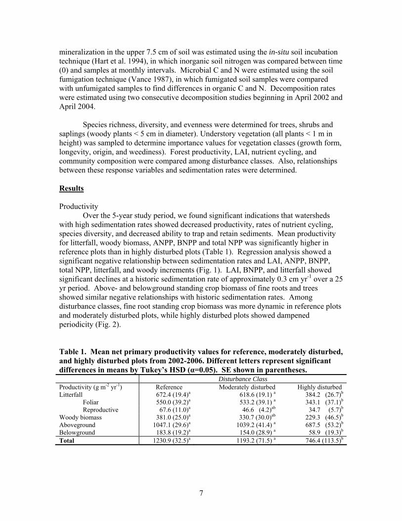
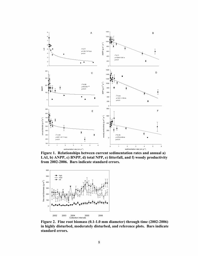
Over the 5-year study period, we found significant indications that watersheds with high sedimentation rates showed decreased productivity, rates of nutrient cycling, species diversity, and decreased ability to trap and retain sediments. Mean productivity for litterfall, woody biomass, ANPP, BNPP and total NPP was significantly higher in reference plots than in highly disturbed plots (Table 1). Regression analysis showed a significant negative relationship between sedimentation rates and LAI, ANPP, BNPP, total NPP, litterfall, and woody increments (Fig. 1). LAI, BNPP, and litterfall showed significant declines at a historic sedimentation rate of approximately 0.3 cm yr-1 over a 25 yr period. Above- and belowground standing crop biomass of fine roots and trees showed similar negative relationships with historic sedimentation rates. Among disturbance classes, fine root standing crop biomass was more dynamic in reference plots and moderately disturbed plots, while highly disturbed plots showed dampened periodicity (Fig. 2). Table 1. Mean net primary productivity values for reference, moderately disturbed, and highly disturbed plots from 2002-2006. Different letters represent significant differences in means by Tukey’s HSD (α=0.05). SE shown in parentheses. Disturbance Class Productivity (g m-2 yr-1) Reference Moderately disturbed Highly disturbed Litterfall 672.4 (19.4)a 618.6 (19.1) a 384.2 (26.7)b

Foliar 550.0 (39.2)a 533.2 (39.1) a 343.1 (37.1)b Reproductive 67.6 (11.0)a 46.6 (4.2)ab 34.7 (5.7)b Woody biomass 381.0 (25.0)a 330.7 (30.0)ab 229.3 (46.5)b

Aboveground 1047.1 (29.6)a 1039.2 (41.4) a 687.5 (53.2)b Belowground 183.8 (19.2)a 154.0 (28.9) a 58.9 (19.3)b Total 1230.9 (32.5)a 1193.2 (71.5) a 746.4 (113.5)b

8

sedimentation rate (cm yr-1)

0 1 2 3 4 5 6

annu

al li

tterfa

ll (g

m-2

yr-1

)

100

200

300

400

500

600

700

800

900

E

r2= 0.49

y=497.1-47.1* ln(x)

p<0.01

BNP

P

0

100

200

300

400

C

r2=0.80y=94.03x-0.20

p<0.01

AN

PP

(g m

-1 y

r-1)

0

200

400

600

800

1000

1200

1400B

r2=0.71

y=1028.6-126.1x

p<0.01

LAI

1

2

3

4

5

6

7

8

9 A

r2=0.77

y=3.36-7.51*ln(x)p<0.01

NP

P (g

m-2

yr-1

)

0

200

400

600

800

1000

1200

1400

1600

D

r2=0.63y=1221.1-159.4x

p<0.01

sedimentation rate (cm yr-1)

0 1 2 3 4 5 6

woo

dy p

rodu

ctiv

ity (g

m-2

yr-1

)

0

200

400

600

800

F

r2=0.35y=378.4-48.4xp<0.01

Figure 1. Relationships between current sedimentation rates and annual a) LAI, b) ANPP, c) BNPP, d) total NPP, e) litterfall, and f) woody productivity from 2002-2006. Bars indicate standard errors.

2002 2003 2004 2005 2006

Collection intervals

fine

root

bio

mas

s (g

m-2

)

0

100

200

300

400

500

600

highmodref

Figure 2. Fine root biomass (0.1-1.0 mm diameter) through time (2002-2006) in highly disturbed, moderately disturbed, and reference plots. Bars indicate standard errors.

9

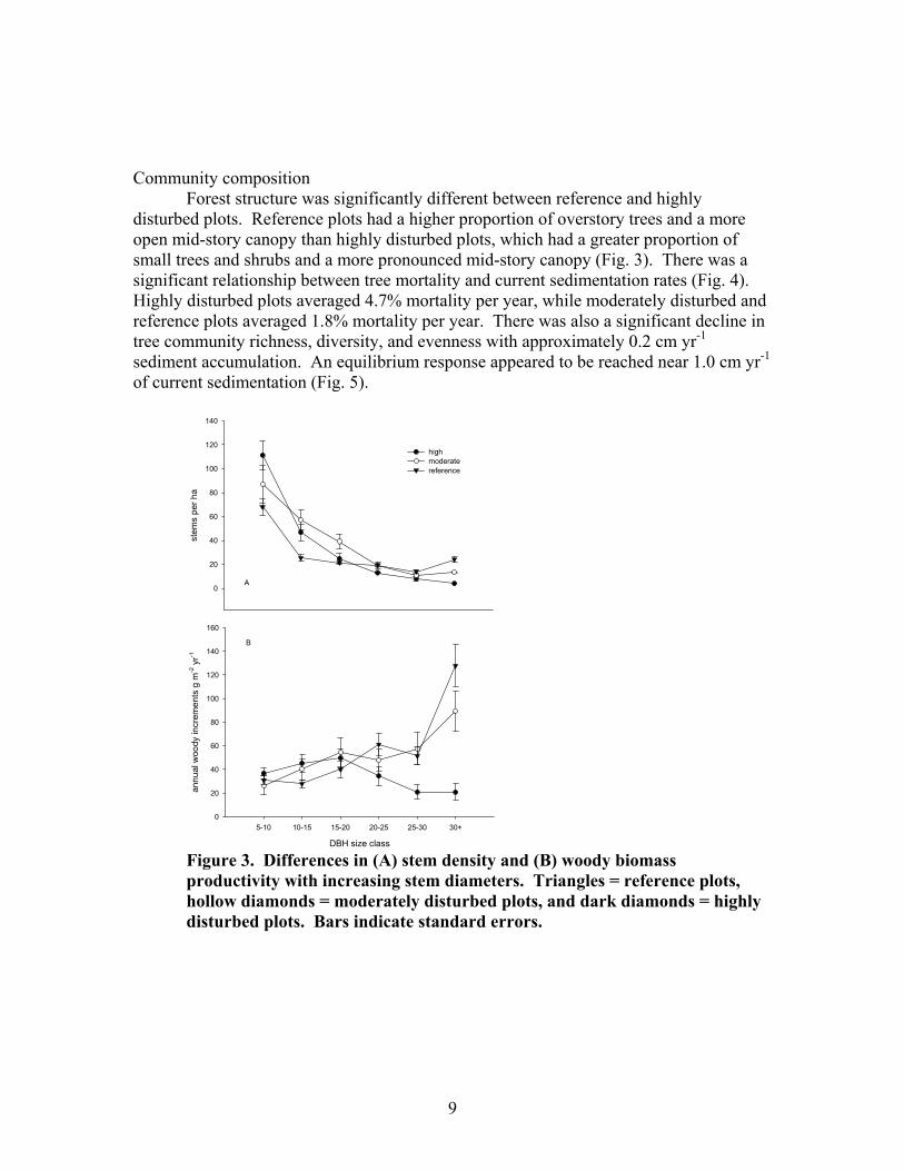
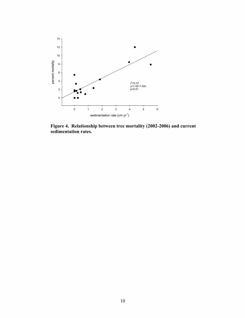
Community composition

Forest structure was significantly different between reference and highly disturbed plots. Reference plots had a higher proportion of overstory trees and a more open mid-story canopy than highly disturbed plots, which had a greater proportion of small trees and shrubs and a more pronounced mid-story canopy (Fig. 3). There was a significant relationship between tree mortality and current sedimentation rates (Fig. 4). Highly disturbed plots averaged 4.7% mortality per year, while moderately disturbed and reference plots averaged 1.8% mortality per year. There was also a significant decline in tree community richness, diversity, and evenness with approximately 0.2 cm yr-1 sediment accumulation. An equilibrium response appeared to be reached near 1.0 cm yr-1 of current sedimentation (Fig. 5).

stem

s pe

r ha

0

20

40

60

80

100

120

140

highmoderatereference

DBH size class

5-10 10-15 15-20 20-25 25-30 30+

annu

al w

oody

incr

emen

ts g

m-2

yr-1

0

20

40

60

80

100

120

140

160

A

B

Figure 3. Differences in (A) stem density and (B) woody biomass productivity with increasing stem diameters. Triangles = reference plots, hollow diamonds = moderately disturbed plots, and dark diamonds = highly disturbed plots. Bars indicate standard errors.

10

sedimentation rate (cm yr-1)

0 1 2 3 4 5 6

perc

ent m

orta

lity

0

2

4

6

8

10

12

14

r2=0.72y=1.42+1.62xp<0.01

Figure 4. Relationship between tree mortality (2002-2006) and current sedimentation rates.

11

spec

ies

richn

ess

(spe

cies

per

ha-1

)

80

100

120

140

160

180

200

220

240

260

r2=0.60y=144.57x-0.09

p<0.01

CSh

anno

n's

dive

rsity

inde

x (H

)

0.8

1.0

1.2

1.4

1.6

1.8

2.0

2.2

r2=0.60y=1.27x-0.06

p<0.01

B

sedimentation rate

0 1 2 3 4 5 6

com

mun

ity e

venn

ess

1.0

1.5

2.0

2.5

3.0

3.5

4.0

4.5

5.0

r2=0.65y=2.24x-0.11

p<0.01

A

Figure 5. Relationships between current sedimentation rates and tree community (A) evenness, (B) diversity, and (C) richness.

12

Shrub and sapling (< 5 cm DBH) biomass increased with current sedimentation rates and reached an equilibrium with approximately 1 cm yr-1 sediment (Fig. 6). Shrub communities did not differ significantly between disturbance classes in terms of diversity, evenness, or richness. There was, however, an increase in N-fixing shrubs (Myrica cerifera and Alnus serrulata) associated with plots receiving higher rates of sediment deposition (Fig. 7).

Understory vegetation (< 1 m in height) comprised only a minor part of the

community composition in most plots. There were no significant differences in understory community richness, evenness, or diversity. Among disturbance classes, annual and exotic species made up a smaller component (i.e. importance value, estimated by frequency and cover) of the understory community in reference plots than in highly disturbed and moderately disturbed plots. Annual species importance exhibited a positive relationship with current sedimentation rates (Fig. 8). There was a strong, positive correlation between percent bare ground and sedimentation rates (r2=0.91, p<0.01).

sedimentation rate (cm yr-1)

0 1 2 3 4 5 6

shru

b bi

omas

s (g

m-2

)

1

2

3

4

5

6

7

8

9

r2=0.44y=5.90 + 0.46ln(x)p<0.01

Figure 6. Relationship between current sedimentation rates and shrub standing crop biomass from 2003-2006. Bars indicate standard errors.

13

sedimentation rate (cm yr-1)

0 1 2 3 4 5 6

log

(den

sity

of N

-fixi

ng s

hrub

s, s

tem

m-2

)

0

1

2

3

4

r2=0.27log Y=1.42+1.62xp<0.01

Figure 7. Relationship between current sedimentation rates and N-fixing shrubs from 2003-2006. Bars indicate standard errors.

sedimentation rate (cm yr-1)

0 1 2 3 4 5 6

natu

ral l

og (R

elat

ive

Impo

rtanc

e Va

lue)

-1.0

-0.5

0.0

0.5

1.0

1.5

2.0

r2=0.22y= 0.33+0.17xp<0.01

Figure 8. Relationship between current sedimentation rates and annual species importance values from 2004-2006. Bars indicate standard errors.

Nutrient cycling

Over the 5 year study period, two consecutive decomposition studies were monitored over a period of 48-64 weeks each. Study 1 began in April 2002 and study 2 in April 2004. Study 1 showed a very significant negative relationship between decomposition rates and historic sedimentation rates (Fig. 9). A rapid decrease in decomposition rates occurred between historic sediment accumulations of 0.2 and 0.3 cm yr-1. Study 2 showed no relationship between decomposition rates and historic sedimentation rates, although there was a strong relationship between current sedimentation rates and percent litter mass and nutrients remaining at the end of 64 weeks

14

(Fig. 10). The differences between these two studies may be due to strong differences in litter quality and precipitation. Poor litter quality and drought conditions in study 1 could have caused the decomposition process to be more sensitive to additional stressors such as sedimentation. Both studies suggest a decline in nutrient cycling rates associated with increased sedimentation.

Figure 9. Relationship between decomposition rates and historical sedimentation rates of foliar litter over 48 weeks. Litter was collected in the fall of 2001 and the study period was from April 2002 to March 2003.

sedimentation rate (cm yr-1)

0 1 2 3 4 5

perc

enta

ge o

f orig

inal

con

tent

0

20

40

60

80

100

120

Mass remaining (r2=0.62, y=11.9+4.6x)N remaining (r2=0.58, y=18.4+11.2x)C remaining (r2=0.75, y=11.9+4.6x)P remaining (r2=0.57, y=18.2+12.7x)

p<0.01

Figure 10. Relationships between current sedimentation rates and mass, N, C, and P remaining in leaf litter after 64 weeks of decomposition. Litterfall was collected in the fall of 2003 and the study period was from April 2004 to July 2005.

-0.07

-0.06

-0.05

-0.04

-0.03

-0.02

-0.01

0

0 1 2 3 4

Sediment (cm yr -1)

k (n

atur

al lo

g of

dec

ay c

oeffi

cien

t)

observed predicted

R2=0.62 Y=-0.06 e-0.00373 (x)

P<0.04

15

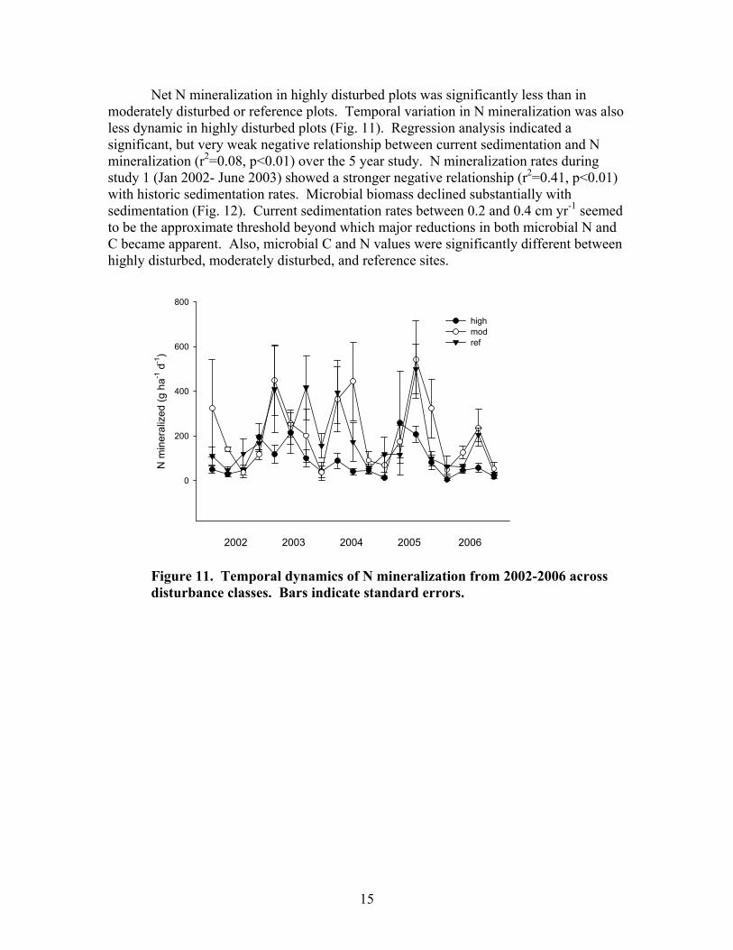
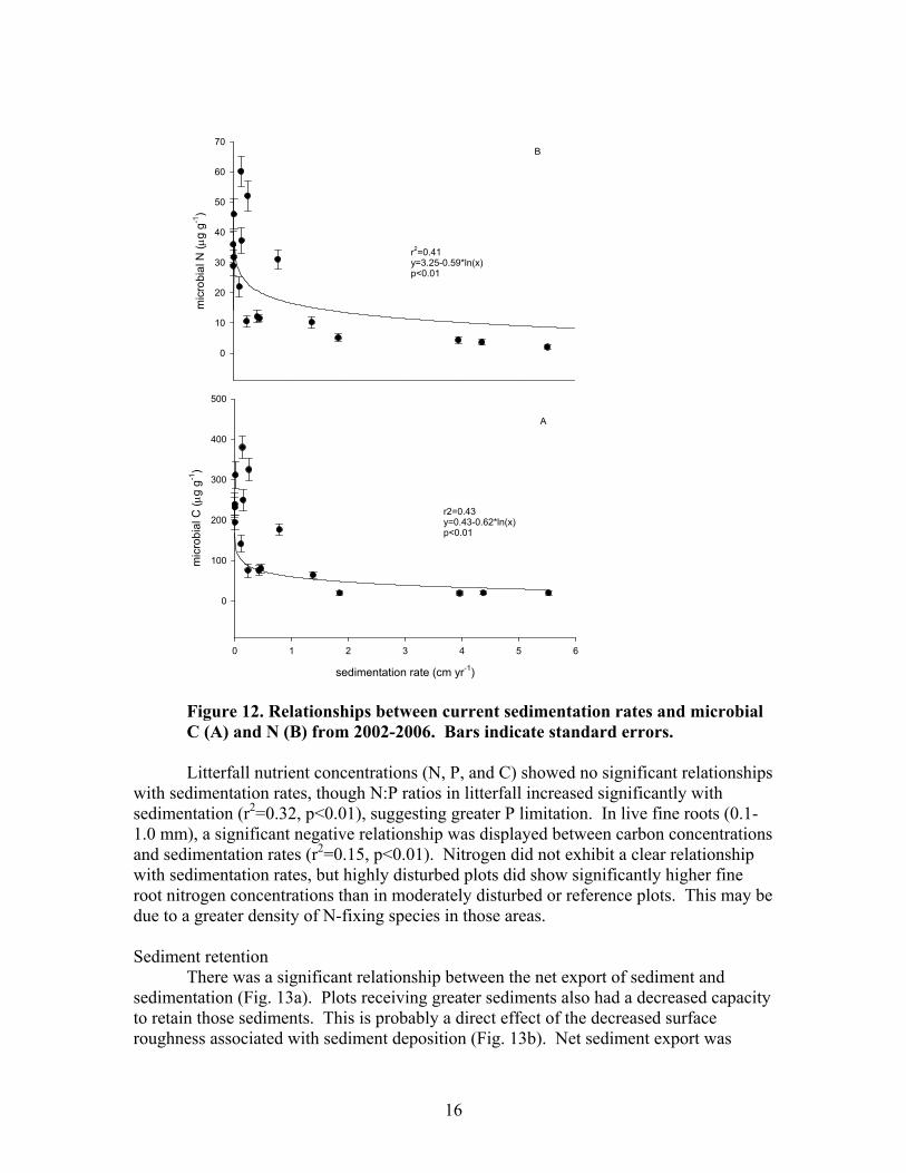
Net N mineralization in highly disturbed plots was significantly less than in moderately disturbed or reference plots. Temporal variation in N mineralization was also less dynamic in highly disturbed plots (Fig. 11). Regression analysis indicated a significant, but very weak negative relationship between current sedimentation and N mineralization (r2=0.08, p<0.01) over the 5 year study. N mineralization rates during study 1 (Jan 2002- June 2003) showed a stronger negative relationship (r2=0.41, p<0.01) with historic sedimentation rates. Microbial biomass declined substantially with sedimentation (Fig. 12). Current sedimentation rates between 0.2 and 0.4 cm yr-1 seemed to be the approximate threshold beyond which major reductions in both microbial N and C became apparent. Also, microbial C and N values were significantly different between highly disturbed, moderately disturbed, and reference sites.

2002 2003 2004 2005 2006

N m

iner

aliz

ed (g

ha-1

d-1

)

0

200

400

600

800

highmodref

Figure 11. Temporal dynamics of N mineralization from 2002-2006 across disturbance classes. Bars indicate standard errors.

16

sedimentation rate (cm yr-1)

0 1 2 3 4 5 6

mic

robi

al C

(μg

g-1)

0

100

200

300

400

500

r2=0.43y=0.43-0.62*ln(x)p<0.01

mic

robi

al N

(μg

g-1)

0

10

20

30

40

50

60

70

r2=0.41y=3.25-0.59*ln(x)p<0.01

A

B

Figure 12. Relationships between current sedimentation rates and microbial C (A) and N (B) from 2002-2006. Bars indicate standard errors. Litterfall nutrient concentrations (N, P, and C) showed no significant relationships

with sedimentation rates, though N:P ratios in litterfall increased significantly with sedimentation (r2=0.32, p<0.01), suggesting greater P limitation. In live fine roots (0.1-1.0 mm), a significant negative relationship was displayed between carbon concentrations and sedimentation rates (r2=0.15, p<0.01). Nitrogen did not exhibit a clear relationship with sedimentation rates, but highly disturbed plots did show significantly higher fine root nitrogen concentrations than in moderately disturbed or reference plots. This may be due to a greater density of N-fixing species in those areas.

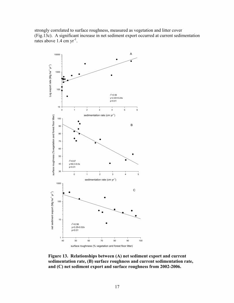
Sediment retention

There was a significant relationship between the net export of sediment and sedimentation (Fig. 13a). Plots receiving greater sediments also had a decreased capacity to retain those sediments. This is probably a direct effect of the decreased surface roughness associated with sediment deposition (Fig. 13b). Net sediment export was

17

strongly correlated to surface roughness, measured as vegetation and litter cover (Fig.13c). A significant increase in net sediment export occurred at current sedimentation rates above 1.4 cm yr-1.

sedimentation rate (cm yr-1)

0 1 2 3 4 5 6

Log

expo

rt ra

te (M

g ha

-1 y

r-1)

10

100

1000

10000 A

r2=0.56y=2.40+0.24xp<0.01

sedimentation rate (cm yr-1)

0 1 2 3 4 5surfa

ce ro

ughn

ess

(%ve

geta

tion

and

fore

st fl

oor l

itter

)

30

40

50

60

70

80

90

100

B

r2=0.67y=84.3-9.0xp<0.01

surface roughness (% vegetation and forest floor litter)

40 50 60 70 80 90 100

net s

edim

ent e

xpor

t (M

g ha

-1 y

r-1)

1

10

100

1000

C

r2=0.56y=3.29-0.02xp<0.01

Figure 13. Relationships between (A) net sediment export and current sedimentation rate, (B) surface roughness and current sedimentation rate, and (C) net sediment export and surface roughness from 2002-2006.

18

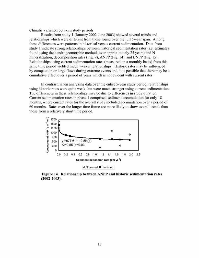
Climatic variation between study periods

Results from study 1 (January 2002-June 2003) showed several trends and relationships which were different from those found over the full 5-year span. Among these differences were patterns in historical versus current sedimentation. Data from study 1 indicate strong relationships between historical sedimentation rates (i.e. estimates found using the dendrogeomorphic method, over approximately 25 years) and N mineralization, decomposition rates (Fig. 9), ANPP (Fig. 14), and BNPP (Fig. 15). Relationships using current sedimentation rates (measured on a monthly basis) from this same time period yielded much weaker relationships. Historic rates may be influenced by compaction or large flows during extreme events and, it is possible that there may be a cumulative effect over a period of years which is not evident with current rates.

In contrast, when analyzing data over the entire 5-year study period, relationships

using historic rates were quite weak, but were much stronger using current sedimentation. The differences in these relationships may be due to differences in study duration. Current sedimentation rates in phase 1 comprised sediment accumulation for only 18 months, where current rates for the overall study included accumulation over a period of 60 months. Rates over the longer time frame are more likely to show overall trends than those from a relatively short time period.

0250500750

1000125015001750

0.0 0.2 0.4 0.6 0.8 1.0 1.2 1.4 1.6 1.8 2.0 2.2

Sediment deposition rate (cm yr-1)

Abo

vegr

ound

NPP

(g m

-2 y

r-1)

Observed Predicted

y =677.6 - 112.5ln(x)r2=0.55 p=0.03

Figure 14. Relationship between ANPP and historic sedimentation rates (2002-2003).

19

Sediment deposition rate (cm yr -1)

0.0 0.5 1.0 1.5 2.0 2.5

Fine

root

NP

P (g

m-2

yr -

1 )

0

200

400

600

800

1000

ObservedPredicted

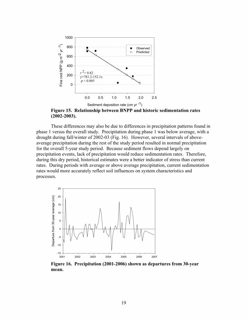
r 2= 0.82y=781.2-152.1x p < 0.005

Figure 15. Relationship between BNPP and historic sedimentation rates (2002-2003). These differences may also be due to differences in precipitation patterns found in

phase 1 versus the overall study. Precipitation during phase 1 was below average, with a drought during fall/winter of 2002-03 (Fig. 16). However, several intervals of above-average precipitation during the rest of the study period resulted in normal precipitation for the overall 5-year study period. Because sediment flows depend largely on precipitation events, lack of precipitation would reduce sedimentation rates. Therefore, during this dry period, historical estimates were a better indicator of stress than current rates. During periods with average or above average precipitation, current sedimentation rates would more accurately reflect soil influences on system characteristics and processes.

2001 2002 2003 2004 2005 2006 2007

Dep

artu

re fr

om 3

0-ye

ar a

vera

ge (c

m)

-15

-10

-5

0

5

10

15

20

25

Figure 16. Precipitation (2001-2006) shown as departures from 30-year mean.

20

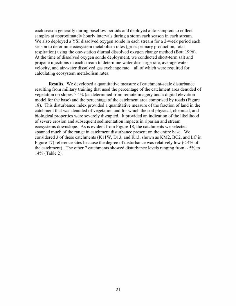
Task 2. Stream Chemistry and Ecosystem Metabolism: Technical Approach. To study the effects of disturbance on stream chemistry and ecosystem metabolism in phase 1 of the project, we used a catchment-scale approach. Eleven study catchments were initially selected, including 3 reference catchments with no discernable current disturbance and 8 disturbed catchments that include a range of apparent disturbance levels (Figure 17). However, the perennial stream in one of our disturbed catchments (D6) went dry during the late spring of 2002, probably as a consequence of the long-term drought. Because this might confound our analysis of effects of disturbance due to military training activities, we were forced to abandon this site, leaving 10 streams for the Phase 1 analysis.

Figure 17. Map showing the 10 study catchments located on the Fort Benning Military Reservation near Columbus, Georgia. Study catchments include two tributaries of Bonham Creek, (BC1, BC2), three tributaries of Sally Branch Creek (SB2, SB3, and SB4), two tributaries of Kings Mill Creek (KM1, KM2), one tributary of Little Pine Knot Creek (LPK); Hollis Branch Creek (HB), and Lois Creek (LC).

Our measurements of stream chemistry and metabolism were made in each of four seasons each year. We collected water chemistry samples from each stream twice

21

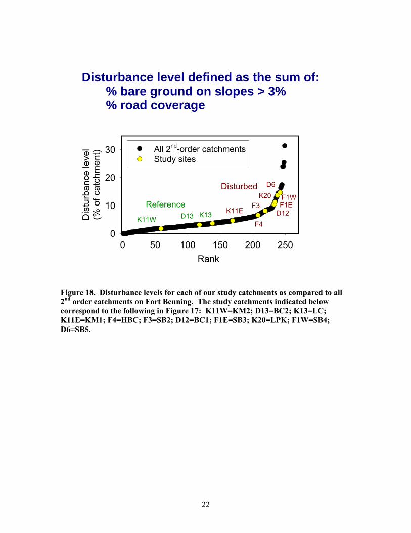
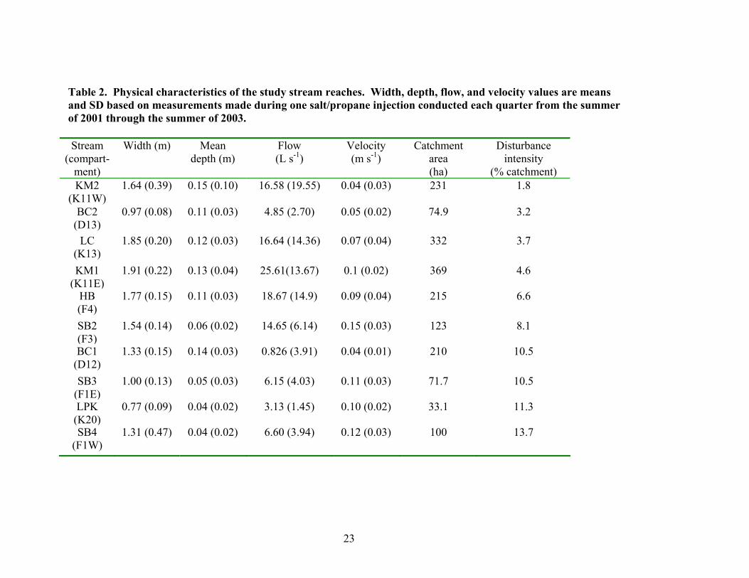
each season generally during baseflow periods and deployed auto-samplers to collect samples at approximately hourly intervals during a storm each season in each stream. We also deployed a YSI dissolved oxygen sonde in each stream for a 2-week period each season to determine ecosystem metabolism rates (gross primary production, total respiration) using the one-station diurnal dissolved oxygen change method (Bott 1996). At the time of dissolved oxygen sonde deployment, we conducted short-term salt and propane injections in each stream to determine water discharge rate, average water velocity, and air-water dissolved gas exchange rate—all of which were required for calculating ecosystem metabolism rates. Results. We developed a quantitative measure of catchment-scale disturbance resulting from military training that used the percentage of the catchment area denuded of vegetation on slopes > 4% (as determined from remote imagery and a digital elevation model for the base) and the percentage of the catchment area comprised by roads (Figure 18). This disturbance index provided a quantitative measure of the fraction of land in the catchment that was denuded of vegetation and for which the soil physical, chemical, and biological properties were severely disrupted. It provided an indication of the likelihood of severe erosion and subsequent sedimentation impacts in riparian and stream ecosystems downslope. As is evident from Figure 18, the catchments we selected spanned much of the range in catchment disturbance present on the entire base. We considered 3 of these catchments (K11W, D13, and K13, shown as KM2, BC2, and LC in Figure 17) reference sites because the degree of disturbance was relatively low (< 4% of the catchment). The other 7 catchments showed disturbance levels ranging from ~ 5% to 14% (Table 2).

22

Figure 18. Disturbance levels for each of our study catchments as compared to all 2nd order catchments on Fort Benning. The study catchments indicated below correspond to the following in Figure 17: K11W=KM2; D13=BC2; K13=LC; K11E=KM1; F4=HBC; F3=SB2; D12=BC1; F1E=SB3; K20=LPK; F1W=SB4; D6=SB5.

Rank 0 50 100 150 200 250

Dis

turb

ance

leve

l(%

of c

atch

men

t)

0

10

20

30 All 2nd-order catchmentsStudy sites

K11WK13D13

K11E

F4

F1ED12

F3K20 F1W

D6

Reference

Disturbed

Disturbance level defined as the sum of: % bare ground on slopes > 3% % road coverage

23

Table 2. Physical characteristics of the study stream reaches. Width, depth, flow, and velocity values are means and SD based on measurements made during one salt/propane injection conducted each quarter from the summer of 2001 through the summer of 2003. Stream

(compart-ment)

Width (m) Mean depth (m)

Flow (L s-1)

Velocity (m s-1)

Catchment area (ha)

Disturbance intensity

(% catchment) KM2

(K11W) 1.64 (0.39) 0.15 (0.10) 16.58 (19.55) 0.04 (0.03) 231 1.8

BC2 (D13)

0.97 (0.08) 0.11 (0.03) 4.85 (2.70) 0.05 (0.02) 74.9 3.2

LC (K13)

1.85 (0.20) 0.12 (0.03) 16.64 (14.36) 0.07 (0.04) 332 3.7

KM1 (K11E)

1.91 (0.22) 0.13 (0.04) 25.61(13.67) 0.1 (0.02) 369 4.6

HB (F4)

1.77 (0.15) 0.11 (0.03) 18.67 (14.9) 0.09 (0.04) 215 6.6

SB2 (F3)

1.54 (0.14) 0.06 (0.02) 14.65 (6.14) 0.15 (0.03) 123 8.1

BC1 (D12)

1.33 (0.15) 0.14 (0.03) 0.826 (3.91) 0.04 (0.01) 210 10.5

SB3 (F1E)

1.00 (0.13) 0.05 (0.03) 6.15 (4.03) 0.11 (0.03) 71.7 10.5

LPK (K20)

0.77 (0.09) 0.04 (0.02) 3.13 (1.45) 0.10 (0.02) 33.1 11.3

SB4 (F1W)

1.31 (0.47) 0.04 (0.02) 6.60 (3.94) 0.12 (0.03) 100 13.7

24

Stream chemistry-Baseflow. The following is a summary of the most important results of Phase 1 work identifying the effects of catchment disturbance on stream chemistry.

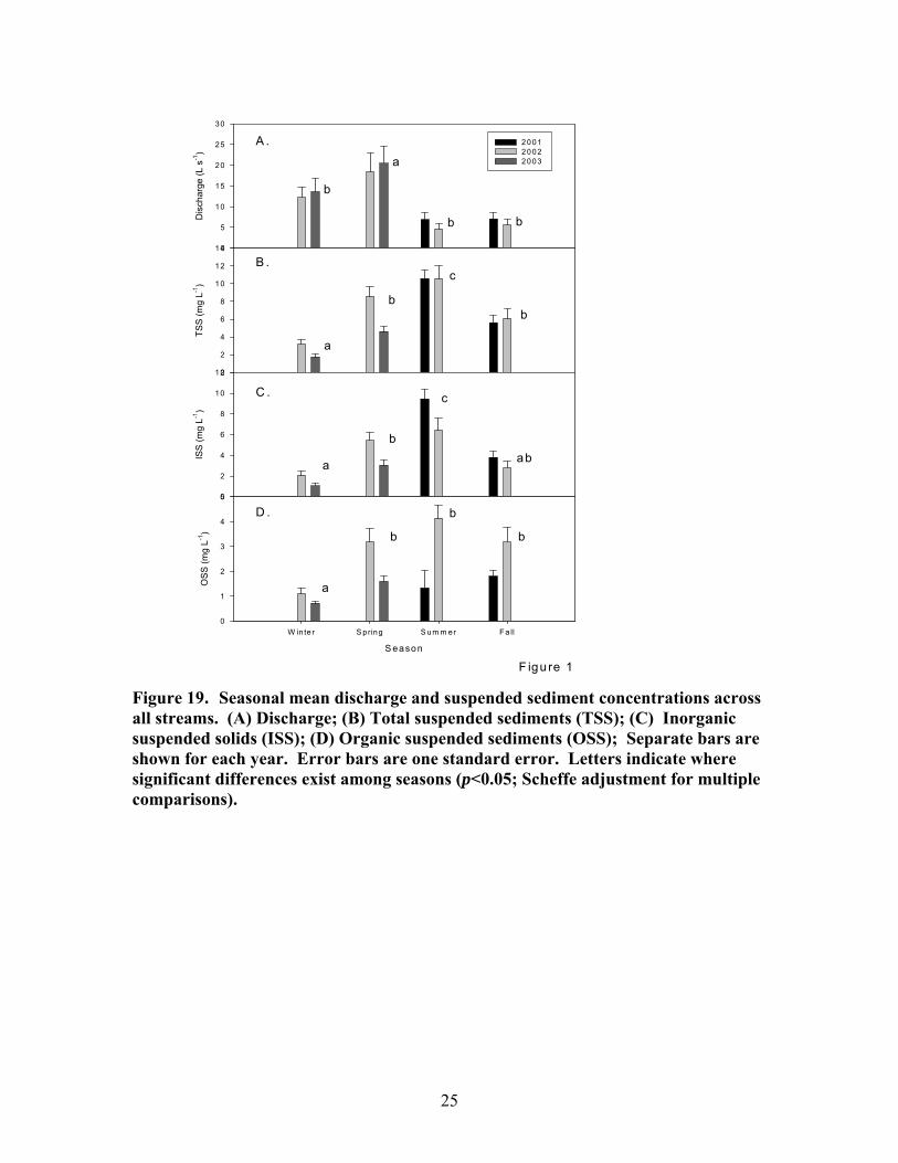
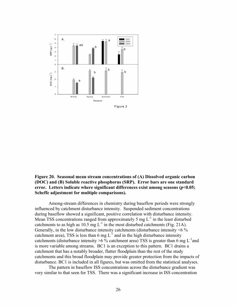
There were moderate seasonal differences in stream discharge and concentrations of suspended sediments, dissolved carbon and nutrients. Maximum stream discharge occurred in spring and minimum stream discharge occurred in summer and fall (Fig 19A). Spring discharge was significantly different from all other seasons. The differences among the other seasons were not significant. The seasonal differences in suspended sediments did not show a clear relationship to seasonal differences in discharge. Minimum suspended sediments (TSS, OSS, and ISS) occurred in winter (Fig 19B-D; Fig 20A), which was a period of intermediate discharge in these streams. The maximum TSS and ISS concentrations occurred in summer, the period of minimum discharge. TSS and ISS were significantly higher in summer than in other seasons. There was not a significant difference in OSS among spring, summer, and fall. OSS concentrations in spring, summer, and fall of 2002 were generally much higher than in 2001 and 2003. Seasonal patterns in DOC concentration were similar to those of OSS concentrations. Minimum DOC concentrations occurred in winter and there were no significant differences among spring, summer and fall DOC concentrations (Fig 20A). Maximum SRP concentration occurred in summer; minimum SRP concentration occurred in spring and fall; and winter was intermediate (Fig 20B). There were no significant seasonal patterns in NH4, NO3, conductivity, pH, or DIN.

25

Dis

char

ge (L

s-1

)

0

5

10

15

20

25

30

2001 2002 2003

TSS

(mg

L-1)

0

2

4

6

8

10

12

14

F igu re 1

A .

B .

a

b

b b

a

b

c

b

ISS

(mg

L-1)

0

2

4

6

8

10

12

C .

a

b

c

ab

S eason

W inte r S pring S um m er F a ll

OSS

(mg

L-1)

0

1

2

3

4

5

D .

a

b

b

b

Figure 19. Seasonal mean discharge and suspended sediment concentrations across all streams. (A) Discharge; (B) Total suspended sediments (TSS); (C) Inorganic suspended solids (ISS); (D) Organic suspended sediments (OSS); Separate bars are shown for each year. Error bars are one standard error. Letters indicate where significant differences exist among seasons (p<0.05; Scheffe adjustment for multiple comparisons).

26

SRP

(ug

L-1)

0

1

2

3

4

5

6

7

2001 2002 2003

S eason

W in ter S pring S um m er Fall

DO

C (m

g L-1

)

0

1

2

3

F igure 2

A .

B .

abb

a

b

a

bb

b

Figure 20. Seasonal mean stream concentrations of (A) Dissolved organic carbon (DOC) and (B) Soluble reactive phosphorus (SRP). Error bars are one standard error. Letters indicate where significant differences exist among seasons (p<0.05; Scheffe adjustment for multiple comparisons).

Among-stream differences in chemistry during baseflow periods were strongly

influenced by catchment disturbance intensity. Suspended sediment concentrations during baseflow showed a significant, positive correlation with disturbance intensity. Mean TSS concentrations ranged from approximately 5 mg L-1 in the least disturbed catchments to as high as 10.5 mg L-1 in the most disturbed catchments (Fig. 21A). Generally, in the low disturbance intensity catchments (disturbance intensity <6 % catchment area), TSS is less than 6 mg L-1 and in the high disturbance intensity catchments (disturbance intensity >6 % catchment area) TSS is greater than 6 mg L-1and is more variable among streams. BC1 is an exception to this pattern. BC1 drains a catchment that has a notably broader, flatter floodplain than the rest of the study catchments and this broad floodplain may provide greater protection from the impacts of disturbance. BC1 is included in all figures, but was omitted from the statistical analyses.

The pattern in baseflow ISS concentrations across the disturbance gradient was very similar to that seen for TSS. There was a significant increase in ISS concentration

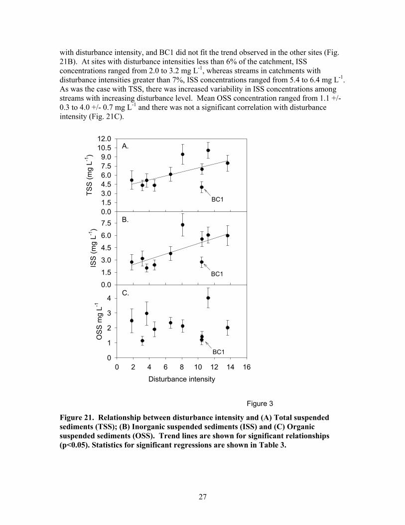
27

with disturbance intensity, and BC1 did not fit the trend observed in the other sites (Fig. 21B). At sites with disturbance intensities less than 6% of the catchment, ISS concentrations ranged from 2.0 to 3.2 mg L-1, whereas streams in catchments with disturbance intensities greater than 7%, ISS concentrations ranged from 5.4 to 6.4 mg L-1. As was the case with TSS, there was increased variability in ISS concentrations among streams with increasing disturbance level. Mean OSS concentration ranged from 1.1 +/- 0.3 to 4.0 +/- 0.7 mg L-1 and there was not a significant correlation with disturbance intensity (Fig. 21C).

ISS

(mg

L-1)

0.0

1.5

3.0

4.5

6.0

7.5

Disturbance intensity

0 2 4 6 8 10 12 14 16

OS

S m

g L-1

0

1

2

3

4

TSS

(mg

L-1)

0.01.53.04.56.07.59.0

10.512.0

BC1

BC1

BC1

Figure 3

A.

B.

C.

Figure 21. Relationship between disturbance intensity and (A) Total suspended sediments (TSS); (B) Inorganic suspended sediments (ISS) and (C) Organic suspended sediments (OSS). Trend lines are shown for significant relationships (p<0.05). Statistics for significant regressions are shown in Table 3.

28

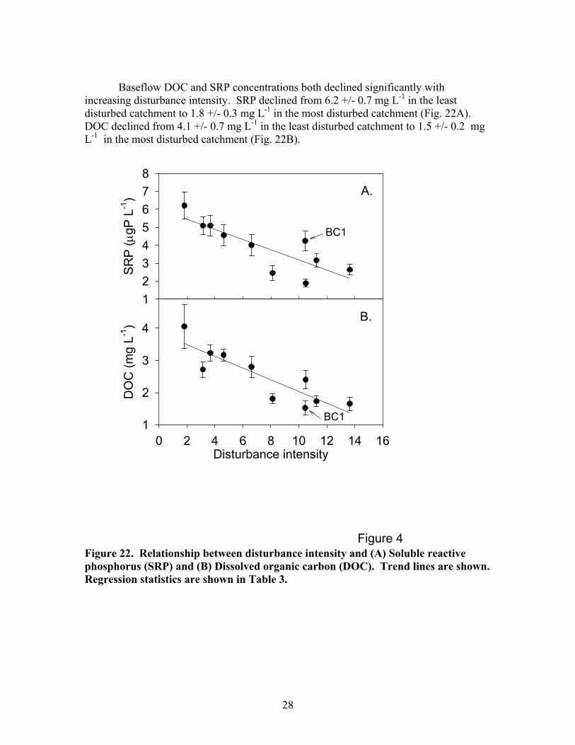
Baseflow DOC and SRP concentrations both declined significantly with

increasing disturbance intensity. SRP declined from 6.2 +/- 0.7 mg L-1 in the least disturbed catchment to 1.8 +/- 0.3 mg L-1 in the most disturbed catchment (Fig. 22A). DOC declined from 4.1 +/- 0.7 mg L-1 in the least disturbed catchment to 1.5 +/- 0.2 mg L-1 in the most disturbed catchment (Fig. 22B).

SRP

(μgP

L-1

)

12345678

Disturbance intensity0 2 4 6 8 10 12 14 16

DO

C (m

g L-1

)

1

2

3

4

A.

B.

Figure 4

BC1

BC1

Figure 22. Relationship between disturbance intensity and (A) Soluble reactive phosphorus (SRP) and (B) Dissolved organic carbon (DOC). Trend lines are shown. Regression statistics are shown in Table 3.

29

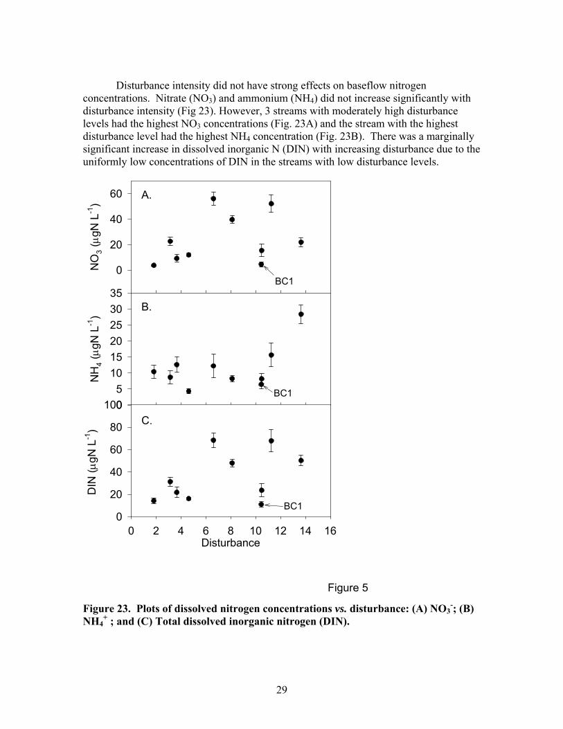
Disturbance intensity did not have strong effects on baseflow nitrogen

concentrations. Nitrate (NO3) and ammonium (NH4) did not increase significantly with disturbance intensity (Fig 23). However, 3 streams with moderately high disturbance levels had the highest NO3 concentrations (Fig. 23A) and the stream with the highest disturbance level had the highest NH4 concentration (Fig. 23B). There was a marginally significant increase in dissolved inorganic N (DIN) with increasing disturbance due to the uniformly low concentrations of DIN in the streams with low disturbance levels.

NO

3 (μ g

N L

-1)

0

20

40

60

NH

4 (μ g

N L

-1)

05

101520253035

Disturbance0 2 4 6 8 10 12 14 16

DIN

(μgN

L-1

)

0

20

40

60

80

100C.

B.

A.

Figure 5

BC1

BC1

BC1

Figure 23. Plots of dissolved nitrogen concentrations vs. disturbance: (A) NO3

-; (B) NH4

+ ; and (C) Total dissolved inorganic nitrogen (DIN).

30

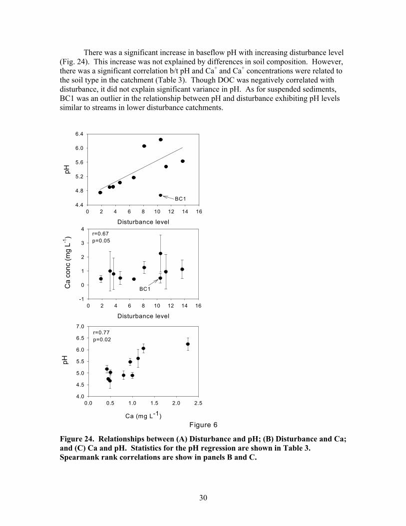
There was a significant increase in baseflow pH with increasing disturbance level (Fig. 24). This increase was not explained by differences in soil composition. However, there was a significant correlation b/t pH and Ca+ and Ca+ concentrations were related to the soil type in the catchment (Table 3). Though DOC was negatively correlated with disturbance, it did not explain significant variance in pH. As for suspended sediments, BC1 was an outlier in the relationship between pH and disturbance exhibiting pH levels similar to streams in lower disturbance catchments.

Disturbance level

0 2 4 6 8 10 12 14 16

pH

4.4

4.8

5.2

5.6

6.0

6.4

Disturbance level

0 2 4 6 8 10 12 14 16

Ca

conc

(mg

L-1)

-1

0

1

2

3

4

Ca (mg L-1)

0.0 0.5 1.0 1.5 2.0 2.5

pH

4.0

4.5

5.0

5.5

6.0

6.5

7.0

Figure 6

r=0.67p=0.05

r=0.77p=0.02

BC1

BC1

Figure 24. Relationships between (A) Disturbance and pH; (B) Disturbance and Ca; and (C) Ca and pH. Statistics for the pH regression are shown in Table 3. Spearmank rank correlations are show in panels B and C.

31

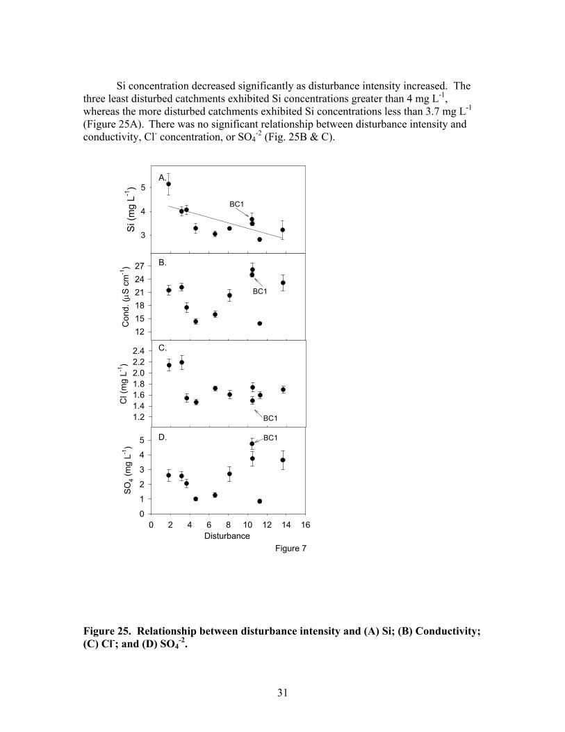
Si concentration decreased significantly as disturbance intensity increased. The

three least disturbed catchments exhibited Si concentrations greater than 4 mg L-1, whereas the more disturbed catchments exhibited Si concentrations less than 3.7 mg L-1 (Figure 25A). There was no significant relationship between disturbance intensity and conductivity, Cl- concentration, or SO4

-2 (Fig. 25B & C).

Si (

mg

L-1)

3

4

5

Cl (

mg

L-1)

1.21.41.61.82.02.22.4

Con

d. (μ

S cm

-1)

121518212427

Disturbance 0 2 4 6 8 10 12 14 16

SO4 (

mg

L-1)

0

1

2

3

4

5

BC1

BC1

BC1

A.

B.

C.

D.

Figure 7

BC1

Figure 25. Relationship between disturbance intensity and (A) Si; (B) Conductivity; (C) Cl-; and (D) SO4

-2.

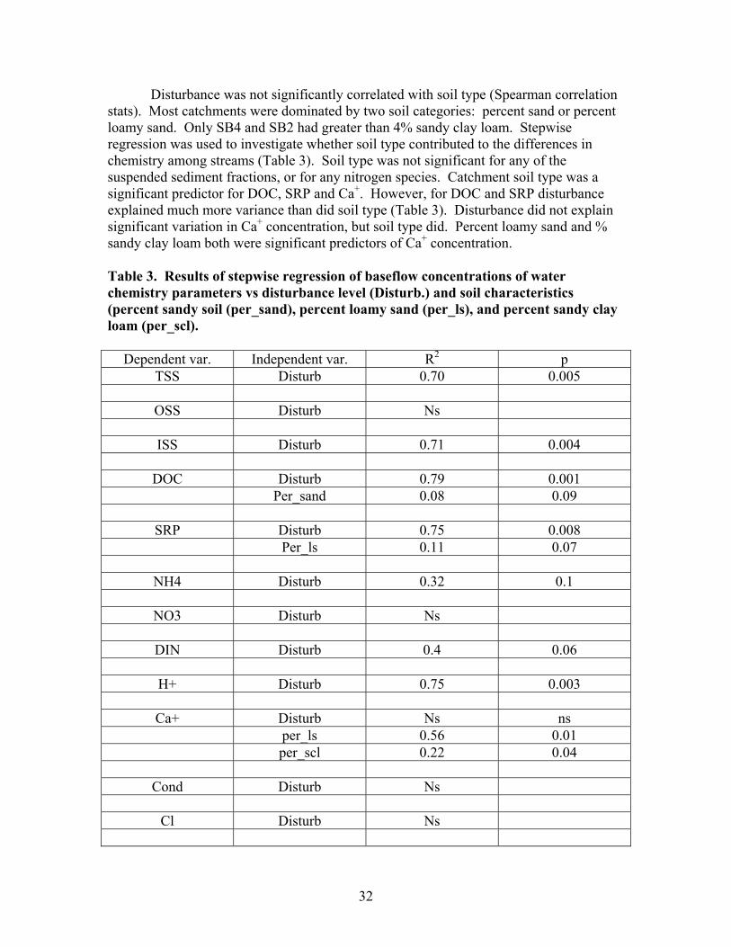
32

Disturbance was not significantly correlated with soil type (Spearman correlation stats). Most catchments were dominated by two soil categories: percent sand or percent loamy sand. Only SB4 and SB2 had greater than 4% sandy clay loam. Stepwise regression was used to investigate whether soil type contributed to the differences in chemistry among streams (Table 3). Soil type was not significant for any of the suspended sediment fractions, or for any nitrogen species. Catchment soil type was a significant predictor for DOC, SRP and Ca+. However, for DOC and SRP disturbance explained much more variance than did soil type (Table 3). Disturbance did not explain significant variation in Ca+ concentration, but soil type did. Percent loamy sand and % sandy clay loam both were significant predictors of Ca+ concentration. Table 3. Results of stepwise regression of baseflow concentrations of water chemistry parameters vs disturbance level (Disturb.) and soil characteristics (percent sandy soil (per_sand), percent loamy sand (per_ls), and percent sandy clay loam (per_scl).

Dependent var. Independent var. R2 p TSS Disturb 0.70 0.005

OSS Disturb Ns

ISS Disturb 0.71 0.004

DOC Disturb 0.79 0.001

Per_sand 0.08 0.09

SRP Disturb 0.75 0.008 Per_ls 0.11 0.07

NH4 Disturb 0.32 0.1

NO3 Disturb Ns

DIN Disturb 0.4 0.06

H+ Disturb 0.75 0.003

Ca+ Disturb Ns ns per_ls 0.56 0.01 per_scl 0.22 0.04

Cond Disturb Ns

Cl Disturb Ns

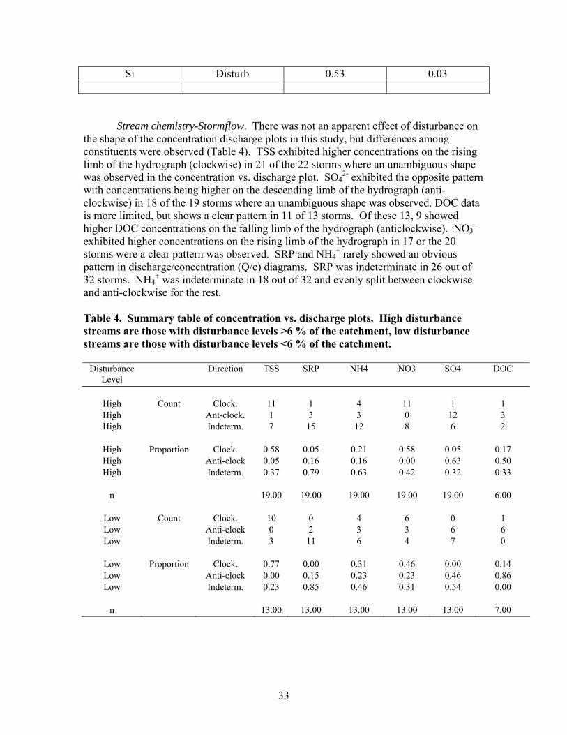
33

Si Disturb 0.53 0.03

Stream chemistry-Stormflow. There was not an apparent effect of disturbance on the shape of the concentration discharge plots in this study, but differences among constituents were observed (Table 4). TSS exhibited higher concentrations on the rising limb of the hydrograph (clockwise) in 21 of the 22 storms where an unambiguous shape was observed in the concentration vs. discharge plot. SO4

2- exhibited the opposite pattern with concentrations being higher on the descending limb of the hydrograph (anti-clockwise) in 18 of the 19 storms where an unambiguous shape was observed. DOC data is more limited, but shows a clear pattern in 11 of 13 storms. Of these 13, 9 showed higher DOC concentrations on the falling limb of the hydrograph (anticlockwise). NO3

- exhibited higher concentrations on the rising limb of the hydrograph in 17 or the 20 storms were a clear pattern was observed. SRP and NH4

+ rarely showed an obvious pattern in discharge/concentration (Q/c) diagrams. SRP was indeterminate in 26 out of 32 storms. NH4

+ was indeterminate in 18 out of 32 and evenly split between clockwise and anti-clockwise for the rest. Table 4. Summary table of concentration vs. discharge plots. High disturbance streams are those with disturbance levels >6 % of the catchment, low disturbance streams are those with disturbance levels <6 % of the catchment.

Disturbance Level

Direction TSS SRP NH4 NO3 SO4 DOC

High Count Clock. 11 1 4 11 1 1 High Ant-clock. 1 3 3 0 12 3 High Indeterm. 7 15 12 8 6 2

High Proportion Clock. 0.58 0.05 0.21 0.58 0.05 0.17 High Anti-clock 0.05 0.16 0.16 0.00 0.63 0.50 High Indeterm. 0.37 0.79 0.63 0.42 0.32 0.33

n 19.00 19.00 19.00 19.00 19.00 6.00

Low Count Clock. 10 0 4 6 0 1 Low Anti-clock 0 2 3 3 6 6 Low Indeterm. 3 11 6 4 7 0

Low Proportion Clock. 0.77 0.00 0.31 0.46 0.00 0.14 Low Anti-clock 0.00 0.15 0.23 0.23 0.46 0.86 Low Indeterm. 0.23 0.85 0.46 0.31 0.54 0.00

n 13.00 13.00 13.00 13.00 13.00 7.00

The impact of disturbance on individual stream chemistry parameters during

storm events was evaluated using the maximum change in concentration during storms (i.e. the difference between baseflow concentration and maximum concentration observed during a storm). The data were not normally distributed and it was not possible to transform the data such that the data or regression residuals were normally distributed. We calculated Spearman rank correlation coefficients to test for significant effects of catchment disturbance on stream chemistry during storms.

The increase in TSS, ISS and OSS during storm events was significantly larger in disturbed catchments. In catchments with a disturbance intensity of < 7% the maximum change in TSS ranged from 57 to 300 mg L-1 (Fig. 26A). In catchments with a disturbance intensity > 7%, maximum change in TSS ranged from 847 to 1881 mg L-1. Also, the variability in maximum change in TSS among storms was also greater for streams with disturbance levels >7% than in streams with lower disturbance levels. As was observed for suspended sediments under baseflow conditions, the pattern in TSS appeared to be driven by the ISS fraction of suspended sediments which showed essentially the same pattern as TSS. In catchments with a disturbance intensity of < 7%, the maximum change in ISS ranged from 38 to 255 mg L-1 (Fig. 26B). In catchments with a disturbance intensity > 7%, maximum change in ISS ranged from 707 to 1378 mg L-1. Again, the variability in maximum change in ISS concentrations among storms was considerably greater in streams draining the more highly disturbed catchments. The maximum change in organic suspended sediments during storm events also increased significantly with disturbance intensity (Fig. 26C). However, the change in OSS was small compared to the change in ISS reflecting the fact that most of the suspended sediments in transport during storms are inorganic. Unlike TSS and ISS, OSS did not show an obvious break point between streams in catchments above and below 7% catchment disturbance. The stream in the second-most disturbed catchment exhibited a much higher maximum change in OSS than any other stream.

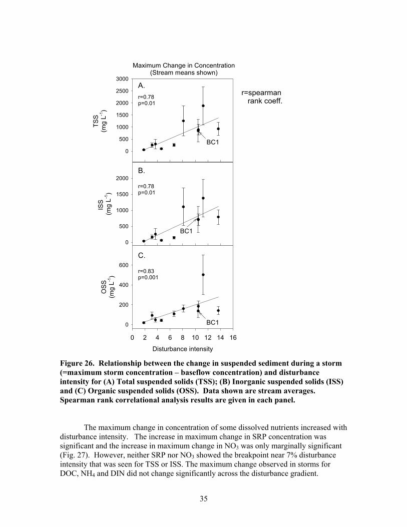
35

ISS

(mg

L-1)

0

500

1000

1500

2000

Disturbance intensity

0 2 4 6 8 10 12 14 16

OSS

(mg

L-1)

0

200

400

600

Maximum Change in Concentration(Stream means shown)

TSS

(mg

L-1)

0

500

1000

1500

2000

2500

3000

r=0.78p=0.01

r=0.83p=0.001

r=0.78p=0.01

r=spearman rank coeff.

A.

B.

C.

BC1

BC1

BC1

Figure 26. Relationship between the change in suspended sediment during a storm (=maximum storm concentration – baseflow concentration) and disturbance intensity for (A) Total suspended solids (TSS); (B) Inorganic suspended solids (ISS) and (C) Organic suspended solids (OSS). Data shown are stream averages. Spearman rank correlational analysis results are given in each panel.

The maximum change in concentration of some dissolved nutrients increased with

disturbance intensity. The increase in maximum change in SRP concentration was significant and the increase in maximum change in NO3 was only marginally significant (Fig. 27). However, neither SRP nor NO3 showed the breakpoint near 7% disturbance intensity that was seen for TSS or ISS. The maximum change observed in storms for DOC, NH4 and DIN did not change significantly across the disturbance gradient.

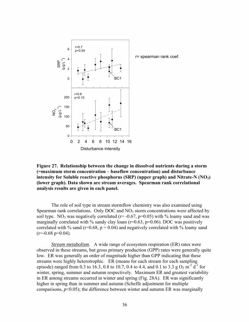
36

Disturbance intensity

0 2 4 6 8 10 12 14 16

NO

3 (μ

g L-1

)

0

50

100

150

200

SR

P(μ

g L-1

)

0

2

4

6

r=0.6p<0.10

r=0.7p=0.04

r= spearman rank coef.

BC1

BC1

Figure 27. Relationship between the change in dissolved nutrients during a storm (=maximum storm concentration – baseflow concentration) and disturbance intensity for Soluble reactive phosphorus (SRP) (upper graph) and Nitrate-N (NO3) (lower graph). Data shown are stream averages. Spearman rank correlational analysis results are given in each panel.

The role of soil type in stream stormflow chemistry was also examined using Spearman rank correlations. Only DOC and NO3 storm concentrations were affected by soil type. NO3 was negatively correlated (r= -0.67, p=0.05) with % loamy sand and was marginally correlated with % sandy clay loam (r=0.63, p=0.06). DOC was positively correlated with % sand (r=0.68, p = 0.04) and negatively correlated with % loamy sand (r=-0.68 p=0.04).

Stream metabolism. A wide range of ecosystem respiration (ER) rates were observed in these streams, but gross primary production (GPP) rates were generally quite low. ER was generally an order of magnitude higher than GPP indicating that these streams were highly heterotrophic. ER (means for each stream for each sampling episode) ranged from 0.3 to 16.3, 0.8 to 10.7, 0.4 to 4.4, and 0.1 to 3.3 g O2 m-2 d-1 for winter, spring, summer and autumn respectively. Maximum ER and greatest variability in ER among streams occurred in winter and spring (Fig. 28A). ER was significantly higher in spring than in summer and autumn (Scheffe adjustment for multiple comparisons, p<0.05); the difference between winter and autumn ER was marginally

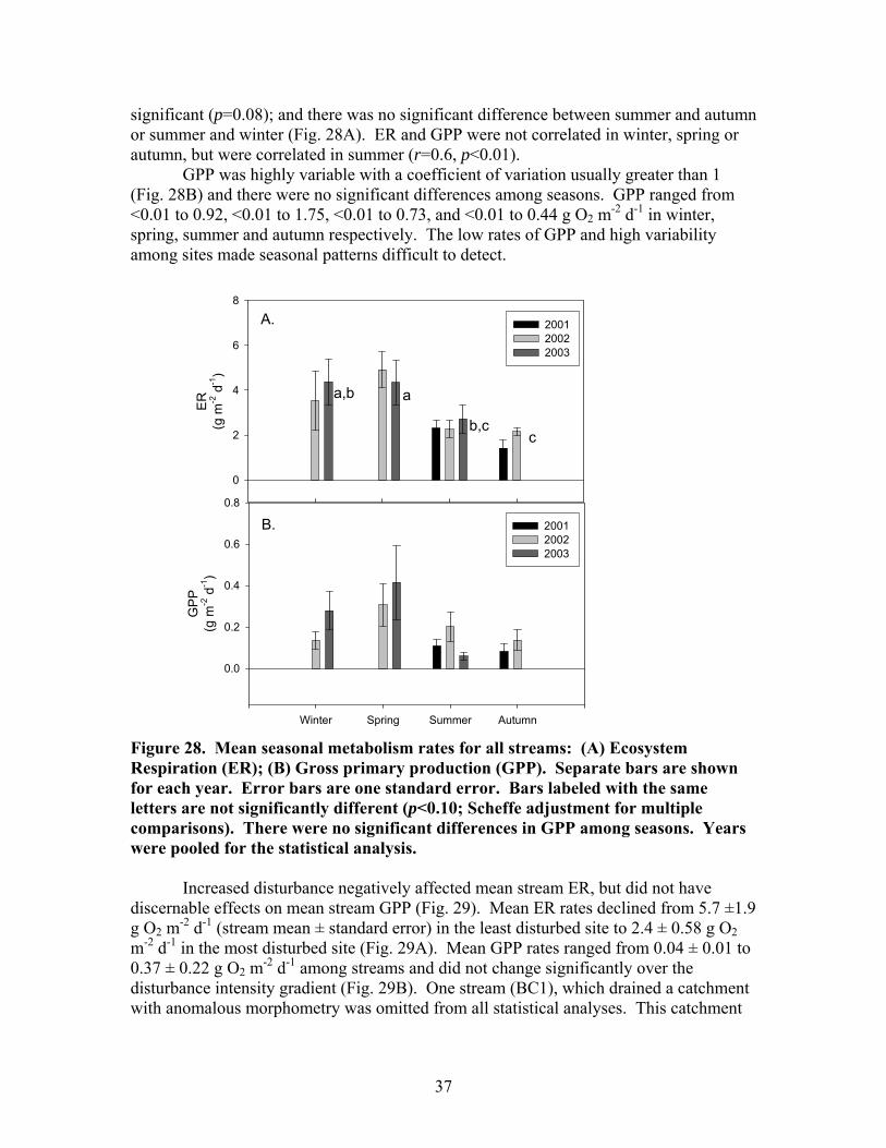
37

significant (p=0.08); and there was no significant difference between summer and autumn or summer and winter (Fig. 28A). ER and GPP were not correlated in winter, spring or autumn, but were correlated in summer (r=0.6, p<0.01).

GPP was highly variable with a coefficient of variation usually greater than 1 (Fig. 28B) and there were no significant differences among seasons. GPP ranged from <0.01 to 0.92, <0.01 to 1.75, <0.01 to 0.73, and <0.01 to 0.44 g O2 m-2 d-1 in winter, spring, summer and autumn respectively. The low rates of GPP and high variability among sites made seasonal patterns difficult to detect.

ER

(g m

-2 d

-1)

0

2

4

6

8

2001 2002 2003

Winter Spring Summer Autumn

GP

P(g

m-2

d-1

)

0.0

0.2

0.4

0.6

0.8

2001 2002 2003

a,b a

b,cc

A.

B.

Figure 28. Mean seasonal metabolism rates for all streams: (A) Ecosystem Respiration (ER); (B) Gross primary production (GPP). Separate bars are shown for each year. Error bars are one standard error. Bars labeled with the same letters are not significantly different (p<0.10; Scheffe adjustment for multiple comparisons). There were no significant differences in GPP among seasons. Years were pooled for the statistical analysis. Increased disturbance negatively affected mean stream ER, but did not have discernable effects on mean stream GPP (Fig. 29). Mean ER rates declined from 5.7 ±1.9 g O2 m-2 d-1 (stream mean ± standard error) in the least disturbed site to 2.4 ± 0.58 g O2 m-2 d-1 in the most disturbed site (Fig. 29A). Mean GPP rates ranged from 0.04 ± 0.01 to 0.37 ± 0.22 g O2 m-2 d-1 among streams and did not change significantly over the disturbance intensity gradient (Fig. 29B). One stream (BC1), which drained a catchment with anomalous morphometry was omitted from all statistical analyses. This catchment

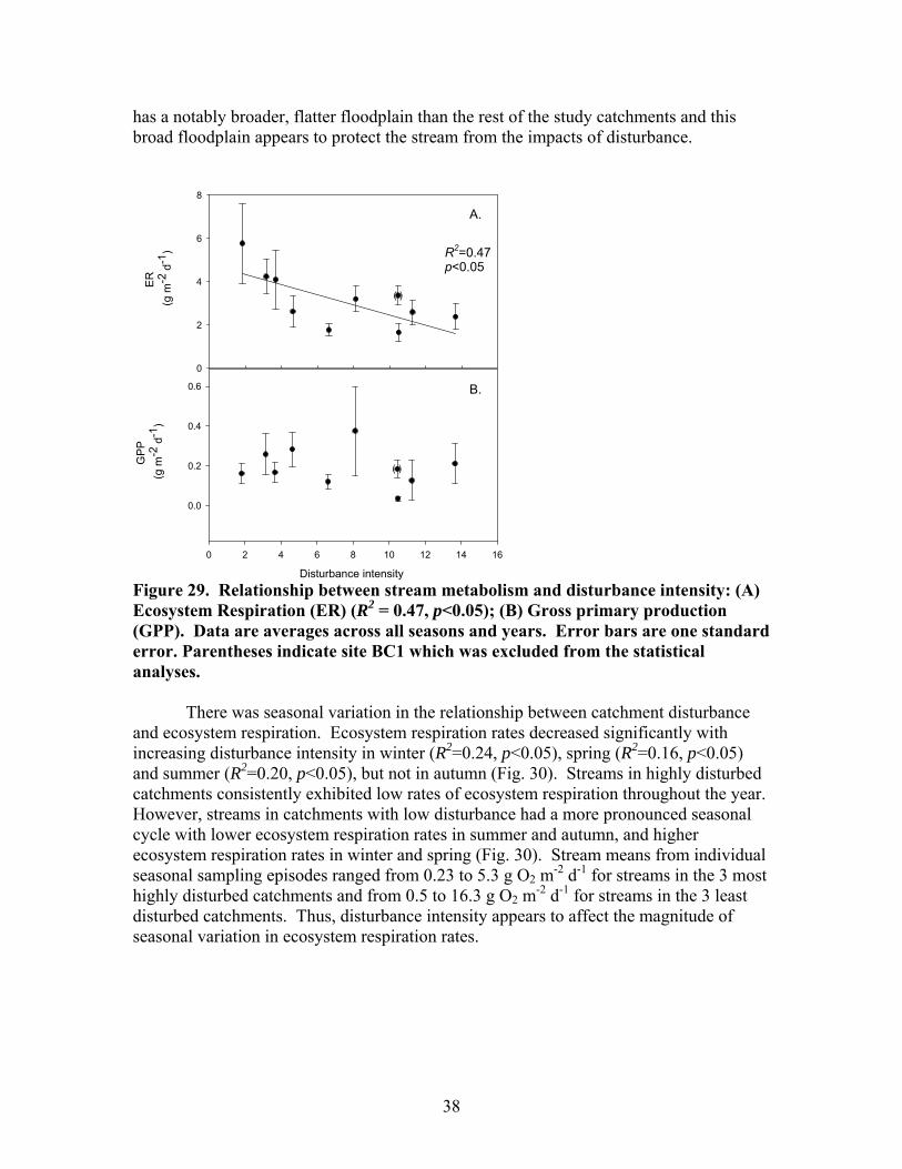
38

has a notably broader, flatter floodplain than the rest of the study catchments and this broad floodplain appears to protect the stream from the impacts of disturbance.

Disturbance intensity

0 2 4 6 8 10 12 14 16

GPP

(g

m-2

d-1

)

0.0

0.2

0.4

0.6

ER

(g m

-2 d

-1)

0

2

4

6

8

( )

( )

R2=0.47p<0.05

A.

B.

Figure 29. Relationship between stream metabolism and disturbance intensity: (A) Ecosystem Respiration (ER) (R2 = 0.47, p<0.05); (B) Gross primary production (GPP). Data are averages across all seasons and years. Error bars are one standard error. Parentheses indicate site BC1 which was excluded from the statistical analyses.

There was seasonal variation in the relationship between catchment disturbance and ecosystem respiration. Ecosystem respiration rates decreased significantly with increasing disturbance intensity in winter (R2=0.24, p<0.05), spring (R2=0.16, p<0.05) and summer (R2=0.20, p<0.05), but not in autumn (Fig. 30). Streams in highly disturbed catchments consistently exhibited low rates of ecosystem respiration throughout the year. However, streams in catchments with low disturbance had a more pronounced seasonal cycle with lower ecosystem respiration rates in summer and autumn, and higher ecosystem respiration rates in winter and spring (Fig. 30). Stream means from individual seasonal sampling episodes ranged from 0.23 to 5.3 g O2 m-2 d-1 for streams in the 3 most highly disturbed catchments and from 0.5 to 16.3 g O2 m-2 d-1 for streams in the 3 least disturbed catchments. Thus, disturbance intensity appears to affect the magnitude of seasonal variation in ecosystem respiration rates.

39

Winter

0369

121518

Spring

02468

1012

Summer

ER

(g m

-2 d

-1)

012345

Autumn

Disturbance intensity0 2 4 6 8 10 12 14 16

0

1

2

3

R2=0.16 p<0.05

R2=0.24 p<0.05

R2=0.20 p<0.05

( )( )

( )

( )

( )

( )

( )

200120022003

( )( )

Figure 30. Ecosystem respiration (ER) vs. disturbance intensity for each season. Seasonal means for each year are shown as separate points. Regression analyses within each season were performed for all years combined. Regression lines are plotted for relationships that are significant at p<0.05 (Table 5).

When analyzed by season, there was no significant relationship between GPP and disturbance (Fig. 31), unlike ecosystem respiration. Stream means for individual seasonal sampling episodes ranged from < 0.01 to 0.87 g O2 m-2 d-1 in streams in the 3 most highly disturbed catchments and from <0.01 to 0.96 g O2 m-2 d-1 for streams in the 3 least disturbed catchments. However, separate analysis of spring 2002 data indicated that there was a significant, negative relationship between disturbance and GPP in the spring of 2002.

40

Winter

0.00.20.40.60.81.01.2

Autumn

Disturbance intensity0 2 4 6 8 10 12 14 16

0.0

0.1

0.2

0.3

0.4

Summer

GP

P(g

m-2

d-1

)

0.0

0.1

0.2

0.3

200120022003

Spring

0.0

0.5

1.0

1.5R2=0.51p=0.02

( )( )

( )

( )

( )

( )

(2002 data only)

Figure 31. Gross primary production vs. disturbance intensity for each season. Seasonal means for each year are shown as separate points. Regression line for spring data includes only 2002 data (Table 5). Stepwise multiple regression analysis, conducted separately for each season, was used to examine relationships between stream respiration and 1) disturbance intensity, and 2) stream temperature (Table 5). Disturbance intensity, but not temperature was a significant predictor of stream respiration for winter, spring and summer (Table 5). In contrast, stream temperature, but not disturbance intensity a significant predictor of stream respiration in autumn (Table 5). Similar analysis of the relationships between seasonal mean GPP and 1) disturbance intensity and 2) solar irradiance showed that disturbance intensity was not a significant predictor of GPP at the seasonal scale, but was significant for spring 2002 GPP analyzed separately. Solar irradiance was a significant predictor of GPP in summer and autumn (Table 5). The effect of solar irradiance would likely have been more pronounced had days with solar irradiance <70% of the monthly maximum not been eliminated from analysis.

41

Table 5. Regression analysis results for stream respiration (R) and gross primary production (GPP), by season.

Season Dependent variable

Independent variable

Slope ± s.e. R2 p

Winter Log ER Disturbance -0.088 ± 0.041 0.24 <0.05

Spring Disturbance -0.087 ± 0.041 0.16 0.05

Summer Disturbance -0.11 ± 0.045 0.20 <0.05

Autumn Temperature 0.10 ± 0.037 0.32 <0.05

Spring 2002 Log GPP Disturbance -0.37 ± 0.12 0.51 <0.05

Summer Solar irrad. 0.025 ± 0.11 0.16 <0.05

Autumn Solar irrad. 0.031 ± 0.15 0.18 0.05

Percent benthic organic matter (%BOM) and coarse woody debris (CWD) abundance were also evaluated as potential correlates of ecosystem respiration. Both %BOM and CWD abundance decline significantly as disturbance intensity increases (see section on Stream Habitat and Biota). Because of the high covariance among %BOM, CWD and disturbance, inclusion of more than one of these predictors in the stepwise regression analysis would have been redundant. The relationship between ER and each of these predictors (%BOM and CWD) was quantified by correlational analysis. Mean stream ER was not significantly correlated with mean stream %BOM (Spearman correlation coefficient, r= 0.48 p=0.2; Fig 32A), but was significantly correlated to CWD abundance (r=0.85 p<0.01, Fig 32B).

42

%BOM

0 1 2 3 4 7 8

ER

(g m

-2 d

-1)

0

1

2

3

4

5

6

7

8

CWD

0.04 0.06 0.08 0.10 0.12 0.14 0.16

ER

(g

m-2

d-1

)

0

1

2

3

4

5

6

7

8

A.

B.

Figure 32. (A) Ecosystem respiration (ER) vs. percent benthic organic matter (%BOM; Spearman correlation coeff.=0.47, p=0.2) and (B) ER vs coarse woody debris (CWD; Spearman correlation coeff. = 0.85, p=0.004). CWD was measured as a proportion of stream area (m2 CWD per m2 stream bottom).

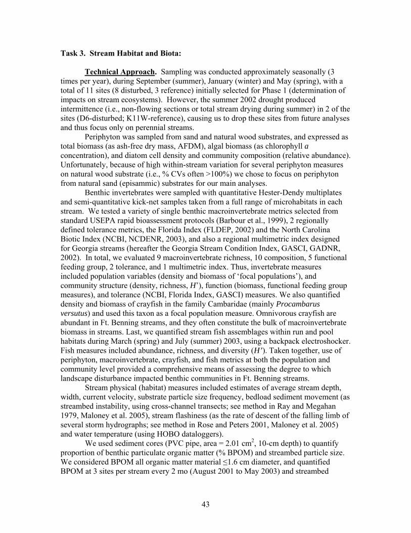
43

Task 3. Stream Habitat and Biota:

Technical Approach. Sampling was conducted approximately seasonally (3 times per year), during September (summer), January (winter) and May (spring), with a total of 11 sites (8 disturbed, 3 reference) initially selected for Phase 1 (determination of impacts on stream ecosystems). However, the summer 2002 drought produced intermittence (i.e., non-flowing sections or total stream drying during summer) in 2 of the sites (D6-disturbed; K11W-reference), causing us to drop these sites from future analyses and thus focus only on perennial streams.

Periphyton was sampled from sand and natural wood substrates, and expressed as total biomass (as ash-free dry mass, AFDM), algal biomass (as chlorophyll a concentration), and diatom cell density and community composition (relative abundance). Unfortunately, because of high within-stream variation for several periphyton measures on natural wood substrate (i.e., % CVs often >100%) we chose to focus on periphyton from natural sand (episammic) substrates for our main analyses.

Benthic invertebrates were sampled with quantitative Hester-Dendy multiplates and semi-quantitative kick-net samples taken from a full range of microhabitats in each stream. We tested a variety of single benthic macroinvertebrate metrics selected from standard USEPA rapid bioassessment protocols (Barbour et al., 1999), 2 regionally defined tolerance metrics, the Florida Index (FLDEP, 2002) and the North Carolina Biotic Index (NCBI, NCDENR, 2003), and also a regional multimetric index designed for Georgia streams (hereafter the Georgia Stream Condition Index, GASCI, GADNR, 2002). In total, we evaluated 9 macroinvertebrate richness, 10 composition, 5 functional feeding group, 2 tolerance, and 1 multimetric index. Thus, invertebrate measures included population variables (density and biomass of ‘focal populations’), and community structure (density, richness, H’), function (biomass, functional feeding group measures), and tolerance (NCBI, Florida Index, GASCI) measures. We also quantified density and biomass of crayfish in the family Cambaridae (mainly Procambarus versutus) and used this taxon as a focal population measure. Omnivorous crayfish are abundant in Ft. Benning streams, and they often constitute the bulk of macroinvertebrate biomass in streams. Last, we quantified stream fish assemblages within run and pool habitats during March (spring) and July (summer) 2003, using a backpack electroshocker. Fish measures included abundance, richness, and diversity (H’). Taken together, use of periphyton, macroinvertebrate, crayfish, and fish metrics at both the population and community level provided a comprehensive means of assessing the degree to which landscape disturbance impacted benthic communities in Ft. Benning streams. Stream physical (habitat) measures included estimates of average stream depth, width, current velocity, substrate particle size frequency, bedload sediment movement (as streambed instability, using cross-channel transects; see method in Ray and Megahan 1979, Maloney et al. 2005), stream flashiness (as the rate of descent of the falling limb of several storm hydrographs; see method in Rose and Peters 2001, Maloney et al. 2005) and water temperature (using HOBO dataloggers). We used sediment cores (PVC pipe, area = 2.01 cm2, 10-cm depth) to quantify proportion of benthic particulate organic matter (% BPOM) and streambed particle size. We considered BPOM all organic matter material ≤1.6 cm diameter, and quantified BPOM at 3 sites per stream every 2 mo (August 2001 to May 2003) and streambed

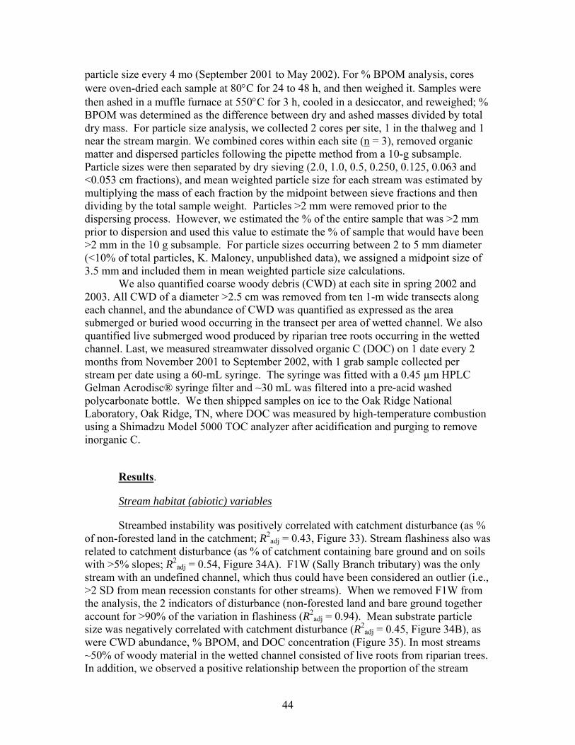
44

particle size every 4 mo (September 2001 to May 2002). For % BPOM analysis, cores were oven-dried each sample at 80°C for 24 to 48 h, and then weighed it. Samples were then ashed in a muffle furnace at 550°C for 3 h, cooled in a desiccator, and reweighed; % BPOM was determined as the difference between dry and ashed masses divided by total dry mass. For particle size analysis, we collected 2 cores per site, 1 in the thalweg and 1 near the stream margin. We combined cores within each site (n = 3), removed organic matter and dispersed particles following the pipette method from a 10-g subsample. Particle sizes were then separated by dry sieving (2.0, 1.0, 0.5, 0.250, 0.125, 0.063 and <0.053 cm fractions), and mean weighted particle size for each stream was estimated by multiplying the mass of each fraction by the midpoint between sieve fractions and then dividing by the total sample weight. Particles >2 mm were removed prior to the dispersing process. However, we estimated the % of the entire sample that was >2 mm prior to dispersion and used this value to estimate the % of sample that would have been >2 mm in the 10 g subsample. For particle sizes occurring between 2 to 5 mm diameter (<10% of total particles, K. Maloney, unpublished data), we assigned a midpoint size of 3.5 mm and included them in mean weighted particle size calculations.

We also quantified coarse woody debris (CWD) at each site in spring 2002 and 2003. All CWD of a diameter >2.5 cm was removed from ten 1-m wide transects along each channel, and the abundance of CWD was quantified as expressed as the area submerged or buried wood occurring in the transect per area of wetted channel. We also quantified live submerged wood produced by riparian tree roots occurring in the wetted channel. Last, we measured streamwater dissolved organic C (DOC) on 1 date every 2 months from November 2001 to September 2002, with 1 grab sample collected per stream per date using a 60-mL syringe. The syringe was fitted with a 0.45 µm HPLC Gelman Acrodisc® syringe filter and ~30 mL was filtered into a pre-acid washed polycarbonate bottle. We then shipped samples on ice to the Oak Ridge National Laboratory, Oak Ridge, TN, where DOC was measured by high-temperature combustion using a Shimadzu Model 5000 TOC analyzer after acidification and purging to remove inorganic C.

Results.

Stream habitat (abiotic) variables

Streambed instability was positively correlated with catchment disturbance (as % of non-forested land in the catchment; R2

adj = 0.43, Figure 33). Stream flashiness also was related to catchment disturbance (as % of catchment containing bare ground and on soils with >5% slopes; R2

adj = 0.54, Figure 34A). F1W (Sally Branch tributary) was the only stream with an undefined channel, which thus could have been considered an outlier (i.e., >2 SD from mean recession constants for other streams). When we removed F1W from the analysis, the 2 indicators of disturbance (non-forested land and bare ground together account for >90% of the variation in flashiness (R2

adj = 0.94). Mean substrate particle size was negatively correlated with catchment disturbance (R2

adj = 0.45, Figure 34B), as were CWD abundance, % BPOM, and DOC concentration (Figure 35). In most streams ~50% of woody material in the wetted channel consisted of live roots from riparian trees. In addition, we observed a positive relationship between the proportion of the stream

45

channel containing submerged CWD and % BPOM (Fig. 36), indicating the potential importance of coarse woody debris in organic matter retention in Ft. Benning streams. Thus, streambed instability, stream flashiness, and all 3 organic matter variables were useful indicators of catchment-scale disturbance in Phase 1. These results have been documented in a paper that was published in Environmental Management (Maloney et al. 2005).

% of catchment as nonforested land

0 10 20 30 40

Stre

ambe

d in

stab

ility

(mm

)

0

2

4

6

8

R2 = 0.50p = 0.033

Figure 33. Relationship between streambed instability, calculated as the mean absolute change in streambed height from January to July 2003, plotted against catchment disturbance, measured as % of nonforested land in study catchments. (Mean ± 1SE) (from Maloney et al. 2005).

46

% Catchment as bare ground and road cover

0 5 10 15

Log

parti

cle

size

(mm

)

-0.3

-0.2

-0.1

0.0

0.1

4-h

rece

ssio

n co

nsta

nt (h

-1)

0.0

0.1

0.2

0.3

0.4

0.5A

B

R2 = 0.87p = 0.001

R2 = 0.51p = 0.014

Figure 34. Stream flashiness (4-h recession constants) calculated as the regression slope of the LN(flow) for 4 h following peak flow as a function of catchment disturbance (% of bare ground in study catchment) (A) and mean stream substrate particle size (B) plotted against the % of bare ground and road cover in a catchment. Triangle indicates outlier catchments (>2 SD below the mean), F1W for recession constant (A) and D12 for particle size (B) that were excluded from analyses. (Mean ± 1SE) (from Maloney et al. 2005).

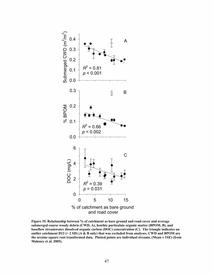
47

Sub

mer

ged

CW

D (m

2 /m2 )

0.0

0.1

0.2

0.3

0.4 A

% B

PO

M

0.0

0.1

0.2

0.3 B

% of catchment as bare ground and road cover

0 5 10 15

DO

C (m

g/L)

0

2

4

6C

R2 = 0.81p < 0.001

R2 = 0.66p = 0.002

R2 = 0.39p = 0.031

Figure 35. Relationship between % of catchment as bare ground and road cover and average submerged coarse woody debris (CWD, A), benthic particulate organic matter (BPOM, B), and baseflow streamwater dissolved organic carbon (DOC) concentration (C). The triangle indicates an outlier catchment D12 (> 2 SD) (A & B only) that was excluded from analyses. CWD and BPOM are the arcsine square root transformed data. Plotted points are individual streams. (Mean ± 1SE) (from Maloney et al. 2005).

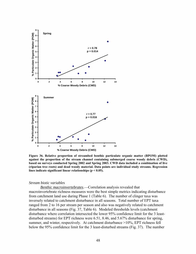
48

Figure 36. Relative proportion of streambed benthic particulate organic matter (BPOM) plotted against the proportion of the stream channel containing submerged coarse woody debris (CWD), based on surveys conducted Spring 2002 and Spring 2003. CWD data included a combination of live (riparian tree roots) and dead woody material. Data points are individual study streams. Regression lines indicate significant linear relationships (p < 0.05).

Stream biotic variables Benthic macroinvertebrates.—Correlation analysis revealed that

macroinvertebrate richness measures were the best simple metrics indicating disturbance from catchment land use during Phase 1 (Table 6). The number of clinger taxa was inversely related to catchment disturbance in all seasons. Total number of EPT taxa ranged from 2 to 16 per stream per season and also was negatively related to catchment disturbance in all seasons (Fig. 37, Table 6). Modeled thresholds levels (catchment disturbance where correlation intersected the lower 95% confidence limit for the 3 least-disturbed streams) for EPT richness were 6.51, 8.46, and 5.67% disturbance for spring, summer, and winter, respectively. At catchment disturbance >10%, EPT richness fell below the 95% confidence limit for the 3 least-disturbed streams (Fig. 37). The number

0

1

2

3

4

5

6

7

8

9

0 2 4 6 8 10 12 14

% Coarse Woody Debris (CWD)

% P

artic

ulat

e O

rgan

ic M

atte

r (PO

M) Summer

r = 0.77 p = 0.016

0

1

2

3

4

5

6

7

8

9

0 2 4 6 8 10 12 14

% Coarse Woody Debris (CWD)

% P

artic

ulat

e O

rgan

ic M

atte

r (PO

M) Spring

r = 0.78p = 0.014

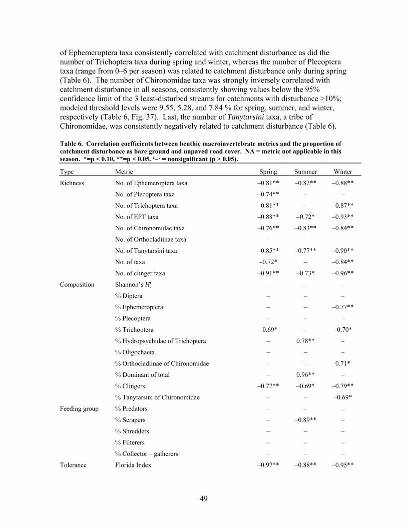
49

of Ephemeroptera taxa consistently correlated with catchment disturbance as did the number of Trichoptera taxa during spring and winter, whereas the number of Plecoptera taxa (range from 0–6 per season) was related to catchment disturbance only during spring (Table 6). The number of Chironomidae taxa was strongly inversely correlated with catchment disturbance in all seasons, consistently showing values below the 95% confidence limit of the 3 least-disturbed streams for catchments with disturbance >10%; modeled threshold levels were 9.55, 5.28, and 7.84 % for spring, summer, and winter, respectively (Table 6, Fig. 37). Last, the number of Tanytarsini taxa, a tribe of Chironomidae, was consistently negatively related to catchment disturbance (Table 6).

Table 6. Correlation coefficients between benthic macroinvertebrate metrics and the proportion of catchment disturbance as bare ground and unpaved road cover. NA = metric not applicable in this season. *=p < 0.10, **=p < 0.05. ‘–‘ = nonsignificant (p > 0.05).

Type Metric Spring Summer Winter

Richness No. of Ephemeroptera taxa –0.81** –0.82** –0.88**

No. of Plecoptera taxa –0.74** – –

No. of Trichoptera taxa –0.81** – –0.87**

No. of EPT taxa –0.88** –0.72* –0.93**

No. of Chironomidae taxa –0.76** –0.83** –0.84**

No. of Orthocladiinae taxa – – –

No. of Tanytarsini taxa –0.85** –0.77** –0.90**

No. of taxa –0.72* – –0.84**

No. of clinger taxa –0.91** –0.73* –0.96**

Composition Shannon’s H' – – –

% Diptera – – –

% Ephemeroptera – – –0.77**

% Plecoptera – – –

% Trichoptera –0.69* – –0.70*

% Hydropsychidae of Trichoptera – 0.78** –

% Oligochaeta – – –

% Orthocladiinae of Chironomidae – – 0.71*

% Dominant of total – 0.96** –

% Clingers –0.77** –0.69* –0.79**

% Tanytarsini of Chironomidae – – –0.69*

Feeding group % Predators – – –

% Scrapers – –0.89** –

% Shredders – – –

% Filterers – – –

% Collector – gatherers – – –

Tolerance Florida Index –0.97** –0.88** –0.95**

50

NCBI – – 0.71*

Multimetric GASCI NA –0.96** –0.95**

spring

Num

ber o

f E

PT

taxa

0

5

10

15

20

summer winter

Num

ber o

f C

hiro

nom

idae

taxa

0

5

10

15

20

25

30

0 5 10 15

Flor

ida

inde

x

0

5

10

15

20

25

30

% of catchment as bare ground and unpaved roads0 5 10 15 0 5 10 15

(2)

(2)

(2)(2)

(2)

(2) (2)

(2)

(2)(2)

(2)

(2)(2)(3)

(2)

(2)

(2)

6.51 8.46 5.67

5.28 7.849.55

6.109.906.27

Figure 37. Relationships between % of catchment with bare ground on slopes >5% and unpaved road cover and EPT richness, Chironomidae richness, and Florida Index by season. Solid lines represent trends using means (all trends significant at p = 0.05, see Table JF-A for r and p values), dashed lines represent 95% upper and lower confidence limits of the 3 least disturbed streams in the data set (D12, K11E, K13), dotted lines indicate % catchment disturbance where modeled relationship passes lower 95% confidence limits of least disturbed streams. Points represent individual stream values over several years (from Maloney and Feminella 2006).

51

Composition and functional feeding group measures typically showed no relationship with catchment disturbance (Table 6). Only % clingers was consistently (and inversely) related to disturbance in all seasons. Tolerance metrics showed mixed success as indicators of catchment disturbance. Florida Index scores were negatively related to disturbance in all seasons (Table 6). At catchment disturbance levels >10% the Florida Index fell consistently below the 95% confidence limit for the 3 least-disturbed streams; modeled thresholds were 6.27, 9.90, and 6.10% catchment disturbance for spring, summer, and winter, respectively (Table 6). NCBI was unrelated to catchment disturbance in spring and summer and showed only a weak relationship in winter (Table 6). In fact, the NCBI water quality criteria indicated that none of study streams were below a ‘good’ to ‘fair’ condition, with most streams across all seasons being classified with ‘good’ to ‘excellent’ water quality (Lenat 1993).

GASCI was negatively correlated with catchment disturbance in both summer and winter (Table 6). At disturbance > 8% GASCI scores fell below the 95% confidence limit for the 3 least-disturbed streams, and modeled threshold levels were 4.84 and 5.36% catchment disturbance for summer and winter, respectively (Fig. 38). Unlike NCBI in which tolerance values for invertebrate taxa were developed from other ecoregions (coastal plains, piedmont), GA-IBI tolerance values may be more applicable to the relatively unique environmental conditions and fauna of the Sand Hills subecoregion (Level IV classification) that define much of Ft. Benning. Thus, GA-IBI is a more regional specific index and appears more useful than NCBI in determining relationships between catchment disturbance and biota in Fort Benning streams. The above results have been documented in a paper that was published in Ecological Indicators Management (Maloney and Feminella 2006).

Summer

% of catchment as bare ground and unpaved roads

0 5 10 15

GA

SC

I

20

25

30

35

40

Winter

0 5 10 15

(2)

(2)(3)

(2)

(2)(2)

(3)

(2)(2)

(2)

5.364.84

Figure 38. Relationships between Georgia Stream Condition Index (GASCI) values and % of catchment with bare ground on slopes > 5% and unpaved road cover) for summer and winter. Solid

52

lines represent trends using means (all trends significant at p = 0.05, see Table JF-A for r and p values), dashed lines represent 95% upper and lower confidence limits of the 3 least disturbed streams in the data set (D12, K11E, K13). Points represent individual stream values over several years. Numbers in parentheses indicate overlapping points (from Maloney and Feminella 2006).

Macroinvertebrate biomass varied greatly among streams and seasons, ranging from a low of 39 mg AFDM/m2 in spring for K20, to a high of 350 mg AFDM/m2 in spring for D12. There was a significant inverse relationship between biomass and catchment disturbance during winter but not during spring or summer (Fig. 39).

Bio

mas

s (m

g A

FDM

/m2 )

Disturbance intensity (% of catchment)

0

100

200

300

400

R2 = 0.481 p = 0.038

0 2 4 6 8 10 12 14

Summer

Winter

Spring

0

100

200

300

400

0

100

200

300

400

NS

NS

Figure 39. Total macroinvertebrate biomass (mg AFDM/m2) in benthic samples, plotted against intensity of catchment disturbance. Data points are individual study streams, arranged on the X-axis in order of increasing catchment disturbance: streams in compartments D13 and F1W represent the least and most sediment disturbance from upland military activity, respectively. Data are from summer 2002 and 2003, spring 2002, and winter 2002 sampling periods.

Crayfish density and biomass were both highly correlated with % BPOM in the

stream bed (Fig. 40), which in turn was related to the % abundance of CWD in the stream channel (Fig. 34). Taken together, these relationships suggest that increasing catchment disturbance negatively affects crayfish abundance and biomass by decreasing crayfish habitat (CWD) and/or food resource levels (POM and associated animal prey). We are presently finalizing additional work beyond these correlative studies quantifying crayfish secondary production among Ft. Benning streams of contrasting catchment disturbance to assess the degree to which disturbance affects biomass turnover of crayfish (R. M. Mitchell, unpublished data).

53

R2 = 0.77p = 0.0017

0

1

2

3

4

5

SpringR2 = 0.84

p = 0.0005Summer

R2 = 0.55p = 0.025

0 1 2 3 4 5 6 7 8

SummerR2 = 0.79

p = 0.0013

0

200

400

600

800

1000

0 1 2 3 4 5 6 7 8

Spring

Num

ber o

f cra

yfis

h/m

2

% Benthic POM

Cra

yfis

h bi

omas

s (m

g AF

DM

/m2 )

Figure 40. Relationship between proportion of particulate organic matter (POM) in the streambed, plotted against cambarid crayfish density (top panels) and biomass (bottom panels). Data points are individual study streams. Data are from spring 2003 (left panels) and summer 2003 (right panels) sampling periods.

Fish.—We collected 10 fish species during Phase 1 (Table 7). Broadstripe

shiners and Dixie chubs each composed >30% of total fish collected in every season, and together they composed 48–100% of the total fish collected in each stream and season (Table 7). The remaining 8 species each composed ≤22% of total fish collected in each season. Season-specific total richness ranged from 1 to 7, with the fewest species collected in F1W (1 in each season, Dixie chub) and the most species in K13 (5–7 per season, Table 7).

Absolute abundance of both broadstripe shiners and Dixie chubs exhibited a seasonal response to catchment disturbance. In spring, shiner absolute abundance was best modeled by a negative relationship with disturbance, whereas in summer shiner abundance was best explained by a 2-variable model including a positive relationship with stream discharge and a negative relationship with disturbance (R2

adj = 0.79). In winter, stream discharge was the best predictor of shiner abundance (R2

adj = 0.56), although a univariate model with catchment disturbance also had support (ΔAICc = 2.28, R2

adj = 0.39). In summer and winter, catchment disturbance best explained variation in chub absolute abundance of (R2

adj = 0.69, 0.84; respectively). In spring, chub abundance of chubs was unrelated to catchment disturbance, but instead was best modeled by discharge and distance from the main stem of Upatoi Creek, a potential colonization source for fishes (R2

adj = 0.97).

54

Table 7. Absolute and relative abundance (in parentheses) of fish species collected during Phase 1 (from Maloney et. al. 2006).

Number collected (% of total)

Family Species Common name Spring Summer Winter

Aphredoderidae Aphredoderus sayanus Pirate perch 8 (3.7) 3 (1.8) 5 (2.1)

Centrarchidae Lepomis gulosus Warmouth 0 (0) 0 (0) 1 (0.4)

Lepomis miniatus Redspotted sunfish 3 (1.4) 1 (0.6) 1 (0.4)

Cyprinidae Notemigonus crysoleucas Golden shiner 0 (0) 1 (0.6) 1 (0.4)

Pteronotropis euryzonus Broadstripe shiner 67 (30.7) 69 (41.8) 117 (50)

Semotilus thoreauianus Dixie chub 90 (41.3) 67 (40.6) 81 (34.6)

Esocidae Esox americanus Redfin pickerel 1 (0.5) 5 (3) 2 (0.9)

Ictaluridae Ameiurus natalis Yellow bullhead 0 (0) 4 (2.4) 2 (0.9)

Percidae Percina nigrofasciata Blackbanded darter 1 (0.5) 1 (0.6) 2 (0.9)

Petromyzontidae Ichthyomyzon gagei Southern brook

lamprey 48 (22) 14 (8.5) 22 (9.4)

Total: 218 165 234 In all seasons, the proportion of the total assemblage as broadstripe shiners was

strongly negatively related to catchment disturbance, whereas proportion of the assemblage as chubs was strongly positively related to this measure (Fig. 41). In spring, summer, and winter the best model for shiners was a negative relationship with %BGRD (R2

adj = 0.76, 0.84, 0.86, respectively). Variation in relative abundance of chubs was best modeled by 2 variables, including a positive relationship with %BGRD and negative relationship with discharge in spring (R2

adj = 0.90) and winter (R2adj = 0.94); however, a

simple model containing a negative relationship with catchment disturbance also explained a high amount of variation and had support for both seasons (spring: ΔAICc = 1.53, R2

adj = 0.73; winter: ΔAICc = 3.62, R2adj = 0.80). In summer, variation in chub

relative abundance was best modeled by a positive relationship with catchment disturbance (R2

adj = 0.83). For spring and summer, at 5.0% disturbance the proportion of shiners fell below the 95% confidence limit for the 3 least-disturbed streams, whereas this threshold occurred at 8.1% disturbance for winter (Fig. 41, top 3 panels). Chub relative abundance showed an opposite pattern, being above this threshold at 8.1% disturbance for spring and summer and at 10.5% disturbance for winter (Fig. 41, bottom 3 panels).

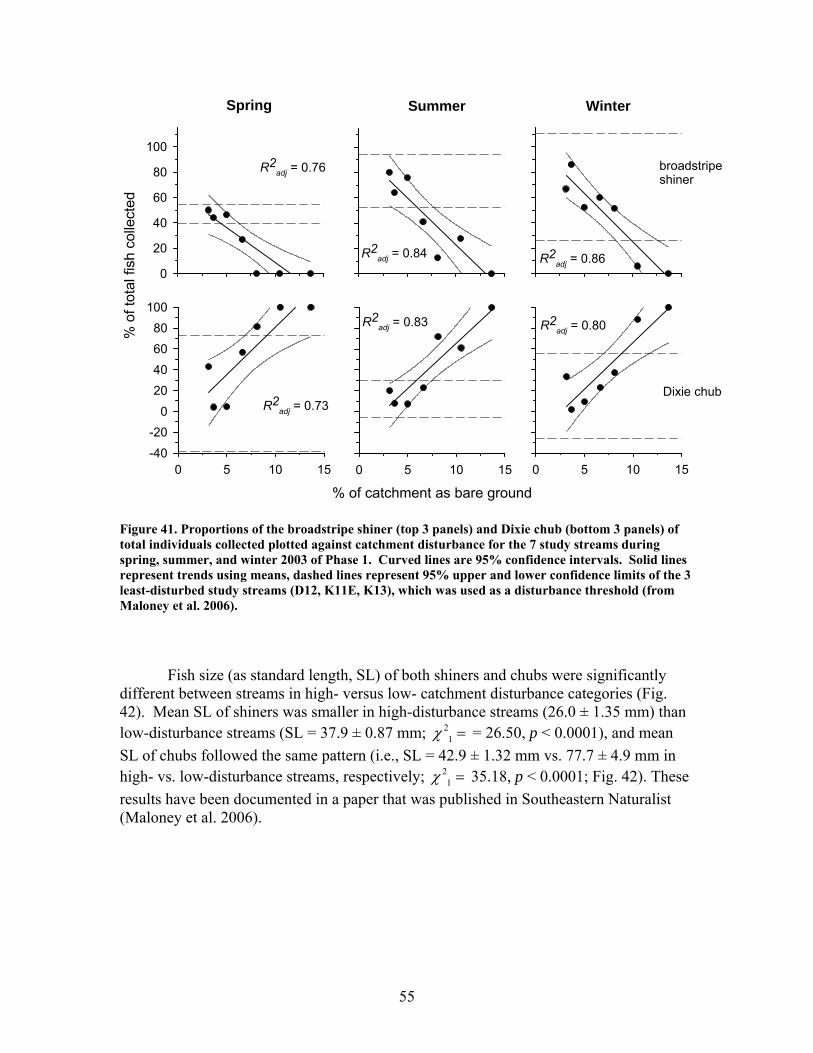
55

SummerSpring

% of catchment as bare ground0 5 10 15 0 5 10 15

0

20

40

60

80

100

0 5 10 15

% o

f tot

al fi

sh c

olle

cted

-40-20

020406080

100

broadstripeshiner

Dixie chub

Winter

R2adj = 0.76

R2adj = 0.80R2

adj = 0.83

R2adj = 0.73

R2adj = 0.86R2

adj = 0.84

Figure 41. Proportions of the broadstripe shiner (top 3 panels) and Dixie chub (bottom 3 panels) of total individuals collected plotted against catchment disturbance for the 7 study streams during spring, summer, and winter 2003 of Phase 1. Curved lines are 95% confidence intervals. Solid lines represent trends using means, dashed lines represent 95% upper and lower confidence limits of the 3 least-disturbed study streams (D12, K11E, K13), which was used as a disturbance threshold (from Maloney et al. 2006).

Fish size (as standard length, SL) of both shiners and chubs were significantly different between streams in high- versus low- catchment disturbance categories (Fig. 42). Mean SL of shiners was smaller in high-disturbance streams (26.0 ± 1.35 mm) than low-disturbance streams (SL = 37.9 ± 0.87 mm; 2

1χ = = 26.50, p < 0.0001), and mean SL of chubs followed the same pattern (i.e., SL = 42.9 ± 1.32 mm vs. 77.7 ± 4.9 mm in high- vs. low-disturbance streams, respectively; 2

1χ = 35.18, p < 0.0001; Fig. 42). These results have been documented in a paper that was published in Southeastern Naturalist (Maloney et al. 2006).

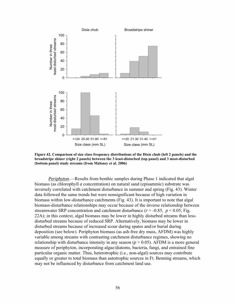
56

Size class (mm SL)<=20 21-30 31-40 >=41

Broadstripe shinerDixie chub

Num

ber i

n th

ree

leas

t-dis

turb

ed s

tream

s

0

20

40

60

80

100

Size class (mm SL)<=24 25-50 51-80 >=81

Num

ber i

n th

ree

mos

t-dis

turb

ed s

tream

s

0

20

40

60

80

100

Figure 42. Comparison of size class frequency distributions of the Dixie chub (left 2 panels) and the broadstripe shiner (right 2 panels) between the 3 least-disturbed (top panel) and 3 most-disturbed (bottom panel) study streams (from Maloney et al. 2006)

Periphyton.—Results from benthic samples during Phase 1 indicated that algal biomass (as chlorophyll a concentration) on natural sand (episammic) substrate was inversely correlated with catchment disturbance in summer and spring (Fig. 43). Winter data followed the same trends but were nonsignificant because of high variation in biomass within low-disturbance catchments (Fig. 43). It is important to note that algal biomass-disturbance relationships may occur because of the inverse relationship between streamwater SRP concentration and catchment disturbance (r = -0.85, p < 0.05; Fig. 22A); in this context, algal biomass may be lower in highly disturbed streams than less-disturbed streams because of reduced SRP. Alternatively, biomass may be lower in disturbed streams because of increased scour during spates and/or burial during deposition (see below). Periphyton biomass (as ash-free dry mass, AFDM) was highly variable among streams with contrasting catchment disturbance regimes, showing no relationship with disturbance intensity in any season (p > 0.05). AFDM is a more general measure of periphyton, incorporating algae/diatoms, bacteria, fungi, and entrained fine particular organic matter. Thus, heterotrophic (i.e., non-algal) sources may contribute equally or greater to total biomass than autotrophic sources in Ft. Benning streams, which may not be influenced by disturbance from catchment land use.

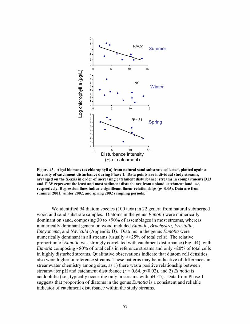
57

R2 = 0.51

0

2

4

6

8

10

0 5 10 15

012345678

0 5 10 15

R2 = 0.51

012345678

0 5 10 15

R2=.51

R2=.51

Summer

Spring

Winter

Disturbance intensity(% of catchment)

Log

chlo

roph

yll a

(μg/

L)NS

Figure 43. Algal biomass (as chlorophyll a) from natural sand substrate collected, plotted against intensity of catchment disturbance during Phase 1. Data points are individual study streams, arranged on the X-axis in order of increasing catchment disturbance: streams in compartments D13 and F1W represent the least and most sediment disturbance from upland catchment land use, respectively. Regression lines indicate significant linear relationships (p< 0.05). Data are from summer 2001, winter 2002, and spring 2002 sampling periods.

We identified 94 diatom species (100 taxa) in 22 genera from natural submerged

wood and sand substrate samples. Diatoms in the genus Eunotia were numerically dominant on sand, composing 30 to >90% of assemblages in most streams, whereas numerically dominant genera on wood included Eunotia, Brachysira, Frustulia, Encyonema, and Navicula (Appendix D). Diatoms in the genus Eunotia were numerically dominant in all streams (usually >>25% of total cells). The relative proportion of Eunotia was strongly correlated with catchment disturbance (Fig. 44), with Eunotia composing ~80% of total cells in reference streams and only ~20% of total cells in highly disturbed streams. Qualitative observations indicate that diatom cell densities also were higher in reference streams. These patterns may be indicative of differences in streamwater chemistry among sites, as 1) there was a positive relationship between streamwater pH and catchment disturbance (r = 0.64, p<0.02), and 2) Eunotia is acidophilic (i.e., typically occurring only in streams with pH <5). Data from Phase 1 suggests that proportion of diatoms in the genus Eunotia is a consistent and reliable indicator of catchment disturbance within the study streams.

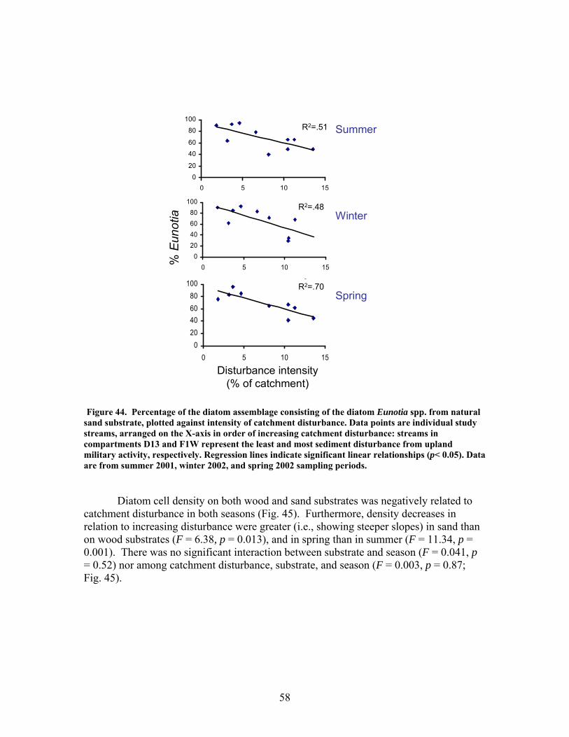
58

R2 = 0.4953

0

20

4060

80

100

0 5 10 15

R2 = 0.4842

020406080

100

0 5 10 15

R2 = 0.6969

020406080

100

0 5 10 15

R2=.48

R2=.51

R2=.70

% E

unot

ia

Summer

Winter

Spring

Disturbance intensity(% of catchment)

Figure 44. Percentage of the diatom assemblage consisting of the diatom Eunotia spp. from natural sand substrate, plotted against intensity of catchment disturbance. Data points are individual study streams, arranged on the X-axis in order of increasing catchment disturbance: streams in compartments D13 and F1W represent the least and most sediment disturbance from upland military activity, respectively. Regression lines indicate significant linear relationships (p< 0.05). Data are from summer 2001, winter 2002, and spring 2002 sampling periods.

Diatom cell density on both wood and sand substrates was negatively related to

catchment disturbance in both seasons (Fig. 45). Furthermore, density decreases in relation to increasing disturbance were greater (i.e., showing steeper slopes) in sand than on wood substrates (F = 6.38, p = 0.013), and in spring than in summer (F = 11.34, p = 0.001). There was no significant interaction between substrate and season (F = 0.041, p = 0.52) nor among catchment disturbance, substrate, and season (F = 0.003, p = 0.87; Fig. 45).

59

0 2 4 6 8 10 12 14 16

Log

diat

om d

ensi

ty (c

ells

/cm

3 )

3.0

3.5

4.0

4.5

5.0

5.5

6.0

6.5

0 2 4 6 8 10 12 14 163.0

3.5

4.0

4.5

5.0

5.5

6.0

6.5SandWood

Figure 45. Relationship between catchment disturbance intensity, as indicated by the amount of unpaved road cover or bare ground on slopes >5%) in study catchments, and diatom cell density on stream sand and wood substrates in summer (upper panel) and spring (lower panel) samples (from Miller 2006).

Disturbance intensity (% of catchment)

60

Diatom genera H’ on wood and sand were both positively related to catchment disturbance in both summer and spring (Fig. 46). Mean H’ was significantly higher on wood (1.44+0.06) than on sand (1.24+0.07) (F = 8.59, p = 0.004), and there was a marginally significant substrate–catchment disturbance interaction (F = 3.14, p = 0.079), with a greater increase in H’ with increasing disturbance on sand than on wood. Mean H’ did not differ between seasons (F = 2.60 p = 0.109), nor did season affect the relationship between H’ and catchment disturbance (F = 0.73, p = 0.39). There were no significant interactions between substrate and season (F = 0.53, p = 0.46), nor among catchment disturbance, substrate, and season (F = 1.92, p = 0.16; Fig. 46).

0 2 4 6 8 10 12 14 16

Gen

era

dive

rsity

(H')

0.0

0.5

1.0

1.5

2.0

2.5

3.0

0 2 4 6 8 10 12 14 160.0

0.5

1.0

1.5

2.0

2.5SandWood

Figure 46. Relationship between catchment disturbance intensity, as indicated by the amount of unpaved road cover or bare ground on slopes >5% in study catchments, and diatom generic-level diversity (as Shannon’s H’) on stream sand and wood substrates in summer (upper panel) and spring (lower panel) samples (from Miller 2006).

Disturbance intensity (% of catchment)

61

Bray-Curtis similarity between sand and wood assemblages in each stream in each season ranged from 28 to 68%. Sand and wood assemblages became more similar (i.e., stream substrates became more biologically homogenous) as catchment disturbance increased in spring (R2 = 0.367, p = 0.048), although similarity was unrelated to disturbance in fall/summer (R2 = 0.024, p = 0.65; Fig. 47).

Disturbance intensity

0 2 4 6 8 10 12 14 16Woo

d-sa

nd d

iato

m s

imila

rity

(1-B

ray-

Cur

tis in

dex)

0.2

0.3

0.4

0.5

0.6

0.7FallSpring

Figure 47. Relationship between catchment disturbance intensity, as indicated by the amount of unpaved road cover or bare ground on slopes >5% in each catchment, and Bray-Curtis similarities of diatom assemblages from stream sand and wood substrates, in fall/summer and spring samples (from Miller 2006).

We conducted additional analyses designed to assess if Eunotia is affected solely

by streamwater pH changes or a combination of chemical and physical conditions associated with catchment disturbance (e.g., burial by sediment in disturbed catchments). A promising periphyton metric in this regard is the ratio of tightly attached algae (i.e., cells attached to sand substrates and thus potentially more vulnerable to burial from sedimentation, such as adnate Eunotia) to unattached algae (i.e., cells loosely associated with sand substrates and thus potentially less vulnerable to sediment disturbance, such as motile Pinnularia). Separation of attached and loose cells can be accomplished by quantifying algal biomass (as chlorophyll a) on sand both before (i.e., for loose cells) and after (i.e., for more resistant attached cells) samples are sonicated. Using this measure, we observed a negative relationship between attached/ unattached algal biomass and catchment disturbance in 2 of the 3 seasons (Fig. 48). This metric may describe the impact of sedimentation independently of streamwater nutrient levels or pH, as we have

62

observed a greater proportion of motile diatoms (Pinnularia, Frustrulia, others) in the loosely attached assemblage than in tightly attached assemblages.

R2 = 0.38

0

0.2

0.4

0.6

0.8

1

0 5 10 15

0

0.2

0.4

0.6

0.8

1

0 5 10 15

R2=.38

Summer

Winter

NS

R2 = 0.50

0

0.2

0.4

0.6

0.8

1

0 5 10 15Disturbance intensity

(% of catchment)

Spring

R2=.50

Atta

ched

/una

ttach

ed A

lgal

Bio

mas

s (c

hl-a

)

Figure 48. Ratio of tightly attached (adnate) to loosely attached (flocculant) algal biomass (as chlorophyll a concentration, µg/L) from natural sand substrate, plotted against intensity of catchment disturbance. Data points are individual study streams, arranged on the X-axis in order of increasing catchment disturbance: streams in compartments D13 and F1W represent the least and most sediment disturbance from upland military activity, respectively. Regression lines indicate significant linear relationships (p< 0.05). Data are from summer 2001, winter 2002, and spring 2002 sampling periods.

Scanning Electron Microscope (SEM) observation of physiognomies on natural

streambed wood and sand substrates from indicated that diatoms on sand consisted mostly of adnate Eunotia species on the surfaces of sand particles in short chains (Fig. 49A) or as single cells (Fig. 49B). A more diverse assemblage of diatoms on wood occurred within crevices, including Frustrulia, Brachysira, and Navicula species (Fig. 49C,D). Diatoms on wood were also observed on the surface of the wood (Fig. 49D) or growing out of mucilage layers.

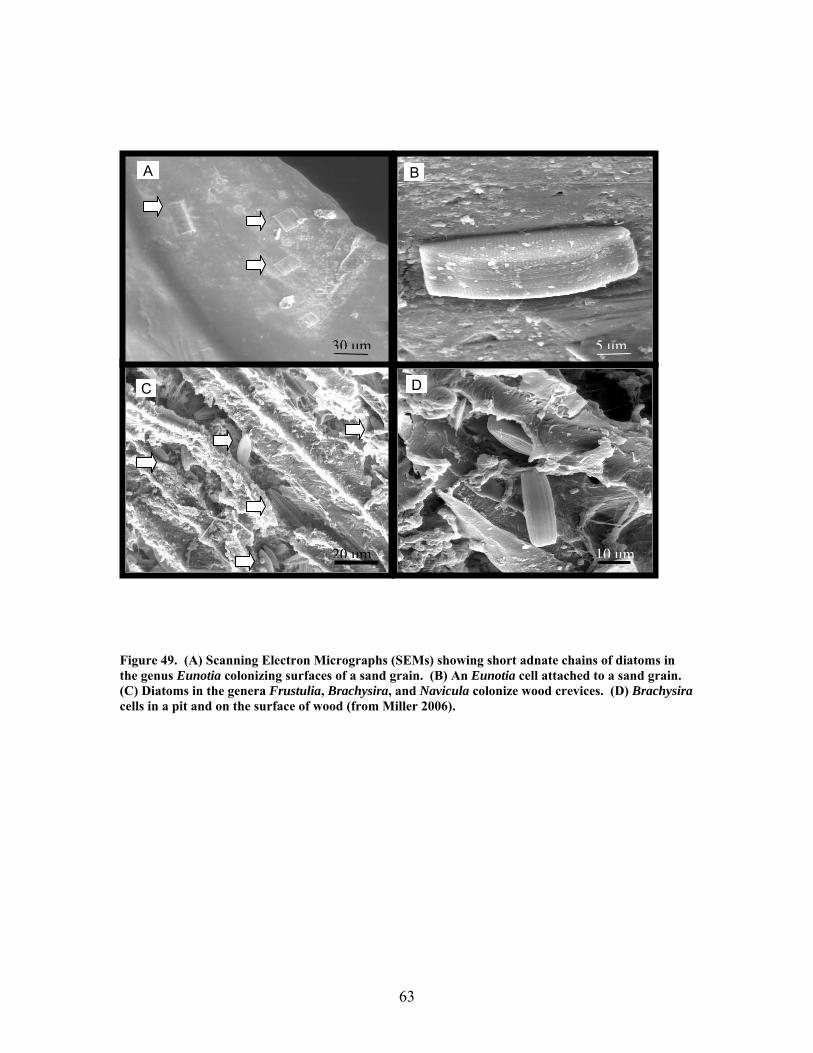
63

Figure 49. (A) Scanning Electron Micrographs (SEMs) showing short adnate chains of diatoms in the genus Eunotia colonizing surfaces of a sand grain. (B) An Eunotia cell attached to a sand grain. (C) Diatoms in the genera Frustulia, Brachysira, and Navicula colonize wood crevices. (D) Brachysira cells in a pit and on the surface of wood (from Miller 2006).

C D

A B

30 μm 5 μm

20 μm 10 μm

64

PHASE 2 - EFFECTS OF RIPARIAN AND IN-STREAM RESTORATIONS Description of Restorations Ephemeral drainage restorations. Three pilot-scale restorations of ephemeral drainages were completed. USDA-NRCS engineering aspects of the ephemeral restorations on K11E and D12 compartments were completed in mid-summer 2004. Restoration of the riparian forests near the ephemeral streams included 1) closing of point sources of sediment from roads by earth moving and rock placement; 2) sowing Coastal Bermuda grass on exposed soil and 3) planting longleaf seedlings. Catchment D12 was restored on June 2, 2004 and longleaf seedlings were planted on June 8, 2004 (see photos in Appendix C). Catchment K11E was restored on June 15, 2004 and longleaf seedlings were planted on June 23, 2004. Some locations in the D12 and K11E restorations where seedling mortality occurred as a result of planting in summer rather than the preferred periods of late fall through early spring were replanted with sweet gum in early spring 2005. The engineering aspect of the F3 restoration was completed in spring 2005 and a mixture of water oak and longleaf pine were planted. Instream restorations. We created artificial woody debris dams within 100-150 m reaches in 4 of the 8 Phase 2 streams (K11E, K20, F3, F1E) during 25-27 October 2003 by adding coarse woody debris (CWD) to these streams (see photos in Appendix C). Disturbed streams in compartments D12, D13, F1W, F4 were left unrestored to serve as controls. We used blackgum (Nyssa sylvatica) wood for K11E, F3, and F1E restorations and white oak (Quercus alba) for K20 restorations. Riparian trees used in restorations were felled and sectioned during August 2003 to allow wood dry for 2 to 3 months prior to deployment, and anchored in situ with rebar stakes. The amount of CWD added to each restored stream was measured to determine total area of wood added. Wood additions was left in place for the duration of the project, and temporal changes in stream habitat and biota between Phase 1 (before restoration) and Phase 2 (after restoration) were compared with those observed in unrestored (control) streams. Prior to instream restorations, abundance and spatial distribution of natural debris dams were quantified in each Phase 2 (after restoration) stream (K11E, K20, D12, D13, F1E, F1W, F3, F4), by measuring wood surface area, % litter cover and average current velocity within each debris dam encountered over the study reach. Our measurements indicated that debris dams increased the percent areal coverage of CWD by 3.1 % (K20) to 5.2 % (F3) resulting in total CWD coverage of 6.9 % (K20) to 12.1 % (K11E) in the restored streams (Table 1; see also Fig. 28). Prior to beginning the 2nd year of Phase 2, we observed that excessive sedimentation in some streams caused rapid burial of many debris dams, with some dams becoming almost completed buried within 6 mo (Fig. 39). Thus, in 2004 we augmented the original 2003 wood additions in 2 of the 4 restored streams (F1E, K20). Both streams had only received instream restoration in 2003, with no ephemeral channel restoration. On 9 November 2004 we added additional wood to F1E and K20 (i.e., adding white oak wood in K20 and hickory [Carya sp.] and black gum wood in F1E). After this 2nd

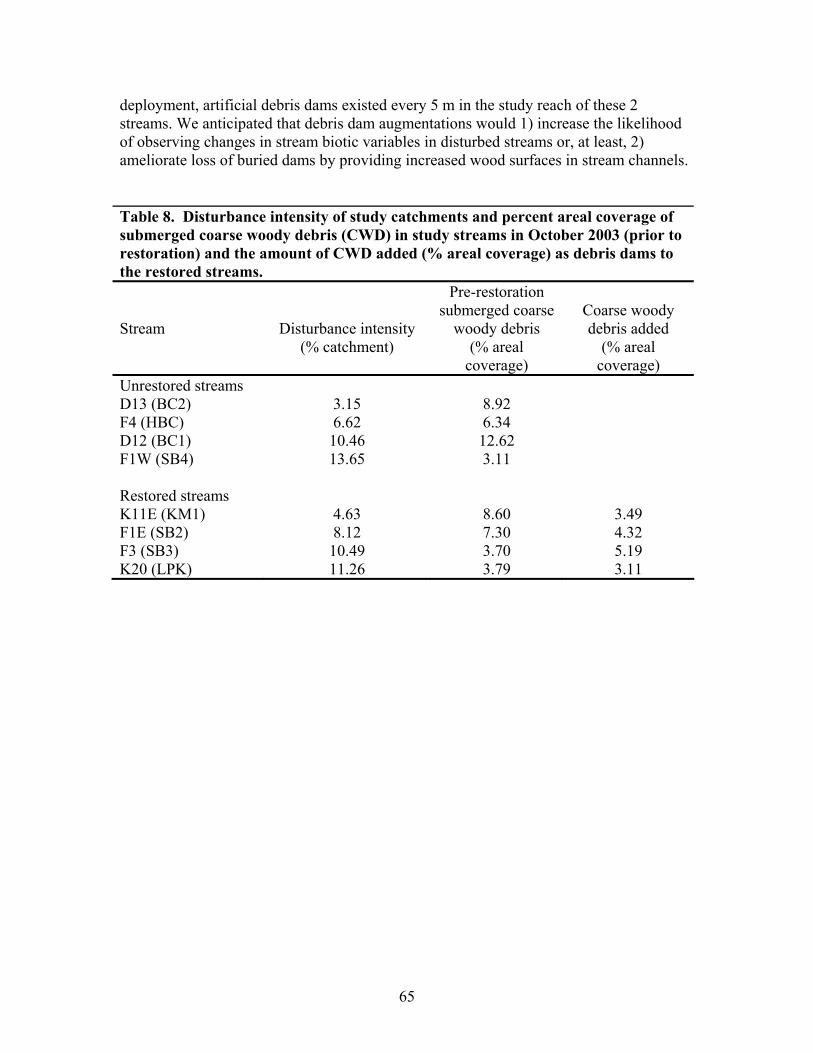
65

deployment, artificial debris dams existed every 5 m in the study reach of these 2 streams. We anticipated that debris dam augmentations would 1) increase the likelihood of observing changes in stream biotic variables in disturbed streams or, at least, 2) ameliorate loss of buried dams by providing increased wood surfaces in stream channels. Table 8. Disturbance intensity of study catchments and percent areal coverage of submerged coarse woody debris (CWD) in study streams in October 2003 (prior to restoration) and the amount of CWD added (% areal coverage) as debris dams to the restored streams. Stream

Disturbance intensity (% catchment)

Pre-restoration submerged coarse

woody debris (% areal

coverage)

Coarse woody debris added

(% areal coverage)

Unrestored streams D13 (BC2) 3.15 8.92 F4 (HBC) 6.62 6.34 D12 (BC1) 10.46 12.62 F1W (SB4) 13.65 3.11 Restored streams K11E (KM1) 4.63 8.60 3.49 F1E (SB2) 8.12 7.30 4.32 F3 (SB3) 10.49 3.70 5.19 K20 (LPK) 11.26 3.79 3.11

66

Responses to Ephemeral Drainage Restorations Technical Approach

Erosion from unpaved forest roads has led to substantial sediment accumulation in riparian forests at Ft. Benning, GA. This sedimentation has been associated with declines in productivity, nutrient cycling, and community diversity. In order to reduce sediment flow into riparian forests, three watersheds (D12, F3, and K11) underwent restoration efforts aimed at reducing erosion from upland roads. Restoration measures included re-contouring hill slopes, installing rip-rock and fabric dams along drainages, creating sediment basins, seeding grasses, and planting trees. The most significant restoration efforts were in D12, where the road was permanently closed to traffic, re-contoured, and planted with grasses and trees. Restoration efforts in D12 and K11 were completed in June and July of 2004 and, for F3, in June of 2005. The effectiveness of restoration was evaluated by comparing sedimentation, productivity, nutrient cycling, and community composition before and after restoration. Three reference watersheds (two watersheds in F4 and one in I3) were used as controls. The time period for pre-restoration in D12, K11, and reference plots was from January 2002 to June 2004, with post-restoration from July 2004 to December 2006. Pre- and post-restoration for F3 was considered from January 2002 to June 2005 and from July 2005 to December 2006, respectively.

Sedimentation rates were measured using 6-8 sediment pins in each plot.

Sediment pins were composed of a metal washer attached to a metal rod and inserted in the ground so that the washer was directly on top of the soil surface. Sediment which accumulated on top of the washer was measured monthly from December 2001 through December 2006. Aboveground net primary productivity (ANPP) was estimated based on litterfall, collected monthly from 3 0.25 m-2 litterfall traps per plot, and woody increments of trees (>5 cm DBH). Belowground net primary productivity (BNPP) was estimated by sampling fine roots every six weeks. Significant increases in live root biomass between sample periods were summed over 12 months to estimate annual belowground productivity. Total net primary productivity (NPP) was estimated by summing ANPP and BNPP. Standing crop biomass of trees, shrubs and saplings (<5 cm DBH), and roots were also monitored throughout the study period. Trees, shrubs, and understory vegetation were sampled annually to determine community diversity, richness, and evenness. Nutrient cycling was evaluated based on plant nutrients, N mineralization, microbial biomass, and decomposition rates. Significant differences in means between the two time periods were determined using one-way analysis of variance (ANOVA) tests. Site Characteristics

The treatment (restored) plots (F3, D12, and K11) are similar in terms of topographic position but vary in regard to moisture regime. Plot K11 is categorized as xeric in terms of soil and vegetation composition while D12 and F3 are mesic.

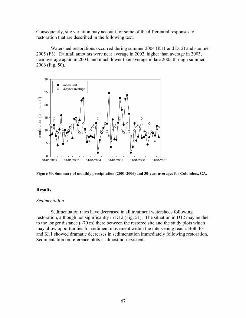
67

Consequently, site variation may account for some of the differential responses to restoration that are described in the following text.

Watershed restorations occurred during summer 2004 (K11 and D12) and summer

2005 (F3). Rainfall amounts were near average in 2002, higher than average in 2003, near average again in 2004, and much lower than average in late 2005 through summer 2006 (Fig. 50).

01/01/2002 01/01/2003 01/01/2004 01/01/2005 01/01/2006 01/01/2007

prec

ipita

tion

(cm

mon

th-1

)

0

5

10

15

20

25

30

measured30 year average

Figure 50. Summary of monthly precipitation (2001-2006) and 30-year averages for Columbus, GA.

Results Sedimentation Sedimentation rates have decreased in all treatment watersheds following restoration, although not significantly in D12 (Fig. 51). The situation in D12 may be due to the longer distance (~70 m) there between the restored site and the study plots which may allow opportunities for sediment movement within the intervening reach. Both F3 and K11 showed dramatic decreases in sedimentation immediately following restoration. Sedimentation on reference plots is almost non-existent.

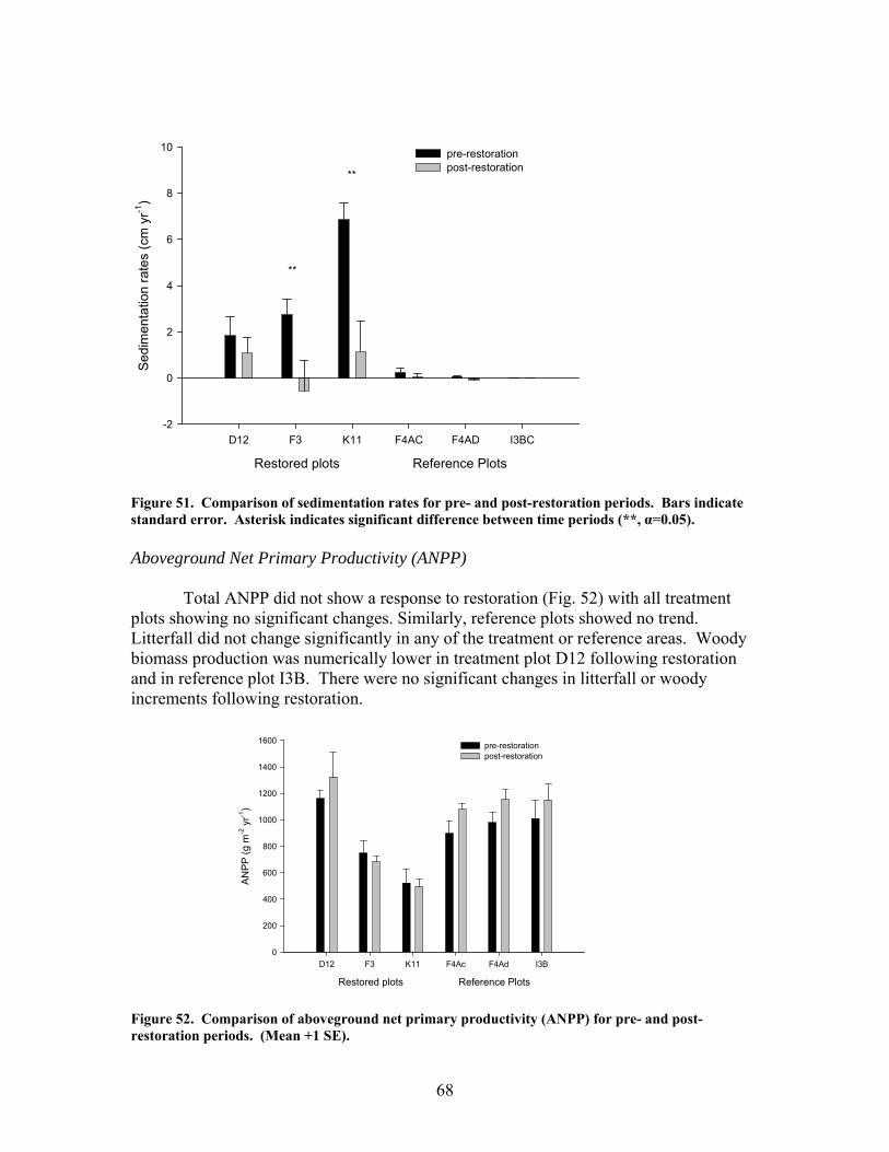
68

Restored plots Reference Plots

D12 F3 K11 F4AC F4AD I3BC

Sed

imen

tatio

n ra

tes

(cm

yr-1

)

-2

0

2

4

6

8

10 pre-restorationpost-restoration

**

**

Figure 51. Comparison of sedimentation rates for pre- and post-restoration periods. Bars indicate standard error. Asterisk indicates significant difference between time periods (**, α=0.05). Aboveground Net Primary Productivity (ANPP) Total ANPP did not show a response to restoration (Fig. 52) with all treatment plots showing no significant changes. Similarly, reference plots showed no trend. Litterfall did not change significantly in any of the treatment or reference areas. Woody biomass production was numerically lower in treatment plot D12 following restoration and in reference plot I3B. There were no significant changes in litterfall or woody increments following restoration.

Restored plots Reference Plots

D12 F3 K11 F4Ac F4Ad I3B

AN

PP

(g m

-2 y

r-1)

0

200

400

600

800

1000

1200

1400

1600 pre-restorationpost-restoration

Figure 52. Comparison of aboveground net primary productivity (ANPP) for pre- and post-restoration periods. (Mean +1 SE).

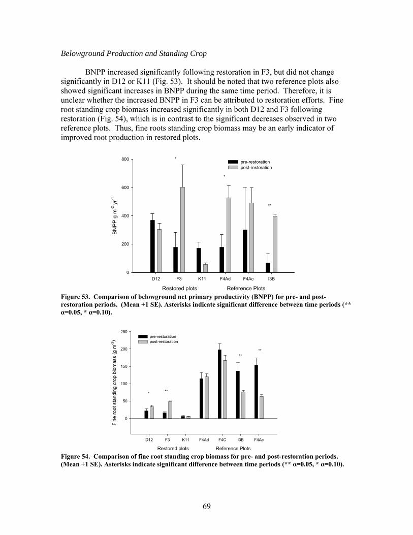
69

Belowground Production and Standing Crop

BNPP increased significantly following restoration in F3, but did not change significantly in D12 or K11 (Fig. 53). It should be noted that two reference plots also showed significant increases in BNPP during the same time period. Therefore, it is unclear whether the increased BNPP in F3 can be attributed to restoration efforts. Fine root standing crop biomass increased significantly in both D12 and F3 following restoration (Fig. 54), which is in contrast to the significant decreases observed in two reference plots. Thus, fine roots standing crop biomass may be an early indicator of improved root production in restored plots.

Restored plots Reference Plots

D12 F3 K11 F4Ad F4Ac I3B

BNPP

g m

-2 y

r-1

0

200

400

600

800 pre-restorationpost-restoration

*

*

**

Figure 53. Comparison of belowground net primary productivity (BNPP) for pre- and post-restoration periods. (Mean +1 SE). Asterisks indicate significant difference between time periods (** α=0.05, * α=0.10).

Restored plots Reference Plots

D12 F3 K11 F4Ad F4C I3B F4Ac

Fine

root

sta

ndin

g cr

op b

iom

ass

(g m

-2)

0

50

100

150

200

250pre-restorationpost-restoration

* **

****

Figure 54. Comparison of fine root standing crop biomass for pre- and post-restoration periods. (Mean +1 SE). Asterisks indicate significant difference between time periods (** α=0.05, * α=0.10).

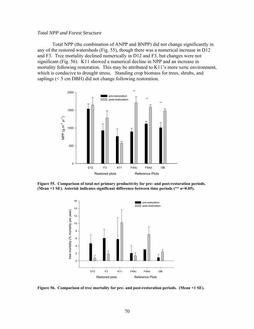
70

Total NPP and Forest Structure

Total NPP (the combination of ANPP and BNPP) did not change significantly in any of the restored watersheds (Fig. 55), though there was a numerical increase in D12 and F3. Tree mortality declined numerically in D12 and F3, but changes were not significant (Fig. 56). K11 showed a numerical decline in NPP and an increase in mortality following restoration. This may be attributed to K11’s more xeric environment, which is conducive to drought stress. Standing crop biomass for trees, shrubs, and saplings (< 5 cm DBH) did not change following restoration.

Restored plots Reference Plots

D12 F3 K11 F4Ac F4Ad I3B

NPP

(g m

-2 y

r-1)

0

500

1000

1500

2000pre-restorationpost-restoration

**

****

Figure 55. Comparison of total net primary productivity for pre- and post-restoration periods. (Mean +1 SE). Asterisk indicates significant difference between time periods (** α=0.05).

Restored plots Reference Plots

D12 F3 K11 F4Ac F4Ad I3B

tree

mor

talit

y (%

mor

talit

y pe

r yea

r)

0

2

4

6

8

10

12

14

16 pre-restorationpost-restoration

Figure 56. Comparison of tree mortality for pre- and post-restoration periods. (Mean +1 SE).

71

Understory Vegetation Composition No significant changes occurred on treatment plots D12 or F3 in terms of understory species (<1 m) composition following restoration. The lack of response is likely due to the low understory biomass on these plots which may stem from low light levels near the forest floor. This is in contrast with K11 where light in the understory and understory vegetation are abundant. The K11 understory showed significant increases in grasses, non-weedy species, and perennials following restoration (Fig. 57). Although data for native species suggested an increase at K11, those results were not significant. Bare ground decreased numerically in D12 and K11 following restoration, but the declines were not significant (Fig. 58). F3 was restored a year later than the others and it is uncertain whether a similar trend may occur there as well. No significant changes were found in tree or shrub community diversity, evenness, or richness.

K11

grasses nonweedy perennial native

rela

tive

impo

rtanc

e va

lue

0

2

4

6

8 pre-restorationpost-restoration

** * *

Figure 57. Comparison of relative importance values of each species group found in K11 for pre- and post-restoration periods. (Mean +1 SE). Asterisk indicates significant differences between time periods (** α=0.05, * α=0.10).

Restored plots Reference Plots

D12 F3 K11 F4A F4C

Perc

enta

ge o

f bar

e gr

ound

0

10

20

30

40

50

60 pre-restorationpost-restoration

Figure 58. Comparison of bare ground for pre- and post-restoration periods. (Mean +1 SE).

72

Nutrients in Vegetation

No significant changes were found in nutrient concentrations in litterfall samples post-restoration. N:P ratios in litterfall declined in all areas suggesting exacerbated N deficiency, a condition that may have been driven by drier conditions and reduced N mineralization during late 2005 and much of 2006. There was no indication that the decline in N availability was linked with restoration activities. Fine root samples in F3 exhibited a significant increase in C concentrations following restoration (Fig. 59), while fine roots in K11 indicated a significant increase in N (Fig. 60).

Restored plots Reference Plots

D12A F3D K11d F4Ac F4Ad I3Bc

Car

bon

in fi

ne ro

ots

(0.1

-1.0

mm

dia

met

er) m

g kg

-1

0

1e+5

2e+5

3e+5

4e+5

5e+5

6e+5 pre-restorationpost-restoration

** *** *

Figure 59. Comparison of C concentrations in live fine roots (0.1-1.0 mm diameter) for pre- and post-restoration periods. (Mean +1 SE). Asterisk indicates significant differences between time periods (** α=0.05, * α=0.10).

Restored plots Reference Plots

D12A F3D K11d F4Ac F4Ad I3BcNitr

ogen

in fi

ne ro

ots

(0.1

-1.0

mm

dia

met

er) m

g kg

-1)

0

2000

4000

6000

8000

10000

12000

14000

16000pre-restorationpost-restoration

*

**

Figure 60. Comparison of N concentrations in live fine roots (0.1-1.0 mm diameter) for pre- and post-restoration periods. (Mean +1 SE). Asterisk indicates significant differences between time periods (** α=0.05, * α=0.10).

73

Microbial Biomass C & N and Nitrogen Mineralization

As was the case before restoration, microbial biomass C and N were much lower on treatment compared to reference plots for the post-restoration period. However, there were no significant differences between pre- vs. post-restoration periods on individual treatment plots for microbial C. K11 was significantly higher in microbial N in 2003 compared to later years. Reference plot microbial biomass C and N declined significantly on F4Ad compared to the pre-restoration levels there, a condition that perhaps reflects the drier conditions during the latter period (Fig. 61).

Mineralization rates were generally similar across all plots during the post-

restoration phase. There were significant declines in F3 and in one of the reference plots (Fig. 62). Temporal patterns indicate that rates declined dramatically after fall, 2005 (i.e. the onset of a dry period), which may be more strongly evident in plots with higher pre-restoration mineralization rates (F3 and I3B).

Restored plots Reference Plots

D12 F3 K11 F4Ac F4Ad I3B

mic

robi

al C

(μg

g-1)

0

200

400

600

800pre-restorationpost-restoration

**

Figure 61. Comparison of microbial C for pre- and post-restoration periods. (Mean +1 SE). Asterisk indicates significant difference between time periods (** α=0.05).

74

Restored plots Reference Plots

D12 F3 K11 F4Ac F4Ad I3B

net N

min

eral

ized

(g h

a-1 d

-1)

0

500

1000

1500

2000

2500

pre-restorationpost-restoration

*

*

Figure 62. Comparison of N mineralization rates for pre- and post-restoration periods. (Mean +1 SE). Asterisk indicates significant difference between time periods (* α=0.10).

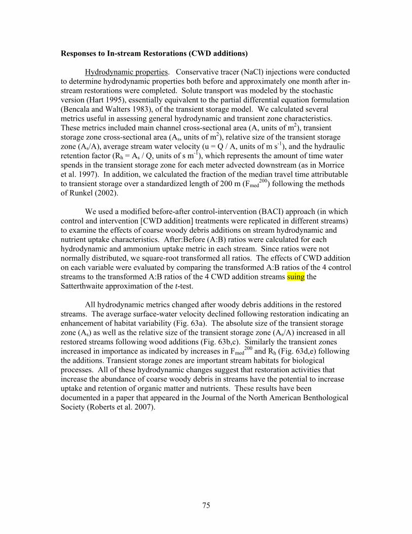
75

Responses to In-stream Restorations (CWD additions)

Hydrodynamic properties. Conservative tracer (NaCl) injections were conducted to determine hydrodynamic properties both before and approximately one month after in-stream restorations were completed. Solute transport was modeled by the stochastic version (Hart 1995), essentially equivalent to the partial differential equation formulation (Bencala and Walters 1983), of the transient storage model. We calculated several metrics useful in assessing general hydrodynamic and transient zone characteristics. These metrics included main channel cross-sectional area (A, units of m2), transient storage zone cross-sectional area (As, units of m2), relative size of the transient storage zone (As/A), average stream water velocity (u = Q / A, units of m s-1), and the hydraulic retention factor (Rh = As / Q, units of s m-1), which represents the amount of time water spends in the transient storage zone for each meter advected downstream (as in Morrice et al. 1997). In addition, we calculated the fraction of the median travel time attributable to transient storage over a standardized length of 200 m (Fmed

200) following the methods of Runkel (2002). We used a modified before-after control-intervention (BACI) approach (in which control and intervention [CWD addition] treatments were replicated in different streams) to examine the effects of coarse woody debris additions on stream hydrodynamic and nutrient uptake characteristics. After:Before (A:B) ratios were calculated for each hydrodynamic and ammonium uptake metric in each stream. Since ratios were not normally distributed, we square-root transformed all ratios. The effects of CWD addition on each variable were evaluated by comparing the transformed A:B ratios of the 4 control streams to the transformed A:B ratios of the 4 CWD addition streams suing the Satterthwaite approximation of the t-test. All hydrodynamic metrics changed after woody debris additions in the restored streams. The average surface-water velocity declined following restoration indicating an enhancement of habitat variability (Fig. 63a). The absolute size of the transient storage zone (As) as well as the relative size of the transient storage zone (As/A) increased in all restored streams following wood additions (Fig. 63b,c). Similarly the transient zones increased in importance as indicated by increases in Fmed

200 and Rh (Fig. 63d,e) following the additions. Transient storage zones are important stream habitats for biological processes. All of these hydrodynamic changes suggest that restoration activities that increase the abundance of coarse woody debris in streams have the potential to increase uptake and retention of organic matter and nutrients. These results have been documented in a paper that appeared in the Journal of the North American Benthological Society (Roberts et al. 2007).

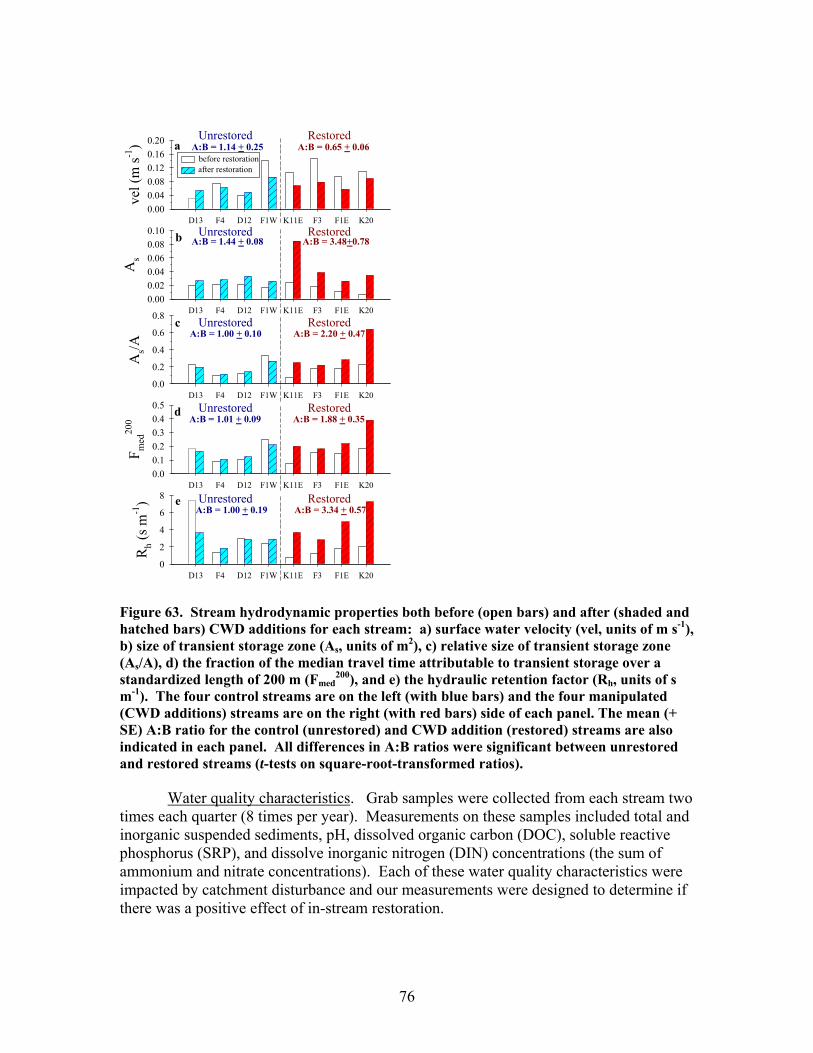
76

D13 F4 D12 F1W K11E F3 F1E K20

As

0.000.020.040.060.080.10

D13 F4 D12 F1W K11E F3 F1E K20

F med

200

0.00.10.20.30.40.5

D13 F4 D12 F1W K11E F3 F1E K20

vel (

m s-1

)

0.000.040.080.120.160.20

A:B = 1.14 + 0.25 A:B = 0.65 + 0.06Unrestored Restored

b

a

D13 F4 D12 F1W K11E F3 F1E K20

As/A

0.0

0.2

0.4

0.6

0.8

D13 F4 D12 F1W K11E F3 F1E K20

Rh (

s m-1

)

0

2

4

6

8

c

d

e

Unrestored Restored

Unrestored Restored

Unrestored Restored

Unrestored Restored

before restorationafter restoration

A:B = 1.44 + 0.08 A:B = 3.48+0.78

A:B = 1.00 + 0.10 A:B = 2.20 + 0.47

A:B = 1.01 + 0.09 A:B = 1.88 + 0.35

A:B = 1.00 + 0.19 A:B = 3.34 + 0.57

Figure 63. Stream hydrodynamic properties both before (open bars) and after (shaded and hatched bars) CWD additions for each stream: a) surface water velocity (vel, units of m s-1), b) size of transient storage zone (As, units of m2), c) relative size of transient storage zone (As/A), d) the fraction of the median travel time attributable to transient storage over a standardized length of 200 m (Fmed

200), and e) the hydraulic retention factor (Rh, units of s m-1). The four control streams are on the left (with blue bars) and the four manipulated (CWD additions) streams are on the right (with red bars) side of each panel. The mean (+ SE) A:B ratio for the control (unrestored) and CWD addition (restored) streams are also indicated in each panel. All differences in A:B ratios were significant between unrestored and restored streams (t-tests on square-root-transformed ratios). Water quality characteristics. Grab samples were collected from each stream two times each quarter (8 times per year). Measurements on these samples included total and inorganic suspended sediments, pH, dissolved organic carbon (DOC), soluble reactive phosphorus (SRP), and dissolve inorganic nitrogen (DIN) concentrations (the sum of ammonium and nitrate concentrations). Each of these water quality characteristics were impacted by catchment disturbance and our measurements were designed to determine if there was a positive effect of in-stream restoration.

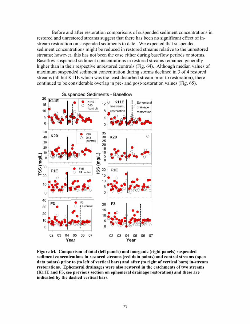
77

Before and after restoration comparisons of suspended sediment concentrations in restored and unrestored streams suggest that there has been no significant effect of in-stream restoration on suspended sediments to date. We expected that suspended sediment concentrations might be reduced in restored streams relative to the unrestored streams; however, this has not been the case either during baseflow periods or storms. Baseflow suspended sediment concentrations in restored streams remained generally higher than in their respective unrestored controls (Fig. 64). Although median values of maximum suspended sediment concentration during storms declined in 3 of 4 restored streams (all but K11E which was the least disturbed stream prior to restoration), there continued to be considerable overlap in pre- and post-restoration values (Fig. 65).

K11E

TSS

(mg/

L)

0

5

10

15

20K11ED13 (control)

K11EIS

S (m

g/L)

0

4

8

12

K20

05

101520253035

Suspended Sediments - Baseflow

F1E

0

10

20

30 F1EF4 control F1E

05

101520

F3

Year02 03 04 05 06 07

0

10

20

30

40F3F4 control

F3

Year02 03 04 05 06 07

05

101520

In-streamrestoration

Ephemeraldrainagerestoration

K20

01020304050

K20D13(control)

Figure 64. Comparison of total (left panels) and inorganic (right panels) suspended sediment concentrations in restored streams (red data points) and control streams (open data points) prior to (to left of vertical bars) and after (to right of vertical bars) in-stream restorations. Ephemeral drainages were also restored in the catchments of two streams (K11E and F3, see previous section on ephemeral drainage restoration) and these are indicated by the dashed vertical bars.

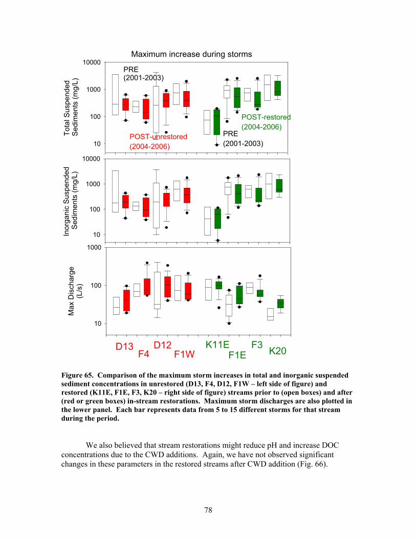
78

Maximum increase during stormsTo

tal S

uspe

nded

S

edim

ents

(mg/

L)

10

100

1000

10000In

orga

nic

Susp

ende

d S

edim

ents

(mg/

L)

10

100

1000

10000

Max

Dis

char

ge(L

/s)

10

100

1000

D13F4

D12F1W

K11EF1E

F3 K20

PRE(2001-2003)

POST-unrestored(2004-2006)

PRE (2001-2003)

POST-restored(2004-2006)

Figure 65. Comparison of the maximum storm increases in total and inorganic suspended sediment concentrations in unrestored (D13, F4, D12, F1W – left side of figure) and restored (K11E, F1E, F3, K20 – right side of figure) streams prior to (open boxes) and after (red or green boxes) in-stream restorations. Maximum storm discharges are also plotted in the lower panel. Each bar represents data from 5 to 15 different storms for that stream during the period. We also believed that stream restorations might reduce pH and increase DOC concentrations due to the CWD additions. Again, we have not observed significant changes in these parameters in the restored streams after CWD addition (Fig. 66).

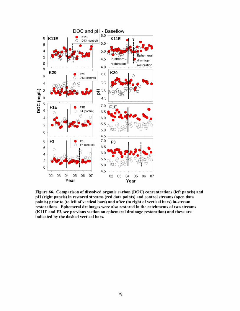
79

K11ED

OC

(mg/

L)

0

2

4

6

8 K11ED13 (control) K11E

pH

4.0

4.5

5.0

5.5

6.0

K20

X Data

0

2

4

6

8K20D13 (control)

K20

4.5

5.0

5.5

6.0

DOC and pH - Baseflow

F1E

X Data

0

2

4

6

8F1EF4 (control)

F1E

X Data

4.5

5.0

5.5

6.0

6.5

7.0

F3

Year02 03 04 05 06 07

0

2

4

6

8 F3F4 (control)

F3

Year02 03 04 05 06 07

4.5

5.0

5.5

6.0

6.5

7.0

In-streamrestoration

Ephemeraldrainagerestoration

Figure 66. Comparison of dissolved organic carbon (DOC) concentrations (left panels) and pH (right panels) in restored streams (red data points) and control streams (open data points) prior to (to left of vertical bars) and after (to right of vertical bars) in-stream restorations. Ephemeral drainages were also restored in the catchments of two streams (K11E and F3, see previous section on ephemeral drainage restoration) and these are indicated by the dashed vertical bars.

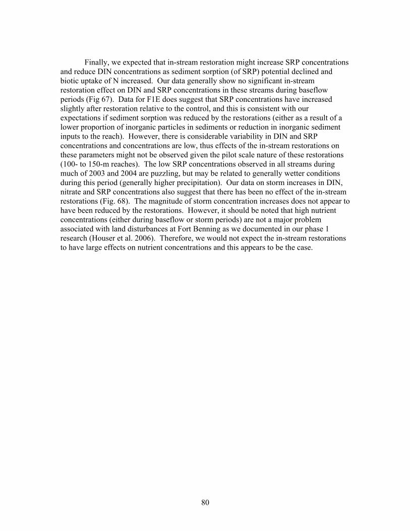
80

Finally, we expected that in-stream restoration might increase SRP concentrations and reduce DIN concentrations as sediment sorption (of SRP) potential declined and biotic uptake of N increased. Our data generally show no significant in-stream restoration effect on DIN and SRP concentrations in these streams during baseflow periods (Fig 67). Data for F1E does suggest that SRP concentrations have increased slightly after restoration relative to the control, and this is consistent with our expectations if sediment sorption was reduced by the restorations (either as a result of a lower proportion of inorganic particles in sediments or reduction in inorganic sediment inputs to the reach). However, there is considerable variability in DIN and SRP concentrations and concentrations are low, thus effects of the in-stream restorations on these parameters might not be observed given the pilot scale nature of these restorations (100- to 150-m reaches). The low SRP concentrations observed in all streams during much of 2003 and 2004 are puzzling, but may be related to generally wetter conditions during this period (generally higher precipitation). Our data on storm increases in DIN, nitrate and SRP concentrations also suggest that there has been no effect of the in-stream restorations (Fig. 68). The magnitude of storm concentration increases does not appear to have been reduced by the restorations. However, it should be noted that high nutrient concentrations (either during baseflow or storm periods) are not a major problem associated with land disturbances at Fort Benning as we documented in our phase 1 research (Houser et al. 2006). Therefore, we would not expect the in-stream restorations to have large effects on nutrient concentrations and this appears to be the case.

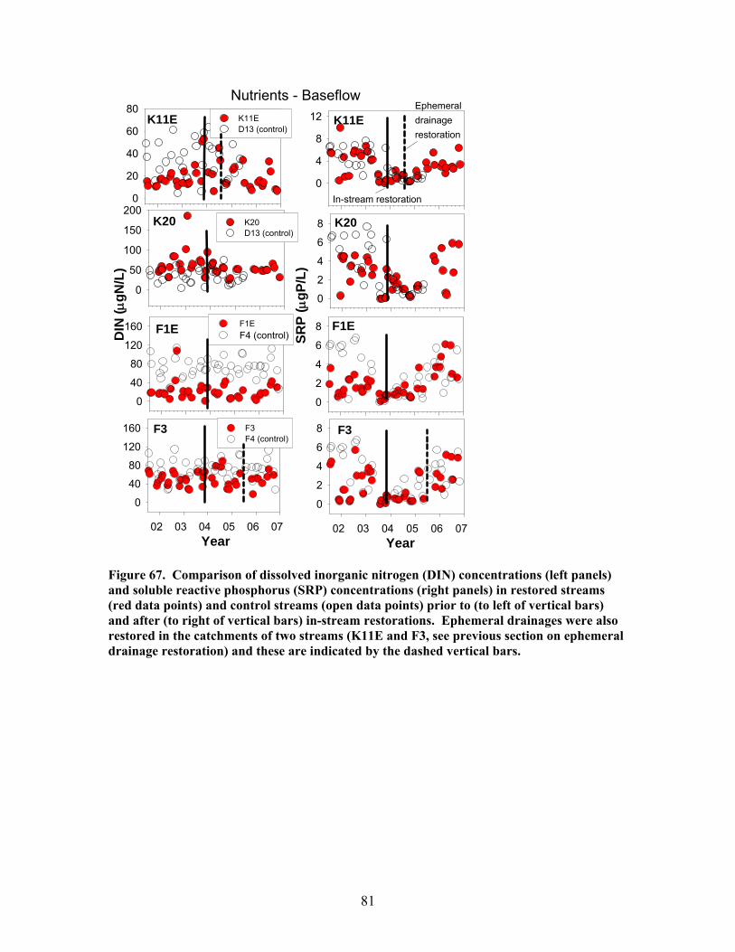
81

K11ED

IN (μ

gN/L

)

0

20

40

60

80K11ED13 (control)

K11E

SRP

( μgP

/L)

0

4

8

12

K20

0

50

100

150

200K20D13 (control)

K20

0

2

4

6

8

Nutrients - Baseflow

F1E

0

40

80

120

160 F1EF4 (control)

F1E

0

2

4

6

8

F3

Year02 03 04 05 06 07

0

40

80

120

160 F3F4 (control)

F3

Year02 03 04 05 06 07

0

2

4

6

8

In-stream restoration

Ephemeraldrainagerestoration

Figure 67. Comparison of dissolved inorganic nitrogen (DIN) concentrations (left panels) and soluble reactive phosphorus (SRP) concentrations (right panels) in restored streams (red data points) and control streams (open data points) prior to (to left of vertical bars) and after (to right of vertical bars) in-stream restorations. Ephemeral drainages were also restored in the catchments of two streams (K11E and F3, see previous section on ephemeral drainage restoration) and these are indicated by the dashed vertical bars.

82

Maximum increase during storms D

isso

lved

inor

gani

c N

(μ

gN/L

)

1

10

100

1000

Nitr

ate

(μgN

/L)

1

10

100

1000

Sol

uble

reac

tive

P(μ

gP/L

)

0

5

10

15

D13F4

D12F1W

K11EF1E

F3 K20

PRE(2001-2003)

POST-unrestored(2004-2006)

POST-restored(2004-2006)

Figure 68. Comparison of the maximum storm increases in dissolved inorganic N, nitrate, and soluble reactive phosphorus in unrestored (D13, F4, D12, F1W – left side of figure) and restored (K11E, F1E, F3, K20 – right side of figure) streams prior to (open boxes) and after (red or green boxes) in-stream restorations. Each bar represents data from 5 to 15 different storms for that stream during the period. Nutrient uptake rates. Short-term (1-2 hour) ammonium addition (NH4) experiments were conducted at the same time as the conservative tracer injections just prior to and about 3 weeks after stream restorations to assess the effects of restoration on nutrient uptake rates. Ammonium uptake rates were determined from the ammonium addition experiments and expressed as a fractional uptake rate from water per unit distance (k, units of m-1), an uptake velocity (Vf, units of m s-1), and a mass removal rate from water per unit area (U, units of mg NH4-N m-2 s-1).

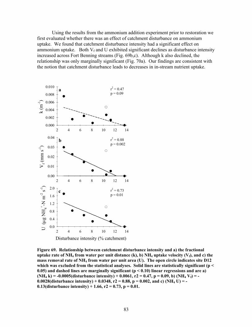
83

Using the results from the ammonium addition experiment prior to restoration we first evaluated whether there was an effect of catchment disturbance on ammonium uptake. We found that catchment disturbance intensity had a significant effect on ammonium uptake. Both Vf and U exhibited significant declines as disturbance intensity increased across Fort Benning streams (Fig. 69b,c). Although k also declined, the relationship was only marginally significant (Fig. 70a). Our findings are consistent with the notion that catchment disturbance leads to decreases in in-stream nutrient uptake.

2 4 6 8 10 12 14U (μg

NH

4+ -N m

-2 s-1

)

0.0

0.4

0.8

1.2

1.6

2.0

2 4 6 8 10 12 14

Vf (

mm

s-1)

0.00

0.01

0.02

0.03

0.04

2 4 6 8 10 12 14

k (m

-1)

0.000

0.002

0.004

0.006

0.008

0.010

Disturbance intensity (% catchment)

r2 = 0.88p = 0.002

r2 = 0.73p = 0.01

a

b

c

r2 = 0.47p = 0.09

Figure 69. Relationship between catchment disturbance intensity and a) the fractional uptake rate of NH4 from water per unit distance (k), b) NH4 uptake velocity (Vf), and c) the mass removal rate of NH4 from water per unit area (U). The open circle indicates site D12 which was excluded from the statistical analyses. Solid lines are statistically significant (p < 0.05) and dashed lines are marginally significant (p < 0.10) linear regressions and are a) (NH4 k) = -0.0005(disturbance intensity) + 0.0061, r2 = 0.47, p = 0.09, b) (NH4 Vf) = -0.0028(disturbance intensity) + 0.0348, r2 = 0.88, p = 0.002, and c) (NH4 U) = -0.13(disturbance intensity) + 1.66, r2 = 0.73, p = 0.01.

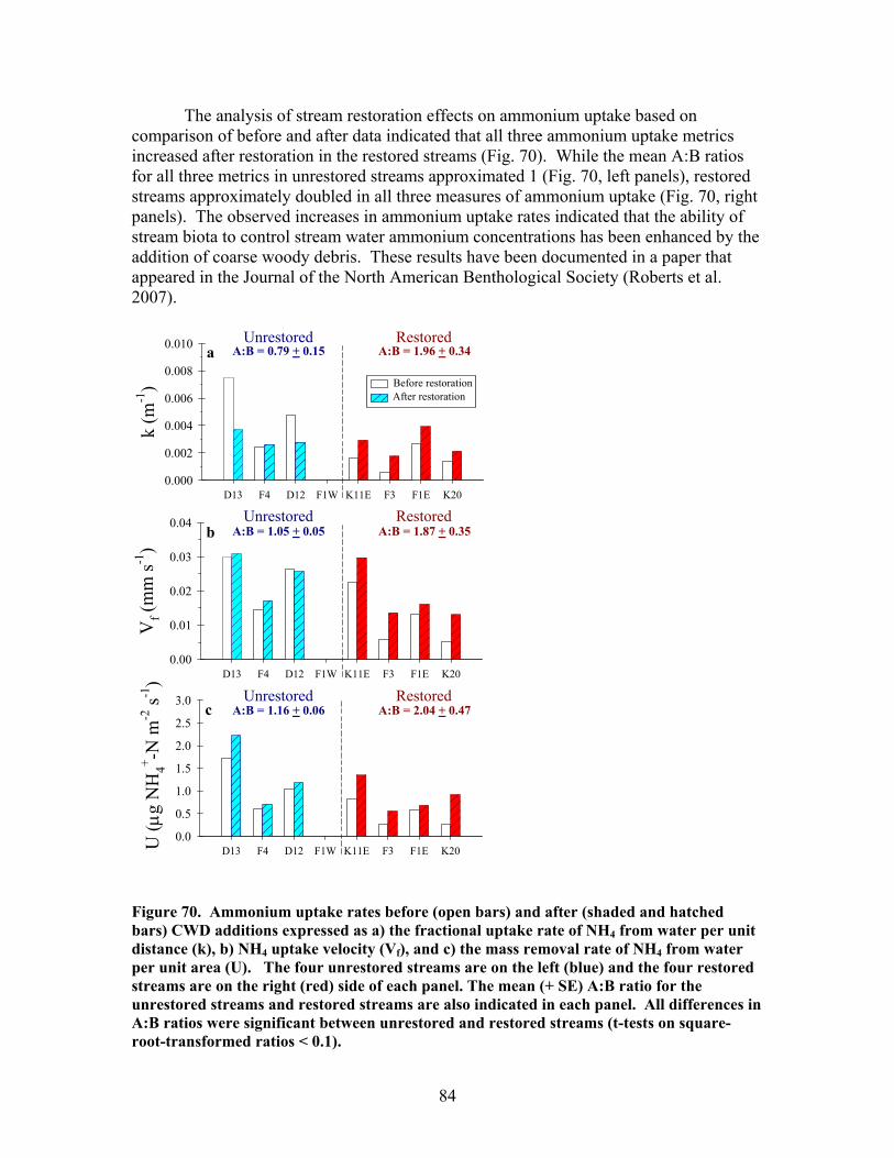
84

The analysis of stream restoration effects on ammonium uptake based on comparison of before and after data indicated that all three ammonium uptake metrics increased after restoration in the restored streams (Fig. 70). While the mean A:B ratios for all three metrics in unrestored streams approximated 1 (Fig. 70, left panels), restored streams approximately doubled in all three measures of ammonium uptake (Fig. 70, right panels). The observed increases in ammonium uptake rates indicated that the ability of stream biota to control stream water ammonium concentrations has been enhanced by the addition of coarse woody debris. These results have been documented in a paper that appeared in the Journal of the North American Benthological Society (Roberts et al. 2007).

Unrestored Restored

D13 F4 D12 F1W K11E F3 F1E K20

Vf (

mm

s-1)

0.00

0.01

0.02

0.03

0.04

D13 F4 D12 F1W K11E F3 F1E K20U ( μ

g N

H4+ -N

m-2

s-1)

0.0

0.5

1.0

1.5

2.0

2.5

3.0

a

b

c

A:B = 0.79 + 0.15 A:B = 1.96 + 0.34

D13 F4 D12 F1W K11E F3 F1E K20

k (m

-1)

0.000

0.002

0.004

0.006

0.008

0.010

Unrestored Restored

Unrestored Restored

Before restorationAfter restoration

A:B = 1.05 + 0.05 A:B = 1.87 + 0.35

A:B = 1.16 + 0.06 A:B = 2.04 + 0.47

Figure 70. Ammonium uptake rates before (open bars) and after (shaded and hatched bars) CWD additions expressed as a) the fractional uptake rate of NH4 from water per unit distance (k), b) NH4 uptake velocity (Vf), and c) the mass removal rate of NH4 from water per unit area (U). The four unrestored streams are on the left (blue) and the four restored streams are on the right (red) side of each panel. The mean (+ SE) A:B ratio for the unrestored streams and restored streams are also indicated in each panel. All differences in A:B ratios were significant between unrestored and restored streams (t-tests on square-root-transformed ratios < 0.1).

85

Stream metabolism rates. To study the effects of the stream restorations on stream ecosystem metabolism, we continued measuring metabolism in each of four seasons following the restorations in the eight streams included in Phase 2 of the project. We deployed a YSI dissolved oxygen sonde in each stream for a 2 to 3 week period each season to determine gross primary production (GPP) and ecosystem respiration (ER) rates using the one-station diel oxygen change method (Bott 1996, Houser et al. 2005). We conducted short-term salt and propane injections in each stream at the time of dissolved oxygen sonde deployment to determine water discharge rate, average water velocity, and air-water dissolved gas exchange rate—all of which are required for calculating GPP and ER rates. We used a modified before-after control-intervention (BACI) approach (in which both control and intervention [CWD addition] locations were replicated) to examine the effects of coarse woody debris additions on stream ecosystem metabolism rates. As a result of the strong seasonal differences in metabolism rates observed in phase 1 of this project, we are evaluating the effects of the woody additions on a seasonal basis. We calculated seasonal mean GPP and ER rates in each stream during each year of the study. We have calculated seasonal mean rates for the before restoration period (2001-2003) and compared these rates to the seasonal mean rates for each year after restoration (2004-2006) in order to examine both the effectiveness of the CWD additions as well as the duration over which any positive effects may persist.

GPP rates were low throughout the entire study. During the first year post-CWD addition (2004), GPP exhibited little change in the restored streams (Fig. 71). During autumn 2004, winter 2005, and spring 2005, GPP increased in 3 of the 4 restored streams (Fig. 71). This is consistent with our observations of substantial algal growth on the coarse woody debris added to these streams. After:Before (A:B) manipulation ratios of GPP rates in restored streams (Fig. 72, shaded bars) were significantly higher than in unrestored streams (Fig. 72, open bars) in these seasons (p< 0.1 in autumn 2004 and p < 0.05 in winter and spring 2005). No effects of restoration on GPP were observed after spring 2005 (Figs. 71 and 72). This is not surprising given the low rates of GPP found outside of the winter-spring, open canopy period.

In contrast to GPP, respiration rates exhibited a wide range of values throughout

the study. All four restored streams exhibited higher respiration rates for all seasons in 2004 and 2005 than during the period prior to CWD additions (Fig. 73). A:B respiration ratios were higher in restored streams than in unrestored streams in all seasons of 2004 and 2005 (Fig. 74). These differences between A:B respiration ratios for unrestored and restored streams were significant in all seasons except spring 2004 (p< 0.1 in winter and summer 2004, p< 0.05 from autumn 2004 through summer 2005, and p< 0.01 in autumn 2005; Fig. 74). During the first two years after CWD was added to the restored streams, respiration generally increased during all seasons (Fig. 73) with the largest increases being observed in the two streams with the most highly disturbed catchments (F1E and

86

K20). We found that pre-manipulation disturbance intensity had a significant effect on magnitude of response to CWD additions (Fig. 75).

In 2006 (3rd year after CWD was added), neither GPP nor ER rates were

significantly higher in any of the restored streams during any season than in the before restoration (2001-2003) period (Fig. 71 and 73, hatched bars and Figs. 72 and 74). The observed reduction in metabolism rates between the 2nd and 3rd year post-restoration is likely a result of substantial burial of the course woody debris experimentally added to the study streams (between 32 and 78% of the CWD added to the study streams was buried after 2 years, see Fig. 78). Our findings suggest that coarse woody debris additions resulted in an initial increase in biotic activity in Fort Benning streams, but in order for this increase to persist for multiple years the sediment load from upland disturbances must be reduced.

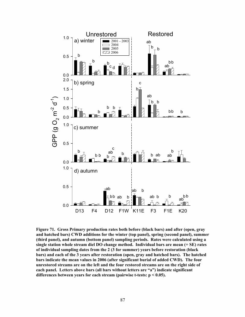
87

Figure 71. Gross Primary production rates both before (black bars) and after (open, gray and hatched bars) CWD additions for the winter (top panel), spring (second panel), summer (third panel), and autumn (bottom panel) sampling periods. Rates were calculated using a single station whole stream diel DO change method. Individual bars are mean (+ SE) rates of individual sampling dates from the 2 (3 for summer) years before restoration (black bars) and each of the 3 years after restoration (open, gray and hatched bars). The hatched bars indicate the mean values in 2006 (after significant burial of added CWD). The four unrestored streams are on the left and the four restored streams are on the right side of each panel. Letters above bars (all bars without letters are “a”) indicate significant differences between years for each stream (pairwise t-tests: p < 0.05).

a) winter

0.0

0.5

1.0

b) spring

0.0

0.5

1.0

1.5

2.0

c) summer

GP

P (g

O2 m

-2 d

-1)

0.0

0.5

1.0

d) autumn

D13 F4 D12 F1W K11E F3 F1E K200.0

0.5

1.0

Unrestored Restored2001 - 2003200420052006

b

c

ab

d

b b

b b abbb

bb b

bc

abb b

bbb

bb b

abb

cb b ab ab

b

bb

ab

ab bab b

ab b b b bab

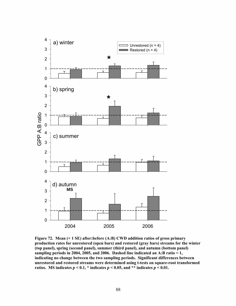
88

Figure 72. Mean (+ 1 SE) after:before (A:B) CWD addition ratios of gross primary production rates for unrestored (open bars) and restored (gray bars) streams for the winter (top panel), spring (second panel), summer (third panel), and autumn (bottom panel) sampling periods in 2004, 2005, and 2006. Dashed line indicated an A:B ratio = 1, indicating no change between the two sampling periods. Significant differences between unrestored and restored streams were determined using t-tests on square-root transformed ratios. MS indicates p < 0.1, * indicates p < 0.05, and ** indicates p < 0.01.

a) winter

0

1

2

3

4Unrestored (n = 4) Restored (n = 4)

b) spring

0

1

2

3

4

c) summer

GP

P A

:B ra

tio

0

1

2

3

4

d) autumn

2004 2005 20060

1

2

3

4

*

*

MS

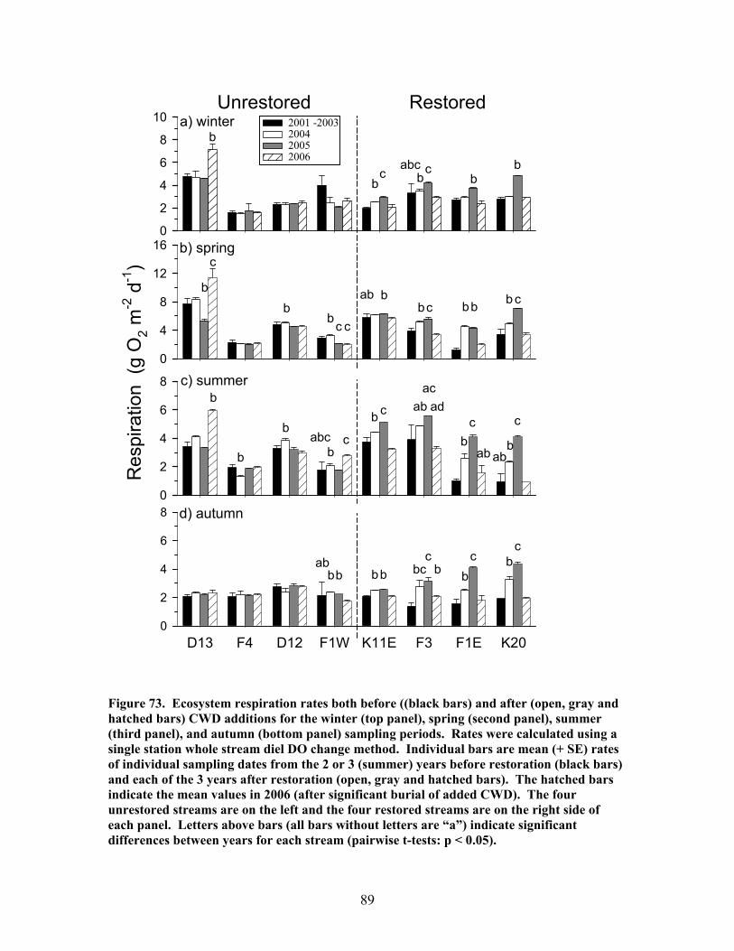
89

Figure 73. Ecosystem respiration rates both before ((black bars) and after (open, gray and hatched bars) CWD additions for the winter (top panel), spring (second panel), summer (third panel), and autumn (bottom panel) sampling periods. Rates were calculated using a single station whole stream diel DO change method. Individual bars are mean (+ SE) rates of individual sampling dates from the 2 or 3 (summer) years before restoration (black bars) and each of the 3 years after restoration (open, gray and hatched bars). The hatched bars indicate the mean values in 2006 (after significant burial of added CWD). The four unrestored streams are on the left and the four restored streams are on the right side of each panel. Letters above bars (all bars without letters are “a”) indicate significant differences between years for each stream (pairwise t-tests: p < 0.05).

b) spring

0

4

8

12

16

c) summer

Res

pira

tion

(g O

2 m-2

d-1

)

0

2

4

6

8

d) autumn

D13 F4 D12 F1W K11E F3 F1E K200

2

4

6

8

a) winter

0

2

4

6

8

10Unrestored Restored

2001 -2003200420052006

b

bc

abcb b

b

b cbbbcab b

bc cb

b

c

b

b

bb c

b

abac

ad

bc

ab b

abbb bb bc

cb b

c bc

abc

c

c

abc

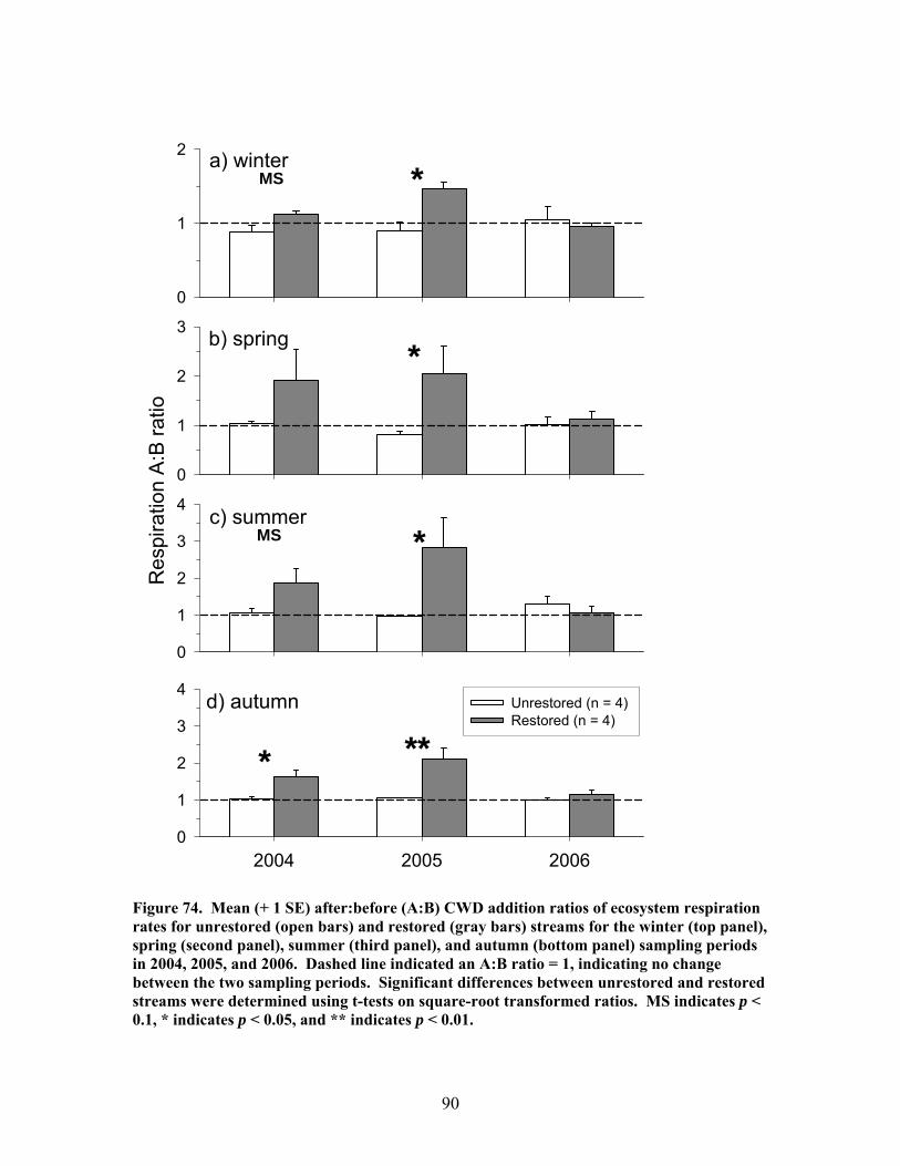
90

Figure 74. Mean (+ 1 SE) after:before (A:B) CWD addition ratios of ecosystem respiration rates for unrestored (open bars) and restored (gray bars) streams for the winter (top panel), spring (second panel), summer (third panel), and autumn (bottom panel) sampling periods in 2004, 2005, and 2006. Dashed line indicated an A:B ratio = 1, indicating no change between the two sampling periods. Significant differences between unrestored and restored streams were determined using t-tests on square-root transformed ratios. MS indicates p < 0.1, * indicates p < 0.05, and ** indicates p < 0.01.

a) winter

0

1

2

b) spring

0

1

2

3

c) summer

Res

pira

tion

A:B

ratio

0

1

2

3

4

d) autumn

2004 2005 20060

1

2

3

4Unrestored (n = 4) Restored (n = 4)

*

*

***

*

MS

MS

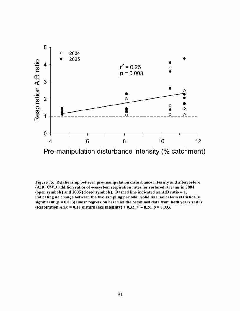
91

Figure 75. Relationship between pre-manipulation disturbance intensity and after:before (A:B) CWD addition ratios of ecosystem respiration rates for restored streams in 2004 (open symbols) and 2005 (closed symbols). Dashed line indicated an A:B ratio = 1, indicating no change between the two sampling periods. Solid line indicates a statistically significant (p = 0.003) linear regression based on the combined data from both years and is (Respiration A:B) = 0.18(disturbance intensity) + 0.32, r2 – 0.26, p = 0.003.

Pre-manipulation disturbance intensity (% catchment)4 6 8 10 12

Res

pira

tion

A:B

ratio

0

1

2

3

4

520042005

r2 = 0.26p = 0.003

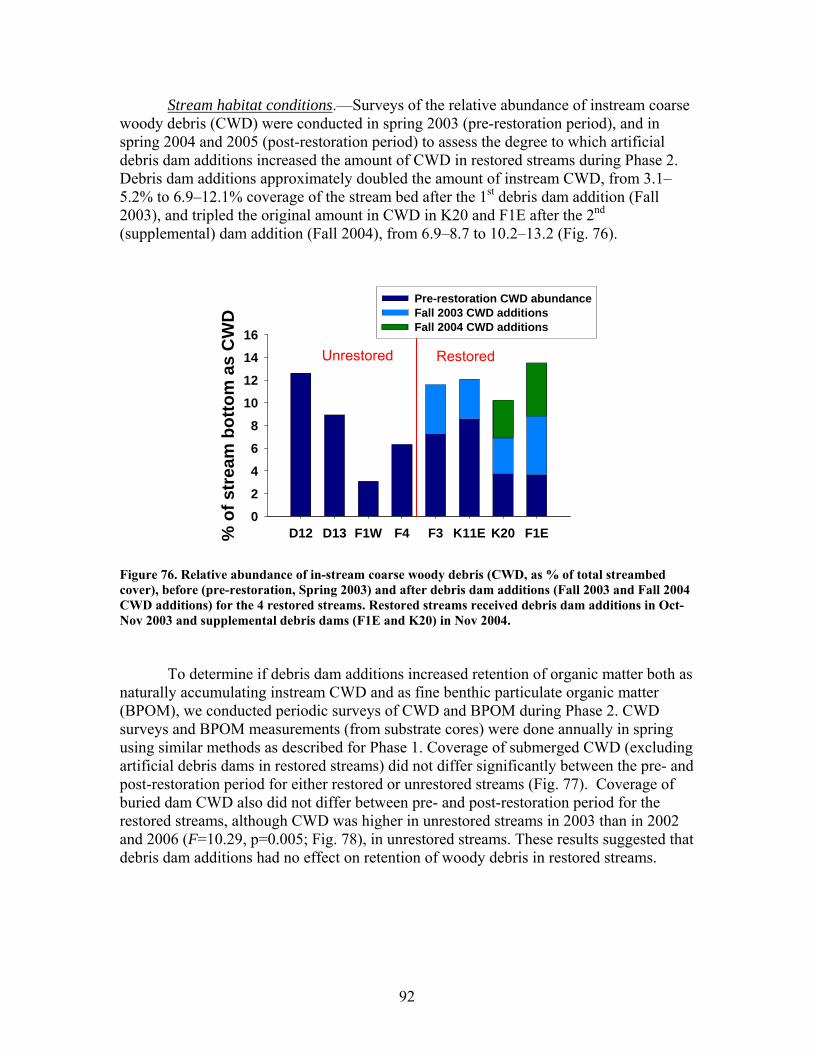
92

Stream habitat conditions.—Surveys of the relative abundance of instream coarse woody debris (CWD) were conducted in spring 2003 (pre-restoration period), and in spring 2004 and 2005 (post-restoration period) to assess the degree to which artificial debris dam additions increased the amount of CWD in restored streams during Phase 2. Debris dam additions approximately doubled the amount of instream CWD, from 3.1–5.2% to 6.9–12.1% coverage of the stream bed after the 1st debris dam addition (Fall 2003), and tripled the original amount in CWD in K20 and F1E after the 2nd (supplemental) dam addition (Fall 2004), from 6.9–8.7 to 10.2–13.2 (Fig. 76). Figure 76. Relative abundance of in-stream coarse woody debris (CWD, as % of total streambed cover), before (pre-restoration, Spring 2003) and after debris dam additions (Fall 2003 and Fall 2004 CWD additions) for the 4 restored streams. Restored streams received debris dam additions in Oct-Nov 2003 and supplemental debris dams (F1E and K20) in Nov 2004.

To determine if debris dam additions increased retention of organic matter both as naturally accumulating instream CWD and as fine benthic particulate organic matter (BPOM), we conducted periodic surveys of CWD and BPOM during Phase 2. CWD surveys and BPOM measurements (from substrate cores) were done annually in spring using similar methods as described for Phase 1. Coverage of submerged CWD (excluding artificial debris dams in restored streams) did not differ significantly between the pre- and post-restoration period for either restored or unrestored streams (Fig. 77). Coverage of buried dam CWD also did not differ between pre- and post-restoration period for the restored streams, although CWD was higher in unrestored streams in 2003 than in 2002 and 2006 (F=10.29, p=0.005; Fig. 78), in unrestored streams. These results suggested that debris dam additions had no effect on retention of woody debris in restored streams.

D12 D13 F1W F4 F3 K11E K20 F1E% o

f str

eam

bot

tom

as

CW

D

0

2

4

6

8

10

12

14

16

Pre-restoration CWD abundanceFall 2003 CWD additionsFall 2004 CWD additions

Unrestored Restored

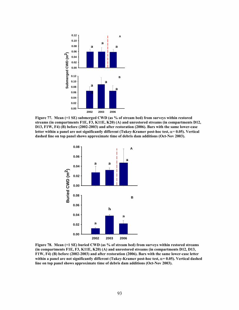
93

Subm

erge

d C

WD

(m2 )

0.00

0.02

0.04

0.06

0.08

0.10

0.12

2002 2003 20060.00

0.02

0.04

0.06

0.08

0.10

0.12

A

B

Figure 77. Mean (+1 SE) submerged CWD (as % of stream bed) from surveys within restored streams (in compartments F1E, F3, K11E, K20) (A) and unrestored streams (in compartments D12, D13, F1W, F4) (B) before (2002-2003) and after restoration (2006). Bars with the same lower-case letter within a panel are not significantly different (Tukey-Kramer post-hoc test, α= 0.05). Vertical dashed line on top panel shows approximate time of debris dam additions (Oct-Nov 2003).

Bur

ied

CW

D (m

2 )

0.00

0.02

0.04

0.06

0.08

2002 2003 20060.00

0.02

0.04

0.06

0.08

A

B

Figure 78. Mean (+1 SE) buried CWD (as % of stream bed) from surveys within restored streams (in compartments F1E, F3, K11E, K20) (A) and unrestored streams (in compartments D12, D13, F1W, F4) (B) before (2002-2003) and after restoration (2006). Bars with the same lower-case letter within a panel are not significantly different (Tukey-Kramer post-hoc test, α= 0.05). Vertical dashed line on top panel shows approximate time of debris dam additions (Oct-Nov 2003).

aa

a

aa

a

ba

a

a aa

a

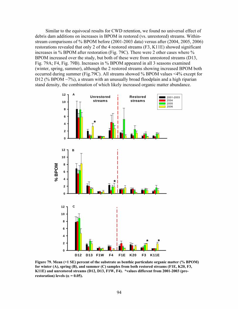
94

Similar to the equivocal results for CWD retention, we found no universal effect of debris dam additions on increases in BPOM in restored (vs. unrestored) streams. Within-stream comparisons of % BPOM before (2001-2003 data) versus after (2004, 2005, 2006) restorations revealed that only 2 of the 4 restored streams (F3, K11E) showed significant increases in % BPOM after restoration (Fig. 79C). There were 2 other cases where % BPOM increased over the study, but both of these were from unrestored streams (D13, Fig. 79A; F4, Fig. 79B). Increases in % BPOM appeared in all 3 seasons examined (winter, spring, summer), although the 2 restored streams showing increased BPOM both occurred during summer (Fig.79C). All streams showed % BPOM values <4% except for D12 (% BPOM ~7%), a stream with an unusually broad floodplain and a high riparian stand density, the combination of which likely increased organic matter abundance.

% B

POM

0

2

4

6

8

10

12

0

2

4

6

8

10

122001-2003200420052006

Unrestoredstreams

Restoredstreams

D12 D13 F1W F4 F1E K20 F3 K11E0

2

4

6

8

10

12

*

* *

*

A

C

B

Figure 79. Mean (+1 SE) percent of the substrate as benthic particulate organic matter (% BPOM) for winter (A), spring (B), and summer (C) samples from both restored streams (F1E, K20, F3, K11E) and unrestored streams (D12, D13, F1W, F4). *values different from 2001-2003 (pre-restoration) levels (α = 0.05).

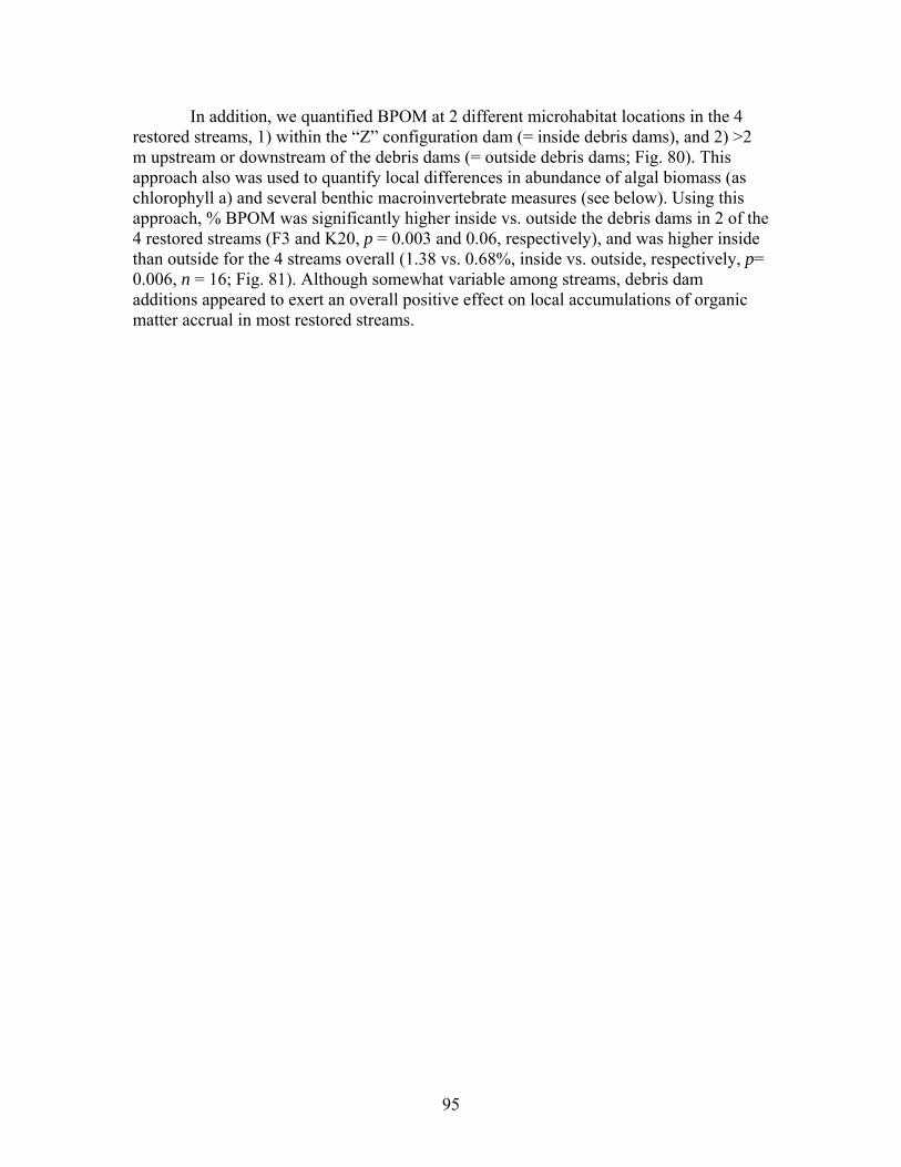
95

In addition, we quantified BPOM at 2 different microhabitat locations in the 4 restored streams, 1) within the “Z” configuration dam (= inside debris dams), and 2) >2 m upstream or downstream of the debris dams (= outside debris dams; Fig. 80). This approach also was used to quantify local differences in abundance of algal biomass (as chlorophyll a) and several benthic macroinvertebrate measures (see below). Using this approach, % BPOM was significantly higher inside vs. outside the debris dams in 2 of the 4 restored streams (F3 and K20, p = 0.003 and 0.06, respectively), and was higher inside than outside for the 4 streams overall (1.38 vs. 0.68%, inside vs. outside, respectively, p= 0.006, n = 16; Fig. 81). Although somewhat variable among streams, debris dam additions appeared to exert an overall positive effect on local accumulations of organic matter accrual in most restored streams.

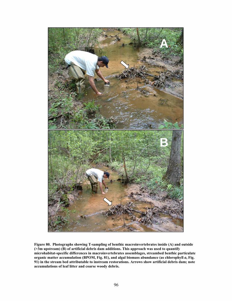
96

Figure 80. Photographs showing T-sampling of benthic macroinvertebrates inside (A) and outside (>3m upstream) (B) of artificial debris dam additions. This approach was used to quantify microhabitat-specific differences in macroinvertebrates assemblages, streambed benthic particulate organic matter accumulation (BPOM, Fig. 81), and algal biomass abundance (as chlorophyll a, Fig. 91) in the stream bed attributable to instream restorations. Arrows show artificial debris dam; note accumulations of leaf litter and coarse woody debris.

A

B

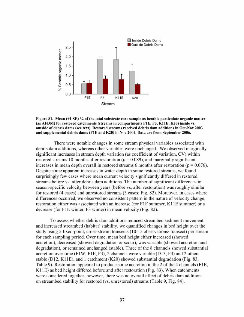
97

F3 K20F1E K11E

% B

enth

ic o

rgan

ic m

atte

r

0.0

0.5

1.0

1.5

2.0

2.5

Inside Debris DamsOutside Debris Dams

Stream

Figure 81. Mean (+1 SE) % of the total substrate core sample as benthic particulate organic matter (as AFDM) for restored catchments (streams in compartments F1E, F3, K11E, K20) inside vs. outside of debris dams (see text). Restored streams received debris dam additions in Oct-Nov 2003 and supplemental debris dams (F1E and K20) in Nov 2004. Data are from September 2006.

There were notable changes in some stream physical variables associated with

debris dam additions, whereas other variables were unchanged. We observed marginally significant increases in stream depth variation (as coefficient of variation, CV) within restored streams 10 months after restoration (p = 0.089), and marginally significant increases in mean depth overall in restored streams 6 months after restoration (p = 0.076). Despite some apparent increases in water depth in some restored streams, we found surprisingly few cases where mean current velocity significantly differed in restored streams before vs. after debris dam additions. The number of significant differences in season-specific velocity between years (before vs. after restoration) was roughly similar for restored (4 cases) and unrestored streams (3 cases; Fig. 82). Moreover, in cases where differences occurred, we observed no consistent pattern in the nature of velocity change; restoration either was associated with an increase (for F1E summer, K11E summer) or a decrease (for F1E winter, F3 winter) in mean velocity (Fig. 82).

To assess whether debris dam additions reduced streambed sediment movement

and increased streambed (habitat) stability, we quantified changes in bed height over the study using 5 fixed-point, cross-stream transects (10-15 observations/ transect) per stream for each sampling period. Over time, mean bed height either increased (showed accretion), decreased (showed degradation or scour), was variable (showed accretion and degradation), or remained unchanged (stable). Three of the 8 channels showed substantial accretion over time (F1W, F1E, F3), 2 channels were variable (D13, F4) and 2 others stable (D12, K11E), and 1 catchment (K20) showed substantial degradation (Fig. 83, Table 9). Restoration appeared to produce some accretion in the 2 of the 4 channels (F1E, K11E) as bed height differed before and after restoration (Fig. 83). When catchments were considered together, however, there was no overall effect of debris dam additions on streambed stability for restored (vs. unrestored) streams (Table 9, Fig. 84).

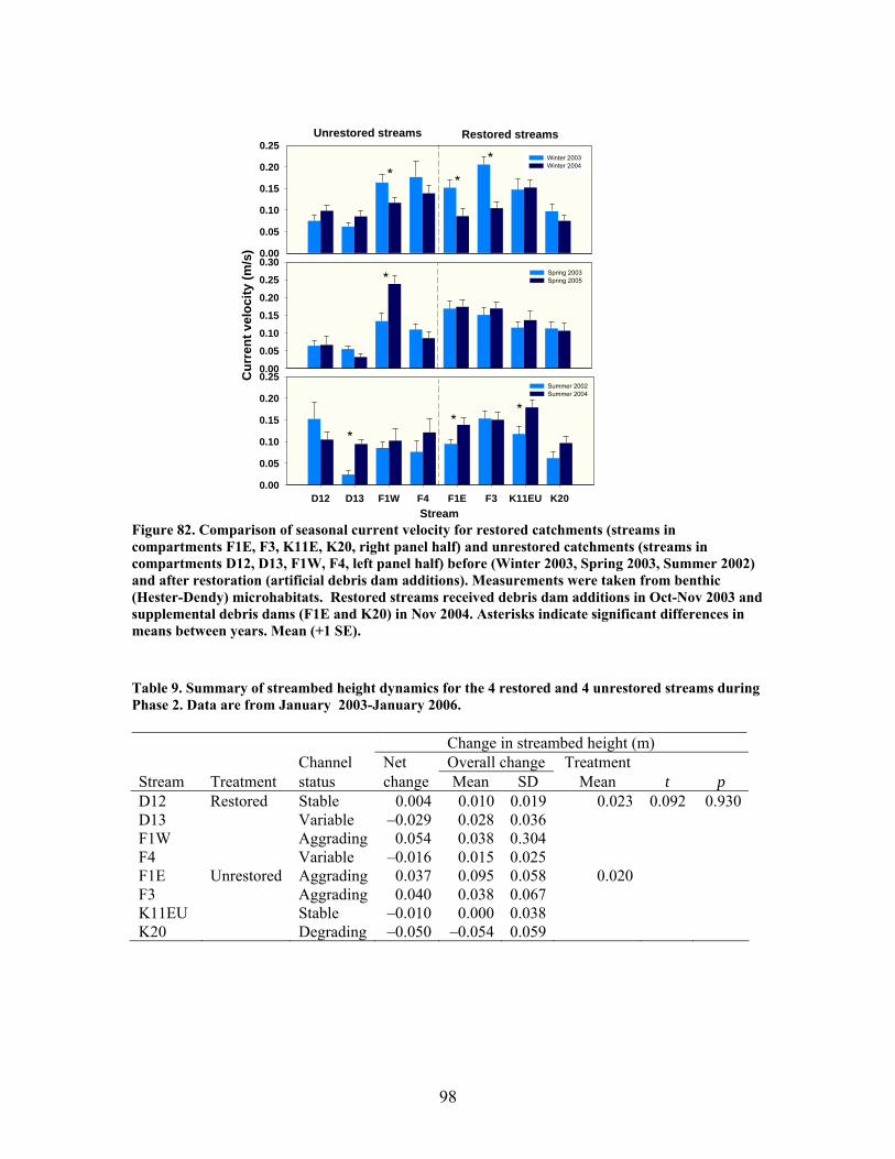
98

0.00

0.05

0.10

0.15

0.20

0.25Winter 2003 Winter 2004

Cur

rent

vel

ocity

(m/s

)

0.00

0.05

0.10

0.15

0.20

0.25

0.30Spring 2003Spring 2005

D12 D13 F1W F4 F1E F3 K11EU K200.00

0.05

0.10

0.15

0.20

0.25Summer 2002Summer 2004

Unrestored streams Restored streams

* **

*

**

*

Stream Figure 82. Comparison of seasonal current velocity for restored catchments (streams in compartments F1E, F3, K11E, K20, right panel half) and unrestored catchments (streams in compartments D12, D13, F1W, F4, left panel half) before (Winter 2003, Spring 2003, Summer 2002) and after restoration (artificial debris dam additions). Measurements were taken from benthic (Hester-Dendy) microhabitats. Restored streams received debris dam additions in Oct-Nov 2003 and supplemental debris dams (F1E and K20) in Nov 2004. Asterisks indicate significant differences in means between years. Mean (+1 SE).

Table 9. Summary of streambed height dynamics for the 4 restored and 4 unrestored streams during Phase 2. Data are from January 2003-January 2006. ______________________________________________________________________ Change in streambed height (m) Channel Net Overall change Treatment Stream Treatment status change Mean SD Mean t p D12 Restored Stable 0.004 0.010 0.019 0.023 0.092 0.930 D13 Variable –0.029 0.028 0.036 F1W Aggrading 0.054 0.038 0.304 F4 Variable –0.016 0.015 0.025 F1E Unrestored Aggrading 0.037 0.095 0.058 0.020 F3 Aggrading 0.040 0.038 0.067 K11EU Stable –0.010 0.000 0.038 K20 Degrading –0.050 –0.054 0.059

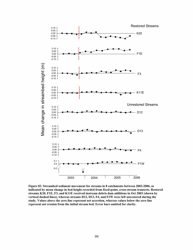
99

K20-0.10-0.050.000.050.10

F1E

-0.10-0.050.000.050.10

F3-0.10-0.050.000.050.10

K11E

Mea

n ch

ange

in s

tream

bed

heig

ht (m

)

-0.10-0.050.000.050.10

D12-0.10-0.050.000.050.10

D13

-0.10-0.050.000.050.10

F4-0.10-0.050.000.050.10

F1W-0.2

0.00.1

Restored Streams

Unrestored Streams

2003 2004 2005 2006

Figure 83. Streambed sediment movement for streams in 8 catchments between 2003-2006, as indicated by mean change in bed height recorded from fixed-point, cross-stream transects. Restored streams K20, F1E, F3, and K11E received instream debris dam additions in Oct 2003 (shown by vertical dashed lines), whereas streams D12, D13, F4, and F1W were left unrestored during the study. Values above the zero line represent net accretion, whereas values below the zero line represent net erosion from the initial stream bed. Error bars omitted for clarity.

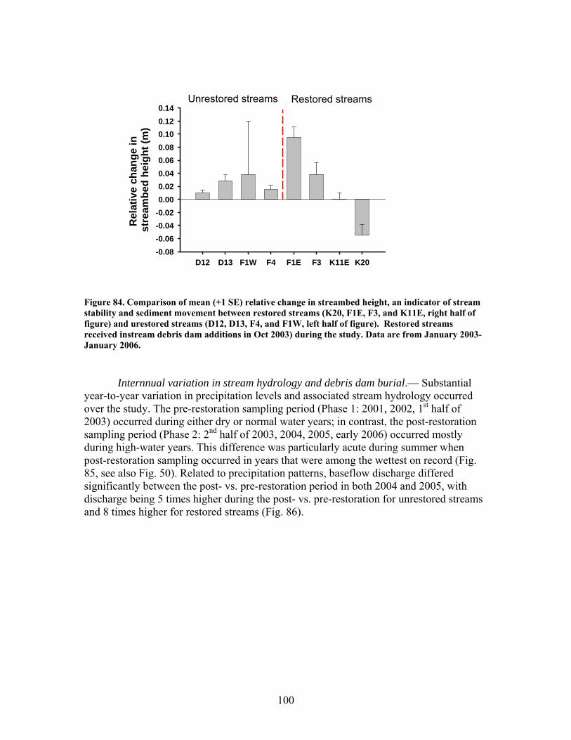
100

D12 D13 F1W F4 F1E F3 K11E K20

Rel

ativ

e ch

ange

in

stre

ambe

d he

ight

(m)

-0.08-0.06-0.04-0.020.000.020.040.060.080.100.120.14

Unrestored streams Restored streams

Figure 84. Comparison of mean (+1 SE) relative change in streambed height, an indicator of stream stability and sediment movement between restored streams (K20, F1E, F3, and K11E, right half of figure) and urestored streams (D12, D13, F4, and F1W, left half of figure). Restored streams received instream debris dam additions in Oct 2003) during the study. Data are from January 2003- January 2006.

Internnual variation in stream hydrology and debris dam burial.— Substantial

year-to-year variation in precipitation levels and associated stream hydrology occurred over the study. The pre-restoration sampling period (Phase 1: 2001, 2002, 1st half of 2003) occurred during either dry or normal water years; in contrast, the post-restoration sampling period (Phase 2: 2nd half of 2003, 2004, 2005, early 2006) occurred mostly during high-water years. This difference was particularly acute during summer when post-restoration sampling occurred in years that were among the wettest on record (Fig. 85, see also Fig. 50). Related to precipitation patterns, baseflow discharge differed significantly between the post- vs. pre-restoration period in both 2004 and 2005, with discharge being 5 times higher during the post- vs. pre-restoration for unrestored streams and 8 times higher for restored streams (Fig. 86).

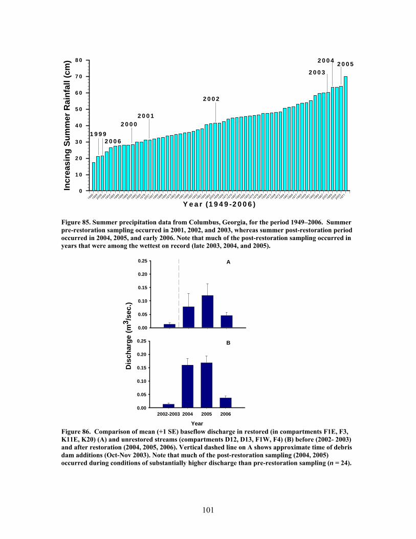
101

Y e a r (1 9 4 9 -2 0 0 6 )1990

19992006

19931954

19851988

19861968

20001982

19951978

20011957

19801998

19841979

19631996

19811960

19971952

19611955

19622002

19581956

19731970

19871983

19501953

19741976

19691959

19751948

19721994

19911966

19771965

19491951

19921964

19672003

19892004

20051971

Incr

easi

ng S

umm

er R

ainf

all (

cm)

0

1 0

2 0

3 0

4 0

5 0

6 0

7 0

8 0

1 9 9 92 0 0 0

2 0 0 1

2 0 0 4

2 0 0 2

2 0 0 32 0 0 5

2 0 0 6

Figure 85. Summer precipitation data from Columbus, Georgia, for the period 1949–2006. Summer pre-restoration sampling occurred in 2001, 2002, and 2003, whereas summer post-restoration period occurred in 2004, 2005, and early 2006. Note that much of the post-restoration sampling occurred in years that were among the wettest on record (late 2003, 2004, and 2005).

Dis

char

ge (m

3 /se

c.)

0.00

0.05

0.10

0.15

0.20

0.25

Year

2002-2003 2004 2005 20060.00

0.05

0.10

0.15

0.20

0.25

A

B

Figure 86. Comparison of mean (+1 SE) baseflow discharge in restored (in compartments F1E, F3, K11E, K20) (A) and unrestored streams (compartments D12, D13, F1W, F4) (B) before (2002- 2003) and after restoration (2004, 2005, 2006). Vertical dashed line on A shows approximate time of debris dam additions (Oct-Nov 2003). Note that much of the post-restoration sampling (2004, 2005) occurred during conditions of substantially higher discharge than pre-restoration sampling (n = 24).

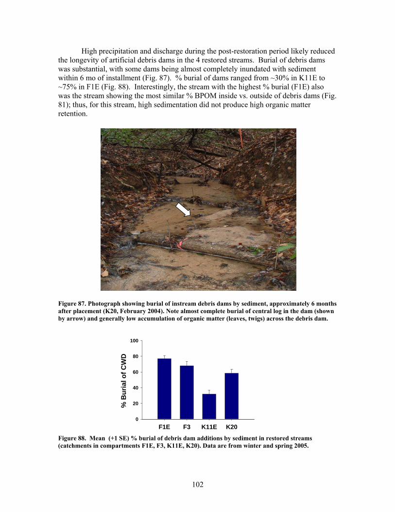
102

High precipitation and discharge during the post-restoration period likely reduced the longevity of artificial debris dams in the 4 restored streams. Burial of debris dams was substantial, with some dams being almost completely inundated with sediment within 6 mo of installment (Fig. 87). % burial of dams ranged from ~30% in K11E to ~75% in F1E (Fig. 88). Interestingly, the stream with the highest % burial (F1E) also was the stream showing the most similar % BPOM inside vs. outside of debris dams (Fig. 81); thus, for this stream, high sedimentation did not produce high organic matter retention.

Figure 87. Photograph showing burial of instream debris dams by sediment, approximately 6 months after placement (K20, February 2004). Note almost complete burial of central log in the dam (shown by arrow) and generally low accumulation of organic matter (leaves, twigs) across the debris dam.

Figure 88. Mean (+1 SE) % burial of debris dam additions by sediment in restored streams (catchments in compartments F1E, F3, K11E, K20). Data are from winter and spring 2005.

F1E F3 K11E K20

% B

uria

l of C

WD

0

20

40

60

80

100

103

Periphyton.—Large increases in several periphyton measures occurred both in unrestored and restored streams in 2004 compared with 2003, and we surmised that high 2004 levels represented, at least in part, a recovery from increased hydrologic disturbance from storms during late 2003. Given these increases across all streams, we assessed periphyton responses to restoration by comparing mean % increases from 2003 to 2004 between restored vs. unrestored streams. Mean % increases in algal biomass (as chlorophyll a concentration) between restored and unrestored streams were significantly higher for restored streams in winter 2004 (p < 0.04) and marginally significant for restored streams in winter 2005 (p < 0.06; Fig. 89A). Differences between restored and unrestored streams were not apparent in spring or summer, although high hydrologic disturbance from elevated stream flows (Fig. 86) and/or high within-treatment variation in chlorophyll a may have reduced detection of restoration effects in these seasons, especially in summer (Fig. 89A). Relative abundance of the disturbance-intolerant diatom Eunotia was a useful indicator of catchment disturbance in the study streams during Phase 1 (Fig. 44). However, % Eunotia did not reveal long-term or ecologically meaningful effects of restorations within the study streams. Differences in % increases in % Eunotia between restored and streams were only significant in winter 2004 (6 months after debris dam additions, p < 0.03; Fig. 89B); thereafter, high within-treatment variation occurred in both restored and unrestored streams. Figure 89. Mean (+1 SE) % increase (from 2003 levels) in season-specific episammic (sand) algal biomass (as log-transformed chlorophyll a concentration, (A) and relative abundance of the diatom Eunotia (B) for restored streams (in compartments F1E, F3, K11E, K20) and unrestored streams (in compartments D12, D13, F1W, F4). Restored streams received instream debris dam additions in Oct-

% In

crea

se in

chl

orop

hyll

a

2

3

4

5

6Restored Unrestored

Winter Spring Autumn Winter2004 2005

A

B

Incr

ease

in %

Eun

otia

0

5

10

15

Restored Unrestored

Winter Spring Summer Winter2004 2005

*

*

104

Nov 2003 and supplemental debris dams (F1E and K20) in Nov 2004. Asterisks indicate significant differences in means between restored and unrestored streams (α= 0.05). Similar to % Eunotia, differences between treatments in % increases of acidobiontic taxa (preferring low streamwater pH), which included Eunotia and other diatom taxa, only were significant in winter 2004 (Fig. 90A). Eunotia is nonmotile, so significantly lower increases in this taxon in restored streams during winter 2004 may have resulted from complementary increases in motile diatom taxa (Fig. 90B), possibly because retention of fine sediments in restored streams favored motile (vs. nonmotile) diatoms. Differences in diatom diversity (as H’) and proportions of epixylic (wood-dwelling) diatom taxa in episammic (sand) samples were not significantly different between restored and unrestored streams in any season (p > 0.05); however, % of diatoms as epixylic (wood-associated) taxa were significantly less variable (as % CV) in restored (vs. unrestored) streams in winter 2004 (Fig. 90C). The latter result suggests that debris dam additions may have increased epixylic diatom abundances, at least shortly after restorations, and thus reduced epixylic diatom heterogeneity in episammic samples.

105

% a

cido

bion

tic ta

xa

-2

0

2

4

6

% m

otile

taxa

-6

-4

-2

0

2

4

6

% w

ood

taxa

CV

-40

-20

0

20

Winter Spring Summer

2004

Figure 90. Mean (+1 SE) % increase (from 2003 levels) in season-specific relative abundance of acidobiontic (low-pH) diatom taxa (A) and motile diatom taxa (B), and % increases in variation (as coefficient of variation, %CV) in epixylic (wood) diatom taxa (C) occurring in episammic (sand) habitats for restored streams (in compartments F1E, F3, K11E, K20) and unrestored streams (in compartments D12, D13, F1W, F4). Restored streams received instream debris dam additions in Oct-Nov 2003 and supplemental debris dams (F1E and K20) in Nov 2004. Differences between restored and unrestored streams only were significant in Winter 2004, 6 months after restorations. Asterisks indicate significant differences in means between restored and unrestored streams.

Restored

Unrestored

B

A

C

*

*

*

106

Similar to patterns observed for % BPOM (Fig. 81), examination of microhabitat-specific differences in chlorophyll a concentration inside vs. outside of debris dams for the 4 restored streams revealed a generally positive effect of restoration on periphyton biomass. Using this approach, chlorophyll a concentration was significantly or marginally significantly higher inside vs. outside the debris dams in 3 of the 4 restored streams (F1E, F3, and K11E, p = 0.003, 0.059, and 0.010, respectively; Fig. 91). Thus, although somewhat variable among streams and for reach-level measures (e.g., Fig. 89A), in-stream debris dam additions appeared to have an overall positive effect on local periphyton accrual in restored streams. However, dam additions had only transitory effects on diatom composition, which likely occurred because of the minimal effects of restorations on streamwater pH, a critical environmental factor for many diatoms. Eunotia and other acidobiontic diatom taxa require low-pH environments (Patrick and Reimer 1966, 1975, Camburn and Charles 2000), conditions that at Ft. Benning appear to occur only in minimally disturbed streams (Fig. 24). Therefore, fundamental changes toward increased dominance by Eunotia and other acidobiontic taxa in restored streams are unlikely to occur unless management practices are sufficient to reduce streamwater pH to levels found in minimally disturbed streams at Ft. Benning.

F3 K20F1E K11E

Chl

orop

hyll

a

0

25

50

150225

Inside Debris DamsOutside Debris Dams

Stream

Figure 91. Mean (+1 SE) benthic chlorophyll a concentration (µg/L) for restored catchments (streams in compartments F1E, F3, K11E, K20) inside vs. outside of debris dams (see text). Restored streams received debris dam additions in Oct-Nov 2003 and supplemental debris dams (F1E and K20) in Nov 2004. Data are from September 2006 (n = 4).

Benthic macroinvertebrates.—Response of benthic macroinvertebrate to debris

dam additions was limited to combinations of particular seasons and metrics. Preliminary analysis of 2004 and 2005 data suggested that winter responses were stronger than summer or spring responses, but final analyses that included 2006 data revealed that effects of debris dam additions occurred in multiple seasons, depending on metric. Density of taxa in aquatic insect orders Ephemeroptera, Plecoptera, and Trichoptera (EPT), a useful indicator of catchment disturbance in Phase 1, showed a significant increase (F = 8.25, p = 0.002) in restored streams in winter compared to no significant

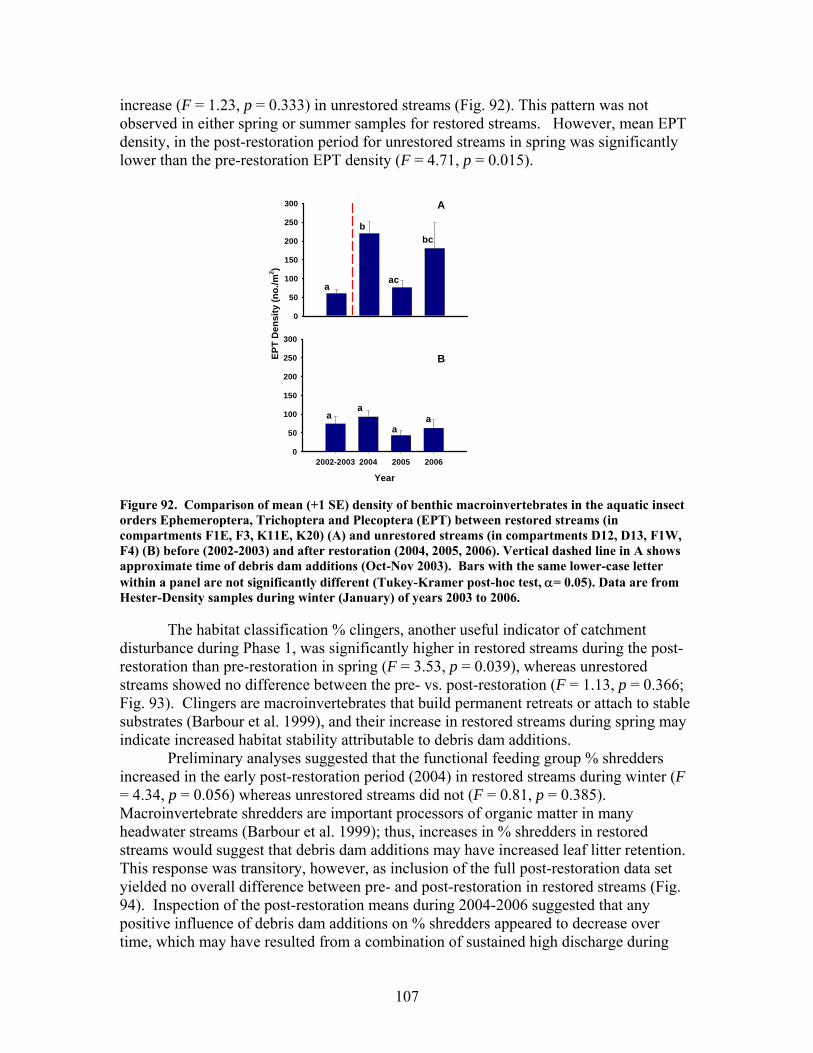
107

increase (F = 1.23, p = 0.333) in unrestored streams (Fig. 92). This pattern was not observed in either spring or summer samples for restored streams. However, mean EPT density, in the post-restoration period for unrestored streams in spring was significantly lower than the pre-restoration EPT density (F = 4.71, p = 0.015).

0

50

100

150

200

250

300

Year

2002-2003 2004 2005 2006

EPT

Den

sity

(no.

/m2 )

0

50

100

150

200

250

300

A

B

a

b

ac

bc

aa

aa

Figure 92. Comparison of mean (+1 SE) density of benthic macroinvertebrates in the aquatic insect orders Ephemeroptera, Trichoptera and Plecoptera (EPT) between restored streams (in compartments F1E, F3, K11E, K20) (A) and unrestored streams (in compartments D12, D13, F1W, F4) (B) before (2002-2003) and after restoration (2004, 2005, 2006). Vertical dashed line in A shows approximate time of debris dam additions (Oct-Nov 2003). Bars with the same lower-case letter within a panel are not significantly different (Tukey-Kramer post-hoc test, α= 0.05). Data are from Hester-Density samples during winter (January) of years 2003 to 2006.

The habitat classification % clingers, another useful indicator of catchment disturbance during Phase 1, was significantly higher in restored streams during the post-restoration than pre-restoration in spring (F = 3.53, p = 0.039), whereas unrestored streams showed no difference between the pre- vs. post-restoration (F = 1.13, p = 0.366; Fig. 93). Clingers are macroinvertebrates that build permanent retreats or attach to stable substrates (Barbour et al. 1999), and their increase in restored streams during spring may indicate increased habitat stability attributable to debris dam additions.

Preliminary analyses suggested that the functional feeding group % shredders increased in the early post-restoration period (2004) in restored streams during winter (F = 4.34, p = 0.056) whereas unrestored streams did not (F = 0.81, p = 0.385). Macroinvertebrate shredders are important processors of organic matter in many headwater streams (Barbour et al. 1999); thus, increases in % shredders in restored streams would suggest that debris dam additions may have increased leaf litter retention. This response was transitory, however, as inclusion of the full post-restoration data set yielded no overall difference between pre- and post-restoration in restored streams (Fig. 94). Inspection of the post-restoration means during 2004-2006 suggested that any positive influence of debris dam additions on % shredders appeared to decrease over time, which may have resulted from a combination of sustained high discharge during

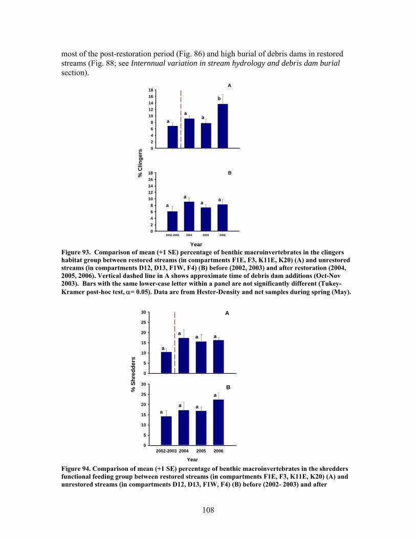
108

most of the post-restoration period (Fig. 86) and high burial of debris dams in restored streams (Fig. 88; see Internnual variation in stream hydrology and debris dam burial section).

2002-2003 2004 2005 2006

% C

linge

rs

02468

1012141618

Year

02468

1012141618

aa

a

b

a

aa a

A

B

Figure 93. Comparison of mean (+1 SE) percentage of benthic macroinvertebrates in the clingers habitat group between restored streams (in compartments F1E, F3, K11E, K20) (A) and unrestored streams (in compartments D12, D13, F1W, F4) (B) before (2002, 2003) and after restoration (2004, 2005, 2006). Vertical dashed line in A shows approximate time of debris dam additions (Oct-Nov 2003). Bars with the same lower-case letter within a panel are not significantly different (Tukey-Kramer post-hoc test, α= 0.05). Data are from Hester-Density and net samples during spring (May).

0

5

10

15

20

25

30

Year

2002-2003 2004 2005 2006

% S

hred

ders

0

5

10

15

20

25

30

A

B

a

aa a

aa a

a

Figure 94. Comparison of mean (+1 SE) percentage of benthic macroinvertebrates in the shredders functional feeding group between restored streams (in compartments F1E, F3, K11E, K20) (A) and unrestored streams (in compartments D12, D13, F1W, F4) (B) before (2002- 2003) and after

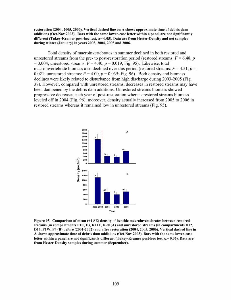
109

restoration (2004, 2005, 2006). Vertical dashed line on A shows approximate time of debris dam additions (Oct-Nov 2003). Bars with the same lower-case letter within a panel are not significantly different (Tukey-Kramer post-hoc test, α= 0.05). Data are from Hester-Density and net samples during winter (January) in years 2003, 2004, 2005 and 2006.

Total density of macroinvertebrates in summer declined in both restored and

unrestored streams from the pre- to post-restoration period (restored streams: F = 6.48, p = 0.004; unrestored streams: F = 4.40, p = 0.019; Fig. 95). Likewise, total macroinvertebrate biomass also declined over this period (restored streams: F = 4.51, p = 0.021; unrestored streams: F = 4.00, p = 0.035; Fig. 96). Both density and biomass declines were likely related to disturbance from high discharge during 2003-2005 (Fig. 38). However, compared with unrestored streams, decreases in restored streams may have been dampened by the debris dam additions. Unrestored streams biomass showed progressive decreases each year of post-restoration whereas restored streams biomass leveled off in 2004 (Fig. 96); moreover, density actually increased from 2005 to 2006 in restored streams whereas it remained low in unrestored streams (Fig. 95).

A

B

Den

sity

(no.

/m2 )

0200400600800

100012001400160018002000

a

b b

ab

Year2001-2002 2004 2005 2006

0

200

400

600

800

1000

1200

1400

a

abb

ab

Figure 95. Comparison of mean (+1 SE) density of benthic macroinvertebrates between restored streams (in compartments F1E, F3, K11E, K20 (A) and unrestored streams (in compartments D12, D13, F1W, F4 (B) before (2001-2002) and after restoration (2004, 2005, 2006). Vertical dashed line in A shows approximate time of debris dam additions (Oct-Nov 2003). Bars with the same lower-case letter within a panel are not significantly different (Tukey-Kramer post-hoc test, α= 0.05). Data are from Hester-Density samples during summer (September).

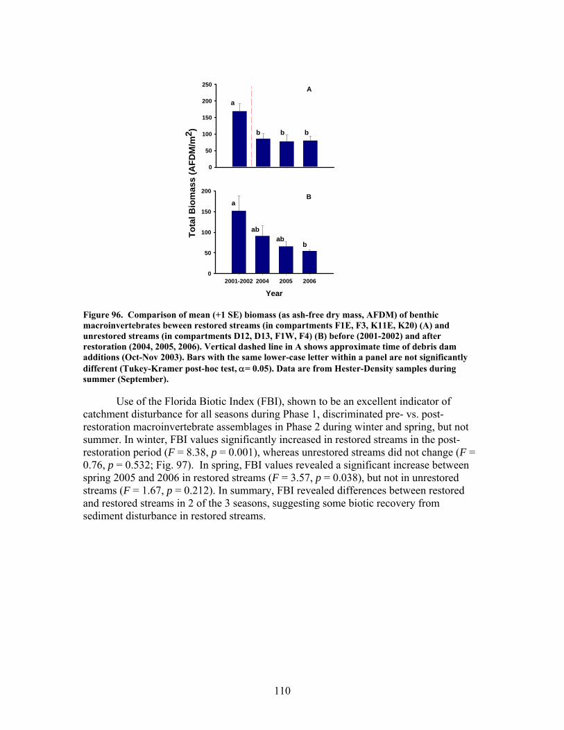
110

Tota

l Bio

mas

s (A

FDM

/m2 )

0

50

100

150

200

250

Year2001-2002 2004 2005 2006

0

50

100

150

200

a

b b b

a

abab

b

A

B

Figure 96. Comparison of mean (+1 SE) biomass (as ash-free dry mass, AFDM) of benthic macroinvertebrates beween restored streams (in compartments F1E, F3, K11E, K20) (A) and unrestored streams (in compartments D12, D13, F1W, F4) (B) before (2001-2002) and after restoration (2004, 2005, 2006). Vertical dashed line in A shows approximate time of debris dam additions (Oct-Nov 2003). Bars with the same lower-case letter within a panel are not significantly different (Tukey-Kramer post-hoc test, α= 0.05). Data are from Hester-Density samples during summer (September).

Use of the Florida Biotic Index (FBI), shown to be an excellent indicator of catchment disturbance for all seasons during Phase 1, discriminated pre- vs. post-restoration macroinvertebrate assemblages in Phase 2 during winter and spring, but not summer. In winter, FBI values significantly increased in restored streams in the post-restoration period (F = 8.38, p = 0.001), whereas unrestored streams did not change (F = 0.76, p = 0.532; Fig. 97). In spring, FBI values revealed a significant increase between spring 2005 and 2006 in restored streams (F = 3.57, p = 0.038), but not in unrestored streams (F = 1.67, p = 0.212). In summary, FBI revealed differences between restored and restored streams in 2 of the 3 seasons, suggesting some biotic recovery from sediment disturbance in restored streams.

111

2002-2003 2004 2005 2006Fl

orid

a B

iotic

Inde

x0

5

10

15

20

25

Year

2002-2003 2004 2005 20060

5

10

15

20

25

A

B

a aab

b

aa

a a

Figure 97. Comparison of mean (+1 SE) values of the Florida Biotic Index between restored streams (in compartments F1E, F3, K11E, K20) (A) and unrestored streams (in compartments D12, D13, F1W, F4) (B) before (2002, 2003) and after restoration (2004, 2005, 2006). Vertical dashed line on A shows approximate time of debris dam additions (Oct-Nov 2003). Bars with the same lower-case letter within a panel are not significantly different (Tukey-Kramer post-hoc test, α= 0.05). Data are from Hester-Density and net samples during winter (January).

In addition to comparing macroinvertebrate assemblages between restored and

unrestored stream reaches, we conducted supplemental benthic sampling near debris dams in the 4 restored streams to examine fine-scale (microhabitat) influences of debris dam additions on benthic assemblages. We used a modified T-sampler (PVC, 10.8 cm diameter, area = 91.6 cm2) inside (Fig. 80A) and outside (as controls; Fig. 80B) of debris dams, pooling 3 T-samples per site (total sampled area = 274.8 cm2 per location), with 4 sites per stream. Sampling was done in May 2004 and September 2006 (6 and 35 months after restorations, respectively).

Results from 2004 samples (6 months after debris dam additions) indicated that macroinvertebrate clinger richness (number of macroinvertebrate species that cling to hard substrates, Barbour et al. 1999), Diptera richness (number of taxa in the order Diptera), and total richness (number of total macroinvertebrate taxa) did not significantly differ inside vs. outside debris dams (Fig. 98). In contrast, macroinvertebrate H’, total density, and/or total biomass were higher inside than outside debris dams in 3 of the 4 restored streams (K20, F3, and F1E). However, the restored stream with the highest amount of pre-addition CWD (K11E; Fig. 76) and bed stability (Fig. 83) showed the opposite pattern, with significantly higher density and H’ outside (vs. inside) debris dams (Fig. 98). Restored streams in more disturbed catchments with less stable beds (K20, F3, and F1E) increased microhabitat stability associated with debris dams favoring colonization of invertebrates in close proximity to wood. One explanation for this

112

counterintuitive result is that K11E was the least-disturbed restored stream and had sufficient natural wood habitat outside of the artificial debris dams afforded by the stable beds. Moreover, addition of debris dams in K11E formed deep pools (personal observations), which may have actually decreased microhabitat quality for macroinvertebrates in close proximity to debris dams and, thus, increased relative quality of benthic habitats outside of debris dams.

In contrast, results from 2006 samples (35 months after debris dam additions) showed virtually no difference in the above metrics inside versus outside of debris dams for the 4 restored streams. Only taxa richness differed significantly between microhabitats, and for only 1 stream (K20, Fig. 99). Comparisons of values of individual metrics between years are tenuous because samples were taken in different seasons (2004 spring, 2006 summer). Nevertheless, these results suggest that any increase in habitat heterogeneity that was provided by the restoration shortly after debris dams were added in 2003 and, thus, any enhancement of microhabitat diversity and associated biotic integrity in 2004, appeared to have attenuated by the end of the study (2006).

Biomass

Stream

K20 F1E F3 K11E

Bio

mas

s (m

g m

-2)

0

1000

2000

3000

4000Density

Stream

K20 F1E F3 K11E

Den

sity

(# m

-2)

0

1e+4

2e+4

3e+4

4e+4

5e+4Diversity

Stream

K20 F1E F3 K11E

H'

0.0

0.2

0.4

0.6

0.8

1.0

1.2

Clinger richness

Num

ber c

linge

rs

0

1

2

3

4

5

Inside debris damOutside debris dam

Diptera richness

Num

ber D

ipte

ra

0

5

10

15

20

25Taxa richness

Num

ber t

axa

05

101520253035

**

** *

*

Figure 98. Mean (+1 SD) benthic macroinvertebrate measures (number of species of invertebrates that cling to hard substrates [Clinger richness], number of taxa in the order Diptera [Diptera richness], number of total taxa [Taxa richness], Shannon diversity [Diversity], total number of invertebrates [Density], and total invertebrate biomass [Biomass] inside vs. outside of artificial debris dam additions. Restored streams received instream debris dam additions in Oct-Nov 2003 and supplemental debris dams (F1E and K20) in Nov 2004. Streams arranged on x-axis in order of increasing amounts of natural (pre-addition) CWD. Asterisks indicate significant differences between inside and outside measures. Data are from T-samples during spring (May) 2004.

113

Figure 99. Mean (+1 SD) benthic macroinvertebrate measures (number of species of invertebrates that cling to hard substrates [Clinger richness], number of taxa in the order Diptera [Diptera richness], number of total taxa [Taxa richness], Shannon diversity [Diversity], total number of invertebrates [Density], and total invertebrate biomass [Biomass] inside vs. outside of artificial debris dam additions. Restored streams received instream debris dam additions in Oct-Nov 2003 and supplemental debris dams (F1E and K20) in Nov 2004. Streams arranged on x-axis in order of increasing amounts of natural (pre-addition) CWD. Asterisks indicate significant differences between inside and outside measures. Data are from T-samples during summer (September) 2006.

Clinger richness

K20 F1E F3 K11E

Num

ber c

linge

rs

0

1

2

3

4

5

Inside debris damOutside debris dam

Diptera richness

K20 F1E F3 K11E

Num

ber D

ipte

ra

02468

101214

Taxa richness

K20 F1E F3 K11E

Num

ber t

axa

02468

1012141618

Diversity

Stream

K20 F1E F3 K11E

H'

0.0

0.2

0.4

0.6

0.8Density

Stream

K20 F1E F3 K11E

Den

sity

(no.

/m2 )

0500

100015002000250030003500

Biomass

Stream

K20 F1E F3 K11EB

iom

ass

(mg/

m2 )

0

500

1000

1500

2000

*

114

Concluding summary: Riparian restorations.—Although restoration efforts did result in decreased sedimentation rates, there were no clear indications of recovery responses in productivity, nutrient cycling, or community composition at this point. Fine root standing crop biomass and fine root nutrients may be more sensitive to changes in sedimentation, as there were indications of improved growth and nutrient levels. Understory vegetation may also serve as an early indicator of community recovery in areas where it is a significant component of the plant community. There is a tendency for treatment sites F3 and D12 to respond differently than K11 as evidenced by ANPP, belowground production, standing crops of live & dead roots, and understory species composition results. Data from Site F3 suggested that a shift in resource allocation from above- to belowground may have occurred in terms of production and the standing crop of live roots. Similarly, D12 also exhibited greater live root biomass following restoration.

It is possible that variation in precipitation among years is driving vegetation and biogeochemical responses on the treatment plots to a greater extent than the restoration treatments. In addition, it is likely that some vegetation and biogeochemical responses to restoration may require a longer time frame to become manifested (measurably) than has transpired.

In-stream restorations.—The in-stream restorations have resulted in changes in hydrodynamic conditions (increase in water residence times), increase in nutrient uptake rates, increase in gross primary production (spring only) and ecosystem respiration rates (all seasons), and increase in retention of benthic organic matter. Positive responses of stream biota and habitat variables to debris dam additions also were observed in restored streams during the study, including increased relative abundance of BPOM, increased algal biomass, and enhancements in several benthic macroinvertebrate measures (EPT density, % clingers, FBI score) in at least some of the restored streams. Contrary to expectation, restorations produced no similar positive effects on CWD accumulation, increased streambed stability, increased % Eunotia diatoms, and several macroinvertebrate richness measures (no. of EPT taxa, no. of Chironomidae taxa, no. of Tanytarsini taxa, no. of clinger taxa) shown to be useful indicators of catchment disturbance from land use in Phase 1.

At least some of these disparate findings appeared to result from in-stream restorations being compromised by high precipitation and stream discharge, and associated debris dam burial by sediment during much of the post-restoration period. Significant declines in benthic macroinvertebrate density and biomass from pre- to post-restoration periods in both restored and unrestored streams strongly suggest that hydrologic disturbance may have negatively influenced stream habitat and biotic conditions and, thus, muted the overall impact of restorations on stream biotic integrity. If true, then the efficacy of restorations using in-stream debris dams to enhance biotic recovery in disturbed streams at Ft. Benning may depend on antecedent and current hydrologic regimes and their influence on stream communities.

115

TRANSITION: DISTURBANCE INDICATORS AND RESTORATION PROTOCOLS Disturbance assessment indicators and measurements Based on our study findings, below we summarize what we believe to be the most useful disturbance assessment measurements (indicators) for riparian and stream ecosystems (Table 10). Table 10. Summary of most useful disturbance indicators/measurements. Indicator/measurement Rationale Method (references) Riparian vegetation: Leaf area index Higher levels of sedimentation

often cause crown dieback and loss of foliar biomass. Consequently, the foliar surface area declines resulting in lower production of photosynthate.

Area to weight ratios are estimated by determining surface areas on subsamples of litterfall and then expanding those estimates to an area basis using total, annual litterfall dry weights per hectare (Pearcy et al. 1989).

Riparian soils: Current sedimentation rates

Current sedimentation rates of approximately 1.0 cm/yr have been linked to LAI declines and increases in overstory mortality. It is suggested that current rates reflect a preferable method compared to historic rates during periods with average and higher precipitation levels.

Erosion pin method – Steel welding rods (marked with notches or metal washers) are inserted into soil until the notch or washer is at groundline. Soil export or accumulation is measured in reference to changes in the soil surface relative to the marker.

Historic sedimentation rates

Historic sedimentation rates of 0.3 cm/yr over the past 25 years have been associated with declines in riparian forest NPP and rates of biogeochemical cycles. Historic sedimentation rates are likely to be stronger indicators of decline in years with less than average precipitation.

Dendrogeomorphic approach – Buried bases of live, standing trees are excavated to the root collar and ages determined at root collar and soil surface. Measurement of the depth of burial and difference in ages at the two positions provides an estimate of the rate of sediment accumulation over the time period (Hupp and Morris 1990).

Stream water quality indicators:

Suspended sediment concentration

Disturbances often result in large increases in suspended sediment concentrations (particularly during storms) due to increased erosion from uplands or reduced stream bank

Filter 0.1 to 0.5 L of water through pre-combusted and tared glass fiber filters (Whatman GFF), dry (80ºC for 2 d), weigh, combust (500ºC for 12 h), rewet material on filters and dry, and

116

stability. reweigh (APHA 1992). Nutrient concentration Disturbances can result in

increases in ammonium, nitrate, or phosphate concentrations due to losses from terrestrial ecosystems or reduced uptake in streams. Increases in input of clay-rich sediments to streams can also reduce phosphate concentrations due to increased sorption to sediments.

Analysis performed on filtered water (Whatman GFF filters). Ammonium by standard phenate colorimetry, nitrate by Cd-Cu reduction and azo dye colorimetry or by ion chromatography, phosphate by ascorbic acid-molybdenum blue colorimetry (APHA 1992).

Stream metabolism indicators:

Diurnal dissolved oxygen concentration profiles

Disturbances involving increased sediment input and deposition in streams can result in reduced rates of metabolism (gross primary productivity, respiration) which can be identified by changes in the diurnal amplitude and saturation level of dissolved oxygen

Measurement of water temperature and dissolved oxygen concentration at ≤ 15-minute intervals using YSI sondes equipped with optical dissolved oxygen sensors (Mulholland et al. 2005)

Stream habitat indicators:

Streambed instability Sediment inputs from upland sources and in-stream sediment movement from historical disturbance can cause stream bed instability which can be observed by changes in stream bed height.

Measurement of streambed height through the use of multiple, fixed-point transects each perpendicular to the stream flow, with points measured every 10-20cm six times a year (Maloney et al. 2005).

Stream flashiness Disturbance in uplands in the form of bare ground as well as reduced rainfall infiltration into the ground due to soil compaction by heavy equipment increases overland flow subsequently increases stream flashiness

Stream flashiness estimated from recession coefficients of several storm hydrographs, measured by an ISCO ultrasonic flow module (Model 750) and series portable sample (Model 6700); depth and velocity taken ever 30 min to 1 h over a 4-h period (Maloney et al. 2005).

Coarse wood debris (CWD) relative abundance

Disturbance from increase flashiness and stream bed sediment movement can result in the decrease CWD abundance, either by burial or displacement downstream, which in turn may decrease in-stream habitat availability for biota and retention of benthic

Quantification of the relative abundance of CWD is accomplished by measuring all wood, >2.5 cm in diameter, from the upper 10 cm of the substrate to the bankfull height of the stream channel across 15 cross-stream transects space longitudinally 5 m apart

117

particulate organic matter (BPOM).

(Maloney et al. 2005).

Benthic particulate organic matter (BPOM) relative abundance

Disturbance from increased stream flashiness and low CWD can result in the decrease in retention of BPOM which can be identified by a decrease in the % BPOM of the stream bottom.

Measured using sediment cores (PVC pipe, area = 2.01 cm2, 10-cm depth) to quantify proportion of BPOM, three samples per stream every 2-4 months. Samples dried, weighed, ashed (at 550 C), and then desiccated and reweighed to determine % BPOM as ash-free dry mass (AFDM, Maloney et al. 2005).

Stream biotic indicators:

Chironomidae richness Disturbance has been shown to substantially decrease taxa richness of benthic macroinvertebrates by direct mortality or indirectly through habitat loss. In sandy streams, chironomid midges are usually most diverse aquatic insect group, thus their richness is most likely to show impacts from catchment disturbance.

Measurement of Chironomidae richness done by taking seasonal samples from multiple sites within a stream, through use of artificial substrate samplers (e.g., Hester-Dendy multiplates) or kick nets (Maloney and Feminella 2006), or quadrat samplers (e.g., Surber or Hess samplers).

Compositional group measures (% clingers)

Disturbance can decrease benthic macroinvertebrate assemblage measures by decreasing habitat availability for any given group. % clingers is a good measure of sediment disturbance because the primary habitat for this group is hard stable surfaces. As sediment disturbance increase stable habitat decreases, thus decreasing % clingers within the benthic macroinvertebrate assemblage.

Measurement of % clingers done by taking seasonal samples from multiple sites within a stream, through use of artificial substrate samplers (e.g., Hester-Dendy multiplates) or kick nets (Maloney and Feminella 2006), or quadrat samplers (e.g., Surber or Hess samplers).

Density of EPT taxa

Disturbance can substantially decrease density of benthic macroinvertebrates by direct mortality or indirect habitat loss. Density of EPT (Ephemeroptera, Plecoptera, Trichoptera) are usually the most sensitive aquatic insect orders, thus density of EPT taxa is likely to show impacts from catchment disturbance.

Measurement of EPT density done by taking seasonal samples from multiple sites within a stream, through use of fixed-area artificial substrate samplers (e.g., Hester-Dendy multiplates) (Maloney and Feminella 2006) or quadrat samplers (e.g., Surber or Hess samplers).

118

Florida Biotic Index (FBI)

Disturbance from increased sediment inputs can reduce or eliminate sediment-intolerant benthic macroinvertebrate taxa. As disturbance increase the FBI decreases because of loss of intolerant taxa.

Measurement of FBI done by taking seasonal samples from multiple sites within a stream, through use of either artificial substrate samplers (e.g., Hester-Dendy multiplates), kick nets, or or quadrat samplers (e.g., Surber or Hess samplers). Taxa are ranked based on their tolerance category, with 2 being the most sensitive and 0 being the most tolerant (Maloney and Feminella 2006).

Georgia stream condition index (GASCI)

As disturbance from increased sediment inputs reduces habitat quality values of individual benthic macroinvertebrate metrics values also are reduced. With increasing disturbance GASCI takes into account both reductions in biotic parameters and changes in several habitat measures. The greater the reduction in GASCI value the greater the impairment.

Measurement of GASCI done by taking seasonal samples from multiple sites within a stream, through use of either artificial substrate samplers (e.g., Hester-Dendy multiplates) or kick nets. GASCI incorporates multiple metrics such as Chironomidae richness and the FBI, plus habitat measures including channel sinuosity and bank stability (Maloney and Feminella 2006).

Algal biomass (as chlorophyll a concentration)

As catchment disturbance increases benthic algal biomass decreases from scour or burial by sediment. High algal biomass suggests high streambed stability.

Algal biomass sampling by inserting an inverted Petri dish (44 cm3) into sand substrates randomly in 3 run habitats per stream and removing samples with a spatula (Miller 2006). Algal photosynthetic pigments (chlorophyll a) extracted using 90% acetone, determined fluorometrically (Arar and Collins 1992).

Diatom composition (as % Eunotia)

As catchment disturbance increases the average body size of fish decreases.

Diatoms sampled by inserting an inverted a small Petri dish (7 cm3) into sand substrates randomly in 3 run habitats per stream and removing samples with a spatula (Miller 2006). Composition quantified by preserving samples in 2% glutaraldehyde, cleaning diatoms with hydrogen peroxide and nitric acid, slide-mounting them with NaphraxTM, and then identifying/counting 400–500 valves/stream/season (1000×), mainly using keys in Camburn and Charles (2000) and Patrick

119

and Reimer (1966, 1975).

Stream fish body size

As catchment disturbance increases the average body size of fish decreases. The 2 numerically dominant fish species in Fort Benning streams (Pteronotropis euryzonus and Semotilus thoreauianus) show smaller body sizes as catchment disturbance increases.

Mean body size measured as standard length (SL) of stream fishes collected seasonally taken from pool and run microhabitat using a Smith-Root LR-24 fish electroshocker (Maloney et al. 2006), and

Proportion of the fish assemblage as the broadstripe shiner (Pteronotropis euryzonus

As sediment disturbance increases within a watershed the proportion the fish assemblage as Pterontropis euryzonus decreases.

Measurement of proportion of the fish assemblage as Pteronotropis euryzonus calculated from seasonal samples taken from both pool and run microhabitat using a Smith-Root LR-24 fish electroshocker (Maloney et al. 2006).

Proportion of the fish assemblage as the Dixie chub (Semotilus thoreauianus)

As sediment disturbance increases within a watershed the proportion the fish assemblage as Semotilus thoreauianus increases.

Measurement of proportion of the fish assemblage as Semotilus thoreauianus calculated from seasonal samples taken from both pool and run microhabitat using a Smith-Root LR-24 fish electroshocker (Maloney et al. 2006).

Ecosystem Restoration Protocols and Costs Restoration protocols and costs are summarized in Table 11 below. It should be noted, however, that the costs presented have a high degree of uncertainty, depending on the degree of disturbance and the local cost of labor since these restoration approaches are labor-intensive.

Restoration of ephemeral stream channels below intersections with dirt roads on side slopes and ridge lines is more important than any other factor associated with sustaining riparian and aquatic systems at Ft. Benning. Non-degraded, vegetated ephemeral channels serve as filters for sediment that otherwise would move downslope and accumulate in riparian areas and in streams. Our research has shown that accumulation is directly responsible for vegetation decline and mortality in downslope topographic positions. In addition, degraded ephemeral channels represent a primary conduit for movement of sediment into stream channels.

Restoration of perennial stream channels using in-stream artificial debris dams to enhance stream habitat and biota may require 1) regular (e.g., annual) supplementation of debris dams in manipulated reaches to augment loss of debris dams from downstream displacement and/or burial by sediment, 2) a larger manipulated reach than was used in our study (i.e., >>150-m of restored reach for a 1st–2nd-order stream) to help stabilize upstream sediment sources, or 3) a combination of the previous 2 approaches. Regular

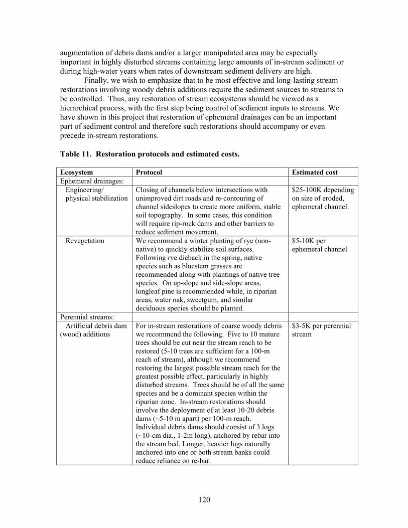
120

augmentation of debris dams and/or a larger manipulated area may be especially important in highly disturbed streams containing large amounts of in-stream sediment or during high-water years when rates of downstream sediment delivery are high.

Finally, we wish to emphasize that to be most effective and long-lasting stream restorations involving woody debris additions require the sediment sources to streams to be controlled. Thus, any restoration of stream ecosystems should be viewed as a hierarchical process, with the first step being control of sediment inputs to streams. We have shown in this project that restoration of ephemeral drainages can be an important part of sediment control and therefore such restorations should accompany or even precede in-stream restorations. Table 11. Restoration protocols and estimated costs. Ecosystem Protocol Estimated cost Ephemeral drainages: Engineering/ physical stabilization

Closing of channels below intersections with unimproved dirt roads and re-contouring of channel sideslopes to create more uniform, stable soil topography. In some cases, this condition will require rip-rock dams and other barriers to reduce sediment movement.

$25-100K depending on size of eroded, ephemeral channel.

Revegetation We recommend a winter planting of rye (non-native) to quickly stabilize soil surfaces. Following rye dieback in the spring, native species such as bluestem grasses are recommended along with plantings of native tree species. On up-slope and side-slope areas, longleaf pine is recommended while, in riparian areas, water oak, sweetgum, and similar deciduous species should be planted.

$5-10K per ephemeral channel

Perennial streams: Artificial debris dam (wood) additions

For in-stream restorations of coarse woody debris we recommend the following. Five to 10 mature trees should be cut near the stream reach to be restored (5-10 trees are sufficient for a 100-m reach of stream), although we recommend restoring the largest possible stream reach for the greatest possible effect, particularly in highly disturbed streams. Trees should be of all the same species and be a dominant species within the riparian zone. In-stream restorations should involve the deployment of at least 10-20 debris dams (~5-10 m apart) per 100-m reach. Individual debris dams should consist of 3 logs (~10-cm dia., 1-2m long), anchored by rebar into the stream bed. Longer, heavier logs naturally anchored into one or both stream banks could reduce reliance on re-bar.

$3-5K per perennial stream

121

122

LITERATURE CITED Arar, E.J., and G.B. Collins. 1992. In vitro determination of chlorophyll-a and pheophytin-a in marine and freshwater phytoplankton by fluorescence. Environmental Monitoring and Support Laboratory. U.S. Environmental

Protection Agency. American Public Health Association (APHA), 1992. Standard methods for the

examination of water and waste water, 18th edition. American Public Health Association, Washington, DC.

Barbour, M. T., J. Gerritsen, B. D. Snyder, and J. B. Stribling. 1999. Rapid bioassessment

protocols for use in streams and wadeable rivers: periphyton, benthic macroinvertebrates, and fish 2nd edition. U.S.EPA Office of Water Regulation and Standards, Washington DC. EPA 841-B-99-002.

Bencala, K. E., and R. A. Walters. 1983. Simulation of solute transport in a mountain

pool-and-riffle stream: a transient storage model. Water Resour. Res. 19:718-724.

Bott, T. L., 1996. Primary productivity and community respiration, pp. 533-556. In: F.

R. Hauer and G. A. Lamberti, Methods in Stream Ecology. Academic Press, San Diego.

Camburn, K. E. and D. F. Charles. 2000. Diatoms of Low-Alkalinity Lakes in the Northeastern United States. Special Publication 18. The Academy of Natural Sciences of Philadelphia, Philadephia, Pennsylvania. Carpenter, S. R., T. M. Frost, D. Heisey, and T. K. Kratz. 1989. Randomized

intervention analysis and the interpretation of whole-ecosystem experiments. Ecology 70:1142-1152.

Correll, D. L., R. E. Jordan, and D. E. Weller. 1999a. Precipitation effects on sediment

and associated nutrient discharges from Rhode River watersheds. Journal of Environmental Quality 28:1897-1907.

Correll, D. L., R. E. Jordan, and D. E. Weller. 1999b. Transport of nitrogen and

phosphorus from Rhode River watersheds during storm events. Water Resources Research 35:2513-2521.

Evans, C. and T. D. Davies. 1998. Causes of concentration/discharge hysteresis and its

potential as a tool for analysis of episode hydrochemistry. Water Resources Research 34:129-137.

Florida Department of Natural Resources. 1996. Standard operating procedures for

biological assessment. (available from FL Department of Environmental Protection, Tallahassee, Florida).

123

Georgia Department of Natural Resources. 2002. Standard operating procedures (SOP),

freshwater macroinvertebrate biological assessment. (available from GA Department of Natural Resources, Water Protection Branch, Watershed Planning and Monitoring Program, Ambient Monitoring Unit, 4220 International Parkway, Suite 101, Atlanta, Georgia).

Gordon, N. D., T. A. McMahon, and B. L.Finlayson. 1992. Stream hydrology, an introduction for ecologists. John Wiley and Sons, NY.

Gregory S. V., F. J. Swanson, W. A. McKee, and K. W. Cummins. 1991. An ecosystem

perspective of riparian zones. BioScience 41:540-551. Hardison, B. S. and J. B. Layzer. 2001. Relations between complex hydraulics and the

localized distribution of mussels in three regulated rivers. Regulated Rivers: Research and Management 17:77-84.

Hart, D. R. 1995. Parameter estimation and stochastic interpretation of the transient

storage model for solute transport in streams. Water Resour. Res. 29: 89-98. Hart, S. C., J. M. Stark, E. A. Davidson, and M. K. Firestone. 1994. Nitrogen

mineralization, immobilization, and nitrification. Pages 985-1018 in R. W. Weaver, J. S. Angle, and P. S. Bottomley, editors. Methods of Soil Analysis. SSSA, Madison, WI.

Hill A. R. 1996. Nitrate removal in stream riparian zones. Journal of Environmental

Quality 25:743-755. Houser, J. N, P. J. Mulholland, and K. O. Maloney. 2005. Catchment disturbance and

stream metabolism: patterns in ecosystem respiration and gross primary production along a gradient of upland soil and vegetation disturbance. J. N. Am. Benthol. Soc. 24: 538-552.

Houser, J. N., P. J. Mulholland, and K. O. Maloney. 2006. Upland disturbance affects

headwater stream nutrients and suspended sediments during baseflow and stormflow. Journal of Environmental Quality 35: 352-365.

Hupp, C. R., and E. E. Morris. 1990. A dendrogeomorphic approach to measurement of

sedimentation in a forested wetland, Black Swamp, Arkansas. Wetlands 10:107-124.

Hurlbert, S. H. 1984. Pseudoreplication and the design of ecological field experiments.

Ecological Monographs 54:187-211. Jordan, T. E., D. L. Correll, and D. E. Weller. 1997a. Effects of agriculture on

discharges of nutrients from Coastal Plain watersheds of Chesapeake Bay. Journal of Environmental Quality 26:836-848.

124

Jordan, T. E., D. L. Correll, and D. E. Weller. 1997b. Relating nutrient discharges from

watersheds to land use and streamflow variability. Water Resources Research 33:2579-2590.

Kleiss, B. A. 1993. Method for measuring sedimentation rates in bottomland hardwood

(BLH) wetlands. Wetlands Research Program Technical Note SD-CP-4.1, U.S. Army Engineer Waterways Experiment Station, Vicksburg, MS, USA.

Klemm, D.J., P.A. Lewis, F. Fulk, and J.M. Lazorchak. 1990. Macroinvertebrate field

and laboratory methods for evaluating the biological integrity of surface waters. U.S. Environmental Protection Agency, Office of Modeling, Monitoring Systems, and Quality Assurance. Washington D. C. EPA/600/4-90/030.

Kutka F. J. and C. Richards. 1997. Relating diatom assemblage structure to stream habitat

quality. Journal of the North American Benthological Society 15:469-480. Lenat D. R. 1993. A biotic index for the southeastern United States: derivation and list of

tolerance values, with criteria for assigning water-quality ratings. Journal of the North American Benthological Society 12:279-290.

Liu, Z-J., D. E. Weller, D. L. Correll, and T. E. Jordan. 2000. Effects of land cover and

geology on stream chemistry in watersheds of the Chesapeake Bay. Journal of the American Water Resources Association 36:1349-1365.

Maloney, K. O, P.J. Mulholland, and J.W. Feminella. 2005. The effects of catchment-

scale military land use on stream physical and organic matter variables in small Southeastern Plains catchments (USA). Environmental Management 35:677-691.

Maloney, K. O. and J. W. Feminella. 2006. Evaluation of single- and multi-metric

benthic macroinvertebrate indicators of catchment disturbance over time at the Fort Benning Military Installation, Georgia, USA. Ecological Indicators 6:469-484.

Maloney, K. O., R. M. Mitchell, and J. W. Feminella. 2006. Influence of catchment

disturbance from military training on fish assemblages in small southeastern headwater streams. Southeastern Naturalist 5:393-412.

Miller, S.A. 2006. Relationships between wood and benthic algae: influence of

landscape disturbance and decomposer competition. MSc Thesis, Auburn University.

Morgan, M. D., and R. E. Good. 1988. Stream chemistry in the New Jersey Pinelands:

the influence of precipitation and watershed disturbance. Water Resources Research 24:1091-1100.

125

Morrice, J. A., H. M. Valett, C. N. Dahm, and N. E. Campana. 1997. Alluvial characteristics, groundwater-surface water exchange, and hydrologic retention in headwater streams. Hydrol. Proc. 11: 253-267.

Mozaffari, M., and J. T. Sims. 1994. Phosphorus availability and sorption in an Atlantic

Coastal Plain watershed dominated by animal-based agriculture. Soil Science 157:97-107.

Mulholland, P. J., L. A Yarbro, R. P. Sniffen, and E. J. Kuenzler. 1981. Effects of floods

on nutrient and metal concentrations in a Coastal Plain stream. Water Resources Research 17:758-764.

Mulholland, P. J., J. N. Houser, and K. O. Maloney. 2005. Stream diurnal dissolved

oxygen profiles as indicators of in-stream metabolism and disturbance effects: Fort Benning as a case study. Ecological Indicators 5: 243-252.

Nadelhoffer, K. J., J. D. Aber, and J. M. Melillo. 1985. Fine roots, net primary

productivity, and soil nitrogen availability: A new hypothesis. Ecology 66:1377-1390.

Naiman, R.J., H. Decamps, and M. Pollack. 1993. The role of riparian corridors in

maintaining regional diversity. Ecol. Applications 3:209-212. NCDENR (North Carolina Department of Environmental and Natural Resources), 2003.

Standard operating procedures for benthic macroinvertebrates, http://www.esb.enr.state.nc.us/BAU.html, 44 pp.

O’Brien, A. K., K. C. Rice, M. M. Kennedy, and O. P. Bricker. 1993. Comparison of

episodic acidification of Mid-Atlantic upland and Coastal Plain streams. Water Resources Research 29:3029-3039.

Osborne L. L. and D. A. Kovacic. 1993. Riparian vegetated buffer strips in water-quality

restoration and stream management. Freshwater Biology 29:243-258.

Patrick,R. and C.W. Reimer. 1966. The diatoms of the United States I. Monographs of the Academy of Natural Sciences of Philadelphia, 13. Patrick, R. and C. W. Reimer. 1975. The diatoms of the United States, Vol. 2. Part 1.

Monograph No. 13. Academy of Natural Sciences of Philadelphia, Philadephia, Pennsylvania.

Pearcy, R.W., J.R. Ehleringer, H.A. Mooney, and P.W. Rundel. 1990. Plant Physiological

Ecology: Field Methods and Instrumentation. Chapman and Hall. New York. 457 p.

126

Rabeni C. F. and M. A. Smale. 1995. Effects of siltation on stream fishes and the potential mitigating role of the buffering riparian zone. Hydrobiologia 303:211-219.

Ray, G. A., and W. F. Megahan. 1979. Measuring cross sections using a sag tape: a

generalized procedure. General Technical Report INT-47. Intermountain forest and range experiment station, Forest Service, U. S. Department of Agriculture, Ogden, Utah.

Rose, S., and N. E. Peters. 2001. Effects of urbanization on streamflow in the Atlanta

area (Georgia, USA): a comparative hydrological approach. Hydrological Processes 15:1441-1457.

Rosenberg, D.M. and V.H. Resh, editors. 1993. Freshwater biomonitoring and benthic

macroinvertebrates. Chapman and Hall, New York. Runkel, R. L. 2002. A new metric of describing transient storage in streams. J. North

Am. Benthol. Soc. 21: 529-543. Schleiger, S.L. 2000. Use of an index of biotic integrity to detect effects of land uses on

stream fish communities in west-central Georgia. Transactions of the American Fisheries Society 129:118-1133.

Statzner, B., J. A. Gore, and V. H. Resh. 1988. Hydraulic stream ecology: observed

patterns and potential applications. Journal of the North American Benthological Society 7:307-360.

Swanson F. J., S. V. Gregory, J. R. Sedell, and A. G. Campbell. 1982. Land-water

interactions: the riparian zone. Pages 267-291 in Edmonds R. L., editors. Analysis of coniferous forest ecosystems in the western United States. Hutchinson Ross Publishing.

Vance, E. D. 1987. Microbial biomass measurements in forest soils: the use of the

chloroform fumigation-incubation method in strongly acid soils. Soil Biology & Biochemistry 19:697-702.

Whitton, B.A. and M.G. Kelly. 1995. Use of algae and other plants for monitoring

rivers. Australian Journal of Ecology 20:45-56.

127

APPENDIX A

PROJECT PAPERS, THESES, AND PRESENTATIONS (cumulative to date)

Journal (peer-reviewed) papers: Lockaby, B. G., R. Governo, E. Schilling, G. Cavalcanti, and C. Hartfield. 2005. Effects of sedimentation on soil nutrient dynamics in riparian forests. Journal of Environmental Quality 34:390-396. Maloney, K. O, P.J. Mulholland, and J.W. Feminella. 2005. The effects of catchment-scale military land use on stream physical and organic matter variables in small Southeastern Plains catchments (USA). Environmental Management 35:677-691. Houser, J. N., P. J. Mulholland, and K. Maloney. 2005. Catchment disturbance and stream metabolism: patterns in ecosystem respiration and gross primary production along a gradient of upland soil and vegetation disturbance. Journal of the North American Benthological Society 24(3):538-552. Cavalcanti, G. G. and B. G. Lockaby. 2005. Effects of sediment deposition on fine root dynamics in riparian forests. Soil Science Society of America Journal 69:729-737. Maloney, K. O. and J. W. Feminella. 2006. Evaluation of single- and multi-metric benthic macroinvertebrate indicators of catchment disturbance over time at the Fort Benning Military Installation, Georgia, USA. Ecological Indicators 6:469-484. Cavalcanti, G. G. and B. G. Lockaby. 2006. Effects of sediment deposition on aboveground net primary productivity, vegetation composition and structure in riparian forests. Wetlands 26: 400-409. Houser, J. N., P. J. Mulholland, and K. O. Maloney. 2006. Upland disturbance affects headwater stream nutrients and suspended sediments during baseflow and stormflow. Journal of Environmental Quality 35: 352-365. Maloney, K. O., R. M. Mitchell, and J. W. Feminella. 2006. Influence of catchment disturbance from military training on fish assemblages in small southeastern headwater streams. Southeastern Naturalist 5:393-412. Jolley, R.L. and B.G. Lockaby. 2006. Impacts of sediment deposition on productivity and nutrient dynamics in riparian forests. In: Proceedings of International Conference on Hydrology and Management of Forested Wetlands, D.M. Amatya and J.Nettles (eds). New Bern, NC. American Society of Agricultural and Biological Engineers, St. Joseph, MI.

128

Roberts, B. J., P. J. Mulholland, and J. N. Houser. 2007. Effects of upland disturbance and instream restorations on hydrodynamics and ammonium uptake in headwater streams. Journal of the North American Benthological Society 26:120-135. Maloney, K.O., J. W. Feminella, P. J. Mulholland, S. A. Miller, and J. N. Houser. Land use legacies and small streams: identifying relationships between historic land use and contemporary stream conditions. Journal of the North American Benthological Society (submitted). Theses: G. Cavalcanti, M.S. in Forestry, 2004, Auburn University. Thesis title: Effects of sediment deposition in above-ground net primary productivity, vegetation composition, structure, and fine root dynamics in riparian forests. Kelly O. Maloney, Ph.D. in Biological Sciences, 2004, Auburn University. Dissertation title: The influence of catchment-scale disturbance on low-order streams at Fort Benning, Georgia, USA. (Received the 2005 Carolyn Taylor Carr Award from Sigma Xi Scientific Research Society for outstanding dissertation at Auburn University). Stephanie Miller, M.S. in Biological Sciences, 2006, Auburn University. Thesis title: “Relationships between wood and benthic algae: influence of landscape disturbance and decomposer competition”. (Received the 2003 Proctor & Gamble Award for Outstanding Student Poster at the Annual Meeting of the North American Benthological Society).

Jolley, Rachel L. Ph.D. in Forestry, 2007 Auburn University. Dissertation title: Effects of sedimentation on productivity, nutrient cycling, and community composition of riparian forests associated with ephemeral streams at Fort Benning, Georgia, USA.

Oral Presentations: Johns, D., G. Lockaby, J. Feminella, and P. Mulholland. 2001. Sedimentation in floodplain forests of low order streams: impacts to nutrient cycling and net primary productivity. Presented at and published in proceedings of ‘Seventh International Symposium on the Biogeochemistry of Wetlands’ June 17, 2001. Center for Wetland Studies, Duke University, Durham, NC. Houser, J. N., P. J. Mulholland, K. O. Maloney, an J. Feminella. 2002. Stream metabolism and stormflow chemistry: patterns along a gradient of upland disturbance at Fort Benning, Georgia, Annual Meeting of the North American Benthological Society, May 30, 2002, Pittsburg, PA. Houser, J. N., P. J. Mulholland, and K. O. Maloney. 2002. Upland disturbances and in-stream processes: patterns of stream metabolism along a disturbance gradient at Fort

129

Benning, Georgia. Ecological Society of America Annual Meeting, Tucson, AZ, August 7, 2002. Houser, J.N., P.J. Mulholland, and K. Maloney. 2002. Patterns in stream respiration and primary production along a gradient of upland soil and vegetation disturbance. Oral Presentation. American Geophysical Union. San Francisco, CA. December 6, 2002. Houser, J. N., P. J. Mulholland, and K. O. Maloney. 2003. Watershed land use affects primary production, community respiration, and nutrient cycling in streams: Results of a comparative study of streams at Ft. Benning, Georgia. Thirteenth Tennessee Water Resources Symposium, Burns, TN, April 9, 2003. Cavalcanti, G.G. and B.G. Lockaby. 2003. Influence of sedimentation on fine root dynamics and vegetation composition and structure in riparian forests. In: Wetland Stewardship: Changing Landscapes and Interdisciplinary Challenges. Proceedings of 24th Annual Meeting – Society of Wetland Scientists, New Orleans, LA. June 2003. Houser, J. N., P. J. Mulholland, and K. Maloney. 2003. Disturbance of upland soil and vegetation affects the export of nutrients and sediments to streams during storm events. Annual Meeting of the Ecological Society of America, August 4, 2003. Savannah, GA. Miller, S. A., K. O. Maloney, R. M. Mitchell, J. W. Feminella, and P. J. Mulholland. 2003. Is coarse woody debris a refuge for attached algae in sandy coastal plains streams?, Presented at the 17th North American Diatom Symposium, Islamorada, Florida, October 21-26, 2003. Maloney, K. O. and J. W. Feminella. 2004. Land use legacies at Fort Benning, Georgia, USA: are small streams influenced more by historic than contemporary land use? Annual Meeting of the North American Benthological Society, Vancouver, British Columbia, June 6-10, 2004. Miller, S. A., Maloney, K. O. and J. W. Feminella. 2004. When and why is coarse woody debris a refuge for biofilm in sandy Coastal Plains streams. Annual Meeting of the North American Benthological Society, Vancouver, British Columbia, June 6-10, 2004. Jolley, R.L., B.G. Lockaby and G. Cavalcanti. 2004. Riparian Forest Restoration Project. First National Conference on Ecosystem Restoration. Lake Buena Vista, Florida. Dec. 5-10, 2004. Cavalcanti G.G. and B.G. Lockaby. 2004. Effects of Sediment Deposition on Aboveground Net Primary Productivity, Vegetation Composition, Structure, and Fine Root Dynamics in Riparian Forests. ASA-CSSA-SSSA International Annual Meetings with the Canadian Society of Soil Science Seattle, Washington. Oct. 31-Nov. 4, 2004.

130

Maloney, K. O. J.W. Feminella, P. J. Mulholland, and J. N. Houser. 2004. Land use legacies and small streams: the relationship between historic and contemporary land use patterns with present-day stream conditions. Alabama Water Resources Conference, Orange Beach, Alabama. September 9-10, 2004. Cavalcanti, G. and G. Lockaby. 2004. Effects of sediment deposition on aboveground net primary productivity, vegetation composition, structure, and fine root dynamics. Presented at the Soil Science Society of America 49th Annual Meeting, Oct 31- Nov 4. Seattle, WA. Roberts, B. J., and P. J. Mulholland. 2005. Effects of in-stream restorations on sream hydrodynamics, nutrient uptake, and ecosystem metabolism at Fort Benning, Georgia. Annual Meeting of the North American Benthological Society (NABS), New Orleans, Louisiana, May 22-27, 2005. Miller, S. A. and J. W. Feminella. 2005. Can we restore periphyton assemblages using coarse woody debris additions in disturbed streams? Presented at the North American Benthological Society (NABS) meeting, New Orleans, LA, May 22-27, 2005. Jolley, R.L. and B.G. Lockaby. 2006. Impacts of sediment deposition on productivity and nutrient dynamics in riparian forests. In: Proceedings of International Conference on Hydrology and Management of Forested Wetlands, D.M. Amatya and J.Nettles (eds). New Bern, NC. American Society of Agricultural and Biological Engineers, St. Joseph, MI (invited). Mitchell, R. M. and J. W. Feminella. 2006. Influence of coarse woody debris additions on macroinvertebrate assemblages in disturbed coastal plains streams. Presented at the Annual Meeting of the North American Benthological Society, Anchorage, AK, June 4-8, 2006.

Miller, S. A. and J. W. Feminella. 2006. Do microbial producers and decomposers compete for nutrients in streams? Presented at the Annual Meeting of the North American Benthological Society, Anchorage, AK, June 4-8, 2006.

Jolley, R.L and B.G. Lockaby. 2006. Effects of restoration on native vegetation and biogeochemistry of ephemeral riparian forests. Presented at The Ecological Society of America 91st Annual Meeting, Memphis, TN, August 6-10, 2006.

Feminella J. W., S. A. Miller, R. M. Mitchell, and K. O. Maloney. 2006. Can restoration using instream woody debris additions increase biotic integrity in disturbed coastal plains streams? Presented at the annual meeting of the Ecological Society of America, Memphis, TN, August 6-10, 2006.

Mitchell, R.M., and J.W. Feminella. 2006. Influence of crayfish on macroinvertebrate assemblages within leaf packs of a sandy-bottom stream. Presented at the Annual meeting of the Ecological Society of America, Memphis, TN, August 6-10, 2006.

131

Roberts, B. J., P. J. Mulholland, and J. N. Houser. 2006. Effects of in-stream restorations on stream hydrodynamics, nutrient uptake, and ecosystem metabolism at Fort Benning, GA. Presented at the Annual meeting of the Ecological Society of America, Memphis, TN, August 6-10, 2006. Feminella J.W., and R.M. Mitchell 2007. Efficacy of restoration using instream woody debris in disturbed coastal plains streams: influence of hydrology and geomorphology. Presented at the Annual meeting of the Ecological Society of America, San Jose CA, August 5-10, 2007. Posters: Mulholland, P. J., J. Feminella, B. G. Lockaby, J. Houser, D. Johns, S. Miller, R. Mitchell, and G. Holon. Riparian ecosystems at Fort Benning, Georgia: Impact assessment and restoration. Presented at the SERDP/ESTCP Partners in Environmental Technology Symposium, Washington, DC, December 3-5, 2002. Cavalcanti, G., D. Johns, and G. Lockaby. Vegetation and biogeochemical impacts of sedimentation within riparian forests. In: Proceedings of the Twelfth Biennial Southern Silviculture Conference. Biloxi, MS. February 2003. USDA Forest Service. Southern Forest Experiment Station. Asheville, NC (abstract to be published).. Houser, J. N. and P. J. Mulholland. Predicting reaeration rates from stream characteristics: a simple model for streams in the southeastern coastal plain. Annual meeting of the North American Benthological Society, May 29, 2003. Miller, S. A., J. W. Feminella, K. O. Maloney, and P. J. Mulholland. Can periphyton be used to indicate sediment disturbance from land management in southeastern coastal plain streams? Annual meeting of the North American Benthological Society, May 29, 2003. Miller, S. A., K. O. Maloney, R. M. Mitchell, J. W. Feminella, and P. J. Mulholland. Is coarse woody debris a refuge for attached algae in sandy coastal plains streams? Annual Meeting of the Ecological Society of America, August 7, 2003. Savannah, GA. Maloney, Kelly O., J. W. Feminella, Patrick J. Mulholland, Richard M. Mitchell, and Lisa M. Olsen. The legacy of landscape disturbance on small southeastern coastal plains streams. Ecological Society of America Annual Meeting, Savannah, GA, August 5, 2003. Cavalcanti, G., D. Johns, and B.G. Lockaby. Sedimentation influences on fine root dynamics and vegetation composition and structure in riparian forests. Annual Meeting of the Ecological Society of America, August 5, 2003. Savannah, GA. Mitchell, R. M., K. O. Maloney, S. A. Miller, J. W. Feminella, and P. J. Mulholland.

132

Relationships between coarse woody debris, particulate organic matter, and crayfish in southeastern coastal plain streams. Annual Meeting of the Ecological Society of America, August 7, 2003. Savannah, GA. Mulholland, P. J., J. Feminella, B. G. Lockaby, J. Houser, K. Maloney, S. Miller, R. Mitchell, and G. Holon. Riparian ecosystems at Fort Benning, Georgia: Impact assessment and restoration. Presented at the SERDP/ESTCP Partners in Environmental Technology Symposium, Washington, DC, December 2-4, 2003. Maloney, K.O., A. Burnette, R.M. Mitchell, and J.W. Feminella. Are fish assemblages influenced by military land use in small streams at Fort Benning, Georgia? American Society of Limnology and Oceanography Spring Meeting, Savannah, GA, June 14-17, 2004. Mulholland, P. J., J. Feminella, B. G. Lockaby, J. Houser, K. Maloney, S. Miller, R. Mitchell, and B. J. Roberts. Impacts of military training activities on riparian ecosystems at Fort Benning, Georgia. Presented at the DoD/SERDP Conservation Conference, Savannah, GA, August 25-26, 2004. Maloney, K. O., J. W. Feminella, P. J. Mulholland, and J. N. Houser. 2004. The influence of historic and contemporary land use on present-day streams: land use legacies and Fort Benning streams. Presented at the DoD/SERDP Conservation Conference, Savannah, GA, August 25-26, 2004. Mulholland, P. J., J. Feminella, B. G. Lockaby, J. Houser, B. Roberts, G. Cavalcanti, K. Maloney, S. Miller, R. Mitchell, and G. Holon. Riparian ecosystems at Fort Benning, Georgia: Impact assessment and restoration. Presented at the SERDP/ESTCP Partners in Environmental Technology Symposium, Washington, DC, November 30 – December 2, 2004. Jolley, R., G. Lockaby, and G. Cavalcanti. 2004. Riparian forest restoration project. First National Conference on Ecosystem Restoration, Orlando, FL. Dec 5 – Dec 9, 2004. Maloney, K. O. and J.W. Feminella. 2005. Response of macroinvertebrate assemblages to experimental additions of coarse woody debris. Poster presentation at the North American Benthological Society (NABS) meeting, New Orleans, Louisiana. Miller, S. A. and J. W. Feminella. Can we restore periphyton assemblages using coarse woody debris additions in disturbed streams? Poster presentation at the North American Benthological Society (NABS) meeting, New Orleans, Louisiana. Mitchell, R. M. and J. W. Feminella. 2005. Influence of coarse woody debris and particulate organic matter on density and biomass of the crayfish Procambarus versutus. Poster presentation at the North American Benthological Society (NABS) meeting, New Orleans, Louisiana.

133

Mulholland, P. J., J. Feminella, B. G. Lockaby, J. Houser, B. Roberts, R, Jolley, K. Maloney, S. Miller, R. Mitchell, and G. Holon. Effects of restoration of stream and riparian ecosystems at Fort Benning, Georgia. Presented at the SERDP/ESTCP Partners in Environmental Technology Symposium, Washington, DC, November 29 – December 1, 2005. Maloney, K. O. and J.W. Feminella. 2005. Response of macroinvertebrate assemblages to experimental additions of coarse woody debris. Presented at the North American Benthological Society (NABS) meeting, New Orleans, LA, 22-27 May 2005. Mitchell, R. M. and J. W. Feminella. 2005. Influence of coarse woody debris and particulate organic matter on density and biomass of the crayfish Procambarus versutus. Presented at the North American Benthological Society (NABS) meeting, New Orleans, LA, 22-27 May 2005. Jolley, R.L., B.G. Lockaby, and G.G. Cavalcanti. 2005. The effect of sedimentation on forest health and productivity in riparian forests associated with ephemeral streams. Society of Wetland Scientists Annual Meeting, Charleston, SC. June 5-10, 2005. (recognized as one of the best poster presentations).

134

APPENDIX B

ABSTRACTS FROM PUBLISHED PAPERS (TO DATE)

Lockaby, B. G., R. Governo, E. Schilling, G. Cavalcanti, and C. Hartfield. 2005. Effects of sedimentation on soil nutrient dynamics in riparian forests. Journal of Environmental Quality 34:390-396.

The influence of sedimentation rates on biogeochemistry of riparian forests was studied near ephemeral streams at Fort Benning, Georgia. Upper reaches of seven ephemeral streams had received varying rates of sedimentation stemming from erosion along roadways at the military installation. Two reference catchments were also included in the study. Decomposition of foliar litter, microbial carbon and nitrogen, nitrogen mineralization, and arthropod populations were compared within and among catchments. Rates of sedimentation over the past 25 years ranged from 0 in references to 4.0 cm yr-1. Decomposition rates declined exponentially with sedimentation rates as low as 0.20-0.32 cm yr-1 and appeared to reach an equilibrium at a sedimentation rate of 0.5 cm yr -1. Nitrogen mineralization and microbial carbon and nitrogen followed the same trend. Sedimentation had no discernible effect on arthropod populations. These data suggest that biogeochemical cycles may be altered by sedimentation rates that commonly occur in some floodplain forests. Maloney, K. O, P.J. Mulholland, and J.W. Feminella. 2005. The effects of catchment-scale military land use on stream physical and organic matter variables in small Southeastern Plains catchments (USA). Environmental Management 35:677-691.

We conducted a 3-y study designed to examine the relationship between disturbance from military land use and stream physical and organic matter variables within 12 small (<5.5 km2) Southeastern Plains catchments at the Fort Benning Military Installation, Georgia, USA. Primary land-use categories were based on percentages of bare ground and road cover and nonforested land (grasslands, sparse vegetation, shrublands, fields) in catchments, and natural catchments features, including soils (% sandy soils) and catchment size (area). We quantified stream flashiness (determined by slope of recession limbs of storm hydrographs), streambed instability (measured by relative changes in bed height over time), organic matter storage (coarse wood debris [CWD] relative abundance, benthic particulate organic matter [BPOM]) and streamwater dissolved organic carbon concentration (DOC). Stream flashiness was positively correlated with average storm magnitude and % of the catchment with sandy soil, whereas streambed instability was related to % of the catchment containing nonforested (disturbed) land. Proportion of instream CWD and sediment BPOM, and streamwater DOC were negatively related to the % of bare ground and road cover in catchments. Collectively, our results suggest that the amount of catchment disturbance causing denuded vegetation and exposed, mobile soil is 1) a key terrestrial influence on stream geomorphology and hydrology, and 2) a greater determinant of instream organic matter

135

conditions than is natural geomorphic or topographic variation (catchment size, soil type) in these systems. Houser, J. N., P. J. Mulholland, and K. Maloney. 2005. Catchment disturbance and stream metabolism: patterns in ecosystem respiration and gross primary production along a gradient of upland soil and vegetation disturbance. Journal of the North American Benthological Society 24(3):538-552.

Watershed characteristics determine the inputs of sediments and nutrients to streams. As a result, natural or anthropogenic disturbance of upland soil and vegetation can affect in-stream processes. The Fort Benning Military Reservation (near Columbus, Georgia) exhibits a wide range of upland disturbance intensity due to spatial variability in the intensity of military training. We used this gradient of disturbance intensity to investigate the effect of upland soil and vegetation disturbance on rates of stream metabolism (ecosystem respiration (ER) and gross primary production (GPP)). We measured stream metabolism using a single station, open system technique. All streams were net heterotrophic across all seasons. ER was highest in winter and spring and lowest in summer and autumn. ER was negatively correlated with catchment disturbance intensity in winter, spring, and summer, but not in autumn. ER was positively correlated with coarse woody debris abundance, but not significantly related to the percent benthic organic matter. GPP was low in all streams and generally not significantly correlated with disturbance intensity. Our results suggest that the generally intact riparian zones of these streams were not sufficient to protect them from the impact of upland disturbance and emphasize the role of the entire catchment in determining stream structure and function. Cavalcanti, G. G. and B. G. Lockaby. 2005. Effects of sediment deposition on fine root dynamics in riparian forests. Soil Science Society of America Journal 69:729-737.

One of the most important functions of riparian zones is their ability to improve water quality by trapping sediment leaving agricultural fields and other disturbed areas. However, few data exist quantifying the impacts of sediment deposition from anthropogenic disturbance on belowground processes within these ecosystems. This study was conducted at Ft. Benning, GA, where disturbance caused by military training has generated a range of sedimentation levels in riparian forests near ephemeral streams. Nine ephemeral streams, exhibiting different levels of sediment deposition, were selected for study. Two paired treatment plots (upper and lower) were established along each catchment to represent potentially disturbed and control conditions, respectively. On highly and moderately disturbed catchments, upper plots had received varying rates of sediment from erosion along unpaved roads. Biomass, turnover, productivity, and nutrient contents of fine roots were compared within and across catchments. Temporal fluctuations in biomass of live and dead fine roots were observed for both treatments in the three disturbance categories, except for upper plots of highly disturbed catchments, where biomass remained fairly low and constant throughout the study. Fine root productivity declined sharply with sediment rates as low as 0.3 cm yr-1. Nutrient contents of live and dead fine roots followed a similar trend to that of root biomass. These data

136

suggest that fine root dynamics may be affected by sediment deposition rates commonly occurring in some wetland forests, and the water filtration function performed by these ecosystems may be at risk.

Maloney, K. O. and J. W. Feminella. 2006. Evaluation of single- and multi-metric benthic macroinvertebrate indicators of catchment disturbance over time at the Fort Benning Military Installation, Georgia, USA. Ecological Indicators 6: 469-484. Stream benthic macroinvertebrates are useful indicators of catchment disturbance because they integrate catchment-scale ecological processes. We tested the ability of macroinvertebrate assemblages to indicate disturbance from military training at the Fort Benning Military Installation, Georgia, where the main disturbance to streams is influx of sediment associated with military training and use of unpaved roads. We studied seven small streams that drained catchments spanning a range of disturbance (measured as % of catchment as bare ground on slopes > 3% and under unpaved road cover). Nonmetric multidimensional scaling ordinations revealed macroinvertebrate assemblages were associated with catchment disturbance. Irrespective of season, several richness measures (e.g., number of Ephemeroptera, Plecoptera, and Trichoptera taxa and richness of Chironomidae) negatively corresponded with catchment disturbance, however except for chironomid richness all measures showed high variation among seasons and annually. Compositional and functional feeding group measures also showed high seasonal and annual variation, with only the % of macroinvertebrates clinging to benthic habitats (= % clingers) corresponding with disturbance. Both tolerance metrics tested, the Florida Index and North Carolina Biotic Index, showed little seasonal and annual variation, however only the Florida Index related to disturbance. A regional multimetric, the Georgia Stream Condition Index, consistently corresponded with catchment disturbance and showed the least temporal variability. Our results further suggest a threshold at 8 to 10% of the catchment as bare ground and unpaved road cover, a disturbance threshold similar to that reported for other land uses. Cavalcanti, G. G. and B. G. Lockaby. 2006. Effects of sediment deposition on aboveground net primary productivity, vegetation composition and structure in riparian forests. Wetlands 26(2): 400-409. Sediment filtration potential is well known as a key function of riparian forests; however, the capacity of riparian ecosystems to accumulate sediment without degradation is unclear. This study examined the effects of sediment deposition on productivity, vegetation composition and structure in riparian forests of ephemeral streams at Fort Benning, GA. Sedimentation occurs at Ft. Benning as a result of erosion from unpaved roads situated in sandy soils along slopes and ridges. Seven ephemeral streams were selected to represent a range of sediment deposition rates and another two were selected as reference catchments. Within all nine catchments, paired plots were established with one plot being delineated in an upper portion of the catchment and another down, nearer to the ephemeral stream. Upper plots of disturbed catchments exhibited evidence of sediment accumulation such as buried tree bases and alluvial fans while lower plots

137

lacked those indications. Aboveground net primary productivity (ANPP), litterfall nutrient contents, leaf area index (LAI), species composition, and stand structure were compared within and among catchments. Decreases in litterfall, woody increment, ANPP, and LAI were observed with sediment accumulation rates near 0.2 cm yr-1 and an equilibrium response appeared to be reached near 0.5 cm yr-1. Nutrient contents of litterfall followed a similar pattern. Changes in species composition and structure were also observed. In general, reference catchments and lower plots were associated with closed overstory canopies, whereas upper plots exhibited more overstory mortality and heavier densities of saplings and seedlings of shade intolerant species. These results suggest that sedimentation rates commonly occurring in some riparian forests may alter productivity, structure and composition. Consequently, riparian functions that are closely linked to forest integrity may be jeopardized as well.

Houser, J. N., P. J. Mulholland, and K. O. Maloney. 2006. Upland disturbance affects headwater stream nutrients and suspended sediments during baseflow and stormflow. Journal of Environmental Quality 35: 352-365. Because watershed characteristics determine the inputs of sediments and nutrients to streams, disturbance of upland soil and vegetation may affect stream characteristics. The Fort Benning Military Installation (near Columbus, Georgia) experiences a wide range of upland disturbance intensities due to spatial variability in the intensity of military training. We used this disturbance gradient to investigate the effects of upland soil and vegetation disturbance on stream chemistry. During baseflow, mean total suspended sediment concentration (TSS) and mean inorganic suspended sediment concentration (ISS) concentrations increased with catchment disturbance intensity (TSS: R2=0.7, p=0.005, range: 4.0 – 10.1 mg L-1; ISS: R2=0.71, p=0.004, range: 2.04 – 7.3 mg L-1); dissolved organic carbon concentration (DOC; R2=0.79, p=0.001; range: 1.5 – 4.1 mg L-1) and soluble reactive phosphorus concentration (SRP; R2=0.75, p=0.008; range: 1.9 – 6.2 ug L-1) decreased with disturbance intensity; and ammonia, nitrate, and dissolved inorganic nitrogen concentrations (NH4

+, NO3-, and DIN, respectively) were

unrelated to disturbance intensity. The change in total, inorganic and organic suspended sediment concentrations during storms increased with disturbance intensity (R2= 0.78, 0.78 and 0.83; p=0.01, 0.01, and 0.01 respectively). Mean maximum change in SRP during storms increased significantly with disturbance (r=0.7, p=0.04); Mean maximum change in NO3

- during storms was marginally correlated with disturbance (r= 0.58, p=0.06); and the maximum change observed during storms for DOC, NH4

+ and DIN was not related to disturbance intensity. Catchment soil characteristics were significant predictors of baseflow DOC, SRP and Ca2+, but not of any of the suspended sediment fractions, any nitrogen species, or pH . Despite the largely intact riparian zones of these headwater streams, upland soil and vegetation disturbances had clear effects on stream chemistry during baseflow and stormflow conditions.

138

Maloney, K.O., R. M. Mitchell, and J. W. Feminella. 2006. Influence of catchment disturbance on the broadstripe shiner (Pteronotropis euryzonus) and the Dixie chub (Semotilus thoreauianus ). Southeastern Naturalist 5:393-412.

We examined relationships between catchment-scale disturbance from military training and two dominant fish species, the broadstripe shiner (Pteronotropis euryzonus Suttkus) and the Dixie chub (Semotilus thoreauianus Jordan) in headwater streams at the Fort Benning Military Installation (FBMI), Georgia, USA. Disturbance was estimated as the percent of the catchment occurring as bare ground and unpaved road cover, which was linked in prior research with altered physicochemical conditions in receiving streams. Relative abundance of shiners and chubs were negatively and positively related to disturbance, respectively. This complementarity likely resulted from contrasting life histories, feeding behaviors, and habitat preferences between the two species. Absolute abundance of shiners increased, whereas relative abundance of chubs decreased, with stream discharge, suggesting that both species were affected by local habitat conditions. In addition, mean size of both species was lower in high-disturbance streams, signifying both populations were impacted by disturbance. Results also indicate a disturbance threshold, where streams with disturbance levels of ~5 to 8.1% of the catchment had shiner proportions below those in low-disturbance streams. About 71 to 88% of second-order catchments on FBMI lie below this threshold, suggesting that many streams on FBMI are potentially suitable for the broadstripe shiner. Roberts, B. J., P. J. Mulholland, and J. N. Houser. 2007. Effects of upland disturbance and instream restorations on hydrodynamics and ammonium uptake in headwater streams. Journal of the North American Benthological Society 26(1):120-135.

Delivery of water, sediments, nutrients, and organic matter to stream ecosystems is strongly influenced by the catchment of the stream and can be altered greatly by upland soil and vegetation disturbance. At the Fort Benning Military Installation (near Columbus, Georgia), spatial variability in intensity of military training results in a wide range of intensities of upland disturbance in stream catchments. A set of 8 streams in catchments spanning this upland disturbance gradient was selected for investigation of the impact of disturbance intensity on hydrodynamics and nutrient uptake. The size of transient storage zones and rates of NH4

+ uptake in all study streams were among the lowest reported in the literature. Upland disturbance did not appear to influence stream hydrodynamics strongly, but it caused significant decreases in instream nutrient uptake. In October 2003, coarse woody debris (CWD) was added to ½ of the study streams (spanning the disturbance gradient) in an attempt to increase hydrodynamic and structural complexity with the goals of enhancing biotic habitat and increasing nutrient uptake rates. CWD additions had positive short-term (within 1 mo) effects on hydrodynamic complexity (water velocity decreased and transient storage zone cross-sectional area, relative size of the transient storage zone, fraction of the median travel time attributable to transient storage over a standardized length of 200 m, and the hydraulic retention factor increased) and nutrient uptake (NH4

+ uptake rates increased). Our results suggest

139

that water quality in streams with intense upland disturbances can be improved by enhancing instream biotic nutrient uptake capacity through measures such as restoring stream CWD.

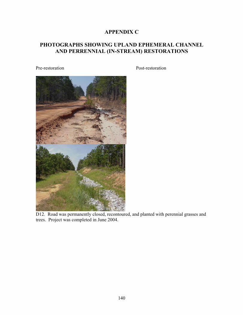
140

APPENDIX C

PHOTOGRAPHS SHOWING UPLAND EPHEMERAL CHANNEL AND PERRENNIAL (IN-STREAM) RESTORATIONS

Pre-restoration Post-restoration

D12. Road was permanently closed, recontoured, and planted with perennial grasses and trees. Project was completed in June 2004.

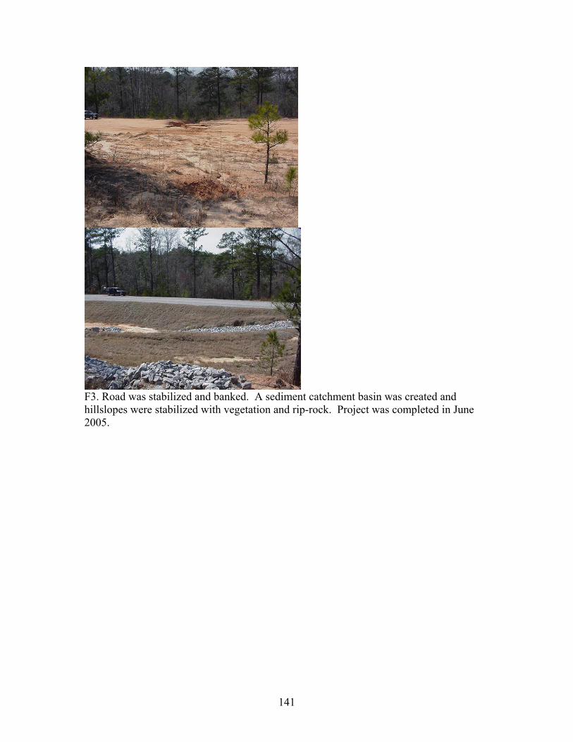
141

F3. Road was stabilized and banked. A sediment catchment basin was created and hillslopes were stabilized with vegetation and rip-rock. Project was completed in June 2005.

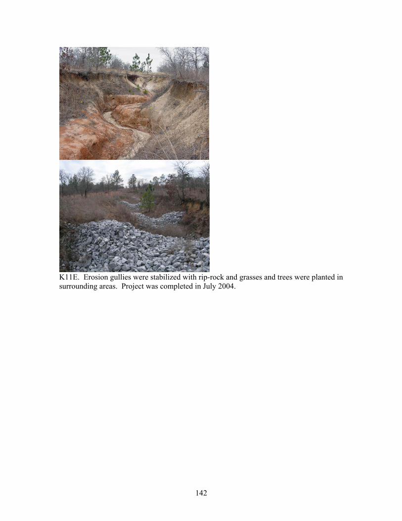
142

K11E. Erosion gullies were stabilized with rip-rock and grasses and trees were planted in surrounding areas. Project was completed in July 2004.

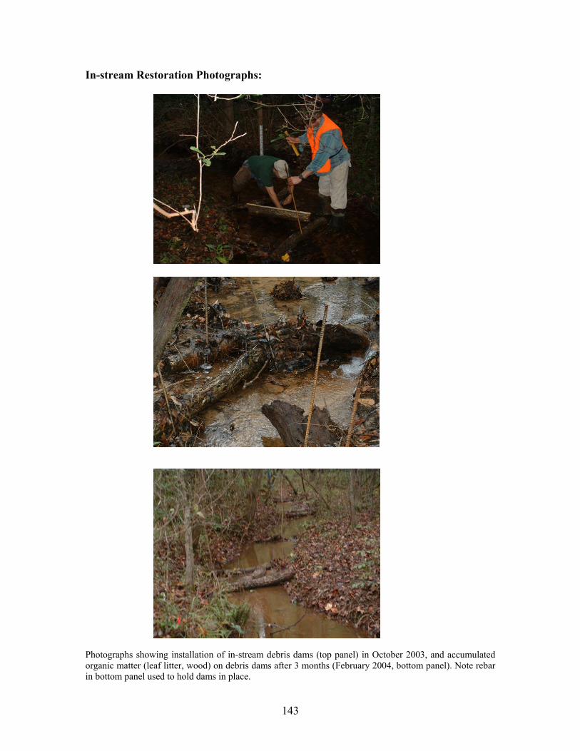
143

In-stream Restoration Photographs:

Photographs showing installation of in-stream debris dams (top panel) in October 2003, and accumulated organic matter (leaf litter, wood) on debris dams after 3 months (February 2004, bottom panel). Note rebar in bottom panel used to hold dams in place.

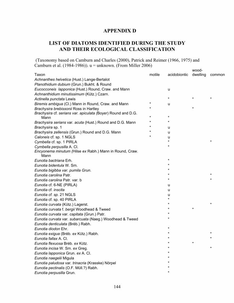
144

APPENDIX D

LIST OF DIATOMS IDENTIFIED DURING THE STUDY AND THEIR ECOLOGICAL CLASSIFICATION

(Taxonomy based on Camburn and Charles (2000), Patrick and Reimer (1966, 1975) and Camburn et al. (1984-1986)). u = unknown. (From Miller 2006)

Taxon motile acidobiontic wood-dwelling common

Achnanthes helvetica (Hust.) Lange-Bertalot Planothidium dubium (Grun.) Bukht. & Round Eucocconeis lapponica (Hust.) Round, Craw. and Mann u Achnanthidium minutissimum (Kütz.) Czarn. Actinella punctata Lewis * * * Biremis ambigua (Cl.) Mann in Round, Craw. and Mann * u Brachysira brebissonii Ross in Hartley * * Brachysira cf. serians var. apiculata (Boyer) Round and D.G.

Mann * * Brachysira serians var. acuta (Hust.) Round and D.G. Mann * * Brachysira sp. 1 * u Brachysira zellensis (Grun.) Round and D.G. Mann * u Caloneis cf. sp. 1 NGLS * u Cymbella cf. sp. 1 PIRLA * * Cymbella perpusilla A. Cl. * Encyonema minutum (Hilse ex Rabh.) Mann in Round, Craw.

Mann Eunotia bactriana Erh. * Eunotia bidentula W. Sm. * Eunotia bigibba var. pumila Grun. * Eunotia carolina Patr. * * Eunotia carolina Patr. var. b * * Eunotia cf. 6-NE (PIRLA) u Eunotia cf. inscita u Eunotia cf. sp. 21 NGLS u Eunotia cf. sp. 40 PIRLA * Eunotia curvata (Kϋtz.) Lagerst. * * Eunotia curvata f. bergii Woodhead & Tweed * * Eunotia curvata var. capitata (Grun.) Patr. * Eunotia curvata var. subarcuata (Naeg.) Woodhead & Tweed * Eunotia denticulata (Bréb.) Rabh. Eunotia diodon Ehr. * Eunotia exigua (Bréb. ex Kϋtz.) Rabh. * * Eunotia fallax A. Cl. * * Eunotia flexuosa Bréb. ex Kϋtz. * * Eunotia incisa W. Sm. ex Greg. * * Eunotia lapponica Grun. ex A. Cl. * Eunotia naegelii Migula * Eunotia paludosa var. trinacria (Krasske) Nörpel * Eunotia pectinalis (O.F. Mϋll.?) Rabh. * Eunotia perpusilla Grun. *

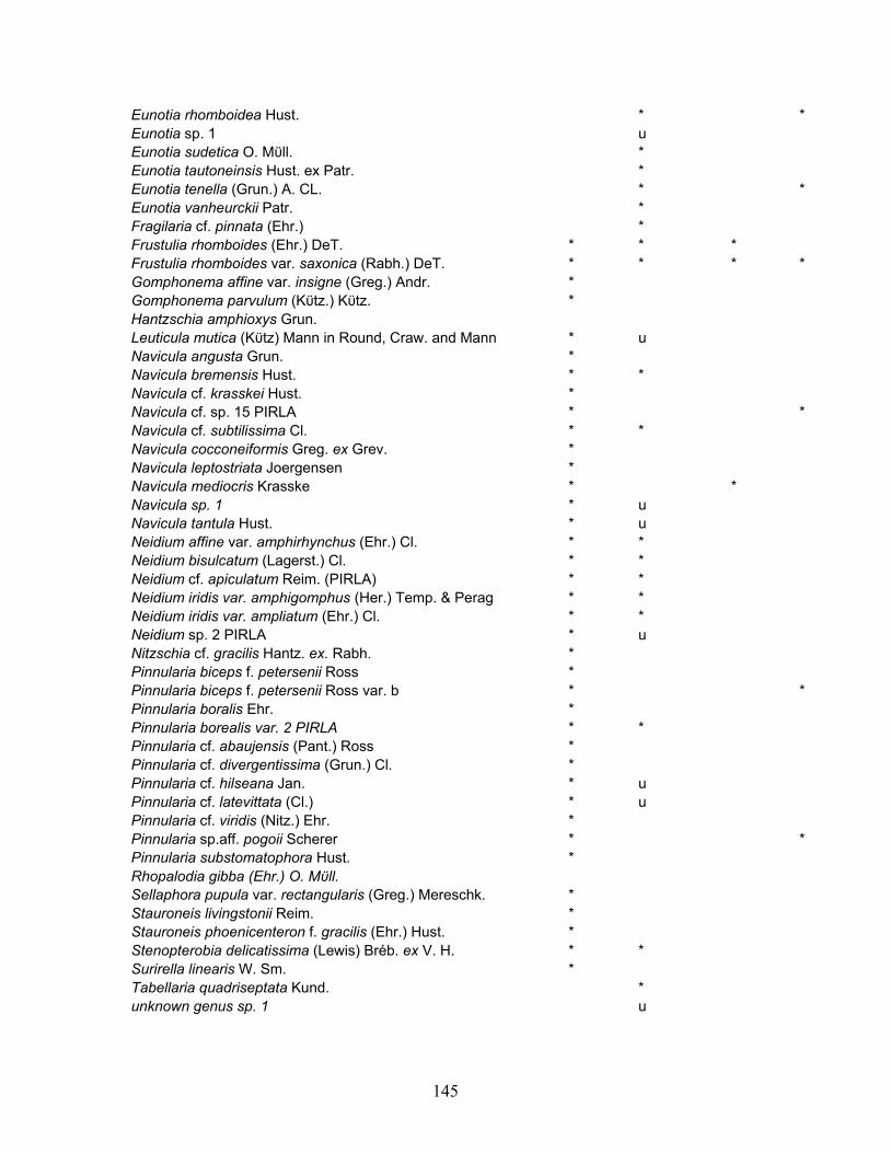
145

Eunotia rhomboidea Hust. * * Eunotia sp. 1 u Eunotia sudetica O. Mϋll. * Eunotia tautoneinsis Hust. ex Patr. * Eunotia tenella (Grun.) A. CL. * * Eunotia vanheurckii Patr. * Fragilaria cf. pinnata (Ehr.) * Frustulia rhomboides (Ehr.) DeT. * * * Frustulia rhomboides var. saxonica (Rabh.) DeT. * * * * Gomphonema affine var. insigne (Greg.) Andr. * Gomphonema parvulum (Kϋtz.) Kϋtz. * Hantzschia amphioxys Grun. Leuticula mutica (Kϋtz) Mann in Round, Craw. and Mann * u Navicula angusta Grun. * Navicula bremensis Hust. * * Navicula cf. krasskei Hust. * Navicula cf. sp. 15 PIRLA * * Navicula cf. subtilissima Cl. * * Navicula cocconeiformis Greg. ex Grev. * Navicula leptostriata Joergensen * Navicula mediocris Krasske * * Navicula sp. 1 * u Navicula tantula Hust. * u Neidium affine var. amphirhynchus (Ehr.) Cl. * * Neidium bisulcatum (Lagerst.) Cl. * * Neidium cf. apiculatum Reim. (PIRLA) * * Neidium iridis var. amphigomphus (Her.) Temp. & Perag * * Neidium iridis var. ampliatum (Ehr.) Cl. * * Neidium sp. 2 PIRLA * u Nitzschia cf. gracilis Hantz. ex. Rabh. * Pinnularia biceps f. petersenii Ross * Pinnularia biceps f. petersenii Ross var. b * * Pinnularia boralis Ehr. * Pinnularia borealis var. 2 PIRLA * * Pinnularia cf. abaujensis (Pant.) Ross * Pinnularia cf. divergentissima (Grun.) Cl. * Pinnularia cf. hilseana Jan. * u Pinnularia cf. latevittata (Cl.) * u Pinnularia cf. viridis (Nitz.) Ehr. * Pinnularia sp.aff. pogoii Scherer * * Pinnularia substomatophora Hust. * Rhopalodia gibba (Ehr.) O. Mϋll. Sellaphora pupula var. rectangularis (Greg.) Mereschk. * Stauroneis livingstonii Reim. * Stauroneis phoenicenteron f. gracilis (Ehr.) Hust. * Stenopterobia delicatissima (Lewis) Bréb. ex V. H. * * Surirella linearis W. Sm. * Tabellaria quadriseptata Kund. * unknown genus sp. 1 u

146