Richard Maliwatu Cape of University

A new connectivity strategy forWireless Mesh Networks using

Dynamic Spectrum Access

Richard Maliwatu

A dissertation submitted in partial fulfillment

of the requirements for the degree of

Doctor of Philosophy

Department of Computer Science

Faculty of Science

University of Cape Town

December 22, 2020

Supervised by:

Dr. David Johnson

Dr. Melissa Densmore

Copyright ©2020 Richard Maliwatu

Univers

ity of

Cap

e Tow

n

The copyright of this thesis vests in the author. No quotation from it or information derived from it is to be published without full acknowledgement of the source. The thesis is to be used for private study or non-commercial research purposes only.

Published by the University of Cape Town (UCT) in terms of the non-exclusive license granted to UCT by the author.

Univers

ity of

Cap

e Tow

n

Declaration

I, Richard Maliwatu, confirm that the work presented in this dissertation is my own

in both concept and execution. Where information has been derived from other

sources, I confirm that this has been indicated in the work.

December 22, 2020

ii

Abstract

The introduction of Dynamic Spectrum Access (DSA) marked an important junc-

ture in the evolution of wireless networks. DSA is a spectrum assignment paradigm

where devices are able to make real-time adjustment to their spectrum usage and

adapt to changes in their spectral environment to meet performance objectives. DSA

allows spectrum to be used more efficiently and may be considered as a viable ap-

proach to the ever increasing demand for spectrum in urban areas and the need for

coverage extension to unconnected communities. While DSA can be applied to any

spectrum band, the initial focus has been in the Ultra-High Frequency (UHF) band

traditionally used for television broadcast because the band is lightly occupied and

also happens to be ideal spectrum for sparsely populated rural areas. Wireless ac-

cess in general is said to offer the most hope in extending connectivity to rural and

unconnected peri-urban communities. Wireless Mesh Networks (WMN) in particu-

lar offer several attractive characteristics such as multi-hopping, ad-hoc networking,

capabilities of self-organising and self-healing, hence the focus on WMNs. Moti-

vated by the desire to leverage DSA for mesh networking, this research revisits the

aspect of connectivity in WMNs with DSA. The advantages of DSA when com-

bined with mesh networking not only build on the benefits, but also creates addi-

tional challenges. The study seeks to address the connectivity challenge across three

key dimensions, namely network formation, link metric and multi-link utilisation.

To start with, one of the conundrums faced in WMNs with DSA is that the cur-

rent 802.11s mesh standard provides limited support for DSA, while DSA related

standards such as 802.22 provide limited support for mesh networking. This gap

in standardisation complicates the integration of DSA in WMNs as several issues

iii

are left outside the scope of the applicable standard. This dissertation highlights the

inadequacy of the current MAC protocol in ensuring TVWS regulation compliance

in multi-hop environments and proposes a logical link MAC sub-layer procedure to

fill the gap. A network is considered compliant in this context if each node operates

on a channel that it is allowed to use as determined for example, by the spectrum

database. Using a combination of prototypical experiments, simulation and numer-

ical analysis, it is shown that the proposed protocol ensures network formation is

accomplished in a manner that is compliant with TVWS regulation.

Having tackled the compliance problem at the mesh formation level, the next

logical step was to explore performance improvement avenues. Considering the

importance of routing in WMNs, the study evaluates link characterisation to de-

termine suitable metric for routing purposes. Along this dimension, the research

makes two main contributions. Firstly, A-link-metric (Augmented Link Metric) ap-

proach for WMN with DSA is proposed. A-link-metric reinforces existing metrics

to factor in characteristics of a DSA channel, which is essential to improve the rout-

ing protocol’s ranking of links for optimal path selection. Secondly, in response

to the question of “which one is the suitable metric?”, the Dynamic Path Metric

Selection (DPMeS) concept is introduced. The principal idea is to mechanise the

routing protocol such that it assesses the network via a distributed probing mech-

anism and dynamically binds the routing metric. Using DPMeS, a routing metric

is selected to match the network type and prevailing conditions, which is vital as

each routing metric thrives or recedes in performance depending on the scenario.

DPMeS is aimed at unifying the years worth of prior studies on routing metrics in

WMNs. Simulation results indicate that A-link-metric achieves up to 83.4 % and

34.6 % performance improvement in terms of throughput and end-to-end delay re-

spectively compared to the corresponding base metric (i.e. non-augmented variant).

With DPMeS, the routing protocol is expected to yield better performance consis-

tently compared to the fixed metric approach whose performance fluctuates amid

changes in network setup and conditions.

By and large, DSA-enabled WMN nodes will require access to some fixed

iv

spectrum to fall back on when opportunistic spectrum is unavailable. In the absence

of fully functional integrated-chip cognitive radios to enable DSA, the immediate

feasible solution for the interim is single hardware platforms fitted with multiple

transceivers. This configuration results in multi-band multi-radio node capability

that lends itself to a variety of link options in terms of transmit/receive radio func-

tionality. The dissertation reports on the experimental performance evaluation of

radios operating in the 5 GHz and UHF-TVWS bands for hybrid back-haul links. It

is found that individual radios perform differently depending on the operating pa-

rameter settings, namely channel, channel-width and transmission power subject to

prevailing environmental (both spectral and topographical) conditions. When ag-

gregated, if the radios’ data-rates are approximately equal, there is a throughput and

round-trip time performance improvement of 44.5 - 61.8 % and 7.5 - 41.9 % respec-

tively. For hybrid links comprising radios with significantly unequal data-rates, this

study proposes an adaptive round-robin (ARR) based algorithm for efficient multi-

link utilisation. Numerical analysis indicate that ARR provides 75 % throughput

improvement. These results indicate that network optimisation overall requires both

time and frequency division duplexing. Based on the experimental test results, this

dissertation presents a three-layered routing framework for multi-link utilisation.

The top layer represents the nodes’ logical interface to the WMN while the bot-

tom layer corresponds to the underlying physical wireless network interface cards

(WNIC). The middle layer is an abstract and reductive representation of the pos-

sible and available transmission, and reception options between node pairs, which

depends on the number and type of WNICs. Drawing on the experimental results

and insight gained, the study builds criteria towards a mechanism for auto selection

of the optimal link option.

Overall, this study is anticipated to serve as a springboard to stimulate the

adoption and integration of DSA in WMNs, and further development in multi-link

utilisation strategies to increase capacity. Ultimately, it is hoped that this contribu-

tion will collectively contribute effort towards attaining the global goal of extending

connectivity to the unconnected.

v

Dedication

To Mom (aka “Mama”), and the memory of Dad. You always placed mwasumba

mano kusukulu as high on the agenda as can be, an instruction time hasn’t touched.

You are the secret master-minders of my PhD journey.

vi

Acknowledgements

There would not have been much of this PhD if it had not been for my supervisors

Dr. David L. Johnson (aka “Dr. DJ”) and Dr. Melissa Densmore who shouldered so

much in the line of admin and constantly kept their hand on the wheel to keep the

boat of my thesis on course, and yet their only reward is me succeeding. I take my

hat off.

I would also like to thank my technical adviser Dr. Albert A. Lysko for all

his advice. Dr. Lysko’s input sharpened the scientific rigour of my work starting

from the research proposal stage of my PhD [...] and along the way enriched my

RF knowledge and terminology use.

My other load of gratitude goes to the Net4d research group crew: Augustine

Takyi, Magdeline Lamola, Amreesh Phokeer, Senka Hadzic, Natasha Zlobinsky,

Hafeni Mthoko and all the ICT4D lab mates <a long list>. I’m thankful for the

helpful comments and discussions, and most importantly for creating a convivial

atmosphere, which saved me trips to the Psychologist’s office.

To my brothers and sisters Harriet, Eddie, Charity, Barbara, Jane and Martin: I

have covered some distance literally and metaphorically. Truth is, I would not have

journeyed as far as I have if it had not been for your encouragement and support

rendered from day one. To Jade: thank you for loving me is my favourite song.

Last but by no means the least, I’m indebted to Hasso Platnner Institute for the

financial support, the Centre of Excellence (CoE) for financial supplements and the

Computer Science Department for thesis fuel supplies among other things. By the

way, “thesis fuel” is a super-technical term for coffee.

Above everything, it’s all by God’s grace.

vii

Biography

The author hails from Zambia, in a rural community called Mporokoso where both

his parents served as teachers at the time. He spent a tiny part of his childhood

in Mporokoso, but as he grew up, he moved to other parts of the country and be-

yond. Between 2001 - 2003, in an attempt to jump-start a career in IT, he read for

his CompTIA Network+, Cisco Certified Network Associate (CCNA), Microsoft

Certified Systems Engineer (MCSE) at North Carolina State University/Computer

Training Unit in Raleigh, North Carolina. Two years later, he pursued the Bache-

lor of Science degree in Computer Science at the Copperbelt University in Kitwe,

Zambia. In 2012 he graduated with Bachelor of Science Honours specialising in

Information Technology at the University of Cape Town. In 2014 he obtained the

Master of Science in Computer Science degree from the University of Cape Town.

His earlier industry certifications tipped him towards the networking side of things

and this has continued to influence his research agenda to this day. But despite all

these credentials, he still doesn’t fully understand how his home router works.

Among the tenets held by the author is the view that, it’s near-impossible to

think of something without being able to mentally construct an image of it. To

prove the point, give an opinion on the itaic speelycaptor? [...] exactly the point!

For this reason, he tries as far as possible to use picturesque illustrations to convey

ideas or concepts. A fair amount of this principle is reflected throughout this thesis.

The author is a Christian and currently serving as Deacon and Secretary at

Mowbray Baptist Church. In between “computer sciencing”, he plays acoustic gui-

tar and electric guitar occasionally, practices all-style Karate and does some cook-

ing, but that’s not to say that he’s good at any of that. Contact: rmaliwatu At cs.uct.ac.za

viii

Publications

Some of the concepts, tables and figures in this dissertation were presented in the

following publications:

• Richard Maliwatu, Albert A. Lysko, David L. Johnson, 2018, November.

Experimental propagation modelling without a dedicated transmitter. In

2018 International Workshop on Computing, Electromagnetics, and Machine

Intelligence (CEMi) (pp. 81-82). IEEE.

Contributed towards chapter 7.

• Richard Maliwatu, Natasha Zlobinsky, Magdeline Lamola, Augustine

Takyi, David L. Johnson, and Melissa Densmore, 2018, September. Ex-

perimental analysis of 5 GHz WiFi and UHF-TVWS hybrid Wireless Mesh

Network back-haul links. In International Conference on Cognitive Radio

Oriented Wireless Networks (pp. 3-14). Springer, Cham.


• Richard Maliwatu, Albert Lysko and David Johnson, 2016, November. Ex-

ploring RSSI Dependency on Height in UHF for Throughput Optimisation.

In 2016 International Conference on Advances in Computing and Communi-

cation Engineering (ICACCE) (pp. 7-12). IEEE.


• Richard Maliwatu, Albert Lysko, David Johnson and Senka Hadzic, 2016,

December. A Correlation between RSSI and Height in UHF Band and Com-

parison of Geolocation Spectrum Database View of TVWS with Ground Truth.

ix

In International Conference on e-Infrastructure and e-Services for Developing

Countries (pp. 243-250). Springer, Cham.


• David Johnson, Natasha Zlobinsky, Albert Lysko, Magdeline Lamola, Senka

Hadzic and Richard Maliwatu, 2016, December. Head to Head Battle of TV

White Space and WiFi for Connecting Developing Regions. In International

Conference on e-Infrastructure and e-Services for Developing Countries (pp.

186-195). Springer, Cham.


• Richard Maliwatu, Natasha Zlobinsky, Melissa Densmore and David John-

son, 2016. Work in progress: A Road Map for Wireless Mesh Routing with

DSA. In Proceedings of Southern Africa Telecommunication Networks and

Applications Conference (SATNAC) (pp. 46-47), George, South Africa.

Contributed towards chapter 1 and 6.

x

Contents

Declaration ii

Abstract v

Dedication vi

Acknowledgements vii

Biography viii

Publications x

List of abbreviations xviii

List of figures xxii

List of tables xxiv

1 Introduction 1

1.1 Motivation . . . . . . . . . . . . . . . . . . . . . . . . . . . . . . . 2

1.2 Problem statement . . . . . . . . . . . . . . . . . . . . . . . . . . 5

1.3 Research questions . . . . . . . . . . . . . . . . . . . . . . . . . . 5

1.4 Dissertation overview . . . . . . . . . . . . . . . . . . . . . . . . . 6

1.5 Overview of the research approach . . . . . . . . . . . . . . . . . . 8

1.6 Research contributions . . . . . . . . . . . . . . . . . . . . . . . . 11

1.7 Thesis outline . . . . . . . . . . . . . . . . . . . . . . . . . . . . . 13

xi

2 Background 15

2.1 Wireless mesh networks overview . . . . . . . . . . . . . . . . . . 15

2.1.1 Advantages of WMNs . . . . . . . . . . . . . . . . . . . . 15

2.1.2 Limitations of wireless mesh networks . . . . . . . . . . . . 16

2.2 Standards on WMNs . . . . . . . . . . . . . . . . . . . . . . . . . 17

2.3 Networking with dynamic spectrum access . . . . . . . . . . . . . 17

2.3.1 Benefits of DSA based communication . . . . . . . . . . . 19

2.3.2 DSA regulatory approaches . . . . . . . . . . . . . . . . . 19

2.3.3 Methods of detecting white space and accessing spectrum . 20

2.4 Standards related to DSA . . . . . . . . . . . . . . . . . . . . . . . 22

2.4.1 IEEE 802.22 . . . . . . . . . . . . . . . . . . . . . . . . . 22

2.4.2 IEEE 802.19 . . . . . . . . . . . . . . . . . . . . . . . . . 23

2.4.3 IEEE 802.11af . . . . . . . . . . . . . . . . . . . . . . . . 24

2.4.4 ECMA 392 . . . . . . . . . . . . . . . . . . . . . . . . . . 25

2.4.5 PAWS . . . . . . . . . . . . . . . . . . . . . . . . . . . . . 25

2.5 Peculiarities of mesh-networking with DSA . . . . . . . . . . . . . 26

2.5.1 Standardisation gap . . . . . . . . . . . . . . . . . . . . . . 26

2.5.2 Limitations of the layered approach . . . . . . . . . . . . . 27

2.6 Chapter summary . . . . . . . . . . . . . . . . . . . . . . . . . . . 28

3 Related work 29

3.1 Method . . . . . . . . . . . . . . . . . . . . . . . . . . . . . . . . 29

3.1.1 Sources of literature and search approaches . . . . . . . . . 30

3.2 Lessons learnt and inspiration drawn from related work . . . . . . . 31

3.2.1 PU region avoidance . . . . . . . . . . . . . . . . . . . . . 31

3.2.2 Routing metrics . . . . . . . . . . . . . . . . . . . . . . . . 34

3.2.3 Multi-channel, Multi-radio systems . . . . . . . . . . . . . 38

3.2.4 Routing in Cognitive Radio Networks . . . . . . . . . . . . 39

3.3 Summary of gaps in related work . . . . . . . . . . . . . . . . . . . 44

xii

4 Towards DSA for TVWS regulation compliant WMN 47

4.1 Problem description . . . . . . . . . . . . . . . . . . . . . . . . . . 47

4.1.1 Existing MAC protocols for DSA enabled nodes . . . . . . 51

4.2 Keeping the TVWS WMN regulation compliant . . . . . . . . . . . 51

4.2.1 Traditional network formation . . . . . . . . . . . . . . . . 54

4.2.2 Proposed network formation to comply with regulation . . . 55

4.3 Formalisation . . . . . . . . . . . . . . . . . . . . . . . . . . . . . 65

4.4 Evaluation of the proposed solution . . . . . . . . . . . . . . . . . 69

4.4.1 Delimiters of the study . . . . . . . . . . . . . . . . . . . . 69

4.4.2 Simulation description . . . . . . . . . . . . . . . . . . . . 70

4.4.3 Correctness of the procedure . . . . . . . . . . . . . . . . . 71

4.4.4 Time to complete mesh formation . . . . . . . . . . . . . . 76

4.4.5 Adapting to changes in inband channel availability . . . . . 82

4.4.6 Limitations of the solution . . . . . . . . . . . . . . . . . . 83

4.5 Discussion . . . . . . . . . . . . . . . . . . . . . . . . . . . . . . . 84

4.6 Chapter summary and future work . . . . . . . . . . . . . . . . . . 86

5 A-link-metric 88

5.1 Notes on metric composition guidelines . . . . . . . . . . . . . . . 89

5.2 Why do we need another routing metric? . . . . . . . . . . . . . . . 91

5.2.1 Variable channel settings . . . . . . . . . . . . . . . . . . . 92

5.2.2 Spectrum availability . . . . . . . . . . . . . . . . . . . . . 93

5.2.3 Interference and link asymmetry . . . . . . . . . . . . . . . 94

5.2.4 Wider frequency range . . . . . . . . . . . . . . . . . . . . 94

5.3 Design philosophy . . . . . . . . . . . . . . . . . . . . . . . . . . 96

5.3.1 Path metric calculation . . . . . . . . . . . . . . . . . . . . 97

5.3.2 Reward and penalty parameter data . . . . . . . . . . . . . 97

5.3.3 Choice of scaling constants . . . . . . . . . . . . . . . . . 99

5.3.4 A case for cross-layering . . . . . . . . . . . . . . . . . . . 99

5.3.5 Link metric selection . . . . . . . . . . . . . . . . . . . . . 100

5.3.6 DPMeS formalisation . . . . . . . . . . . . . . . . . . . . 102

xiii

5.4 Performance evaluation . . . . . . . . . . . . . . . . . . . . . . . . 104

5.4.1 PHY layer modelling . . . . . . . . . . . . . . . . . . . . . 105

5.4.2 Routing protocol description . . . . . . . . . . . . . . . . . 105

5.4.3 Simulation scenarios and setup description . . . . . . . . . 105

5.5 Discussion of findings . . . . . . . . . . . . . . . . . . . . . . . . . 107

5.5.1 Scalability . . . . . . . . . . . . . . . . . . . . . . . . . . 109

5.5.2 Implication of the findings . . . . . . . . . . . . . . . . . . 110

5.5.3 Limitations of the study . . . . . . . . . . . . . . . . . . . 110


6 Characterisation of 5 GHz WiFi and UHF-TVWS hybrid links 113

6.1 Envisaged application scenario . . . . . . . . . . . . . . . . . . . . 116

6.2 Problem description and formalisation . . . . . . . . . . . . . . . . 117

6.2.1 Single point-to-point . . . . . . . . . . . . . . . . . . . . . 119

6.2.2 Point-to-multi-point . . . . . . . . . . . . . . . . . . . . . 120

6.2.3 Multi-point-to-multi-point . . . . . . . . . . . . . . . . . . 121

6.3 Hybrid-link utilisation model . . . . . . . . . . . . . . . . . . . . . 121

6.3.1 Virtual interface . . . . . . . . . . . . . . . . . . . . . . . 121

6.3.2 Link permutation . . . . . . . . . . . . . . . . . . . . . . . 121

6.3.3 Multi-link policy and algorithms . . . . . . . . . . . . . . . 126

6.3.4 Physical interface . . . . . . . . . . . . . . . . . . . . . . . 127

6.4 Experimental evaluation . . . . . . . . . . . . . . . . . . . . . . . 127

6.5 Results and discussion . . . . . . . . . . . . . . . . . . . . . . . . 130

6.5.1 Indoor performance . . . . . . . . . . . . . . . . . . . . . . 130

6.5.2 Outdoor performance: clear line-of-sight . . . . . . . . . . 132

6.5.3 Outdoor performance: near line-of-sight . . . . . . . . . . . 133

6.5.4 Vertical vs horizontal polarization . . . . . . . . . . . . . . 137

6.5.5 Contextualizing performance results . . . . . . . . . . . . . 137

6.5.6 Multi-link performance . . . . . . . . . . . . . . . . . . . . 137

6.6 Towards a mechanism/scheme for auto-selection . . . . . . . . . . . 141

6.6.1 Discussion on what constitutes an optimal configuration . . 144

xiv


7 Other deployment considerations 146

7.1 Experimental setup . . . . . . . . . . . . . . . . . . . . . . . . . . 147

7.1.1 Selecting reference transmitter . . . . . . . . . . . . . . . . 150

7.1.2 Calculating RSSI on a channel . . . . . . . . . . . . . . . . 150

7.2 Findings and discussion . . . . . . . . . . . . . . . . . . . . . . . . 151

7.2.1 Height influence . . . . . . . . . . . . . . . . . . . . . . . 151

7.2.2 GLSD limitations . . . . . . . . . . . . . . . . . . . . . . . 153

7.2.3 Tuning the model . . . . . . . . . . . . . . . . . . . . . . . 155

7.2.4 Other field experiences . . . . . . . . . . . . . . . . . . . . 157


8 Conclusion 159

8.1 Recapitulation of the research questions . . . . . . . . . . . . . . . 160

8.1.1 How should a self-configuring TVWS network stay com-

pliant in a multi-hop environment? . . . . . . . . . . . . . . 160

8.1.2 What characteristics of a DSA channel should be factored

into a link metric for optimal route selection in WMN with

DSA? . . . . . . . . . . . . . . . . . . . . . . . . . . . . . 161

8.1.3 On what basis should the WMN nodes select single-I/O op-

erating radio, aggregate or split links? . . . . . . . . . . . . 162

8.2 What made this study different? . . . . . . . . . . . . . . . . . . . 163

8.3 Summary of results and contributions . . . . . . . . . . . . . . . . 164

8.3.1 Regulation compliant TVWS mesh network formation . . . 164

8.3.2 Link metric . . . . . . . . . . . . . . . . . . . . . . . . . . 165

8.3.3 Multi-radio utilisation . . . . . . . . . . . . . . . . . . . . 165

8.4 Limitations of the research . . . . . . . . . . . . . . . . . . . . . . 166

8.5 Opportunities for future work . . . . . . . . . . . . . . . . . . . . . 167

8.5.1 Extension of the study to other spectrum bands . . . . . . . 167

xv

8.5.2 Extend coverage without incurring a decrease in effective

throughput . . . . . . . . . . . . . . . . . . . . . . . . . . 168

8.5.3 Enhancing GLSD performance . . . . . . . . . . . . . . . . 169

8.5.4 Exploration of other spectrum opportunities . . . . . . . . . 170

8.6 Concluding remarks . . . . . . . . . . . . . . . . . . . . . . . . . . 171

References 173

Appendices 196

A 802.11s key features -an overview 196

A.1 Neighbour discovery and topology formation . . . . . . . . . . . . 197

A.2 Mesh Peering Management finite state machine . . . . . . . . . . . 200

A.3 Beaconing and synchronisation . . . . . . . . . . . . . . . . . . . . 203

A.4 Channel switching . . . . . . . . . . . . . . . . . . . . . . . . . . 203

B Scalability analysis using USL 205

C Link conflict graph 209

C.1 Overview . . . . . . . . . . . . . . . . . . . . . . . . . . . . . . . 209

C.2 Modelling the effects of wireless interference . . . . . . . . . . . . 211

C.3 Estimating path capacity . . . . . . . . . . . . . . . . . . . . . . . 212

C.3.1 Assumptions . . . . . . . . . . . . . . . . . . . . . . . . . 213

C.3.2 Path throughput . . . . . . . . . . . . . . . . . . . . . . . . 221

C.3.3 Illustrative results, implication and concluding remarks . . . 223

D Code snippets 225

D.1 Auto-channel setting for ad-hoc mode . . . . . . . . . . . . . . . . 225

D.1.1 Current limitations and possible future enhancements . . . . 231

D.2 NS-3 simulation . . . . . . . . . . . . . . . . . . . . . . . . . . . . 231

D.2.1 Disable/enable passive/active scanning mode . . . . . . . . 231

D.2.2 Set/check operating channel . . . . . . . . . . . . . . . . . 232

D.2.3 Encode/decode packets . . . . . . . . . . . . . . . . . . . . 235

xvi

E Miscellaneous detail 237

E.1 GLSD query and response messages . . . . . . . . . . . . . . . . . 237

F Reflection 239

F.1 Reasoning by analogy . . . . . . . . . . . . . . . . . . . . . . . . . 239

F.1.1 The price tag . . . . . . . . . . . . . . . . . . . . . . . . . 240

F.1.2 The delivery guy: inspiration for routing . . . . . . . . . . 241

F.2 Design first, model later vs model first, design later . . . . . . . . . 244

F.3 Progression of ideas . . . . . . . . . . . . . . . . . . . . . . . . . . 245

F.4 Two-ply vs single-ply toilet paper . . . . . . . . . . . . . . . . . . 246

F.5 Master key, or maybe not . . . . . . . . . . . . . . . . . . . . . . . 246

F.6 In the end, everything is virtual . . . . . . . . . . . . . . . . . . . . 247

xvii

List of abbreviations

ARR - Adaptive Round-Robin

BRR - Basic Round-Robin

CCC - Common Control Channel

DSA - Dynamic Spectrum Access

FSA - Fixed Spectrum Access

ICT - Information and Communication Technology

IEEE -Institute of Electrical and Electronics Engineers

IP - Internet Protocol

LOS - Line of Sight

NIC - Network Interface card

OSI - Open Systems Interconnection

POP - Point of Presence

QoS - Quality of Service

RF - Radio Frequency

TVWS - Television White Space

UHF - Ultra High Frequency

VSAT - Very Small Aperture Terminal

WCN - Wireless Community Network

WiFi - Wireless Fidelity

WMN - Wireless Mesh Network

WRAN - Wireless Regional Area Network

WSD - White Space Device

xviii

List of Figures

1.1 The world’s offline population . . . . . . . . . . . . . . . . . . . . 3

1.2 The ever increasing demand for improved performance . . . . . . . 4

1.3 Dissertation overview. . . . . . . . . . . . . . . . . . . . . . . . . 7

1.4 Overview of the research approach employed during the study. . . . 10

2.1 Using masts for point-to-multipoint coverage extension. . . . . . . . 16

2.2 Coexistence system architecture. . . . . . . . . . . . . . . . . . . . 24

2.3 Basic network architectures. . . . . . . . . . . . . . . . . . . . . . 25

2.4 Cross-layer thinking with reference to the Open System Intercon-

nect model. . . . . . . . . . . . . . . . . . . . . . . . . . . . . . . 27

3.1 Using the theory of three concentric circles to determine the rele-

vance of work. . . . . . . . . . . . . . . . . . . . . . . . . . . . . 31

4.1 Free space path loss (FSPL) vs distance for a 470 MHz signal. . . . 48

4.2 Route on optimal path based on spatial/temporal spectrum availability. 49

4.3 Comply with regulation first, then optimise performance . . . . . . 50

4.4 Realising a WMN compliant with TVWS regulation. . . . . . . . . 56

4.5 Three-way handshake for regulation-compliant network formation

and operating channel unanimisation. . . . . . . . . . . . . . . . . 57

4.6 Making WMN regulation compliant amid fragmented spectrum. . . 61

4.7 DSA-enabled mesh node state machine. . . . . . . . . . . . . . . . 67

4.8 Best case covergence time. . . . . . . . . . . . . . . . . . . . . . . 78

4.9 Worst case covergence time. . . . . . . . . . . . . . . . . . . . . . 79

4.10 Simple example to explain topology effect on convergence speed. . 81

xix

4.11 Radio frequency spectrum scan over a 24 hour period . . . . . . . . 83

5.1 Networking evolution and progression of routing protocols and

metrics. . . . . . . . . . . . . . . . . . . . . . . . . . . . . . . . . 92

5.2 Multiple forward and reverse throughput samples taken over a pe-

riod of time on both UHF-TVWS and 5 GHz WiFi radios. . . . . . 95

5.3 Path metric calculation between nodes X and Y. . . . . . . . . . . . 98

5.4 Scaling constants . . . . . . . . . . . . . . . . . . . . . . . . . . . 99

5.5 Traffic patterns induced by routing decisions impacts the channel

performance. . . . . . . . . . . . . . . . . . . . . . . . . . . . . . 100

5.6 Dynamic link metric setting. Refer to Table 3.2 (page 37) for the

concept matrix serving as a guide for dynamic path metric selection

from known/pre-determined sets of metrics for a given scenario. . . 101

5.7 Conceptual depiction of network classification based on node and

link characteristics. . . . . . . . . . . . . . . . . . . . . . . . . . . 104

5.8 Overview of network scenarios used to compare base metric with

augmented metric. . . . . . . . . . . . . . . . . . . . . . . . . . . . 106

5.9 Performance results. . . . . . . . . . . . . . . . . . . . . . . . . . 108

6.1 Spectrum requirements by region. . . . . . . . . . . . . . . . . . . 114

6.2 Densely spaced high-frequency APs combined with judiciously

placed low-frequency APs . . . . . . . . . . . . . . . . . . . . . . 115

6.3 Envisaged application scenario using a combination of WiFi and

TVWS to extend broadband connectivity . . . . . . . . . . . . . . . 116

6.4 Possible link options when using 5 GHz WiFi and UHF-TVWS hy-

brid links . . . . . . . . . . . . . . . . . . . . . . . . . . . . . . . 117

6.5 Transmission options for a basic point-to-multi-point link. . . . . . 120

6.6 Multi-link utilisation framework. . . . . . . . . . . . . . . . . . . . 122

6.7 Link permutation analysis. . . . . . . . . . . . . . . . . . . . . . . 123

6.8 Radio link splitting opportunity. . . . . . . . . . . . . . . . . . . . 124

xx

6.9 Link asymmetry caused by primary transmitters and other sources

of strong RF signals . . . . . . . . . . . . . . . . . . . . . . . . . . 125

6.10 Outdoor setup . . . . . . . . . . . . . . . . . . . . . . . . . . . . . 128

6.11 Indoor setup. . . . . . . . . . . . . . . . . . . . . . . . . . . . . . 130

6.12 Throughput vs txpower at a short distance on a 20 MHz channel. A

similar trend was observed for 10 MHz and 5 MHz channels. . . . . 131

6.13 Aerial view of outdoor measurement sites. . . . . . . . . . . . . . 132

6.14 Performance of 5 GHz WiFi and UHF-TVWS links for different

txpower and channel width combinations. . . . . . . . . . . . . . . 133

6.15 Setup of near line-of-sight link obstructed by tree. . . . . . . . . . . 134

6.16 Throughput of UHF-TVWS and 5 GHz WiFi over a link obstructed

by trees. . . . . . . . . . . . . . . . . . . . . . . . . . . . . . . . . 135

6.17 Link obstructed by a building structure . . . . . . . . . . . . . . . . 136

6.18 Throughput of UHF-TVWS over a link obstructed by a building

structure . . . . . . . . . . . . . . . . . . . . . . . . . . . . . . . . 136

6.19 Performance of individual radios, aggregate and split link from the

indoor setup . . . . . . . . . . . . . . . . . . . . . . . . . . . . . . 138

6.20 Basic round-robin vs adaptive round-robin . . . . . . . . . . . . . . 140

7.1 Setup of antenna covered with a low permittivity radome mounted

on boom lifter used to perform measurements. . . . . . . . . . . . 148

7.2 RSSI thresholds for 802.11g radio data rates. . . . . . . . . . . . . 151

7.3 RSSI dependency on height and achievable throughput (Mbps) for

a range of RSSI thresholds. . . . . . . . . . . . . . . . . . . . . . . 152

7.4 Possible options when using 5 GHz WiFi and UHF-TVWS hybrid

links. . . . . . . . . . . . . . . . . . . . . . . . . . . . . . . . . . 154

7.5 Comparing the predicted signal strength with the measured value . . 157

A.1 Ad-hoc mode does not support multi-hopping by default. . . . . . . 197

A.2 Protocol interaction in the MPM framework. . . . . . . . . . . . . . 199

A.3 Finite state machine of the mesh peering management protocol. . . . 201

xxi

B.1 Scalability analysis in terms of convergence. . . . . . . . . . . . . . 208

C.1 Single radio single channel five-node chain topology and its associ-

ated 1-hop and 2-hop conflict graphs. . . . . . . . . . . . . . . . . . 210

C.2 Two-radio two-channel five-node chain topology and its associated

single-hop conflict graph. . . . . . . . . . . . . . . . . . . . . . . 210

C.3 Basic two-node setup. . . . . . . . . . . . . . . . . . . . . . . . . 214

C.4 Basic three-node V-topology setup. . . . . . . . . . . . . . . . . . . 215

C.5 Six-node chain topology. . . . . . . . . . . . . . . . . . . . . . . . 216

C.6 Three by three grid layout. . . . . . . . . . . . . . . . . . . . . . . 219

F.1 Reasoning by analogy . . . . . . . . . . . . . . . . . . . . . . . . . 240

xxii

List of Tables

2.1 Potential benefits of DSA for urban and rural community connec-

tivity requirements. . . . . . . . . . . . . . . . . . . . . . . . . . . 18

3.1 Routing protocols supporting multiple routing metrics. . . . . . . . 35

3.2 Concept matrix of routing metrics. A dash (- ) is used to indicate

missing detail. . . . . . . . . . . . . . . . . . . . . . . . . . . . . 37

4.1 Features of a TVWS WMN with respect to regulatory compliance. . 52

4.2 Regulatory requirements. . . . . . . . . . . . . . . . . . . . . . . . 53

4.3 Using individual nodes’ channel ordering to determine network-

wide operating channel. . . . . . . . . . . . . . . . . . . . . . . . . 64

4.4 Description of terms used in Figure 4.7. . . . . . . . . . . . . . . . 68

4.5 Simulation settings . . . . . . . . . . . . . . . . . . . . . . . . . . 71

4.6 Channel availability at selected locations. . . . . . . . . . . . . . . 72

4.7 GLSD query/response size and minimum link speed required . . . . 74

4.8 Execution completion times observed on the Mikrotik RB433 based

node . . . . . . . . . . . . . . . . . . . . . . . . . . . . . . . . . . 82

5.1 Ideal properties of composite routing metrics . . . . . . . . . . . . 90

5.2 Sensitivity of routing metrics to factors affecting link throughput. . 92

5.3 Example definition of the augmentation factor . . . . . . . . . . . . 97

5.4 Simulation configuration . . . . . . . . . . . . . . . . . . . . . . . 107

6.1 Node specifications. . . . . . . . . . . . . . . . . . . . . . . . . . . 129

6.2 Rule-based link option selection criteria for multi-radio enabled nodes142

xxiii

7.1 Throughput optimisation techniques commonly applied at different

layers of the OSI reference model. . . . . . . . . . . . . . . . . . . 147

7.2 RMSE of propagation modelling. . . . . . . . . . . . . . . . . . . . 155

B.1 Network convergence . . . . . . . . . . . . . . . . . . . . . . . . . 206

B.2 Modelling non-linearity . . . . . . . . . . . . . . . . . . . . . . . . 207

B.3 USL computed parameters . . . . . . . . . . . . . . . . . . . . . . 207

C.1 Conflict matrix for setup 1 . . . . . . . . . . . . . . . . . . . . . . 214



C.4 Conflict matrix for setup 4 single-I/O link option . . . . . . . . . . 220

C.5 Conflict matrix for setup 4 aggregate link option . . . . . . . . . . . 221

C.6 Summary of setup . . . . . . . . . . . . . . . . . . . . . . . . . . . 222

C.7 Estimated link/path capacity for different hybrid link configurations 223

E.1 GLSD query. . . . . . . . . . . . . . . . . . . . . . . . . . . . . . 237

E.2 GLSD response. . . . . . . . . . . . . . . . . . . . . . . . . . . . . 238

E.3 Parameter example size . . . . . . . . . . . . . . . . . . . . . . . . 238

xxiv

Chapter 1

Introduction

Access to Information and Communication Technology (ICT) infrastructure has the

potential to enable provision of services in sectors such as education, health and

governance regardless of the distance to the community. ICTs have a bearing on

many other areas, hence unsurprisingly the United Nations working group on sus-

tainable development goals explicitly lists increasing access to ICT, and providing

universal and affordable access to Internet in least developed countries by 2020.

Although access to cellular phones and mobile broadband has been growing at a

rapid rate in recent years, mobile penetration has not solved the issue of affordable

access. Among the available options for the last mile, the roll-out cost of copper-

wired links is comparatively high and the infrastructure may be targeted by thieves

because of the high value of copper. Fibre optic networks are an alternative, but

for low-income communities the capital required to set it up renders it less viable

for extension beyond the point of presence (POP) and in some cases the terrain

makes the implementation of cabled infrastructure impractical. VSAT is capable of

covering remote areas but the required initial and recurring costs are prohibitively

high. Therefore, open spectrum wireless access technology offers the most hope in

extending connectivity to rural areas [1, 2].

In response to the need for network access, wireless community networks

(WCN) such as TakNet [3], Zenzeleni [4], LinkNet [5] et al. have become a com-

mon trend as confirmed by the Global Information Society Watch 2018 [6] based on

reports from 43 different countries on community networks. WCNs are established

1

for purposes of resource sharing, which may encompass Internet connectivity and

are typically community owned, decentralised and tend to expand organically.

It is in this WCN broad context that this dissertation is situated. Critical as-

pects of WCNs include selecting the right wireless technology suited to the terrain

and population density, and using routing techniques to find the best routes through

a heterogeneous set of radios and link technologies. Looking back at when wire-

less IP-networking emerged, it was quickly discovered that routing protocols ported

from the wired environment were not suitable for use in a wireless environment due

to peculiarities of the wireless media. Similarly, the emergence of Dynamic Spec-

trum Access (DSA) based WMN marks an important juncture in the development

of networking that necessitates a re-adaptation of the routing solutions to suit the

DSA environment. This research revisits the problem of routing in WMN to address

some of the challenges and explore the opportunities that DSA brings.

1.1 Motivation

Firstly, improvement in broadband Internet capacity and access is identified among

key actions required in establishing a strategic economic infrastructure in South

Africa’s National Development plan [7]. Therefore, the high concentration of pop-

ulation in Africa and parts of Asia that is still offline according to the International

Telecommunication Union (ITU) 2016 report calls for concern. From the ITU re-

port in Figure 1.1, it is clear that more effort is needed towards robust network

performance and leveraging spectrum availability within the confines of regulation

for extension of connectivity to rural and under-served populations.

Secondly, the ever increasing demand for high throughput implies that there

is always a constant need for added improvement in network performance. It can

be said that network technology develops over time with the aim of meeting user

requirements. In line with that, the theory of disruptive technology [8] seems to

suggest that a technological solution develops to a point where it meets user require-

ments as illustrated in Figure 1.2a. However, the theory of disruptive technology’s

assertion completely ignores the evolution of user requirements. For example, a

2

study on the implication on performance and usage of Internet bandwidth upgrade

revealed that performance improvement follows soon after an upgrade, but usage

evolves over a short period of time thereby resulting in deterioration of network per-

formance [9]. These findings though based on a specific case hints at the fact that

wireless routing techniques that have been developed meet user Quality of Service

(QoS) requirements but only for a brief period of time. Akin to Parkinson’s Law

[10], in the longer term, user requirements change and keep ahead of the network

performance curve as illustrated in Figure 1.2b. Thus the question of how much

network performance improvement suffices to meet user requirements and keep the

solution curve ahead of QoS requirements permanently is still an open problem.

Europe20.9%

Africa74.9%

Percentage of individuals not using the Internet

The Americas35.0%

CIS33.4%

Asia & Pacific58.1%

Arab States58.4%

0-25

26-50

51-75

76-100

Figure 1.1: The world’s offline population. Source: International TelecommunicationUnion (ITU), November 2018 ICT data.1

The current shift to 5G promises massive bandwidths, however the 2018 ITU

report [11] and other analyses point out that the current cost of deploying a 5G

network makes it viable only in densely populated urban areas, which have always

been the most attractive for operators. With the operators seeing little incentive

to invest in 5G for rural and suburban communities, the GSMA 2018 report [12]

1https://www.itu.int/en/ITU-D/Statistics/Documents/statistics/2018/ITU Key 2005-2018 ICT data with%20LDCs rev27Nov2018.xls

3

predicts that low-income regions such as sub-Saharan Africa for example, will be

last in seeing the launch of 5G. The GSMA forecast further predicts that by the year

2025, 5G may only account for around 2.6% of the total connection base in these

areas. Based on these analyses it is thought that 5G deployments may inadvertently

contribute towards widening the digital divide rather than bridging it.

Time

Development

(a) Ideally

Time

Dev

elop

men

t

Networktechnology

Performance requirements

(b) Reality

Figure 1.2: The intention behind network performance improvement is to develop a so-lution to a point where user requirements are met. In reality network perfor-mance improvements develop, meet user requirements for a short moment but,the QoS demands soon change and keeps ahead of the solution curve2. Someexample causes of performance requirements stepping include the emergenceof technologies such as virtual reality, home video streaming, etc.

2Inspired by a sketch used by Gary Marsden to illustrate the answer to the question, “is the elec-tronic industry in a mature state?” The response to the question considered Clayton M. Christensen’sideas on disruptive technology [8].

4

1.2 Problem statementWhile urban areas are faced with an apparent spectrum crunch, rural areas gener-

ally have a combination of poor connectivity and abundant spectrum. In this regard,

adopting DSA potentially offers several connectivity benefits for both rural and ur-

ban region connectivity requirements ( see section 2.3). However, there is little

support for DSA in the current WMN related standards such as 802.11s whilst stan-

dards pertaining to DSA such as 802.22 offer limited support for mesh networking.

Consequently, attempting to combine the benefits of optimal spectrum utilisation

that DSA brings and the self-organising properties of mesh networking leads to

several confounding challenges at different layers of the network protocol stack.

With the objective of building on the advantages of WMNs with DSA, the aim

of this work is to design a network that makes optimal use of available spectrum and

routes traffic over optimal paths. The network must require very little maintenance,

auto-configure itself, be low cost and comply with applicable DSA regulation.

1.3 Research questionsThis research attempted to address the problem by revisiting the challenge of rout-

ing in WMNs using DSA. The challenge was tackled across three key dimensions,

namely network formation, link metric and multi-link utilisation. The network for-

mation part encompasses measures to address regulation compliance concerns as

well as routing based on spatial spectrum availability. The following three ques-

tions were posed to guide the research agenda:

(i) How should a self-configuring TVWS network stay compliant in a multi-hop

environment?

Prior attempts at cognitive routing focus on the ‘temporal’ aspect of the spec-

trum opportunity and assume a uniform spectrum map for all the nodes. En-

visaging deployment scenarios with several primary transmitters and possibly

other secondary users under different administrative domains spread across

the deployment area, this study addressed the problem of network formation

and topology management amid temporal lack of common optimal channels

5

among WMN nodes. The study leveraged spatial spectrum reuse with the

aim of using a non-interfering optimal common channel between source and

destination node pairs (see chapter 4).

(ii) What characteristics of a DSA channel should be factored into a link metric

for optimal route selection in WMNs with DSA?

Given multi-hop path options comprising multi-radios using different fre-

quency bands and variable channel widths, a metric to characterise links for

optimal path selection is required.

(iii) On what basis should WMN nodes select single-I/O, aggregate or split the

operating radio link?

The term single-I/O is being used to refer to a link using a single-radio

transceiver. A split link in this context is defined as a configuration where

a node uses one radio for sending packets and the other for receiving. An

aggregate link refers to two or more radios combined to form a single logi-

cal link. The performance of radios operating in different spectrum bands or

channels may vary. As a matter of fact, aggregating or splitting could improve

or degrade performance depending on the type of radio and nature of the en-

vironment. Therefore, a framework and criteria are needed for determining

when to use a single-I/O radio, and when to aggregate or split the link.

1.4 Dissertation overviewTo start with, it was critical to get a firm understanding of the DSA regulatory frame-

work applicable to this research’s jurisdiction and identify the opportunities as well

as challenges. The other significant prerequisite was to ascertain white space avail-

ability in the area as this forms the bedrock. Having considered the WMN spec-

trum requirements under the lens of regulatory framework constraints, the research

agenda prioritised DSA regulation compliance concerns in a multi-hop environment

identified through a careful analysis. The study attempted to address the compliance

issue at the MAC layer and once that was accomplished, the next logical step was

6

to explore network performance improvement avenues. The study identified gaps

in the current state-of-the-art and explored opportunities to enhance performance

at the physical layer and network layer in what might be viewed as a middle-cut

approach with respect to the MAC layer. Figure 1.3 gives the broad layout of this

dissertation. Given the opportunities and challenges informed by careful analysis,

the research firstly addressed DSA regulation compliance concerns in a multi-hop

environment at the MAC layer, and secondly tackled the much needed throughput

enhancements at the physical layer and network layer. The ordering of tasks is a de-

liberate reflection of the principle that compliance rather than optimisation should

be of foremost concern.

Needs assessment Understand

regulation, opportunities and challenges

Spectrum analysis Ascertain UHF

white space spectrum availability

Enhance performance Reinforced link metrics Adaptive metric

selection

MAC layer

Physical layer

Network layer

Address compliance concerns Compliant mesh

formation Address possible

common channel shortage

Enhance performance Implement UHF-TVWS/5

GHz hybrid links Fine-tune propagation

modelling Abstract physical layer

complexity for optimal hybrid link utilisation

Figure 1.3: Dissertation overview.

7

1.5 Overview of the research approach

The main aim of the research was to contribute effort towards tackling the routing

challenges arising from combining mesh networking with DSA. Guided by the re-

search questions highlighted in the previous section, the study consisted of three

main parts. An experimental approach was used to conduct the research and quanti-

tative data was used to address the research questions. The South African regulator

- Independent Communications Authority of South Africa (ICASA) have published

TVWS regulation that specifies 470-694 MHz as the radio frequency range for white

space devices (WSD) under the constraints of interference protection requirements.

Thus this research started off with a preliminary spectrum analysis of the 470-694

MHz frequency range. The purpose of the spectrum analysis was twofold: (i) as-

certain availability of TVWS in the area; and (ii) begin to understand the unique

characteristics of UHF signal propagation such as degree and extent of obstacle

penetration capabilities and the effect of factors such as antenna height. This was

followed by an exercise of building actual WMN node prototypes that were later

used for experimentation throughout the study.

The spectrum analysis results were used to understand white space availability

and the extent of variations in spectrum usage over time. This informed the assump-

tions made in answering the first research question and influenced design choices

such as appropriate spectrum sensing and route update intervals. A prototype was

developed as proof of concept. The routing technique was evaluated by comparing

performance with existing solutions using standard network performance metrics as

criteria. This was done firstly using the test-bed implementation for validation and

latterly using simulated mesh nodes for scalability. Figure 1.4 summarises the major

research steps taken. The three parts of this research collectively aim at supporting

two broad functions of a WMN protocol, which are maintaining connectivity and

choosing paths with optimum throughput between any packet source/destination

pairs.

To tackle the second research question, quantitative data was collected to iden-

tify factors influencing link performance and determine the extent to which each

8

of the factors affect the link. The study used the concept of weighted exponential

sum approach not to formulate an optimisation problem, but instead as a method of

estimating the achievable throughput along a given multi-hop path. The resulting

performance objective-based routing metric was implemented in NS-3 network sim-

ulation environment. The evaluation process involved implementing the new metric

used for estimating link and path quality, and comparing performance with existing

routing metrics under different network topologies.

With reference to the overall research approach shown in Figure 1.4, building

on existing elements within the simulation framework, some of the aspects that

had to be modelled in answering the first and second research questions included

spectrum availability, the extent and degree of RF interference on wireless links,

position of nodes in a mesh network and so forth. The simulation on the other hand

was conducted to mimic mesh network processes with a specific focus on formation

and routing tasks.

To address the third research question, measurements were conducted to inves-

tigate link performance using different multi-radio settings, namely operating chan-

nel, transmission power, channel width and antenna polarisation. Performance was

measured under different environmental variables namely, trees/vegetation, build-

ing structures and landscape. These environmental factors are known to impinge

on the Fresnel zone and subsequently affect the Radio Frequency (RF) signal prop-

agation. The WMN router consisted of 5 GHz WiFi and UHF-TVWS radios. A

detailed description of the prototype is given in chapter 6.

The measurement process involved setting up the nodes on two ends of a site in

different environments. With the help of a measurement script, throughput, delay,

packet loss and other values of interest were recorded for various combinations of

operating parameters. A custom measurement script was developed for this purpose

that executed control commands between node pairs using a dedicated control link

established using 3G modems. With a dedicated control link in place, the data

collection process had minimal impact on the experiments conducted on the 5 GHz

WiFi and UHF-TVWS links.

9

simulation

Thesis

Data collection & analysis

Results

Realistic experiment scenarios

Literature survey

Pick research topic &formulate research questions

Solution design

no

yes

Refine the modelling

Data consistent with testbed

measurements?

Outdoor testbed measurements to

evaluate real world performance

Indoor testbed to establish baseline

performance

Preliminary field measurements to

establish spectrum availability and usage

pattern

Refine solution

Figure 1.4: Overview of the research approach employed during the study.

10

1.6 Research contributionsWhilst addressing the research questions, this study makes the following four con-

tributions pertaining to the design and implementation of WMNs with DSA:

• DSA regulation compliant WMN formation, routing based on spectrum

availability

This study identified a critical gap in the readiness of the current WMN MAC

layer implementation to ensure DSA regulation compliance from device boot-

up to complete network formation. The multi-hop nature and ad-hoc char-

acteristics poses significant challenges in network formation when WMNs

apply DSA. This research extends the existing 802.11s mesh standard by in-

troducing a logical link MAC sub-layer procedure aimed at ensuring regula-

tion compliance from device start-up through the complete multi-hop network

formation process. Furthermore, envisioning a wireless network deployment

scenario spanning a large geographical area with non-contiguous white space,

when there is no clean operating channel available globally, a scheme of rout-

ing is developed that allows the mesh routing protocol to route traffic based

on spectrum availability. Radio virtualisation was applied amid constraints of

single-radio nodes to mitigate the problem of temporal lack of common clean

channel and avoid interfering with primary transmissions. In addition to as-

serting the technical feasibility of realising a WMN compliant with TVWS

regulation, an enquiry into the nodes’ mechanism for correcting the potential

risk of interfering with incumbents based on the current protocol to access

white space (PAWS) culminated in two key findings. Firstly, there is a min-

imum Internet link speed that is required for mesh nodes to transact with

the GLSD within a period of time that is small enough to minimise the im-

pact of interference during that process. The Regulator can impose this as

an additional requirement for TVWS in multi-hop environments. Secondly,

GLSD protocols should be designed with this requirement in mind, for exam-

ple by prioritising mandatory parameters and allowing the optional features

to be turned on/off to reduce overhead especially for GLSD queries using

11

low-speed Internet connections. Refer to chapter 4 for more details.

• Augmented link metric

The research highlights the inadequacies in existing link metrics that are

based on implicit measurements. ‘implicit’ in the sense that they use higher

layer parameters to deduce link layer status. The study provides a general

framework and guidelines for reinforcing existing metrics to factor in char-

acteristic of a DSA channel. To test the concept, the augmented link metric

incorporates raw data obtainable from wireless network cards to infer link

performance. The augmented link metric improves the routing protocol’s

ranking of links for optimal path selection by prioritising high throughput

links based on raw data from the radios, which gives a more accurate mea-

sure of link quality as opposed to applying network layer parameters to infer

link performance.

• Dynamic Path metric selection

Routing protocols perform differently using different metrics in different sce-

narios. Building upon the well known fact that when it comes to link metrics,

there is no “one size fits all”, this dissertation introduces Dynamic Path Met-

ric Selection (DPMeS). DPMeS extends the scope of the routing protocol to

encompass mechanisms and criteria for determining the suitable routing met-

ric for the network. DPMeS is an attempt to unify this and other prior studies

on different link metrics. DPMeS is driven by a pre-routing phase component

introduced in the routing process. Instead of configuring the routing proto-

col with a fixed routing metric, the pre-routing phase is initially a start-up

process and latterly a periodic process that the routing protocol carries out to

assess the network and auto-configure a suitable routing metric to use. Refer

to chapter 5, section 5.3.5 for a more detailed description.

• Multi-link utilisation framework, criteria and technique

Given multi-radio enabled nodes, this dissertation presents a framework for

optimal multi-link routing for WMN hybrid back-haul links. A three-tiered

12

framework that makes a distinction between possible link configurations and

multi-link utilisation policies is proposed. This decomposition allows for the

different link configurations to be coupled with an appropriate policy to meet

the different performance objectives. In addition, an adaptive round-robin

(ARR) based aggregation technique is presented to enhance efficiency of ag-

gregate links with non-uniform data-rates.

The notion of ARR in itself is not a new concept. The principle has been ap-

plied over scheduling problems in different forms across several areas such as

blocking of packets in the access point’s buffer [13], uplink bandwidth alloca-

tion for mobile WiMAX [14], load balancing of distributed web servers [15],

CPU scheduling [16] et al. However, to the extent of the author’s knowledge,

this is the first time the principle and technique is being applied for efficient

utilisation of multi-rate hybrid links.

While the study focused on 5 GHz WiFi and UHF-TVWS based hybrid links,

the proposed framework is technology-agnostic and thus can be applied to

any multi-link capable nodes regardless of the underlying operating spectrum

band. Background details of the multi-link utilisation framework are pre-

sented in chapter 6 with particular emphasis in sections 6.3 and 6.5.6.

1.7 Thesis outlineThe rest of this thesis is organised as follows:

Chapter 2 presents the underpinning background theory used throughout this

study. More specifically, the chapter gives an overview of WMNs and outlines

the routing problem in WMN. The chapter also introduces DSA and discusses

regulatory and incumbent protection approaches.

Chapter 3 reviews the current state-of-the-art and existing literature most

closely related to this study. The chapter ends off with a summary of gaps

identified in related work and highlights elements that set this research apart

from related work.

13

Chapter 4 highlights the challenge of meeting TVWS regulation compli-

ance in a multi-hop environment comprising long distance links. The chapter

presents the proposed mesh formation protocol aimed at achieving TVWS

regulation compliance right from the network formation phase.

Chapter 5 focuses on the link metric aspect of routing in WMNs using DSA.

The chapter pinpoints inadequacies in existing link metrics and discusses the

proposed approach.

Chapter 6 motivates the need for a performance prediction model. The chap-

ter presents the design and evaluation of the proposed framework for optimal

multi-link utilisation.

Chapter 7 explores the dependency of received signal strength indicator on

height for throughput optimisation and discusses additional considerations

relevant to the deployment of TVWS-based networks.

Chapter 8 recapitulates the research problem and summarises the key findings

and contributions of this research. The chapter concludes with a discussion

of limitations of the study and future research directions.

14

Chapter 2

Background

2.1 Wireless mesh networks overviewDue to low up-front costs and easy expansion associated with wireless mesh net-

working, the technology presents a viable alternative solution towards effort aimed

at extending connectivity to rural and under-served areas. A wireless mesh network

(WMN) comprises mesh clients and mesh routers. Mesh routers take part in the

relaying of network traffic and play the role of gateway or repeater. Mesh clients

on the other hand refers to end-user devices such as laptops and phones that con-

nect to the mesh network for services via Ethernet or mesh access points. Mesh

network architectures may be placed in three generic categories namely infrastruc-

ture, client and hybrid WMN. WMNs may further be classified as point-to-point,

point-to-multi-point, and multi-point-to-multi-point depending on the nature of con-

nectivity.

2.1.1 Advantages of WMNs

Regardless of the type of architecture, the key attractive characteristics that set

WMN apart from other types of networks include multi-hopping, ad-hoc network-

ing and capabilities of self-organising and self-healing, multiple types of network

access and interoperability with other wireless networks [17].

Furthermore, using masts as illustrated using dotted lines in Figure 2.1 to

extend connectivity adds to the infrastructure costs. Secondly, analysis of signal

strength measurements in the UHF band at different heights shows a high correla-

15

tion between signal strength and receiver antenna height. On channels with high

signal strength, the television transmitter signal increases by as much as 2.5 dBm

per 1 m increase in height above the ground [18]. It is expected that the noise floor

will have a stronger negative impact on mesh nodes at high sites especially when

they move ”spectrally” closer to television transmitters [19]. Mesh networking on

the other hand (illustrated with solid lines in Figure 2.1), allows us to lower the ra-

dios, which reduces costs as well as the amount of interference inflicted by primary

transmitters but, still able to extend connectivity using multi-hopping.

A

B

Figure 2.1: Using masts for point-to-multipoint coverage extension.

2.1.2 Limitations of wireless mesh networks

Multi-hopping in ad-hoc mode is not enabled by default, it is effected by applying

routing. The ensuing disadvantage is that, it becomes difficult to use dynamic host

configuration protocol (DHCP) when using Internet Protocol version 4 (IPv4). This

is because a DHCP request will not be forwarded across a multi-hop link, and so

IPv4 addresses have to be statically assigned [20], which can be tedious if the WMN

consists of more than a few nodes. Possible workarounds include autoconfiguring

IPv6 addresses from the devices’ MAC address [21].

Furthermore, General Systems Theory (GST) describes the whole as being

16

greater than the sum of its individual parts i.e. 2+2 > 4. For a WMN this synergis-

tic view holds substantially true in terms of coverage extension and fault tolerance,

but not so in the throughput aspect. Effective end-to-end throughput reduces as the

number of hops increases. For example, assuming a uniform transmission rate of

W bits per second at each node, asymptotically the worst and best case throughput

is respectively in the order of

W√n log(n)

and W√n where n is the number of hops [22].

Experimental results show that the TCP throughput under ideal conditions is given

by

Wn0.98 which is significantly less than the theoretical predictions [23].

2.2 Standards on WMNsWMNs are commonly deployed using wireless technology based on IEEE 802.11.

Besides proprietary solutions, WMNs are typically realised by combining the

802.11 MAC protocol with layer 3 ad-hoc routing [20], [24], or layer 2 ad-hoc

routing [25] depending on the architecture and application as mentioned in section

2.1. One notable WMN specific standard is the 802.11s [26], [27]. The 802.11s

standard specifies Independent Basic Service Set (IBSS) mode connection among

mesh nodes and also supports client node connections to the mesh nodes.

2.3 Networking with dynamic spectrum accessMotivated by the increased demand for bandwidth in the license-free frequency

bands and under-utilisation in the licensed bands, numerous proposals [28, 29, 30]

have in recent years been put forward towards opportunistic spectrum access. Op-

portunistic spectrum access also referred to as Dynamic Spectrum Access (DSA)

is a spectrum assignment paradigm where devices are able to make real-time spec-

trum usage adjustments and adapt to changes in their spectral environment to meet

performance objectives. Spectrum is viewed as consisting of three abstract regions,

namely white space, black space and gray space [31], [32], [33].

17

White space is the term used to refer to parts of the licensed spectrum that are

vacant either spatially or temporally i.e. unused in a given geographical location or

unused for an amount of time. When the white space under consideration is unused

television channels around a given region, then it is defined largely in frequency

terms.

Black space refers to the region inside the primary user’s coverage zone such that

the secondary system is able to detect the primary signal and therefore cancel the in-

terference. Black space based communication is where a radio deliberately utilises

the same frequency as the primary transmitter provided an inconsequential amount

of interference is caused. The black space radio meets that requirement by turning

the transmission power down to a sufficiently low level.

Gray space is the region outside the primary user’s coverage area where the sec-

ondary system receives a significant amount of interference, but in principle is not

close enough to cancel the interference from the primary user.

DSA potentially allows unlicensed users access to licensed portions of the

spectrum when not in use by the licensed users. Researchers, industry and ad-

ministrations have blamed the apparent spectrum shortage on inefficient spectrum

resource utilisation associated with Fixed Spectrum Access (FSA) schemes cur-

rently in place. Therefore, DSA may be considered as a viable solution to the ever

increasing demand for spectrum in urban areas and the need for coverage extension

to unconnected areas as summarised in Table 2.1.

Urban RuralTypicalcharacteristics

spectrum crunch, densepopulation

abundant spectrum, sparse popu-lation, poor connectivity

Applicationscenario

MetroNets, IoT last mile connectivity

Ideal spectrumfeatures

high frequencies, shortrange

lower frequencies, long trans-mission range

Potential DSAbenefit

efficient spectrum utili-sation

lower cost of extending connec-tivity by using spectrum on asecondary basis

Table 2.1: Potential benefits of DSA for urban and rural community connectivity require-ments.

18

2.3.1 Benefits of DSA based communication

Internet Protocol (IP) based wireless networks that use DSA have several benefits in

comparison with their FSA counterparts. DSA benefits emanate from the capability

to select spectrum with desired characteristics such as longer transmission range,

better obstacle penetration and minimal interference caused/suffered. The benefits

of DSA based communication can be substantiated by analysing path-loss and the

physics of three basic propagation mechanisms, namely reflection, diffraction, and

scattering characterising the operating spectrum. Studies have shown that wireless

communication using alternative portions of the spectrum offers several improve-

ments over the 2.4/5 GHz bands that WiFi uses. The electromagnetic properties of

waves in the ultra high frequency (UHF) television band for example, have a number

of advantages when used for communication, such as enhanced signal propagation,

which allows for longer transmission range and obstacle penetration [34].

Traditionally, governments through their respective agencies assign national

licenses (usually at a fee) for users to operate in a particular frequency band exclu-

sively. These assignments stay unchanged over the license validity period, typically

5-20 years. The cost of spectrum incurred by service providers is inevitably passed

on to the consumer. Studies have shown that FSA results in inefficient spectrum

utilisation [35, 36, 37]. White space can be found in any frequency band such as

4G (LTE) and Very High Frequency (VHF). However, the current emphasis is on

the UHF television white space (TVWS) because this is where the most significant

white space is found. In addition, TVWS is ideal spectrum for rural connectivity.

2.3.2 DSA regulatory approaches

The three main spectrum sharing approaches are Licensed Shared Access (LSA),

Collective Use of Spectrum (CUS) and hierarchical model [38].

LSA is a regulatory approach where a limited number of users are authorised to

use a frequency band that is already assigned to one or more incumbent users pro-

vided they do so in accordance with the applicable sharing rules agreed upon by the

incumbents and the secondary users. Under LSA, secondary users are given indi-

vidual licences and both secondary LSA licensees and primary users are guaranteed

19

protection from interference.

CUS is a general authorisation where an unlimited number of independent users are

allowed spectrum access in the same range of designated frequencies at the same

time under a set of conditions. Under CUS class of usage, devices are allowed to

use unused spectrum found through the device’s own capability. Unlike LSA, the

number of CUS users is not controlled, which implies QoS depends on the level of

congestion.

Hierarchical model combines the operational principles of LSA and CUS. Similar

to LSA, incumbents are given top priority to access spectrum at any point in time

whereas, secondary licensees are given priority when spectrum is not in use by

the primary user. Under the hierarchical model, there is a general authorisation

similar to CUS when spectrum is not in use by neither primary nor secondary user.

Unlike CUS, the hierarchical model general authorisation applies to the same band

licensed to primary and secondary users. The term light-license is sometimes used

to describe this type of general authorisation. Users may be required to register

with the regulatory authority that might limit the number of authorisations or restrict

registration to particular entities such as tertiary institutions for example.

2.3.3 Methods of detecting white space and accessing spectrum

The methods for identifying white space fall in one of three general categories

namely geolocation spectrum database (GLSD), pilot channel and spectrum sens-

ing used independently or one method combined with another [39].

GLSD involves establishing a regulator-approved central database that a device

queries to get white space spectrum information at the device’s location. There

are two main schemes used for the GLSD to learn about spectrum availability at

a particular location. The first is a data-driven approach that uses spectrum mea-

surements for particular locations. The second is model-driven where spectrum

availability at a given location is computed using radio frequency models [40]. The

data-driven approach has the benefit of determining white space with precision how-

ever, widespread measurements are required, which could take a long time to ac-

complish. In addition, radio frequency spectrum scans have to be re-done whenever

20

new transmitters are added or there are changes in transmission characteristics such

as antenna height, transmission power or location of the primary transmitter. The

model-driven approach is convenient but, the performance in terms of complexity

and accuracy depends on the particular model used. Secondly, the method requires

up-to-date information on primary transmitters.

Spectrum sensing requires the secondary device to continuously monitor its ra-

dio environment to detect the presence of incumbents, and determine the available

channels. Conventionally, spectrum sensing refers to the measurement of the ra-

dio frequency energy on the channel. However, in the context of cognitive radio,

sensing can be broadened to include other dimensions such as code and angle [41].

Sensing techniques fall into one of two main categories, energy detection, and fea-

ture detection based sensing [42]. Energy detection compares the energy detector

output with a noise floor dependent threshold to determine presence of signal on a

given channel. The feature detection method captures spectral signatures such as

cyclostationarity, segment-synch, pilot, etc. depending on the type of signal under

consideration.

Data fusion is a term used to describe an approach that combine GLSD with sens-

ing. Spectrum database information is complemented by sensing to cater for dy-

namic incumbent usage patterns. Sensing could also be used for establishment of

initial connection to the database or to obtain granular information on the available

channels.

Beacons/Pilot channel is a centralised cellular-based implementation where coex-

istence information is shared over a known control channel [43]. A secondary user

may transmit in white space if it receives a beacon signalling availability of a chan-

nel. Oppositely, a secondary user may continue transmission on a given channel

until it receives a beacon declaring the channel unavailable.

Out of these three methods of identifying white space spectrum, GLSD is

widely considered as the immediate viable solution largely because of its centralised

nature, which eases implementation complexities. In addition, the GLSD method

offers guaranteed levels of protection to incumbents. However, the current GLSD

21

implementation is only concerned with protection of primary users and remains ag-

nostic to secondary spectrum usage. Research has shown that the level of tolerable

interference reduces as multiple devices access adjacent channels at the same time

[44], but existing regulation is nonetheless mainly concerned with protection of pri-

mary users and has not stipulated methods of coexistence among multiple secondary

users accessing white space simultaneously [45]. Therefore, more work remains

to be done in developing spectrum etiquette protocols and managing coexistence

among secondary spectrum users.

This research investigated GLSD performance for white space detection and

found that as currently deployed, GLSD alone is inadequate in determining white

space accurately (see section 7.2.2). The GLSD is prone to inaccuracies due to rea-

sons ranging from limitations in propagation modelling to tending lack of up-to-date

primary transmitter information. Furthermore, the GLSD may indicate a particular

channel to be unoccupied based on primary transmitter (e.g. television broadcast)

information, however the channel may be tainted by incumbent signals due to high

decodability threshold [46], and unregistered sources in adjacent channels [47]. In

view of the identified drawbacks of a GLSD when used independently, this disser-

tation recommends a hybrid approach i.e. GLSD coupled with localised spectrum

scans.

2.4 Standards related to DSAIn comparison with fixed transmission medium, white space technology is still in

its infancy. However several standards have already been drafted in alignment with

the white space communication paradigm. The following sections provide a brief

description of standards from the IEEE 802 groups [48], [49], [50], ECMA [51] and

IETF [52] that are closely related to the emergence of white space based communi-

cation.

2.4.1 IEEE 802.22

The IEEE 802.22 standard specification covers the air interface, including the cog-

nitive medium access control layer (MAC) and physical layer (PHY) of point-to-

22

multipoint wireless regional area networks (WRAN) consisting of a fixed base sta-

tion with fixed and portable end user devices operating in the VHF/UHF television

broadcast bands from 54 MHz to 862 MHz. The principal assumption behind IEEE

802.22 is that communication devices share spectrum with primary users and as

such, spectrum availability may vary from time to time and place to place. In ad-

dition to the 54 MHz - 862 MHz range, the spectrum may span 1300 MHz to 1750

MHz, and 2700 MHz to 3700 MHz. These bands may differ from country to coun-

try as they were specified by the FCC for the United States. However, the standard

is intended to align emerging regulations with the current 802.22 technology and

enable interoperability among WRAN products from different vendors.

2.4.2 IEEE 802.19

The IEEE 802.19 standard specifies radio technology independent methods for co-

existence among dissimilar devices or independent networks of devices operating in

television bands. Coexistence has been defined as the ability of multiple spectrum-

dependent devices or networks to operate without harmful interference. Coexis-

tence is viewed as a service rendered by the coexistence system to white space

devices. This system consists of three logical entities that use TCP/IP in all the

exposed interfaces as shown in figure 2.2.

The standard outlines two classes of coexistence algorithms: coexistence dis-

covery and coexistence decision algorithms. Coexistence discovery algorithms are

used by the coexistence discovery and information server (CDIS), and the coexis-

tence manager (CM) to discover white space devices that might interfere with each

other. The CM uses coexistence decision algorithms to reconfigure white space de-

vices to avoid interference. The standard describes several algorithms for each class

but, does not restrict implementation to any particular algorithm. In addition, the

standard does not provide any specificity on the physical implementation. There-

fore, the coexistence functionality may be built into a single device or the role of

logical entities may be enabled in separate devices.

In addition to specifically addressing coexistence among IEEE 802 devices for

effective use of TVWS, the IEEE 802.19 standard is also projected to be useful

23

TVWS database

Coexistence discovery and information server

Coexistence manager 1 Coexistence manager 2

White space devie/network

Scope of IEEE 802.19

Coexistence enabler

Figure 2.2: Coexistence system architecture.

for non IEEE 802 networks as well. Furthermore, though the standard specifies a

TVWS database logical entity, the architecture can be generalised so much so that

the system works with any method of white space detection e.g. sensing, and in

other spectrum bands.

2.4.3 IEEE 802.11af

The IEEE 802.11af standard covers specific requirements for local and metropoli-

tan area networks. It is an amended IEEE 802.11 physical layer (PHY) and medium

access control (MAC) sub-layer enhanced to support operation in TVWS. The

amendment adds a Television Very High Throughput (TVHT) PHY specification

using orthogonal frequency division multiplexing (OFDM) based on the geoloca-

tion database control for TVWS detection and incumbent protection. The standard

defines basic channel units (BCUs), namely 6 MHz, 7 MHz or 8 MHz depending on

the regulatory domain. This implies that two contiguous BCUs provides 12 MHz,

14 MHz or 16 MHz, and four contiguous BCUs would provide 24 MHz, 28 MHz

or 32 MHz. Single BCU transmission mode is mandatory whereas, use of multiple

BCUs is optional.

24

Peer device Master deviceSlave deviceData flow Control flow

Figure 2.3: Basic network architectures.

2.4.4 ECMA 392

The standard specifies a MAC sub-layer and a PHY layer for personal/portable cog-

nitive wireless networks operating in TVWS. Three device modes namely, master,

slave, and peer are defined but, the standard does not support autonomous device

mode transition. In a master-slave configuration, the master coordinates network

formation, channel access, and communication between slave devices as illustrated

in figure 2.3. On the other hand, in a peer-to-peer network, devices use distributed

beaconing and channel reservation to coordinate channel access. A peer-to-peer

network may also be described in this context as ad-hoc, self-organising, and self-

healing. The standard also specifies a MAC client (MUX sub-layer) for higher

protocols and several incumbent protection mechanisms that may be used to meet

regulatory requirements. These mechanisms include protocols for detecting incum-

bents, coordinated channel measurement, dynamic channel selection, and transmit

power control.

2.4.5 PAWS

The Protocol to Access White Space (PAWS) is a standard protocol defined by IETF

to achieve interoperability between devices and databases of spectrum availability.

Spectrum databases store information on spectrum availability and protection rules

based on the guidelines of the regulatory domain. The centralised nature of the

database approach provides two key benefits. Firstly, the approach relieves the de-

25

vice of the complexities associated with spectrum-policy conformance. Secondly,

in the event of a policy change, updates are limited to database thereby simplifying

adoption as opposed to updating numerous devices. PAWS is built on top of HTTP

and Transport Layer Security (TLS) protocol, and allows a device with geolocation

capability to query the database appropriate for the location and obtain spectrum

availability information. The standard defines two types of devices i.e. a master

that uses a URI (dynamically/statically obtained) to interact with the database di-

rectly and a slave that queries the database through the master device.

2.5 Peculiarities of mesh-networking with DSA

The advantages of DSA when combined with mesh networking not only build on

the benefits of WMNs, but also compounds the challenges as well. This section

discusses some of the challenges arising when DSA is applied to mesh networking.

2.5.1 Standardisation gap

To begin with, there are a number of WMN applicable standards, different DSA

regulatory frameworks and several DSA related standards as described in sections

2.2, 2.3.2 and 2.4 respectively. However, at the time of writing this dissertation, a

standard that bridges WMN and DSA requirements is yet to be drafted. For exam-

ple, ICASA’s draft TVWS regulation [53], [54] stipulates that a WSD must query a

GLSD whenever the WSD’s position changes by 100 m or more. This requirement

is befittingly in anticipation of variations in the RF spectrum map potentially aris-

ing with every 100 m shift in location. However, the regulation provides little or no

guidelines on how mesh nodes operating in ad-hoc mode (prospectively placed hun-

dreds of metres apart) ought to access and coordinate spectrum usage. Therefore,

running the WMN on a common optimal and clean DSA channel without interfer-

ing with primary transmissions at one corner of the network remains a significant

challenge. In addition, WMNs with fixed spectrum operate on a set of fixed chan-

nels that remain fairly unchanged over time, whereas it is expected that the state of

a WMN with DSA will be influenced by the activities of primary spectrum users.

26

2.5.2 Limitations of the layered approach

Communication between devices is often described with reference to the layer

model. Protocol designers refer to the layer model as a tool for breaking down

the complex communication process into simpler sub-processes. Using the typical

layer model, individual layers communicate only with neighbouring layers i.e. layer

k only communicates with layer k−1 and layer k+1. The layered approach has the

advantage of breaking down the complex communication problem into a hierarchy

of less-complex layers [55]. Each layer addresses a sub-communication problem

and that allows the development of protocols on one layer to be done independent

of protocols on other layers. This approach has worked well in the more static envi-

ronments. However, in a DSA-based network the sub-problems on one layer do not

interact with other layers in a strict hierarchical fashion, which makes it difficult to

maintain total transparency in the layer functions. For example, when the best path

is defined in terms of channel width availability, the routing protocol may need to

interrogate the MAC layer and possibly the physical layer for such information. In

light of this and other observed limitations of the layered model, there is a general

consensus among researchers [56], [57], [58] that for optimal solutions in multi-

hop wireless networks, it is imperative to adopt a cross-layer design approach. A

cross-layer approach may be defined in two ways: firstly, as the interaction between

non-adjacent layers and secondly, the spanning of a solution across multiple layers

as illustrated in Figure 2.4. Several cross-layer design methodologies in the context

of multi-hop wireless network have been proposed [59], [60], [61]. Characteris-

tics of a DSA-enabled WMN add to the existing motivation for cross-layer design

thinking in multi-hop wireless network environments.

Network layer

Data link layer

Physical layerLayered interaction

Cross-layer interaction

Figure 2.4: Cross-layer thinking with reference to the Open System Interconnect model.

27

2.6 Chapter summaryThe chapter has given an overview of WMNs architectures and described typical

characteristics of mesh networks. The chapter also gave an overview of DSA and

outlined general potential benefits for both rural and urban communities. The dif-

ferent methods of detecting the spectrum opportunity and how these fit into the dif-

ferent DSA regulatory frameworks is also discussed. The chapter also highlighted

the different DSA related standards applicable to different network types. Applying

DSA to WMNs builds on the advantages that WMNs hold, but also compounds the

challenges in the two fields. The chapter ended off with a discussion on some of the

unique challenges faced in WMNs with DSA.

The next chapter presents prior work that is most closely related to this re-

search.

28

Chapter 3

Related work

Wireless mesh networks create multiple possible paths between any sender/receiver

pairs as already mentioned previously in the background chapter. Routing is the pro-

cess of determining the best path between the source node and the target destination

node. Literature abounds with numerous studies on routing in WMNs. This chap-

ter presents a review of the work of other researchers around the thesis topic. The

review was conducted with the intent of gaining insight and a better understanding

of the subject matter. To guide the review and analysis, the following question was

posed: how has the shift toward the DSA paradigm influenced routing in wireless

networks?

3.1 Method

A pool of data comprising resources from online digital libraries as well as the insti-

tutional library were reviewed and analysed. The method draws on a method of sec-

ondary analysis of research by Glass [62] and a systematic qualitative meta-analysis

procedure developed by Ke [63]. Secondary analysis refer to the re-analysis of data

for reasons such as applying better statistical techniques in answering old research

questions or using old data to tackle new questions. Meta-analysis on the other

hand, is the analysis of analyses or the integration of findings from different indi-

vidual studies by analysing a collection of analyses.

29

3.1.1 Sources of literature and search approaches

The studies reviewed were located by manually searching electronic records of

publicly accessible publications that included, but not limited to the following

databases: ACM digital library, Elsevier ScienceDirect, IEEE Xplore, Springer,

UCT Primo and Wiley Science. The search strategy varied depending on the search

tool used. Nevertheless, the general search terms used included “routing in wireless

mesh networks”, “cognitive radio networks”, “wireless network with dynamic spec-

trum access”, “cognitive radio in wireless mesh networks”, “cognitive ad-hoc net-

works”, “next generation wireless networks”, “TVWS mesh network” and “TVWS

network” coupled with backward and forward reference searching 1.

The search results underwent a series of parsing that initially involved a look

at the title and a review of the abstract and entire content depending on the gleaned

degree of relevance to the overarching topic under consideration. The studies con-

sidered in this chapter were selected using a subjective criteria guided by how rele-

vant the source is to this dissertation or aspects of it. The degree of relevance was

determined using the theory of concentric circles as depicted in Figure 3.1. The

concentric circles theory approach was initially postulated by Ernest Burgess to ex-

plain the social structure of urban communities [64]. The method has since then

been widely used in the field of political science to design and analyse foreign pol-

icy [65], [66] among other use cases. The concentric circles theory arranges items

in the scheme of things in terms of concentric circles, which represent a higher or-

der of priority as one moves inward from the outer circle. Extending this way of

conceptualising complex issues, this dissertation applied the concentric circles the-

ory to direct the criteria for inclusion/exclusion of sources. Articles that belonged

to the centremost category were considered most applicable.

1Backward reference searching refers to the process of locating and reviewing the work cited in apublication. Forward reference searching refers to the practice of identifying and examining studiesthat have cited the original work. This helps to understand the evolution and expand knowledge ona given topic.

30

Routing in WMN

+DSA

WMN + DSA

Wireless + DSA

Figure 3.1: Using the theory of three concentric circles to determine the relevance of work.

3.2 Lessons learnt and inspiration drawn from re-

lated workThis dissertation draws from three interrelated fields, namely routing, multi-

channel/multi-radio systems, and cognitive radio networking in the mesh network-

ing context. The following sections discuss findings from studies situated at the

intersection of the aforementioned research directions.

3.2.1 PU region avoidance

One of the (if not the most) critical requirement of any DSA based network is to

avoid causing interference in and around the primary user (PU) region . From a

WMN perspective, the solution needs to carry out two tasks, namely route discov-

ery and route maintenance under the PU protection constraints. These tasks corre-

spond to network formation and topology management functionalities of the mesh

protocol.

Literature is replete with studies such as the enhanced dual diversity cogni-

tive ad hoc routing protocol (E-D2CARP) [67] that identify the problem of network

formation in DSA based ad-hoc networks, but fail to provide a clear solution that

directly addresses regulation compliance in a multi-hop environment from network

formation through the topology management stages. E-D2CARP is an on-demand

protocol that attempts to establish a routing path in a manner that circumvents the

31

PU region(s). The E-D2CARP mechanism involves node(s) that happen to fall in-

side the PU region to set their status to “IN-PU-REGION” and change back to

“OUT-PU-REGION” when there is no PU activity. By so doing, it is expected that

the set of intermediate forwarding nodes between the sender and receiver will ex-

clude the nodes inside the PU region. Besides the drawbacks of on-demand routing

for WMNs, it is not clear from the authors’ report how spectrum status informa-

tion gets communicated among the nodes and how network-wide channel change

transitions are effected, let alone coordinated.

Several other studies [68], [69], [70] attempting to address the problem of net-

work formation in DSA based WMN presuppose devices have access to a common

control channel (CCC). The design of CCC is a separate topic on its own [71], how-

ever with the CCC approach, nodes generally tune to the CCC initially at start-up

and thereafter periodically at predetermined intervals to transmit and listen for con-

trol messages. The CCC approach undoubtedly eases the control and coordination

complexities. However, there is compelling evidence pointing to the fact that the

CCC approach may not be feasible in most deployment scenarios due to lack of

uniformity in the distribution of other transmitters [72].

Given the arguments against the CCC applicability, several other prior related

studies on network formation and topology management in DSA based mesh such

as CogMesh [73], have appropriated cluster based methods. The cluster based ap-

proach groups the nodes in tandem with spectrum availability so much so that the

scope of determining a suitable operating channel is reduced to individual clusters.

The focus of work employing the cluster approach has been on the selection of

cluster heads and optimisation of cluster formation. The major limitation in prior

related work is that they assume a contiguous spectrum map, which is not typically

applicable. On the other hand, work identifying the problem of fragmented spec-

trum [74] address other performance requirements and not the problems associated

with mesh formation.

The other observation made from the literature surveyed is that meeting or im-

proving end-user performance requirements is emphasised while overlooking regu-

32

lation compliance. Prior related works have proposed algorithms that are based on

full network topology information or a priori knowledge of primary users, which is

a valid premise for FSA cases. However, the assumption does not hold for DSA-

based WMNs because of the fragmentation that commonly characterises the spec-

trum space and the ad-hoc nature of WMN connectivity. It can be seen from the

above analysis that there is a general lack of adequate detail on ensuring a regula-

tion compliant network formation process. To back that claim, consider CogMesh

for example, where it is mentioned that if a node fails to find a cluster to join, it ran-

domly chooses a channel and starts a new cluster. The report went on to say that a

cluster-head chooses gateway nodes and interconnects with other cluster-heads. As

can be seen, there is insufficient clarity on how cluster-heads multiple-hops away

get to establish connections. Similar sentiments can be expressed after analysing

the distributed channel assignment algorithms proposed for DSA based WMN [75],

as this also focuses on enhancing performance (assuming the network topology is

formed completely) and does not show how that is achieved in a compliant manner.

Whilst prior related studies have unquestionably not addressed DSA regula-

tion compliance at the mesh formation stage, the mechanisms used at the routing

level to avoid interfering with incumbents can be placed in two generic groupings.

The first approach aims to detect the PU transmission region and attempts to avoid

forwarders (or relay nodes) that fall inside the PU region as explained in the earlier

paragraph. This design assumes that there are other nodes outside the PU region

than can forward packets between the sender and receiver, which may not always

be the case. The second approach is where any node deemed next-best-hop can

forward data traffic, but avoid interfering with the PU by reducing the transmis-

sion power to sufficiently low levels. The assertion is that secondary users can use

the same frequency as primary users provided the secondary users’ power spectral

density is below that of the primary user [76]. The terms overlay and underlay

are sometimes used to respectively refer to spectrum co-existence paradigms where

the secondary user uses vacant channels only and in which the secondary user uses

the same channel as the primary user, but at power levels low enough to eliminate

33

interference with primary users [77].

The obvious drawback of lowering the transmission power is that it is only

viable if the nodes are a short enough distance apart. To explain the relation between

transmission power and transmission distance, consider the famous Friis’ equation

[78]:

Pr = Pt

(λ

4πd

)2

=⇒ d =λ√

Pt

4π√

Pr(3.1)

where Pr = remaining power of the wave at the receiver, Pt = transmission

power of sender, λ = wavelength, d = distance between the receiver and the sender.

It is evident based on equation 3.1 that effective transmission distance reduces when

transmission power is reduced. Therefore, reducing the transmission power as

a method of incumbent protection could potentially result in loss of connectivity

among the nodes at long distances.

3.2.2 Routing metrics

It is worth noting upfront that variations in the way the metric is calculated (e.g

considering efficiency, accuracy, amount of overhead and other aspects) and set-

tings for parameters such as routing packet interval in a given protocol contribute

substantially towards the overall performance. Therefore the performance of rout-

ing metrics (sometimes referred to as path-weight functions) should be analysed

more wholistically.

Routing protocols that support multiple metrics facilitate the evaluation of rout-

ing metrics in that performance variation due to the protocol’s internals is minimised

and differences in performance can more confidently be attributed largely to the

metric properties. Work meeting this criteria includes, Optimized Link State Rout-

ing (OLSR) [79], Dynamic Source Routing (DSR) [80], Multi-Radio Link Quality

Source Routing (MR-LQSR) [81], BatMan-eXperimental Version 6 (BMX6) [82]

as shown in Table 3.1.

A study conducted to compare standard hysteresis and the Expected Trans-

mission Count (ETX) routing metrics using OLSR protocol showed that hysteresis

34

Table 3.1: Routing protocols supporting multiple routing metrics.

Protocol Layer/ Type Supported metricsOLSR 2, link-state Hysteresis, ETX

DSR 2, link-state ETX, hop-count, per-hop RTT

MR-LQSR 2, link-state WCETT, ETX, Hop-count

BMX6 2, distance-vector Vector metric, Transmit quality, ETX, Hop-count

out-performs ETX on all accounts [23]. However, this holds for medium-to-large

size networks (roughly 21 to 49 nodes). For a small to medium size network, ETX

showed better performance.

ETX is generally considered as a superior routing metric to hop-count because

it implicitly captures the hop-count and additionally takes the quality of the links

into account by considering the packet delivery ratio. However, when there is mo-

bility at the sender, hop-count performs better than ETX and Round Trip Time

(RTT) link-quality metrics [80]. Earlier work on WMN routing metrics focused

on accounting for the lossy nature of the wireless medium. As a result, the major

limitation of basic metrics such as ETX and Expected Transmission Time (ETT) is

that they only aim to increase the probability of packet delivery. They do not factor

in interference and are based on the supposition that the links comprise uniform

data-rates.

In response to the limitations of ETX and other basic metrics listed above,

Weighted Cumulative ETT (WCETT) was developed for heterogeneous multi-radio

environments. The report from the study comparing WCETT, ETX and hop-count

implemented in MR-LQSR showed that WCETT provided the best performance

while hop-count yielded the least performance. However, the study did not con-

sider the impact of mobility, which leaves no evidence to support nor refute the

suggestion that hop-count would outperform WCETT in a scenario involving mo-

bility. In addition, there is a paucity of studies to collaborate the authors’ claims

on WCETT. Nonetheless, there is compelling evidence from analytical and simula-

tion studies showing that WCETT itself lacks consideration for inter-flow interfer-

35

ence and isotonicity2 for efficient computation of the minimum weight path. Subse-

quently, in different comparative studies of WCETT with the Metric of Interference

and Channel-switching (MIC), MIC performed superiorly to WCETT [83], [84].

While MIC improves on its predecessor in that it aims to achieve load-balancing

by accounting for inter-flow as well as intra-flow interference interference, it does

not explicitly account for possible variation in data-rates among the different link

options.

The above snippet of collected studies on wireless network routing metrics

albeit narrow, is a sufficient representative sample of the general pattern3 prevailing

in literature regarding the subject of routing metrics for wireless networks. Based

on these and results from other related studies, it can be said with confidence that

each metric typically has a scenario(s) or network condition(s) under which it either

flourishes or fails. Following this line of enquiry, this dissertation drew out the

concept matrix summarised in Table 3.2 to accentuate the core network strands and

associated metrics. This research focused on WMNs comprising static nodes with

no power constraints, however for completeness the concept matrix includes energy

constrained and mobile environments.

While there is sufficient evidence to support the concept of network classes

based on Table 3.2, there is still much to query and explore in the broader task of

choosing the ideal metric. For a start, there is need to develop efficient methods of

detecting network characteristics at the protocol level for purposes of determining

the suitable routing metric. The other thing routing protocol architects need to con-

sider is to develop highly cohesive metric calculation modules and institute loose

coupling between the metric computation functionality and the rest of the routing

mechanism. This will foster the much needed interchange of innovative outputs

from work on routing and routing metrics among different studies. Furthermore,

at present the points of transition for determining factor(s) i.e. where performance

2The isotonicity rule says that the order of the ranking on two paths should be preserved when athird path suffixes or prefixes the paths. See chapter 5 ( Table 5.1) for an expanded definition of thisand other metric properties.

3The observed pattern is that of this metric out-performing that metric, and that metric performingpoorly under a given set of network characteristics or test conditions.

36

Table 3.2: Concept matrix of routing metrics. A dash (- ) is used to indicate missing detail.

NameTarget network/characteristics

Ene

rgy

cons

trai

ned

Mob

ileno

des

Stat

icno

des

Mul

ti-ra

dio

Sing

lera

dio

Uni

form

data

-rat

es

Div

erse

data

-rat

es

Size

S M L

Hop-count X X X - -

Hysteresis X X X

EXT X X X X X

ETT X X X X X -

MIC X X X - -

of one metric begins to deteriorate and the other starts to get better are still only

vaguely clear. All in all, the methods discussed in the previous section may be

described as “best effort” approaches in that the routing protocol chooses a path

deemed optimal for all data traffic.

Other approaches to assign link costs especially in mobile ad-hoc network

(MANET) environments aim to explicitly support QoS for different classes of traf-

fic priorities. One popular approach is to consider the network as an artificial neu-

ral network (ANN) and use link metrics to represent the weights of the ANN [85].

Learning techniques such as genetic algorithms can then be applied to determine the

optimal path based on the optimisation function of the network. For this purpose,

the use of batch based [86] and online based [87] machine learning algorithms to

predict link quality have been proposed in prior related work. In these publications,

the principle of link metric is expressed using the concept of “link quality predic-

tors”. It is apparent that the usefulness of these machine learning based solutions

depend entirely on the accuracy of the underlying prediction model. On one hand,

batch machine learning methods cannot adapt once training is complete and as such

accuracy may decline when the network conditions deviate significantly from the

training data. Online based machine learning algorithms offer a better promise, but

37

on the other hand, at the time of writing this dissertation, integration of online based

machine learning with the routing module is still in its infancy. Therefore, it is un-

clear at this stage if the benefits that ANN promises will materialise because the

aspects encouraging or inhibiting deployment are still unknown. There is a further

dearth of test-bed based implementation and results, which raises concerns about

the practicality of the solutions extending beyond the simulation environment.

There are other metrics highlighted in literature under the “cognitive radio net-

work” umbrella. However, these are yet to be widely implemented and therefore,

the findings are hard to substantiate let alone conduct comparative analyses at this

stage. The other challenge affecting metric exploration is the degree and extent

of coupling between the metric calculation component and the rest of the routing

module. Tight coupling has hindered implementation of metrics in other routing

protocols and eventual evaluation.

3.2.3 Multi-channel, Multi-radio systems

The current IEEE 802.11 based radios are said to be half-duplex i.e. the transmit and

receive operations are not done simultaneously. This limits the network capacity in

that throughput at relay nodes is halved as detailed already in the previous chapter

(section 2.1.2). The capacity and performance of a network can be enhanced by

using multiple channels at the same time. This requires multiple transceivers. Basic

multi-channel capable nodes can be built using the following architectures [88]:

• Multiple hardware platform where two or more single-radio nodes are con-

nected via Ethernet to form one logical multi-radio mesh router.

• Single hardware platform in which a single node has multiple transceivers

fitted.

• Single-chip multi-transceivers where multiple transceivers are integrated into

one wireless chipset on a router.

Enabling multi-radio capability can unarguably improve performance significantly,

however mechanisms are still required to take advantage of the radios. Several rout-

ing protocols and metrics such as MR-LQSR protocol (introduced in section 3.2.2),

38

Weighted Expected End-to-End Delay (WEED) [89] and Generalized Partitioned

Mesh network traffic and interference aware channeL Assignment (G-PaMeLA)

[90] to name but a few, have been proposed for routing in multi-radio scenar-

ios. Other multi-radio network protocols such as Multi-radio Unification Protocol

(MUP) [91] have been implemented at the link layer without modification to the

upper layers. While these protocols are aimed at improving network capacity by

making optimal use of multiple-radios, they are based on static channels and as

such are ill-suited for the DSA environment.

Based on the survey conducted, there is a limited amount of literature on hy-

brid4 back-haul link selection. The work most closely related to this dissertation

worth pointing out are the schemes that have been developed for selecting the ap-

propriate network for specific services given the integration of heterogeneous access

technologies such as WLAN and cellular in 4th generation (4G) communication sys-

tems . The approaches used include Fuzzy logic, Game Theory and mathematical

techniques such as AHP and GRA [92], [93], [94], [95]. While these prior studies

on network selection provide insight into the exploitation of multi-radio enabled

devices for improved performance, the solutions proposed apply mostly to strict

infrastructure based network environments that have some kind of centralised con-

troller such as a base station. New mechanisms are needed to leverage hybrid links

for back-haul WMN connectivity.

3.2.4 Routing in Cognitive Radio Networks

Routing protocols in Cognitive Radio Networks (CRNs) can be classified across

multiple dimensions. Basic categorisation of routing in CRNs classifies the pro-

cess as either single-path or multi-path routing [96]. Single-path routing refers to

single-hop forwarding, whereas multi-path routing is where a network consists of

redundant links between nodes to minimise the impact of interruption caused by

primary user activity. A more comprehensive way uses three major taxonomies that

are based on, extent of spectrum awareness [97], diversity [98], and performance

objective [99].

4Multi-radios utilising different spectrum bands such as a combination of 5 GHz and TVWS.

39

Spectrum awareness based

Spectrum awareness based solutions may further be sub-classified as either full

spectrum knowledge based or partial/local spectrum knowledge based. Spectrum

awareness encompasses cognizance of both spectrum availability as well as spec-

trum quality. Full spectrum knowledge based solutions assume nodes know the full

spectrum occupancy map through the spectrum database or the master node. Thus

spectrum management is done via a centralised entity that may not necessarily be

integrated with the routing process. On the other hand, partial or local spectrum

knowledge based approaches rely on the spectrum information constructed locally

at each node and through distributed protocols, shared among the nodes. Local

spectrum knowledge based solutions are characterised by tight coupling between

spectrum management and routing functionalities.

Several studies [100], [101] have identified the interdependence and shown

that network performance is determined jointly by routing and channel assignment.

For that reason several proposed routing algorithms such as ROSA [102], and Cog-

WMN [103] have adopted the cross-layer [56] design approach to control the inter-

action between the routing and channel selection functionality. In CogWMN, the

wireless mesh network is modelled as an undirected graph. The algorithm combines

the channel allocation method with AODV routing protocol. ROSA and CogWMN

respectively model the multi-hop wireless network as a directed connectivity graph

and undirected graph. A time slotted CCC is assumed for spectrum control and

coordination among the nodes. Both ROSA and CogWMN like many prior related

work assume a pre-existing complete network graph and fail to address the graph

formation part, which is an inevitable part of any WMN setup.

In other efforts, Spectrum Aware Mesh Routing in Cognitive Radio Networks

(SAMER) [104] has been proposed for routing in CRNs. SAMER aims to find

paths with the highest spectrum availability to maximise throughput. SAMER also

attempts to balance the short-term opportunistic gains with associated switching

overhead and the long-term optimality. The major shortcoming of SAMER and in-

deed other related studies is the premised mesh network operation or definition. For

40

example, the authors mention that two communicating nodes have to contend for

spectrum access using a control channel in the unlicensed bands. This view reduces

spectrum requirements to two communicating nodes and completely ignores the

multi-hop nature of mesh networks. The point at issue is that, if two nodes choose

an operating channel that is orthogonal to the one used by its other neighbours,

there is loss of connectivity with the other neighbouring nodes. SAMER could be

a feasible solution if multi-frequency transmission capability among the nodes is

enabled, but that would require a coordination scheme to be implemented, which is

a non-trivial task. To add on, using multiple channels raises the chance of a node

missing the RTS/CTS transaction on one channel while tuned to a different channel.

For this and other reasons, IEEE 802.11 based single-radio mesh nodes have to be

tuned to the same operating channel in order to maintain connectivity and for the

routing protocol to maintain a correct routing table.

The other limitation observed in other related work such as Cognitive Routing

Protocol (CRP) [105], is that they employ a method of ranking the next-best-hop

based on the assumption that all links are symmetric, which is rarely the case in

wireless environment. Therefore, on account of the issues pointed out, a lot remains

to be done in ensuring that joint routing and channel assignment protocols address

the concerns brought out in WMN environments.

Diversity based

Diversity based routing refers to a broad category of routing algorithms that aim to

take advantage of peculiarities of the wireless space such as the inherent broadcast

nature and spatial diversity of the wireless medium. Two of the main approaches

include opportunistic forwarding and network coding.

Opportunistic forwarding itself is a wide class of routing schemes that leverage

transmission opportunities instead of transmitting on a predetermined path. A wire-

less channel is inherently a single broadcast domain and with opportunistic routing,

any node that “hears” the transmission can act as a relay candidate. The maximum

end-to-end throughput with opportunistic forwarding is given by the solution to the

objective function (3.2) given below:

41

maxK

∑k=1

∑lksi∈E

M

∑α=1

µkαsi (3.2)

where E = set of all the wireless links

si = node operating on channel k(1≤ k ≤ K)

µkαi j = transmission rate on each link lk

si

α = (1...M) denotes the times scheduled for concurrent transmissions.Depending on the implementation, the next forwarder(s) can either be specified by

the source or may require coordination among the candidate relay nodes to select

the “best” forwarder. The advantages of opportunistic routing include dynamic

selection of optimal path at the actual time of transmission and the ability (in

principle) to combine multiple weak physical links into a single stronger logical

link.

Network coding is a method of routing where multiple data packets are coded

and delivered through a single transmission. Using this approach, a router can com-

bine packets “over-heard” from different sources and send them out in one trans-

mission. The destination then decodes to obtain the initial set of packets. Network

coding increases efficiency by reducing the required number of transmissions. The

improvement in efficiency realised through network coding is beneficial especially

in multicast scenarios. Furthermore, retransmissions are inevitable due to the lossy

nature of the wireless medium, therefore efficiency in transmission is valuable.

To overcome the limitations of individual diversity-based routing approaches

such as opportunistic forwarding and network coding, an alternative approach is to

appropriate a hybrid solution that combines the two methods in a complementary

manner for added improvements.

Performance objective based

Irrespective of the extent of spectrum awareness and protocol diversity, routing

protocols may be classified based on the performance objective, which could be

link stability, throughput, localisation, energy based or multi-objective and so forth.

Atomic metrics such as delay, hop-count, ETT, ETX, et al. are often combined as

42

shown in equation 3.3 for improved performance trade-off.

minx

F(x) = [F1(x),F2(x), ...,Fn(x)] (3.3)

where F(x) is a vector of performance objective functions Fi(x) and n repre-

sents the number of objective functions or atomic metrics [106].

The optimal routing path is modelled by defining a global utility function M

that is a combination of individual utility functions Mi where 1≤ i≤ n. Combining

atomic metrics to form a global utility function is done using one of four main

common methods namely, weighted exponential sum or product, Lexicographic,

weighted min-max and constraint-based [96].

i Weighted exponential sum sums up the atomic metric exponentially as

shown in equation 3.4 or multiplies as shown in equation 3.5 to form the

global utility function.

M(r) =n

∑i=1

wi[Mi(r)]p (3.4)

where r is the routing path, M(r) is the global performance objective function,

which corresponds to F in equation 3.3, wi > 0 is the weight of atomic metric

i, ∀1 ≤ i ≤ n, p is a constant parameter such that 1 ≤ p ≤ inf. The weight

of the atomic elements w has to be decided, which renders the weighted sum

method subjective depending on the choice of weights.

M(r) =n

∏i=1

[M(r)]wi (3.5)

ii Lexicographic global metric is where atomic metrics are ordered by level of

importance and individual utility functions solved one at a time as shown in

equation 3.7.

minr Mi(r) such that (3.6)

M j(r)≤M j(r∗)+ ε,1≤ j ≤ i−1 (3.7)

43

where M j(r∗) is the optimum found in the jth iteration and ε is a tolerance

parameter.

iii Weighted min-max criteria aims to achieve fairness and balance among the

atomic metrics.

M(r) = max1≤i≤n

wi[Mi(r)−Ci] (3.8)

where Ci for i = 1,2, ...,n are constraints.

iv Constraint-based approach does not weight the atomic metrics unlike the

previously listed methods, but instead, one atomic metric is selected and re-

garded as the principal metric while the other metrics are considered con-

straints as shown below:

maxx

Mi∗(r) (3.9)

Amini ≤Mi(r)≤ Amax

i (3.10)

where i∗ denotes the atomic metric considered as the global metric, Amini and

Amaxi are the other atomic metrics’ constraints.

Overall, individual objectives are often conflicting, which makes the solution

unachievable. In such cases of contradistinction among performance objectives, it

suffices to aim for a pareto-optimal5 solution.

3.3 Summary of gaps in related workSeveral studies have demonstrated the benefits of DSA. The topic of wireless net-

working with DSA has been studied more extensively in the context of cellular

networks compared to the WMN context. The cellular environment possesses sev-

eral characteristics that fundamentally differ from the WMN frame of reference.

Therefore, the implementation of DSA in WMNs is expected to be different as al-

ready alluded to in section 2.5 of the previous chapter. National regulators in several

5The term Pareto-optimal has its roots in the field of economics. It is applied in this context torefer to a solution or set of solutions that cannot be improvement further in one dimension withoutworsening in some other aspect(s) [107].

44

countries including South Africa have recently passed regulation allowing the use

of WSDs in the UHF band. Among the conditions is the requirement for WSDs to

query a GLSD for spectrum availability. There are two possible repercussions to

regulation coming into effect: (i) a number of solutions proposed prior, may be ren-

dered invalid depending on the extent to which assumptions initially premised de-

viate from regulatory requirements; and (ii) the complexities of prior solutions with

the associated overhead resulting from the assumed degree of spectrum dynamic-

ity and the need to balance between the gains and the cost of switching spectrum

may be less justifiable. The rest of this section discusses challenges central to the

implementation of DSA in WMNs that still need to be addressed.

To reiterate, the problem of network formation6 is yet to be addressed. For

example, COMNET [75] proposes an algorithmic framework for frequency shifting.

COMNET focusses on frequency shifting for a given cluster or set of clusters i.e.

grouping of a wireless mesh router with its connected mesh clients. The study

assumes a completely formed WMN in which each node location is known to all

the other nodes. The aspect of coordination among the nodes in a self-organising

mesh network is not clear. This dissertation in chapter 4 addresses the problem of

WMN formation in relation to TVWS regulation compliance.

Furthermore, DSA-based networks are expected to operate on a wider range of

frequencies (see section 5.2.4 of chapter 5). The wider frequency range hints at a

substantial degree of variation in transmission radius and other propagation proper-

ties across the range of operating frequencies. Therefore, the potential implications

of the choice of operating frequency need to be addressed as it can either estab-

lish a link or break a link. On the other hand, from a spectrum usage standpoint,

short transmission range and long transmission range, poor obstacle penetration

and superior obstacle penetration are both opportunities and challenges at the same

time. For instance, while the objective of back-haul links is to maximise transmis-

sion range, radio frequencies with shorter transmission radius can be said to have

a higher spatial spectrum re-use factor in that interference with other nearby trans-

6A mesh network is formed when peer links are established among neighbouring nodes such thatevery mesh node is able to send and receive packets from any other node on the network.

45

mitters is minimised. Furthermore, while superior obstacle penetration is desired

to extend connectivity, poor obstacle penetration is advantageous in the sense that

spectrum with poor obstacle penetration characteristics can be used inside build-

ings without worrying about interfering with external networks. Thus the concept

of “suitable spectrum” should always be qualified with adequate specificity of con-

text.

By comparison, wireless links are more often than not, of an asymmetric nature

for a variety of reasons (see section 6.3.2 of chapter 6). For this reason, methods

of ranking the next-best-hop that assume symmetric links in prior related work,

will result in bad routing decisions. The process of determining the optimal path

is a joint task of the routing algorithm and its accompanying metric computation

function. What is needed are methods of ranking links for routing purposes that put

the asymmetric nature of links into account for optimal path selection. This study

in chapter 5 addresses the link metric aspect of routing in WMNs using DSA.

On a final note, several works have looked at the problem of network selection

in the context of cellular networks, which is more straightforward in that a client

can decide to connect/disconnect from the base station. For WMNs that use ad-hoc

mode type of nodes, the choice of connectivity requires synchronisation on both

ends of a link. In addition, given multi-radio enabled nodes, related work assumes

uniform radios. The particular problem of efficient multi-link utilisation involving

non-uniform radios has not been adequately addressed. Chapter 6 analyses the per-

formance of 5 GHz WiFi and UHF-TVWS hybrid radios and discusses multi-link

utilisation approaches.

46

Chapter 4

Towards DSA for TVWS regulation

compliant WMN

Single-radio nodes provide a relatively low-cost way of mesh-networking for ubiq-

uitous coverage. However, the current MAC mechanism defined for single-radios

does not support multi-channel operation. Therefore, a WMN consisting of single-

radio nodes has to use the same channel for all the nodes on the network in order

to maintain connectivity, which makes it challenging to meet DSA requirements in

a WMN environment. The current DSA authorisation is for TVWS and for this

reason, this chapter focuses specifically on the challenge of TVWS regulation com-

pliance in a multi-hop environment with ad-hoc connectivity.

4.1 Problem descriptionICASA’s TVWS regulation [53], [54] requires the WSD to query a GLSD when it

starts up to access TVWS as already pointed out in chapter 2 section 2.5.1. To en-

sure that the operating parameters remain valid at all times, the regulation stipulates

that after starting up, the WSD must thereafter query the GLSD periodically (every

12 hours) and whenever the device repositions by 100 m or more.

The requirement to query the GLSD whenever the WSD relocates suggests

that the Regulator anticipates the spectrum map to potentially vary with every 100

m change in position, which is justifiable considering the degree of variation in

path-loss as illustrated in Figure 4.1.

47

70

80

90

100

0 1 2 3

Distance (km)

FS

PL (

dB

m)

in theory

the reality

Figure 4.1: Path-loss calculated using the Free Space Path Loss (FSPL) model plottedagainst distance for a 470 MHz signal varies smoothly as marked by the “intheory” curve. Based on the observation of radio frequency spectrum scans, inreality the signal varies more widely due to a range of factors such as terrainand multipath fading as illustrated by “the reality” curve.

For a mesh network with nodes deployed within a 100 m radius, it suffices to

have one node (so called master node) query the spectrum database, pick an oper-

ating channel based on the query results and initialise the network. However, for

a network deployment spanning a couple square kilometres, the individual nodes’

operating channel availability can be expected to vary significantly as Figure 4.2

illustrates. Therefore, the overarching question is, how should a self-configuring

mesh network stay compliant in a multi-hop environment? In the best case scenario

there is a set of clear channel(s) for the entire network, whereas in the worst case

event, there is no single non-interfering channel across the mesh. With reference to

Figure 4.2, this research explored the following question: if channel 1 is optimal,

can we use it when G-E-B is the optimal path between nodes C & H?

There are two major parts to the problem, or rather the compliance objective

can be met through two separate but related tasks, which are network formation and,

48

D E

G

Primary transmitter on channel 1

Primary receiver

WRAN domain

A B

F

C

H

7, 11

7, 11

7, 11

1, 7, 11

1, 7, 11

1, 7, 11

1, 7, 11

1, 7, 11

Primary user region List of available channels

Figure 4.2: Route on optimal path based on spatial/temporal spectrum availability. In thisexample, channel 11 is the common control channel.

topology control and management. Network formation encompasses neighbour dis-

covery and node peering processes to form a mesh. Topology control and man-

agement refers to post network formation operations performed for purposes such

as minimisation of interference caused/suffered. This dissertation builds on ideas

around exchanging control and channel coordination information via distributed

mechanisms based on the assertion that there may be no common control channel

known a priori.

Considering the framework for dynamic and opportunistic spectrum manage-

ment, the Regulator’s position is that primary licensees should be adequately pro-

tected from interference through regulation. For that reason, the Authority encour-

ages technological research, development and innovation that enables efficient as

well as opportunistic utilisation of available radio spectrum to wireless communi-

cations devices. Motivated by the benefits that DSA promises, the research com-

49

munity has presented overwhelming evidence supporting the application of DSA

especially in the television broadcasting band. However, some stakeholders, mainly

primary licensees such as television broadcasters and mobile operators alike, have

expressed scepticism and argued that applying DSA in UHF-TVWS has the po-

tential to introduce interference and render the services ancillary to broadcasting

unusable.

In view of the aforementioned arguments, it is critical at present for the re-

search community to innovate protocols that will ensure total compliance to regu-

lation and adequately demonstrate how the solution is used to address the concerns

raised. Influenced by the regulatory Authority’s position and other stakeholders’

view point, this research developed a principle of comply-first-then-optimise as vi-

sualised in Figure 4.3 to underscore the imminent order of priority.

Comply with applicable DSA

regulationOptimise WMN

performance

Figure 4.3: Comply with regulation first, then optimise performance

The focus of prior related work has been on two other associated functional

components of the MAC, namely spectrum sensing and spectrum access. Re-

lated works have sufficiently dwelt on the wireless network performance improve-

ments accompanying the application of DSA. However, ensuring compliance in a

multi-hop mesh environment has not been addressed adequately. The nature of

the mesh network’s physical and logical topology makes it more challenging to

maintain TVWS regulation compliance compared to single-hop wireless networks

or networks with centralised management such as cellular or infrastructure based

WLANs. This study contributes effort towards realising a TVWS regulation com-

pliant WMN.

50

4.1.1 Existing MAC protocols for DSA enabled nodes

Though mesh networking may be realised as a function of routing protocols oper-

ating at layer 2 or layer 3, network formation alone is typically implemented as a

functional component of the MAC protocol. One category of MAC protocols pro-

posed for DSA enabled nodes relies on a central entity to manage and coordinate

network activities among the nodes [108]. The other class of MAC protocols does

not require centralisation of network operations, which is specially meant for ad-

hoc networks [109]. These protocols may further be classified as random access,

time slotted or a hybrid of the two. The major limitation of prior work is that they

assume a separate CCC. Besides intermittency in feasibility, some scholars have

labelled the CCC approach in itself as a wastage of spectrum. In place of the CCC,

some studies have employed the idea of a rendezvous channel (RC) for control and

coordination purposes [110]. Other studies have recognised the hidden incumbent

problem [111], however these solutions are still inadequate to address the compli-

ance problem in a multi-hop mesh environment described in the previous section.

4.2 Keeping the TVWS WMN regulation compliant

Radio frequency spectrum scans were conducted as part of this research to check

TVWS channel availability at different locations around the area earmarked for a

trial TVWS network deployment. Using information from the spectrum analysis, it

was possible to determine TVWS channels available at each location and manually

set the nodes’ operating channel. To adhere to the WMN’s “self-organising” and

“self-healing” characteristic goals, what is lacking currently is a standard means for

the WMN nodes to automatically select and assign operating channel parameters

without manual intervention. The challenge faced in WMN with DSA is that cur-

rent mesh standards such as 802.11s do not afford dynamic channel switching to

a significant extent, while TVWS related standards such as 802.22 provide limited

support for mesh networking. For example, the standard specifies an infrastructure-

based point-to-multi-point network topology and defines coexistence mechanisms

aimed at resolving contention among multiple base stations if they happen to be in

51

Table 4.1: Properties of a TVWS based WMN that need to be maintained while ensuringregulatory compliance and the extent to which the 802.22 and 802.11s standardssupport these features.

TVWS WMN featureStandard

802.22 802.11sAd-hoc connectivity, Self-organising, self-healing - X

Distributed in nature - X

Multi-hoping - X

Dynamic channel assignment X -

the same space/time/frequency. The standard does not adequately cover the multi-

point-to-multipoint connectivity requirements of a typical WMN. This conundrum

poses two interim lines of enquiry, which are to either extend the mesh standard

to support compliance with DSA standards or add mesh support to the applicable

DSA standard. Table 4.1 summarises some of the key features that a TVWS WMN

needs to maintain while ensuring regulatory compliance. As observed from the ta-

ble, the major gap currently arises from the fact that applicable TVWS standards

(802.22 for example) do not support mesh networking, whereas the mesh standard

(e.g. 802.11s) provides limited support for TVWS based WMN key features such as

dynamic channel assignment (see Appendix A for details on key 802.11s features).

The 802.22 standard specifies a point-to-multipoint topology whereas a WMN is

essentially multipoint-to-multipoint. Thus the standard seems to assume communi-

cating devices share the same spectral map, which may not be the case for WMNs

characterised by multi-hoping. The 802.22 architecture further assumes base sta-

tions are connected to the main network by some “means”. As such, methods of

coexistence among WRANs are provided, but a possible multi-hop communica-

tion scenario among base stations is unspecified. Therefore, even if TVWS WMN

routers were thought of as “base stations”, the standard is unclear on communication

and coordination among a collection of base stations constituting a single WRAN

to autonomously determine a network-wide operating channel. On the other hand,

802.11s devices’ IBSS mode connection provides for ad-hoc connectivity, but is

based on fixed channel assignment.

52

Table 4.2: Key regulatory requirements and their implication for WMNs.

Regulatory requirement Implication for WMNsQuery the GLSD periodically(e.g every 12 hours) or when-ever position changes by 100m or more.

The location of each node and transmissioncharacteristics (e.g antenna height) should beconsidered when determining operational pa-rameters.

Master WSD must provideoperational parameters to theassociated client WSDs.

From this viewpoint, unless the master WSDhas the geo-coordinates of all the other nodes,the operational parameters may only be validfor its single-hop neighbours.

Client WSDs may only oper-ate on frequencies determinedby the master WSD.

Since the operational parameters provided bythe GLSD are only valid within a specific ge-ographical area, this raises concern about thevalidity of the operating parameters issued toclient WSDs multiple hops aways from themaster WSD.

Client WDS must cease op-eration immediately if it doesnot receive a contact verifica-tion signal from the associ-ated master WSD.

The peer-connections and cooperation in theforwarding of packets among the nodes is whatgives WMNs the resilience, self-healing andself-organising capabilities needed wheneverone of the nodes goes down. Therefore, the re-quirement for client WDS to cease operation isin conflict with the strength of a WMN that liesin its distributed nature.

The Authority’s position is that primary licensees must be adequately protected

from interference through regulation and considers the GLSD the best method for

interference management. Table 4.2 highlights key regulatory requirements and

their implication for WMNs. In preference to re-framing the whole MAC layer,

this dissertation proposes extending the 802.11s MAC protocol to include features

necessary to support TVWS regulation compliance. These features include mech-

anisms to utilise white space spectrum without interfering with primary users as

well as mechanisms for transitioning to new channels (i.e. inband channel change

propagation) and network-wide unification of operating channel.

Note: the terms channel selection, channel allocation and channel assignment are

often used interchangeably throughout literature. This dissertation makes a distinc-

tion between these terms to accentuate the significance of inherent subtasks and

53

subprocesses. Channel selection is used in this context to describe the activity en-

compassing low-level analysis of frequencies to determine clean channel, whereas

channel allocation/assignment refers to the task of taking the lists of usable channels

available at each node to determine the network-wide optimal channel.

4.2.1 Traditional network formation

A WMN creates a single broadcast domain where each node is configured with a

Basic Service Set Identifier (BSSID). In a traditional network, the operating chan-

nel is configured on all the nodes and is not subject to frequent change. When

nodes boot-up, they detect each other through passive scanning and active scan-

ning. Passive scanning describes the observation of beacon frames across a given

spectrum band, whereas active scanning refers to the transmission and scanning of

probe frames. The beacon and probe frames contain the mesh BSSID and through

passive and active scanning mechanisms, nodes with the same BSSID are able to

associate [26]. A detailed description of 802.11s neighbour discovery and topology

formation procedures is provided in Appendix A.

The 802.11s standard specifies a simple channel unification protocol and a sim-

ple channel graph switching protocol [27]. However, the channel switching protocol

assumes simple scenarios with infrequently changing radio frequency environment.

For example, when one of the nodes detects the need to change the channel (e.g.

in order to avoid radar), it sends out a channel switch announcement indicating the

number of the channel it intends to switch to. Thus the existing channel assignment

criteria ensures a unified channel graph, but the standard does not specify any algo-

rithm necessary for mesh routers to determine the channel to use. Consequently, the

DSA regulatory compliance requirements such as the location dependency in chan-

nel availability are unmet in the current 802.11s WMN deployments. A TVWS

based network for example, is fundamentally different in that the channel to estab-

lish a connection on cannot be predefined in that WSDs share the band with licensed

television broadcast transmitters. If operating channels were to be predetermined,

that could potentially result in interference to incumbents at some locations, which

must be avoided totally.

54

Potential workaround

The GLSD proposed standard RFC 7545 [52], specifies several message types in-

cluding AVAIL SPECTRUM BATCH REQ. The batch request allows the WSD to

specify multiple locations, which might be relevant to the problem presented in

this chapter. For example, the initiating node can leverage this feature to query

the GLSD with all the nodes’ locations included in the request and then determine

common channels from the GLSD response. However, this feature is currently in-

tended for a non-stationary master device to acquire spectrum to use at different

anticipated locations in one request and as such is inadequate to meet the WMN

requirements. The other alternative is to leverage the location parameter itself and

design data structures that allow the location to be specified as a region instead of a

single point. The challenge with either option is that firstly the GLSD must support

the query types. Secondly, the querying device has to know the area covered by

the network in its entirety, which can only be achieved once the network is fully

connected.

4.2.2 Proposed network formation to comply with regulation

Building on the existing 802.11 standard, this section presents an improved network

formation algorithm to comply with TVWS regulation. The solution puts into con-

sideration two key WMN properties, namely multi-hopping and the absence of a

centralised network coordinator. To explain how the algorithm works, consider the

WMN layout depicted in Figure 4.4: the proposed solution employs a procedure

similar to the well known listen before talk based protocols. After powering up, all

nodes initially enter into passive scanning mode i.e. listening for beacon frames,

but not transmitting any. While in passive scanning mode, there are three possible

cases: (i) beacon received, (ii) no beacon detected or (iii) gain access to the GLSD.

Active beacon requests are disallowed until a node obtains spectrum information

by querying the GLSD for example, and/or whatever the regulation demands. The

passive scanning method is shown in Algorithm 1 (page 58). To simplify the anal-

ysis, the assumption at this stage is that while at this phase, only one node will be

first to gain Internet access, query the GLSD and start beaconing. In this illustra-

55

tion it is assumed that regulation requires querying a GLSD for spectrum access.

Thus the process of network formation is initiated by the first node to gain access to

spectrum information and all the other nodes receive the beacons in due course and

use the initiating node as gateway to the GLSD. The proposed solution further uses

a TCP-like three-way handshake between node pairs as illustrated in Figure 4.5 to

reach consensus and assign a suitable operating channel network-wide. The input

in the problem formulation is the set of channels each node is allowed to use at its

location. The parameter to be found is the intersection set.

Mesh nodeBeacon flow

1

3

5

2 4

i

78

96

14

10

1612

15

13

1711

Figure 4.4: Realising a WMN compliant with TVWS regulation.

The three-way handshake works as follows:

i The first node to gain Internet access queries the GLSD, picks a channel to

use and broadcasts a beacon frame. The beacon contains information such

as channel and channel width to operate on, and an ordered list of alternative

channels. At the start, the initiating node lacks network-wide information and

so the starting operating channel is picked based on the node’s local spectral

information;

ii Upon receipt of the beacon frame, the one-hop neighbouring nodes tune to

the channel specified in the beacon frame or the channel on which the beacon

56

was detected and query the GLSD. If the channel selected earlier is among the

GLSD query results, the node sends a beacon response signalling intention to

join the mesh using the suggested channel. If the operating channel selected

by the beacon frame originator is not among the receiving node’s GLSD query

results, the node selects a channel from the list of alternatives and sends a

beacon response signalling intention to join the mesh using an alternative

channel. The beacon response contains the selected channel and the list of

alternative channels. This list of alternative channels is an intersection set of

the beacon frame originator’s list and the receiving node’s list;

iii Upon receipt of the beacon response, the beacon originator switches to an

alternative channel if indicated in the beacon response received and sends a

response acknowledgement. Once the node receives an acknowledgement to

the beacon response sent earlier, it can now start broadcasting its own beacon

frames.

Thus under the proposed scheme, a mesh node broadcasts beacon frames contain-

ing mesh information only when it has access to regulatory spectrum information

or after receiving a beacon response acknowledgement from the beacon frame orig-

inator. After the three-way handshake described above, node pairs with matching

mesh profiles begin to associate.

PA

Beacon transmission

Beacon response

Response acknowledgement

Mesh node in active scanning mode

Mesh node in passive scanning mode

Figure 4.5: Three-way handshake for regulation-compliant network formation and operat-ing channel unanimisation.

57

Algorithm 1 : Passive scanning procedure.C: list of channels in the band.R: radios detected.

1: for radio r in R2: run scanning (r) instances concurrently;3: end for4: start scanning ( r )5: listen on current channel setting;6: if beacon detected;7: break 1;8: else9: while beacon not detected and no GLSD access do

10: for channel c in C11: listen on channel c for t time units;12: if beacon detected:13: set operating channel = c;14: break 2;15: end if16: end for17: end while18: end else19: end scanning

Note: During the passive scanning phase, while the operating channel can be in-ferred based on the channel on which the beacon was observed, it might be betterto explicitly indicated this in the beacon frame. That is because during the net-work formation phase, the beacon may sometimes be broadcast over a non-preferredchannel.

Scenario 1: when there is a common optimal channel, no need for

reconciliation

Referring back to Figure 4.4 on page 56, assuming node 1 is the first to gain Internet

connection and that the GLSD is accessible via the Internet, the protocol works as

follows: node 1 queries the GLSD and receives a list of channels its allowed to use

based on its GPS coordinates and transmitter characteristics such as height. Node

1 picks a channel x to use and starts broadcasting beacon frames. In addition to

information such as the mesh ID, the beacon frame includes the suggested operating

channel x as well as a list of alternative channels. This can be referred to as the

first ripple. At this stage, all the other nodes are in passive scanning mode (i.e.

58

listening for beacons, but not transmitting any) except node 1. The passive scanning

procedure (see Algorithm 1 on page 58) is very similar to the mechanism used

by 802.11 WiFi clients to detect Access Points. While passive scanning, node 1’s

single-hop neighbours (i.e. nodes 2-5) detect and decode node 1’s beacon frame and

switch to channel x. After that, using node 1 as the gateway, nodes 2-5 are also now

connected to the Internet and are now able to query the GLSD. Assuming the query

result has channel x on the list, nodes 2-5 transmit a beacon response back to node

1 signalling intention to join the mesh and accept to use channel x. When node 1

receives this beacon response, it sends an acknowledgement as illustrated in Figure

4.5. When nodes 2-5 receive this acknowledgement, they now have the leeway to

broadcast beacon frames specifying x as the operating channel. At this stage nodes

6-9 observe the beacon frames and switch to channel x. This can be referred to as

the second ripple of the network formation process. Thus the initiating node acts as

a sink during the network formation phase.

This ripple pattern and three-way handshake processes carries on through the

third, fourth, up until the nth ripple, which is the outermost set of nodes. By so

doing, WMN TVWS regulation compliance is ensured in terms of the operating

channel used by nodes at different locations. The above scenario is a simplistic case

in that it assumes channel x suggested by the initiating node incidentally turns out

to be common in all the nodes’ subsequent GLSD query results.

Scenario 2: when there is a common optimal channel, reconcilia-

tion required

Building on the procedure described in scenario 1, this section addresses the ques-

tion of, “what if during the second or third ripple it turns out that the outward nodes

are not allowed to use channel x?”

Assuming that node 1 is the first to have Internet connection again: node 1

queries the GLSD and receives a list of channels allowed to use. Node 1 picks a

channel w to use and includes this in the beacon frames broadcast to the neighbour-

ing nodes. The beacon frame contains the selected operating channel w as well as a

list of alternative channels x,y,z.

59

In this first ripple node 1’s single-hop neighbours (nodes 2-5) decode node 1’s

beacon frame and switch to channel w. After that, nodes 2-5 are also now connected

to the Internet and are able to query the GLSD. Assuming the query result has

channel w on the list, nodes 2-5 go through the three-way handshake process and

thereafter transmit beacon frames that include w as the operating channel as well as

an intersection set of alternative channels i.e alternative channels available to nodes

1-5. At this stage nodes 6-9 observe the beacon frames and switch to channel w. At

this second ripple of network formation, nodes 6-9 also acquire Internet connection

and query the GLSD. If the GLSD indicates that channel w is not allowed for nodes

6-9, the nodes through the iterative three-way handshake process signal to nodes

1-5 to switch to channel y and broadcast beacon frames specifying channel y as the

operating channel. The beacon frame includes the selected operating channel and a

list of alternative channels that is an intersection set of the nodes’ allowed channels.

This ripple action of beacon transmission and iterative three-way handshakes

carries on forward and back depending on GLSD query results at each stage until

the nth ripple, which is the furthermost set of nodes. Through this series of network

formation steps, the WMN maintains TVWS regulation compliance by utilising

channels that are allowed at all node locations.

Note : using the GLSD combined with sensing approach, the list of alternative

channels could be arranged in order of preference. Furthermore, in cases where the

GLSD provides a long list of available channels, the beacon frame could contain

only a subset to minimise the frame size.

Scenario 3: when there is no common optimal channel

Scenarios 1 and 2 assume that if the lists of allowed channels are constructed for

each node, the intersection set is not empty i.e. there is at least one channel in

common that is available. This section describes a scenario when the intersection

set is empty. To make the problem tractable, it is assumed that if the network is

split across the lines reflecting the spectrum map, the resulting network segments

or clusters would have common optimal channels among the nodes on that network

segment or within the cluster. Therefore each segment operates on a channel that is

60

suitable for the segment, though potentially different from the rest of the network.

To prevent the network from splitting, the virtual interface technique is applied to

maintain connectivity among segments or clusters.

14 3 25

Using channel x Using channel y

Mesh node Network segment

Figure 4.6: Making WMN regulation compliant amid fragmented spectrum.

Consider the lack of contiguous spectrum depicted in Figure 4.6 where node

1 and node 2 are able to operate on channel x, while node 4 and node 5 operate

on channel y because channel x is unavailable. Despite the shortage of network-

wide common channels, by cause of the unbounded nature of the wireless medium,

single-hop neighbours will typically still have several channels in common -an ob-

servation that Zhao et al [72] also makes.

Thus node 3 is able to use either channel x or channel y and so node 3 connects

to node 2 and node 3 on channels x and y respectively and by so doing bridges the

two segments in what would otherwise have been a split network. If this condition

was known a priori, it could easily be solved by equipping node 3 with two radios.

However, the spectrum state depicted in Figure 4.6 may not be known beforehand

and may not be a permanent state. Secondly, equipping nodes with additional radios

inevitably pushes the cost of mesh nodes and overall network complexity upwards.

Therefore, while multi-radio node capability would undoubtedly ease the task, this

work tackles the problem from the perspective of single-radio mesh nodes, which

is what most CWMNs typically use. To that end, this dissertation proposes 1 to n

virtualisation of the candidate node’s radio. With reference to Figure 4.6, node 3 is

61

a good example of a suitable candidate to employ virtualisation1.

To give an example, consider the node layout in Figure 4.4: node 1 queries the

GLSD and announces to its immediate neighbours that they can switch to channel

x; the neighbours (nodes 2-5) connect to the Internet, query the GLSD and channel

x is on the list, so they announce this in the second ripple to their neighbours (nodes

6-9). Upon querying the GLSD, it turns out that channel y is the optimal channel

for nodes 6-9 and all the outer nodes. Luckily nodes 2-5 are allowed to use both

channel x and channel y and so these nodes virtualise the radio and connect the inner

nodes on channel x and the outward nodes on channel y.

Just to emphasise, in a multi-hop WMN environment, the notion of a master

node as spelled out in the regulatory framework is of minimal relevance with the

current GLSD implementation. This is because the GLSD serves spectrum infor-

mation based on the querying device’s location and yet a WMN has nodes placed

at several other different locations that are only reachable via multi-hop forwarding

capability. Algorithm 2 on page 63 summarises the proposed network formation

procedure.

Scenario 4: when there is no TVWS available

The three scenarios presented above describe cases where each node upon querying

the GLSD acquires a set of channels that may be used. However, TVWS is not

guaranteed at all locations at all times. For a TVWS-based network, there is a

possibility of a node querying the GLSD and based on the node’s location and

transmission characteristics, the GLSD indicating that there are no TVWS channels

available. In that case the node will have to use alternative spectrum such as 5 GHz

WiFi because there is no workaround within the TVWS regulatory framework.

Note: the above principle can be applied to WMNs that use other methods of

accessing spectrum information such as spectrum sensing. Additionally, channel

probing techniques can be incorporated in the ordering and selection of channels.

1Virtualisation comes in different forms depending on the objective. 1 to n is the kind of virtu-alisation where a single physical entity is mapped to multiple virtual instances. There is also n to 1virtualisation in which multiple physical resources get functionally mapped to a single logical entity.The intuitive reader would realise by now that virtualisation can also take the form of m to n.

62

Algorithm 2 : Network formationC : Possible channels in the bandCa : Set of channels available network-wideCai : Set of channels node i is allowed to use, Cai ⊆Cj : Next-hop nodeCa j : Set of channels node j is allowed to use, Ca j ⊆Cc : Operating channel across the network, c ∈Caci : Passive scanning channel by node i, ci ∈Cci

o : Operating channel by node i, cio ∈Cai

Pre-processing condition: disjoint network graph.Post-processing condition: unified network graph.

1: start→ passiveScanning();2: if access to GLSD:3: populate Cai the list of allowed channels;4: set operating channel c where c ∈Cai;5: broadcast beacon frame (c,Cai);6: end if7: if beacon frame detected:8: query GLSD:→Ca j ;9: construct common set of allowed channels Ca =Cai ∩Ca j ;

10: if c ∈Cai ∩Ca j

11: set operating channel c;12: transmit beacon response (c,Ca);13: Else if c /∈Cai ∩Ca j and Cai ∩Ca j 6= /014: select alternative channel c j ∈Ca15: transmit beacon response (c j,Ca);16: Else if c /∈Cai ∩Ca j and Cai ∩Ca j = /017: instantiate virtual interface vo; set operating channel on vo : c = c j18: appropriately package and send beacon response;19: end if20: end if21: if beacon response (c,Ca) detected:22: send beacon response ack; send updated beacon frames with new c and Cai;23: Else if beacon response (c j,Ca) detected:24: send beacon response ack;25: set operating channel: c = c j;26: update channel list: Cai =Ca;27: send updated beacon frames with new c and Cai;28: end if29: if beacon response acknowledgement received:30: appropriately package and send beacon frame;31: broadcast beacon frame;32: end if

63

What if nodes have list of preferred channels ordered differently?

The choice of network-wide operating channel can be resolved using a weighted

matrix approach. The weighted matrix is structured as shown in Table 4.3. To

explain, let c1, c2,..., c j represent the channel values. Assuming the list of common

channels is w elements long, let w, w−1, w−2, w−3, ..., 1 be the possible channel

ranking where w is the highest weight a node can assign to a channel (i.e. best

channel) based on its local spectrum analysis. Further let wi1, wi

2, ...., win denote

node 1, node 2, ... and node n’s ranking of channel i. Thus to generalise, the

total network weighting of channel i can be represented as wi1 +wi

2 +wi3 + ...+wi

n

where n is the node count. The channel with the highest aggregate weight can be

considered as the suitable channel for the network. This computation can be done

centrally by the node that initiated the network formation. Alternatively, once all

the nodes join the network, the calculation can be carried out distributively at each

node. The nodes will arrive at the same answer since they all have the same input.

In the event that multiple channels are weighted equally, the assignment scheme can

simply consider the ascendency of channels for example.

Table 4.3: Using individual nodes’ channel ordering to determine network-wide operatingchannel.

Channel Weightc1 w1

1 +w12 +w1

3 + ...+w1n

c2 w21 +w2

2 +w23 + ...+w2

nc3 w3

1 +w32 +w3

3 + ...+w3n

... ...c j w j

1 +w j2 +w j

3 + ...+w jn

In short the global weighting Wi of channel i can be expressed succinctly as

Wi =n

∑j=1

wij (4.1)

Assuming perfect neighbour discovery, the proposed network formation scheme

with dynamic channel assignment achieves a fully connected network. The method

is expected to yield near optimal performance on the basis that it results in a net-

work operating channel that favours the majority of nodes. However, one drawback

64

of taking the channel with the highest aggregate weight as suitable channel for

the network is that, a path through the network is only as good as the weakest link.

Thus, considering the largest common denominator may be an alternative approach.

The important thing to note is that a mesh network will have an underlying routing

protocol that attempts to use the “best” forwarders between any two sending/receiv-

ing repairs. For this reason, whether the largest common denominator approach

performs better or not depends on the routing protocol’s handling of traffic.

4.3 FormalisationTo formalise, the node’s state transition is modelled as shown in Figure 4.7, while

the notation used in modelling the node states is described in Table 4.4 (pages 67

& 68). Each node maintains a spectrum map that is a tuple M= (Cai,Q) where Cai

is a set of allowed channels and Q indicates the estimated channel quality. There

are several computational methods and metrics that can be adopted for estimating

channel quality such as signal-to-interference plus noise ratio (SINR) [112], and

other channel sounding techniques [113]. Details of actual low-level calculation of

channel quality is outside the scope of this study. In this research, channel quality

is estimated from radio frequency spectrum scan results by considering the incident

power on the channel. Channel ranking = 0 (zero) can be used if the channel quality

is unknown or if the node has no spectrum analysing capability 2. Spectrum scan-

ning is done periodically or in response to deterioration in link quality on a current

channel. Thus a channel change/selection is triggered initially when a node boots

up and latterly by a change in GLSD query results or spectrum scan output.

The following scenario is assumed: a DSA based WMN comprises a set of

nodes N. The nodes are located in a d1 x d2 grid structure such that d1 x d2 = |N|.

There exists node i’s associated set Ni ⊂ N of its one-hop neighbours. Links are

modelled as ordered pairs such that nin j represents transmission from node i to node

j and ni∀Ni represents a broadcast from node i to all its one-hop neighbours. Node i

2For practical considerations, ideally each node should be equipped with a dedicated spectrumanalyser. In the absence of a dedicated RF analyser, the node’s WNIC itself can be used to measurenoise induced by external interference on a given channel.

65

has a set Cai of channels that may be used. Node i’s operating channel is denoted by

cio. The distance between node pairs equals d such that d ≤ r where r denotes the

transmission radius. Half-duplex communication is assumed and communication

between node pairs nin j is successful iff message transmission and reception is done

on the same channel i.e. when cio == c j

o. The WMN back-haul tier is modelled as

an undirected diagram G = (N,E), where E is the set of links. The problem of

TVWS regulation compliance in a WMN can be expressed as follows:

Find

c

Maximise

network size

Minimise

convergence time

Subject to

c ∈Ca,Ca = (Ca1∩Ca2∩ ... ∩Can)

cio = c j

o,∀nin j ∈N

tci

j ≤ α,∀ci /∈Cai

(4.2)

where Ca1, Ca2, ..., Can are the sets of channels permitted at respective locations

of node 1, node 2, ..., node n, ci is the channel used by node i while in passive

scanning mode, tci

j denotes the amount of time that node j occupies channel ci,

α equals the time within which secondary users should vacate the channel when

primary users become active. The above formulation is similar to a consensus prob-

lem. Performance of consensus algorithms is typically measured in terms of the

agents’ ability to reach agreement and the speed of convergence. However, applica-

tions of “straight-through” distributed consensus algorithms assume pre-existence

of a means of communication that is independent of the state variables the consen-

sus pertains to. The problem of regulatory compliance in TVWS WMNS detailed

herein has an added dimension in that the establishment of communication among

66

the nodes is in itself dependent on the very consensus the nodes need to arrive at.

Configurations: db_interval db_timeout gps_interval gps_timeout spec_scan_interval spec_scan_timeout

States: active_bssid_scanning channel_pick(int) channel_set[c1, c2, ..., cn] gps_coords[x,y] last_db_q(time) last_gps_fix(time) passive_bssid_scanning spec_scan[(c1, dB), (c2, dB), ...]

device boots

passive bssid scanning

has glsd access?

no

yes

cur_time - last_gps_fix >gps_interval?

yes

no

clock_start_gps= cur_time

satellite_fix?

cur_time - clock_start_gps >

gps_timeout?

no

yes

no

exit

cur_time – last_db_q >db_interval?

clock_start_db = cur_time

glsd reachable?

cur_time – clock_start_db >

db_timeout?

exit

yes

glsd_query-> channel_set

select channel->channel_pick

set operating channel

active_bssid_scanning

channel selection algorithm

spec_scan

retrieve gps coords-> gps_coords(x,y)

retrieve channel_set-> channel_pick

detect channel on beacon

frame?

yes

no

no

yes

no

yes

no

yes

Figure 4.7: DSA-enabled mesh node state machine.

67

Table 4.4: Description of terms used in Figure 4.7.

Term Description

active bssid scanning This is a state where a node listens for beacons and isalso able to transmit beacons.

channel pick Given a set of channels that a node is allowed to use,channel pick refers to the channel selected for use.

channel set channel set refers to the list of channels a node is al-lowed to use. This is constructed from the GLSDquery results and/or via message exchanges amongthe nodes.

db interval The db interval indicates the frequency with whichGLSD queries are made.

db timeout When a node queries the GLSD, db timeout showshow long a node waits for a response. Thus a nodemay get the query results or it may terminate thequery if the GLSD server does not respond within thedb timeout period.

gps coords This is the satellite-based global positioning system(GPS) coordinates used to identify the node’s loca-tion.

gps interval Similar to db interval, the gps interval defines howoften the node interrogates the GPS satellite signal todetermine its location.

gps timeout The GPS satellite signal can get blocked by obstruc-tions such as mountains and buildings, gps timeoutindicates how long a node is going to attempt to es-tablish it’s GPS coordinates.

last db q This corresponds to the last time a GLSD query wasmade.

last gps fix This shows the last time the node established its loca-tion (GPS coordinates).

passive bssid scanning The refers to the initial state the node goes throughbefore acquiring spectrum information. While wait-ing to acquire spectrum information (e.g. via GLSDquery), the node in passive bssid scanning mode lis-tens for beacons, but does not transmit anything.

spec scan This refers to the process of RF radio spectrum scan-ning.

spec scan interval Spectrum scan periodicity.spec scan timeout This is the amount of time allotted for spectrum scan-

ning or the period the node waits for response fromthe spectrum scanner.

68

4.4 Evaluation of the proposed solutionSeeing the problem of regulation compliance in a multi-hop environment high-

lighted in section 4.1, the purpose of this part of the research was to design a mesh

formation and dynamic channel assignment protocol towards realising a regulation

compliant TVWS based WMN. This section details the evaluation of the proposed

solution that was carried out using a combination of prototypical experiments and

simulations. Performance evaluation metrics were derived from South Africa’s reg-

ulatory framework as far as possible. For critical aspects that the regulation is not

specific about, assumptions were made drawing from OFCOM [114], [115] and

FCC [116], [117] guidelines. This section attempts to:

• show the correctness of the solution in forming a WMN that complies with

TVWS regulation without the notion of a master node;

• shed light on the running time as the TVWS requirements for ad-hoc nodes

induces additional control messages to complete mesh formation;

• prove that the channel selection and assignment algorithm adapts well to

changes in channel availability.

4.4.1 Delimiters of the study

The research was conducted in the Western Cape region of South Africa because

firstly, this is the region with the most number of used TV channels in the coun-

try and represents a worst case environment. Secondly, it was more convenient to

situate the study in this area for easy access to spectrum information and corrobo-

ration of GLSD information with ground truth. Nonetheless, the issues addressed

are typical and therefore, the findings are expected to have broader relevance. The

study focused on network formation and topology management for a TVWS based

WMN specifically. However, lessons on distribution of channel information and

coordination of channel transition can be appropriated for other mesh network con-

texts. Sections 4.5 and 4.6 discuss the nominal solution adaptations necessary to suit

variation in regulation requirements. To add on, this work takes the clean optimal

69

channel as a given. Low-level channel state analysis and methods of determining

optimal channel are outside the scope of this study.

4.4.2 Simulation description

The proposed solution was evaluated through simulation using Network Simula-

tor version three (NS-3). Table 4.5 shows a summary of the simulation settings

used. The mesh module was adapted and used together with other supporting ns-

3 modules. The NS-3 simulation environment uses the MobilityModel mechanism

to implement the concept of node positioning on an x, y, z plane. This was lever-

aged to model the nodes’ latitude and longitude coordinates, and the height. Two

topologies were used for evaluation. In the first layout, the nodes were uniformly

distribution in an n×n grid layout. The grid topology is included because it is able

to form a totally connected mesh network that can easily be transformed in several

other topologies by judiciously switching some nodes off. Furthermore, the grid

formation is covered because the number of alternative routes among distant node

pairs creates a worst-case complexity problem for the routing protocol [23], which

is of particular interest from a research perspective. The other leg of simulations

consisted of nodes laid-out in a chain topology. These two topologies were consid-

ered because they represent two extreme ends of network connectivity i.e. highly

connected and poorly connected. The connectivity of real-world deployments is

expected to fall somewhere in between the two extremes. TVWS regulation allows

for adaptation of transmission power to meet the co-channel and adjacent channel

interference suppression requirements. From the ICASA regulatory standpoint, the

maximum permitted EIRP and EIRP spectral density is 36 dBm and 17 dBm respec-

tively for urban locations and 41.2 dBm and 22.2 dBm for rural areas. For purposes

of evaluating the proposed solution, the transmission power was kept at a constant

20 dBm. The primary concern in the simulation setup was to ensure the transmis-

sion power is high enough to enable connectivity between adjacent nodes, but not

too high as to annul multi-hopping. Therefore, it was assumed that the distance be-

tween the nodes is indicative of the nodes’ transmission radius and that each node’s

beacons are detectable by all its single-hop neighbours.

70

Table 4.5: Simulation settings. Code snippet of key functionality is provide in section D.2of Appendix D, whereas the complete source code and further simulation envi-ronment specific settings is accessible online [118].

Parameter Value

Node spacing 100 mNode mobility staticAntenna Omni-directionalTransmission power 20Beacon interval 0.5Topology chain & n x n grid layoutModules mesh and other supporting modulesSimulation time variableSimulator version ns-3.25

Channel availability at each node location was modelled such that it mimicked

information obtained from the GLSD. Table 4.6 gives a snippet of actual GLSD re-

sults used to construct the spectrum map. Compliance can be evaluated in terms of

adherence to or violation of regulatory terms and conditions. The principal concern

is that WSDs should ensure a low causal effect of harmful interference to other ser-

vices in and adjacent to the licensed band. Some of the other ancillary requirements

include: (i) the master WSD must query the GLSD every twelve hours, may con-

tinue up to forty eight hours after last GLSD query [ICASA]; (ii) the client WSD

must establish contact with the master WSD every 900 seconds [ICASA]; and (iii)

the WSD must vacate or reduce power within two seconds of incumbent becoming

active [IEEE 802.22 standard].

4.4.3 Correctness of the procedure

For a WMN with ad-hoc connectivity, there are several possible scenarios as al-

ready alluded to in previous sections. The simplest case is when there is only one

instance of network formation. Considering the premised deployment scenario, it

is also possible that multiple nodes initiate network formation. Multiple simulta-

neous network formation instances is not a problem if they happen to start on the

same channel. But if they happen to emerge on different channels, then a method

of unification becomes necessary to achieve a single fully connected mesh network.

71

Table 4.6: Channel availability at selected locations.

Node Name Longitude Latitude Channels1 Cape Town

city centre18.4146937 -33.923142 22, 26, 30, 32, 33, 34, 46,

61, 66, 672 Cape Town

train station18.4228739 -33.9221506 30, 32, 33, 46, 61, 66, 67

NB. The correspondence of television broadcast channels to TVWS radiochannels is given below.

28 29 30 31 32 33 34 35 36 37 38 39 40

1 2 3 4 5 6 7 8 9 10 11 12 13 14

530 540 550 560 570 580 590 600 610 620 630 (MHz)

WiFi channels down-converted to TVWS TV channels

Down-converted WiFi mapping to UHF-TVWS channels. Though the GLSDprovides a list of vacant channels, the hardware implementation places furtherrestrictions on the choice of operating channels. For example, the TVWS radioavailable for this study only supports TV channels ≈ 29 - 39. In this case theset of common channels that are also supported by the hardware is a much

smaller set (30, 32, 33), which is still overly optimistic because that isassuming there are no other secondary users utilising these channels in the

area.

However, for a community-owned network, nodes are typically installed one then

the other, which eliminates the chances of multiple network formation instances oc-

curring. In a nutshell, the correctness of the solution can be established by checking

that the dynamic channel assignment for ad-hoc nodes meets the following three

key requirements:

i) Each node operates on a channel that it is allowed to use as determined by the

GLSD based on the node’s location;

ii) Timeous vacation of non-permitted channels;

iii) Realising a complete and unified network graph through distributed coordi-

72

nation as opposed to centralised control.

(a) Interference avoidance

Let (Ca1,Ca2, ...,Can) be the set of sets of channels permitted at node 1, node 2, ...

and node n’s location respectively as determined by the GLSD. Line #8 of Algo-

rithm 2 on page 63, shows that every node queries the GLSD and constructs the

list of allowed channels Cai. From lines #4 and #11, it can be seen that each nodes

sets the operating channel to cio ∈ Cai. By doing so, each node meets the TVWS

requirement of operating on permitted channels.

(b) Correction of potentially harmful interference

The major potential risk of causing harmful interference exists to such an extent as

the chance of a node detecting a beacon on channel c, connecting to the gateway

on c, querying the GSLD and then the GLSD response indicating that c is not per-

mitted at the node’s location. Considering the clause in the regulation that says the

secondary user must vacate a channel within α seconds of a primary transmitter

coming active on the channel, it goes without saying that the risk is always there,

but the impact is negligible if corrective action is taken swiftly. To assess the pro-

posed solution in terms of its capability to mitigate the identified potential risk, let

tci

j denote the time in seconds that node j occupies channel ci. With the GLSD

approach, the task of compliance can be reduced down to ensuring that each node

operates only on channels that are allowed at the node’s location. In other words, a

WMN can be said to be compliant if all nodes satisfy the following constraint:

tci

j ≤ α,∀ci /∈Cai (4.3)

In the event that a node peers with a remote node on a channel that may not be

allowed at the node’s location, ignoring the server-side delays, the minimum Inter-

net connection speed required to take corrective action with negligible interference

must be

≥q+hq + r+hr + l

α[bits/sec] (4.4)

73

where q, hq, r and hr are the message sizes in bits of the GLSD query message,

query overhead, GLSD response, and response overhead respectively; l is the sum

of delay caused by other factors such as a broken link and the time required to re-

establish the connection, whereas α is the period within which a secondary user is

required to vacate an active incumbent’s channel.

To illustrate, suppose node i is connected to the gateway on a channel chosen

arbitrarily, taking α = 3s and neglecting server response and other delays, Table

4.7 shows the link speed needed for the node to query the GLSD in no more than

α seconds. The minimum message size was estimated based on the mandatory

parameters specified in PAWS. The ideal link speed will vary depending on the

number and type of optional parameters turned on. Refer to Table E.1 and E.2 in

appendix E for the listing of required and optional PAWS-based GLSD query and

response parameters.

Table 4.7: GLSD query/response size and minimum link speed required. The required linkspeeds were calculated based on minimalistic TCP/IP and HTTP header lengthsof 40 and 26 bytes respectively.

GLSD query size (bytes)

Minimum Options on

26 ± 148

Link speed needed to transmit in ≯ α

Minimum Ideal

245.33 bits/sec 570.67 bits/sec

GLSD response size (bytes)

Minimum Options on

48 ± 164

Link speed needed to receive in ≯ α

Minimum Ideal

304 bits/sec 613.33 bits/sec

Besides asserting the feasibility of achieving TVWS regulation compliance in

a multi-hop mesh environment, this enquiry into the nodes’ capability to correct the

potential risk of causing interference raises two important points. Firstly, assuming

the GLSD is reachable via the Internet only, the Regulator can impose a “mini-

mum Internet link capacity” TVWS mesh requirement as an additional measure

to address compliance concerns. This minimum link capacity requirement can be

enforced quite easily, for example by leveraging an already existing PAWS param-

eter such as the rulesetId to identify multi-hop TVWS use cases and then analysing

74

the difference between the timestamp on the GLSD query message and its time of

arrival. Secondly, spectrum database protocol design should factor in this require-

ment by building capability into the protocol to automatically turn optional features

on/off based on link quality and supplementary apply efficient encoding techniques

to minimise the message size. In addition, the nature of authentication methods, the

length of API keys (if in place) are bound to increase overhead and influence the

transaction time.

(c) Convergence analysis

In the previous paragraph it has been shown that the proposed mesh formation pro-

tocol ensures that each node operates on a channel that is permitted at its location

as determined by the GLSD. This section aims to verify that using the proposed

algorithm, the nodes reach a steady state. Steady state is hereby defined in this

context as the status when the nodes form a network i.e. when every node is able

to communicate with every other node, which happens once the nodes are tuned

to the same operating channel. Since the topology of the WMN at the formation

phase undergoes time-varying changes due to nodes joining the mesh and links get-

ting created, the network can and should be modelled as a dynamic graph Gp(t)

where p(t) : R→ L, L = 1,2, ...,m is the transformation parameter. The net-

work graph at different stages can be represented as a set of network topologies

T = G1,G2, ...,Gm. Overall the nodes attempt to reach consensus on the operat-

ing channel by implementation the function, which is of the form:

y = algorithm(x) (4.5)

where the input x is node i and node j’s set of allowed channels Cai, Ca j and the

algorithm attempts to determine the operating channel Ci j ∈Cai∩Ca j between node

pairs. Thus the algorithm converges given the set of universally allowed channels

Ca1∩Ca2∩Ca3∩ ... ∩Can 6= /0.

Furthermore, the set of neighbours of node i is Ni, which in graph theory terms

is defined as Ni = j ∈ N : ni j 6= 0; N = 1, ...,n where ni j are elements of the

adjacency matrix. A graph is fully connected if either a direct link or a path exists

75

between any arbitrary node pairs. A direct link exists between node i and node d

if d ∈ Ni while a path exists between node i and node d′ for d′ /∈ Ni if there is a

finite non-null sequence P = n0e1,n1e2, ...,eknk whose terms are alternately distinct

vertices and edges. The necessary condition for single-hop neighbouring nodes to

establish a link is for them to be on the same operating channel. Looking at lines

#7-20 in Algorithm 2 on page 63, the protocol ensures that adjacent nodes converge

on a common operating channel.

With the exception of the initiating node, the network formation algorithm

works in such a way that nodes switch to active scanning mode upon receipt of

beacon frames from neighbouring nodes. Therefore, we can say that the degree of

each vertex of G is at least 1. Considering node i and node d’s neighbourhoods:

Ni = i ∈ N(G)|ni ∈ E(G)

Nd = d ∈ N(G)|nd ∈ E(G)

Taking any P ∈ Ni∩Nd:

|Ni∪Nd|= |Ni|+ |Nd|− |Ni∩Nd|

|Ni∩Nd|= |Ni|+ |Nd|− |Ni∪Nd|

= degree(ni)+degree(nd)−|Ni∪Nd|

≥ 1+1−1

Therefore, since |Ni∩Nd|> 0, it is concluded that Ni∩Nd 6= /0. This means that the

neighbourhoods overlap with other neighbourhoods that in turn overlap with others,

which is sufficient indication that a path exists between any arbitrary source/desti-

nation node pairs.

4.4.4 Time to complete mesh formation

Computational efficiency is of prime concern as community mesh networking

routers are typically low-cost and not renowned for high computational capabili-

ties. Generally, the time to complete mesh formation is direct proportional to |E|,

the total number of edges. If we let m and m′ denote the number of messages

required to access spectrum information and the number of control messages ex-

changed between a node and its one-hop neighbour(s), the total time τ required to

76

complete network formation is directly proportional to the number of control mes-

sage exchanges required and the number of nodes i.e.

τ ∝ (m+m′)|E| (4.6)

Best case scenario: when c1o ∈ (Ca1∩Ca2∩ ... ∩Can)

Considering the three-way way handshake procedure described in section 4.2.2,

the best case is when the channel assigned by the initiating node turns out to be a

globally permitted channel. In this case, m→ 3 and with the GLSD approach, a→

3 (i.e. initialisation + query + response). Assuming perfect neighbour discovery

and that all GLSD queries, control messages, and ACKs are always sent/received

successfully,

τ ∝ (3|E|+3|N|). (4.7)

Figure 4.8 shows the best case performance of the proposed network formation

algorithm obtained from ns-3 simulation. The results confirm the analytical expec-

tation concerning the topology effect on convergence speed. Generally, the conver-

gence time for a chain topology is much higher than that of a grid layout. This is

because the grid network layout can be said to have a higher connectivity compared

to a chain topology. A more detailed explanation on that is given on page 80. But

basically, in a chain topology, node i is only able to join the network upon receiving

a beacon frame from node i− 1, whereas in a grid layout, each node has multiple

sources of beacons. Node i inside an n× n grid for example, can receive beacons

from nodes i−1, i− (n−1), i−n and i− (n+1). Comparatively, the regular mesh

network on the other hand, convergences much faster as the plot shows, whereas

the proposed network formation algorithm ensures TVWS regulation compliance,

which is the primary focus. The best case scenario is further based on the assump-

tion that the candidate channel is in the best position relative to the channel search

space as explained on page 81. Considering the difference in convergence speeds

between a regular mesh and TVWS mesh shown in Figure 4.8, the results also indi-

cate that for a highly connected multi-hop network, TVWS regulation compliance

77

0

25

50

75

100

24 9 16 25 36 49 64 81 100

Node count

Co

nve

rgence

tim

e (

s) n x n grid layout

regular mesh

TVWS mesh

chain topology

regular mesh

TVWS mesh

Figure 4.8: Best case convergence time. TVWS mesh simulation assumed negligibleGLSD query/response times.

can be achieved without incurring significant additional delay in network formation.

Worst case scenario: when cio /∈ (Ca j∩C j+1∩ ...∩Can)

The worst case is defined in this context as when node i’s initial operating channel

is not permitted at node j’s location where j is node i’s single-hop neighbour. Thus

in its beacon response, node j indicates to node i to switch to an alternative channel.

In this case, a→ 3 still, but an increased number of control messages is required for

nodes to reach consensus on the choice of operating channel. Therefore,

τ ∝ (3|E|+3|E ′|+3|N|). (4.8)

where E ′ ⊂ E is the number of links on which an inband channel change is trig-

gered. For evaluation purposes, it is assumed that Ca1 ∩Ca2...∩Can 6= /0 to keep

the problem tractable. Figure 4.9 shows the performance of the proposed network

formation algorithm in a worst case scenario. The irregularity in the convergence

78

0

200

400

600

800

24 9 16 25 36 49 64 81 100

Node count

Co

nve

rgence

tim

e (

s) n x n grid layout

regular mesh

TVWS mesh

chain topology

regular mesh

TVWS mesh

Figure 4.9: Worst case convergence time. Neither the chain topology nor the n x n gridlayout represent typical community wireless networks, however the two ex-treme cases provide a good indication of the effect that node placement has onconvergence time.

speed of the chain topology observed in Figure 4.9 might have been caused by

the beacon scanning and beacon transmission cycles periodically going out-of-sync

between neighbouring nodes, which may also hint at a need to improve on the im-

plementation. All in all, the simulation results confirm that provided the universal

intersection set of allowed channels is not empty, the nodes converge on a common

allowed channel. There is a significant difference in convergence time between a

chain topology and a grid layout, which points more generally at the impact that

the physical arrangement of nodes has on convergence. Most mesh networks avoid

multiple hops beyond four to five where the throughput begins to be less than the

capacity of the gateway. For that reason, the chain topology of more than five nodes

will probably never be used without another gateway being inserted. The next para-

graph discusses the effect of topology on convergence in more detail.

79

Topology effect on convergence speed

The previous paragraphs discussed the best and worst case scenarios existing within

a given physical topology depending on the choice of initial channel assignment and

network-wide channel availability. This subsection aims to provide additional clar-

ity on how the speed of convergence is further impacted by the underlying logical

connectivity. To explain, assuming the nodes boot-up at the same time, the process

of network formation requires the nodes to distributively determine the operating

channel that is favourable for all the nodes. The speed with which the nodes “reach

an agreement” is proportional to the degree of connectivity. Considering the WMN

graph modelling described previously in section 4.3, the graph is strongly connected

if a direct path exists that connects any two arbitrary nodes. Algebraic connectivity

is given by the second smallest eigenvalue of the Laplacian matrix of the topology

graph.

The h×h matrix of G on h vertices is constructed as follows:

For elements along the diagonal: lii = ∑i 6= j

ai j

For all the other elements : li j =−ai j

where the non-diagonal element ai j is the number of edges from vertex i to vertex

j. The resulting adjacency matrix equalsa11 a21 a31 a41

a12 a22 a32 a42

a13 a23 a33 a43

a14 a24 a34 a44

Using the above method, the Laplacian matrices for the topologies in Figure 4.10

(a) and (b) are

L(a) =

1 −1 0 0

−1 2 −1 0

0 −1 2 −1

0 0 −1 1

L(b) =

3 −1 −1 −1

−1 1 0 0

−1 0 1 0

−1 0 0 1

80

The algebraic connectivities of (a) and (b) are 0.586 and 1 respectively. Therefore

convergence is expected to happen faster in network (b), which has a higher alge-

braic connectivity. An algebraic connectivity = 0, would mean that the graph has

two disconnected components. For more background and further reading on the

concept of convergence and connectivity, refer to work on consensus algorithms

[119], [120].

14 3 2

(a)

1

4

3

2

(b)

Figure 4.10: Simple example to explain topology effect on convergence speed.

Other factors affecting convergence speed

Firstly, the position of the seed channel in relation to the global channel space af-

fects convergence speed. For example, given 36, 40, 44, 48 as the channel space.

Considering the sequential nature of passive scanning, the beacons are detected sig-

nificantly quicker if the initiating node starts transmitting beacons on channel 36

than if it was beaconing on channel 48 for example. Thus assuming a linear search

of the channel space to detect beacons, shifting the candidate channel to the right

extends convergence time by a factor. Secondly, the beacon generation interval also

has a bearing on the speed of convergence. Logically, if the beacons are too far

apart, detection is bound to take longer as the nodes have to wait longer to receive

one. Tied to the beacon generation interval is the aspect of channel listening dura-

tion (denoted as t in Algorithm 1) i.e. how much time a node lingers on a channel for

incoming beacons. A shorter listening duration quickens the channel space search

completion time, but counter-intuitively does not necessarily result in quicker bea-

con detection. To explain, consider an initiating node sending beacons every 2

81

seconds. If the next-hop node has a channel listen duration of 1 second, there is a

high chance of missing the beacons in between transitions from one channel to the

other. From the simulation setup, it was observed that for a beacon interval of 0.5,

channel listening duration of between 3 and 3.5 yielded the best results.

WiFi beacon intervals vary from one equipment manufacturer to the other, but

routers typically generate beacons every 100 ms. WiFi clients on the other hand

employ a shorter beacon listening duration such as 30 ms to avoid affecting the data

link, but do it in regular intervals of 1, 5 or 60 seconds (depending on scanning

mode) to detect SSIDs quickly.

4.4.5 Adapting to changes in inband channel availability

The frequency with which nodes need to switch to a different channel depends on

the spectral environment. The spectrum opportunity is currently defined in terms

of frequency, time and location. Since the focus is on UHF-TVWS3, the dominant

dimensions are ‘frequency’ and ‘location’. For a network with static or immobile

nodes, which is what this research considers, ‘frequency’ stems out as the major

aspect. To gauge the readiness of the mesh nodes for the DSA paradigm, Table 4.8

gives an indication of performance capability of the devices used in this study.

Table 4.8: Execution completion times observed on the Mikrotik RB433 based node.Changing settings like channel, channel-width, et al. can be done in a frac-tion of a second and can be done simultaneously. The 5 seconds indicated aboveis the amount of time the node requires to apply the settings triggered by a userspace process i.e. load the settings in the kernel’s running memory.

TaskTime (seconds)

Best case Worst case

Channel change 5 variable

Change channel-width 5 variable

Detect signal 5 variable

Figure 4.11 shows the radio frequency spectrum scans of the environment this

3Compared to other spectrum bands, the television broadcast band is fairly static. When the whitespace being considered is the unused television channels over a given area, generally the white spaceis defined more in terms of frequency than the time dimension because of the relatively static natureof the television broadcast band.

82

15:00 17:40 20:20 23:00 01:40 04:20 07:00 09:40 12:20 15:000

5

10

15

20

25

Time

Sig

nal str

ength

Channel 21

Channel 23

Channel 25

Channel 30

Channel 32

Channel 34

Channel 36

Channel 41

Channel 45

Channel 53

Figure 4.11: Radio frequency spectrum scan over a 24 hour period. The plot shows fairlystable spectral activity across the frequency band, experiencing a significantspike only once over the course of measurement.

dissertation is situated in. The current TVWS regulatory framework is such that a

user is only liable for interference caused based on what is known from the GLSD.

Therefore, the spectrum scan information is only helpful for the TVWS mesh device

in selecting a good operating channel. Based on this set of spectrum scan results

collected over a 24 hour period, for practical considerations, this study asserts that

changes in the spectrum map will occur with a periodicity in the order of hours or

days, and not seconds or minutes as envisaged in some prior related work [121],

[122]. Thus the impact of overhead traffic associated with channel information

exchanges among the nodes can be minimised by widening the generation interval.

4.4.6 Limitations of the solution

Firstly, the node to first gain access to spectrum information picks a channel and

advertises this channel to the network. The initial channel assignment decision

lacks a global network view and as such the initial operating channel may not be

globally optimal. However, this is mitigated by the fact that further advertising

of the nominated channel past the one-hop neighbours is subject to the three-way

83

handshake described in section 4.2.2. Through this three-way handshake at each

instance of network formation, the final operating channel is unanimously picked

by the mesh nodes.

Secondly, the method of reaching consensus on the operating channel among

the nodes assumes uniform traffic demands across the links. In practice, nodes in a

large WMN may have conflicting choices of optimal channel. But as described in

section 4.3, spectrum analysis is triggered by the fixed time interval or in response

to deterioration in performance on the current channel. Therefore, through the chan-

nel selection and consensus processes described throughout this chapter, the nodes

gradually converge on a pareto-optimal choice of operating channel. Furthermore,

it is also expected that once network formation is complete, the mesh routing pro-

tocol of choice (implemented at either MAC or network layer) will work towards

finding the optimal path through the mesh between source/destination node pairs.

So far the solution has been considered correct provided the nodes do not oc-

cupy a disallowed channel for more than α seconds. But if a few nodes spend

β seconds vacating an active incumbent’s channel such that β < α , it is unclear

whether evaluation should consider the time as a sum or focus on single β vacation

time instances. The current assumption is that nodes are spaced such that each node

is surrounded by its own set of incumbents. Based on that assumption, it suffices to

evaluate the solution based on individual nodes’ time on the channel.

Furthermore, node placement in real-world deployments is dictated by a com-

bination of factors such as connectivity requirements and topographic elements,

and hardly follows a uniform pattern. Node organisation is generally going to sig-

nificantly affect the process of network formation. Nonetheless, the uniform node

layout modelled in this study provides adequate abstraction sufficient to study the

regulation compliance problem in a multi-hop environment.

4.5 Discussion

The best case convergence speed was found to be in the order of (3|E|+3|N|) while

the worst is (3|E|+ 3|E ′|+ 3|N|). The best case refers to cases where the channel

84

the initiating node starts with turns out to be common to all nodes. The worst case

refers to a situation where the initiating node picks an initial operating channel

and later propagates a channel change to suit other nodes’ channel requirements or

availability. Thus in practice, between the best case and worst case lies a continuum

of convergence speed variations depending on how many times the channel changes

are triggered and propagated before the network converges on a common operating

channel.

The worst case scenario might be inevitable when the network starts up for the

very first time, but avoidable thereafter. The best case convergence speed can be

achieved by a simple re-collection function in the nodes i.e. learning from previous

network formation processes. To explain more clearly, this research introduces the

concept of seed channel, which is the initial starting channel. Once the network

converges on a common channel using the iterative process described earlier, the

initiating node can make note of this channel. If the network is later restarted,

the node can use the previously known common channel as the seed channel. If a

different node initiates the mesh formation, it can equally use the previous operating

channel as the seed channel. By so doing, the network may experience the worst

case scenario only once when the network map is initially unknown and the initial

channel selected arbitrarily, but thereafter achieve converges with best case time

complexity. The success of this approach rests on the presumed constancy in node

location, height and other factors influencing the availability of TVWS channels.

From the description given above, by virtue of being the first node to access the

GLSD, it is appropriate to consider the node that initiates network formation as the

network gateway. The position of the gateway relative to the network topology has

a significant bearing on overall network performance. In view of this fact, some re-

searchers have explored the problem of mesh router placement as well as placement

of gateway(s) in WMNs and proposed solutions for working out optimal locations

for these functional WMN components [123], [124], [125]. However, in practice

one would expect that the choice of location for WMN nodes and gateway will

be minimally guided by optimisation theories, but dictated much more by factors

85

such as the intended application, organisation of the target community, geographi-

cal elements. physical security concerns and alike. Therefore, the onus should be

placed on the mesh protocol to exploit the underlying physical connectivity and find

optimal routing paths.

4.6 Chapter summary and future work

Considering the Regulator’s position as well as other stakeholders’ views around

the application of DSA allowing unlicensed users to operate in the licensed bands, it

goes without saying that the establishment of a WMN that is compliant with TVWS

regulation in all dimensions should be of topmost priority. Once compliance is re-

alised, follow-on work can then focus on optimising various performance aspects

i.e. optimising performance of a compliant WMN. This chapter presented an al-

gorithm that extends the existing mesh MAC mechanism to enforce compliance in

terms of the nodes’ operating channel.

The proposed solution has been evaluated analytically and through simulation

using NS-3. For anybody interested in extending the work, the key code snippet for

the NS-3 implementation is provided in Appendix D section D.2. The study con-

sidered two network topologies, a grid layout and a chain topology. In keeping with

TVWS regulation, the operating channel is not pre-configured unlike fixed spectrum

access. Instead, when the nodes start-up they initially passively scan the channel

space supported by the radio to try and detect beacons from neighbouring nodes.

The first node to get spectrum information by querying the GLSD over the Inter-

net through a wired connection for example, initiates network formation by starting

to actively transmit beacons. Nearby nodes on a given BSSID eventually detect the

beacons, establish a connection on the active channel and query the GLSD using the

initiating node as gateway. To mimic the GLSD based spectrum access mechanism,

upon joining the mesh, each node retrieves spectrum information from a file-based

store populated with available channels based on actual GLSD query results. Once

the nodes gain access to spectrum information they are then able to switch to ac-

tive scanning mode and continue beacon propagation for network formation. Thus

86

nodes are able to autonomously converge on a common channel to form a fully

connected network. Analysis of the nodes’ capability to correct the potential risk

of interfering with incumbents based on the current PAWS specification in section

4.4.3(b), revealed that the Internet connection serving GLSD queries needs to meet

a certain minimum capacity enabling the nodes to initiate and complete the transac-

tion within a time period that is sufficiently small to render the potential impact of

interference negligible. This is something the Regulator can impose as an additional

TVWS requirement for ad-hoc multi-hop environments.

Feasibility was demonstrated using a proof-of-concept prototype that was de-

veloped to address the aspect of auto channel configuration for network nodes in

ad-hoc mode (refer to Appendix D for the code snippet). By so doing, the re-

search extended the mesh nodes’ self-configuring capabilities to include channel

assignment. Additionally, the prototypical setup included a node with a single radio

connected to two other nodes operating on different channels. This was to test the

workability of the radio virtualisation concept as a technique for mitigating short-

ages in network-wide common channels for single-radio nodes. To simplify the ini-

tial analysis, this work considered a case where only one node is first to establish a

connection with the GLSD. Future work could explore more complex cases involv-

ing multiple nodes establishing connections with the GLSD resulting in multiple

network formation instances. In summary, based on the analytical and simulation

performance results, this research confirms that DSA for TVWS can be applied to

WMNs within the context of the existing regulatory framework. However, careful

consideration in the implementation of network formation and topology manage-

ment protocols is required to ensure compliance in multi-hop environments.

87

Chapter 5

A-link-metric

WMNs are characterised by multiple possible routes between any two communicat-

ing nodes. The logical topology formation and determination of best path between

the source and destination is usually implemented as a function of the underlying

mesh protocol. The inherent multi-hop and multi-path nature of WMNs renders the

routing aspect more relevant in WMNs than other network environments. However,

as currently deployed, the link metrics used by routing protocols to weigh the links

are inadequate for optimal path selection in DSA based WMNs. This is because the

DSA opportunity introduces additional sources of variability that affect link perfor-

mance and therefore need to be factored in the metric. Over and above, performance

is dependent on the design of the routing algorithm and protocol implementation.

The link metric employed by the routing protocol is a key component as it forms

the basis for the protocol’s selection criteria.

The bulk of early research on DSA focused on characterising spectrum usage

patterns and quantifying the available white space (i.e. parts of the licensed spec-

trum that are vacant either spatially or temporally), highlighted the drawbacks of

FSA and motivated the shift towards DSA [28, 29]. Being able to dynamically ac-

cess spectrum is only the first step. Issues surrounding optimal utilisation of the

spectrum opportunity are yet to be fully addressed.

This chapter focuses on the link metric aspect of routing in WMNs using DSA.

The hypothesis is that augmenting existing link metrics can leverage existing rout-

ing protocols and improve performance. I refer to the resulting link metric as A-link-

88

metric (Augmented Link Metric). Using A-link-metric, DSA characteristics can be

factored in to reinforce current link metrics and reuse existing routing protocols

thereby quickening the deployment of WMN with DSA. The observation is that

performance improvement is achieved, for a given network scenario(s). Building

on this observation, this study introduces dynamic path metric selection (DPMeS).

Simulation results show that with DPMeS, the routing protocol achieves better per-

formance consistently across a range of scenarios compared to routing with a fixed

link metric.

5.1 Notes on metric composition guidelines

Although the routing metric’s value may provide a true reflection of link and path

quality, it is essential to additionally ensure that the chosen metric is efficiently cal-

culable. Different on-demand and proactive algorithms require the metric to meet

certain criteria in order for the protocol to compute the path metric efficiently and

avoid routing loops [84]. For example, Bellman-Ford and Dijkstra’s algorithms,

which have been widely used in the implementation of routing protocols require

the metric to be isotonic in order to find paths with minimum weight. Therefore,

as a general principle the augmentation process should aim to maintain or realise

the routing metric property required by the underlying computing algorithm as high-

lighted in Table 5.1. The properties presented here are an extension of ideas adapted

from guidelines for designing efficient composite routing metrics for low-power and

lossy networks (LLN) routing protocol [126]. A composite metric is a metric de-

rived from several basic metrics such as hop-count, ETX, delay, and others.

Key differentiator of this work

Specific metric implementations such as [127, 128, 129] et al. share this research’s

goal of enhancing link metrics to improve network performance. This study makes

two key contributions. Firstly, a general framework for augmenting existing metrics

for added improvement is introduced (see section 5.3). Secondly, the study intro-

duces DPMeS (see section 5.3.5). Besides the fresh insight into the topic of routing

metric, these contributions aim to unify prior work by utilising several preferred

89

Table 5.1: Ideal properties of composite routing metrics

Property Formal definition Description/commentContinuity Given an interval of [i, j] as the

domain of factors, the metric Mis continuous iff

limi→ j

M(i) = M( j)

and thus can take values withinthe interval between M(i) andM( j)

When augmenting, the resulting com-posite metric should vary proportion-ately with the factors i.e. small vari-ations in values should result in smallvariations in the composite metric.Continuity is necessary to avoid insta-bilities or inconsistencies.

Orthogonality Metric M composed of variableset S is orthogonal ifcov(x1,x2) = 0, ∀x ∈ S

In this context, orthogonal simplymeans ”uncorrelated”. An augmentedmetric is orthogonal if its constituentindependent variables are uncorrelated.In other words, redundant informationshould not be carried. See section5.5.2, (i) for a discussion on what con-stitutes redundant information.

Scalability F ′(N)≥F(N) where F ′ and F isthe scalability in terms of a givenperformance objective for theaugmented and its correspond-ing base metric respectively.

The augmented metric should scalemedium-to-large sized WMN, takinginto account specific computationalcharacteristics of the application sce-nario. See Appendix B for a discussionon scalability analysis.

Isotonicity A metric M is isotonic if M(A)≤M(B) → M(A&C) ≤ M(B&C)and M(C&A)≤M(C&B) for allpaths A, B, C

The order of the ranking on two pathsshould be preserved when a third pathsuffixes or prefixes the paths

Monotonicity A metric M is monotonic ifM(A) < M(A&B) and M(A) <M(C&A)

The path cost increases appended whenadded to another path or link. Mono-tonicity is essential for convergent andloop-free routing.

Lopsided Given an asymmetric link i j,let Mi j be the link metric fromnodei to node j and M ji the met-ric from node j to nodei, a metricis lopsided if Mi j 6= M ji

NB. the routing algorithm needs to fac-tor in this property when computingpath metric.

90

Property Formal definition Description/commentLoad sensi-tivity

Given a path capacity of C andload W . As f (W )→C, a metricis load sensitive if the aggregatemetric M satisfies the followingcondition:∆M ∝ ∆W

As the number of flows on path Pincreases due to multiple nodes se-lecting the same set of forwarders attime t, the metric should graduallychange to reflect path quality deteriora-tion due to traffic load to allow the rout-ing protocol choose alternative optimalforwarder(s). If this property is notbuilt into the metric, the optimal pathmay momentarily become the networkbottle-neck as the number of flows andtraffic load increases.

metrics that have been developed in recent years.

5.2 Why do we need another routing metric?The progression of routing metrics can be traced through the following stages of

network evolution: wired, wireless single-radio, wireless multi-radio. The shift

towards DSA marks a landmark phase in the evolution of networking, which ne-

cessitates a re-adaptation of routing solutions, similar to the modifications needed

when routing protocols from wired networks were ported to wireless environments

as illustrated in Figure 5.1. Historically, advancements in routing protocols and as-

sociated metrics have been triggered by developments in network media and access

types. For example, it was found that routing protocols from wired networks such

as OSPF fail to work optimally in wireless networks because they are not tailored

to handle a non-static topology or lossy link. At the time of writing, there is yet to

emerge a clear industry-standard routing protocol and metric for DSA based envi-

ronments. The current proposals are still in their infancy, existing only within the

research environment, hence the question mark (?). Furthermore, the topmost ques-

tion mark in Figure 5.1 is to acknowledge that DSA itself may just be a precursor

to what is yet to emerge.

This section discusses four important reasons why we need new routing met-

rics. The arguments presented in this section are not meant to suggest that a new

routing metric alone will eliminate the issues completely but rather to touch on the

91

broader question of, what is the implication on routing.

Wireless with DSA

Wired

Wireless with FSA, single-radio

20051997 20181965

?

Protocol: MR-LQSR, et alMetric: WCETT, MIC, et al.

Protocol: OLSR, et al.Metric: ETT, ETX, et al.

Protocol: OSPF, et al.Metric: hopcount, et al.

Wireless with FSA, multi-radio

Protocol: ?Metric: ?

Figure 5.1: Networking evolution and progression of routing protocols and metrics.

5.2.1 Variable channel settings

Traditional wireless routing metrics such as ETX are agnostic to DSA peculiari-

ties. For instance, link throughput varies proportionally with the allowable channel

width, but without a change in the packet delivery ratio, the ETX value for example,

stays constant as shown in Table 5.2. This was measured on Doodle labs DL509-78

Broadband Radio Transceiver for the 470 - 784 MHz television band [130]. Other

metrics that infer link quality based on upper layer parameters are expected to ex-

hibit similar shortcomings.

Table 5.2: Sensitivity of routing metrics to factors affecting link throughput.

Channel width (MHz) Throughput (Mbits/sec) ETX Hop-count Airtime

5 4.2 1 1 5510 9.8 1 1 5520 20 1 1 55

Furthermore, traditional 802.11 wireless networks use a predetermined fixed

channel width value such as 20 MHz and for communication to take place, all

92

nodes have to be on the same channel and with the same channel width. However,

techniques such as SIFT [131], have been developed that allow variable channel

width communication. There are several reasons why variable channel width might

be desirable. These include the need to meet regulatory requirements concerning

spectrum availability, which is location dependent, and at the same time integrate

heterogeneous hardware with varying channel-width support. Another reason is for

purposes of adapting the channel-width to optimise the nodes’ filter performance

and reduce leakages. The term leakage is used in this context to describe out-of-

band and in-band emissions. Out-of-band emission refers to noise or unwanted RF

signals. In-band emission is the signal produced in the channel used by commu-

nicating devices that affects adjacent channels. Analysis of spectrum masks shows

that given a constant transmission power, spectral leakage increases with an increase

in channel width [132], though the extent and severity depends highly on the un-

derlying RF frontend hardware. Based on these observations, the next generation

of DSA based WMNs are envisaged to comprise links with variable channel set-

tings. Therefore, new routing metrics and techniques are needed that are capable of

selecting links with optimal channel settings.

5.2.2 Spectrum availability

White space availability is not guaranteed at all node locations at all times therefore,

the nodes require access to some fixed spectrum such as the 5 GHz band in order to

maintain connectivity during periods of white space unavailability. Depending on

spectrum availability, this implies that DSA based mesh nodes will consist of multi-

radios operating in different spectrum bands. These links will perform differently

under different environmental conditions as discussed in chapter 6. For example,

there are conditions under which a 5 GHz link might perform better than a link

operating in the UHF band and vice versa [133]. Therefore, given two possible links

such as 5 GHz and UHF, there is need for a standard of comparison between these

two links so traffic can be routed over the optimal link. The current metrics such

as ETX are inadequate in making a fair comparison of such links as they assume

a uniform data-rate across all links, which is less likely in multi-band multi-radio

93

environments.

5.2.3 Interference and link asymmetry

Methods of ranking the next best hop used in related work tend to assume symmetric

links. Given A and B as two source and destination node pairs, a symmetric link is

where the link quality from A to B is approximately equal to the link quality from B

to A. However, it was observed from the outdoor test-bed deployment comprising

nodes equipped with both 5 GHz and UHF-TVWS radios that primary transmitters

and other sources of strong RF signals tend to desensitise or interfere with nodes

close by. This results in links that are asymmetric to a significant extent i.e. the

quality of the link in the forward direction is rarely equal to the link quality in

the reverse direction as Figure 5.2 shows. Link asymmetry is largely caused by

interference, but can also be induced by traffic patterns, faulty hardware and other

causes. This link asymmetry presents both a challenge and an opportunity. The

opportunity stems from the fact that interference occurs at the receiver. Using multi-

band-multi-radio nodes, radios that are “interference-plagued” can be used for data

transmission while radios utilising “cleaner” spectrum can be set to receive data as

described more detailedly in section 6.3.2 of chapter 6. The imminent challenge

is that suitable link metrics are required that factor in necessary link characteristics

in both directions to enable the routing protocol to forward traffic via the optimal

interface, ‘optimal’ from the point of view of the sender as well as the receiver.

5.2.4 Wider frequency range

Traditional wireless networks operate using a set of fixed channels that stays fairly

unchanged over the course of deployment. Networks using either 2.4 GHz or 5

GHz WiFi only for example, operate in a band with relatively low frequency range.

DSA-based networks on the other hand, are envisaged to operate on a wider range of

frequencies that potentially change frequently and have varying propagation prop-

erties. Frequency range is calculated as

DdB = 20log10(f1

f2) (5.1)

94

0

2

4

0 25 50 75 100

TVWS trial

Th

rou

gh

pu

t (M

bits/s

ec)

Link

A−>B

A<−B

(a) UHF-TVWS radio.

0

5

10

15

0 25 50 75 100

WiFi trial

Th

rou

gh

pu

t (M

bits/s

ec)

(b) 5 GHz WiFi.

Figure 5.2: Multiple forward and reverse throughput samples taken over a period of timeon both UHF-TVWS and 5 GHz WiFi radios.

where f1 and f2 respectively denote the highest and lowest frequency in the

band, gives an indication of variation in free-space loss across the band [134]. For

example, the dynamic range for WiFi (5 GHz) = 20log10×(5700/5170)= 0.848 dB

whereas UHF-TVWS for example, has a frequency range of 20log10(862/470) =

5.27 dB. It has been shown that metric performance varies depending on the oper-

ating channel [135]. This variation is anticipated to be even more pronounced as the

95

frequency range increases. Therefore, new metrics are needed that enable routing

protocols to factor spectrum characteristics in routing decisions.

5.3 Design philosophy

The two main operations of a WMN routing protocol are (i) maintaining connectiv-

ity; and (ii) determining the next best-hop such that traffic is ultimately routed over

an optimal path. The link metric comes into play in the latter function. In response

to the motivation presented in section 5.2, how then should the routing metric look?

What characteristics of a DSA channel should be factored into a link metric for op-

timal route selection in WMN with DSA? Following these guiding questions, the

augmented metric is formulated as

(base metric) Φ Z (5.2)

where Φ∈ +,−,÷,∗ is the specific metric aggregation operator. The choice

of operator depends on two things namely, the base metric’s path metric concatena-

tion rules as well as the order relation. The metric order relation generally takes one

of three forms: (i) the-larger-the-better, (ii) the-smaller-the-better, or (iii) nominal-

the-better. A ‘nominal’ value implies that there is a set condition that has to be met

in line with a set reference value. Z is the augmentation factor defined as

Z =(penalty parameters)(1−α)

(reward parameters)(1−β )(5.3)

where 0 ≤ α,β < 1 are scaling constants. The scaling constants serve two

purposes: (i) normalise raw data; (ii) scale the reward/penalty values. For example,

when a link with high data rate and high Rx/Tr noise gets rewarded for the data rate

and penalised for the noise, the scaling constants regulate the proportions. Examples

of base metric candidates include, Hop-count, ETT, ETX, et al. Using these metrics

provides a good measure of basic connectivity. Augmentation is deemed necessary

to support the routing protocol in selecting superior paths.

96

Table 5.3: Example definition of the augmentation factor

Base metric Possible Z (aug-ment factor)definition

Augmentedmetric along thepath

Hop-count Z = R, where Ri isthe priority that isbased on data-rate atHopi

a Hop-count =n∑

i=1

[i

Ri∗ (1−α)

(1−β )

],

where n is thepath hop-count.

ETX = 1(d1∗d2) , where d1 and d2

are the forward and reverse packetdelivery ratios.

Z = R a ETX =n∑

i=1

[ET Xi

Ri∗ (1−α)

(1−β )

]Airtime =[Oca +Op +

Btr

][ 11−e f

], where

Oca, Op and Bt are constants forchannel access overhead, MACprotocol overhead and the bitcount in a test frame respectively,r is the bit rate in Mbit/s and e f isthe frame error rate.

Z =n fs f

, where s f

and n f are the signalstrength and noise atoperating frequencyf . Here, Z is beingused to penalise for-warders with a lowsignal to noise ratio.

See note 1

Note: a Airtime =[Oca +Op +

(Btr

)][ 11−e f

][ns ∗

(1−α)(1−β )

]5.3.1 Path metric calculation

Consider the well known metrics hop-count, ETX, and Airtime as base metrics.

Table 5.3 gives an example application of the augmentation factor Z for each of the

base-metrics. The resulting augmented variants of the link metrics are henceforth

referred to as a Hop-count, a ETX, and a Airtime respectively. The path metric

is defined as the sum of link metrics along the path. Considering Figure 5.3 for

example, there are two possible paths between X and Y , which are A−B−C or

D−E −F . Assuming 100 % packet delivery ratio, using Hop-count or ETX the

cost on either path is 4. But when augmented as shown in Table 5.3, the path with a

higher data rate is favoured as exemplified in Figure 5.3. The main improvement of

a Airtime is that it factors in the signal to noise ratio in the ranking of the links.

5.3.2 Reward and penalty parameter data

The major weakness of many existing routing metrics is that they are based on im-

plicit measurements, ‘implicit’ in the sense that they use network layer parameters

97

X

A B

Y

Hop-count = 1ETX = 1Airtime = 800

Path 1: data rate = 1 MbpsPath 2: data rate = 2 Mbps

C

D E F

a Hop-count(α = 0.9,β = 0)

a ETX(α = 0.9,β = 0)

a Airtime( α = 0.9,β = 0)

A-B-C: 0.4D-E-F: 0.2

A-B-C: 0.4D-E-F: 0.2

A-B-C: 80D-E-F: 40

Figure 5.3: Path metric calculation between nodes X and Y.

to infer link layer status. Seeing that such approaches lead to suboptimal solutions,

this study hypothesises that augmenting link metrics with data based on direct inter-

rogation of the wireless network interface card (WNIC) can yield a more accurate

assessment of link quality for purposes of optimal path selection. The readily ac-

cessible data depends on the node’s firmware and NIC driver. On a Linux based

platform for example, wireless tools such as iw <interface> info, iw <interface>

station dump can be used to query the WNIC. Some of the possible raw data ob-

tainable from the WNIC include channel, channel-width, tx bitrate, rx bitrate, MCS,

signal level, tx power and noise, which are all well known parameters of an 802.11

device. The obvious candidates to factor into the routing metric are those character-

istics that vary from node to node and have an impact on performance. Section 5.3.4

and section 5.5 discuss the inclusion of factors that are uniform across the network

such as channel or MCS into the routing process.

98

5.3.3 Choice of scaling constants

Section 5.3 introduced scaling factors α and β that may be applied when using raw

data from the WNIC to standardise the values that might be driver dependent. The

other purpose of the scaling factors is to bring the reward parameter and penalty

parameters to even ground as illustrated in Figure 5.4. The ratio of impact on per-

formance of a set of reward parameters to that of penalty parameters may not be

1:1 therefore, a method of correlating specific rewards to penalties and vice versa is

required for well-rounded link comparisons.

β

α

10

Maximise penalty

Minimise rewardMaximise reward

Minimise penalty

Figure 5.4: Scaling constants

5.3.4 A case for cross-layering

Prior related work on wireless network management framework approaches such as

Antler [136], outlines a multi-tiered approach in collecting metrics. The framework

allows the network administrator to take action when certain thresholds are reached.

In keeping with the WMN’s self-organising and self-healing properties, this study

proposes building the administrator actions such as changing the channel, into the

node’s capability. To this end, in addition to establishing/dropping a routing ta-

ble entry when the metric value reaches a certain level, nodes can be designed to

change to a different channel when the quality of the operating channel deteriorates

to a set threshold. Furthermore, based on the assertion that the quality of a link

is impacted by the quality of the operating channel, it follows that the choice of

operating channel conversely influences the routing decision as illustrated in Fig-

ure 5.5. Switching to a different operating channel yields one of three performance

99

outcomes: (i) improvement; (ii) deterioration; or (iii) no significant change.

Routing Channel selection

Figure 5.5: Traffic patterns induced by routing decisions impacts the channel performance.Conversely, the choice of operating channel affects the routing decisions.

A proactive routing table can be represented as an n-tuple, typically a 4-tuple

T = (d,h, i,m) where d is the destination address, h is the address of the next-

hop, i is the interface to forward through, and m is the metric value computed.

This research embraces the idea of including an additional dimension to the routing

information so as to consider DSA characteristics in the routing decision. Thus

ideal routing with DSA may be symbolised as T′= (d,h, i,m,y) where y is the

channel consideration. For simplicity, the assumption is that all the nodes have

a common set of usable channels. Adding the spectrum dimension to the routing

table is aimed at guiding the channel switching decision. The challenge for WMN

consisting of ad-hoc nodes in a multi-hop environment is two-fold. Firstly, the

globally optimal channel has to be determined. Secondly, the decision to transition

to the new operating channel needs to be coordinated. For this reason, T′

is the

preferred approach because channel information and other control messages can be

shared among the nodes by piggy-backing on the routing protocol’s hello packets,

which helps to keep overhead traffic to a minimum.

5.3.5 Link metric selection

Traditionally, a routing protocol is statically configured with a routing metric such

as ETX, ETT, WCETT [127], et al. Evidence from pre-existing work on link metrics

point to the fact that “one size fits all” does not apply because the suitability of link

metrics seems to depend on the application or service scenario of the network and

100

usage pattern among other things. Newer versions of OLSR for example, can make

use of two types of routing metrics, namely hysteresis and ETX. However, once

the metric is set at start-up, it remains unchanged until the administrator decides

to make changes. The approach proposed in this dissertation is to aggrandise the

scope of the mesh routing protocol by including a pre-routing phase. The pre-

routing phase is initially a start-up process and latterly a periodic process where

the protocol carries out an assessment of the network to determine the suitable link

metric as illustrated in Figure 5.6.

Scope of the routing protocol

Set metric Compute and select optimal route

(a) Traditional routing

Scope of the routing protocol

Set metric Compute and select optimal route

Assess network

(b) Enhanced routing strategy

Figure 5.6: Dynamic link metric setting. Refer to Table 3.2 (page 37) for the conceptmatrix serving as a guide for dynamic path metric selection from known/pre-determined sets of metrics for a given scenario.

In response to the question of which one is the ideal metric, this research intro-

duces the concept of dynamic path metric selection (DPMeS). Empirical findings

from this study collaborated with meta-analysis results led to the assertion that rout-

ing protocols should have inbuilt capability to determine the suitable link metric.

DPMeS is an extension of the functionality of the routing protocol to encompass

mechanisms and criteria for determining a suitable routing metric for the network.

To achieve this, a routing protocol requires a mechanism of assessing the network

and determine best performing metric as illustrated in Figure 5.6.

101

Implementing DPMeS introduces two sub-problems: firstly, how to carry out

the network assessment; and secondly, determining how frequent to do the assess-

ment. The dynamic link metric selection mechanism consists of the following key

components:

i Network assessment. Per neighbour assessment requires time of O(n2),

whereas the broadcast method requires O(n) where n is the node count. For

this reason, the broadcast method, which has a lower time complexity is pre-

ferred. To simplify coordination, a node designated as master node probes

the network via link class request (LCRQ) broadcast messages. The other

nodes in turn respond to the broadcast message and send a link class reply

(LCR) back to the master node. Compared to route updates, these messages

are exchanged much less frequently, which minimises overhead.

ii Network classification. The master node collects the probe responses and uses

the data to classify the network based on the dominant network characteris-

tics. Possible network profiling criteria include, number of radios, network

size, degree and extent of external RF interference, node mobility, data-rate

pattern, etc, similar to the conceptualisation in Table 3.2 (chapter 3).

iii Link metric selection. The master node applies rules set before hand to map

the network class to a suitable link metric. Thereafter, depending on the net-

work class, the master node broadcasts a message directing the nodes on what

metric to use. At this stage of the work, the rules for network classification

and link metric mapping were arrived at based on link metric tendencies that

have been derived from a combination of simulation results and literature sur-

vey of prior work on link metrics [23, 84, 137, 135, 138, 127].

5.3.6 DPMeS formalisation

To formalise the system, the network is modelled as a bipartite graph G = (N,C,E)

where N is a set of nodes deployed over an area, E is a set of node pair links and C

is a set of link classes for one-hop node pairs (u,v) ∈ E. Additionally, let r ∈ N =

master node and M = set of link metrics. The overall network class c is defined as

102

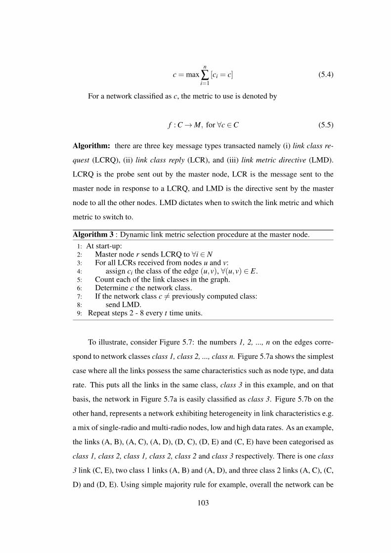
c = maxn

∑i=1

[ci = c] (5.4)

For a network classified as c, the metric to use is denoted by

f : C→M, for ∀c ∈C (5.5)

Algorithm: there are three key message types transacted namely (i) link class re-

quest (LCRQ), (ii) link class reply (LCR), and (iii) link metric directive (LMD).

LCRQ is the probe sent out by the master node, LCR is the message sent to the

master node in response to a LCRQ, and LMD is the directive sent by the master

node to all the other nodes. LMD dictates when to switch the link metric and which

metric to switch to.

Algorithm 3 : Dynamic link metric selection procedure at the master node.1: At start-up:2: Master node r sends LCRQ to ∀i ∈ N3: For all LCRs received from nodes u and v:4: assign ci the class of the edge (u,v), ∀(u,v) ∈ E.5: Count each of the link classes in the graph.6: Determine c the network class.7: If the network class c 6= previously computed class:8: send LMD.9: Repeat steps 2 - 8 every t time units.

To illustrate, consider Figure 5.7: the numbers 1, 2, ..., n on the edges corre-

spond to network classes class 1, class 2, ..., class n. Figure 5.7a shows the simplest

case where all the links possess the same characteristics such as node type, and data

rate. This puts all the links in the same class, class 3 in this example, and on that

basis, the network in Figure 5.7a is easily classified as class 3. Figure 5.7b on the

other hand, represents a network exhibiting heterogeneity in link characteristics e.g.

a mix of single-radio and multi-radio nodes, low and high data rates. As an example,

the links (A, B), (A, C), (A, D), (D, C), (D, E) and (C, E) have been categorised as

class 1, class 2, class 1, class 2, class 2 and class 3 respectively. There is one class

3 link (C, E), two class 1 links (A, B) and (A, D), and three class 2 links (A, C), (C,

D) and (D, E). Using simple majority rule for example, overall the network can be

103

A B

C

D

E

3

3

3

3

3

3

(a) Scenario A: homogeneous links

A B

C

D

E

1

2

2

2

3

1

(b) Scenario B: heterogeneous links

Figure 5.7: Conceptual depiction of network classification based on node and link charac-teristics.

classified as class 2. Alternatively, a weighted sum approach can be integrated in

the decision making process.

5.4 Performance evaluationTo demonstrate how the augmentation approach works with a given base-metric,

this study considers hopcount and ETX, which are common link metrics used in

WMNs routing. In addition, Airtime, which is the default routing metric used in Hy-

brid Wireless Mesh Protocol (HWMP) is also included. Besides their widespread

adoption, attention is drawn to these three metrics because they have the same ag-

gregation operator, which is addition (+). Additionally, they also use the same

order relation i.e. in all three cases, the metric value i is better than j iff i < j.

To test the dynamic link selection concept, a modified version of HWMP was

developed that included a component that assesses the network and sets the link

metric based on network characteristics as described in section 5.3.5. The network

assessment process runs at start-up and thereafter periodically. The modified pro-

tocol version is hereafter referred to as m HWMP. The presupposition made in this

study is that changes in network conditions necessitating a switch in the set link met-

ric will occur at long intervals and as such, it is expected that the gains of switching

104

metrics will outweigh the cost.

5.4.1 PHY layer modelling

The PHY model comprise channel loss and delay model based on the model detailed

in YANS [139].

5.4.2 Routing protocol description

For evaluation purposes, HWMP [137], which is the default protocol for IEEE

802.11s WMN was used. HWMP supports on-demand and proactive modes of

operation depending on the configuration.

5.4.3 Simulation scenarios and setup description

Evaluation was conducted in a simulation environment using Network Simulator

version 3 (NS-3) [140]. NS-3 is a Discrete-event simulator (DES) that can be con-

figured to produce deterministic results or stochastic output based on an inbuilt

pseudo random number generator. The default fixed deterministic seed value was

used throughout the simulations, while run numbers 1, 2, ..., 23 were used to get a

broader sense of results . The output of a deterministic model is determined by the

set of parameter values, which implies that the output of each run is the same unless

there is a change in parameter values. This is on the contrary to stochastic models

that are characterised by elements of chance and probability. As such, the output

of a stochastic model may vary given the same parameter values. The determinis-

tic approach was chosen in this study because it fosters reproducibility of results,

which helps with further research. The style of reporting used in this section and

subsequently other parts of this dissertation makes use of Strengthening The Report-

ing of Empirical Simulation Studies (STRESS) guidelines [141] and the references

therein. STRESS guidelines are aimed at providing a standardised approach for

reporting on discrete-event simulation-based operational research. The guidelines

emphasise providing adequate detail of the modelling as well as software/hardware

specifics to foster reproducibility of studies.

Figures 5.8a - 5.8c show the general layout of nodes used to compare perfor-

mance of base link metrics with the augmented variant. The setup shows clearly

105

1 11

destination

source

2

4 5

6 7

3

9 108

ETX pathAugmented ETX path

(a) ETX vs augmented ETX.

1 11

destination

source

2

4 5

6 7

3

9 108

subject to spectral noise

Airtime pathAugmented Airtime path

(b) Airtime vs augmented Airtime.

1 11

destination

source

Mesh nodeRoot mesh pointHop-count pathAugmented hop-count pathPossible routeRoot mesh point with low datarate

2

4 5

6 7

3

9 108

(c) Hop-count vs augmented hop-count.

Figure 5.8: Overview of network scenarios used to compare base metric with augmentedmetric.

marked sender and receiver node pairs and the path selected by the routing protocol

using the base metric and its augmented variant. The topologies are intentionally

simple to facilitate rigorous analysis. The network was simulated initially with uni-

form data-rate to trace the packets and establish the path chosen by the protocol

based on the metric as illustrated in the Figure. In latter simulations the sensitivity

of the metric to changes along the path was studied by varying the data-rate and

introducing spectral noise at the root mesh point along the protocol’s preferred path

as indicated in Figure 5.8b. To achieve multiple data-rates, the DataMode node

attribute setting in ns-3 was varied to mimic low and high data-rates. Using aug-

mented hop-count and augmented ETX metric, links with higher data-rate got a

higher priority while nodes with lower data-rate got a lower priority as discussed in

the next section. This concept can easily be extended to support several data-rates

by defining intermediate levels of priority between the lowest and highest priority.

106

Table 5.4: Simulation configuration

Parameter Setting

Node spacing 100 mNode mobility staticPHY specification 802.11Antenna Omni-directionalRouting protocol HWMP (proactive mode)Transport protocol UDPPacket size 1024 bytesNumber of flows variableSimulation time 100 sSeed value 1Run numbers 1, 2, ..., 23Simulator version ns-3.25

Table 5.4 shows a summary of the simulation settings used. The complete source

code and further simulation environment specific settings is accessible online [142].

5.5 Discussion of findingsFigures 5.9a, 5.9b and 5.9c show the performance in terms of throughput, mean

delay and jitter respectively, yielded by the routing protocol using the metrics under

consideration. The augmented metric variant exhibited performance improvement

in terms of throughput and delay. Hop-count on the other hand, outperformed all

the other metrics in terms of jitter.

When hop-count metric was tested in the network scenario depicted in Figure

5.8c, the protocol yielded lower throughput. This is because the protocol chooses

the path with least hop-count, whereas the augmented version of hop-count priori-

tises the path with a higher data-rate thereby producing higher throughput. Simi-

larly, when ETX was tested in the network layout shown in Figure 5.8a, the protocol

selected the path with minimal path ETX. Whereas using the augmented ETX vari-

ant, the protocol was able to consider path ETX and additionally favour links with

a higher data-rate. As a result, the augmented metric variant exhibited performance

improvement in terms of throughput and delay. Equivalently, the basic Airtime

metric failed to appropriately rank the optimal path under the set-up depicted in

107

Figure 5.8b because of its agnosticity to spectral noise. By augmenting Airtime

metric to factor in noise, the routing protocol was able to select the path comprising

links with higher data-rates and low noise. Subsequently, a Airtime returned better

performance compared to Airtime metric.

Proactive mesh protocols send hello packets at intervals in the order of sec-

onds, which is useful in quickly establishing alternative routes when a preferred

link goes down. One obvious drawback to the augmented approach is that it in-

evitably increases the size of hello packets to include the additional information.

However, DSA-induced link factors do not change significantly every couple sec-

onds. Therefore, at the routing protocol level, we can rip the benefits of carrying

out accurate link ranking by active probing or mathematical predictive analysis at

longer time intervals to lessen the overall impact of probing or computational costs.

This research proposes an n-tiered approach in setting the update interval i.e. using

different intervals for different factors. For example, channel information changes

less frequently and so, the hello packet only needs to include channel information

at intervals in the order of hours or days. Alternatively, these control messages can

be scheduled to occur at fixed off-peak times to minimise the impact of overhead

traffic.

0

2000

4000

6000

hopco

unt

a_hopco

unt

etx

a_etx

airtim

ea_airtim

e

Link metric

Ave

rag

e t

hro

ug

hp

ut

(kb

ps)

(a) Average throughput

0e+00

2e−04

4e−04

6e−04

hopco

unt

a_hopco

unt

etx

a_etx

airtim

ea_airtim

e

Link metric

Me

an

de

lay (

s)

(b) Mean delay

0.00

0.02

0.04

0.06

hopco

unt

a_hopco

unt

etx

a_etx

airtim

ea_airtim

e

Link metric

Me

an

jitte

r (s

)

(c) Mean jitter

Figure 5.9: Performance results.

108

Furthermore, the metric calculation process makes use of a measurement win-

dow i.e. a period over which probes are received. Reducing the window size results

in routing decisions that are more responsive to rapid fluctuations in link quality.

The advantage of high responsiveness is that at a given instance, the protocol is able

to find high throughput paths. However, the heightened sensitivity to changes in link

quality also causes more route flapping. Excessive route flapping can significantly

increase packet loss. Therefore, this study recommends a moving measurement

window similar to TCP’s sliding window.

Besides choosing the best forwarder based on the metric value received or

calculated, the routing protocol design has to put into account the trade-off be-

tween global and local optima. For instance, data-rate, which is a possible reward

parameter to factor into a metric is inversely related to transmission range. Con-

versely, Modulation and Coding Schemes (MCS) typically employ rate adaptation

techniques based for example, on signal strength to maintain optimal “goodput”.

The transmission speed listed by the driver indicates the wireless device’s modula-

tion rate, which may not necessarily be equal to the usable throughput. However, it

provides a good indication of the device’s throughput capability. All in all, further

investigation is needed to thoroughly understand the interrelation among reward and

penalty parameters, global and local optima.

5.5.1 Scalability

One of the major concerns regarding A-link-metric is scalability. To address such

concerns, analysis of scalability defined in terms of network convergence was car-

ried out. The method and findings are presented in Appendix B. The results show

no significant difference in scalability between the augmented metric solution and

the corresponding base metric. This confirms the expectation that scalability has

little to do with the metric component and more to do with the routing protocol as a

whole.

109

5.5.2 Implication of the findings

i Explicit factoring. Thorough experimentation may be required in some in-

stances to establish whether or not a piece of information is redundant. For

example, in most MCS implementations, the data-rate is regulated based on

the signal to noise ratio (SNR). Hence at first glance, combining data-rate and

SNR into the metric might appear redundant because the two may be seen

as capturing the same link characteristic. However, simulation results show

an observable performance boost when SNR and data-rate are explicitly fac-

tored into the metric. Furthermore, while variables may be highly correlated

in principle, they may not in practice correlate as highly due to a range of

issues such as driver and hardware limitations. Therefore, explicitly factoring

the variable(s) into the metric is essential for effective routing.

ii No all-round ideal metric. Metrics perform differently under different sce-

narios. As new routing protocols are developed to harness DSA dividends,

support for multiple metrics and easy integration of new ones should be a

core design objective.

iii Dynamic metric selection. Once there is support for multiple metrics as well

as metric calculation algorithms, the next step is to in-build the routing proto-

col with the “intelligence” to dynamically select the suitable metric based on

the prevailing network status.

5.5.3 Limitations of the study

i The enormous complexity associated with modelling a wireless channel sug-

gests that results obtained from a simulation environment only give an ap-

proximation of performance, but serve well as a guide nonetheless.

ii The characterisation of the network for purposes of determining suitable link

metric employed in dynamic link metric selection was to an extent influenced

by the test results obtained through this ns-3 simulation setup. The results

obtained from other simulation environments may be different due to lack of

consistency in simulator package implementations.

110

iii Network performance does not depend on the sufficiency of the link metric

alone, but also on the routing algorithm and protocol implementation. The re-

sults presented herein are specific to the routing protocol considered. Follow

on work will include an extension of the study to cover other protocols.

5.6 Chapter summary and future workThis study confirms that base metrics are inadequate and that augmented alterna-

tives would be better for DSA. This research makes no claim about a single suitable

routing metric, but instead provides a framework for taking a desired existing metric

and adapting it for DSA.

The study has demonstrated basic scenarios under which a routing protocol

might fail to compute the optimal path using the metrics considered. Suffice to say

that for every scenario under which a routing protocol with its associated metric

thrives, there is always another set-up or network state under which it performs

poorly. Based on this observation, it is evident that routing protocols should always

be designed to support multiple routing metrics and dynamically toggle the link/-

path valuation scheme for optimal performance in different deployment scenarios.

The discussion on routing is going to remain relevant for as long as there is demand

for higher QoS for various wireless network services. It is difficult to maximise

performance in all desired terms because several performance objectives such as

transmission rate and transmission range are antagonistic. Consequently, courses of

action taken to maximise one objective tends to minimise the other. More research

is required to resolve the ensuing conflict graph.

Although wireless network routing metrics have been studied for a long time,

there is yet to emerge a single agreed upon routing metric. This goes to show that

the choice of routing metric in a multi-path environment is not a settled matter yet.

There is still plenty of room for improvement, and thus further inquiry should con-

tinue to challenge the current ideal. As we prepare for the adoption of the dynamic

link metric selection concept in emerging and existing routing protocols, future

work will include the following further investigations:

111

i Criteria/techniques for network assessment and classification. Suppose met-

ric A is suitable for a network with static nodes and metric B is ideal for a

network with mobile nodes. Now posit the network consists of some nodes

that are static and nodes that are mobile, there is a question of which metric

the routing protocol should use between A or B. The current DPMeS strategy

uses simple majority rule to classify the network, which means that if there

are more static nodes than the ones that are mobile, then the network will be

classified as static. This may lead to a suboptimal solution, therefore further

research is required in that direction.

ii The frequency with which to assess the network and fine-tune the assessment

process for practical purposes. There is ample evidence to support the pro-

posed assessment criteria, however the points of transition for determining

factor(s) i.e. exact points where performance using one metric begins to de-

teriorate and the performance of the other metric starts to get better are still

only vaguely clear. For example, the question of “what extent and degree of

mobility is required for hop-count to outperform ETX?” still needs further

investigation.

iii The inter-play among the link metric, routing protocol and the choice of val-

ues for the tuning parameters α and β . The relationship among the afore-

mentioned aspects is not adequately understood at the moment. One possible

line of enquiry worth exploring is to investigates trends (if any) in the validity

of these scaling constants and explore the option of dynamically sizing the

values.

iv Test-bed implementation to confirm the simulation results. There is a lack

of standardisation across network simulation packages. In addition, several

wireless network aspects such as channel quality and interference are hard

to model realistically. Therefore, a test-bed implementation is imminent to

promote further adoption and refinement of this work.

112

Chapter 6

Characterisation of 5 GHz WiFi and

UHF-TVWS hybrid links

Network capacity and performance can be improved by using multiple channels

simultaneously, which requires multiple transceivers. Basic multi-channel capable

nodes can be built using one of the following architectures: (i) multiple hardware

platform where two or more single-radio nodes are connected via Ethernet to form

one logical multi-radio mesh router; (ii) single hardware platform where a single

node has multiple transceivers fitted; or (iii) single-chip multi-transceivers where

multiple transceivers are integrated into one wireless chipset on a router [88]. This

study considers the single hardware platform fitted with multiple transceivers ap-

proach. The focus is on mesh routers fitted with 5 GHz WiFi and UHF-TVWS

transceivers to realise multi-band-multi-radio mesh routers. Spectrum availabil-

ity varies from location to location, but is generally inversely proportional to the

population density. WiFi is suitable for densely populated urban areas, whereas

UHF-TVWS is ideal for sparsely populated rural areas, which also happen to have

significantly more TVWS compared to urban communities.

When confronted with diverse population densities, there exists a grey region

(sometimes referred to as peri-urban) that is characteristically a cross between rural

and urban regions from a spectrum requirement standpoint as shown in Figure 6.1.

A combination of WiFi and TVWS is appropriate in this region of intersection.

Research [143] has shown that in such scenarios, the gains of using a combination of

113

Urban Rural

Characteristics:abundant spectrum sparse populationpoor connectivity

Ideal spectrum:lower frequency

long range e.g. UHF TVWS

Characteristics:spectrum crunch dense population

Ideal spectrum:high frequency

short transmission range e.g. WiFi

Peri-urban

Figure 6.1: Spectrum requirements by region.

TVWS and WiFi are much larger compared to WiFi-only or TVWS-only spectrum

band usage.

Applications of WiFi and TVWS can be categorised coarsely into access-tier

and back-haul-tier network architectural components. For a combination of techni-

cal and economic reasons, several reports from literature have shown deployment

scenarios where any single operating band is inadequate, which points to the fact

that an optimal solution requires a mixture of operating bands at the access as well as

the back-haul tier. Notable examples of proposals made by the research community

include, a combination of WiFi and LTE [144], and a combination of TVWS and

LTE-A [145]. The problem of optimal use of TVWS and WiFi bands for back-haul

connectivity amid diverse population densities is highlighted in WhiteMesh [143].

WhiteMesh introduces a Band-based Path Selection algorithm designed for optimal

channel assignment of both TVWS and WiFi. The WhiteMesh solution is analysed

in terms of traffic served putting the population density into account, but does not

consider environmental factors that affect link performance. Other researchers have

proposed combining TVWS with 5G infrastructure for rural coverage where tradi-

tional cellular coverage models are less economically viable due to low user density

114

and subsequent revenue [146]. The work on TVWS with 5G considers the cost and

analyses the feasibility of using TVWS for rural Internet access using 5G, but does

not provide any test results of TVWS performance for the proposed architecture.

Overall, there is limited experimental studies comparing the performance of links

operating in 5 GHz and UHF-TVWS radio frequency bands.

Regarding the performance of WiFi-like access points operating in TVWS, the

benefits of larger coverage area and better obstacle penetration are challenged when

inter-access point interference is considered [147]. The lower operating frequency

of TVWS results in larger cell sizes and the overlap in contention domains among

interfering access points significantly reduces the link rate. Therefore, it may be

said that the wider coverage range provided by TVWS is considered best suited to

rural settings because degradation due to inter-access point interference is minimal

because of low access point density as a result of sparsity in population. However, a

few judiciously well placed TVWS radios spaced far apart in urban areas can offer

lower data rate coverage filling and better building penetration, which is useful in

bridging the gaps among clusters of high frequency WiFi radios as illustrated in

Figure 6.2.

High frequency APLow frequency AP

Figure 6.2: Densely spaced high-frequency (e.g 2.4/5 GHz) access points combined withjudiciously placed low-frequency (e.g. UHF-TVWS) access points at the ac-cess layer in urban communities.

115

6.1 Envisaged application scenarioOne of the biggest challenges facing rural communities is the extension of con-

nectivity from the nearest point-of-presence (POP) to the houses. These areas are

typically characterised by sparse population and rugged terrain, which makes it

economically and technically impractical to lay down copper or optical fibre cables.

Moreover, vegetation and other obstacles along the signal propagation path results

in obstructed line-of-sight.

Owing to the known advantages and drawbacks of high and low operating radio

frequencies, this work considers using a combination of WiFi operating in 5 GHz

and TVWS for first-mile connectivity. The term “first-mile” is hereby defined as

the stretch from the location of the remotest user to the closest POP. Figure 6.3

illustrates the envisioned application scenario. The architecture comprises nodes

with 2.4 GHz WiFi, 5 GHz WiFi and UHF-TVWS radios strategically deployed at

key community sites such as schools, clinics, libraries, office parks and houses. The

2.4 GHz radio serves the access-tier whereas the 5 GHz WiFi/UHF-TVWS radios

interconnect the nodes in mesh mode to form the back-haul-tier.

Figure 6.3: Envisaged application scenario using a combination of high frequency radiosand low frequency radios such as 5 GHz WiFi and UHF-TVWS to extendbroadband connectivity.

116

6.2 Problem description and formalisationGiven the required combination of radios described in the previous passage, this

section describes the problem of link selection and the opportunities for multi-band-

multi-radio enabled WMN routers. Granted node pairs with WiFi and UHF-TVWS

radios, there are nine possible link configurations as the Alice & Bob topology in

Figure 6.4 illustrates.

(a) select 5 GHz WiFi (b) select TVWS (c) use 5 GHz WiFi totransmit and TVWS toreceive

(d) use TVWS to transmitand 5 GHz WiFi to re-ceive

(e) aggregate 5 GHz WiFiand TVWS into a sin-gle logical link to trans-mit/receive

(f) use 5 GHz WiFi totransmit only andTVWS to transmit andreceive

(g) use 5 GHz WiFi to re-ceive only and TVWSto transmit and receive

(h) use 5 GHz WiFi totransmit and receive,TVWS to transmit only

(i) use 5 GHz WiFi to trans-mit and receive, TVWSto receive only

Figure 6.4: Possible link options when using hybrid links. The black solid line and bluedashed line respectively represent 5GHz WiFi and UHF-TVW radios.

To generalise, we first consider two wireless devices, node A and node B. Each

of these devices has a number of wireless interfaces, which can form connections

between the two devices in a variety of configurations and permutations. A wireless

117

interface is one wireless radio card using a specific technology, spectrum band and

channel (e.g. 2.4 GHz WiFi, 600 MHz TVWS, LTE etc.) and antenna on board

the device (say A) that can transmit or receive on one logical path to another like

interface on another radio device (say device B). Successful transmission is only

possible between two interfaces that are alike in centre frequency, bandwidth, and

MAC technology. We model this situation as a bipartite graph G = (A,B,E), where

A and B are interfaces on the radio device. There are several ways that devices A

and B can form connections. Consider the different options of technology and band

that can be used, and possible combinations of these links with parallel links and

link aggregation as shown in Figure 6.4. Each individual interface-to-interface link

is modelled as a directed edge E in the graph model. An edge can be in one of a

number of states, for example we may define the possible states as incident or trans-

mitted. The set of possible edges on one device must be combined with the set of

possible edge states on the second device. It is clear that as the number of interfaces

on a device increases the number of possible link configurations grows rapidly. If

we assume the wireless devices have a uniform number of radio interfaces, the total

number of possible link configurations n is given by

n = (pr−1)k for p,r,k ∈ N (6.1)

where p is the number of possible edge states, k is the number of nodes and

r is the number of wireless interfaces. The “−1” term is to remove the empty set,

which is not a valid link configuration.

The system aims to find the set of link configurations:

S = S j := y ji 7→mini

z ji(x)

where j = 1,2, ...,N−1 and i = 1,2...,n for j 6= i(6.2)

where x = amount of data to be served, y = link, z = transmission time, which

depends on interference, congestion, etc. and is handled by the MAC protocol, and

n = number of possible links, which is dependant on the number of radios per node.

118

6.2.1 Single point-to-point

Suppose there are two nodes A and B, which is the simplest case scenario, the so-

lution to the link selection problem at any given moment is going to be one of the

options presented in Figure 6.4. It is very easy to determine the optimal link in

one of extreme deployment scenarios where only one radio is operational for one

reason or the other. For example, in an area where there is no TVWS available, 5

GHz WiFi becomes the only option. Another example is when the node spacing is

beyond WiFi’s transmission distance, in which case TVWS becomes the viable op-

tion because UHF-TVWS attenuates less compared to WiFi as explained by Friis’

path-loss model [148]:

L f s = 20log10( f )+20log10(d)+32.45 (6.3)

where L f s is the path loss in dBm relative to mW, f is the operating frequency

in MHz and d is the distance in km. The focus of this dissertation is on a typical

scenario where both WiFi and TVWS are operable with performance subject to

prevailing spatial/temporal spectral and environmental conditions.

For a one-hop scenario i.e. two wireless radio devices communicating only

with each other (local optima), the link selection scheme chooses a link configu-

ration yi from the set of possible link configurations of size n to transmit a data

package of size x in the minimum possible time. The time taken for that package

transmission on that specific link configuration is zi(x).

yi 7→mini

zi(x) : i ∈ 1,2, ...,n

In the case of multi-hop system (global optima) of N identical radio de-

vices, the link selection method chooses a link configuration for each hop S j,

j ∈ 1,2, ...,N−1 such that the total transmission time is minimised. Disregarding

buffer size constraints and the potential impact of multi-path interference, the total

119

link selection set can be denoted as

S = S1,S2, ...,SN−1

S j ∈ S := y ji 7→mini

z ji(x) : j, i ∈ N

The results discussed in section 6.5 show that performance of these links de-

pends highly on the combination of parameter settings such as channel, transmis-

sion power (txpower), channel width, modulation and coding scheme (MCS), and

environmental factors.

6.2.2 Point-to-multi-point

Suppose there are three nodes A, B and C connected as shown in Figure 6.5. When

node A has a queue of data destined for node B and another queue for node C, it can

aggregate the links, send to node B in one timeslot and send to node C in another

timeslot. Alternatively, node A can send to node B on one interface and send to

node C on the other interface. For point-to-multi-point, we aim to choose the set of

links S j, where in this case, j = 1,2, ...,N−1 for N-1 nodes connected to a single

node.

S j := y j 7→mini

z ji + τ (6.4)

where τ = delay associated with media contention.

There are two requirements: (i) a routing protocol capable of exploiting avail-

able link options and (ii) a suitable routing metric to aid the protocol in determining

the optimal option.

A

B

C

Figure 6.5: Transmission options for a basic point-to-multi-point link.

120

6.2.3 Multi-point-to-multi-point

The term multi-point-to-multi-point is used in this context to describe a generalised

scenario arising from mesh network formation in which nodes connect in ad-hoc

fashion. The routing task of selecting an optimal link in this scenario is to a signifi-

cant extent partly a scheduling problem and therefore the solution may be described

as “best effort”.

6.3 Hybrid-link utilisation modelFigure 6.6 shows the proposed three-tired multi-link utilisation framework along

with an implementation example. This section discusses the three layers and sub-

components, and highlights optimisation approaches at each layer.

6.3.1 Virtual interface

Virtual interface is the logical connection point to the wireless mesh network. This

is the interface that is “visible” to the higher layers of the network protocol stack.

By virtualising the interface used by the mesh routing protocol, multiple virtual

interfaces can be created thereby allowing a single node with possibly a single radio

to join and participate in multiple mesh networks if desired.

6.3.2 Link permutation

Link permutation defines the possible link options described in section 6.2, which

depends on the number and type of radios. The routing protocol elects the link

option from among possible permutations in a way that is similar to how the next-

best-hop is selected. Link performance is influenced by factors internal and external

to the network. As such, quality assessment of individual radio links is required to

rank the link options. Owing to the unpredictable nature of wireless links, this

dissertation proposes dynamic selection of the optimal link option from among the

possible permutations. The immediate challenge is to develop routing algorithms

capable of determining not just the locally optimal link option, but a link option that

is optimal end-to-end.

In section 6.2, equation 6.1 was derived that expresses the number of possible

121

Virtual interface(s)

Physical interface(s)

Link permutation

Virtual la yerMulti-link policy

Algorithm

(a) Proposed framework

Mesh interface

Split Aggregate

WiFi TVWS

Select

(b) Implementation example involving WiFi andTVWS hybrid links.

Figure 6.6: Multi-link utilisation framework.

link permutations in terms of k the number of nodes and r the number of radios on

each node. As the values of k and r increase, the number of possible link options and

information about the options increases aggressively as shown in Figure 6.7. For

examples, as little as ten nodes yield 59049, 282475249, and 576650390625 possi-

ble link options for two, three and four radios respectively. This could be beneficial

on one hand, for example if resilience and fault tolerance are the ultimate goals.

122

0

30

60

90

120

0 25 50 75 100

Number of nodes

Lo

g10 (

nu

mb

er

of lin

k o

ptio

ns

) Number of radios

2

3

4

Figure 6.7: Link permutation analysis.

But on the other hand, findings from other fields of research such as marketing re-

search regarding short-listing of candidate options show that it gets increasingly

difficult to find the right candidate as the number of options and the information

about the options increase [149]. The larger evaluation costs associated with the in-

crease in choices and criteria results in a smaller consideration set [150]. Applying

this reasoning from a human perspective to the mesh routing context lends way to a

prediction that an increase in the number of link options may not necessarily trans-

late into improved performance. As a matter of fact, the ensuing complexity could

make it infeasible to pre-compute the quality of each and every option. For that

reason, this dissertation identifies and focusses on three main link options, namely

single-I/O, split and aggregate. The term single-I/O is being used to refer to a link

consisting of a single-radio transceiver. On the other hand, a split link refers to a

configuration where a node dedicates one radio to sending packets and the other for

receiving. An aggregate link is when two or more radios are combined to form a

single logical link for purposes of increasing throughput. These three are the key

hybrid-link configuration approaches. The rest of the options identified in section

6.2 can be considered as shadows of these three principal options.

123

In related works, the split link concept is typically applied as a way of load-

balancing. This dissertation extends this view and presents link splitting as a link

asymmetry mitigation technique. A splitting opportunity exists when the high and

low throughput of individual radios is in opposite directions as illustrated in Figures

6.8a and 6.8b. The splitting opportunity may result from RF interference, hardware

Radio 1

Higher throughput

A BLower throughput

(a) Radio 1 only.

Radio 2

Lower throughputA B

Higher throughput

(b) Radio 2 only.

Radio 1 and radio 2

High throughput

A BHigh throughput

(c) Radio 1 and radio 2

Figure 6.8: Radio link splitting opportunity.

imperfections and other causes. To illustrate, consider Figure 6.9: node B strategi-

cally placed at a high site and close to heavy duty television broadcast transmitter

towers experiences a significant amount of RF noise in the UHF band. On the other

hand, node A, located at a lower site somewhere in a residential area farther away

from TV transmitters experiences a nominal amount of interference in the UHF

band, but the 5 GHz WiFi radio gets affected by other WiFi devices nearby. The

term ‘close’ is being used in this context to refer to the combined effect of geo-

graphical as well as spectral proximity to the source of interference 1.1When a TVWS device operates on channel x and there are other strong TV transmitters using

channel x+ 1 within interference range, the TVWS device is said to be spectrally close to the TVtransmitter. Previous investigation[151] has shown the adverse effect that close spectral proximityof TV transmitters has on the throughput of TVWS nodes.

124

5 GHz WiFiUHF-TVWS

Node B:at a high site, close

to TV transmitters, more noise in the

UHF tv band

Figure 6.9: Link asymmetry caused by primary transmitters and other sources of strong RFsignals interfering with wireless mesh routers. Faulty circuitry or misconfigu-ration can also result in link imbalances.

Under these conditions, when node A sends data to node B using the UHF link,

there is a significant amount of packet loss at reception. Similarly, when node B

sends data to node A via the 5 GHz interface, high packet loss is expected. Thus

the splitting opportunity could be a permanent state of a link or an intermittent

occurrence, hence the need for a dynamic selection mechanism. Regardless of the

underlying cause, the key consideration when splitting radios comes down to the

choice of uplink and downlink interfaces as illustrated in Figure 6.8. For example,

with respect to node A in Figure 6.8, by splitting the link such that each node has

the “best foot put forward” i.e. radio 1 serves the uplink while radio 2 serves the

downlink, higher throughput can be achieved in both directions of communication

between node A and node B as reflected in Figure 6.8c.

125

6.3.3 Multi-link policy and algorithms

The multi-link policy sets out the over-arching performance objective, which might

be achieving fault tolerance, maximising throughput, load balancing and so forth. A

network may adopt one or more policies depending on performance requirements.

Algorithms in turn specify the policy implementation detail. Some example poli-

cies and algorithms that can be applied on an aggregated link are hereby discussed

below.

1. Round-robin. Packets are transmitted across all the aggregated interfaces se-

quentially starting from the first available interface to the last. This approach

provides fault tolerance and load balancing. The drawback of round-robin

in its basic form is that if the radios have different transmission rates, the

low data-rate interface creates a bottleneck. Thus effective throughput gets

determined by the radio link with the least capacity.

2. Broadcast. Each packet to be sent is duplicated and transmitted on all avail-

able interfaces for redundancy. Typically, this policy is not applied as a direct

throughput enhancement approach. Instead, it is aimed at achieving fault tol-

erance as sending out multiple copies of packets maximises the chances of

delivery.

3. Active-backup. This is a multi-link usage policy where one radio is des-

ignated as the “primary” transceiver. The second available radio gets acti-

vated only when the active radio fails. This could be applicable in scenarios

where there are costs associated with using a particular alternative radio. In

such cases, instead of using multiple radios in parallel to increase capacity, it

makes sense to use the costly fallback link on a as-needed-basis.

4. Network coding. The basic principle of network coding is to combine multi-

ple packets into a single transmission as opposed to having multiple transmis-

sions. This approach aims to improve performance by reducing the number of

transmissions thereby minimising contention/media access delays. Since the

introduction of the idea [152], several network coding and decoding schemes

126

have been developed [153], [154], [155], [156]. Just as is the case with aggre-

gation and splitting, an opportunity for network coding has to first be identi-

fied. A network coding opportunity exists if node A and node B are both able

to overhear the relay node. Once the opportunity is identified, the relay node

buffers packets meant for node A and node B, but instead of transmitting to

node A and then to node B, the relay node codes the packets and sends at

once. Node A and node B in turn decode the packet and they each get the

packet addressed to them.

While multi-link policies are chosen based on the desired performance objective,

the achievable performance gains remain dependent on availability of the oppor-

tunity such as a network coding opportunity described above or the radio splitting

opportunity described in section 6.3.2. This dissertation recommends optimisation

with loose coupling design approach to ease the interchange and combination of

policies and algorithms with the different link permutations e.g. combining link

aggregation with network coding.

6.3.4 Physical interface

Physical interface refers to the underlying physical wireless network cards. There

is substantial motivation for using multiple radios. This includes the need for both

high and low operating frequencies to meet technical or regulatory requirements

as explained in the chapter introduction or simply as a way to increase network

capacity.

6.4 Experimental evaluationThe objective of the study was to investigate the performance of the different 5 GHz

WiFi and UHF-TVWS radio settings, namely channel, channel-width, and transmis-

sion power (txpower) under different environmental conditions such as trees/vegeta-

tion, building structures and landscape that tend to affect line-of-sight. The physical

setup comprised a specially designed multi-radio mesh router with 5 GHz and UHF-

TVWS antennas, and a portable power source for powering the device as shown in

Figure 6.10. Table 6.1 lists the specifications of the equipment used in the exper-

127

iment. The experimental performance measurement exercise started off with an

indoor setup to benchmark performance and calibrate the equipment prior to setting

up the experiment outdoors. The indoor setup comprised nodes set up inside the

research lab2 such that node A and node B were 21 m apart, and 1 m, 0.9 m and

4.5 m away from the wall sides while the TVWS antenna stood at 0.36 m below

the ceiling as shown in Figure 6.11. This was followed by outdoor experiments

setup to measured performance of 5 GHz WiFi and UHF-TVWS in three scenarios,

namely clear line of sight, near line of sight obstructed by trees, and near line of

sight obstructed by building structures as shown in Figures 6.15 and 6.17. Figure

6.13 shows the aerial view of the measurement site.

1.84 m

2.34 m

Power supply

TVWS antenna

5 GHz antenna

Mesh node

Figure 6.10: Outdoor setup

2Centre in Information and Communication Technologies for Development (ICT4D) lab, Com-puter Science building at the University of Cape Town.

128

The measurement process involved mounting the setup on two ends of a site

to capture the environmental variable of concern. Performance was measured using

iperf and ping tools for different combinations of channel, txpower and channel

width settings. The process was controlled from a laptop (not visible in the picture)

connected to the node over a dedicated 2.4 GHz WiFi access connection. A custom

measurement script was developed for this purpose that executed control commands

between node pairs over a dedicated control link established using 3G modems.

Techniques such as ssh port forwarding were used to circumvent the 3G service

provider’s Network Address Translation (NAT) server or firewall by establishing

a reverse ssh tunnel. In addition to facilitating remote control of the setup, the

dedicated control link ensured that the data collection process had minimal impact

on the experiments conducted on the 5 GHz WiFi and UHF-TVWS links.

Table 6.1: Node specifications.

WiFi TVWS

i) System board: MikrotikRB433

ii) Operating system: OpenWRT

iii) WNIC: Atheros-based 802.11a/b/g mini PCI adapters.

iv) Antenna:

• Brand: made/dis-tributed by scoop(www.scoop.co.za)

• Model: ANT-P523

• Gain: 23 dBi

• Frequency: 5150 - 5850MHz

• Cable type and length:coax, 1 m

i) System board: Mikrotik RB433

ii) Operating system: OpenWRT

iii) WNIC: Doodle labs DL509-78Broadband Radio Transceiver forthe 470-784 MHz TV band.

iv) Antenna:

• Brand/Model: Maxview,MXR0053 TV Aerial -10element

• Forward Gain: 8 dB

• Front to back ratio: 10-20 dB

• Acceptance angle: 25

• Frequency range: 470-860MHz; channel 21-69

• Cable type and length: coax,1.55 m

129

(a) Node setup.

A B21 m 0.9 m0.9 m

1 m1 m

4.5 m

(b) Node spacing.

Figure 6.11: Indoor setup.

6.5 Results and discussion

6.5.1 Indoor performance

Figure 6.12 shows the relationship between throughput and transmit power observed

from the indoor setup. For the 5 GHz WiFi radio, throughput slightly increases

with transmit power. A more marked increase in throughput would be expect in

an outdoor real-world setup owing to the anticipated increase in SNR. The sus-

picion is that the reduced distance between the nodes reduces the possible range

of throughput values. Very surprisingly and counter-intuitively, once the transmit

power surpasses 10 dBm for TVWS, the throughput in fact decreases rapidly, which

completely contradicts Shannon’s Law. This is because of the input signal level at

the receiver being well above its recommended range, thereby causing saturation

of the electronics and distortion of the signal. The DL509-78 transceiver is quoted

to have a recommended input signal strength range of -40 to -80 dBm, while on

the TVWS interface the input signal levels were measured to reach above -30 dBm,

even climbing to +9 dBm in one measurement and above -20 dBm for a transmit

130

power of 20 dBm in several measurements. Such high input power values cause

the signal responses of the RF receiver front-end electronics to become distorted.

The operational amplifiers cannot output a voltage above their supply voltage in

response to a higher input power - i.e. they saturate at such high input signal levels

- so they are unable to reflect the variations in the received signal accurately, caus-

ing signal distortion and inability of the system to decode the signal correctly. On

the other hand, for the same transmit power values, the receiver-side 5 GHz WiFi

card showed lower input signal strength measurements, all falling below -40dBm,

so saturation and the resulting decreased throughput was not observed in the experi-

ments on the 5 GHz radio under the same conditions. This observation underscores

the point that considering signal strength alone can be misleading when assessing

link quality or determining optimal operating parameters as it clearly fails to reflect

possible link failure/deterioration due to phenomena such as power saturation. Fur-

thermore, it becomes important in these types of studies to isolate or distinguish

platform related characteristics from the properties attributed to the operating radio

frequency.

0

5

10

15

20

0 5 10 15 20

Tx power (dBm)

Thro

ughput (M

bits/s

ec)

Link

20 MHz, WiFi

20 MHz, TVWS

Figure 6.12: Throughput vs txpower at a short distance on a 20 MHz channel. A similartrend was observed for 10 MHz and 5 MHz channels.

131

6.5.2 Outdoor performance: clear line-of-sight

This round of experiments were conducted at the University of Cape Town (UCT)

rugby field shown in Figure 6.13, where clear-line-of-sight (marked by the solid

yellow line) was established. The distance between the two endpoints was approx-

imately 0.65 km. Figure 6.14 gives a synopsis of performance for radio links with

unobstructed line-of-sight. Overall performance in terms of throughput ranged from

zero to just under 15 Mbits/sec depending on the choice of operating channel, tx-

power and channel-width settings as shown in the figure. For example, the through-

put slot for 5 GHz WiFi channel 48, 20 dBm txpower and 20 MHz channel-width is

empty because there was no throughput for that combination of settings. The hori-

zontal line across the bar marks the throughput in the opposite direction while the

vertical lines indicate the standard error in the forward direction throughput mea-

surement. The results shown are only for 5 GHz WiFi and UHF-TVWS operating

on channel 48 and 11 respectively, however a similar pattern was observed on al-

ternative operating channels. The other observation is that at that distance, it can

generally be said that the 5 GHz WiFi link outperforms UHF-TVWS. Furthermore,

there was a marked difference in performance between busier and cleaner TVWS

channels. The results presented in this section were included in a paper [157].

Figure 6.13: Aerial view of outdoor measurement sites.

132

5 GHz WiFi UHF−TVWS

48.2

0.2

048.2

0.1

548.2

0.1

048.2

0.5

48.1

0.2

048.1

0.1

548.1

0.1

048.1

0.5

48.5

.20

48.5

.15

48.5

.10

48.5

.511.2

0.2

011.2

0.1

511.2

0.1

011.2

0.5

11.1

0.2

011.1

0.1

511.1

0.1

011.1

0.5

11.5

.20

11.5

.15

11.5

.10

11.5

.5

0

5

10

15

Channel, channel width and trxpower setting

Th

rou

gh

pu

t (M

bits/s

ec)

Figure 6.14: Performance of 5 GHz WiFi and UHF-TVWS links for different txpower andchannel width combinations. The bars are labelled x.y.z where x, y and zcorrespond to the operating channel, channel width (MHz) and txpower (dBm)respectively.

6.5.3 Outdoor performance: near line-of-sight

Obstructed by trees

The set of experiments to evaluate performance of a near-line-of-sight link ob-

structed by trees were done in the wooded area around UCT tennis courts shown

in Figure 6.13 on the previous page, marked by the dashed yellow line. The mea-

surement exercise proceeded as follows: one node was fixed on one end while the

second node was positioned such that a tree obstructed the line-of-sight as shown in

Figure 6.15, and throughput measured. The second node would then be repositioned

such that there was an incremental number of trees in between and performance

measured on each increment. The site had pine trees whose trunk circumference

measured approximately 2 m on average. The space between the trees from the first

to the last was as follows: 20 m, 28 m, 7 m, 9 m, 5 m, 18 m, 25 m. The spacing is

irregular because these are trees growing freely in nature.

Multiple data samples were collected for different combinations of settings.

The combination of channel, channel-width and txpower that gave the best results

at the highest tree count was then considered at all the other tree counts. For the

TWVS radio this turned out to be channel 7, 5 MHz channel-width, 5 dBm txpower,

133

whereas for the 5 GHz it was channel 44, 20 MHz channel-width and 20 dBm

txpower. The rationale behind this is that it is better to have a low-throughput link

that works end-to-end than a high-throughput link that breaks mid-way along the

path. Figure 6.16 shows the average forward and reverse throughput. From these

results, it is evident that a 5 GHz WiFi link breaks completely as soon as the link

is obstructed by more than two trees. On the other hand, a TVWS link is operable

with as many as eight trees obstructing the line-of-sight. Based on this observation,

the expectation is that the TVWS will still be operation if the extent of obstruction

and distance increase. The study was carried out in the middle of a wooded area, but

the analysis only considers the number of trees that would be covered if a straight

line was drawn between the two endpoints. Considering the effects of multi-path

fading, several other trees scattered about undoubtedly affected performance.

Figure 6.15: Setup of near line-of-sight link obstructed by tree.

134

0.0

2.5

5.0

7.5

10.0

1 2 3 4 5 6 7 8

Number of trees

Thro

ughput (M

bits/s

ec)

Link

5 GHz WiFi

UHF−TVWS

Figure 6.16: Throughput of UHF-TVWS and 5 GHz WiFi over a link obstructed by trees.

Obstructed by concrete building structures

Figure 6.17 shows one end of the setup mounted at UCT traffic Department area to

measure performance of a near-line-of-sight link obstructed by a concrete building

structure. Figure 6.18 shows the performance of the UHF-TVWS link for this setup.

Notice the absence of 5 GHz performance results for this setup. This is because the

5 GHz radio could not establish a link between the two endpoints. The throughput of

the 5 GHz radio remained zero for all possible combinations of operating parameter.

It was possible to adjust the degree of obstruction so to speak, by shifting the setup

ever so slightly either to the extreme left or extreme right of the building structure.

However, even with a reduced degree of concrete structure obstruction, the 5 GHz

link failed to work.

The experimental results confirm the theoretical expectation that high operat-

ing frequencies such as the 5 GHz band are suitable for short to medium distances

with clear line-of-sight. On the other hand, lower operating frequencies such as the

UHF-TVWS band perform better for long distance and obstructed line-of-sight. The

results also show that when a 5 GHz radio link is obstructed it breaks completely,

whereas a TVWS link still works albeit with degraded throughput depending on

the degree and extent of obstruction. There exists an interesting interplay among

the channel quality and channel width, and transmission power settings. Further

investigation is needed to gain more clarity on what constitutes optimal settings.

135

Figure 6.17: Link obstructed by a building structure. The other node (not visible) waspositioned behind the building structure and at a much lower position due tothe undulation of the ground.

Channel 1 Channel 4

1.2

0.1

51.2

0.1

01.2

0.5

1.1

0.1

51.1

0.1

01.1

0.5

1.5

.15

1.5

.10

1.5

.5

4.2

0.1

54.2

0.1

04.2

0.5

4.1

0.1

54.1

0.1

04.1

0.5

4.5

.15

4.5

.10

4.5

.5

0

2

4

6

8

Channel, channel width and trxpower setting

Thro

ughput (M

bits/s

ec)

Figure 6.18: Throughput of UHF-TVWS over a link obstructed by a building struc-ture. The blueish vertical lines indicate the standard error calculated as(standard deviation) ÷

√(sample size), while the orange horizontal lines

mark the link’s throughput in the reverse direction.

136

6.5.4 Vertical vs horizontal polarization

There were performance variations observed between vertical and horizontal polar-

ization, which may be attributed to differences in channel quality subject to polar-

ization. For example, a channel may be vertically occupied, but horizontally vacant

or vice-versa. Other than the channel quality, there is no statistical evidence to sug-

gest a difference in obstacle penetration/circumvention capability between vertical

and horizontally polarised radio antennas of either 5 GHz or UHF-TVWS radios.

6.5.5 Contextualizing performance results

To put the achieved throughput into perspective, consider Internet provisioning in

Macha, a rural village in Southern Zambia. The village was initially connected

to the Internet via a 256 kbps downlink and a 64 kbps uplink satellite connection

with a running cost of 1 200 USD per month. They later upgraded to a 2 Mbps

microwave terrestrial connection that costed 3 600 USD per month [9]. For rural

communities where the estimated average income is no more than $1 per person per

day, the setup costs plus these monthly recurring charges is grossly expensive. We

were able to achieve throughput above 2 Mbps using TVWS despite obstructions

across the link. Although this comparison does not take distance of communication

into consideration, TVWS can nonetheless be considered as a viable cost-effective

solution for connectivity extension to rural and under-served communities.

6.5.6 Multi-link performance

Figure 6.19 shows the performance when the 5 GHz WiFi and UHF-TVWS links

are used jointly. Link aggregation was realised by distributing outbound frames over

the WiFi and TVWS interfaces, while link splitting was implemented by alternating

frame sending and receiving tasks between the two radios using Batman-advanced

mesh protocol [158]. Batman-advanced was used because of its inherent support

for optimised multi-radio utilisation. The data-rate was set by varying the channel

width from the set of supported values, which are 20 MHz, 10 MHz, and 5 MHz.

The results show that when the radios’ data-rates are approximately equal, ag-

gregating provides the best performance in terms of throughput and round trip time

137

(RTT) as observed in Figures 6.19a and 6.19c. The increases in throughput of an

aggregated link relative to a single-I/O link ranges from 44.5 % to 61.8 %.

10 MHz 20 MHz 5 MHz

Aggre

gate

Split

: dow

nlin

kS

plit

: uplin

kTV

WS

WiF

iA

ggre

gate

Split

: dow

nlin

kS

plit

: uplin

kTV

WS

WiF

iA

ggre

gate

Split

: dow

nlin

kS

plit

: uplin

kTV

WS

WiF

i

0

10

20

30

Th

roug

hp

ut

(Mbits/s

ec)

(a) Uniform data-rate.

10 & 20 MHz 5 & 10 MHz

Aggre

gate

Split

: dow

nlin

kS

plit

: uplin

kTV

WS

WiF

iA

ggre

gate

Split

: dow

nlin

kS

plit

: uplin

kTV

WS

WiF

i

0

10

20

30

Thro

ughput (M

bits/s

ec)

(b) Non-uniform data-rate

20 & 20 MHz 5 & 20 MHzA

ggre

gate

S

plit

TV

WS

WiF

iA

ggre

gate

S

plit

TV

WS

WiF

i

0

100

200

300

RT

T (

ms)

(c) Average round trip time (RTT).

Figure 6.19: Performance of individual radios, aggregate and split link from the indoorsetup. The orange horizontal lines in (a) and (b) mark the link’s reverse direc-tion or downlink throughput. To determine RTT, 500 packets were sent with await interval of one second and a packet size of 65507 bytes, which was suffi-ciently large to force fragmentation. The maximum transmission unit (MTU)on each interface was 1532 bytes.

The benefit of splitting the send and receive functionalities between the two ra-

dios compared to selecting either radio is not obvious unless one considers through-

put in the forward as well as reverse direction. Splitting achieves optimal throughput

138

consistently in either direction, whereas a single-I/O link may achieve high through-

put in one direction and significantly lower throughput in the other as shown in

Figure 6.19a.

For links with unequal data-rates, the resultant throughput when WiFi and

TVWS links are aggregated is higher than the throughput of the link with a lower

data-rate, but less than that of the single-I/O link with a higher data-rate as shown

in Figure 6.19b. Therefore, layer-2 link aggregation is only beneficial when the

radios have uniform data-rates. For radios with unequal data-rates, link splitting

provides better performance as observed from the RTT in Figure 6.19c. The poor

performance of aggregation involving non-uniform data-rates is due to an increase

in the number of frames arriving out of order, which exacerbates delays in fragment

reassembly at the receiving end. On the other hand, when the uplink and downlink

are split between the two radios, there is a significant improvement in throughput

relative to single radio performance as shown in Figure 6.19b. The improved perfor-

mance of a split link, sometimes even exceeding theoretical expectation as observed

in Figure 6.19b, can be attributed to the minimised contention delay and subsequent

efficiency in the store and forward mechanism, and the sending/receiving of ac-

knowledgement packets. Thus link splitting is potentially an effective approach

towards mitigating link asymmetry.

Aggregation has potential to increase overall throughput. However, the current

implementation uses basic round-robin (BRR) represented in Algorithm 4, which is

most beneficial when the links aggregated have approximately uniform data-rates.

With BRR, when the radios have unequal data-rates, the radio with the least data-

rate bottle-necks the resulting aggregate link.

To improve performance of the aggregate link amid unequal data-rates, this

dissertation proposes adaptive round-robin (ARR) presented in Algorithm 5. The

basic idea behind ARR is to transmit data units on each radio proportionate with the

radio’s bandwidth instead of transmitting evenly and sequentially over the radios.

Figure 6.20 shows the performance of ARR-based aggregation algorithm com-

pared with BRR. In the analysis, the data-rate of radio 1 is kept at a constant 20

139

Algorithm 4 : Basic round-robin (BRR).1: While (data queue != empty )2: for i = 1 to n3: send next unit on radio[i]

Algorithm 5 : Adaptive round-robin (ARR).1: For i = 1 to n2: Probe bandwidth of radio[i]3: Compute xi the radio bandwidth ratios4: While (data queue != empty )5: for i = 1 to n6: send next xi units on radio[i]

Mbits/sec while the data-rate of the second radio varies from 1 to 20 Mbits/sec.

The numerical analysis results show that ARR yields better throughput when the

aggregated radios have unequal data-rates. The gains in throughput of using ARR

increase as the difference between the individual data-rates of aggregated radios

widens. Whereas, the overall throughput of aggregating using BRR diminishes as

the difference in data-rates increase.

Radio 1 only

ARR gain

10

20

30

5 10 15 20

Data rate of second radio (Mbits/sec)

Ag

reggate

thro

ugh

pu

t (M

bits/s

ec)

Basic round−robin

Adaptive round−robin

Figure 6.20: Basic round-robin vs adaptive round-robin. The data-rate for the first radio iskept constant at 20 Mbits/sec. Note: the illustration disregards the potentialimpact of out of sequence packet losses.

140

6.6 Towards a mechanism/scheme for auto-selection

Using the experience gained from experimenting with 5 GHz and UHF-TVWS

hybrid-links, this section discusses work towards a mechanism for auto-selection of

optimal link option for ad-hoc mesh nodes. The optimal solution can be determined

by solving a global optimisation problem formulated as a network utility maximi-

sation (NUM). There are several NUM formulations to cater for representation of

different scenarios. The basic model is

max ∑r∈R

Ur(cr) (6.5)

where R is the set of options, cr is the rate associated with option r and U is the

utility [159]. The utility U is not known a priori, but can be interpreted in terms of

the network’s performance objective(s) such as minimisation of transmission time

or maximising the overall amount of data served depending on the application sce-

nario. From this formulation, it is easy to see that once this utility is specified from

a user and/or operator angle, it will have an influence on what is perceived to be the

optimal hybrid-link option.

For example, BRR-based aggregation is primarily aimed at achieving load-

balancing rather than maximise throughput. as observed from Figure 6.20 in the

previous section. With the BRR-based approach, aggregation only starts to exhibit

throughput gains in comparison with the single-I/O option (radio 1 only) when the

second radio’s data-rate exceeds 13.3 Mbits/sec. In other words, given a radio with

a capacity of 20 Mbits/sec, aggregation does not yield any improvement if the ca-

pacity of the second radio is less than 13.3 Mbit/sec. In such instances, using the 20

Mbit/sec radio alone provides higher throughput compared to the aggregated link.

Table 6.2 presents the rule-based selection criteria that has been developed

based on the experimental results of this research. The table shows generalised

conditions under which each of the hybrid-link options thrive. In keeping with

the WMN operational characteristics of ad-hoc connectivity, self-configuration and

self-healing, the mesh protocol can now harness these guidelines to determine when

141

to aggregate, when to split the radio link and when to select the single-I/O option.

Table 6.2: Rule-based link option selection criteria for multi-radio enabled nodes. The cri-teria spells out the conditions under which each of the options performs opti-mally in throughput terms. Note: the order of options in this table is a deliberateindication of the view that generally speaking, multi-link utilisation offers betterperformance in comparison with the single-I/O option. The table includes cri-teria for single radio selection, but from a programming perspective, this couldbe viewed as the option of last resort i.e. the default option when all the otherconditions are not met.

Option Criteria/condition General commentAggregate When |d|< ri

n = T RUE, where d = thedifference between the highest and thelowest data-rate of the radios and ri 6= 0is the least data-rate of the radios in-volved and n = number of radios. Notethat this is judged based on BRR effi-ciency.

As the gap in thedata-rates of the radioswidens, overall perfor-mance reduces becausethe radio with the leastachievable data-ratebottle-necks the re-sulting aggregatedlink.

Split When−→ri >

−→r j AND←−r j >←−ri

where −→ri ,←−ri , −→r j ,←−r j is the forward andreverse throughput for radio i and radioj respectively.

Outperforms aggre-gation, depending oncombined effect of theextent of link asymme-try and choice choiceof uplink and downlinkradio.

Single-I/O For n = 2 :Select R j when|d| < ri

n = FALSE, where R j is thehigher data-rate radio.For n > 2 :Select R j ∈ S where the set of operableradio links S = R j is singleton.

Opting to use singleradio outperforms thehybrid alternatives onlywhen the other radiois unable to establish alink.

Therefore, to solve the problem in formulation 6.5, the major step is to deter-

mine the forward and reverse throughput of each radio. Considering data packets

between a single source p and a single destination q: if q is a single-hop neigh-

bour, communication takes place along the link (p,q) ∈ E . If not, p reaches q

along a multi-hop path comprising a link (p, i) and a path [i,q], where i is a single-

142

hop neighbour and [i,q] is the path through a subnet S = (N−p,E−(p, i) : i ∈

(1-hop neghbours)). Based on the criteria derived in Table 6.2, the optimal link

option between node pairs can be determined as follows:

r =

aggregate if |d|< ri

n

split if −→ri >−→r j ∧←−r j >

←−ri

single-I/O otherwise

Under the following scheduling constraints:f

∑i=1

δi ≤ 1, 0≤ δi ≤ 1 (i)

oi j ≤ ∑li j∈Ii

δicri j (ii)

(6.6)

where f is the total number of maximal independent sets denoted as I1, I2, ..., I f

in the associated conflict graph. A conflict graph refers to a model of the effect of

inter-link interference on link activity. An independent set in this context is a set of

links that can be active at the same time and δi is the fraction of time allotted to the

independent set Ii such that δ1 + δ2 + .... + δ f equals one time unit. The quantity of

data flowing through link li j is denoted by oi j while cri j denotes the throughput of

the link. The constraint (i) comes about because at any given time, only elements of

the independent set may be active simultaneously, and (ii) holds because a link can

be a member of multiple independent sets, hence the collective intervals of activity

of the independent sets limits the maximum amount of time a link may be active.

Thus while the choice of ideal link option r at the node level can be decided

quite easily, determining the global optimum requires global knowledge of data-

rates together with scheduling and routing decisions. In WMNs such kind of cen-

tralised control is not available. Fortunately, a number of mesh routing protocols

such as BATMAN [160], where nodes do not maintain a full path, but instead

only maintain information about the next hop towards the destination, have exhib-

ited superior performance compared to protocols that maintain end-to-end informa-

143

tion. For that reason, the link option selection criteria formulated in equation 6.6

is expected to yield performance enhancement regardless of the number of active

sender/receiver pairs. A detailed analysis of how the conflict graph influences the

choice of the optimal solution is provided in appendix C.

6.6.1 Discussion on what constitutes an optimal configuration

Transmission time and amount of data served are two similar, but different perfor-

mance objective constructs from a practical standpoint. Considering transmission

time is more user centric and more likely to lead to optimal QoS. On the other hand,

depending on network traffic patterns, a service provider with a “per Mega-byte”

billing model may consider the amount of data served on the network to be a desir-

able measure of performance. To explain the difference, consider a user with 1000

MB of data to download and 1000 MB of data to upload. Assume further that the

link is split such that the uplink is 1 Mbit/sec and the downlink is 20 Mbit/sec. In

this particular example, overall the split link is only as strong as the weakest radio

in that the time required to complete both downloading and uploading will be deter-

mined by the 1 Mbit/sec radio. In this case, aggregating yields better performance

in terms of transmission time for this particular user. However, if the network has a

constant flow of upward and downward traffic instantiated by multiple users, split-

ting the link maximises the network utility function in terms of data served.

To conclude, there exists scenarios where a given link option might maximise

overall network throughput for example, but provide degraded performance to a set

of users located elsewhere on the network. Thus the scheme of auto-selecting a

suitable configuration should address the concern about fairness among different

users distributed arbitrarily across the network. Moreover, the term “elastic traffic”

commonly appears in literature to refer to traffic generated by applications that are

capable of adapting their data transfer rate in accordance with bandwidth availabil-

ity. This brings about an additional challenge of handling multiple elastic traffic

flows competing for network bandwidth.

144

6.7 Chapter summary and future workThis chapter reported on the performance of 5 GHz and UHF-TVWS links in differ-

ent environmental conditions and provided motivation for 5 GHz and UHF-TVWS

hybrid links. The study also shed light on different ways of utilising hybrid links

and developed a rule-based criteria for determining the optimal link option.

Future work will include further test-bed based investigation to understand ef-

fective throughput of hybrid link options as the number of hops and flows increase.

The findings from this exploration will go towards refining the rule-based selec-

tion criteria for multi-hop environments and applied to build mechanisms for auto-

configuration of hybrid links. Furthermore, the study will be extended to other

radio frequency bands and focus on the effect that other environmental factors such

as weather conditions (e.g rainfall) and type of ground surface have on link per-

formance. For example, performance measurements were conducted at the UCT

rugby field, which provided clear line of sight over a short-grass surface. However,

the effect that signal propagation over a concrete or water surface would have on

link performance is still only vaguely understood.

145

Chapter 7

Other deployment considerations

Throughput optimisation is usually among the main performance objectives of all

communication network networks. Literature is replete with work on efforts aimed

at improving throughput [161], [162], [163], [164].

TABLE 7.1 gives a high level overview of the various throughput optimisa-

tion approaches commonly applied at the different layers of the OSI protocol stack.

Judging by the studies surveyed, there is a higher concentration of effort at the up-

per layers. Higher-layer protocol level optimisation is essential in order to exploit

the network’s physical layer capabilities, however in reality the extent or impact of

such optimisations is bound by the limitations of the underlying physical connectiv-

ity. Therefore, optimisation at the physical layer is of paramount importance. The

scope of this research covers the first three lower layers.

This study was motivated by the ever increasing relevance of wireless com-

munication and the particular interest in TVWS based communication. The imple-

mentation of a TVWS network may vary from application to application and from

region to region, however the general requirement is for the device to determine the

allowed TVWS channels as well as the transmission power that is safe to use. To

meet this requirement, the device can either scan its spectral environment to deter-

mine free channels or query a GLSD, which serves the query with a list of channels

that the device can use at its location and height. Each of these approaches for pro-

tection of primary transmitters and coexistence with other secondary users raises

a number of questions. For example, at what height should the scanning be done

146

Table 7.1: Throughput optimisation techniques commonly applied at different layers of theOSI reference model.

ApplicationApplication layer routing techniquesPresentation

SessionTransport Congestion control techniques.

Network Multi-path routing where data packets are forwarded onmultiple paths at the same time.

Data link Link scheduling techniques that try to mitigate interferenceby assigning a set of time slots to each link in which itcan transmit. Link adaptation techniques where transmit-ter aims to reduce packet error rate by switching to a higheror lower transmission rate in response to changes in linkquality.

Physical Reconfigurable antennas, Multiple input multiple output(MIMO) antennas each having an independent data flow.

and what is the implication of increasing/decreasing the antenna height? When the

GLSD provides a list of free channels, are the channels really free? These and other

questions prompted additional investigation to assert DSA based network deploy-

ment requirements. Subsequently, experiments were conducted with the following

four joint objectives:

(i) investigate the correlation between RSSI and receiver antenna height in

the UHF band and establish the relationship among the height, RSSI, and

throughput;

(ii) investigate the performance of the current GLSD implementation;

(iii) investigate the accuracy of existing propagation models for estimating white

space and interference analysis in the UHF band;

(iv) ascertain TVWS channel availability in the area.

7.1 Experimental setupThe study was conducted in the Southern Cape peninsula of South Africa, a region

endowed with mountains and other geographically difficult topological elements.

147

In the absence of additional equipment and to avoid the need for a spectrum license,

an actively transmitting channel of the local television broadcasting was used as

a source of the reference signals. The receiving hardware setup included a R&S

FSH4 spectrum analyser, a 2.1 dBi R&S omnidirectional antenna and short cables,

all mounted on a boom lifter as shown in Figure 7.1. The spectrum analyser was

connected to a wireless router placed on the boom lifter. The setup was controlled

from a laptop in the vehicle and wireless router over a WiFi network.

Antenna

The spectrum analyser (not visible) was placed below the antenna to minimisecable length.

Figure 7.1: Setup of antenna covered with a low permittivity radome mounted on boomlifter used to perform measurements.

The measurement procedure involved lifting the measurement setup on the

arms of the boom lifter, measuring the actual height above ground using a laser

range finder, and performing a frequency scan (set and triggered from within the

vehicle, over the wireless network). The results of a scan were saved into a data

file. This was repeated several times for each value of height. Thus the transmitter

height remained constant while the receiver height was varied.

Each frequency scan was done from 451.25 MHz until 1,081.25 MHz with

resolution bandwidth of 1 MHz and video bandwidth of 3 MHz. The choice of

frequency and resolution bandwidth was dictated by two factors: (i) the need to

capture the video carriers of analogue television transmissions (which are located

around 1.25 MHz from the left edge of an 8 MHz wide television channel), and by

148

the limitations on the number of point in a single sweep that can be used by the

spectrum analyser, i.e. fixed to 631 points.

The measured values, in dBm, reflect the power at the input of the spectrum

analyser. These can be translated into the field strength E incident onto the antenna

by taking into account the losses in the cables and connectors (about Lc=1dB) and

applying the antenna factor AF for the selected antenna (which is a function of this

antennas gain GA and wavelength λ = 3×108/ f , where f is the frequency in Hertz

(Hz)). The antenna factor AF is defined as the ratio of electric field E(V/m) to

voltage at the antenna terminals V (Volts), i.e.

AF =EV, (7.1)

where AF = antenna factor (m−1), E = electric field (V/m) and V = voltage at an-

tenna terminals [165]. When AF and the signal level at the antenna are given in

decibels and decibel-microvolts (dBµV ) respectively, E is calculated by adding the

signal level at the antenna and the antenna factor as shown in equation (7.2).

E[dB(µV/m)] =V[dB(µV )]+AF[dB(m−1)], (7.2)

The voltage induced at the antenna terminals V , may be related to the power

sent from the antenna into the cable, P, as V =√

50Ω×P. AF may be expressed in

terms of wavelength and gain in a 50-ohm system as follows:

AF =9.73

λ√

GA[m−1], (7.3)

In dB, it may be written as

AF[dB(m−1] = 19.8−20.log10(λ )−20.log(GA), (7.4)

where GA is the antenna gain, which is 2.1 dBi for the equipment used in this

study. The conversion of the signal level measured in dBm to dBµV for a 50Ω

system is done as follows:

149

dBµV = dBm+90+20× log(√

z), (7.5)

where z is the system impedance, which was 50Ω for the setup used in this study.

7.1.1 Selecting reference transmitter

To identify a reference transmitter station out of dozen transmissions visible in

the spectrum, a table was constructed and populated with key transmitter details,

namely operating frequency, height, ERP, GPS coordinates and receiver details such

as height, and GPS coordinates. The details are based on combined information

sourced from SENTECH [166], who are the national distributors of licensed broad-

cast signal in South Africa, and Meraka white space database [167], which is the

only publicly available GLSD in the region known to us. The transmission dis-

tance was computed from the GPS coordinates of the transmitter and receiver. Path

loss was then calculated using FSPL. The expected incident power level at the re-

ceiver was then calculated as EIRP(dBm)−PathLoss(dB). The transmitter giving

the highest signal level at the receiver and the channel/frequency of interest was

selected as the reference transmitter.

7.1.2 Calculating RSSI on a channel

The START and STOP frequencies of television channel

N ∈ [21,69] can be determined as

START = 470+W (N−21) [MHz]

STOP = 478+W (N−21) [MHz],(7.6)

where W = 8 MHz is the channel width. In this paper the RSSI on a channel

is computed by (i) converting the received signal in dBm to power in Watts, (ii)

summing the elements within W MHz channel, and (iii) converting the sum back to

dBm. In each channel, the channel power thus computed as integral power within

START and STOP at the channel.

150

7.2 Findings and discussionThe results presented in this chapter were presented in the following publications

[18], [19]. [168].

7.2.1 Height influence

Owing to the wider frequency range that DSA based networks are envisaged to op-

erate on, there is need for a thorough exploration to understand the unique outdoor

propagation qualities of the different spectrum bands. Such an enquiry is necessary

towards optimising the wireless network deployment. For this reason, we carried

out experiments to learn about the characteristics of operating channels in the UHF

band. More specifically, the study firstly investigated the relationship between the

antenna height and Received Signal Strength Indicator (RSSI), and then analysed

the throughput corresponding to RSSI thresholds.

WiFi radios for example, regulate the modulation rate depending on the RSSI

level and the MCS employed. These adjustments are triggered by specific ideal

threshold values. Figure 7.2 shows the data-rate corresponding to RSSI thresholds.

The values shown are for Doodle lab DL587-78 wireless cards [130].

0

5

10

15

20

25

−100 −90 −80 −70 −60 −50 −40

Received signal strength indicator (dBm)

Data

−ra

te (

Mbits/s

ec)

RSSI threshold

Figure 7.2: RSSI thresholds for 802.11g radio data rates.

Figure 7.3 shows the RSSI measured at different receiver antenna heights

above ground. The results show RSSI increasing by approximately 2.5 dBm for

every 1 meter increase in receiver height from 2 m to 8.5 m, which could be due

to improved obstacle clearance such as the height of houses in the area. The gain

151

in RSSI can also be attributed to improved Fresnel zone clearance. Above 8.5 m

the gain in RSSI plateaued and become less consistent as the graph shows. The

observed correlation between RSSI and height presents two related opportunities.

Firstly, the gain in RSSI imply that the transmission range of UHF-based radio links

can be boosted by raising the antenna height. Secondly, for static nodes, the RSSI

achievement can be translated into throughput as shown by the “theoretical data

rate curve. The theoretical data-rate curve was derived by applying a model to the

measured RSSI. The model down-scaled the measured UHF signal power by 30 dB

to model a TVWS transmitter signal. The resulting TVWS RSSI value was then

translated into the theoretical data-rate using the curve shown in Figure 7.2.

−55

−50

−45

−40

−35

5

10

15

20

25

2 3 4 5 6 7 8 9 10 11 12

Height (m)

Corr

espondin

g R

SS

I (d

Bm

)

Data

−ra

te (M

bits

/se

c)

Measured RSSI Theoretical data−rate

Figure 7.3: RSSI dependency on height and achievable throughput (Mbps) for a range ofRSSI thresholds.

The data-rate associated with the RSSI threshold displayed in Figures 7.2 and

7.3 assumes a negligible (e.g. -100 dBm) and unchanging noise floor and interfer-

ence. In practice, positioning a node higher up not only increases the RSSI, but also

152

tends to inflate the noise floor in comparison with nodes at lower positions. This

is because interfering signals from a far distance are equally unobstructed, which

escalates the severity of RF signal interposition. Interference is a complex phe-

nomenon in that, one transmitter’s well intended signal is perceived as obstruction

by other neighbouring networks. However, the RSSI is expected to rise quicker than

the noise floor such that the benefits of raising the antenna height will out-weight

the impact of increase in the noise floor.

Since this enquiry only covered the UHF band, there is an opportunity for

future work to extend the study to other spectrum bands.

7.2.2 GLSD limitations

ICASA’s TVWS regulation demands that a WSD queries a GLSD for access to

TVWS. For this reason, an investigation into the performance of the GLSD was

conducted. The study was aimed at determining the accuracy of the current GLSD

implementation. To that end, radio frequency spectrum scans were carried out at

selected locations using the procedure detailed in section 7.1. The research car-

ried out encompassed a comparative analysis of the GLSD’s view of white space

in the television band with the ground truth. Based on the spectrum scans, a sig-

nal presence was observed on some of the channels labelled free by the GLSD as

Figures 7.4a and 7.4b show. Figure 7.4 shows results at two locations only, how-

ever a similar trend was observed from spectrum scans conducted at other locations

within the Cape Peninsula region. These results reveal inadequacies of the GLSD as

currently deployed. This evidence goes to suggest that the GLSD approach should

be complemented by spectrum scanning to determine clear channels for wireless

connectivity.

There are two mutually possible explanations for the GLDS’s imperfect per-

formance. Firstly, it is a model-driven GLSD (see section 2.3.3), and therefore the

false negatives may be due to inaccuracies in the underlying propagation modelling.

Secondly, the scope of a model-driven GLSD is limited to registered transmitters.

Thus a GLSD is agnostic to unregistered transmitters, which means that the GLSD

considers channels vacant though they might be occupied by unregistered users.

153

−80

−70

−60

−50

−40

20 30 40 50 60 70

Channel

RS

SI

(dB

m)

(a) Location A, longitude: 18.4261, latitude: -34.12804

−80

−70

−60

−50

−40

20 30 40 50 60 70

Channel

RS

SI (d

Bm

)

GLSD’s view: TVWS Height: 2 m 11.9 m

(b) Location B, longitude: 18.42398, latitude:-34.1398

Figure 7.4: Possible options when using 5 GHz WiFi and UHF-TVWS hybrid links.

’Unregistered user/transmitter’ should not be confused with unauthorised spectrum

access because, when new transmitters are legitimately commissioned, old ones de-

commissioned or undergo changes affecting transmission parameters such as orien-

154

tation and alike, that counts as unregistered until the GLSD is updated accordingly.

7.2.3 Tuning the model

Given the considerable rate of false positives and false negatives exhibited by the

model-driven GLSD, further analysis was carried out to investigate the accuracy

of existing propagation models. The study compared the incident power measured

at the receiver with the value predicted by prominent propagation models, namely

ITU-R P1546-5, which is based on Hata, and Longley-Rice Irregular Terrain Model.

The focus was on these models because these are the models the current GLSD

implementation uses for interference analysis and estimating available white space.

For reference purposes, the analysis included the Free Space Path Loss (FSPL)

model as well.

Accuracy of modelling can be determined by considering the difference be-

tween the model output and the actual measured values. The margin of error is quan-

tified and commonly expressed in terms of the Root Mean Square Error (RMSE),

which is given by

RMSE =

√∑

ni=1(Xi−X”

i )2

n(7.7)

where Xi is the observed value, X”i is the modelled valued and n is the number

of data points [169].

ITU-R P.1546 Longley-Rice FSPL Hata-fine-tunedRMSE 11.91 19.32 25.96 0.66

Table 7.2: RMSE of propagation modelling.

Considering the RMSE values obtained in Table 7.2, it is evident that the exist-

ing propagation models may not always be inadequate for accurate path-loss predic-

tion in the area. The high degree of error in the modelled path-loss estimation partly

explains the GLSD’s poor performance. Therefore, there is need to tune the mod-

els for improved accuracy. The ITU-R P.1546 yielded a lower RMSE compared to

FSPL and Longley-Rice models as can be seen from Table 7.2 and that was the first

reason ITU-R P.1546 became the model of choice to fine-tune. The second reason

155

for choosing the ITU-R P.1546 is that, it has several parameters that can be tuned,

which provides more room for tuning in comparison with the other models. The

fine-tuned model was achieved by adding the average RMSE obtained in equation

7.7 to the Hata model. The resulting modified Hata model is shown in equation 7.8.

E = 81.73−6.16log f +13.82logH1+a(H2)−(44.9−6.55logH1)(logd)b (7.8)

where

E: electric field strength (dB(µV/m)) for 1 kW e.r.p.

f : frequency in Megahertz.

H1: transmitter antenna height in meters above ground, valid for 30 m to 200

m.

H2: receiver antenna height above ground in meters, valid for 1 to 10 m

d: distance in kilometres

a(H2)= (1.1 log f −0.7)H2− (1.56log f −0.8)

b= 1 for d ≤ 20 km.

b= 1+(0.14+0.000187 f +0.00107H′1)(log[0.05d])0.8 for d > 20 km where

H′1 = H1

√1+0.000007 H2

1

Figure 7.5 compares the measured Electric field strength values with the values

predicted by the models under consideration. The tuned model that was derived as

described above had a RMSE of 0.66 for 1-5 m above ground. Thus the results not

only reveal the limitations of existing models, but also show that radio frequency

spectrum scan be used to tune existing propagation models to improve the accuracy.

At this stage it is not clear from the data collected if the trend in the measured

signal strength observed from 5-12 m is due to permanent topographical elements or

was caused by some transient phenomena. However, there is compelling evidence

156

70

80

90

100

2.5 5.0 7.5 10.0 12.5

Height (m)

Ele

ctr

ic f

ield

(dB

(µV

/m))

Model

Derived

Measured

L−R

Hata

FSPL

Figure 7.5: Comparing the predicted signal strength with the measured value. The blackvertical bars along the measured curve shows the standard error of measure-ment.

indicating that the tuned model is location dependent, which makes extending stud-

ies of this nature to other areas indispensable. In addition, further investigation is

needed to properly model propagation for receiver antennas that are 6 m or more

above ground.

7.2.4 Other field experiences

This section highlights some additional lessons drawn from work towards the plan-

ning and implementation of a TVWS trial network.

To start with, though high gain antennas can be used with higher operating

frequencies for longer distance, TVWS antennas are easier to align. A 5 GHz an-

tenna for example, requires stricter alignment, which can be challenging at longer

distances without additional specialised equipment.

Secondly, the wireless router firmware reports both signal strength and noise

values. Therefore, in the absence of a dedicated spectrum analyser, the wireless

network card itself can be used to gauge channel quality. The noise value reported

when the antenna is disconnected measures the noise caused by leakages into the

157

card’s internal electronics. When the antenna is connected, but without any trans-

missions, the measured noise gives a good indication of interference from the envi-

ronment.

Furthermore, there may be a trade-off between the RSSI and interference re-

ceived resulting from antenna orientation. When a node is mounted to connect to

some remote node, the convention is to orient the antenna such that the highest

RSSI is obtained. However, there exists situations where the antenna alignment

that maximises RSSI also increases the noise or the strength of unwanted signals.

In such instances, pointing the antenna slightly away from the target to minimise

the amount of interference albeit with reduced RSSI, may counter-intuitively yield

better radio link performance.

7.3 Chapter summary and future workThis chapter has shown the correlation of UHF RSSI dependency on antenna height

and established the theoretical relationship between RSSI and throughput. This

presents an opportunity to optimise throughput through improved RSSI by adjust-

ing the antenna height. The chapter also showed the discrepancies observed be-

tween the GLSD’s view of TVWS and the ground truth. These findings hint at the

drawbacks of a model-driven GLSD-only approach to white space detection. The

GLSD inadequacy may be explained by inaccuracies inherent in existing propaga-

tion models for the region.

Future work will include an exploration of RSSI dependency on antenna height

in other spectrum bands and further measurement of the height and RSSI benefits

over the expected rise in the noise floor, and compare with theoretical expectations.

In addition, there is need for more investigation to properly model UHF-TVWS

propagation in the region for receiver antenna height from 6 m and higher.

158

Chapter 8

Conclusion

The 2018 ITU statistics1 showed that the population that would still be offline in

developing countries by the end of the year stood at 54.7 % . Offline can be defined

in terms of coverage absence and/or inadequate affordable access. Affordability

of access renders the startling ITU figure highly conservative as it is based largely

on the former interpretation of connectivity. This calls for a relentless pursuit of

research and development of solutions in areas that promise to improve the current

connectivity landscape. This research was motivated by the potential benefits that

mesh networking with DSA holds, which includes the following:

• Performance enhancement and efficiency in spectrum utilisation. Besides the

potential to utilise suitable frequencies in bands that provide better cover-

age and penetration, DSA is envisaged to bring about network performance

enhancement by alleviating channel congestion due to the over-utilised ISM

band that is currently being used especially in urban areas.

• Cost reduction and coverage extension to rural communities that lag behind

in connectivity despite abounding in TVWS. DSA allows for the use of fre-

quencies that have superior propagation characteristics, which fosters the ex-

tension of connectivity to underserved communities. In comparison with the

current 2.4/5 GHz WiFi deployments, using UHF-TVWS minimises the num-

ber of radios required to cover an area. That in turn reduces the roll-out cost,

which is helpful especially for low-income sparsely populated regions. To1SOURCE: https://news.itu.int/itu-statistics-leaving-no-one-offline/

159

add on, reducing the number of radios lessens the drop in overall end-to-end

throughput that occurs as the number of hops increases.

These benefits help adhere to the targets of developing countries’ such as South

Africa’s National Development plan, which identifies the need for improvement in

broadband Internet capacity and access among the key actions required in establish-

ing a strategic economic infrastructure. The other driving factor of this work was

the ever present need for improved link and network throughput. WMNs are prone

to drastic reductions in throughput for a range of reasons, which makes throughput

enhancement an important aspect.

8.1 Recapitulation of the research questionsUsing the regulatory authority’s position on the framework for dynamic and op-

portunistic spectrum management, and arguments from other stakeholders as ba-

sis, this research developed and applied the principle of comply-first-then-optimise.

The ordering of the research questions in the next subsections is reflective of the

“comply-first-then-optimise” guiding principle. Assuming device-type approval is

checked already, the compliance aspect in the context of this study refers not only

to agree, but also to ensure that the device operates only on the channel(s) allowed

at the device’s particular location. Once a regulation compliant network is realised,

there are various arms of performance optimisation that could be undertaken.

8.1.1 How should a self-configuring TVWS network stay com-

pliant in a multi-hop environment?

There are two interrelated conditions that a WMN with DSA must meet. Firstly,

connectivity among nodes must be established and maintained i.e. each node must

be able to communicate with every other node. Secondly, every node must operate

on channels that are allowed at the nodes’ particular location as determined by the

spectrum access method such as a GLSD. To that end, a MAC procedure was de-

veloped to ensure DSA regulation compliance. The solution caters for two critical

WMN properties, namely multi-hopping and distributed network coordination.

160

Evaluation was conducted in a simulation environment using NS-3. The over-

all spectrum map was modelled based on the coordinates of the planned regional

TVWS trial network and the actual information on spectrum availability in the re-

gions. The details on spectrum status were based on combined information sourced

from SENTECH2, who are the national distributors of licensed broadcast signal in

South Africa, and the CSIR Meraka whitespace database3, which at present is the

only publicly accessible GLSD that is available for the region the study is situated

in. The dissertation showed how the proposed solutions meets the aforementioned

requirements without incurring significant time complexity increase. In an addi-

tional effort, the research envisaged a worst case scenario arising when the inter-

section set of allowed channels for the global set of nodes is empty. The study

considered radio virtualisation to obviate the risk of an otherwise disjoint network

ensuing due to lack of network-wide contiguous common channels. This solution

is reliant on the assertion that while there may be a shortage of network-wide com-

mon channels, single-hop neighbours more often than not, have several channels in

common.

8.1.2 What characteristics of a DSA channel should be factored

into a link metric for optimal route selection in WMN with

DSA?

Link performance was examined to identify key factors influencing throughput. The

preliminary investigation involved nodes with radios networked via RF cables and

connectors to isolate external environmental influence. Baseline measurements of

throughput and latency were then conducted. The aim was to identify raw data that

could be obtained by interrogating the WNIC and used to infer link quality. The

following elements were found to relate to link performance: quality of operating

channel, channel-width, txpower, signal level, noise level and MCS. These factors

can be placed in two generic categories depending on whether or not the effect on

performance is negative or positive. The terms reward and penalty parameters were

2Website: http://www.sentech.co.za/3Website: http://whitespaces.meraka.csir.co.za/

161

used to respectively refer to elements with a direct and inverse proportion relation

to link throughput. The research had hypothesised that interrogating the WNIC and

factoring in raw data into the protocol’s link metric would improve the protocols

ability to rank links and improve performance. Accordingly, one critical issue that

had to be resolved was determining how much to reward or penalise a link based

on the parameter values since the impact ratio may not be 1-to-1. To resolve that,

the study introduced the concept of scaling constants. Scaling constants serve two

purposes: (i) normalise raw data, which may be firmware-dependent; and (ii) scale

the degree of reward or severity of penalty on a link.

8.1.3 On what basis should the WMN nodes select single-I/O op-

erating radio, aggregate or split links?

Assuming nodes equipped with two radios operating on a high and low frequency

such as 5 GHz WiFi and UHF-TVWS, the experimental results uncovered three

main possible cases. The first case is where only the UHF-TVWS radio is operable,

which can result from several factors such as coverage distance extending beyond

5 GHz radio’s attenuation, presence of permanent or transient obstructions that the

5 GHz radios fails to penetrate and other causes. The results showed that when the

line of sight is obstructed, 5 GHz WiFi completely fails to establish a link, whereas,

a UHF-TVWS link continues to work even when obstructed as shown in section

6.5.3. The second possible case is where only the 5 GHz radio is usable, for example

due to lack of clean channels, unavailability of UHF-TVWS altogether in the area

at a particular point in time or saturation of the UHF-TVWS radio’s front-end when

the communicating nodes are too close to each other and the transmission power is

set too high for the distance. Given the results in section 6.5.2, if the UHF-TVWS

operating channel is not carefully selected and/or other operating parameters set

improperly, deterioration in channel quality could severely reduce throughput down

to zero. The third possible case is where both 5 GHz and UHF-TVWS radios are

able to establish links, albeit with varying throughput and latency offerings.

The first two scenarios described above indicate extreme cases where the link

is realisable with one radio and fails with the other. In these instances the decision

162

process is simplified in that the choice of which radio to use and when, is confined

to the one radio that establishes a link. A typical deployment is most likely to fall in

the third category thereby providing an opportunity to establish hybrid links for high

performance. In view of the different ways of defining hybrid links, this research

adopted metaphors for describing hybrid link permutations. The theoretical number

of possible options gets unwieldy quite rapidly as the number of radios and nodes

increase. Therefore, for practical considerations, the focus was narrowed down to

three principal options. The terms used in this dissertation to describe these options

succinctly are single-I/O, split and aggregate 4. Given these hybrid links, when the

radios have approximately uniform data-rates, aggregation yields the best perfor-

mance in terms of throughput and latency. When the data-rates are significantly

different, splitting produces better performance.

8.2 What made this study different?Previous work on link metrics for multi-radio WMNs considers radios operating

in the same frequency band such as 802.11g or 802.11a with uniform free-space

loss. On the contrary, this research conducted an exploration into the performance

of 5 GHz and UHF-TVWS hybrid links that are characterised by a wider frequency

range and non-uniform free-space loss. Furthermore, prior work on spectrum aware

routing assume symmetric links i.e. the link quality in one direction is assumed

to be equal to the link quality in the reverse direction, which might have been for

purposes of simplifying the experiments. However, findings from the experimen-

tal performance measurements show that the symmetric link assumption does not

hold typically for medium to long-range links in outdoor deployments. In addition,

the methods of network selection studied previously are limited to mechanisms re-

quired for clients in infrastructure mode to select between cellular and WLAN,

but this research considered hybrid links in a mesh context with ad-hoc connectiv-

ity. Infrastructure-type connectivity differs from this work fundamentally in that an

4Single-I/O refers to a link where a single-radio is used for both sending and receiving. A splitlink on the other hand is a configuration where a node uses one radio for sending packets and theother for receiving. An aggregate link refers to two or more radios combined to form a single logicallink.

163

infrastructure-based network has a centralised point of control such as a base sta-

tion or access point to which a client connects/disconnects quite straightforwardly.

Whereas, connectivity among mesh nodes in ad-hoc mode is significantly different

and more challenging in that decisions have to be synchronised on multiple ends be-

cause of the interdependence among the links, and yet there is no central controller.

8.3 Summary of results and contributionsTo recapitulate, this research revisited the routing problem in WMNs with a view of

leveraging DSA to overcome some of the challenges currently faced in WMNs and

improve performance. The study attempted to address the routing requirements for

a WMNs with DSA and made knowledge contributions in three areas of IP-based

wireless networking. The first area relates to network formation and compliance

in WMNs with DSA, focusing particularly on UHF-TVWS. The second dimension

pertains to the adaptation of link metrics for routing in DSA based WMNs. This

is comparable to the overhaul in link metrics’ history necessitated by the progres-

sion of routing solutions from wired to wireless network environments. The third

direction applies to multi-radio utilisation.

8.3.1 Regulation compliant TVWS mesh network formation

The problem of WMN formation with DSA had not been addressed hitherto. The

multi-hop characteristic of WMNs coupled with the ad-hoc nature of mesh nodes

poses two major challenges: (i) determining allowed channels at each of the nodes’

location firstly, and then finding the globally optimal channel(s); and (ii) instantiat-

ing and coordinating channel switching. There is also a third challenge or constraint

that has to do with maintaining connectivity and avoiding splitting the WMN when

there is a shortage of common DSA channels. For a network deployed over a large

topological area, a dense presence of primary and other secondary transmitters in

one part or parts of the network may significantly reduce the set of channels com-

mon to all nodes. In response to the three aforementioned challenges, this research

developed a distributed network formation and channel unification algorithm that

ensures network converges on a common optimal channel. In the event that there is

164

no channel common to all nodes, the proposed solution virtualises the radio of the

node(s) at the fringe of an imminent network split.

8.3.2 Link metric

The research affirmed the hypothesis that augmenting existing link metric to factor

in DSA channel characteristics would lead to improved performance. A framework

was developed for augmentation, and scaling of reward and penalty parameters. For

full-path based routing schemes, the problem of finding the optimal path end-to-end

could be formulated as an optimisation problem and solved using the weighted ex-

ponential sum approach to calculate the end-to-end path cost. While prior related

studies have looked at link metrics in WMNs, one key contribution of this work is

the general metric reinforcement framework that has been given to improve perfor-

mance.

In addition, the idea that there is no one size fits all when it comes to routing

metric is a common thread evident in several publications. But strangely, the devel-

opment of routing protocol for apparent general use cases, has ironically continued

with static metric computation functions. This thesis made the first step to postulate

the DLMeS concept, which is a novel approach to routing protocol design that at-

tempts to consolidate and unify the years worth of contributions on routing metrics

from prior studies.

8.3.3 Multi-radio utilisation

Literature abounds with publications on various DSA related topics, but there is a

dearth of experimental and thorough investigative work around the performance of

the different radio frequency operating bands. This research reported on the inves-

tigation into the performance of WiFi operating in 5 GHz and UHF-TVWS. The

comparatively analysis indicated that there is no outright winner, the performance

of wireless radio links operating in different spectrum band depends on the appli-

cation scenario. Building on the existing catalogue of motivation for multi-radios

in WMNs, this research added multi-radios operating in different spectrum bands

as a means of (i) meeting spectrum requirements for deployments in different sce-

165

narios; (ii) realising robust WMN back-haul links; and (iii) mitigating interference,

and link asymmetry.

The research further brought out a fresh perspective on the logical configura-

tion of multi-radio enabled nodes and highlighted the different link options. To that

end, a multi-link utilisation framework was developed for effective and efficient

utilisation of the newly introduced hybrid links. The three-tier framework includes

a link permutation layer, which encapsulates the possible send/receive options (i.e.

either single-I/O, split or aggregate) as detailed in chapter 6 section 6.6. Based on

the insight gained through experimentation, this study provides guidelines for link

option selection and details specifying scenarios where each link type might be the

best choice, which is a step towards the implementation of auto-selection mecha-

nisms. In an additional effort, link splitting was discovered and contributed in sec-

tion 6.3.2 as a potentially effective interference mitigation approach. The multi-link

utilisation framework is an important construct because it encapsulates link per-

mutations and supports the routing module in utilising hybrid links synergistically.

Using these hybrid link utilisation approaches, experimental results showed a 40 -

60 % improvement in throughput on links comprising radios with approximately

uniform data-rates. For multi-links established with dissimilar data-rates, aggrega-

tion produced 40 - 60 % of the lowest data-rate involved, which can be considered

as poor or inefficient performance proportionate with the difference between the

lowest and the highest data-rates in question. In response to that, the study intro-

duced ARR -a novel multi-link utilisation technique for multi-radios consisting of

dissimilar data-rates. The numerical analysis carried out showed that ARR achieves

75 % overall increase in throughput.

8.4 Limitations of the research

To start with, the study was situated in the Southern Peninsula in the Western Cape

Province of South Africa and that is where the radio frequency spectrum scans

were conducted. The assumptions about spectrum availability used in subsequent

simulations as well as the conclusions made about the performance of propagation

166

models were based on this region’s spectrum map and empirical data. The view in

other regions may be different. Furthermore, the experiments focused on 5 GHz

and UHF-TVWS operating bands, whereas white space can be found in any spec-

trum band. Nonetheless, given additional time and resources, an extended study is

possible and that is part of future work.

Furthermore, the evaluation of Augmented link metric and regulation compli-

ant mesh network formation were conducted in a simulation environment due to

limitations in the current size of the out-door test-bed. The enormous complexity

associated with modelling a wireless channel suggest that results obtained from a

simulation environment only give an approximation of performance, but serve well

as a guide nonetheless. More test-bed based evaluation is included in future work.

Borrowing from the field of particle physics, it has been shown that when the

behaviour of entities in isolation or as a small collection is compared to a much

larger collection, the collective properties can be totally different! Reasoning from

this point of view, it is hard to predict with absolute certainty how the solutions

presented in this dissertation would perform as the number of nodes gets larger and

larger. However, the scope covered in this dissertation suffices for typical commu-

nity WMN deployment scenarios. With that in mind, the next section lays down

pointers to possible lines of further enquiry and exploration.

8.5 Opportunities for future work

8.5.1 Extension of the study to other spectrum bands

This research analysed the performance of 5 GHz and UHF-TVWS hybrid links.

Significant variations in performance across different combinations of channels,

transmission power and channel width values were observed. Clearly, the choice

of spectrum could make or break a link. Further investigation is needed to under-

stand the intricate interplay among the quality of the operating channel, transmis-

sion power level, channel width value and how the surrounding environment (physi-

cal and spectral) influences the choice of optimal operating parameter -especially in

a mesh network environment where interdependencies between links is pronounced.

167

Future work could also extend the investigation and study the phenomena in other

operating bands. While still on the comparative analysis of different operating

bands, other aspects requiring further exploration include the (i) effect of weather

conditions such as rainfall; and (ii) effect of ground surface type (e.g. concrete vs

grass/foliage) on link performance. This set of experiments could also cover an in-

vestigation of performance over water surface. The rationale behind that is, there

are deployment scenarios where islands have to be connected or connection points

stretching across a lagoon for example. The expected radio performance in such

scenarios is not well understood. Just to add on, if the radios used in the experiment

are of different platform implementations, it is important for researchers to isolate

“radio” the circuitry from “radio” the operating frequency band in the analysis. For

example, this dissertation ( see section 6.5.1 ) reported on a strange throughput/-

transmission power relationship exhibited by the UHF-TVWS radio link that only

after critical analysis, was attributed to the radio circuitry. Therefore, it is crucial to

draw a clear distinction between aspects of performance emanating from the link’s

radio front-end and the frequency band related performance behaviour.

8.5.2 Extend coverage without incurring a decrease in effective

throughput

As currently deployed, WMNs suffer a severe decrease in effective throughput as

the degree of multi-hopping increases. The multi-radio approach aims to alleviated

this problem by increasing the I/O channels. This research developed a multi-link

utilisation framework aimed at exploiting the full potential of multi-band multi-

radio node capabilities. Future work could focus on leveraging multi-radios to

achieve synergistic benefits along the throughput dimension 5. A possible start-

ing point is further improvement in the efficiency of the aggregation technique

to maximise throughput. For example, given a set of transmit/receive node pairs

5The mesh approach as a whole, extends coverage beyond the reach of any one node. It canbe said that coverage extends direct proportionally with the number of nodes. What is needed is tobegin to think about how this “team work” exhibited by mesh nodes can be leveraged to increasethroughput and minimise latency. The question to consider is, can the end-to-end throughput beachievable commensurate with node/hop count?

168

with n radios and each radio providing T Mbit/s, more work is needed to progress

the aggregate throughput towards n ∗ T Mbits/s. This research contributed ARR

to improve efficiency in hybrid links involving dissimilar radios. Future work

could explore parallelising the aggregation algorithm alongside MIMO techniques

to achieve higher throughput. In addition, the conditions dictating whether or not

to select single-I/O, split or aggregate the link may appear transiently or exist long-

lastingly. Therefore, automating the decision mechanism is crucially needed.

8.5.3 Enhancing GLSD performance

The GLSD is the Regulators’ preferred method of spectrum access for the TVWS

paradigm because of its promised protection guarantees for the primary users. A

preliminary investigation was conducted to assert white space availability. The

study compared the GLSD’s view of TVWS with the ground truth. The results

revealed significant discrepancies between the white space estimated by the GLSD

and the radio frequency spectrum scans conducted on the ground. The inaccuracies

may partly be due to the GLSD’s specific implementation detail, and to a larger

extent result from the limitations in the propagation modelling. The propagation

models are particularly inadequate in the region where this research was situated

(i.e. Southern Peninsula, Western Cape Province of South Africa), which is en-

dowed with mountains and other topographically difficult elements. Future work

could consider enhancing PAWS functionality in such a way that GLSD clients are

allowed to push spectrum scan results to the spectrum database for the GLSD to

refine its subsequent results. Additional effort could also be directed towards fine-

tuning current propagation models to improve accuracy. Propagation models tend to

be location/region dependent. For that reason, one possible direction to consider is

location based model-tuning based on radio frequency spectrum scans. In addition,

the speed with which a GLSD transaction is completed is key towards mechanisms

for corrective measures particularly in ad-hoc multi-hop environments. While this

might be trivial for nodes with access to a high-speed Internet connection, the num-

ber and size of parameters specified in the GLSD query as well as the response have

an impact on the response time. But considering the bandwidth required for mes-

169

saging is relatively low, the lack of connectivity is a greater problem than low-speed

connections are. The current GLSD implementation requires WSDs to have an In-

ternet connection to access TVWS. There is need for more innovation in this area to

cater for Internet-less entities needing to use TVWS connectivity for purposes such

as community based intranets. Possible approaches to consider is the placement of

GLSD proxies in regional local networks to deal with this.

8.5.4 Exploration of other spectrum opportunities

Recent years have witnessed an increase in wireless based communication, a trend

exhibiting no signs of slowing down whatsoever. The current definition of white

space (unused frequency at a particular location and time) limits the spectrum op-

portunity to three dimensions, namely frequency, time and space. The terms white

space, black space, and grey space are some of the terms currently being used

to refer to the known spectrum opportunities. Additional “space” exploration is

necessary to meet the ever increasing spectrum demand -especially in urban and

peri-urban locations. Against this background, some general research directions to

complement and extend this work are hereby listed below:

• The experimental study conducted revealed the correlation between antenna

height and RSSI in UHF and showed the theoretical throughput achievable

for different RSSI thresholds (see section 7.2.1). What remains to be done is

investigate the antenna height, RSSI and SNR interdependency and establish

the trade-off for the RSSI gain. Extending this part of the work may encom-

pass field measurements of throughput for different PHY modes at different

receiver heights and comparing it with theoretical expectations.

• Analyse spectrum scans over a longer period of time to gain more insight into

the time-dependant spectrum dynamics.

• The current TVWS detection techniques is entirely based on the transmit-

ter location. The current state-of-the-art is incapable of detecting television

broadcast signal receiver because of the passivity of television sets. As DSA

170

technology matures, future work could explore ways of detecting the presence

or absence of television receivers.

• The results of spectrum scans showed that depending on the polarisation of

primary and other transmitters, a channel could be vertically occupied, but

horizontally vacant and vice versa. For that reason, there is an opportunity to

design and implement nodes with inbuilt mechanism for dynamic antenna po-

larisation along with spectrum sensing to determine clean/optimal channels.

• Generally speaking, there has been a continued perfection of virtualisation

techniques in the computer science fraternity as a way of improving capacity

and value of computing resources. Spectrum is commonly referred to as a

scarce finite resource, and rightly so. Based on that view, another strand of

thought to consider for future work is, can the spectrum resource be virtu-

alised for improved capacity and value?6

• ITU lays down guidelines, but leaves it up to individual countries to define

their spectrum regulation. Individual Southern African countries for exam-

ple, have been drafting while some have already passed DSA regulation valid

within the country’s jurisdiction. However RF signals are not respecters of

geographical boundaries, which raises concerns about the need for a unified

local and regional regulatory framework.

8.6 Concluding remarksWMNs have long been thought to offer the most hope in extending connectivity to

unconnected communities. DSA potentially allows the mesh nodes to utilise spec-

trum such as UHF-TVWS that has superior propagation qualities. By so doing,

DSA helps to achieve first-mile connectivity. The unconnected represent a greater

fraction of the population and on that account, one might argue that the term ‘last-

mile’ conventionally used by network operators and the networking community as6There is a separate hidden question of what value really is. For instance, spectrum licence fee

related costs incurred by service providers inevitably gets passed on to end users. That now begs thequestion of which one is more valuable: the revenue the regulator gets through licence issuance orthe income end users would serve if the service provider charged less?

171

a whole to refer to the unconnected sector, ironically carries with it a diminished

sense of urgency, insignificance and a low priority connotation. Against this back-

drop, this dissertation uses the term ‘first-mile’ in conclusion to refer to the stretch

from the remotest user to the closest POP to underscore the much needed shift in

perspective. DSA offers an opportunity for first-mile and rural connectivity, how-

ever suitable MAC and routing algorithms are required to support WMNs using

DSA.

All in all, contributions have been made, however more remains to be done in

extending connectivity to reduce the offline population in low-income and develop-

ing communities. In addition, continued effort is needed to maintain the solution

curve ahead of QoS requirements. It is my expectation that the work presented in

this dissertation will stimulate further research and quicken the on-going work on

standardizing DSA protocols that use WMNs.

172

References

[1] Eric Brewer, Michael Demmer, Bowei Du, Melissa Ho, Matthew Kam,

Sergiu Nedevschi, Joyojeet Pal, Rabin Patra, and Sonesh Surana. The Case

for Technology in Developing Regions. Computer, 38(6):25–38, 2005.

[2] Amit Kumar and David Lloyd Johnson. White Space Communication: ad-

vances, developments and engineering challenges. Springer International

Publishing, 2014.

[3] Adisorn Lertsinsrubtavee, Nunthaphat Weshsuwannarugs, Nisarat Tansakul,

Attaphongse Taparugssanagorn, and Kanchana Kanchanasut. Wireless edge

network for sustainable rural community networks. In Proceedings of the Ap-

plied Networking Research Workshop, ANRW ’18, pages 40–42, New York,

NY, USA, 2018. ACM.

[4] Carlos Rey-Moreno, Zukile Roro, William D. Tucker, Masbulele Jay Siya,

Nicola J. Bidwell, and Javier Simo-Reigadas. Experiences, challenges and

lessons from rolling out a rural wifi mesh network. In Proceedings of the

3rd ACM Symposium on Computing for Development, ACM DEV ’13, pages

11:1–11:10, New York, NY, USA, 2013. ACM.

[5] Jonathan Backens, Gregory Mweemba, and Gertjan van Stam. A rural im-

plementation of a 52 node mixed wireless mesh network in macha, zam-

bia. In Adolfo Villafiorita, Regis Saint-Paul, and Alessandro Zorer, editors,

E-Infrastructures and E-Services on Developing Countries, pages 32–39,

Berlin, Heidelberg, 2010. Springer Berlin Heidelberg.

173

[6] Chat Garcia Ramilo et al. Global Information Society Watch 2018: Commu-

nity Networks, pages 59–256. Association for Progressive Communications

(APC), 2018.

[7] National planning commission. National Development Plan

2030. In South African Government notices, pages 55–57.

http://www.gov.za/sites/www.gov.za/files/Executive Summary-NDP 2030 -

Our future - make it work.pdf, 2011.

[8] Clayton M. Christensen. The ongoing process of building a theory of disrup-

tion. Journal of Product Innovation Management, 23(1):39–55, 2006.

[9] Mariya Zheleva, Paul Schmitt, Morgan Vigil, and Elizabeth Belding. Internet

Bandwidth Upgrade: Implications on Performance and Usage in Rural Zam-

bia. Information Technologies and International Development, 11(2):1–17,

2015.

[10] Cyril Northcote Parkinson and Osbert Lancaster. Parkinson’s law. Penguin

Books, 1965.

[11] International Telecommunication Union. Setting the scene for 5G:

opportunities and challenges, 2018. [online] Available: https:

//read.itu-ilibrary.org/science-and-technology/

setting-the-scene-for-5g_pub/811d7a5f-en.

[12] GSM Association. The mobile economy sub-Saharan

Africa 2018, 2018. [online] Available: https://

www.gsmaintelligence.com/research/?file=

809c442550e5487f3b1d025fdc70e23b&download.

[13] Li Bin Jiang and Soung Chang Liew. An adaptive round robin scheduler for

head-of-line-blocking problem in wireless lans. In IEEE Wireless Communi-

cations and Networking Conference, 2005, pages 1219–1224 Vol. 2, March

2005.

174

https://read.itu-ilibrary.org/science-and-technology/setting-the-scene-for-5g_pub/811d7a5f-en



https://www.gsmaintelligence.com/research/?file=809c442550e5487f3b1d025fdc70e23b&download



[14] Ali Mohammed Alsahag, Borhanuddin Mohd Ali, Nor Kamariah Noordin,

and Hafizal Mohamad. Fair uplink bandwidth allocation and latency guar-

antee for mobile wimax using fuzzy adaptive deficit round robin. Journal of

Network and Computer Applications, 39:17 – 25, 2014.

[15] Michele Colajanni and Philip S. Yu. Adaptive ttl schemes for load balancing

of distributed web servers. SIGMETRICS Perform. Eval. Rev., 25(2):36–42,

September 1997.

[16] Himansu Sekhar Behera, Rakesh Mohanty, and Debashree Nayak. A new

proposed dynamic quantum with re-adjusted round robin scheduling algo-

rithm and its performance analysis. arXiv preprint arXiv:1103.3831, 2011.

[17] Ian F. Akyildiz, Xudong Wang, and Weilin Wang. Wireless Mesh Networks:

a survey. Computer Networks, 47(4):445–487, mar 2005.

[18] Richard Maliwatu, Albert Lysko, David Johnson, and Senka Hadzic. A cor-

relation between RSSI and height in UHF band and comparison of geoloca-

tion spectrum database view of TVWS with ground truth. In proceedings of

Africomm, Burkina Faso, 2016.

[19] Richard Maliwatu, Albert Lysko, and David Lloyd Johnson. Exploring RSSI

Dependency on Height in UHF for throughput optimisation. In proceedings

of ICACCE 2016 2016, page 5, Durban,, 2016.

[20] Rob Flickenger. Wireless Networking in the Developing World: A practical

guide to planning and building low-cost telecommunications infrastructure,

pages 56–59. Hacker Friendly LLC, Seattle, WA, US, 2nd edition, 2007.

[21] Kilian Weniger and Martina Zitterbart. Ipv6 autoconfiguration in large scale

mobile ad-hoc networks. In Proceedings of European wireless, pages 142–

148, 2002.

[22] P. Gupta and P. R. Kumar. The capacity of wireless networks. IEEE Trans-

actions on Information Theory, 46(2):388–404, March 2000.

175

[23] David Johnson and Gerhard Hancke. Comparison of two routing metrics in

olsr on a grid based mesh network. Ad Hoc Networks, 7(2):374 – 387, 2009.

[24] David Johnson, Karel Matthee, Dare Sokoya, Lawrence Mboweni, Ajay

Makan, and Henk Kotze. Building a rural wireless mesh network: A do-

it-yourself guide to planning and building a freifunk based mesh network.

Meraka Institute. African Advanced Institute for Information & Communica-

tions Technology, pages 15–21, 2007.

[25] R. G. Garroppo, S. Giordano, and L. Tavanti. Experimental evaluation of

two open source solutions for wireless mesh routing at layer two. In IEEE

5th International Symposium on Wireless Pervasive Computing 2010, pages

232–237, May 2010.

[26] G. R. Hiertz, D. Denteneer, S. Max, R. Taori, J. Cardona, L. Berlemann, and

B. Walke. Ieee 802.11s: The wlan mesh standard. IEEE Wireless Communi-

cations, 17(1):104–111, February 2010.

[27] G. R. Hiertz, S. Max, R. Zhao, D. Denteneer, and L. Berlemann. Princi-

ples of ieee 802.11s. In 2007 16th International Conference on Computer

Communications and Networks, pages 1002–1007, Aug 2007.

[28] Michael J. Marcus. Unlicensed cognitive sharing of TV spectrum: The con-

troversy at the Federal Communications Commission. IEEE Communica-

tions Magazine, 43(5):24–25, 2005.

[29] Marja Matinmikko, Miia Mustonen, Dennis Roberson, Jarkko Paavola,

Marko Hoyhtya, Seppo Yrjola, and Juha Roning. Overview and comparison

of recent spectrum sharing approaches in regulation and research: From op-

portunistic unlicensed access towards licensed shared access. In 2014 IEEE

International Symposium on Dynamic Spectrum Access Networks, DYSPAN

2014, pages 92–102, McLean, VA, 2014. IEEE.

176

[30] M. Nekovee. Current Trends in Regulation of Secondary Access to TV White

Spaces Using Cognitive Radio. In 2011 IEEE Global Telecommunications

Conference - GLOBECOM 2011, pages 1–6, Houston, TX, 2011. IEEE.

[31] Y. Seln, R. Baldemair, and J. Sachs. A short feasibility study of a cogni-

tive tv black space system. In 2011 IEEE 22nd International Symposium on

Personal, Indoor and Mobile Radio Communications, pages 520–524, Sept

2011.

[32] A. Rico-Alvario and C. Mosquera. Overlay spectrum reuse in a broadcast

network: Covering the whole grayscale of spaces. In 2012 IEEE Interna-

tional Symposium on Dynamic Spectrum Access Networks, pages 479–488,

Oct 2012.

[33] Z. Wei, Z. Feng, Q. Zhang, and W. Li. Three regions for spacetime spec-

trum sensing and access in cognitive radio networks. IEEE Transactions on

Vehicular Technology, 64(6):2448–2462, June 2015.

[34] Omid Fatemieh, Ranveer Chandra, and Carl A Gunter. Low cost and se-

cure smart meter communications using the tv white spaces. Proceedings of

ISRCS, 10(1):1–6, 2010.

[35] R. I C Chiang, Gerard B. Rowe, and Kevin W. Sowerby. A quantitative

analysis of spectral occupancy measurements for cognitive radio. In IEEE

Vehicular Technology Conference, pages 3016–3020, Dublin, 2007. IEEE.

[36] Chun Ting Chou, Sai Shankar N, Hyoil Kim, and Kang G. Shin. What and

how much to gain by spectrum agility? IEEE Journal on Selected Areas in

Communications, 25(3):576–587, 2007.

[37] Roger Bacchus, Tanim Taher, Kenneth Zdunek, and Dennis Roberson. Spec-

trum utilization study in support of dynamic spectrum access for public

safety. In 2010 IEEE Symposium on New Frontiers in Dynamic Spectrum,

DySPAN 2010, pages 1–11, Singapore, 2010. IEEE.

177

[38] Marja Matinmikko, Miia Mustonen, Dennis Roberson, Jarkko Paavola,

Marko Hoyhtya, Seppo Yrjola, and Juha Roning. Overview and comparison

of recent spectrum sharing approaches in regulation and research: From op-

portunistic unlicensed access towards licensed shared access. In 2014 IEEE

International Symposium on Dynamic Spectrum Access Networks, DYSPAN

2014, pages 92–102, McLean, VA, 2014. IEEE.

[39] Struzak Ryszard and Wiecek Dariusz. TV White Spaces: a pragmatic

approach. ICTP -The Abdus Salam International Center for Theoretical

Physics, 2013.

[40] Rohan Murty, Ranveer Chandra, and Thomas Moscibroda. SenseLess :

A Database-Driven White Spaces Network. IEEE Transactions on Mobile

Computing, 11(2):189–203, 2011.

[41] Tevfik Yucek and Huseyin Arslan. A survey of spectrum sensing algorithms

for cognitive radio applications. IEEE communications surveys & tutorials,

11(1):116–130, 2009.

[42] Carlos Cordeiro, Kiran Challapali, and Monisha Ghosh. Cognitive phy and

mac layers for dynamic spectrum access and sharing of tv bands. In Pro-

ceedings of the First International Workshop on Technology and Policy for

Accessing Spectrum, TAPAS ’06, New York, NY, USA, 2006. ACM.

[43] Jose Oriol Sallent Roig, Jordi Perez Romero, Paolo Goria, Enrico Burac-

chini, Alessandro Trogolo, Kostas Tsagkaris, and Panagiotis Demestichas.

Cognitive pilot channel: A radio enabler for spectrum awareness and opti-

mized radio resource management. In ICT Mobile Summit 2009, pages 1–5,

2009.

[44] Evanny Obregon, Lei Shi, Javier Ferrer, and Jens Zander. A Model for Ag-

gregate Adjacent Channel Interference in TV White Space. In 2011 IEEE

73rd Vehicular Technology Conference (VTC Spring), pages 1–5, Budapest,

2011. IEEE.

178

[45] Michael Fitch, Maziar Nekovee, Santosh Kawade, Keith Briggs, and Richard

MacKenzie. Wireless service provision in TV white space with cognitive

radio technology: A telecom operator’s perspective and experience. IEEE

Communications Magazine, 49(3):64–73, 2011.

[46] Kate Harrison, Shridhar Mubaraq Mishra, and Anant Sahai. How much

white-space capacity is there? In 2010 IEEE Symposium on New Frontiers

in Dynamic Spectrum, DySPAN 2010, pages 1–10, Singapore, 2010. IEEE.

[47] Andreas Achtzehn, Janne Riihijarvi, and Petri Mahonen. Improving accu-

racy for TVWS geolocation databases: Results from measurement-driven

estimation approaches. In 2014 IEEE International Symposium on Dynamic

Spectrum Access Networks, DYSPAN 2014, pages 392–403, McLean, VA,

2014. IEEE.

[48] IEEE Standard 802.22 for Information Technology, Telecommunications and

information exchange between systems, Wireless Regional Area Networks

(WRAN) Specific requirements . Part 22: Cognitive Wireless RAN Medium

Access Control (MAC) and Physical Layer Specifications: Policies and Pro-

cedures for Operating in the TV Bands, July 2011.

[49] IEEE Standard 802.19 for Information Technology, Telecommunications and

information exchange between systems, Local and metropolitan area net-

works Specific requirements. Part 19: TV White Space Coexistence Methods,

May 2014.

[50] IEEE Standard 802.11af for Information Technology, Telecommunications

and information exchange between systems, Local and metropolitan area net-

works Specific requirements . Part 11: Wireless LAN Medium Access Control

(MAC) and Physical Layer (PHY) Specifications, Amendment 5: Television

White Spaces (TVWS) Operation, May 2014.

[51] European Computer Manufacturers Association (ECMA). ECMA-392 stan-

dard: MAC and PHY for Operating in TV White Space, June 2012.

179

[52] V. Chen, S. Das, L. Zhu, J. Malyar, and P. McCann. Protocol to access

White-Space (PAWS) Databases. Rfc 7545, Internet Engineering Task Force

(IETF), June 2012.

[53] Independent Communications Authority of South Africa. Draft regulation

on the use of television white spaces, March 2018. [online] Available:

https://www.icasa.org.za/uploads/files/Regulations-

on-the-use-of-Television-White-Spaces-2018.pdf.

[54] Independent Communications Authority of South Africa. Posi-

tion paper on the framework for dynamic and opportunistic spec-

trum management, April 2017. [online] Available: https:

//www.icasa.org.za/uploads/files/Position-Paper-

on-Dynamic-and-Opportunistic-Spectrum-Management-

Government-Gazette-No.40772-Notice-282-of-2017.pdf.

[55] Christoph Meinel and Harald Sack. Internetworking: Technological Foun-

dations and Applications, page 31. Springer Publishing Company, Incorpo-

rated, 2013.

[56] I.F. Akyildiz. Cross-Layer Design in Wireless Mesh Networks. IEEE Trans-

actions on Vehicular Technology, 57(2):1061–1076, 2008.

[57] M. Chiang, S. H. Low, A. R. Calderbank, and J. C. Doyle. Layering as op-

timization decomposition: A mathematical theory of network architectures.

Proceedings of the IEEE, 95(1):255–312, Jan 2007.

[58] V. Kawadia and P. R. Kumar. A cautionary perspective on cross-layer design.

IEEE Wireless Communications, 12(1):3–11, Feb 2005.

[59] R. Bhatia and M. Kodialam. On power efficient communication over multi-

hop wireless networks: joint routing, scheduling and power control. In IEEE

INFOCOM 2004, volume 2, pages 1457–1466, March 2004.

180

https://www.icasa.org.za/uploads/files/Regulations-on-the-use-of-Television-White-Spaces-2018.pdf

https://www.icasa.org.za/uploads/files/Regulations-on-the-use-of-Television-White-Spaces-2018.pdf

https://www.icasa.org.za/uploads/files/Position-Paper-on-Dynamic-and-Opportunistic-Spectrum-Management-Government-Gazette-No.40772-Notice-282-of-2017.pdf




[60] Mung Chiang. To layer or not to layer: balancing transport and physical

layers in wireless multihop networks. In IEEE INFOCOM 2004, volume 4,

pages 2525–2536, March 2004.

[61] U. C. Kozat, I. Koutsopoulos, and L. Tassiulas. A framework for cross-layer

design of energy-efficient communication with qos provisioning in multi-hop

wireless networks. In IEEE INFOCOM 2004, volume 2, pages 1446–1456,

March 2004.

[62] GENE V GLASS. Primary, secondary, and meta-analysis of research. Edu-

cational Researcher, 5(10):3–8, 1976.

[63] Fengfeng Ke. A qualitative meta-analysis of computer games as learning

tools. In Gaming and Simulations: Concepts, Methodologies, Tools and Ap-

plications, ed. Information Resources Management Association, pages 1619–

1665, 2011.

[64] Ernest W Burgess. The growth of the city: an introduction to a research

project. In Urban ecology, pages 71–78. Springer, 2008.

[65] Chris Landsberg. The concentric circles of south africas foreign policy under

jacob zuma. India Quarterly, 70(2):153–172, 2014.

[66] Sandra Lavenex. Concentric circles of flexible ‘european’ integration: A ty-

pology of eu external governance relations. Comparative European Politics,

9(4):372–393, Sep 2011.

[67] Z. Che-aron, A. H. Abdalla, W. H. Hassan, K. Abdullah, and M. A. Rahman.

E-d2carp: A joint path and spectrum diversity based routing protocol with an

optimized path selection for cognitive radio ad hoc networks. In 2014 IEEE

2nd International Symposium on Telecommunication Technologies (ISTT),

pages 39–44, Nov 2014.

[68] Minghao Yu, Lianfen Huang, and Huihuang Chen. Multi-channel mac pro-

tocol for cognitive wireless mesh network. In Anti-counterfeiting, Security

181

and Identification, 2008. ASID 2008. 2nd International Conference on, pages

203–206. IEEE, 2008.

[69] Di Wu, Shih-Hsien Yang, Lichun Bao, and Chi Harold Liu. Joint multi-

radio multi-channel assignment, scheduling, and routing in wireless mesh

networks. Wireless Networks, 20(1):11–24, Jan 2014.

[70] L. Ding, T. Melodia, S. N. Batalama, and J. D. Matyjas. Distributed routing,

relay selection, and spectrum allocation in cognitive and cooperative ad hoc

networks. In 2010 7th Annual IEEE Communications Society Conference on

Sensor, Mesh and Ad Hoc Communications and Networks (SECON), pages

1–9, June 2010.

[71] Brandon F. Lo. A survey of common control channel design in cognitive

radio networks. Physical Communication, 4(1):26 – 39, 2011.

[72] Jun Zhao, Haitao Zheng, and Guang-Hua Yang. Distributed coordination in

dynamic spectrum allocation networks. In First IEEE International Sympo-

sium on New Frontiers in Dynamic Spectrum Access Networks, 2005. DyS-

PAN 2005, pages 259–268, Nov 2005.

[73] Tao Chen, Honggang Zhang, Gian Mario Maggio, and Imrich Chlamtac.

Topology management in CogMesh: A cluster-based cognitive radio mesh

network. In IEEE International Conference on Communications, pages

6516–6521, Glasgow, 2007. IEEE.

[74] R. Kumbhkar, M. N. Islam, N. B. Mandayam, and I. Seskar. Rate optimal

design of a wireless backhaul network using tv white space. In 2015 7th

International Conference on Communication Systems and Networks (COM-

SNETS), pages 1–7, Jan 2015.

[75] K. R. Chowdhury and I. F. Akyildiz. Cognitive wireless mesh networks with

dynamic spectrum access. IEEE Journal on Selected Areas in Communica-

tions, 26(1):168–181, January 2008.

182

[76] Sudharsan Srinivasan and Markku Renfors. Interference rejection combining

for black-space cognitive radio communications. In Ingrid Moerman, Johann

Marquez-Barja, Adnan Shahid, Wei Liu, Spilios Giannoulis, and Xianjun

Jiao, editors, Cognitive Radio Oriented Wireless Networks, pages 200–210,

Cham, 2019. Springer International Publishing.

[77] Ian F. Akyildiz, Won-Yeol Lee, Mehmet C. Vuran, and Shantidev Mohanty.

Next generation/dynamic spectrum access/cognitive radio wireless networks:

A survey. Computer Networks, 50(13):2127 – 2159, 2006.

[78] C.H. Liu and D.J. Fang. Propagation. In Yuen T Lo and SW Lee, editors,

Antenna Handbook: theory, applications, and design, pages 29.1–29.56.

Springer Science & Business Media, 1988.

[79] P. Jacquet, P. Muhlethaler, T. Clausen, A. Laouiti, A. Qayyum, and L. Vien-

not. Optimized link state routing protocol for ad hoc networks. In Proceed-

ings. IEEE International Multi Topic Conference, 2001. IEEE INMIC 2001.

Technology for the 21st Century., pages 62–68, Dec 2001.

[80] Richard Draves, Jitendra Padhye, and Brian Zill. Comparison of routing met-

rics for static multi-hop wireless networks. SIGCOMM Comput. Commun.

Rev., 34(4):133–144, August 2004.

[81] Richard Draves, Jitendra Padhye, and Brian Zill. Routing in multi-radio,

multi-hop wireless mesh networks. In Proceedings of the 10th annual inter-

national conference on Mobile computing and networking - MobiCom ’04,

pages 114–128, Philadelphia, PA, 2004. ACM.

[82] L. Cerd-Alabern, A. Neumann, and L. Maccari. Experimental evaluation of

bmx6 routing metrics in a 802.11an wireless-community mesh network. In

2015 3rd International Conference on Future Internet of Things and Cloud,

pages 770–775, Aug 2015.

183

[83] Yaling Yang, Jun Wang, and Robin Kravets. Interference-aware load balanc-

ing for multihop wireless networks. Technical report, University of Illinois

at Urbana-Champaign, 2005.

[84] Yaling Yang, Jun Wang, and Robin Kravets. Designing routing metrics for

mesh networks. In IEEE Workshop on Wireless Mesh Networks (WiMesh),

pages 1–9, 2005.

[85] L. Barolli, A. Koyama, and N. Shiratori. A qos routing method for ad-hoc

networks based on genetic algorithm. In 14th International Workshop on

Database and Expert Systems Applications, 2003. Proceedings., pages 175–

179, Sep. 2003.

[86] Pere Millan, Carlos Molina, Esunly Medina, Davide Vega, Roc Meseguer,

Bart Braem, and Chris Blondia. Time series analysis to predict link quality

of wireless community networks. Computer Networks, 93:342 – 358, 2015.

Community Networks.

[87] Miguel L. Bote-Lorenzo, Eduardo Gmez-Snchez, Carlos Mediavilla-Pastor,

and Juan I. Asensio-Prez. Online machine learning algorithms to predict link

quality in community wireless mesh networks. Computer Networks, 132:68

– 80, 2018.

[88] Ian F. Akyildiz and Xudong Wang. Wireless Mesh Networks, pages 70, 74,

100. John Wiley and Sons, Chichester, 2009.

[89] Hongkun Li, Yu Cheng, Chi Zhou, and Weihua Zhuang. Routing metrics for

minimizing end-to-end delay in multiradio multichannel wireless networks.

IEEE Transactions on Parallel and Distributed Systems, 24(11):2293–2303,

2013.

[90] Vanessa Gardellin, Sajal K. Das, Luciano Lenzini, Claudio Cicconetti, and

Enzo Mingozzi. G-PaMeLA: A divide-and-conquer approach for joint chan-

nel assignment and routing in multi-radio multi-channel wireless mesh net-

works. Journal of Parallel and Distributed Computing, 71(3):381–396, 2011.

184

[91] A. Adya, P. Bahl, J. Padhye, A. Wolman, and Lidong Zhou. A multi-radio

unification protocol for ieee 802.11 wireless networks. In First International

Conference on Broadband Networks, pages 344–354, October 2004.

[92] Amit Sehgal and Rajeev Agrawal. QoS based network selection scheme for

4G systems. IEEE Transactions on Consumer Electronics, 56(2):560–565,

2010.

[93] Mohamed Lahby and Abdellah Adib. Network selection mechanism by using

M-AHP/GRA for heterogeneous networks. In 6th Joint IFIP Wireless and

Mobile Networking Conference (WMNC), pages 1–6, Dubai, 2013.

[94] Pei Zhang, Wenan Zhou, Bing Xie, and Junde Song. A novel network selec-

tion mechanism in an integrated WLAN and UMTS environment using AHP

and modified GRA. In International Conference on Network Infrastructure

and Digital Content, IC-NIDC 2010, pages 104–109, Beijing, 2010. IEEE.

[95] Qingyang Song Qingyang Song and A. Jamalipour. A Network Selection

Mechanism for Next Generation Networks. In IEEE International Confer-

ence on Communications, ICC 2005., pages 1418–1422. IEEE, 2005.

[96] M Youssef, M Ibrahim, and M Abdelatif. Routing metrics of cognitive radio

networks: A survey. IEEE Communications Surveys & Tutorials, 16(1):92–

109, 2014.

[97] Matteo Cesana, Francesca Cuomo, and Eylem Ekici. Routing in cognitive

radio networks: Challenges and solutions. Ad Hoc Networks, 9(3):228–248,

2011.

[98] Raffaele Bruno and Maddalena Nurchis. Survey on diversity-based routing

in wireless mesh networks: challenges and solutions. Computer Communi-

cations, 33(3):269–282, 2010.

185

[99] Samar Abdelaziz and Mustafa Elnainay. Metric-based taxonomy of routing

protocols for cognitive radio ad hoc networks. Journal of Network and Com-

puter Applications, 40(1):151–163, 2014.

[100] R E Irwin and L A Dasilva. Channel Assignment Based on Routing Deci-

sions (CARD): Traffic-Dependent Topology Control for Multi-Channel Net-

works. In IEEE International Conference on Communications Workshops,

pages 1–5, Dresden, 2009. IEEE.

[101] Claudio Cicconetti, Vanessa Gardellin, Luciano Lenzini, and Enzo Mingozzi.

PaMeLA: A Joint Channel Assignment and Routing algorithm for multi-

radio multi-channel Wireless Mesh Networks with grid topology. In IEEE

6th International Conference on Mobile Adhoc and Sensor Systems, pages

199–207, Macau, 2009. IEEE.

[102] Lei Ding Lei Ding, T. Melodia, S.N. Batalama, J.D. Matyjas, and M.J. Med-

ley. Cross-Layer Routing and Dynamic Spectrum Allocation in Cognitive

Radio Networks. IEEE Transactions on Vehicular Technology, 59(4):1969–

1979, 2010.

[103] Guoan Zhang, Jinyuan Gu, and Zhihua Bao. Distributed Joint Routing and

Channel Allocation Algorithm in Cognitive Wireless Mesh Networks. In

3rd IEEE International Conference on Broadband Network and Multimedia

Technology (IC-BNMT), pages 432–437, Beijing, 2010. IEEE.

[104] Ioannis Pefkianakis, S. H Y Wong, and Songwu Lu. SAMER: Spectrum

aware mesh routing in cognitive radio networks. In 2008 IEEE Symposium

on New Frontiers in Dynamic Spectrum Access Networks, DySPAN 2008,

pages 1–5, Chicago, 2008. IEEE.

[105] Kaushik R Chowdhury and Ian F Akyildiz. CRP: A Routing Protocol for

Cognitive Radio Ad Hoc Networks. IEEE Journal on Selected Areas in Com-

munications, 29(4):794–804, 2011.

186

[106] R. T. Marler and J. S. Arora. Survey of multi-objective optimization methods

for engineering. Structural and Multidisciplinary Optimization, 26(6):369–

395, 2004.

[107] Imed Kacem, Slim Hammadi, and Pierre Borne. Pareto-optimality approach

for flexible job-shop scheduling problems: hybridization of evolutionary

algorithms and fuzzy logic. Mathematics and Computers in Simulation,

60(3):245 – 276, 2002. Intelligent Forecasting, Fault Diagnosis, Schedul-

ing, and Control.

[108] C. Cordeiro, K. Challapali, and D. Birru and. Ieee 802.22: the first world-

wide wireless standard based on cognitive radios. In First IEEE International

Symposium on New Frontiers in Dynamic Spectrum Access Networks, 2005.

DySPAN 2005., pages 328–337, Nov 2005.

[109] Claudia Cormio and Kaushik R. Chowdhury. A survey on mac protocols for

cognitive radio networks. Ad Hoc Networks, 7(7):1315 – 1329, 2009.

[110] C. Cordeiro and K. Challapali. C-mac: A cognitive mac protocol for multi-

channel wireless networks. In 2007 2nd IEEE International Symposium on

New Frontiers in Dynamic Spectrum Access Networks, pages 147–157, April

2007.

[111] S. Sengupta, S. Brahma, M. Chatterjee, and S. Shankar N. Enhancements to

cognitive radio based ieee 802.22 air-interface. In 2007 IEEE International

Conference on Communications, pages 5155–5160, June 2007.

[112] K. Balachandran, S. R. Kadaba, and S. Nanda. Channel quality estimation

and rate adaptation for cellular mobile radio. IEEE Journal on Selected Areas

in Communications, 17(7):1244–1256, July 1999.

[113] D. Sexton, M. Mahony, M. Lapinski, and J. Werb. Radio channel quality in

industrial wireless sensor networks. In 2005 Sensors for Industry Conference,

pages 88–94, Feb 2005.

187

[114] OFCOM. Implementing TV White Spaces, February 2015. [online] Avail-

able: https://www.ofcom.org.uk/__data/assets/pdf_file/

0034/68668/tvws-statement.pdf.

[115] OFCOM. The White Space Devices exemption regulation (Draft), 2015.

[online] Available: https://www.ofcom.org.uk/__data/assets/

pdf_file/0026/83447/draft_white_space_devices_

exemption_regulations.pdf.

[116] Federal Communication Commision. FCC 12-36: Third memorandum opin-

ion and order in the matter of unlicensed operation in the TV Broadcast

Bands, April 2012. [online] Available: http://hraunfoss.fcc.gov/

edocs_public/attachmatch/FCC-12-36A1.pdf.

[117] Federal Communication Commision. FCC 19-24: Amendment of Part

15 of the Commissions Rules for Unlicensed White Space Devices,

March 2019. [online] Available: https://docs.fcc.gov/public/

attachments/FCC-19-24A1.pdf.

[118] Richard Maliwatu and et al. Complete ns3 simulation source code, January

2018. [online] Available: https://github.com/RichardMal/ns-

3_tvws_regulation_compliant_wmn.

[119] Reza Olfati-Saber, J Alex Fax, and Richard M Murray. Consensus and

cooperation in networked multi-agent systems. Proceedings of the IEEE,

95(1):215–233, 2007.

[120] Z. Zhang and M. Chow. Convergence analysis of the incremental cost con-

sensus algorithm under different communication network topologies in a

smart grid. IEEE Transactions on Power Systems, 27(4):1761–1768, Nov

2012.

[121] C Santivanez, R Ramanathan, and C Partridge. Opportunistic spectrum ac-

cess: Challenges, architecture, protocols. In 2nd Annual International Work-

188

https://www.ofcom.org.uk/__data/assets/pdf_file/0034/68668/tvws-statement.pdf

https://www.ofcom.org.uk/__data/assets/pdf_file/0034/68668/tvws-statement.pdf

https://www.ofcom.org.uk/__data/assets/pdf_file/0026/83447/draft_white_space_devices_exemption_regulations.pdf



http://hraunfoss.fcc.gov/edocs_public/attachmatch/FCC-12-36A1.pdf

http://hraunfoss.fcc.gov/edocs_public/attachmatch/FCC-12-36A1.pdf

https://docs.fcc.gov/public/attachments/FCC-19-24A1.pdf

https://docs.fcc.gov/public/attachments/FCC-19-24A1.pdf

https://github.com/RichardMal/ns-3_tvws_regulation_compliant_wmn

https://github.com/RichardMal/ns-3_tvws_regulation_compliant_wmn

shop on Wireless Internet , WICON ’06, pages 1–9, Boston, Massachusetss,

USA, 2006. ACM.

[122] Shamik Sengupta and K.P. Subbalakshmi. Open research issues in multi-hop

cognitive radio networks. IEEE Communications Magazine, 51(4):168–176,

2013.

[123] J. Robinson and E. W. Knightly. A performance study of deployment factors

in wireless mesh networks. In IEEE INFOCOM 2007 - 26th IEEE Inter-

national Conference on Computer Communications, pages 2054–2062, May

2007.

[124] Ping Zhou, B. S. Manoj, and Ramesh Rao. A gateway placement algorithm

in wireless mesh networks. In Proceedings of the 3rd International Confer-

ence on Wireless Internet, WICON ’07, pages 1–9, ICST, Brussels, Belgium,

Belgium, 2007. ICST (Institute for Computer Sciences, Social-Informatics

and Telecommunications Engineering).

[125] Fan Li, Yu Wang, Xiang-Yang Li, Ashraf Nusairat, and Yanwei Wu. Gate-

way placement for throughput optimization in wireless mesh networks. Mob.

Netw. Appl., 13(1-2):198–211, April 2008.

[126] Zahariadis et al. Design Guidelines for Routing Metrics Composition in Low-

power Lossy Networks, May 2012. https://tools.ietf.org/html/

draft-zahariadis-roll-metrics-composition-03.

[127] Richard Draves, Jitendra Padhye, and Brian Zill. Routing in multi-radio,

multi-hop wireless mesh networks. In Proceedings of the 10th Annual Inter-

national Conference on Mobile Computing and Networking, MobiCom ’04,

pages 114–128, New York, NY, USA, 2004. ACM.

[128] Aditya Dhananjay, Hui Zhang, Jinyang Li, and Lakshminarayanan Subra-

manian. Practical, distributed channel assignment and routing in dual-radio

mesh networks. SIGCOMM Comput. Commun. Rev., 39(4):99–110, August

2009.

189

https://tools.ietf.org/html/draft-zahariadis-roll-metrics-composition-03

https://tools.ietf.org/html/draft-zahariadis-roll-metrics-composition-03

[129] K. Chebrolu and A. Mishra. Loss behavior analysis and its application in

design of link quality metrics. In 2011 Third International Conference on

Communication Systems and Networks (COMSNETS 2011), pages 1–10, Jan

2011.

[130] Doodle Labs. DL509-78 Broadband Radio Transceiver for 470 - 784

MHz television band. http://www.doodlelabs.com/products/

radio-transceivers/sub-ghz-range/174-790-mhz-tv-

band-devices/.

[131] Paramvir Bahl, Ranveer Chandra, Thomas Moscibroda, Rohan Murty, and

Matt Welsh. White space networking with wi-fi like connectivity. ACM

SIGCOMM Computer Communication Review, 39(4):27–38, 2009.

[132] Mokwape M. Lamola, David Johnson, A. Lysko Albert, and Zlobinsky

Natasha. TVWS Devices Spectrum Mask Test and Analysis. In Southern

Africa Telecommunication Networks and Applications Conference (SATNAC

2016), pages 1–2, George, South Africa, 2016.

[133] David Johnson, Zlobinsky Natasha, Lysko Albert, Lamola Magdeline,

Hadzic Senka, and Maliwatu Richard. Head to Head Battle of TV White

Space and WiFi for Connecting Developing Regions. In 8th EAI Interna-

tional Conference on eInfrastructure and eServices for Developing Countries

(AFRICOMM 2016), pages 1–10, Ouagadougou, Burkina Faso, 2016.

[134] David Lloyd Johnson. Re-architecting Internet Access and Wireless Net-

works for Rural Developing Regions. Phd thesis, University of California,

2013. page 259.

[135] Saumitra M. Das, Himabindu Pucha, Konstantina Papagiannaki, and Y. Char-

lie Hu. Studying wireless routing link metric dynamics. In Proceedings of the

7th ACM SIGCOMM Conference on Internet Measurement, IMC ’07, pages

327–332, New York, NY, USA, 2007. ACM.

190

http://www.doodlelabs.com/products/radio-transceivers/sub-ghz-range/174-790-mhz-tv-band-devices/



[136] R. Raghavendra, P. A. K. Acharya, E. M. Belding, and K. C. Almeroth.

Antler: A multi-tiered approach to automated wireless network management.

In IEEE INFOCOM Workshops 2008, pages 1–6, April 2008.

[137] Avinash Joshi and et al. HWMP Specification, November 2006. IEEE

P802.11 Wireless LANs, document: IEEE 802.11-06/1778r1. [online]

Available: https://mentor.ieee.org/802.11/public/06/11-

06-1778-01-000s-hwmp-specification.doc.

[138] S Biswas and R Morris. ExOR: Opportunistic Multi-Hop Routing for Wire-

less Networks. Acm Sigcomm, 35(8):133–143, 2005.

[139] Mathieu Lacage and Thomas R. Henderson. Yet another network simulator.

In Proceeding from the 2006 Workshop on Ns-2: The IP Network Simulator,

WNS2 ’06, New York, NY, USA, 2006. ACM.

[140] NS-3. Discrete-event network simulator. https://www.nsnam.org/

about/.

[141] Thomas Monks, Christine S. M. Currie, Bhakti Stephan Onggo, Stewart

Robinson, Martin Kunc, and Simon J. E. Taylor. Strengthening the reporting

of empirical simulation studies: Introducing the stress guidelines. Journal of

Simulation, 0(0):1–13, 2018.

[142] Richard Maliwatu and et al. Complete ns3 simulation source code, January

2018. [online] Available: https://github.com/RichardMal/ns-

3_a-link_metric.

[143] P. Cui, Y. Dong, H. Liu, D. Rajan, E. Olinick, and J. Camp. Whitemesh:

Leveraging white spaces in wireless mesh networks. In 2016 14th Interna-

tional Symposium on Modeling and Optimization in Mobile, Ad Hoc, and

Wireless Networks (WiOpt), pages 1–7, May 2016.

[144] Y. Khadraoui, X. Lagrange, and A. Gravey. Implementation of lte/wifi link

aggregation with very tight coupling. In 2017 IEEE 28th Annual Interna-

191

https://mentor.ieee.org/802.11/public/06/11-06-1778-01-000s-hwmp-specification.doc

https://mentor.ieee.org/802.11/public/06/11-06-1778-01-000s-hwmp-specification.doc

https://www.nsnam.org/about/

https://www.nsnam.org/about/

https://github.com/RichardMal/ns-3_a-link_metric

https://github.com/RichardMal/ns-3_a-link_metric

tional Symposium on Personal, Indoor, and Mobile Radio Communications

(PIMRC), pages 1–5, Oct 2017.

[145] N. C. Prasad, S. Deb, and A. Karandikar. Feasibility study of lte middle-

mile networks in tv white spaces for rural india. In 2016 IEEE 27th Annual

International Symposium on Personal, Indoor, and Mobile Radio Communi-

cations (PIMRC), pages 1–6, Sept 2016.

[146] M. Khalil, J. Qadir, O. Onireti, M. A. Imran, and S. Younis. Feasibility, archi-

tecture and cost considerations of using tvws for rural internet access in 5g.

In 2017 20th Conference on Innovations in Clouds, Internet and Networks

(ICIN), pages 23–30, March 2017.

[147] L. Simi, M. Petrova, and P. Mhnen. Wi-fi, but not on steroids: Performance

analysis of a wi-fi-like network operating in tvws under realistic conditions.

In 2012 IEEE International Conference on Communications (ICC), pages

1533–1538, June 2012.

[148] H. T. Friis. A note on a simple transmission formula. Proceedings of the IRE,

34(5):254–256, May 1946.

[149] Peter Wright. Consumer choice strategies: Simplifying vs. optimizing. Jour-

nal of Marketing Research, 12(1):60–67, 1975.

[150] Joseph A. Belonax Jr. and Robert A. Mittelstaedt. Evoked set size as a func-

tion of number of choice criteria and information variability. Advances in

Consumer Research, 5(1):48 – 51, 1978.

[151] Richard Maliwatu, Lysko Albert, and Johnson David. Exploring RSSI De-

pendency on Height in UHF for Throughput Optimisation. In International

Conference on Advances in Computing and Communication Engineering

(ICACCE), pages 1–5, Durban, South Africa, 2016.

[152] R. Ahlswede, Ning Cai, S.-Y.R. Li, and R.W. Yeung. Network information

flow. IEEE Transactions on Information Theory, 46(4):1204–1216, 2000.

192

[153] Martin Hundebøll, Jeppe Ledet-pedersen, Janus Heide, Morten V Pedersen,

Stephan a Rein, and Frank H P Fitzek. CATWOMAN : Implementation and

Performance Evaluation of IEEE 802 . 11 based Multi-Hop Networks us-

ing Network Coding. In 2012 IEEE Vehicular Technology Conference (VTC

Fall), pages 1–5, Quebec City, QC, Canada, 2012. IEEE.

[154] Jianliang Meng and Xikun Pan. The optimization study of network coding

for coding-aware wireless MESH networks. In 2010 2nd International Con-

ference on Future Computer and Communication, pages 537–540, Wuha,

China, 2010. IEEE.

[155] Janus Heide, Morten V. Pedersen, Frank H.P. Fitzek, and Muriel Medard. On

code parameters and coding vector representation for practical RLNC. In

IEEE International Conference on Communications (ICC), pages 1–5, Ky-

oto, Japan, 2011. IEEE.

[156] Janus Heide, , Morten V. Pedersen, , and Frank H. P. Fitzek. Decoding Algo-

rithms for Random Linear Network Codes. In Networking 2011 Workshop,

volume 6827, pages 129—-136, Valencia, Spain, 2011. Springer Berlin Hei-

delberg.

[157] Richard Maliwatu, Natasha Zlobinsky, Magdeline Lamola, Augustine Takyi,

David L. Johnson, and Melissa Densmore. Experimental analysis of 5ghz

wifi and uhf-tvws hybrid wireless mesh network back-haul links. In Cogni-

tive Radio Oriented Wireless Networks, pages 3–14, Cham, 2019. Springer

International Publishing.

[158] Open-Mesh. Multi-link Optimizations, January 2013. [online] Avail-

able: https://www.open-mesh.org/projects/batman-adv/

wiki/Multi-link-optimize.

[159] F P Kelly, A K Maulloo, and D K H Tan. Rate control for communication

networks: shadow prices, proportional fairness and stability. Journal of the

Operational Research Society, 49(3):237–252, Mar 1998.

193

https://www.open-mesh.org/projects/batman-adv/wiki/Multi-link-optimize

https://www.open-mesh.org/projects/batman-adv/wiki/Multi-link-optimize

[160] David Johnson, Ntsibane Ntlatlapa, and Corinna Aichele. A simple prag-

matic approach to mesh routing using BATMAN. In 2nd IFIP International

Symposium on Wireless Communications and Information Technology in De-

veloping Countries, CSIR, Pretoria, South Africa, October 2008.

[161] Mojtaba Hosseini, Dewan Tanvir Ahmed, Shervin Shirmohammadi, and

Nicolas D Georganas. A survey of application-layer multicast protocols.

IEEE Communications Surveys and Tutorials, 9(1-4):58–74, 2007.

[162] Fan Li, Yu Wang, Xiang-Yang Li, Ashraf Nusairat, and Yanwei Wu. Gateway

placement for throughput optimization in wireless mesh networks. Mobile

Networks and Applications, 13(1-2):198–211, April 2008.

[163] P. Chevillat, J. Jelitto, A. N. Barreto, and H. L. Truong. A dynamic link

adaptation algorithm for ieee 802.11 a wireless lans. In IEEE International

Conference on Communications, 2003. ICC ’03., pages 1141–1145 vol.2,

May 2003.

[164] R. Bhatia and L. Li. Throughput optimization of wireless mesh networks with

mimo links. In IEEE INFOCOM 2007 - 26th IEEE International Conference

on Computer Communications, pages 2326–2330, May 2007.

[165] JOHN DM Osburn. Emc antenna parameters and their relationships. ITEM,

June, 1997.

[166] SENTECH. Licensed broadcast signal distribution service in South Africa.

[online] Available: http://www.sentech.co.za/television.

[167] Council for Scientific and Industrial Research (CSIR). Spectrum database.

[online] Available: http://whitespaces.meraka.csir.co.za.

[168] Richard Maliwatu, Albert Lysko, and David Johnson. Experimental propaga-

tion modelling without a dedicated transmitter. In International workshop on

Computing, Electromagnetics, and Machine Intelligence, Cape Town, South

Africa, 2018.

194

http://www.sentech.co.za/television

http://whitespaces.meraka.csir.co.za

[169] O.K Ogbeide and F.O Edeko. Modification of the hata empirical propagation

model for application in vhf band in edo state, nigeria. International Journal

of Engineering Science Invention, 2(8):35–39, 2013.

[170] James Holtman and Neil J. Gunther. Getting in the zone for successful scal-

ability. CoRR, abs/0809.2541, 2008.

[171] H. Zhai and Y. Fang. Impact of routing metrics on path capacity in multirate

and multihop wireless ad hoc networks. In Proceedings of the 2006 IEEE

International Conference on Network Protocols, pages 86–95, Nov 2006.

[172] Kamal Jain, Jitendra Padhye, Venkata N. Padmanabhan, and Lili Qiu. Im-

pact of interference on multi-hop wireless network performance. Wireless

Networks, 11(4):471–487, Jul 2005.

[173] A. Mancuso and B. Patil. Protocol to access White-Space (PAWS) Databases:

use cases and requirements. Rfc 6953, Internet Engineering Task Force

(IETF), June 2013.

[174] Nikolaus Franke, Marion K Poetz, and Martin Schreier. Integrating Problem

Solvers from Analogous Markets in New Product Ideation Integrating Prob-

lem Solvers from Analogous Markets in New Product Ideation. Management

Science, 60(4):1063–1081, 2014.

[175] Dominic C Horsman. Abstraction/representation theory for heterotic phys-

ical computing. Philosophical Transactions of the Royal Society A: Mathe-

matical, Physical and Engineering Sciences, 373(2046):20140224, 2015.

195

Appendix A

802.11s key features -an overview

For an 802.11 based multipoint-to-multipoint WMN, all the mesh routers have to

operate in ad-hoc mode in order to facilitate direct communication between any

sender/receiver pairs. The principle of WMNs is that every node relays packets

on behalf of other nodes thereby expanding coverage. However, as mentioned in

chapter 2 section 2.1.2 of this dissertation, by default ad-hoc mode does not support

multi-hopping as illustrated in Figure A.1. Multi-hopping is achieved by apply-

ing layer 2 or layer 3 routing. Routing can be realised by either statically creating

routing tables for all nodes (which gets less practical as the number of nodes in-

crease and link status varies) or using a routing protocol that automatically creates

and maintains the nodes routing tables. Aside from the open-source community,

several proprietary solutions for building 802.11 based WMNs have been devel-

oped by companies. The IEEE 802.11s standard [26], [27], which defines MAC

procedures that are required to achieve wireless multi-hopping was established to

address interoperability issues among solutions for 802.11 based mesh networks.

The 802.11s standard describes wireless mesh networks that perform routing at

layer-2 (link layer). This appendix details key 802.11s MAC features relevant to

the simulation carried out in chapter 4 of this dissertation. More specifically, the

next sections describe the neighbour discovery and topology formation process, the

beaconing and synchronisation maintenance procedure aimed at avoiding beacon

collisions, and the channel switch features that can be harnessed to realise the solu-

tion proposed in chapter 4 of this dissertation.

196

Client (A)

Client (C)

AccessPoint(B)

(a) Node A is able to communicate with node C via node B.

Ad-hoc (A)

Ad-hoc (C)

Ad-hoc (B)

(b) Node A and node C are able to communicate with node B, but thereis no communication between node A and node C.

Figure A.1: In infrastructure (master-client) mode, clients are able to communicate directlyas packets get relayed by the access point as shown in (a). Whereas in ad-hoc mode, by default there is no communication between node A and node Cbecause node B does not relay data packets as illustrated in (b).

A.1 Neighbour discovery and topology formation

When a WMN router boots up, it may use passive or active scanning to either dis-

cover and join an existing mesh network or initiate the establishment of a new mesh.

Passive scanning describes the observation of beacon frames across a given spec-

trum band, whereas active scanning refers to the transmission and scanning of probe

frames. The scan mode is determined by the ScanMode parameter value of the

MLME-SCAN.request primitive. Among the information encoded in the beacon

and probe frames is the Profile, which refers to a set of parameters that specify

the mesh network attributes. Appropriate fields in the frame are used to specify

the mesh attributes, namely mesh ID, path selection protocol, path selection metric,

197

congestion control mode, synchronisation method and an authentication protocol.

A mesh node is configured with a profile and if two nodes have matching profiles1, they start to associate. Thus a node becomes a member of an existing network if

its activated profile is the same as the profile of the discovered node or establishes a

new network if the activated profile differs from the profiles received. After joining

the network, the node proceeds to establish peer links with its neighbours 2.

Figure A.2 shows the flowchart to explain the mesh peering management pro-

tocol (MPM) framework protocol interaction. As shown in the flowchart, MPM

is used to control peering instances when dot11MeshSecurityActivated is false.

If dot11MeshSecurityActivated is true, the authenticated mesh peering exchange

(AMPE) protocol is used instead. The study conducted in this dissertation is fo-

cussed on the workings of MPM, which uses Mesh Peering Open frames, Mesh

Peering Confirm, and Mesh Peering Close frames for establishing, managing and

ceasing the peering. A peering instance is successfully established when both nodes

have sent and received (and correctly processed) both a Mesh Peering Open frame

and a corresponding Mesh Peering Confirm frame for this particular connection.

Once a node receives and accepts a Mesh Peering frame, it assigns a unique AID

to the transmitter. The AID value is a 16-bit identity of a neighbouring node and

is used to encode the traffic indication map (TIM) element in the beacon frame.

When traffic is buffered, the TIM element is used to identify the neighbouring node

for which traffic is pending. A node further maintains an enumerated state variable

for each neighbouring node. The value of the state variable determines the frame

type that may be exchanged between the node pairs. Prior to establishing a peer

link, the type of frames transmitted is limited to the ones used for peer discovery,

MPM and simultaneous authentication of equals(SAE). Nodes do not transmit other

frames until a peer link has been established.

1There are other conditions specified in the standard that must be met to consider the discoverednode as a peer candidate.

2Peering takes place after the nodes involved signal that they are able to establish mesh peeringby setting the accept additional mesh peering subfield to 1. The node can toggle this element to 0to indicate when it is unable to establish additional peer links. Internal policies can be applied tolimit the number of mesh peering for example based on the node’s internal resources. Actual internalpolicy specifics are outside the scope of the standard.

198

IEEE 802.1x authentication

succeeds?

MPMsucceeds? Shared PMK

exists?

MPMsucceeds?API is SAE?

Securityenabled?

SAE authentication

succeeds?

AMPEsucceeds?

Candidate peer discovery

Mesh peering Mesh peering security association

no

no no no no

no

no

no

yes

yes

yes yes

yes

yes

yes

Figure A.2: Protocol interaction in the MPM framework. Once neighbouring nodes haveverified matching mesh profiles via the scanning procedure, the MPM protocoluses three frame types, namely Mesh Peering Open, Mesh Peering Confirm,and Mesh Peering Close for creating and managing a peer link. MPM successhappens when both nodes exchange and correctly process the Mesh PeeringOpen and Mesh Peering Confirm frames.

199

A.2 Mesh Peering Management finite state machineFigure A.3 shows the finite state machine of the MPM protocol. This section de-

scribes the states, actions and events associated with the state machine.

States used by the MPM finite state machine:

• IDLE - the node either listens for incoming Mesh Peering Open frames (i.e.

passive scanning) or initiates mesh peering (i.e. active scanning).

• OPN SNT - the node has sent a Mesh Peering Open frame and is waiting

for a Mesh Peering Open frame and Mesh Peering Confirm frame from the

neighbouring node.

• CNF RCVD - this state is when the node has not received a Mesh Peering

Open frame, but has received a Mesh Peering Confirm frame. Therefore, in

this state the node is yet to send a corresponding Mesh Peering Confirm.

• OPN RCVD - this state follows receipt of the Mesh Peering Open frame. In

this state, the node has not yet received the Mesh Peering Confirm, but the

node has sent a Mesh Peering Confirm Confirm frame corresponding to the

Mesh Peering Open frame received.

• ESTAB - in this state, a node has received both the Mesh Peering Open

and Mesh Peering Confirm frames, and thus a peer link is established with

a neighbouring node.

• HOLDING - the HOLDING state is when the node is closing the peering

instance that had been initiated or established already.

Actions and events pertaining to state machine transitions:

• CNCL(localLinkID, peerMAC, ReasonCode) cancels the peering instance

identified by localLinkID.

• ACTOPN(peerMAC, localLinkID) is used by the SME to create a new peer-

ing instance.

200

OPN_RCVD OPN_SNT

CNF_RCVD

HOLDING

IDLE

ESTAB

REQ_RJCT / sndCLS

TOH / --,

CLS_ACPT / clH

OPN_

ACPT

/ (sn

d OPN

,

sndC

NF, s

etR)

OPN_ACPT / sndCNF TOR1 / (sndOPN, setR)

ACTOPN / (snd OPN, setR)

TOR / (sndOPN, setR)

CLS_ACPT,OPN_RJCT,CNF_RJCT,TOR2,CNCL/(sndCLS, clR, setH)

OPN_ACPT / sndCNF

CLS_ACPT,OPN_RJCT,CNF_RJCT,TOR2,CNCL/(sndCLS, clR, setH)

OPN_ACPT /sndCNF

OPN_ACPT / clC, sndCNF

CNF_ACPT / clRCNF_ACPT / clR, setC

CLS_ACPT, OPN_RJCT, CNF_RJCT, CNCL /

(sndCLS, setH)CL

S_AC

PT, O

PN_R

JCT,

CNF_

RJCT

, CNC

L /

(sndC

LS, c

lC, s

etH)

OPN_ACPT, CNF_ACPT,OPN_RJCT, CNF_RJCT /sndCLS

TOC

/(snd

CLS,

setH

)

Figure A.3: Finite state machine of the mesh peering management protocol.

201

Events generated by frame processing:

• OPN ACPT -PeeringOpen Accept(peerMAC, peerLinkID) event occurs

when a Mesh Peering Open frame that meets the peering criteria has been

received.

• OPN RJCT -PeeringOpen Reject(peerMAC, peerLinkID, Configuration,

reasonCode) means that a Mesh Peering Open frame has been rejected.

• CNF ACPT -PeeringConfirm Accept(peerMAC, localLinkID, peerLinkID)

implies that a Mesh Peering Confirm frame for the localLinkID peering in-

stance has been received.

• CNF RJCT -PeeringConfirm Reject(peerMAC, localLinkID, peerLinkID,

reasonCode) happens when a Mesh Peering Confirm frame is rejected.

• CLS ACPT -PeeringClose Accept(peerMAC, localLinkID, peerLinkID, rea-

sonCode) is an indication that a Mesh Peering Close frame has been received.

• REQ RJCT -PeeringRequest Reject(peerMAC, peerLinkID, reasonCode)

occurs in the special event that a node rejects an incoming Mesh Peering

Open frame to initiate peer link establishment.

Actions are triggered by either events or timers. Some of the actions related to MPM

frames are:

• sndOPN -sendOpen(peerMAC, localLinkID, Configuration) is done by the

node to send a Mesh Peering Open frame to its neighbour.

• sndCNF -sendConfirm(peerMAC, localLinkID, peerLinkID, Configuration)

sends a Mesh Peering Confirm frame.

• sndCLS -sendClose(peerMAC, localLinkID, peerLinkID, reasonCode) sends

a Mesh Peering Close frame.

202

The timers are here by described below:

• retryTimer invokes a resend of the Mesh Peering Open frame when a match-

ing Mesh Peering Confirm has not been received.

• confirmTimer is triggered when a Mesh Peering Confirm is not received,

which is an indication to abort the link establishment.

• holdingTimer indicates that a link may be closed and triggers a graceful shut-

down.

A.3 Beaconing and synchronisationAll mesh nodes periodically transmit Beacon frames, which assists in mesh dis-

covery. By default, the neighbour offset synchronization method is used for syn-

chronisation. A method [mesh beacon collision avoidance (MBCA)] for mitigating

Beacon frame collisions among hidden nodes is also defined. ¡neighbour offset

synchronization primer¿ The timing offset value is calculated as follows:

timeo f f set = ts− tr (A.1)

where time ts is the value in the timestamp field i.e. the time the frame was

sent, tr is the time the frame was received. Each node keeps the timeo f f set value

calculated from the most recent Beacon or probe response frame received from the

nodes neighbours.

A.4 Channel switchingChannel switching may be necessitated by the need to comply with regulation, avoid

interference, and maintain connectivity. The 802.11s standard specifies informa-

tional elements such as supported channel, supported regulatory classes that nodes

can make use of in selecting a channel. However, at present the standard does not

specify any algorithm necessary to determine the channel to use.

Before switching to a new channel, a node uses the Channel Switch Announce-

ment along with Mesh Channel Switch Parameters elements in the beacon/probe

203

response/channel switch announcement frames to inform its neighbours that it is

moving to a new channel. Appropriate fields in the Mesh Channel Switch Parame-

ters are used to specify the new channel and the time the node sending the channel

switch announcement intends to switch to the new channel. Additionally, the node

initiating the channel switch can toggle the Transmit Restrict Flags subfield to 1 to

force the other nodes to suspend transmission frames on the current channel other

than frames relating to the channel switch announcement until the channel switch

occurs. The announcement is repeated and propagated through the network until

the intended switch time with the aim of ensuring that all the nodes in the network

are able to hear the channel switch announcement at least once.

When a node receives a Channel Switch Announcement, it may accept the

advertised channel switch or take alternative courses of action such as joining a

different network where applicable. If the channel switch is accepted, the node

schedules the channel switch in tandem with the information received and continues

to send Channel Switch Announcement frames with Channel Switch Parameters

element values matching the values in the received Channel Switch Announcement

except for the TTL, which is decremented by 1 on each hop. In the event that the

channel switch announcement lacks the Mesh Channel Switch Parameters elements

or the TTL is expired or there is already another channel switch in the process with

greater or matching precedence3, the Channel Switch Announcement is rejected

and not processed further.

3The precedence value, which is specified in the Mesh Channel Switch Parameters element ac-companying the channel switch announcement is randomly selected from a uniform distributionranging 0 to 65535.

204

Appendix B

Scalability analysis using USL

In this section we show how to model a routing metric’s scalability using the Uni-

versal Scalability Law (USL) [170]. Scalability is analysed in terms of network

convergence, which we define as the time taken from start-up for each of the routers

to build a complete routing table. The method can be adapted to analyse scalability

in terms of other performance objectives such as memory/processor utilisation, etc.

USL is given by the expression:

C(N) =N

1+δ (N−1)+ kN(N−1)(B.1)

To model metric scalability using USL, let:

C = convergence in seconds.

N = number of nodes.

δ = queuing delay due to the serial nature of metric computation.

k = delay resulting from inter-process communication.

B.0.0.1 Determining δ and k

Equation (B.1) can be rearranged as shown in equation (B.2).

NC(N)

−1 = δ (N−1)+ kN(N−1)

= k(N−1)(N−1+1)+δ (N−1)(B.2)

205

Table B.1: Network convergence

(N)Convergence:

AirtimeConvergence:

augmented Airtime

2 1.001 1.0013x3 1.208 1.2084x4 1.0046 1.00465x5 1.009 1.0086x6 1.011 1.0117x7 1.011 1.0118x8 1.013 1.0139x9 1.016 1.01510x10 1.019 1.017

To determine the scalability parameters δ and k, the denominator in equation

(B.1) is transformed into a second order polynomial of the form y = ax2 + bx+ 0.

Let

x = N−1, y =N

C(N)−1 (B.3)

Rewriting equation (B.2) using substitutions from equation (B.3):

y = kx2 +(δ + k)x (B.4)

Relating equation (B.4) to the second order polynomial of the form y = ax2 +

bx+0 implies that:

a = k, b = δ + k = δ +a, δ = b−a (B.5)

Table B.2 shows the calculations required to model the non-linearity relative to

N = 2, which for our specific case (convergence) is the lowest meaningful value of

N. Using least squares polynomial regression, for Airtime metric: a = -0.0002714,

b = 1.01448, R2 = 0.9998. For augmented Airtime metric: a = -0.0002322, b =

1.0121767, R2 = 0.9998.

From Figure B.1 showing the observed convergence when either Airtime or

Augmented Airtime metric is used and the predicted convergence of Airtime metric,

206

Table B.2: Modelling non-linearity

Airtime metric:(N) C N-1

(N× C(2)

C

)−1

2 1.001 1 13x3 1.208 8 6.4584x4 1.0046 15 14.9435x5 1.009 24 23.8026x6 1.011 35 34.6447x7 1.011 48 47.5158x8 1.013 63 62.2429x9 1.016 80 78.80410x10 1.019 99 97.234

AugmentedAirtime metric:

(N) C N - 1(

N× C(2)C

)−1

2 1.001 1 13x3 1.208 8 6.4584x4 1.0046 15 14.9435x5 1.008 24 23.8266x6 1.011 35 34.6447x7 1.011 48 47.5158x8 1.013 63 62.2429x9 1.015 80 78.88310x10 1.017 99 97.427

Table B.3: USL computed parameters

a b δ k R2

Airtime:−2.714−4 1.01448 1.01475 −2.714−4 0.99

Augmented:−2.322−4 1.01218 1.01241 −2.322−4 0.99

207

two observations can be made:

• A link metric can be augmented to improve performance without significantly

affecting scalability.

• Metric scalability can be analysed using the USL.

1.00

1.05

1.10

1.15

1.20

25 50 75 100

Node count

Co

nve

rge

nce

(s)

Airtime (observed)

Augmented Airtime (observed)

Airtime (predicted)

Figure B.1: Scalability analysis in terms of convergence.

208

Appendix C

Link conflict graph

C.1 Overview

A conflict graph is useful in understanding the interference on a wireless link caused

by simultaneous transmission on another link operating on the same frequency. The

edges of a conflict graph indicate potential conflict among the nodes. In other words,

the influence of each node on the network is represented by links of the conflict

graph. To understand the construction of a conflict graph, consider the basic single

radio single channel chain configuration depicted in Figure C.1a. In order to con-

struct the conflict graph, each link is represented by a node and the edge represents

a conflict between two associated links. For example, assuming uniform and om-

nidirectional transmission ranges, link 1 and link 2 conflict because node B cannot

simultaneously transmit/receive to/from node A and node C. Link 3 conflicts with

link 1 because while node C is transmitting, the reception at node B is affected. Fig-

ure C.2 on the other hand shows a disconnected single-hop conflict graph because

multi-radio enabled nodes operating on different channels can have multiple active

transmission/reception simultaneously.

Considering the topologies illustrated in Figures C.1a and C.2a, single-hop

conflict graph implies that the interference model is such that the transmission/in-

terference range does not extend beyond the adjacent node. When the interference

range extends as far as the nodes’ 2-hop neighbour, it can be referred to as a 2-hop

conflict graph.

209

A B C D E F1 2 3 4 5

(a) Topology

2 4

3 51

(b) 1-hop conflict graph

2 4

3 51

(c) 2-hop conflict graph

Figure C.1: Single radio single channel five-node chain topology and its associated 1-hopand 2-hop conflict graphs.

A B C D E F1 2 3 4 5

76 8 9 10

(a) Five-node chain topology

2 4

3 51 7 9

6 8 10

(b) Conflict graph

The conflict graph is disconnected because the two radios operating in twodifferent frequency bands do not interfere with each other.

Figure C.2: Two-radio two-channel five-node chain topology and its associated single-hopconflict graph.

To generalise let,

wi j = pr j(i)÷[

pr j( j)snr j

− pn]

(C.1)

210

where wi j is the interference on link j caused by link i, pr j(i) is the received

power at link j caused by the transmission on link i, pn is the noise power, snr j

is the receiver sensitivity dependent signal to noise ratio needed for a successful

transmission at link j. A transmission at j will be successful iff

∑i∈S,i6= j

wi j < 1 (C.2)

where S is the set of links and j ∈ S.

When condition (C.2) holds true for all j ∈ S, links can transmit at the same

time successfully and such a set is referred to as an independent set. If a non-

independent set results when one link is added to the independent set S, then S is

referred to as a maximum independent set [171].

C.2 Modelling the effects of wireless interference

The conflict graph concept has been used in literature to estimate network through-

put under the constraints of a given workload [82], [172]. The next section adapts

the methods used in related work and applies them to estimate path capacity of hy-

brid back-haul links. When multiple nodes equipped with a single and identical

radios are within interference range of each other, only one node can transmit at a

time. The conflict graph models the effects of interference to indicate links that can

transmit simultaneously. For a node with multi-radios tuned to different channels,

links between node pairs on different channels do not conflict and can therefore have

multiple simultaneous transmissions. The conflict graph model is used to compute

throughput with the impact of interference among neighbouring nodes factored in.

The interference modelling can take one of two forms depending on the media ac-

cess protocol. The first kind asserts that interference occurs at the receiver as such

the conflict graph requires only the receiver to not be interfered with. The second

way of modelling applies the premise that interference occurs at both the receiver

and transmitter, thus both need to be clear of interference for communication to be

successful.

211

C.3 Estimating path capacity

Chapter 6 6.2 described the problem of link selection. Abstract and reductive solu-

tions to the link selection problem for a point-to-multi-point as well as multi-point-

to-multi-point were presented in subsections 6.2.2 and 6.2.3. Thinking back at the

link options discussed in chapter 6 namely aggregate vs split vs single-I/O: how

does the choice of what is optimal get affected as the number of flows increases in

a multi-hop environment? In this appendix, the conflict graph model is applied to

analyse network capacity comprising aggregate and split radio links. The analysis

considers several traffic matrices and randomised communicating node pairs. The

illustrative results show variation in path throughput for single-I/O, aggregate and

split radio links subject to the pattern of communication. This perspective presents

an opportunity to benefit from integrating the conflict graph derived constraints in

the overall (aggregate vs split vs single-I/O) decision process.

The network is modelled as a graph G(V,E) where the vertices V and edges E

respectively represent the set of nodes and links in the network. The network nodes

are denoted by ni such that 1 ≤ i ≤ N where N = |V | is the total number of nodes.

The path P from source n1 to destination nd can be represented as the ordered set of

nodes selected by the routing protocol i.e. P = n1,n2, ...,nd. The link connecting

node ni and node ni+1 denoted by li while ci represents the capacity of link li and

L = l1, l2, ..., ld−1 is the set of links used along the path.

Taking Gx(E,X) to be the conflict graph of G, there exists an edge between two

vertices if the two links interfere and unable to transmit at the same time. Let Gx(P)

be the sub-graph of Gx such that the vertices are the links L in P. Considering further

the sets formed by vertices of Gx(P) and its single-hop neighbours to correspond to

Ni(P), for i = 1,2, ...,d−1, the time required by two links li, l j ∈ Ni(P) to transmit

1 bit on the link can be denoted as 1ci

and 1c j

respectively. This implies that the

total time t required by a 1-bit datum to traverse link li and link l j equals 1ci+ 1

c j

since each set Ni(P) comprises links that need their transmissions to be scheduled

in different time intervals. Thus the li, l j path capacity may be represented by 1t . To

generalise, the capacity of each sub-path consisting of links in Ni(P) is given by

212

Ci(P) =1

∑ l j ∈ Ni(P) 1x j

, for i = 1,2, ...,d−1 (C.3)

Since the effective path capacity is dependent on the sub-graph with the least

capacity, the theoretical capacity of a path, C(P) is given by

C(P) =1

b(P)(C.4)

where b(P) = maxi

∑l j∈Ni(P)

1x j, for i = 1,2, ...,d−1

To calculate the conflict graph Gx(P), the network graph G is first defined and

the capacity of each link xi is modelled based on the measured link throughput.

The node links are then used as vertices and edges are added between interfering

neighbour links to generate the conflict graph Gx. The assumption is that interfer-

ence only happens between neighbour wireless radios using the same channel. In

addition, successful communication requires both the sender and receive to have

no incident interference, which is similar to the 802.11 protocol model. Consider-

ing randomised source/destination pairs, capacity was estimated by focusing on the

path that would be selected by a shortest-path based routing protocol. The aim is

to compare the path capacities of different hybrid link utilisation options under the

same scheduling system.

C.3.1 Assumptions

To facilitate the analysis, it is assumed that (i) links have identical data-rates = r;

(ii) all nodes have omnidirectional antennas; (iii) nodes are uniformly spaced and

that the distance between node pairs is indicative of both the transmission range

and interference range; (iv) the sending node has an unlimited amount of data; (v)

receiving nodes have unlimited buffer size. It is further assumed that the same

scheduling scheme is used throughout.

The next sections describe four node layouts considered in the estimation of

path capacity using the highlighted hybrid link options. Each node is assumed to

have only two radios. The layout considered is intentionally simple to facilitate an

exhaustive analysis.

213

Setup 1: two-node topology

Let us start with a simple two-node setup shown in Figure C.3. Communication

takes place only between node A and node B. It is assumed that both nodes have

a limitless amount of data to transmit and boundless storage capabilities to buffer

incoming data. The solid line represents one radio e.g. 5 GHz, while the dashed line

indicates a wireless link established with another radio such as a UHF-TVWS ra-

dio. There is no interference between the two radios since they operate on different

channels and in different radio frequency bands. But to simplify the analysis, they

are assumed to have uniform data-rates. Table C.1 shows the matrix representation

of the conflict graph. Individual links are labelled 0, 1, 2, 3 as shown in Figure C.3.

Links that do not interfere are marked with a 0 while a 1 indicates conflicting links.

For example, link 0 and link 1 cannot be both be active at the same time, hence in

the conflict matrix (0,1)→ 1. On the other hand, link 1 and link 2 can be active in

the same timeslot, hence (1,2)→ 0.

A B

01

23

Figure C.3: Basic two-node setup.

Table C.1: Conflict matrix for setup 1.

Link: single-I/O 0 10 0 1

1 1 0

Note. For single-I/O, the conflictgraph is the same for either radio,which means links 0 and 1 have thesame conflict graph as links 2, 3.

Link: aggregate 0, 2 1, 30, 2 0 1

1, 3 1 0

Note. with aggregation, link pairs (0, 2)and (1, 3) behave as one logical links,hence the resulting conflict graph is iden-tical to that of the single-I/O.

Link: split 0 1 2 30 0 1 0 0

1 1 0 0 0

2 0 0 0 1

3 0 0 1 0

214

Setup 2: three-node V-topology

The second setup consists of three nodes setup as shown in Figure C.4. In this setup,

node A is able to communicate directly with node B and C, whereas communication

between node B and C is via node A. The links are labelled 0, 1, ..., n from left

to right and top to bottom as shown in the figure. The first scenarios considers

communication between node C and node B. The second case considers a scenario

where node A has data to send to node B and data to send to node C. In the case

of the second scenario, Single-I/O can be interpreted as only one radio in use or

it may be interpreted as one radio linked to one node and the second radio link to

the other node both serving send/receive functions. Just to clear up some potential

misconception, for the split link option, it does not mean node A sending to node B

on say, link 1 and at the same time send to node C on link 6. While this scheduling

appears to optimise capacity since link 1 and link 6 are not in conflict with each

other and can thus transmit on these links in the same timeslot, such a configuration

would be inconsistent with our definition of a split link. Based on how we have

defined it, the split link option means node A will transmit to node B on, say link 1

and transmit to node C on link 4 because the radio marked by the solid line becomes

the transmitting radio whereas the other radio (dotted line) gets used for receiving

only in a given timeslot. Such operation fits our functional definition of a split radio

link. Table C.2 shows the conflict matrix constructed for the setup shown in Figure

C.4.

A B

C

1

4

0

5

23

6

7

Figure C.4: Basic three-node V-topology setup.

215


Link: single-I/O 0 1 4 50 0 1 1 1

1 1 0 1 1

4 1 1 0 1

5 1 1 1 0

NB. For single-I/O, the conflict graph is the same for either radio i.e. links 0, 1, 4 and 5 havethe same conflict graph as links 2, 3, 6 and 7.

Link: split 0 1 2 3 4 5 6 70 0 1 0 0 1 1 0 0

1 1 0 0 0 1 1 0 0

2 0 0 0 0 0 0 1 1

3 0 0 1 0 0 0 1 1

4 1 1 0 0 0 1 0 0

5 1 1 0 0 1 0 0 0

6 0 0 1 1 0 0 0 1

7 0 1 1 1 0 0 1 0

Link: aggregate 0, 2 1, 3 4, 6 5, 70, 2 0 1 1 1

1, 3 1 0 1 1

4, 6 1 1 0 1

5, 7 1 1 1 0

NB. with aggregation, link pairs (0, 2), (1, 3), (4, 6) and (5, 7) behave as one logical links,hence the resulting conflict graph is identical to that of the single-I/O link shown above.

Setup 3: six-node chain topology

The third setup considers a six-node chain topology illustrated in Figure C.5. It

is assumed that the interference range does not extend beyond the node’s one-hop

neighbour as the figure shows. The source/destination node pair of interest is node

A and F . The conflict matrix associated with Figure C.5 setup is shown in Table

C.3.

A B D FEC

01

23

54

67

89

1110

12 16131415

1718

19

Figure C.5: Six-node chain topology.

216


Link: single-I/O 0 1 4 5 8 9 12 13 16 170 0 1 1 1 1 1 0 0 0 0

1 1 0 1 1 0 1 0 0 0 0

4 1 1 0 1 1 1 1 1 0 0

5 1 1 1 0 1 1 0 1 0 0

8 1 0 1 1 0 1 1 1 1 1

9 1 1 1 1 1 0 1 1 0 1

12 0 0 1 0 1 1 0 1 1 1

13 0 0 1 1 1 1 1 0 1 1

16 0 0 0 0 1 0 1 1 0 1

17 0 0 0 0 1 1 1 1 1 0

Note. the conflict graph for single-I/O is the same for either radio, henceonly the solid line links are considered in this analysis. Just to reiterate, abidirectional MAC model is assumed, which means that for communicationto be successful, the transmitter and the receiver must both be interference-free. For example, links 0 and 9 are in conflict because node C’s transmissionare head by node B thereby interfering with node B’s transmission/reception.

Link:aggre-gate

0, 2 1, 3 4, 6 5, 7 8, 10 9, 11 12, 14 13, 15 16, 18 17, 19

0, 2 0 1 1 1 1 1 0 0 0 0

1, 3 1 0 1 1 0 1 0 0 0 0

4, 6 1 1 0 1 1 1 1 1 0 0

5, 7 1 1 1 0 1 1 1 1 0 0

8, 10 1 0 1 1 0 1 1 1 1 1

9, 11 1 1 1 1 1 0 1 1 0 1

12, 14 0 0 1 1 1 1 0 1 1 1

13, 15 0 0 1 1 1 1 1 0 1 1

16, 18 0 0 0 0 1 0 1 1 0 1

17, 19 0 0 0 0 1 1 1 1 1 0

NB. link pairs (y, z) indicate link that would behave as one logical links when ag-gregated, hence the resulting conflict graph is identical to that of the correspondingsingle-I/O option shown above.

217

Link:split

0 1 2 3 4 5 6 7 8 9 10 11 12 13 14 15 16 17 18 19

0 0 1 0 0 1 1 0 0 1 1 0 0 0 0 0 0 0 0 0 0

1 1 0 0 0 1 1 0 0 0 1 0 0 0 0 0 0 0 0 0 0

2 0 0 0 1 0 0 1 1 0 0 1 1 0 0 0 0 0 0 0 0

3 0 0 1 0 0 0 1 1 0 0 0 1 0 0 0 0 0 0 0 0

4 1 1 0 0 0 1 0 0 1 1 0 0 1 1 0 0 0 0 0 0

5 1 1 0 0 1 0 0 0 1 1 0 0 0 1 0 0 0 0 0 0

6 0 0 1 1 0 0 0 1 0 0 1 1 0 0 1 1 0 0 0 0

7 0 0 1 1 0 0 1 0 0 0 1 1 0 0 0 1 0 0 0 0

8 1 0 0 0 1 1 0 0 0 1 0 0 1 1 0 0 1 1 0 0

9 1 1 0 0 1 1 0 0 1 0 0 0 1 1 0 0 0 1 0 0

10 0 0 1 0 0 0 1 1 0 0 0 1 0 0 1 1 0 0 1 1

11 0 0 1 1 0 0 1 1 0 0 1 0 0 0 1 1 0 0 0 1

12 0 0 0 0 1 0 0 0 1 1 0 0 0 1 0 0 1 1 0 0

13 0 0 0 0 1 1 0 0 1 1 0 0 1 0 0 0 1 1 0 0

14 0 0 0 0 0 0 1 0 0 0 1 1 0 0 0 1 0 0 1 1

15 0 0 0 0 0 0 1 1 0 0 1 1 0 0 1 0 0 0 1 1

16 0 0 0 0 0 0 0 0 1 0 0 0 1 1 0 0 0 1 0 0

17 0 0 0 0 0 0 0 0 1 1 0 0 1 1 0 0 1 0 0 0

18 0 0 0 0 0 0 0 0 0 0 1 0 0 0 1 1 0 0 0 1

19 0 0 0 0 0 0 0 0 0 0 1 1 0 0 1 1 0 0 1 0

Setup 4: three by three grid layout

The fourth setup considers a three by three node setup shown in Figure C.6. With

this grid layout, there are several sender/receiver node pairs that can be considered.

For this analysis, the communication of interest is assumed to take place between

node A and node I. As stated earlier, all communication takes place under the same

scheduling scheme. When node A has data to send to node I it has the option of

sending via node B or node D. As a matter of fact, node A can send via both node

B and node D, and node B and node D can in turn forward to E as well as C and G

respectively. However, to simplify the analysis, multi-path routing is disallowed.

Assumed path: B−> E−> H.

218

Single-I/O links along the path: 1, 12, 32, 45 or 3, 14, 34, 47.

Aggregate links along the path: [1, 3], [12,14], [32, 34], [45, 47].

A B C

D E F

G H I

2

01

3

45

67

98

1110

1213

1415

1617

1819

202122

23

242526

27

2829

3031

3233

3435

3637

3839

4041

4243

444546

47

Figure C.6: Three by three grid layout.

As stated earlier, the assumed interference model requires both the sender and

receiver to be clear of interference. The conflict graph constructed from the setup il-

lustrated in Figure C.6 is represented in matrix form as shown in Tables C.4 and C.5.

Chapter 6 introduced the concept of multi-link utilisation options with emphasis on

three main ones, namely single-I/O, split and aggregate. With the different multi-

link utilisation approaches, we obtain different conflict graphs. The performance

metric of interest is path throughput yielded by the different link options under the

constraint of the same scheduling method. The conflict matrix shows sets of links

that can be active simultaneously and conflicting links that cannot be active simulta-

neously based on the interference model in place. In addition to knowing scenarios

where each option offers the best performance, the purpose of this analysis is to

explore the path throughput given by each of the link options in the light of the

associated conflict graph. The analysis presented herein assumes omnidirectional

antennas, however the method can be adapted quite easily to analyse path capacity

in networks involving directional antennas only or a combination of omnidirectional

219

and directional antennas.

Table C.4: Conflict matrix for setup 4 single-I/O link option.

Link:single-I/O

0 1 4 5 8 9 12 13 18 19 20 21 24 25 28 29 32 33 38 39 40 41 44 45

0 0 1 1 1 1 1 1 1 1 1 1 1 0 1 1 0 1 1 0 0 0 0 0 0

1 1 0 1 1 1 1 1 1 1 0 1 1 0 1 1 1 1 0 0 0 0 0 0 0

4 1 1 0 1 1 0 1 1 1 1 1 0 1 1 0 0 1 0 1 1 0 0 0 0

5 1 1 1 0 1 1 1 1 1 1 1 1 1 1 0 0 1 1 1 0 0 0 0 0

8 1 1 1 1 0 1 1 1 0 0 1 1 0 1 1 1 1 0 0 0 0 1 0 0

9 1 1 0 1 1 0 1 1 1 1 1 1 1 1 1 1 1 1 0 0 1 1 0 0

12 1 1 1 1 1 1 0 1 1 1 1 1 1 1 1 0 1 1 1 0 1 0 0 1

13 1 1 1 1 1 1 1 0 1 1 1 1 1 1 1 1 1 1 1 1 1 1 1 1

18 1 1 1 1 0 1 1 1 0 1 1 0 1 1 0 0 1 0 1 1 0 0 1 0

19 1 0 1 1 0 1 1 1 1 0 1 1 1 1 0 0 1 1 1 1 0 0 1 1

20 1 1 1 1 1 1 1 1 1 1 0 1 1 1 1 1 1 1 1 1 1 1 1 1

21 1 1 0 1 1 1 1 1 0 1 1 0 1 1 1 1 1 1 1 0 1 1 0 0

24 0 0 1 1 0 1 1 1 1 1 1 1 0 1 1 0 1 1 1 1 1 0 1 1

25 1 1 1 1 1 1 1 1 1 1 1 1 1 0 1 1 1 1 1 1 1 1 1 1

28 1 1 0 0 1 1 1 1 0 0 1 1 1 1 0 1 1 1 0 0 1 1 0 1

29 0 1 0 0 1 1 0 1 0 0 1 1 0 1 1 0 1 1 0 0 1 1 1 1

32 1 1 1 1 1 1 1 1 1 1 1 1 1 1 1 1 0 1 1 1 1 1 1 1

33 1 0 0 1 0 1 1 1 0 1 1 1 1 1 1 1 1 0 1 1 1 1 1 1

38 0 0 1 1 0 0 1 1 1 1 1 1 1 1 0 0 1 1 0 1 1 0 1 1

39 0 0 1 0 0 0 0 1 1 1 1 0 1 1 0 0 1 1 1 0 1 1 1 1

40 0 0 0 0 0 1 1 1 0 0 1 1 1 1 1 1 1 1 1 1 0 1 1 1

41 0 0 0 0 1 1 0 1 0 0 1 1 0 1 1 1 1 1 0 1 1 0 1 1

44 0 0 0 0 0 0 0 1 1 1 1 0 1 1 0 1 1 1 1 1 1 1 0 1

45 0 0 0 0 0 0 1 1 0 1 1 0 1 1 1 1 1 1 1 1 1 1 1 0

Note. the conflict matrix of the split link option for test 4 is not included due

to space constraints, however it is easy to see that the pattern is similar to the split

link conflict matrix shown in Table C.3.

220

Table C.5: Conflict matrix for setup 4 aggregate link option.

Link:aggregate

0,2

1,3

4,6

5,7

8,10

9,11

12,14

13,15

16,18

17,19

20,22

21,23

24,26

25,27

28,30

29,31

32,34

33,35

36,38

37,39

40,42

41,43

44,46

45,47

0, 2 0 1 1 1 1 1 1 1 1 1 1 1 1 1 1 0 1 1 0 0 0 0 0 0

1, 3 1 0 1 1 1 1 1 1 1 0 1 1 0 1 1 1 1 0 0 0 0 0 0 0

4, 6 1 1 0 1 1 0 1 1 1 1 1 0 1 1 0 0 1 0 1 1 0 0 0 0

5, 7 1 1 1 0 1 1 1 1 1 1 1 1 1 1 0 0 1 1 1 0 0 0 0 0

8, 10 1 1 1 1 0 1 1 1 0 0 1 1 0 1 1 1 1 0 0 0 0 1 0 0

9, 11 1 1 0 1 1 0 1 1 0 0 1 1 1 1 1 1 1 1 0 0 1 1 0 0

12, 14 1 1 1 1 1 1 0 1 1 1 1 1 1 1 1 0 1 1 1 0 1 0 0 1

13, 15 1 1 1 1 1 1 1 0 1 1 1 1 1 1 1 1 1 1 1 1 1 1 1 1

16, 18 1 1 1 1 0 0 1 1 0 1 1 0 1 1 0 0 1 0 1 1 0 0 1 0

17, 19 1 0 1 1 0 0 1 1 0 0 1 1 1 1 0 0 1 1 1 1 0 0 1 1

20, 22 1 1 1 1 1 1 1 1 1 1 0 1 1 1 1 1 1 1 1 1 1 1 1 1

21, 23 1 1 0 1 1 1 1 1 0 1 1 0 1 1 1 1 1 1 1 0 1 1 0 1

24, 26 1 0 1 1 0 1 1 1 1 1 1 1 0 1 1 0 1 1 1 1 1 0 1 1

25, 27 1 1 1 1 1 1 1 1 1 1 1 1 1 0 1 1 1 1 1 1 1 1 1 1

28, 30 1 1 0 0 1 1 1 1 0 0 1 1 1 1 0 1 1 1 0 0 1 1 0 1

29, 31 0 1 0 0 1 1 0 1 0 0 1 1 0 1 1 0 1 1 0 0 1 1 1 1

32, 34 1 1 1 1 1 1 1 1 1 1 1 1 1 1 1 1 0 1 1 1 1 1 1 1

33, 35 1 0 0 1 0 1 1 1 0 1 1 1 1 1 1 1 1 0 1 1 1 1 1 1

36, 38 0 0 1 1 0 0 1 1 1 1 1 1 1 1 0 0 1 1 0 1 1 0 1 1

37, 39 0 0 1 0 0 0 0 1 1 1 1 0 1 1 0 0 1 1 1 0 1 1 1 1

40, 42 0 0 0 0 0 1 1 1 0 0 1 1 1 1 1 1 1 1 1 1 0 1 1 1

41, 43 0 0 0 0 1 1 0 1 0 0 1 1 0 1 1 1 1 1 0 1 1 0 1 1

44, 46 0 0 0 0 0 0 0 1 1 1 1 0 1 1 0 1 1 1 1 1 1 1 0 1

45, 47 0 0 0 0 0 0 1 1 0 1 1 1 1 1 1 1 1 1 1 1 1 1 1 0

C.3.2 Path throughput

To recap, the method for estimating path capacity proceeds in three steps as fol-

lows: (i) determine the nodes and links between the source and destination; (ii)

establish individual link capacities; (iii) determine the conflicting links from the

conflict graph matrix.

Building on the expression ( r√n) given in chapter 2 for best case path through-

put between two end points, we can ascertain that the effective throughput is in the

order of r√n−s where r is the link data rate, n is the total number of links along the

path, and s is the number of links that can transmit simultaneously. The expression

n− s gives x, the number of conflicting links between the two end-points. The basis

for this formulation is that the previous expression ( r√n) assumes greedy transmis-

sion i.e. each network node is assumed to be transmitting at the maximum rate.

221

By considering the number of conflicting links, the estimated path throughput fac-

tors in the resulting capacity contributed by the set of non-conflicting links that can

transmit simultaneously. Table C.6 summarises the setups, set of links along the

path and number of conflicting links based on the conflict graph constructed using

the process described previously in section C.3.

Table C.6: Summary of conflicting links along the path associated with each option. Thenumber of links n is determined from the path selected assuming a shorted-pathrouting protocol. The number of non-conflicting links s is derived from theconflict matrices presented in previous tables, whereas x calculated as n− s isthe number of conflicting links along the path.

Scenario Option Path links n s x

Setup 1:A->B

Single-I/O 1 or 3 1 1 0

Split 1 or 3 1 1 0

Aggregate [1,3] 1 1 0

Setup 2:C->B

Single-I/O 5, 1 or 7, 3 2 0 2

Split 5, 3 or 7, 1 2 2 0

Aggregate [5,7], [1,3] 2 0 2

Setup 2:A->B

and A->C

Single-I/O 1 or 3 and 6 or 4 2 2 or 0 0 or 2

Split 1 and 4 or 3 and 6 2 0 2

Aggregate [1,3] and [4,6] 2 0 2

Setup 3:A->F

Single-I/O 1, 5, 9, 13, 17 or 3, 7, 11,15, 19

5 2 3

Split 1, 7, 9, 15, 17 or 3, 5, 11,13, 19

5 4 1

Aggregate [1,3], [5,7], [9,11],[13,15], [17,19]

5 2 3

Setup 4:A->I

Single-I/O 1, 12, 32, 45 or 3, 14, 34,47

4 2 2

Split 1, 14, 32, 47 or 3, 12, 34,45

4 2 2

Aggregate [1,3], [12,14], [32,34],[45,47]

4 2 2

222

Table C.7: Estimated order of link/path capacity for different hybrid link configurations.

ScenarioPath capacity (Mbits/sec)

Single-I/O Split Aggregate

Test 1: A->B r r 1.5r

Test 2: C->B r√2

r 1.5r√2

Test 2: A->Band A->C

r√2

r√2

1.5r√2

Test 3: A->F r√3

r√1= r 1.5r√

3

Test 4: A->I r√2

r√2

1.5r√2

Note: aggregate capacity is estimated assuming a basic round robinbased aggregation technique that achieves ≈ 50 % efficiency as ex-plained in chapter 6 section 6.5.6.

C.3.3 Illustrative results, implication and concluding remarks

Table C.7 summarises the path capacity of the setups described in previous sections.

The illustrative results indicate that the single-I/O and aggregate link options always

have similar conflict graphs. This is because when aggregated, two or more radios

links behave as a single logical link. Optimal path throughput achievement is only

guaranteed when optimal routing is accompanied by optimal scheduling. Empiri-

cal evidence in a related work [172], suggests that the benefit of optimal routing

amid poor schedule surpasses the gains of optimal scheduling in the absence of op-

timal routing. Therefore, while optimal scheduling is essential, emphasis should

be placed on optimising the routing strategy. Furthermore, the analysis output ob-

served in Table C.7 hints at an opportunity there is to optimise path throughput by

using a routing protocol that is aware of the underlying hybrid link configuration.

For such routing to be effective, there is need for the routing link metric to cap-

ture the characteristics of hybrid links. For example, ETX of 1 on an aggregated

223

link is not the same as ETX of 1 on a split link, which underscores the relevance

of the work done on augmenting existing metrics as discussed in chapter 5 of this

dissertation. Conversely, the analysis also points to the fact that additional path ca-

pacity optimisation can be achieved by employing upper layer multi-link utilisation

awareness in the underlying scheduling approach. Thus overall, effective network

throughput is dependent on routing, multi-link utilisation technique and schedul-

ing functionalities whose interplay becomes increasing relevant as the number of

simultaneous source-destination pairs rises.

224

Appendix D

Code snippets

The author may be contacted for further clarification and additional information on

any part of this work. This chapter provides code snippets for anybody wishing to

extend the work or simply drawing inspiration from it.

D.1 Auto-channel setting for ad-hoc modeAuto-channel configuration is well defined for infrastructure mode. The master

node dictates the channel to use. This section shows code snippet to enable auto-

channel setting for nodes in ad-hoc mode running OpenWrt firmware.

#!/bin/sh

val=0; signal=0

#**************************************

# List of useful commands to work with

#**************************************

#cmd_set_channel="uci set

wireless.@wifi-device[$index].channel="

#cmd_set_chanbw="uci set

wireless.@wifi-device[$index].chanbw="

cmd_commit_wireless_setting="uci commit wireless"

cmd_apply_wireless_setting="wifi" #apply the change

#*************************

# Waiting time

# These values worked fine, but could be reduced on more

225

powerful devices or may require increasing on slower

devices

#****************************************************************

delay_commit_change=5

delay_wait_for_signal=1

interfaces="zen wlan2 wlan3" #zen is used here just to test

behaviour when listed interface is not physically

present on the device

channel_width="5 10 20" #supported channel width values.

#****************************************

# Listen on all the radios, one at a time

#****************************************

for nic in $interfaces

do

#***********************************************************

# Determine device or radio index for use with uci

commands. The current approach is based on the reasoning

that wlan0, wlan1’, wlan2,..., wlanx are respectively

indexed as 0, 1, 2, ... x. Of cource in future the

detection of wireless interfaces can be automated e.g.

selecting radios that are in ad-hoc mode to work with.

#**********************************************************

printf "\r\n======================="

printf "\r\nInterface: $nic"

printf "\r\n======================="

index=$(echo $nic |tail -c 2) #get the last character at

end of interface name, which indicates the device index

-useful when using uci commands to interact with device

#*********************************************************

#Customise the channel space to search for the repective

radios

#*********************************************************

226

if [ $nic == "wlan0" ] #wlan0 is currently 2.4 GHz, ad-hoc

then

channel_space="1 2 3 4 5 6 7 8 9 10 11 12 13" #channel 14

is also included if country setting=Japan

elif [ $nic == "wlan1" ] #wlan1 is currently not of concern

then

#channel_space=<specify channel list>

printf "\r\nChannel space currently undefined for $nic"

exit

elif [ $nic == "wlan2" ] #wlan2 is currently 5 GHz panel

-this is where the focus is

then

channel_space="48 36 40 44 52" #considering a small subset

of supported channels for testing purposes

elif [ $nic == "wlan3" ] #wlan3 currently corresponds to

tvws radio

then

channel_space="1 2 3 4 5 6 7 8 9 10 11 12 13 14"

#Currently only expecting wlan0, wlan1, wlan2, wlan3

else

printf "\r\nChannel space unknown for $nic"

continue #continue with the next radio in the list

fi

set -- $channel_space #currently only useful to echo total

number of channels, nothing else

printf "\r\nTotal number of channels: $#"

#***************************************************

# Ratchet through the whole list of probable channels

#****************************************************

for channel in $channel_space

do

cmd_set_channel="uci set

227

wireless.@wifi-device[$index].channel=" #This amounts to

reseting the string on each iteration or else it

concatenates to the previous string

cmd_set_channel=$cmd_set_channel$channel #concatenate

channel value at end of command

printf "\r\nAction: set channel via cmd: $cmd_set_channel";

eval $cmd_set_channel #execute the command

#********************************************************

# Ratchet through channel widths for each channel

#********************************************************

for chanbw in $channel_width

do

cmd_set_chanbw="uci set

wireless.@wifi-device[$index].chanbw="

cmd_set_chanbw=$cmd_set_chanbw$chanbw

printf "\r\nAction: set channel width via cmd:

$cmd_set_chanbw";

eval $cmd_set_chanbw #set the chanbw

printf "\r\nAction: commit and apply changes via cmd:

$cmd_commit_wireless_setting and

$cmd_apply_wireless_setting";

eval $cmd_commit_wireless_setting #commit the changes

eval $cmd_apply_wireless_setting #apply settings

#*********************************************************

#I tred to use ‘wait’ as alternative to sleep, which

requires explicit specification of sleep time. I’ve

found sleep to be better for this purpose because ‘wait’

only waits for command to complete, but it doesn’t give

the device enough time to wake up.

#*********************************************************

printf "\r\nAction: attempt to detect signal";

sleep $delay_commit_change #This 5 sec delay is critical to

228

allow kernal to reload new values. If there is no delay

or delay is too small, "No such wireless device: wlanX"

type of error occurs.

#*********************************

notUsedForAnything=$(iwinfo $nic scan | grep Signal | awk

-F’ ’ ’print $2’) #Preceding the next command with

this to wake wireless card up in case asleep due to

inactivity

for i in ‘seq 1 1‘; #started with ’seq 1 3’ then changed it

to ’1 1’ to see how far I can push it. Essentially this

means detection is being done in 1 second

do

val=$(iwinfo $nic info | grep Signal | awk -F’ ’ ’print

$2’)

signal=$((val)) #let’s just get the last value sampled

sleep 1

done

#******************************************************

# Later I found "iwinfo <ifname> scan" to be more reliable.

But there are two problems: i) its output may contain

info from multiple cells; (ii) which may further vary

the time to output thereby making suitable "sleep <time>

hard to predict. On the positiv side, the grep version

used here only considers the first occurence of "Signal"

instance and I noticed that the node’s configured BSSID

is first in the ouput -at least in all my test cases.

#*********************************

#******************************************************

# If there is no signal, val == unknown. Whenever val is

229

nonnumeric, signal stays at it’s initial value, which is

0 (zero)

#******************************************************

#******************************************************

# NOTE: "iwinfo <ifname> scan" often returns something,

which may be a really low signal values such as -256,

which is 0% signal strength. So, condition below may

need to be adapted, e.g. assumption could be that if

it’s above -95dBm then it’s the desired signal.

#************************************************************

if [ $signal -lt 0 ]

then

printf "\r\n*******************************************";

printf "\r\nStatus: $signal dBm signal detected on channel

$channel, chanbw $chanbw";

printf "\r\n*******************************************\r";

signal=0 #reset signal value for sanity with looping:)

break 2 #break out of the nested loop by two levels

else

printf

"\r\n......................................................";

printf "\r\nStatus: no signal detected on channel $channel,

chanbw $chanbw";

printf

"\r\n......................................................\r";

fi

done #end for chanbw in channel_width

done #end for channel in channel_space

printf "\r\n" #return to the terminal on new line

done #end for nic in interfaces

230

D.1.1 Current limitations and possible future enhancements

Currently, the script starts off by changing the channel. If desired, it can be modi-

fied to start by attempting to detect signal on presence and only change the channel

if there is no signal present on the current channel. In addition, the “network de-

tection” is only based on signal presence, which poses two problems. Firstly, the

detected signal could be caused by some random device in the spectral environ-

ment. This can be fixed easily by matching the node’s profile with the source of the

signal such as the essid for example. Secondly, I have noticed that when there is

inactivity, the wireless NIC falls asleep. So the channels may match, but the signal

remains equal to zero because there is no transmission/reception. This may be one

of the driver-related issues to lookout for. My current workaround is to precede the

signal detection with “notUsedForAnything=$(iwinfo $nic scan — grep Signal —

awk -F’ ’ ’print $2’)” a variable that is used for nothing other than executing the

“iwinfo <ifname> scan” command in an effort to wake the card. The “scan” com-

mand version also outputs signal, but I could not use because it outputs signal value

from all visible cells. Whereas “iwinfo <ifname> info” only displays signal value

of the node’s associated cell as defined by the configured BSSID. Furthermore, the

process executes one radio at a time. Future considerations could look at processing

multiple radios in parallel.

D.2 NS-3 simulation

There is a wealth of documentation available online [140]. This section presents

snippets of code used to implement key functionality. The work was done in ns-

3.25.

D.2.1 Disable/enable passive/active scanning mode

//OPTION 1: set BeaconGeneration to false

Config::Set

("/NodeList/*/DeviceList/*/$ns3::WifiNetDevice/Mac/$ns3::RegularWifiMac/BeaconGeneration",

BooleanValue (false));

231

//OPTION 2: set BeaconInterval higher than simulation time

so it never occurs

Config::Set

("/NodeList/*/DeviceList/*/$ns3::WifiNetDevice/Mac/$ns3::RegularWifiMac/BeaconInterval",

TimeValue (Seconds (99999)));

//NOTE: the ’*’ can be customised to enable/disable

beangeneration for specific nodes and radios

D.2.2 Set/check operating channel

//To set the channel for radio 1 on node 4:

Config::Set

("/NodeList/4/DeviceList/1/$ns3::WifiNetDevice/Phy/$ns3::

YansWifiPhy/ChannelNumber", UintegerValue(36));

//To check what channel the node is transmitting or

receiving on. First create tracecallback functions

void MonitorSniffRx (std::string context, Ptr<const

Packet> packet, uint16_t channelFreqMhz, uint16_t

channelNumber, WifiTxVector txVector, MpduInfo aMpdu,

SignalNoiseDbm signalNoise)

std::cout <<"channel# = "<<channelNumber <<"channel

FreqMhz = "<<channelFreqMhz <<std::endl;

WifiMacHeader hdr;

Ptr<Packet> m_currentPacket;

m_currentPacket = packet->Copy();

m_currentPacket->RemoveHeader (hdr);

Mac48Address source = hdr.GetAddr2(); /*Look into

hdr.GetAddr1(), hdr.GetAddr2(), hdr.GetAddr3(),

hdr.GetAddr4() */

Mac48Address dest = hdr.GetAddr1();

232

std::ofstream out (out_file_for_alll_nodes.c_str (),

std::ios::app);

out<<context<<", "<<channelNumber<<",

"<<Simulator::Now().GetSeconds()<<", "<<"0, "<<"1,

"<<source<<", "<<dest<<", "<<

packet->GetUid()<<std::endl;

out.close ();

void MonitorSniffTx (std::string context, Ptr<const

Packet> packet, uint16_t channelFreqMhz, uint16_t

channelNumber, WifiTxVector txVector, MpduInfo aMpdu)

/* Attempting to get source and destination address of

transmitted packet */

/*OPTION 1:*/

WifiMacHeader hdr;

Ptr<Packet> m_currentPacket;

m_currentPacket = packet->Copy();

m_currentPacket->RemoveHeader (hdr);

Mac48Address source = hdr.GetAddr2();


/*OPTION 2:*/

/*

packet->Copy()->RemoveHeader (hdr);

Mac48Address source = hdr.GetAddr2();


*//*Option 2 works fine, but I think option 1 is more

readable*/

std::cout<<"Source?: "<<source<<std::endl;

std::cout<<"Destination?: "<<dest<<std::endl;

233

std::ofstream out (out_file_for_alll_nodes.c_str (),

std::ios::app); //hardwired

out <<context<<", "<<channelNumber<<",

"<<Simulator::Now().GetSeconds()<<", "<<"1, "<<" 0,

"<<source<<", "<<dest<<",

"<<packet->GetUid()<<std::endl;

out.close ();

if (channelNumber == 0)

/* The correct way to switch channel is:

* 1. Interface down, e.g. to stop packets from layer 3

* 2. Wait before all output queues will be empty

* 3. Switch PHY channel

* 4. Interface up

* In the absence of elegant solution, my current

workaround is to schedule channel change to occur 1

second from now.*/

std::string nodeId=context.substr( 10,1 );

std::string deviceId=context.substr( 23,1 );

//Make a racecall-back. This means MonitorSniffTx() and

MonitorSniffRx() will fire up whenever any node

transmits/receives anything. I used this mechanism to

keep an eye on what node is sending/transmitting on what

channel. The "*" can be customised so that the callback

is only triggered by specific nodes of interest.

Config::Connect("/NodeList/*/DeviceList/*/Phy/MonitorSnifferTx",

MakeCallback (&MeshTest::MonitorSniffTx, this));

Config::Connect("/NodeList/*/DeviceList/*/Phy/MonitorSnifferRx",

MakeCallback (&MeshTest::MonitorSniffRx, this));

234

D.2.3 Encode/decode packets

While Networking essentials associate frames with layer 2 and packets with layer 3,

in NS-S terms, there is no apparent distinction between a frame and a packet. These

terms appear to be used interchangeably syntactically and semantically.

\\OPTION 1: modify the header

\\OPTION 2: modify payload

MeshTest::ReceivePacket (Ptr<Socket> socket)

Ptr<Packet> packet; //original line

//By default, ns-3 will send "packetSize" of nothing. We

can try to specify packet content.

Address senderAddress;

std::ostringstream msg;

while ((packet = socket->RecvFrom (senderAddress)))

InetSocketAddress addr = InetSocketAddress::ConvertFrom

(senderAddress);

//loop over the node container and customise msg e.g. based

on node id

if (addr.GetIpv4()==Ipv4Address("10.1.1.5"))

msg << "36, 40, 44, 48" << ’\0’;

bytesTotal += packet->GetSize ();

packetsReceived += 1;

NS_LOG_UNCOND (PrintReceivedPacket (socket, packet,

senderAddress)); //Original position of line

/*Attempting to print packet contents: */

NS_LOG_UNCOND ("content of packet " << *packet); //this

alone prints only the payload size

//Attempting to read the actual data sent/received, not

just the payload size

235

uint8_t *buffer = new uint8_t[packet->GetSize ()];

packet->CopyData(buffer, packet->GetSize ());

std::string s = std::string((char*)buffer);

std::cout<<"Received: "<<s<< " from "<<addr.GetIpv4()

<<std::endl;

236

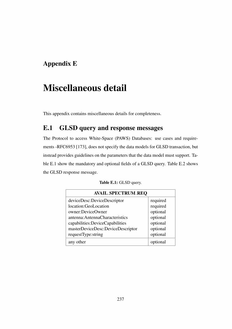
Appendix E

Miscellaneous detail

This appendix contains miscellaneous details for completeness.

E.1 GLSD query and response messagesThe Protocol to access White-Space (PAWS) Databases: use cases and require-

ments -RFC6953 [173], does not specify the data models for GLSD transaction, but

instead provides guidelines on the parameters that the data model must support. Ta-

ble E.1 show the mandatory and optional fields of a GLSD query. Table E.2 shows

the GLSD response message.

Table E.1: GLSD query.

AVAIL SPECTRUM REQdeviceDesc:DeviceDescriptorlocation:GeoLocationowner:DeviceOwnerantenna:AntennaCharacteristicscapabilities:DeviceCapabilitiesmasterDeviceDesc:DeviceDescriptorrequestType:string

requiredrequiredoptionaloptionaloptionaloptionaloptional

any other optional

237

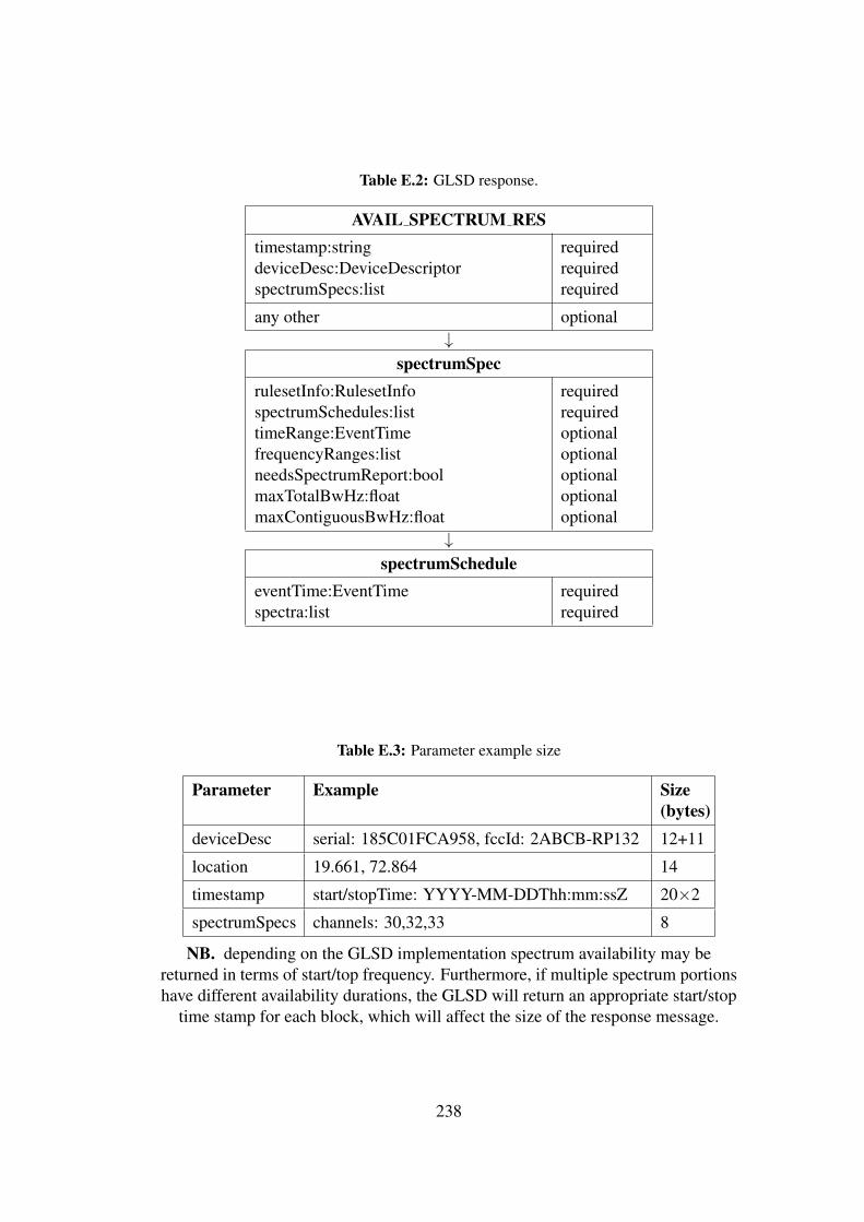
Table E.2: GLSD response.

AVAIL SPECTRUM REStimestamp:stringdeviceDesc:DeviceDescriptorspectrumSpecs:list

requiredrequiredrequired

any other optional↓

spectrumSpecrulesetInfo:RulesetInfospectrumSchedules:listtimeRange:EventTimefrequencyRanges:listneedsSpectrumReport:boolmaxTotalBwHz:floatmaxContiguousBwHz:float

requiredrequiredoptionaloptionaloptionaloptionaloptional

↓spectrumSchedule

eventTime:EventTimespectra:list

requiredrequired

Table E.3: Parameter example size

Parameter Example Size(bytes)

deviceDesc serial: 185C01FCA958, fccId: 2ABCB-RP132 12+11

location 19.661, 72.864 14

timestamp start/stopTime: YYYY-MM-DDThh:mm:ssZ 20×2

spectrumSpecs channels: 30,32,33 8

NB. depending on the GLSD implementation spectrum availability may bereturned in terms of start/top frequency. Furthermore, if multiple spectrum portionshave different availability durations, the GLSD will return an appropriate start/stop

time stamp for each block, which will affect the size of the response message.

238

Appendix F

Reflection

I once heard a story of a millionaire who got asked the question, “how much money

is enough?” His response was, “just a little bit more.”

I liken network performance to money in that the demand for it only increases

with the passage of time. A little bit more improvement in network performance

is always a good idea. This chapter contains snippets of my raw thoughts hovered

over my PhD journey. The tone is less academic, this is intentional.

F.1 Reasoning by analogyI (like most people known to me) think in terms of images. I find it hard to think

about a thing that I do not have a mental picture of. The research road on the other

hand, is riddled with a lot of unknowns, otherwise it would not be called research.

Therefore, to operate in the space of the unknown, I had to locate anchors from the

world I know well to hook the unknown ideas. This parallel mapping of something

unknown to what is known as a scheme of thinking about the unknown occurred

to me quite naturally. It is only later on, further down in my research journey that

I discovered that it is actually a formal method and is referred to as reasoning by

analogy 1. I am now able to look back and say that I applied reasoning by analogy.

Reasoning by analogy is the general principle of accessing knowledge from

analogous fields i.e. drawing inspiration from an analogous field and applying the

1see the article at this url, “Avoiding Superficial” Analogies for the 4-step framework ofreasoning by analogy. https://hbr.org/2005/04/how-strategists-really-think-tapping-the-power-of-analogy?referral=03759&cmvc=rritempage.bottom

239

solution to the target problem as illustrated in Figure F.1. This method of accessing

knowledge from analogous fields has its origins in political science and has since

been applied in business studies. In fact, it has been found that the more distant the

field is from the context of the target problem, the more novel the solution [174]. For

example, several top artificial intelligent algorithms have ironically been inspired by

nature. Notable examples include ant-colony optimisation et al.

Source problem Target problem

Identification: identify the analogy

Analysis: understand the source

Similarity mapping: assess similarity

Application: translate and adapt Target

solutionCandidate solution

Figure F.1: Reasoning by analogy

F.1.1 The price tag

When two or more shops have the item I want, if the items are the same with a rea-

sonable measure of comparison, the obvious thing I do is look at the price tag: the

lowest price always takes the day. The routing metric is a lot like a price tag as the

routing protocol uses it to determine the best path. My experience at the shopping

mall helped me think about the role of the link metric in the routing process more

clearly. Sticking with the price tag metaphor, it follows that if comparisons have

to be made, they can only be made meaningfully if the the prices are quoted in the

same currency. Comparing 13.17 ZAR vs 11.22 ZMK vs 0.82 Euro for instance,

240

is daunting even for the numerically inclined, and nerve-racking when the price tag

is missing altogether! Therefore, a uniform currency should be adopted or there

should be a means of conversion from one currency to the other. As I grappled with

the protocol’s task of deciding between 5 GHz WiFi and UHF-TVWS links, a basic

metric such as packet delivery ratio computed on the two links measures two dif-

ferent things. The challenge indicated struck me as a case of dealing with multiple

currencies. This line of enquiry inspired me to devise the concept of scaling con-

stants (introduced in chapter 5) that are an attempt at an abstract means of levelling

dissimilar quantities.

F.1.2 The delivery guy: inspiration for routing

The “delivery guy” analogy is used in nearly all network fundamentals notes to

illustrate protocol stack mechanics and the movement of data from one device to the

other. As I thought about the routing problem, which is an intangible phenomena, I

had to locate some readily perceivable analogy to tie it to, think with and learn from.

There is obviously plenty analogies to draw from, but the immediate one for me was

a road network, which in many respects is similar to a data communication network.

Considering what a routing protocol does, the protocol and a motor vehicle driver

clearly have similar objectives. I intently observed road traffic on by-ways and

high-ways and the behaviour of road users. Imagining a delivery guy for a busy

courier company on a typical day driving from one point to the other, I personified

the routing protocol and situated it on the passenger’s seat of a delivery van in a bid

to draw lessons from the driver.

Everybody appreciates less or expediate smooth flowing traffic of any kind,

be it road traffic, data traffic, you name it. In this section I try to draw parallels

between the delivery guy and routing by highlighting a few examples out of a long

list of the many ways in which the inner-workings of a routing protocol are similar

to the experience and behaviour of an on-duty delivery driver. At the end of the

day, the whole purpose of reasoning by analogy is to transfer lessons learnt from

well understood processes or phenomena to the target problem area in question.

Inspiration for innovative routing can be drawn from the analogies in the previous

241

paragraph by posing the following metaphorical question: what can the protocol

learn from the delivery guy?

1. Wider/more lanes are better because more cars can pass through at once. In

the context of my work, this equates to spectrum: the wider the operating

channel, the more bits we are able to push into the medium. This is the

ultimate definition of bandwidth. Generally the wider the channel-width, the

better in terms of data transfer. However, going beyond the analogy, there are

several limitations when in reality. Firstly, as the channel-width increases,

transmission distance reduces. Secondly, wider-channel widths are also more

susceptible to noise unless of course there is sufficient investment in perfect

filters.

2. Speed limits, traffic lights, stop signs, time dependency influences how

quickly traffic reaches the destination. Yes the lane is open and oh, there are

other lanes, so multiple vehicles can head-out, but how long it takes to reach

the destination depends on what lies and what happens between the start and

the intended destination. This is akin to throughput, a term that often times

gets confused with bandwidth.

Over time, a driver develops knowledge of the typical road situation based

on time of day. He uses this to determine the best route to take. Spectrum

and network usage are similarly time dependent. In addition to the real-time

mechanism used by the protocol to determine the optimal route, historic data

can be harnessed across two dimensions namely, spectrum usage and network

usage to determine optimal path/channel at a given instance.

3. Smooth road vs pot-hole riddled road is a very good analogy for clear clean

spectrum vs spectrum tainted with unwanted signals. Just as pot-holes force

a good driver to slow down, modulation and coding schemes adjust the data-

rates depending on the quality of spectrum. Generally, when the noise goes

up, the modulation scheme scales down to a lower rate.

4. Changing lanes when and where available, doing it when necessary, and

242

without endangering other motorists is a common sight on the highways and

byways. By observing how motorists utilise the road, I was able to get a grip

on the essence of DSA. It sounds illogical to imagine a road network with a

rule that says, “only this make and colour of vehicle is allowed to ever use a

particular lane.” However, this is exactly what the fixed spectrum assignment

principle has done. It makes sense by all standards for a driver to hop to an

alternative lane when the one they are on gets jammed -and that is what DSA

aims to achieve.

A good driver avoids changing lanes unnecessarily. The driver assess the sit-

uation to determine if the lane is going to be jammed for a significant period

then only does he switch to an alternative lane. If not, he waits patiently for

the lane to clear up again. In the same vein, DSA nodes require mechanisms

to identify the “lanes” to hop into, judge when it is safe to do so and gauge

the potential benefit or cost of switching to an alternative channel. In addi-

tion, there is need to quantify overhead associated with channel switching and

determine key thresholds of when to switch channels.

5. Prioritising is another subroutine I bet the delivery person uses when there

are multiple parcels to deliver and places to go to. I am confident he decides

which one to start with and which one to end with before setting-out. Queuing

packets as and when they arrive at the router and forwarding them based on

first-in-first-out (FIFO) principle works fine and is easy to implement. But,

is there a chance that we might get performance improvement if we build

intelligence into the routers to prioritise traffic and forward accordingly? For

example, routers can give higher priority to traffic generated by applications

with higher real-time constraints such as VoIP traffic and lower priority to

delay tolerant asynchronous data traffic.

6. “No trucks allowed” is a common sign found on byways leading to residen-

tial areas. It is typically there to alert drivers when trucks are not allowed on a

particular road for reasons such as insufficient clearance or optimising traffic

243

flow. On this note, I leave it up to the creative reader to draw lessons from

this and other metaphors and carry on, reasoning by analogy:)

F.2 Design first, model later vs model first, design

later

Over the course of my PhD journey, I found myself engaging in interesting discus-

sions around what the best approach is to this or that. The question was, should a

system be modelled first and then designed or should it be designed first and mod-

elled later?

One might argue that attempting to model what is vaguely understood could

potentially stifle the subsequent design and therefore, we should design first and

model later. However, proponents of the model first, design later approach favour

the approach because the performance of resulting protocols (..and systems in gen-

eral) can automatically be proved analytically. Cesana et al [97] remarked on the

IEEE 802.11 MAC protocol as a case of “design first”, which expectedly lacks an

accurate model particularly for delay.

But what else adds to the confusion, is the disparity in views around what con-

stitutes design particularly within the computer science and computer engineering

fraternity. I head a story of a computer scientist working for a micro-processor

manufacturing company. He described his job as “designing processors”, but his

colleagues with an engineering background corrected him saying, “no, you don’t

design, you draw up processor specifications.”

After a protracted period of soul-searching, considering the arguments for and

against, and analysing it all under the lens of personal experience, I’ve come to the

conclusion that the truth lies somewhere mid-way between model first and design

first. I think that aspects of a system that are well understood can be modelled; the

design itself can add to clarity and conversely inform the modelling.

244

F.3 Progression of ideas

When I started working on this research, my initial set of experiments were con-

ducted to compare the performance of WiFi operating in the 5 GHz and UHF-

TVWS bands. The motive was to determine which one is suitable. However, as it

turned out, there was no clear winner. TVWS performed superiorly in near line-of-

sight whereas, 5 GHz WiFi out-performed TVWS in clear line-of-sight scenarios

at short distances. It was clear at this point that WMN deployments will have to

consist of hybrid links.

The initial idea was to select either 5 GHz or TVWS radio depending on the na-

ture of the signal propagation path. This seemed like a great idea, however I noticed

that throughput in the forward direction was not always equal to the throughput in

the reverse direction. In some instances, the throughput in one direction was nearly

double the throughput in the other direction, which is problematic when deciding

which radio to use. After further experimentation, I observed a common scenario

where one radio had good throughput in say, the forward direction while the other

radio had better throughput in the reverse direction. This pattern begun provoking

ideas about using the radios in concert as a way of mitigating link asymmetry what-

ever the cause might be. This line of enquiry eventually led to the second idea,

which we now refer to as a split link i.e. split a single logical link into two physical

streams e.g. use 5 GHz to transmit and TVWS to receive or vice versa depending on

the nature the asymmetry. The idea is to always try and “put the best foot forward.”

At this stage, the aspirations (if I could call it that) of determining and using the

WINNING radio exclusively had dissipated. The exploration continued to identify

synergies between multiple radios and eventually the idea of aggregating 5 GHz

and TVWS came up i.e. combining 5 GHz and TVWS into a single logical link.

This proved to be beneficial only when the aggregated radios has approximately

uniform data-rates. Armed with General Systems Theory’s assertion that the whole

is greater than the sum of its part, I begun to think critically about how to possibly rip

the benefits of aggregation amid non-uniform data-rates. That is how the Adaptive

Round Robin algorithm detailed in Chapter 6 came about.

245

F.4 Two-ply vs single-ply toilet paperI was in the campus bathroom one day [26 April 2018], it was a Friday and a holiday

in South Africa. I got concerned about the amount of toilet paper that was there

because it being a Friday, the cleaning staff would only replenish the following

Monday. While at it, the thought of two-ply vs one-ply toilet paper came to mind.

It then dawned on me that this is among the many humanity’s unsettled issues as we

continue to find both 2-ply and 1-ply toilet paper on the shelf. The manufacturers

have left the matter up to the end-user to decide and rightly so.

In similar manner, if we regard the choice of whether or not to split/aggregate

hybrid radio links as important as it should be, then I’m inclined to think that the

decision should be made by the nodes. We need to get out of the way and just

ensure the options have the “price tags” well-labelled for nodes to make informed

decisions.

There are two schools of thought. The first one says, while in transit, a parcel

remains the property of the sender. Therefore, the sender should dictate the route

taken by the parcel. This line of thought leads to a conclusion that the split/aggre-

gate decision should be made by the source node. But then again, if we consider

the case of an online shopper, most online retailers let the user choose the shipping

method in which case, the parcel is viewed as belonging more to the recipient than

it does the entity dispatching it. Considering the conventional semantics of source

and destination nodes, this second view leads us to a different conclusion, which

is that the decision rests with the destination node. I consider both arguments to

be valid and I’m of the view that an ideal solution lies somewhere mid-way and is

subject to context.

F.5 Master key, or maybe notWhile conducting the experimental tests, it was important to ensure that the nodes

were operating on the same channel otherwise they would not form a connection.

In between experiments the channel setting would sometimes change and it always

took a moment to figure out why the link wasn’t working. Out of this frustration,

246

it is then that the idea of extending “self-configuring” capabilities to encompass

channel settings came to mind. In the prototyped solution, the node is able to carry

out an exhaustive search of the channel space, detect beacons and set the operating

channel to the channel the beacon was detected on (see Appendix D section D.1 ).

The first limitation is that the detection might take longer as the channel space

enlarges. The other limitation is that though the node is able to auto-configure

its operating channel, its BSSID still has to be configured manually. The BSSID

tells the node which network it belongs to. I thought about automating the BSSID

setting as well, but did not do it. While it might be a desirable feature towards the

realisation of a totally self-configuring network, I did not think it was a wise feature

from a security standpoint. My thinking was, though I would pay both kidneys to

own a key that is capable of opening any door, paradoxically I would fight tooth-

and-nail to avoid having a door that can be opened by any key.

F.6 In the end, everything is virtual

In section 4.2.2 of chapter 4 I talked about virtualisation as a way for single-radio

nodes to deal with a possible shortage in network-wide common channels. The idea

is to use the one radio a node has and create virtual instances to allow the node to

connect to multiple other nodes on different channels as if it had multiple radios.

That is the only portion of my dissertation where I used the term “virtualisation”,

because naturally that is how I understood it at the time.

In retrospect, my finding is that everything is virtual. In a way, virtualisation

can be considered simply as a system of representing resources. With that said, the

kind of virtualisation I presented is what might be termed as 1− to−n i.e. a single

physical entity functionally mapped to multiple instances. I didn’t see it that way

then, but looking back now, the multi-link utilisation approaches presented in chap-

ter 6 can also be considered as virtualisation. For example, radio aggregation can

be said to be virtualisation of the form n− to− 1 i.e. multiple physical resources

(radios) are mapped to a single resource (link) virtually. while other link permuta-

tions may fall in the m− to− n or n− to−m types of virtualisation depending on

247

the number and nature of the mapping between the physical entity and the abstract

instantiations. More detail on that philosophy can be found in Horsman’s article on

Abstract/Representation theory [175].

Now going back to the startling ITU statistics on the world’s offline population

presented in chapter 1 (Figure 1.1), which formed part of the underlying motivation

and fuelled my passion about the research, my answer to the question of “how do

we get the nearly 75% offline population online?”, is one community based network

at a time.

248