PHYSICAL REVIEW E 88, 062707 (2013)

Rheology of a vesicle suspension with finite concentration: A numerical study

Marine Thiebaud* and Chaouqi Misbah†

Laboratoire Interdisciplinaire de Physique/UMR5588, Universite Grenoble I/CNRS, Grenoble F-38041, France(Received 1 August 2013; revised manuscript received 14 October 2013; published 10 December 2013)

Vesicles, closed membranes made of a bilayer of phospholipids, are considered as a biomimetic system forthe mechanics of red blood cells. The understanding of their dynamics under flow and their rheology is expectedto help the understanding of the behavior of blood flow. We conduct numerical simulations of a suspension ofvesicles in two dimensions at a finite concentration in a shear flow imposed by countertranslating rigid boundingwalls by using an appropriate Green’s function. We study the dynamics of vesicles, their spatial configurations,and their rheology, namely, the effective viscosity ηeff . A key parameter is the viscosity contrast λ (the ratiobetween the viscosity of the encapsulated fluid over that of the suspending fluid). For small enough λ, vesiclesare known to exhibit tank treading (TT), while at higher λ they exhibit tumbling (TB). We find that ηeff decreasesin the TT regime, passes a minimum at a critical λ = λc, and increases in the TB regime. This result confirmsprevious theoretical and numerical works performed in the extremely dilute regime, pointing to the robustness ofthe picture even in the presence of hydrodynamic interactions. Our results agree also with very recent numericalsimulations performed in three dimensions both in the dilute and more concentrated regime. This points to the factthat dimensionality does not alter the qualitative features of ηeff . However, they disagree with recent simulationsin two dimensions. We provide arguments about the possible sources of this disagreement.

DOI: 10.1103/PhysRevE.88.062707 PACS number(s): 87.16.D−, 83.80.Lz, 83.60.−a, 47.11.Hj

I. INTRODUCTION

The study of red blood cells (RBCs) and their biomimeticcounterpart (represented by vesicles and capsules) under flowis an essential step towards elucidating a plethora of ques-tions with fundamental, technological, and health interests.Vesicles are closed fluid membranes made of bilayers ofphospholipids, while capsule membranes are made of elasticpolymer networks. These membranes encapsulate a fluid andare suspended in an aqueous solution. Since the modelingof RBCs is rather complex (the modeling of a cytoskeleton,a network of proteins lying beneath the RBC phospholipidbilayer membrane, is still a matter of debate), vesicles andcapsules constitute simpler alternative systems serving as abasis for more elaborate situations. The first system mimicsthe bilayer of the RBC, while the second system mimics theRBC cytoskeleton. From a physical point of view, these threekinds of particles—vesicles, capsules, and RBCs—are mainlycharacterized by their ability to deform (more or less) underflow. Under shear and Poiseuille flows, these particles revealedseveral common varieties of dynamics (see below) [1]. Thesedynamics impact on the suspension rheological behavior.

Since this work is motivated by clarifying the situationabout the rheology of vesicle suspensions at finite concen-trations, a topic that is an ongoing contradictory debate, wefelt it worthwhile to first recall briefly the main steps thatare necessary in order to understand the current state. Undershear flow a vesicle is known to exhibit three basic motions:(i) tank treading (TT), (ii) vacillating breathing (VB) (some-times called trembling or swinging), and (iii) tumbling (TB)motion (see the review in Ref. [1]). The theoretical andnumerical study of the phase diagram of various dynamicsof vesicles under shear flow has shown a significant amount of

*marine.thiebaud@ujf-grenoble.fr†chaouqi.misbah@ujf-grenoble.fr

theoretical, numerical [2–7], and experimental interest [8–10].For a given reduced volume [ν = V/(4π/3)/(A/4π )3/2, whereV and A are the actual vesicle volume and area, respectively],the three kinds of motions can be triggered by increasing theviscosity ratio λ = η1/η0, where η1 is the viscosity of theencapsulated fluid and η0 is the viscosity of the suspendingfluid. More precisely, at low enough λ, vesicles exhibit TT,at high λ TB prevails, while the VB mode takes place atintermediate values of λ.

In the TT regime (with λ small enough) the effectiveviscosity is found to be given by [11,12]

ηeff

η0= 1 + 5

2φ − φ

23λ + 32

16π�, (1)

where � is the excess area from a sphere, related to reducedvolume by � = 4π [ν−2/3 − 1]. The result (1) shows that ηeff

decreases when λ increases, while ηeff increases with λ for anemulsion, as predicted by Taylor [13]. An extensive physicaldiscussion of this difference between emulsion and vesiclesuspensions can be found in Ref. [14]. Relation (1) is validin the TT regime. By increasing λ, there is a critical value λc

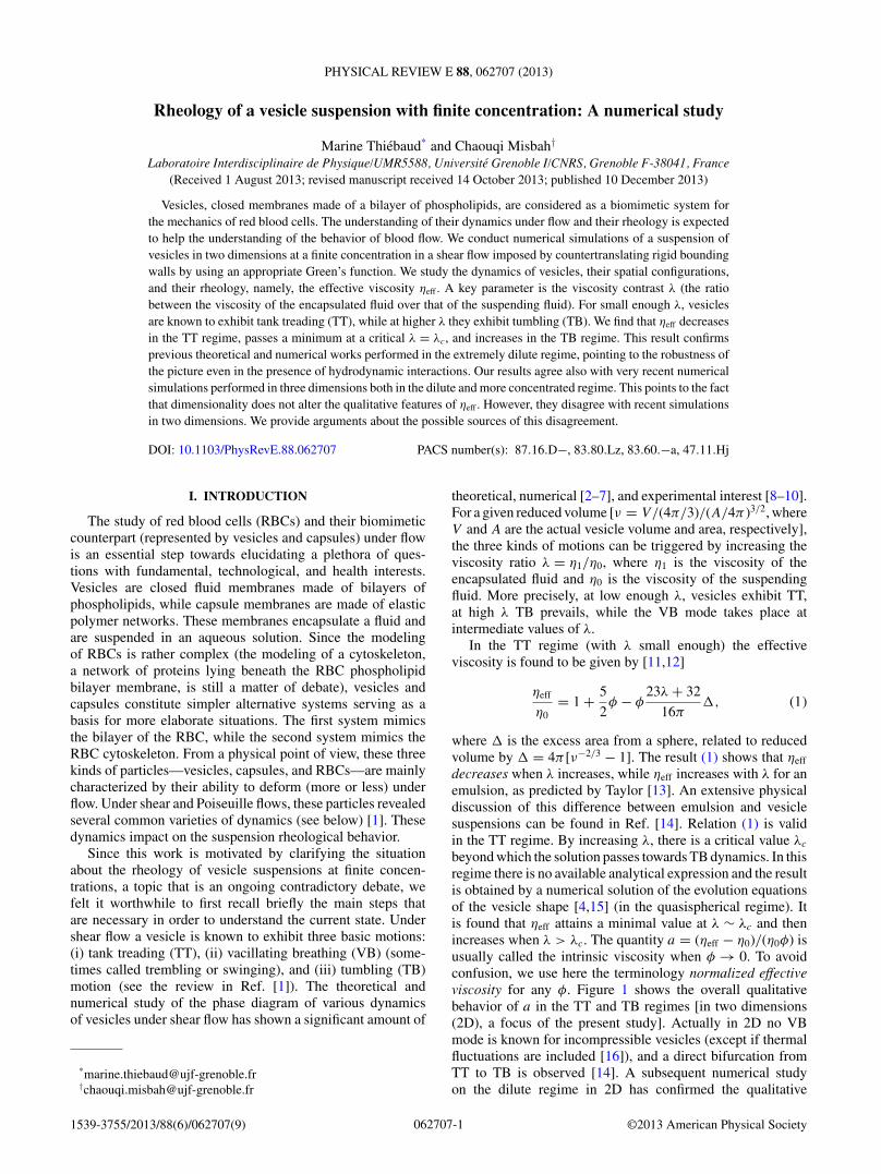
beyond which the solution passes towards TB dynamics. In thisregime there is no available analytical expression and the resultis obtained by a numerical solution of the evolution equationsof the vesicle shape [4,15] (in the quasispherical regime). Itis found that ηeff attains a minimal value at λ ∼ λc and thenincreases when λ > λc. The quantity a = (ηeff − η0)/(η0φ) isusually called the intrinsic viscosity when φ → 0. To avoidconfusion, we use here the terminology normalized effectiveviscosity for any φ. Figure 1 shows the overall qualitativebehavior of a in the TT and TB regimes [in two dimensions(2D), a focus of the present study]. Actually in 2D no VBmode is known for incompressible vesicles (except if thermalfluctuations are included [16]), and a direct bifurcation fromTT to TB is observed [14]. A subsequent numerical studyon the dilute regime in 2D has confirmed the qualitative

062707-11539-3755/2013/88(6)/062707(9) ©2013 American Physical Society

MARINE THIEBAUD AND CHAOUQI MISBAH PHYSICAL REVIEW E 88, 062707 (2013)

FIG. 1. (Color online) Figure adapted from Ghilgliotti [23].Illustration of the typical behavior of the normalized effectiveviscosity as a function of the viscosity contrast obtained by thetwo-dimensional numerical simulation of Ghigliotti et al. [14]. Inthe TT regime the viscosity decreases, while it increases in the TBregime.

features of Fig. 1 beyond the small deformation theory (i.e.,for vesicles whose shape is far from a circle [14]). The sameconclusion was reached numerically for a dilute suspension inthree dimensions (3D) by Rahimian et al. [17]. A similar trendhas also been observed for capsules using a 3D simulation [18].The question of how would the above results (especially thequalitative behavior in Fig. 1) evolve beyond the dilute regimewas left open.

Studies at finite vesicle concentrations have been performedrecently by two groups. The first work [19] (in 3D) confirmsthe trend shown in Fig. 1, while the second work (in 2D)contradicts it [20]. Table I summarizes the behavior of a (last

column) obtained by different groups both in the dilute andmore concentrated regimes. The descending (ascending) arrowindicates decreasing (increasing) viscosity.

Two series of experiments have been undertaken by twodifferent groups (Vitkova et al. [21] and Kantsler et al. [22])in order to study ηeff as a function of λ. These two groupsdisagree with each other, as summarized in Table I. All thenumerical works (see Table I), except that of Lamura andGompper, agree (at least qualitatively) with the experiments ofVitkova et al. [21] that were performed on vesicles and RBCs.Only the numerical study of Lamura and Gompper partiallyagrees (at small λ, where a increases with λ; see Table I) withthe experiments of Kantsler et al. [22]. A possible source forthe explanation of the contradiction of the results of Lamuraand Gompper [20] with all other numerical studies might beattributed to thermal fluctuations (which are inherently presentin their method). We shall come back to this issue in thediscussion section of this paper.

Given this unclear situation, the question naturally arisesas to whether one could understand the difference in theresults obtained at a finite concentration in 3D by Zhaoet al. [19] (using periodic boundary conditions in all the threedirections of space) and that of Lamura and Gompper [20]obtained in 2D (using rigid walls but periodic boundaryconditions along the flow direction). The following naturalquestions have guided the present study: (i) Is the differ-ence attributed to dimensionality? (ii) Is this due to theboundary conditions? (iii) Is there a hidden reason for thisdiscrepancy?

We have conducted 2D simulations by using the sameboundary conditions and the same parameter range as Lamuraand Gompper [20]. Our results are found to be qualitativelydifferent from those of Lamura and Gompper [20]: We finda nonmonotonous behavior of a, in accord with the generaltrend shown in Fig. 1.

TABLE I. Summary of different results of vesicle and red blood cell suspension rheology. Different abbreviations are used: RBC for redblood cells, Ves. for vesicle, 3D for three dimensions, 2D for two dimensions, expt. for experiments, simul. for simulations, φ is the area orvolume fraction according to whether the space dimension is 2D or 3D, γ is the shear rate, and Cκ (defined below in the main text) is thecapillary number, the ratio between the shear rate and the vesicle shape relaxation time.

Article Type φ ν Flow strength λc Behavior of a as function of λ

Vitkova et al. [21] RBC, 3D, expt. 5%, 7.5% 0.6 γ ∼ 100 s−1 ∼1–3 0.1 ↘ λc ∼ 1–3 ↗ 20

Vitkova et al. [21] Ves., 3D, expt.From 2.5%

to 12%0.9–1 γ ∼ 100 s−1 ∼3 0.1 ↘ λc ∼ 3 ↗ 10

Kanstler et al. [22] Ves., 3D, expt. 11.3% 0.93–0.98γ from

1 to 50 s −1 ∼8–9 0.1 ↗∼ 1 ↘λc ∼ 8–9 ↘10

Ghigliotti et al. [14] Ves., 2D, simul. 0% 0.7–0.95 Cκ = 13.8 for ν = 0.77 for ν = 0.95

0.1 ↘ λc ↗ 200

Rahimian et al. [17] Ves., 2D, simul. 0%0.6,0.75,

and 0.9Cκ = 1 4.1 for ν = 0.75 0.1↘ ∼ 3 for ν = 0.6

∼ 5 for ν = 0.9↗ 10

Lamura et al. [20] Ves., 2D, simul.5%,9%,

and 14%0.8 Cκ ∼ 2 ∼3.7 1 ↗ λc ∼ 3.7 ↗ 10

Zhao et al. [19] Ves., 3D, simul.From 5%to 20%

0.95 Cκ = 18.46 at φ = 0%λc ↗ with φ

0.1 ↘ 7 for φ = 0%10 for φ = 20%

↗14

Current work Ves., 2D, simul. 0% and 6.21% 0.7 Cκ = 1 ∼11 0.1 ↘ λc ↗100

062707-2

RHEOLOGY OF A VESICLE SUSPENSION WITH FINITE . . . PHYSICAL REVIEW E 88, 062707 (2013)

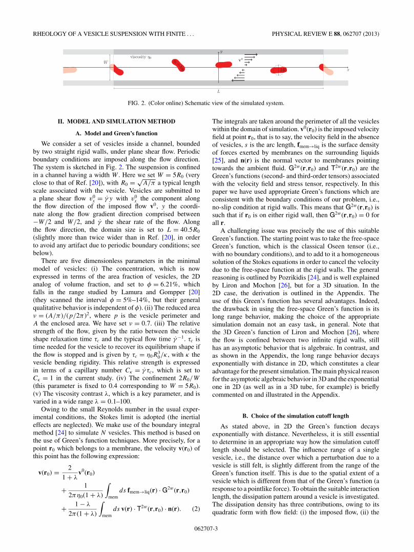
FIG. 2. (Color online) Schematic view of the simulated system.

II. MODEL AND SIMULATION METHOD

A. Model and Green’s function

We consider a set of vesicles inside a channel, boundedby two straight rigid walls, under plane shear flow. Periodicboundary conditions are imposed along the flow direction.The system is sketched in Fig. 2. The suspension is confinedin a channel having a width W . Here we set W = 5R0 (veryclose to that of Ref. [20]), with R0 = √

A/π a typical lengthscale associated with the vesicle. Vesicles are submitted toa plane shear flow v0

x = γ y with v0x the component along

the flow direction of the imposed flow v0, y the coordi-nate along the flow gradient direction comprised between−W/2 and W/2, and γ the shear rate of the flow. Alongthe flow direction, the domain size is set to L = 40.5R0

(slightly more than twice wider than in Ref. [20], in orderto avoid any artifact due to periodic boundary conditions; seebelow).

There are five dimensionless parameters in the minimalmodel of vesicles: (i) The concentration, which is nowexpressed in terms of the area fraction of vesicles, the 2Danalog of volume fraction, and set to φ = 6.21%, whichfalls in the range studied by Lamura and Gompper [20](they scanned the interval φ = 5%–14%, but their generalqualitative behavior is independent of φ). (ii) The reduced areaν = (A/π )/(p/2π )2, where p is the vesicle perimeter andA the enclosed area. We have set ν = 0.7. (iii) The relativestrength of the flow, given by the ratio between the vesicleshape relaxation time τc and the typical flow time γ −1. τc istime needed for the vesicle to recover its equilibrium shape ifthe flow is stopped and is given by τc = η0R

30/κ , with κ the

vesicle bending rigidity. This relative strength is expressedin terms of a capillary number Cκ = γ τc, which is set toCκ = 1 in the current study. (iv) The confinement 2R0/W

(this parameter is fixed to 0.4 corresponding to W = 5R0).(v) The viscosity contrast λ, which is a key parameter, and isvaried in a wide range λ = 0.1–100.

Owing to the small Reynolds number in the usual exper-imental conditions, the Stokes limit is adopted (the inertialeffects are neglected). We make use of the boundary integralmethod [24] to simulate N vesicles. This method is based onthe use of Green’s function techniques. More precisely, for apoint r0 which belongs to a membrane, the velocity v(r0) ofthis point has the following expression:

v(r0) = 2

1 + λv0(r0)

+ 1

2πη0(1 + λ)

∫mem

ds fmem→liq(r) · G2w(r,r0)

+ 1 − λ

2π (1 + λ)

∫mem

ds v(r) · T2w(r,r0) · n(r). (2)

The integrals are taken around the perimeter of all the vesicleswithin the domain of simulation. v0(r0) is the imposed velocityfield at point r0, that is to say, the velocity field in the absenceof vesicles, s is the arc length, fmem→liq is the surface densityof forces exerted by membranes on the surrounding liquids[25], and n(r) is the normal vector to membranes pointingtowards the ambient fluid. G2w(r,r0) and T2w(r,r0) are theGreen’s functions (second- and third-order tensors) associatedwith the velocity field and stress tensor, respectively. In thispaper we have used appropriate Green’s functions which areconsistent with the boundary conditions of our problem, i.e.,no-slip condition at rigid walls. This means that G2w(r,r0) issuch that if r0 is on either rigid wall, then G2w(r,r0) = 0 forall r.

A challenging issue was precisely the use of this suitableGreen’s function. The starting point was to take the free-spaceGreen’s function, which is the classical Oseen tensor (i.e.,with no boundary conditions), and to add to it a homogeneoussolution of the Stokes equations in order to cancel the velocitydue to the free-space function at the rigid walls. The generalreasoning is outlined by Pozrikidis [24], and is well explainedby Liron and Mochon [26], but for a 3D situation. In the2D case, the derivation is outlined in the Appendix. Theuse of this Green’s function has several advantages. Indeed,the drawback in using the free-space Green’s function is itslong range behavior, making the choice of the appropriatesimulation domain not an easy task, in general. Note thatthe 3D Green’s function of Liron and Mochon [26], wherethe flow is confined between two infinite rigid walls, stillhas an asymptotic behavior that is algebraic. In contrast, andas shown in the Appendix, the long range behavior decaysexponentially with distance in 2D, which constitutes a clearadvantage for the present simulation. The main physical reasonfor the asymptotic algebraic behavior in 3D and the exponentialone in 2D (as well as in a 3D tube, for example) is brieflycommented on and illustrated in the Appendix.

B. Choice of the simulation cutoff length

As stated above, in 2D the Green’s function decaysexponentially with distance. Nevertheless, it is still essentialto determine in an appropriate way how the simulation cutofflength should be selected. The influence range of a singlevesicle, i.e., the distance over which a perturbation due to avesicle is still felt, is slightly different from the range of theGreen’s function itself. This is due to the spatial extent of avesicle which is different from that of the Green’s function (aresponse to a pointlike force). To obtain the suitable interactionlength, the dissipation pattern around a vesicle is investigated.The dissipation density has three contributions, owing to itsquadratic form with flow field: (i) the imposed flow, (ii) the

062707-3

MARINE THIEBAUD AND CHAOUQI MISBAH PHYSICAL REVIEW E 88, 062707 (2013)

FIG. 3. (Color online) Surface density of dissipation in dimensionless units (the three fundamental units are R0, τc, and the viscosity η0)around one vesicle. The abscissa is the coordinate along the flow direction counted from the center of mass of the vesicle. The y axis is thecoordinate along the flow gradient direction. The dissipation is maximum near walls. To define the influence range of a vesicle, we plot ina solid black bold curve the absolute value of the density of dissipation near one wall (taken here to be the lower one) as a function of thedistance from the vesicle center of mass along the flow direction. The right y axis is used as a log scale for the absolute value of dissipation.The dotted straight lines represent the envelopes of dissipation which cross the x axis at about x = ±16.2. The vertical black bold line is theborder beyond which the vesicle influence is negligible, according to our numerical tolerance.

coupling between the imposed flow and the additional flowinduced by the vesicle, and (iii) the purely induced flow dueto the vesicle. Only the last two terms matter regarding theinfluence of a vesicle, and their sum is shown in Fig. 3. As adifference of two positive terms, this sum may be positive ornegative. The dissipation is the largest in the vesicle vicinity,but is also quite large in the vicinity of the walls. We havefound that far away from the vesicle, in the x direction,dissipation is the highest in the wall vicinity, so that we takethis quantity in order to characterize the influence range of avesicle. This influence range is not visible in the color codeused in Fig. 3. Therefore we have represented (black boldcurve) the logarithm of the absolute value of the dissipationdensity near the lower wall (which is similar to that nearthe upper wall), with the magnitude shown on the right sideof the simulation box. The dotted line is the envelope ofthe dissipation function, and our criterion is that the vesicleinfluence is vanishingly small when the envelope crosses zero.This occurs at about x � ±16.2R0 from the center of thevesicle. Thus the distance between the centers of two vesicles,one in the simulation domain and the other in one of thetwo fictitious boxes (obtained by periodic condition on theright and left of the considered domain), must be separated byabout twice the above distance. Setting the simulation domainL = 40.5R0 guarantees safely our demand for mimicking aninfinite domain.

III. RESULTS

A. Vesicle spatiotemporal configurations

The first task is to investigate the spatial configurationsof the suspension for different viscosity contrasts. The simu-lations are run for a long enough time in order to ascertainnot only that the transients have decayed, but also that afirm permanent regime is attained. The memory of “initialconfigurations” is lost quite rapidly due to lift motions awayfrom the walls [27–29], and to hydrodynamic diffusion due tointeractions among the vesicles [30]. The final configurationsare presented in Fig. 4 for various viscosity contrasts. Atrelatively small viscosity contrast, λ � 10, that is to say, inthe TT regime, the lift force caused by the walls inducesvesicles centering in the channel. The final distribution is quitehomogeneous. However, at a larger viscosity contrast λ > 10,in the TB regime, the spatiotemporal evolution of the vesicleconfigurations presents a complex dynamics that looks rather

chaotic. The spatiotemporal configurations have an impact onthe overall rheological properties.

B. Instantaneous rheology

From a macroscopic point of view, suspensions are charac-terized by rheological quantities, such as the effective viscosityor normal stress difference. The effective viscosity quantifiesthe resistance of the suspension to an imposed flow. Moreprecisely, in a plane shear flow,

ηeff = 〈σxy〉γ

= 〈σyx〉γ

, (3)

where brackets 〈· · · 〉 denote a surface average (2D analogof volume average), γ is the shear rate, and σ is the totalstress tensor within the suspension. σ has two contributions:the solvent and vesicle contributions. The above definition isan intuitive one: It is the ratio between the required force toobtain an imposed flow with the desired shear rate. Whiledefinition (3) looks similar to that of usual simple fluids, thereis a hidden important difference carried by the average symbol.Indeed, while for simple fluids (such as water) the stress andstrain rate are homogeneous in space within the gap and aretime independent, this is not the case here since vesicles maychange position and orientation in the course of macroscopictime imposed by the external shear flow. Thus, the stressand strain rate change over the course of time (implying thatviscosity is also time dependent), and one has to average overmany space and time configurations. This is why we adopt the

W

L

(a)

(b)

(c)

(d)

(e)

FIG. 4. (Color online) Typical configurations at late time for fourvesicles in a shear flow confined in a channel whose height is W =5R0 for several viscosity contrasts: (a) λ = 1, (b) λ = 5, (c) λ = 10,(d) λ = 50, and (e) λ = 100.

062707-4

RHEOLOGY OF A VESICLE SUSPENSION WITH FINITE . . . PHYSICAL REVIEW E 88, 062707 (2013)

1.6 1.8

2 2.2 2.4 λ=1

1.5 1.7 1.9 λ=5

1.6 2

2.4

inst

anta

neou

s nor

mal

ized

eff

ectiv

e vi

scos

ity

λ=10

2 4 6 λ=50

2

4

6

0 100 200 300 400 500 600 700time (in units of τc)

λ=100

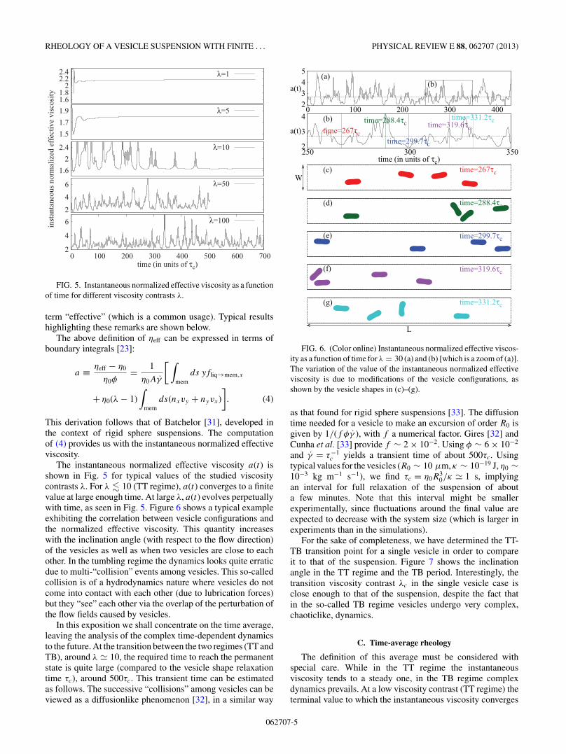
FIG. 5. Instantaneous normalized effective viscosity as a functionof time for different viscosity contrasts λ.

term “effective” (which is a common usage). Typical resultshighlighting these remarks are shown below.

The above definition of ηeff can be expressed in terms ofboundary integrals [23]:

a ≡ ηeff − η0

η0φ= 1

η0Aγ

[ ∫mem

ds yfliq→mem,x

+ η0(λ − 1)∫

memds(nxvy + nyvx)

]. (4)

This derivation follows that of Batchelor [31], developed inthe context of rigid sphere suspensions. The computationof (4) provides us with the instantaneous normalized effectiveviscosity.

The instantaneous normalized effective viscosity a(t) isshown in Fig. 5 for typical values of the studied viscositycontrasts λ. For λ � 10 (TT regime), a(t) converges to a finitevalue at large enough time. At large λ, a(t) evolves perpetuallywith time, as seen in Fig. 5. Figure 6 shows a typical exampleexhibiting the correlation between vesicle configurations andthe normalized effective viscosity. This quantity increaseswith the inclination angle (with respect to the flow direction)of the vesicles as well as when two vesicles are close to eachother. In the tumbling regime the dynamics looks quite erraticdue to multi-“collision” events among vesicles. This so-calledcollision is of a hydrodynamics nature where vesicles do notcome into contact with each other (due to lubrication forces)but they “see” each other via the overlap of the perturbation ofthe flow fields caused by vesicles.

In this exposition we shall concentrate on the time average,leaving the analysis of the complex time-dependent dynamicsto the future. At the transition between the two regimes (TT andTB), around λ � 10, the required time to reach the permanentstate is quite large (compared to the vesicle shape relaxationtime τc), around 500τc. This transient time can be estimatedas follows. The successive “collisions” among vesicles can beviewed as a diffusionlike phenomenon [32], in a similar way

2 3 4 5

0 100 200 300 400

a(t)(a)

(b)

2

3

4

250 300 350

a(t)

time (in units of τc)

(b)time=267τc

time=288.4τc

time=299.7τc

time=319.6τctime=331.2τc

W(c) time=267τc

(d) time=288.4τc

(e) time=299.7τc

(f) time=319.6τc

(g)

L

time=331.2τc

FIG. 6. (Color online) Instantaneous normalized effective viscos-ity as a function of time for λ = 30 (a) and (b) [which is a zoom of (a)].The variation of the value of the instantaneous normalized effectiveviscosity is due to modifications of the vesicle configurations, asshown by the vesicle shapes in (c)–(g).

as that found for rigid sphere suspensions [33]. The diffusiontime needed for a vesicle to make an excursion of order R0 isgiven by 1/(f φγ ), with f a numerical factor. Gires [32] andCunha et al. [33] provide f ∼ 2 × 10−2. Using φ ∼ 6 × 10−2

and γ = τ−1c yields a transient time of about 500τc. Using

typical values for the vesicles (R0 ∼ 10 μm, κ ∼ 10−19 J, η0 ∼10−3 kg m−1 s−1), we find τc = η0R

30/κ � 1 s, implying

an interval for full relaxation of the suspension of abouta few minutes. Note that this interval might be smallerexperimentally, since fluctuations around the final value areexpected to decrease with the system size (which is larger inexperiments than in the simulations).

For the sake of completeness, we have determined the TT-TB transition point for a single vesicle in order to compareit to that of the suspension. Figure 7 shows the inclinationangle in the TT regime and the TB period. Interestingly, thetransition viscosity contrast λc in the single vesicle case isclose enough to that of the suspension, despite the fact thatin the so-called TB regime vesicles undergo very complex,chaoticlike, dynamics.

C. Time-average rheology

The definition of this average must be considered withspecial care. While in the TT regime the instantaneousviscosity tends to a steady one, in the TB regime complexdynamics prevails. At a low viscosity contrast (TT regime) theterminal value to which the instantaneous viscosity converges

062707-5

MARINE THIEBAUD AND CHAOUQI MISBAH PHYSICAL REVIEW E 88, 062707 (2013)

0

5

10

15

20

25

0.1 1 10 100 0

5

10

15

20

25

30

incl

inat

ion

(in º)

perio

d tim

e (in

uni

ts o

f τc)

λ

Tank-treadingregime

Tumblingregime

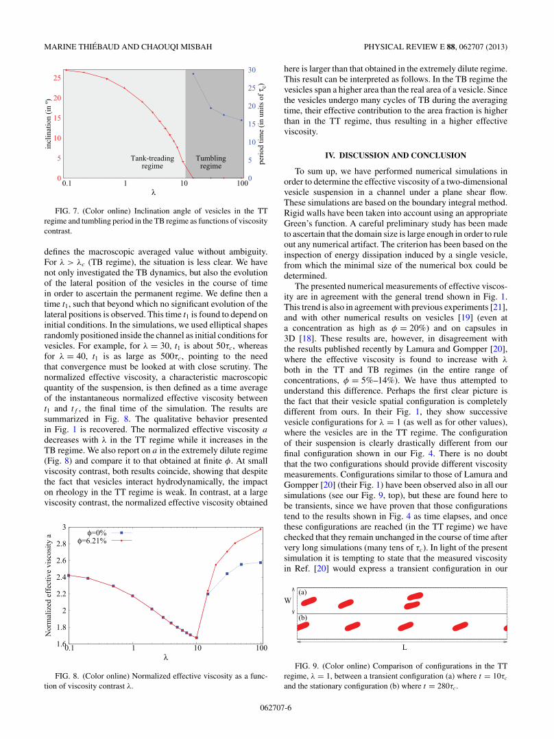
FIG. 7. (Color online) Inclination angle of vesicles in the TTregime and tumbling period in the TB regime as functions of viscositycontrast.

defines the macroscopic averaged value without ambiguity.For λ > λc (TB regime), the situation is less clear. We havenot only investigated the TB dynamics, but also the evolutionof the lateral position of the vesicles in the course of timein order to ascertain the permanent regime. We define then atime t1, such that beyond which no significant evolution of thelateral positions is observed. This time t1 is found to depend oninitial conditions. In the simulations, we used elliptical shapesrandomly positioned inside the channel as initial conditions forvesicles. For example, for λ = 30, t1 is about 50τc, whereasfor λ = 40, t1 is as large as 500τc, pointing to the needthat convergence must be looked at with close scrutiny. Thenormalized effective viscosity, a characteristic macroscopicquantity of the suspension, is then defined as a time averageof the instantaneous normalized effective viscosity betweent1 and tf , the final time of the simulation. The results aresummarized in Fig. 8. The qualitative behavior presentedin Fig. 1 is recovered. The normalized effective viscosity a

decreases with λ in the TT regime while it increases in theTB regime. We also report on a in the extremely dilute regime(Fig. 8) and compare it to that obtained at finite φ. At smallviscosity contrast, both results coincide, showing that despitethe fact that vesicles interact hydrodynamically, the impacton rheology in the TT regime is weak. In contrast, at a largeviscosity contrast, the normalized effective viscosity obtained

1.6

1.8

2

2.2

2.4

2.6

2.8

3

0.1 1 10 100

Nor

mal

ized

eff

ectiv

e vi

scos

ity a

λ

φ=0%φ=6.21%

FIG. 8. (Color online) Normalized effective viscosity as a func-tion of viscosity contrast λ.

here is larger than that obtained in the extremely dilute regime.This result can be interpreted as follows. In the TB regime thevesicles span a higher area than the real area of a vesicle. Sincethe vesicles undergo many cycles of TB during the averagingtime, their effective contribution to the area fraction is higherthan in the TT regime, thus resulting in a higher effectiveviscosity.

IV. DISCUSSION AND CONCLUSION

To sum up, we have performed numerical simulations inorder to determine the effective viscosity of a two-dimensionalvesicle suspension in a channel under a plane shear flow.These simulations are based on the boundary integral method.Rigid walls have been taken into account using an appropriateGreen’s function. A careful preliminary study has been madeto ascertain that the domain size is large enough in order to ruleout any numerical artifact. The criterion has been based on theinspection of energy dissipation induced by a single vesicle,from which the minimal size of the numerical box could bedetermined.

The presented numerical measurements of effective viscos-ity are in agreement with the general trend shown in Fig. 1.This trend is also in agreement with previous experiments [21],and with other numerical results on vesicles [19] (even ata concentration as high as φ = 20%) and on capsules in3D [18]. These results are, however, in disagreement withthe results published recently by Lamura and Gompper [20],where the effective viscosity is found to increase with λ

both in the TT and TB regimes (in the entire range ofconcentrations, φ = 5%–14%). We have thus attempted tounderstand this difference. Perhaps the first clear picture isthe fact that their vesicle spatial configuration is completelydifferent from ours. In their Fig. 1, they show successivevesicle configurations for λ = 1 (as well as for other values),where the vesicles are in the TT regime. The configurationof their suspension is clearly drastically different from ourfinal configuration shown in our Fig. 4. There is no doubtthat the two configurations should provide different viscositymeasurements. Configurations similar to those of Lamura andGompper [20] (their Fig. 1) have been observed also in all oursimulations (see our Fig. 9, top), but these are found here tobe transients, since we have proven that those configurationstend to the results shown in Fig. 4 as time elapses, and oncethese configurations are reached (in the TT regime) we havechecked that they remain unchanged in the course of time aftervery long simulations (many tens of τc). In light of the presentsimulation it is tempting to state that the measured viscosityin Ref. [20] would express a transient configuration in our

W

L

(a)

(b)

FIG. 9. (Color online) Comparison of configurations in the TTregime, λ = 1, between a transient configuration (a) where t = 10τc

and the stationary configuration (b) where t = 280τc.

062707-6

RHEOLOGY OF A VESICLE SUSPENSION WITH FINITE . . . PHYSICAL REVIEW E 88, 062707 (2013)

study. Another important difference between the two groupsis the following. Their system size along the flow direction istaken to be 18.95R0, a value around which we still observeperiodicity artifacts (a vesicle feels its own influence but alsothe influence of its twin located one period before and/or after).We have seen here, by analyzing the influence range due to avesicle, that the box size must be taken equal to, or larger than,36R0 in order to avoid artificial contributions.

Another possible source for the disagreement is that inthe numerical method of Ref. [20] thermal fluctuations areinherently present (due to the very nature of the methodused), so that the question naturally arises as to how thatwould affect the rheological properties. In the experimentsof Levant et al. [34] it is reported that thermal fluctuations ofthe vesicle membrane are important. In addition to membranefluctuations one may also think that fluctuations may induceBrownian diffusion of the center of mass of the vesicle, sothat vesicles may exhibit lateral excursions in the channel.In this way the spatial configurations of the suspension maydiffer from ours, and could explain the difference betweenthe present results and those of Lamura and Gompper [20].In the presence of shear flow the energy injected in thevesicle motion is of the order of η0γ R3

0, to be compared tothermal energy kBT . The fluctuation of the center of massis relevant if R0 < [kBT /(η0γ )]1/3. Using typical values ofdifferent parameters, one finds R0 < 1 μm, which is smallas compared to the usual sizes of the vesicles investigatedexperimentally [21,22]. We have to keep in mind, however, thatthis is just a rough estimate which requires further refinement.It would be an interesting task for future investigations toanalyze numerically the behavior of rheology by increasingprogressively the amplitude of noise. This will enable us to seewhether or not there exists, upon increasing noise strength, atransition (or crossover) between the behavior reported hereand that found in Ref. [20].

Finally, a relevant question concerns the determination ofthe concentration value beyond which hydrodynamic interac-tions among vesicles play a role. In a recent experiment [35]it has been reported that this value is of about 8%–13%.This value depends on various parameters such as viscositycontrast λ, as shown here, where hydrodynamic interactionsare negligible in the TT regime but not in the TB regime, evenfor φ � 6%.

ACKNOWLEDGMENT

We acknowledge financial support from CNES (Centred’Etudes Spatiales) and ESA (European Space Agency).

APPENDIX: OBTENTION OF THE 2D GREEN’SFUNCTIONS IN A CONFINED GEOMETRY

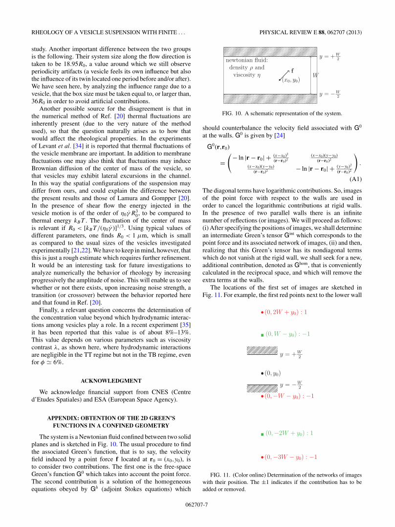
The system is a Newtonian fluid confined between two solidplanes and is sketched in Fig. 10. The usual procedure to findthe associated Green’s function, that is to say, the velocityfield induced by a point force f located at r0 = (x0,y0), isto consider two contributions. The first one is the free-spaceGreen’s function G0 which takes into account the point force.The second contribution is a solution of the homogeneousequations obeyed by Gh (adjoint Stokes equations) which

y = −W2

y = +W2

(x0, y0)

f

newtonian fluid:density ρ and

viscosity η W

FIG. 10. A schematic representation of the system.

should counterbalance the velocity field associated with G0

at the walls. G0 is given by [24]

G0(r,r0)

=(

− ln |r − r0| + (x−x0)2

(r−r0)2(x−x0)(y−y0)

(r−r0)2

(x−x0)(y−y0)(r−r0)2 − ln |r − r0| + (y−y0)2

(r−r0)2

).

(A1)

The diagonal terms have logarithmic contributions. So, imagesof the point force with respect to the walls are used inorder to cancel the logarithmic contributions at rigid walls.In the presence of two parallel walls there is an infinitenumber of reflections (or images). We will proceed as follows:(i) After specifying the positions of images, we shall determinean intermediate Green’s tensor Gint which corresponds to thepoint force and its associated network of images, (ii) and then,realizing that this Green’s tensor has its nondiagonal termswhich do not vanish at the rigid wall, we shall seek for a new,additional contribution, denoted as Ghom, that is convenientlycalculated in the reciprocal space, and which will remove theextra terms at the walls.

The locations of the first set of images are sketched inFig. 11. For example, the first red points next to the lower wall

y = −W2

y = +W2

(0, y0)

(0,−W − y0) : −1

(0, 2W + y0) : 1

(0,−3W − y0) : −1

(0, W − y0) : −1

(0,−2W + y0) : 1

FIG. 11. (Color online) Determination of the networks of imageswith their position. The ±1 indicates if the contribution has to beadded or removed.

062707-7

MARINE THIEBAUD AND CHAOUQI MISBAH PHYSICAL REVIEW E 88, 062707 (2013)

in Fig. 11 designate the reflections of the point force (inside thephysical domain) by the lower wall. The determination of itsfirst image will cancel the diagonal contributions at the lowerwall but not at the upper wall, so that the image of this firstimage with respect to the upper wall is to be considered, and soon. The first green square next to the upper wall represents inFig. 11 the reflection of the (physical) point force by the upperwall. To sum up, the obtained Green’s function correspondingto these series of images, which we shall call the intermediate(for reasons that will become clear below) Green’s functionGint, is the sum over two infinite sets of images (red and green)that add up with alternating signs of forces.

Without loss of generality, we can take the abscissa of r0 asthe origin. After summations over the above-mentioned setsof images, one finds

Gint(x,y; 0,y0) =+∞∑

k=−∞G0(x,y; 0,2Wk + y0)

−+∞∑

k=−∞G0(x,y; 0,2Wk + W − y0)

= G(

xW

,y−y0

W

) − G(

xW

,y+y0−W

W

)2

, (A2)

with

G(x,y)

=(

(− ln[f (x,y)] + g(x,y)) h(x,y)

h(x,y) (− ln[f (x,y)] − g(x,y))

),

where f (x,y) = cosh(πx)− cos(πy), g(x,y)=(πx) sinh(πx)/f (x,y), and h(x,y) = (πx) sin(πy)/f (x,y). At the rigid wallswe have

Gintxy

(x,

W

2; 0,y0

)= Gint

yx

(x,

W

2; 0,y0

)

= πx

W

cos(πy0/W )

cosh(πx/W ) − sin(πy0/W ),

(A3)

Gintxy

(x,−W

2; 0,y0

)= Gint

yx

(x,−W

2; 0,y0

)

= −πx

W

cos(πy0/W )

cosh(πx/W ) + sin(πy0/W ),

(A4)

while diagonal terms vanish exactly on the walls.Because of the nonzero, nondiagonal terms at the walls, Gint

is not sufficient to take into account the channel geometry. Anadditional tensor has to be added in order to fulfill the requiredboundary conditions. To calculate this supplementary tensor,denoted by Ghom, it is convenient to use the reciprocal space.As usual, direct and inverse Fourier transforms are defined as

fk =∫ +∞

−∞dxf exp(−ikx), f =

∫ +∞

−∞

dk

2πfk exp(ikx),

(A5)

-0.5

0

0.5

-1 -0.5 0 0.5 1

(a)

-0.5

0

0.5

-1 -0.5 0 0.5 1

(b)

-0.5

0

0.5

-1 -0.5 0 0.5 1

(c)

-0.5

0

0.5

-1 -0.5 0 0.5 1

(d)

FIG. 12. (Color online) Representation of the velocity Green’sfunctions (black arrows) with corresponding point forces (redarrows): without boundary by using “infinite” Green’s functions (a)and (b). In (c) and (d) the velocity field with suitable boundaryconditions [G2w(r,r0)] is represented. We consider in both cases (a),(c) horizontal and (b), (d) vertical forces. Lengths are counted inunits of channel width, the only length scale; because we comparetwo different Green’s functions, they should both be rescaled by thesame length. Despite the fact that the infinite Green’s function has nointrinsic length scale, we are still at liberty to count the distance inunits of W .

where f stands for any components of the Green’s tensors. Asolution in Fourier space of the homogeneous equation obeyedby Ghom and fulfilling the appropriate boundary conditions canbe evaluated in a straightforward manner. We list below onecomponent of the sought after contribution of the Green’s

-20

-10

0

10

20

-20 -10 0 10 20

z (in

uni

ts o

f W)

x (in units of W)10-3

10-2

10-1

100

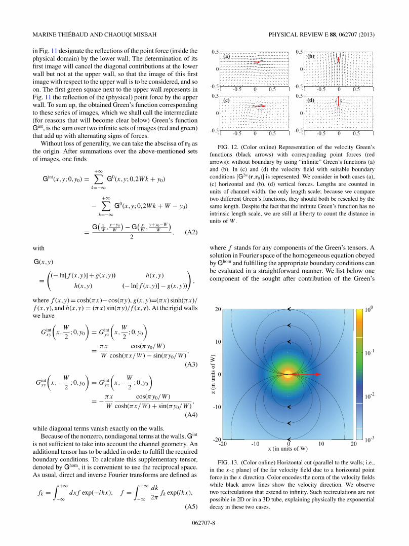
FIG. 13. (Color online) Horizontal cut (parallel to the walls; i.e.,in the x-z plane) of the far velocity field due to a horizontal pointforce in the x direction. Color encodes the norm of the velocity fieldswhile black arrow lines show the velocity direction. We observetwo recirculations that extend to infinity. Such recirculations are notpossible in 2D or in a 3D tube, explaining physically the exponentialdecay in these two cases.

062707-8

RHEOLOGY OF A VESICLE SUSPENSION WITH FINITE . . . PHYSICAL REVIEW E 88, 062707 (2013)

tensor Ghomxx , which reads

Ghomxx (k,y; 0,y0)

π

= −(2yy0 + 1/2) cosh[k(y0 + y)]k sinh k

sinh2 k − k2

+ (2yy0 − 1/2) cosh[k(y0 − y)]k2

sinh2 k − k2

+ (y0 + y) sinh[k(y0 + y)]k(cosh k sinh k − k)

sinh k(sinh2 k − k2)

+ (y0 − y) sinh[k(y0 − y)]k(k cosh k − sinh k)

sinh k(sinh2 k − k2)

+ cosh[k(y0 + y)]k(k cosh k − sinh k)

sinh2 k(sinh2 k − k2)

+ cosh[k(y0 − y)]k(sinh k cosh k − k)

sinh2 k(sinh2 k − k2). (A6)

By an inverse Fourier transform Ghom is determined in realspace and added to Gint in order to obtain the full Green’sfunction. Analytical evaluations of the integrals in directspace are not available, so we evaluate them numerically byfast Fourier transform subroutines. We then store large dataarrays and after homothetic transformations on coordinates(the channel width is the only length scale in the Stokesproblem), we obtain the desired Green’s function.

For illustration, Fig. 12 compares the flow field createdby a point force both in the infinite domain (using the free-space propagator) and the confined domain (using the presentpropagator). We can observe that the coordinate x (along theflow) enters only via hyperbolic functions of (x − x0)/W [seeEq. (A2)], which means that there is a typical interaction lengthdue to confinement, which is of order W . The present 2Dasymptotic function behaves differently from the 3D one (withtwo infinite rigid plane walls). Indeed, Liron and Mochon[26], who performed calculations in 3D, obtain the followingasymptotic form (where z is the coordinated along the thirddirection):

G2walls = 6W (1/2 + y/W )(1/2 − y/W )(1/2 + y0/W )

× (1/2 − y0/W )

⎛⎜⎜⎝

x2−z2

(x2+z2)22xz

(x2+z2)2 0

2xz(x2+z2)2

z2−x2

(x2+z2)2 0

0 0 0

⎞⎟⎟⎠ , (A7)

which is algebraic, to be contrasted with the exponential decayobtained here in 2D (actually even in 3D one can have anexponential decay provided the geometry is bounded in thethree directions of space; a tube is a typical example). For apoint force along the x direction, the asymptotic horizontalvelocity field is plotted in Fig. 13 (at fixed y and y0). In thatfigure we plot the field in the x-z plane. Due to the infiniteextension along z and x, flows can extend to infinity, a factwhich is not allowed in 2D, or if the 3D geometry is bounded(for example, in a tube).

[1] P. M. Vlahovska, T. Podgorski, and C. Misbah, C. R. Phys. 10,775 (2009).

[2] H. Noguchi and G. Gompper, Phys. Rev. Lett. 98, 128103 (2007).[3] V. V. Lebedev, K. S. Turitsyn, and S. S. Vergeles, Phys. Rev.

Lett. 99, 218101 (2007).[4] G. Danker, T. Biben, T. Podgorski, C. Verdier, and C. Misbah,

Phys. Rev. E 76, 041905 (2007).[5] T. Biben, A. Farutin, and C. Misbah, Phys. Rev. E 83, 031921

(2011).[6] A. Farutin, T. Biben, and C. Misbah, Phys. Rev. E 81, 061904

(2010).[7] H. Zhao and E. Shaqfeh, J. Fluid Mech. 674, 578 (2011).[8] M.-A. Mader, V. Vitkova, M. Abkarian, A. Viallat, and

T. Podgorski, Eur. Phys. J. E 19, 389 (2006).[9] J. Deschamps, V. Kantsler, E. Segre, and V. Steinberg, Proc.

Natl. Acad. Sci. USA 106, 11444 (2009).[10] J. Deschamps, V. Kantsler, and V. Steinberg, Phys. Rev. Lett.

102, 118105 (2009).[11] C. Misbah, Phys. Rev. Lett. 96, 028104 (2006).[12] P. M. Vlahovska and R. S. Gracia, Phys. Rev. E 75, 016313

(2007).[13] G. Taylor, Proc. R. Soc. London, Ser. A 138, 41 (1932).[14] G. Ghigliotti, T. Biben, and C. Misbah, J. Fluid Mech. 653, 489

(2010).[15] G. Danker and C. Misbah, Phys. Rev. Lett. 98, 088104 (2007).[16] S. Meßlinger, B. Schmidt, H. Noguchi, and G. Gompper, Phys.

Rev. E 80, 011901 (2009).[17] A. Rahimian, S. K. Veerapaneni, and G. Biros, J. Comput. Phys.

229, 6466 (2010).

[18] P. Bagchi and R. M. Kalluri, Phys. Rev. E 81, 056320 (2010).[19] H. Zhao and E. Shaqfeh, J. Fluid. Mech. 725, 709 (2013).[20] A. Lamura and G. Gompper, Europhys. Lett. 102, 28004 (2013).[21] V. Vitkova, M.-A. Mader, B. Polack, C. Misbah, and

T. Podgorski, Biophys. J. 95, L33 (2008).[22] V. Kantsler, E. Segre, and V. Steinberg, Europhys. Lett. 82,

58005 (2008).[23] G. Ghigliotti, Ph.D. thesis, University Joseph Fourier–Grenoble

I, 2010.[24] C. Pozrikidis, Boundary Integral and Singularity Methods

for Linearized Viscous Flow (Cambridge University Press,Cambridge, UK, 1992).

[25] B. Kaoui, G. H. Ristow, I. Cantat, C. Misbah, and W. Zimmer-mann, Phys. Rev. E 77, 021903 (2008).

[26] N. Liron and S. Mochon, J. Eng. Math. 10, 287 (1976).[27] I. Cantat and C. Misbah, Phys. Rev. Lett. 83, 880 (1999).[28] S. Sukumaran and U. Seifert, Phys. Rev. E 64, 011916 (2001).[29] N. Callens, C. Minetti, G. Coupier, M.-A. Mader, F. Dubois,

C. Misbah, and T. Podgorski, Europhys. Lett. 83, 24002 (2008).[30] X. Grandchamp, G. Coupier, A. Srivastav, C. Minetti, and

T. Podgorski, Phys. Rev. Lett. 110, 108101 (2013).[31] G. Batchelor, J. Fluid Mech. 41, 545 (1970).[32] P.-Y. Gires, Ph.D. thesis, University Joseph Fourier–Grenoble I,

2012.[33] F. R. Da Cunha and E. J. Hinch, J. Fluid Mech. 309, 211 (2006).[34] M. Levant and V. Steinberg, Phys. Rev. Lett. 109, 268103

(2012).[35] M. Levant, J. Deschamps, E. Afik, and V. Steinberg, Phys. Rev.

E 85, 056306 (2012).

062707-9