Embed Size (px)
Citation preview
RF EngineeringRF Engineering Basic Concepts:Basic Concepts: The Smith ChartThe Smith Chart
Fritz Caspers
CAS, Aarhus, June 2010
RF Basic Concepts, Caspers, McIntosh, KroyerCAS, Aarhus, June 2010 2
Motivation
Definition of the Smith Chart
Navigation in the Smith Chart
Application Examples
Rulers
ContentsContents

RF Basic Concepts, Caspers, McIntosh, Kroyer
MotivationMotivation
The Smith Chart was invented by Phillip Smith in 1939 in The Smith Chart was invented by Phillip Smith in 1939 in order to provide an easily usable graphical representation of order to provide an easily usable graphical representation of the complex reflection coefficient the complex reflection coefficient ΓΓ
and reading of the and reading of the associated complex terminating impedanceassociated complex terminating impedance
ΓΓ
is defined as the ratio of electrical field strength of the is defined as the ratio of electrical field strength of the reflected versus forward travelling wavereflected versus forward travelling wave
Why not the magnetic field strength? Why not the magnetic field strength? ––
Simply, since the Simply, since the electric field is easier measurable as compared to the electric field is easier measurable as compared to the magnetic fieldmagnetic field
CAS, Aarhus, June 2010 3
RF Basic Concepts, Caspers, McIntosh, Kroyer
MotivationMotivation
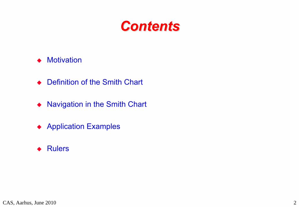
In the old days when no network analyzers were available, the In the old days when no network analyzers were available, the reflection coefficient was measured using a coaxial measurement reflection coefficient was measured using a coaxial measurement line with a slit in axial direction:line with a slit in axial direction:
RF measurements like this are now obsolete, but the Smith Chart,RF measurements like this are now obsolete, but the Smith Chart,
the VSWR and the reflection coefficient the VSWR and the reflection coefficient ΓΓ
are still very important and are still very important and used in the everyday life of the microwave engineer both for used in the everyday life of the microwave engineer both for simulations and measurementssimulations and measurements
CAS, Aarhus, June 2010 4
There was a little electric field probe There was a little electric field probe protruding into the field region of this protruding into the field region of this coaxial line near the outer conductor coaxial line near the outer conductor and the signal picked up was and the signal picked up was rectified in a microwave diode and rectified in a microwave diode and displayed on a micro volt meterdisplayed on a micro volt meter
Going along this RF measurement Going along this RF measurement line, one could find minima and line, one could find minima and maxima and determine their position, maxima and determine their position, spacing and the ratio of maximum to spacing and the ratio of maximum to minimum voltage reading. This is minimum voltage reading. This is the origin of the VSWR (voltage the origin of the VSWR (voltage standing wave ratio) which we will standing wave ratio) which we will discuss later again in more detail discuss later again in more detail
Movable electric field probe
DUT or terminating impedance
from generator
RF Basic Concepts, Caspers, McIntosh, Kroyer 5
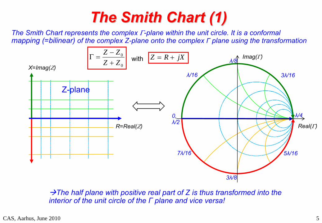
The Smith Chart (1)The Smith Chart (1)
Smith Chart
The Smith Chart represents the complex -plane within the unit circle. It is a conformal mapping (=bilinear)
of the complex Z-plane onto the complex Γ
plane using the transformation
0
0
ZZZZ
The half plane with positive real part of Z is thus transformed into the interior of the unit circle of the Γ
plane and vice versa!
R=Real()
X=Imag()
Real()
Imag()
CAS, Aarhus, June 2010
0, λ/2
λ/16
λ/8
3λ/16
λ/4
3λ/8
5λ/167λ/16
with jXRZ
Z-plane
RF Basic Concepts, Caspers, McIntosh, Kroyer 6
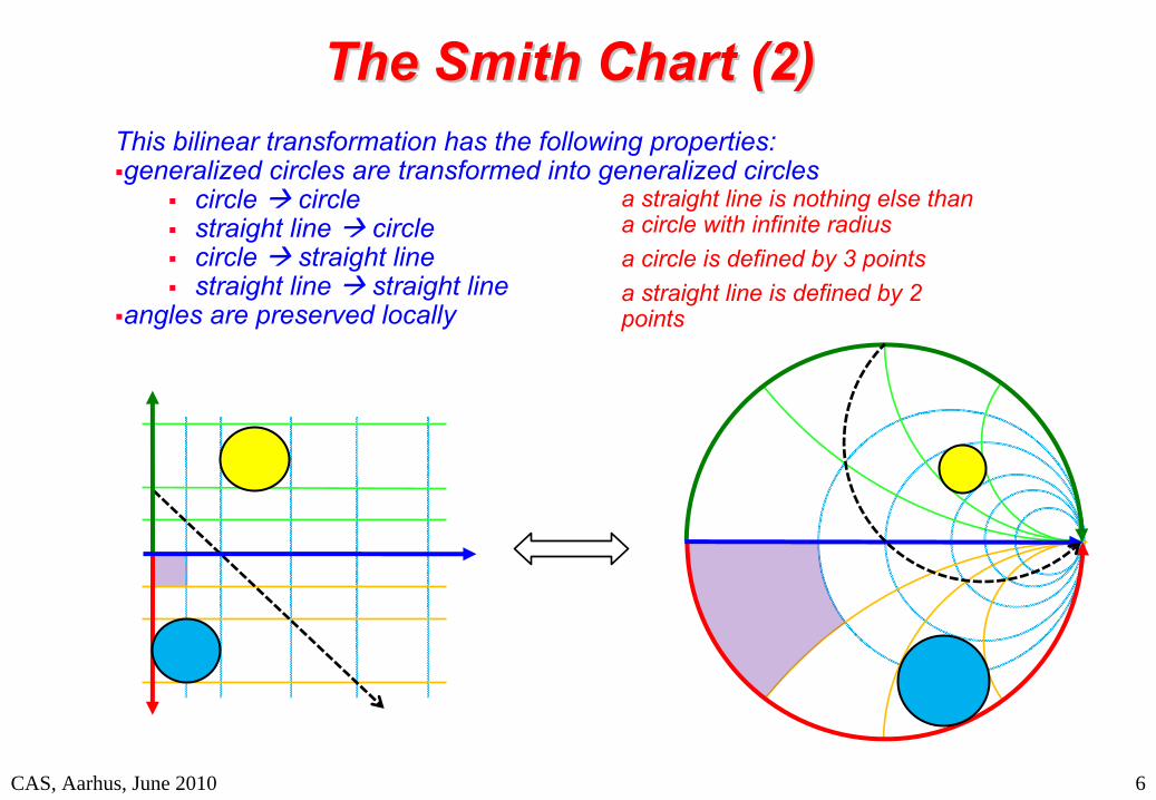
The Smith Chart (2)The Smith Chart (2)
Smith Chart
This bilinear transformation has the following properties:generalized circles are transformed into generalized circles
circle circle
straight line circle
circle straight line
straight line straight lineangles are preserved locally
a straight line is nothing else than a circle with infinite radiusa circle is defined by 3 pointsa straight line is defined by 2 points
CAS, Aarhus, June 2010
RF Basic Concepts, Caspers, McIntosh, Kroyer 7
The Smith Chart (3)The Smith Chart (3)
Smith Chart
Impedances Z are usually first normalized by
where Z0
is some reference impedance which is often the characteristic impedance of the connecting coaxial cables (e.g. 50 Ohm). The general form of the
transformation can then be written as
This mapping offers several practical advantages:
1.
The diagram includes all “passive”
impedances, i.e. those with positive real part, from zero to infinity in a handy format. Impedances with negative real part (“active device”, e.g. reflection amplifiers) would show up outside the (normal) Smith chart.2.
The mapping converts impedances (z) or admittances (y) into reflection factors and vice-
versa. This is particularly interesting for studies in the radiofrequency and microwave domain where electrical quantities are usually expressed in terms of “direct”
or “forward”
waves and “reflected”
or “backward”
waves. This replaces the notation in terms of currents and voltages used at lower frequencies. Also the reference plane can be moved
very easily using the Smith chart.
0ZZz
11
.11 zresp
zz
CAS, Aarhus, June 2010
RF Basic Concepts, Caspers, McIntosh, Kroyer 8
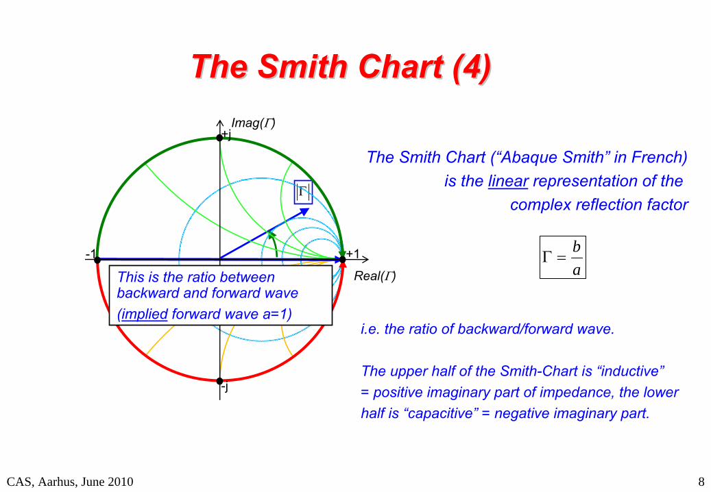
The Smith Chart (4)The Smith Chart (4)
Smith Chart
The Smith Chart (“Abaque Smith”
in French)is the linear
representation of the complex reflection factor
i.e. the ratio of backward/forward wave.
The upper half of the Smith-Chart is “inductive”= positive imaginary part of impedance, the lowerhalf is “capacitive”
= negative imaginary part.
ab
CAS, Aarhus, June 2010
Real()
Imag()
This is the ratio between backward and forward wave(implied
forward wave a=1)
+j
-j
-1 +1
RF Basic Concepts, Caspers, McIntosh, Kroyer 9
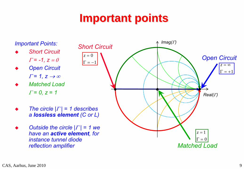
Important pointsImportant points
Short Circuit
Matched
Load
Open Circuit
Important Points:
Short Circuit = -1, z
Open Circuit = 1, z
Matched Load = 0, z = 1
The circle | | = 1 describes a lossless element (C or L)
Outside the circle | | = 1 we have an active element, for instance tunnel diode reflection amplifier
Smith Chart
1z1
0
z
01
z
CAS, Aarhus, June 2010
Real()
Imag()

RF Basic Concepts, Caspers, McIntosh, Kroyer 10
The Smith Chart (5)The Smith Chart (5)
Smith Chart
The Smith Chart can also represent the complex -plane within the unit circle using a conformal mapping
of the complex Y-plane onto itself using the transformation
0
0
0
0
0
0
11
11
ZZZZ
ZZ
ZZYYYY
G=Real(Y)
B=Imag(Y)
CAS, Aarhus, June 2010
Imag()
Real()
with jBGY
Y-plane
RF Basic Concepts, Caspers, McIntosh, KroyerCAS, Aarhus, June 2010 11
How does it look like:How does it look like:
Answer: VERY CONFUSING!

RF Basic Concepts, Caspers, McIntosh, Kroyer 12
The Smith Chart (6)The Smith Chart (6)
Smith Chart
Here the US notion is used, where power = |a|2.
European notation (often): power = |a|2/2
These conventions have no impact on S parameters, but is relevant for absolute power calculation which is rarely used in the Smith Chart
3.
The distance from the center of the diagram is directly proportional to the magnitude of the reflection factor. In particular, the perimeter
of the diagram represents full reflection, ||=1. Problems of matching are clearly visualize.
Power into the load = forward power –
reflected power
22
22
1
a
baP
“(mismatch)”
loss
available power from the source
0
25.0
5.0
75.0
1
CAS, Aarhus, June 2010
RF Basic Concepts, Caspers, McIntosh, Kroyer 13
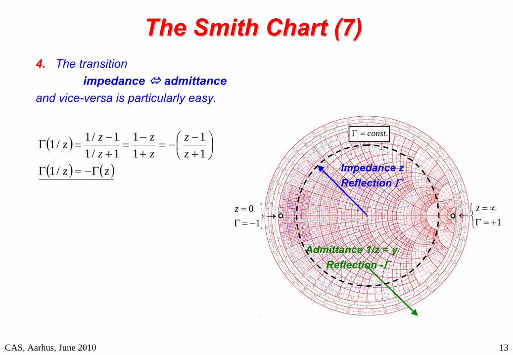
The Smith Chart (7)The Smith Chart (7)
Smith Chart
4.
The transitionimpedance admittance
and vice-versa is particularly easy.
zzzz
zz
zzz
/111
11
1/11/1/1
CAS, Aarhus, June 2010
Impedance zReflection
Admittance 1/z = yReflection -
.const
1
z
10z
RF Basic Concepts, Caspers, McIntosh, Kroyer 14
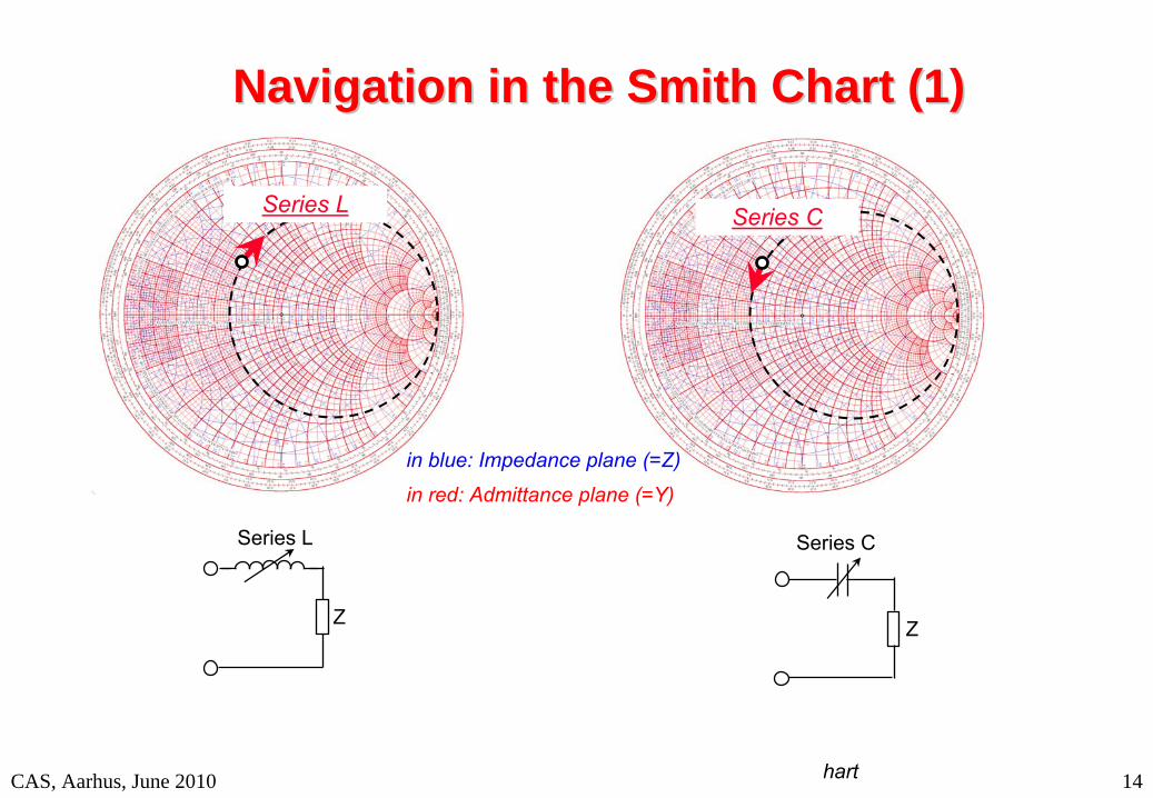
Navigation in the Smith Chart (1)Navigation in the Smith Chart (1)
Series L
Navigation in the Smith ChartCAS, Aarhus, June 2010
Series L
Series C
Series L
Z
Series C
Z
in blue: Impedance plane (=Z)
in red: Admittance plane (=Y)

RF Basic Concepts, Caspers, McIntosh, Kroyer 15
Navigation in the Smith Chart (2)Navigation in the Smith Chart (2)
Shunt L
Navigation in the Smith ChartCAS, Aarhus, June 2010
Series L
Shunt C
Shunt L
Z
Shunt C
Z
in blue: Admittance plane (=Y)
in red: Impedance plane (=Z)
RF Basic Concepts, Caspers, McIntosh, Kroyer 16
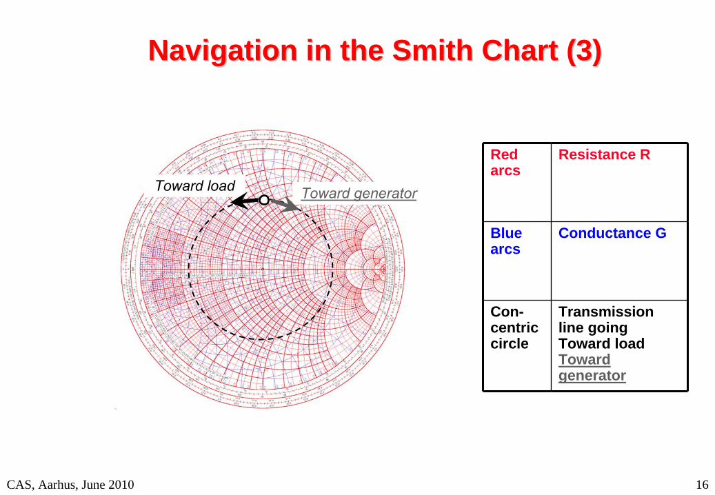
Navigation in the Smith Chart (3)Navigation in the Smith Chart (3)
Red arcs
Resistance R
Blue arcs
Conductance G
Con- centric circle
Transmission line going Toward load Toward generator
Toward generatorToward load
Navigation in the Smith ChartCAS, Aarhus, June 2010
RF Basic Concepts, Caspers, McIntosh, Kroyer 17
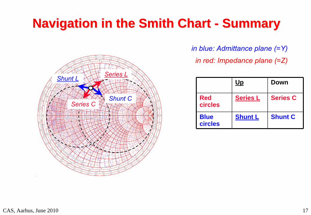
Navigation in the Smith Chart Navigation in the Smith Chart -- SummarySummary
Up Down
Red circles
Series L Series C
Blue circles
Shunt L Shunt C
Series L
Series C
Shunt L
Shunt C
Navigation in the Smith Chart
in blue: Admittance plane (=Y)
in red: Impedance plane (=Z)
CAS, Aarhus, June 2010
RF Basic Concepts, Caspers, McIntosh, Kroyer
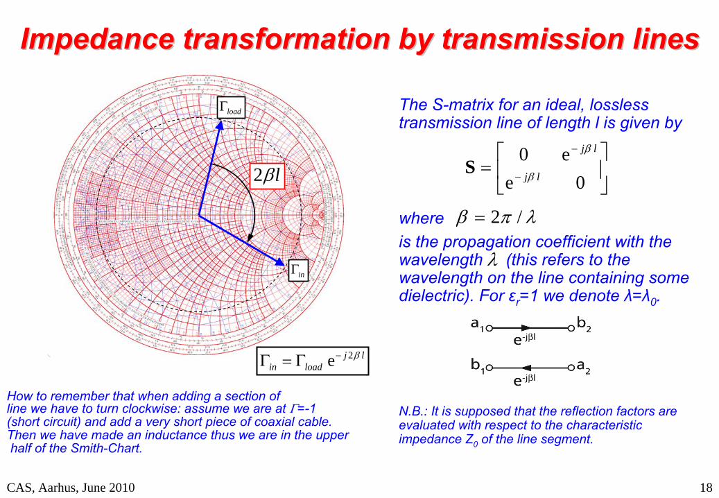
The S-matrix for an ideal, lossless transmission line of length l is given by
whereis the propagation coefficient with the wavelength (this refers to the wavelength on the line containing some dielectric). For εr
=1 we denote λ=λ0
.
N.B.: It is supposed that the reflection factors are evaluated with respect to the characteristic impedance Z0
of the line segment.
18
Impedance transformation by transmission linesImpedance transformation by transmission lines
Navigation in the Smith Chart
0ee0
lj
lj
S
/2
How to remember that when adding a section ofline we have to turn clockwise: assume we are at =-1(short circuit) and add a very short piece of coaxial cable. Then we have made an inductance thus we are in the upperhalf of the Smith-Chart.
in
ljloadin
2e
load
l2
CAS, Aarhus, June 2010
RF Basic Concepts, Caspers, McIntosh, Kroyer 19
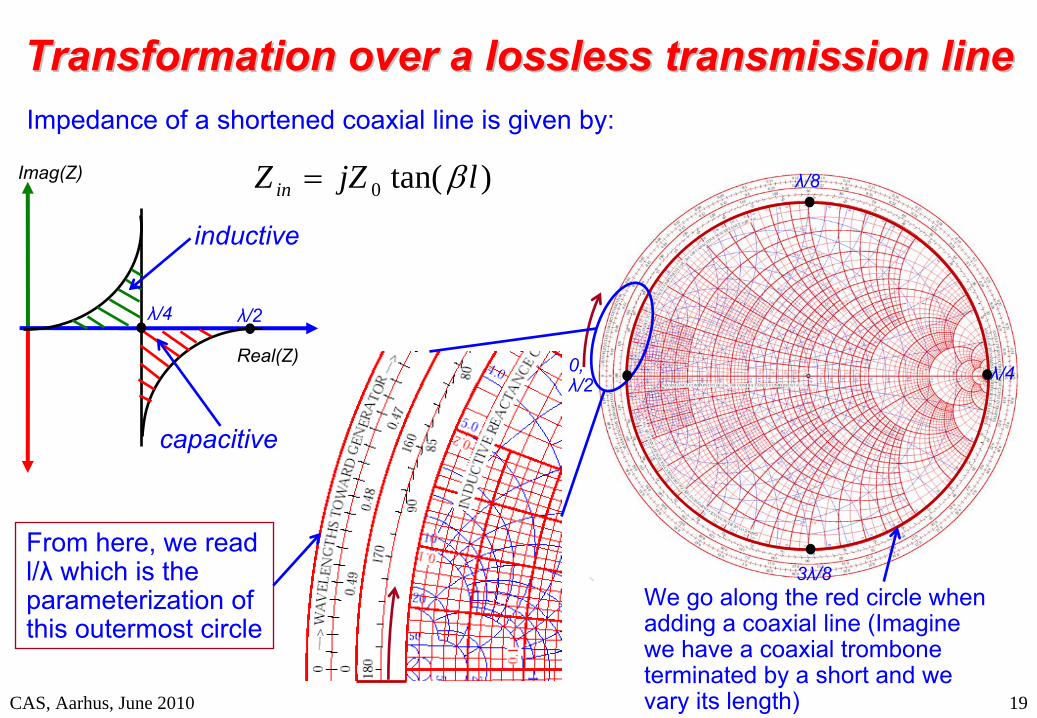
Transformation over a lossless transmission lineTransformation over a lossless transmission lineImpedance of a shortened coaxial line is given by:
)tan(0 ljZZ in
CAS, Aarhus, June 2010
From here, we read l/λ
which is the parameterization of this outermost circle
We go along the red circle when adding a coaxial line (Imagine we have a coaxial trombone terminated by a short and we vary its length)
Real(Z)
Imag(Z)
inductive
capacitive
λ/4 λ/2
0, λ/2
λ/8
λ/4
3λ/8
RF Basic Concepts, Caspers, McIntosh, Kroyer 20
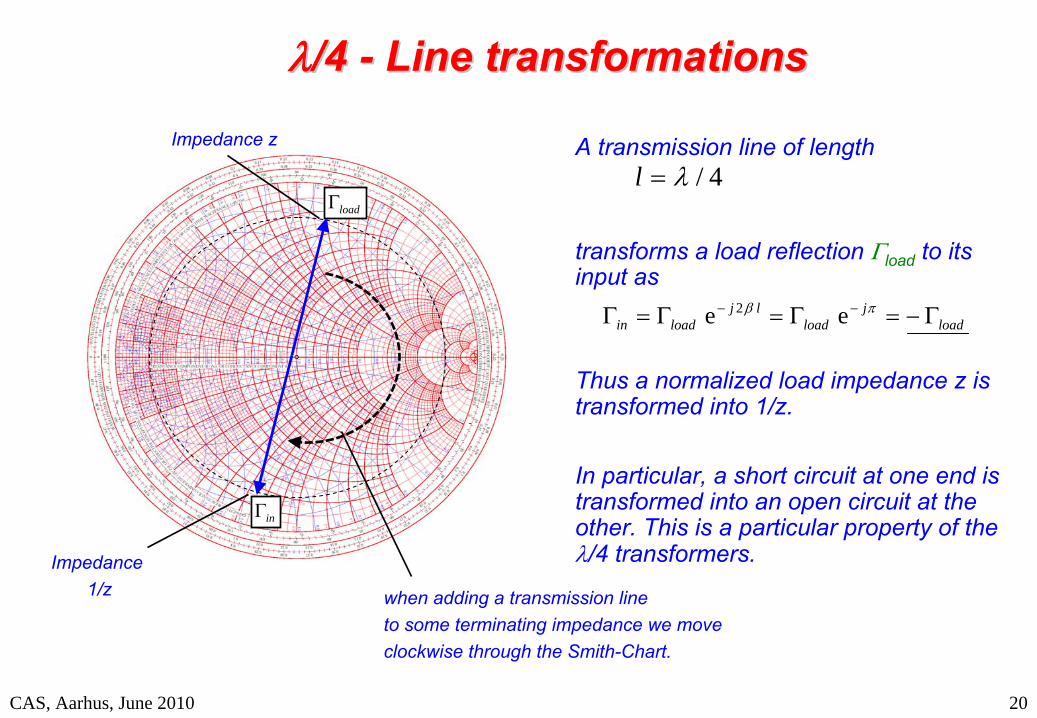
/4 /4 -- Line transformationsLine transformations
Navigation in the Smith Chart
A transmission line of length
transforms a load reflection load
to its input as
Thus a normalized load impedance z is transformed into 1/z.
In particular, a short circuit at one end is transformed into an open circuit at the other. This is a particular property of the /4 transformers.
4/l
loadj
loadlj
loadin ee 2
load
in
Impedance z
Impedance 1/z when adding a transmission line
to some terminating impedance we move clockwise through the Smith-Chart.
CAS, Aarhus, June 2010

RF Basic Concepts, Caspers, McIntosh, Kroyer
L
Lin S
SSS
22
211211 1
In general:
were in
is the reflection coefficient when looking through the 2-port and load
is the load reflection coefficient.
The outer circle and the real axis in the simplified Smith diagram below are mapped to other circles and lines, as can be seen on the right.
21
Looking through a 2Looking through a 2--port port
Line /16 (= π/8):
Attenuator 3dB:
0ee0
8j
8j
4je
Lin
in
L
1 2
022
220
2L
in
in
L
1 2
0
1
0 1
z = 0 z = z = 1 orZ = 50
Navigation in the Smith ChartCAS, Aarhus, June 2010
terminating impedance
Transformer with e-2βl
Increasing
terminating resistor
Variable load resistor (0<z<∞):
RF Basic Concepts, Caspers, McIntosh, Kroyer 22
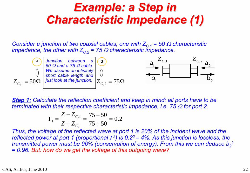
Example: a Step in Example: a Step in Characteristic Impedance (1) Characteristic Impedance (1)
Example
Consider a junction of two coaxial cables, one with ZC,1
= 50 characteristic impedance, the other with ZC,2
= 75 characteristic impedance.
11
ROLLET
LINVILL
KK
Junction between a 50
and a 75 cable. We assume an infinitely short cable length and just look at the junction.
1 2
501,CZ 752,CZ
1,CZ 2,CZ
Step 1:
Calculate the reflection coefficient and keep in mind: all ports have to be terminated with their respective characteristic impedance, i.e. 75
for port 2.
Thus, the voltage of the reflected wave at port 1 is 20% of the incident wave and the reflected power at port 1 (proportional 2) is 0.22 = 4%. As this junction is lossless, the transmitted power must be 96% (conservation of energy). From this we can deduce b2
2
= 0.96. But: how do we get the voltage of this outgoing wave?
2.050755075
1,
1,1
C
C
ZZZZ
CAS, Aarhus, June 2010
RF Basic Concepts, Caspers, McIntosh, Kroyer 23
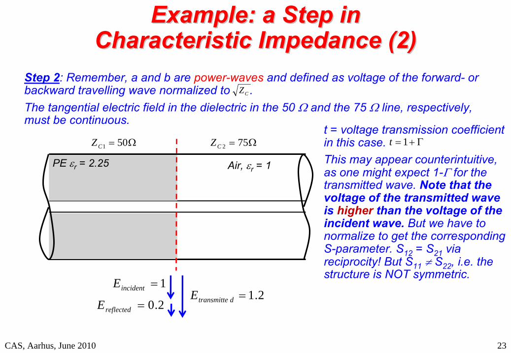
Example: a Step in Example: a Step in Characteristic Impedance (2) Characteristic Impedance (2)
Example
Step 2: Remember, a and b are power-waves
and defined as voltage of the forward-
or backward travelling wave normalized to .The tangential electric field in the dielectric in the 50
and the 75
line, respectively, must be continuous.
501CZ
CZ
PE r
= 2.25 Air, r
= 1
752CZ
1incidentE
2.0reflectedE2.1dtransmitteE
t = voltage transmission coefficient in this case.This may appear counterintuitive, as one might expect 1- for the transmitted wave. Note that the voltage of the transmitted wave is higher
than the voltage of the incident wave.
But we have to normalize to get the corresponding S-parameter. S12
= S21
via reciprocity! But S11
S22
, i.e. the structure is NOT symmetric.
1t
CAS, Aarhus, June 2010
RF Basic Concepts, Caspers, McIntosh, Kroyer 24
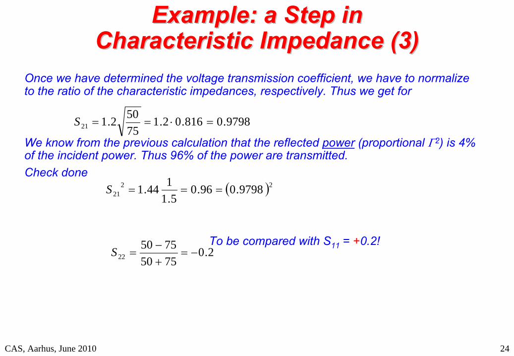
Example: a Step in Example: a Step in Characteristic Impedance (3) Characteristic Impedance (3)
Example
Once we have determined the voltage transmission coefficient, we
have to normalize to the ratio of the characteristic impedances, respectively. Thus we get for
We know from the previous calculation that the reflected power
(proportional 2) is 4% of the incident power. Thus 96% of the power are transmitted. Check done
To be compared with S11
= +0.2!
9798.0816.02.175502.121 S
2221 9798.096.0
5.1144.1 S
2.075507550
22
S
CAS, Aarhus, June 2010

RF Basic Concepts, Caspers, McIntosh, Kroyer 25Example
-b b = +0.2
incident wave a = 1
Vt
= a+b = 1.2
It Z = a-b
Example: a Step in Example: a Step in Characteristic Impedance (4) Characteristic Impedance (4)
Visualization in the Smith chart
As shown in the previous slides the transmitted voltage ist = 1 + Vt
= a + b
and subsequently the current isIt
Z = a -
b. Remember: the reflection coefficient is defined with respect to voltages. For currents the sign inverts. Thus a positive reflection coefficient in the normal (=voltage) definition leads to a subtraction of currents or is negative with respect to current.
Note: here Zload
is real
CAS, Aarhus, June 2010
RF Basic Concepts, Caspers, McIntosh, Kroyer 26
-b
B ~ Γ
a = 1
V1= a+b
I1 Z = a-b
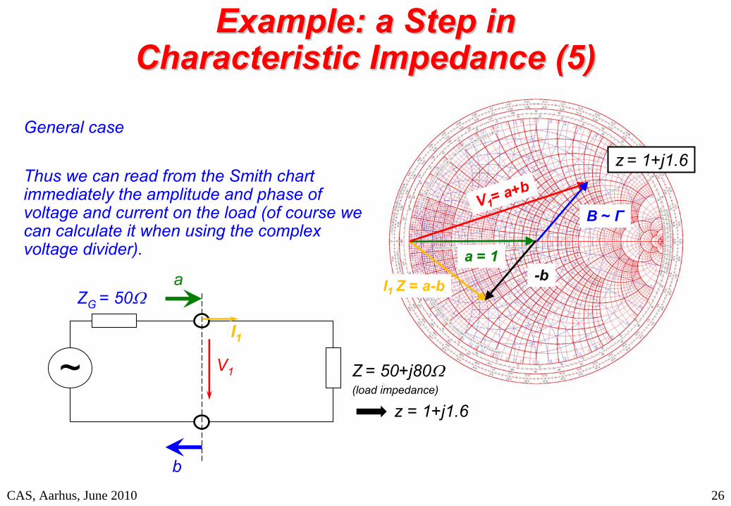
Example: a Step in Example: a Step in Characteristic Impedance (5) Characteristic Impedance (5)
General case
Thus we can read from the Smith chart immediately the amplitude and phase of voltage and current on the load (of course we can calculate it when using the complex voltage divider).
Z
= 50+j80(load impedance)
z = 1+j1.6
~
ZG = 50
V1
a
b
I1
z
= 1+j1.6
ExampleCAS, Aarhus, June 2010

RF Basic Concepts, Caspers, McIntosh, Kroyer 27
What about all these rulers What about all these rulers below the Smith chart (1)below the Smith chart (1)
How to use these rulers:You take the modulus of the reflection coefficient of an impedance to be examined by some means, either with a conventional ruler or better take it into the compass. Then refer to the coordinate denoted to CENTER and go to the left or for the other part of the rulers (not shown here in the magnification) to the right except for the lowest line which is marked ORIGIN at the left.
ExampleCAS, Aarhus, June 2010

RF Basic Concepts, Caspers, McIntosh, Kroyer 28
What about all these rulers What about all these rulers below the Smith chart (2)below the Smith chart (2)
First ruler / left / upper part, marked SWR. This means VSWR, i.e. Voltage Standing Wave Ratio, the range of value is between one and infinity. One is for the matched case (center of the Smith chart), infinity is for total reflection (boundary of the SC). The upper part is in linear scale, the lower part of this ruler is in dB, noted as dBS (dB referred to Standing Wave Ratio). Example: SWR = 10 corresponds to 20 dBS, SWR = 100 corresponds to 40 dBS [voltage ratios, not power ratios].
ExampleCAS, Aarhus, June 2010
RF Basic Concepts, Caspers, McIntosh, Kroyer 29
What about all these rulers What about all these rulers below the Smith chart (3)below the Smith chart (3)
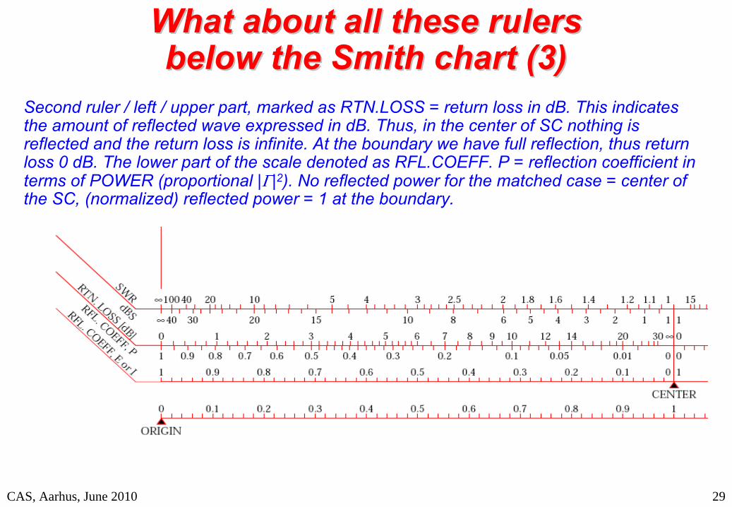
Second ruler / left / upper part, marked as RTN.LOSS = return loss in dB. This indicates the amount of reflected wave expressed in dB. Thus, in the center of SC nothing is reflected and the return loss is infinite. At the boundary we have full reflection, thus return loss 0 dB. The lower part of the scale denoted as RFL.COEFF. P =
reflection coefficient in terms of POWER (proportional ||2). No reflected power for the matched case = center of the SC, (normalized) reflected power = 1 at the boundary.
ExampleCAS, Aarhus, June 2010
RF Basic Concepts, Caspers, McIntosh, Kroyer 30
What about all these rulers What about all these rulers below the Smith chart (4)below the Smith chart (4)
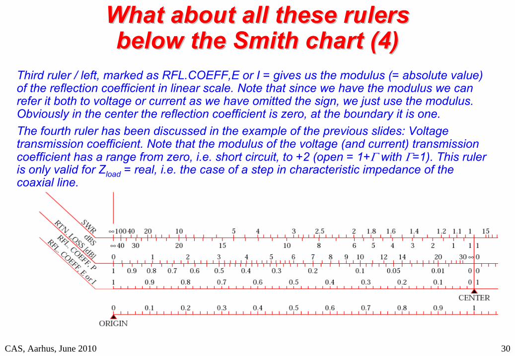
Third ruler / left, marked as RFL.COEFF,E or I = gives us the modulus (= absolute value) of the reflection coefficient in linear scale. Note that since we have the modulus we can refer it both to voltage or current as we have omitted the sign,
we just use the modulus. Obviously in the center the reflection coefficient is zero, at the boundary it is one. The fourth ruler has been discussed in the example of the previous slides: Voltage transmission coefficient. Note that the modulus of the voltage (and current) transmission coefficient has a range from zero, i.e. short circuit, to +2 (open = 1+ with =1).
This ruler is only valid for Zload
= real, i.e. the case of a step in characteristic impedance of the coaxial line.
ExampleCAS, Aarhus, June 2010
RF Basic Concepts, Caspers, McIntosh, Kroyer 31
What about all these rulers What about all these rulers below the Smith chart (5)below the Smith chart (5)
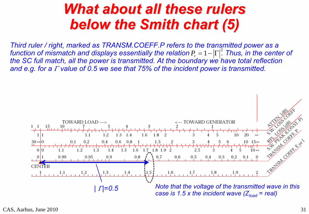
Third ruler / right, marked as TRANSM.COEFF.P refers to the transmitted power as a function of mismatch and displays essentially the relation . Thus, in the center of the SC full match, all the power is transmitted. At the boundary
we have total reflection and e.g. for a value of 0.5 we see that 75% of the incident power is transmitted.
Example
21 tP
|
|=0.5 Note that the voltage of the transmitted wave in this case is 1.5 x the incident wave (Zload
= real)
CAS, Aarhus, June 2010
RF Basic Concepts, Caspers, McIntosh, Kroyer 32
What about all these rulers What about all these rulers below the Smith chart (6)below the Smith chart (6)
Example
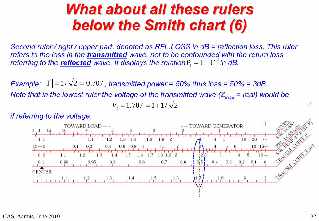
Second ruler / right / upper part, denoted as RFL.LOSS in dB = reflection loss. This ruler refers to the loss in the transmitted
wave, not to be confounded with the return loss referring to the reflected
wave. It displays the relation in dB.
Example: , transmitted power = 50%
thus loss = 50% = 3dB. Note that in the lowest ruler the voltage of the transmitted wave (Zload
= real)
would be
if referring to the voltage.
21 tP
707.02/1
2/11707.1 tV
CAS, Aarhus, June 2010

RF Basic Concepts, Caspers, McIntosh, Kroyer 33
What about all these rulers What about all these rulers below the Smith chart (7)below the Smith chart (7)
Example
Another Example: 3dB attenuator gives forth and back 6dB which is half the voltage.
First ruler / right / upper part, denoted as ATTEN. in dB assumes that we are measuring an attenuator (that may be a lossy line) which itself is terminated
by an open or short circuit (full reflection). Thus the wave is travelling twice through the
attenuator (forward and backward). The value of this attenuator can be between zero and some very high number corresponding to the matched case. The lower scale of ruler #1 displays the same situation just in terms of VSWR.Example: a 10dB attenuator attenuates the reflected wave by 20dB
going forth and back and we get a reflection coefficient of =0.1 (= 10% in voltage).
CAS, Aarhus, June 2010
RF Basic Concepts, Caspers, McIntosh, Kroyer
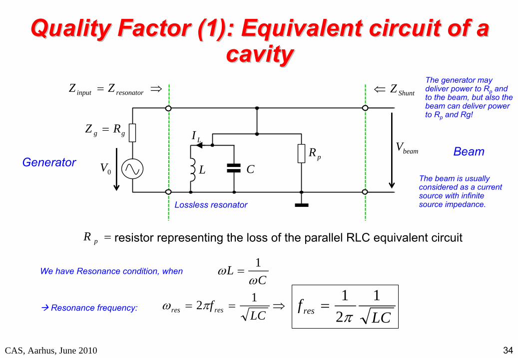
Lossless resonator
LI
L CpR beamV
0V
gg RZ
34
LC
fresres12
Quality Factor (1): Equivalent circuit of a Quality Factor (1): Equivalent circuit of a cavity cavity
Generator
We have Resonance condition, when
LCfres
121
Equivalent circuit
Beam
resonatorinput ZZ
pR
CL
1
ShuntZ
Resonance frequency:
The beam is usually considered as a current source with infinite source impedance.
The generator may deliver power to Rp
and to the beam, but also the beam can deliver power to Rp
and Rg!
CAS, Aarhus, June 2010
resistor representing the loss of the parallel RLC equivalent circuit

RF Basic Concepts, Caspers, McIntosh, KroyerCAS, Aarhus, June 2010 35
The quality (Q) factor of a resonant circuit is defined as the ratio of the stored energy W over the energy dissipated P
in one cycle.
Q0
: Unloaded Q factor of the unperturbed system, e.g. the “stand alone”cavity
QL
: Loaded Q factor:
generator and measurement circuits connected
Qext
: External Q factor describes the degradation of Q0
due to generator and diagnostic impedances
These Q factors are related by
The Q factor of a resonance can be calculated from the center frequency f0
and the 3 dB bandwidth f
as
PWQ
extL QQQ111
0
ffQ
0
The Quality Factor (2)The Quality Factor (2)
RF Basic Concepts, Caspers, McIntosh, Kroyer 36
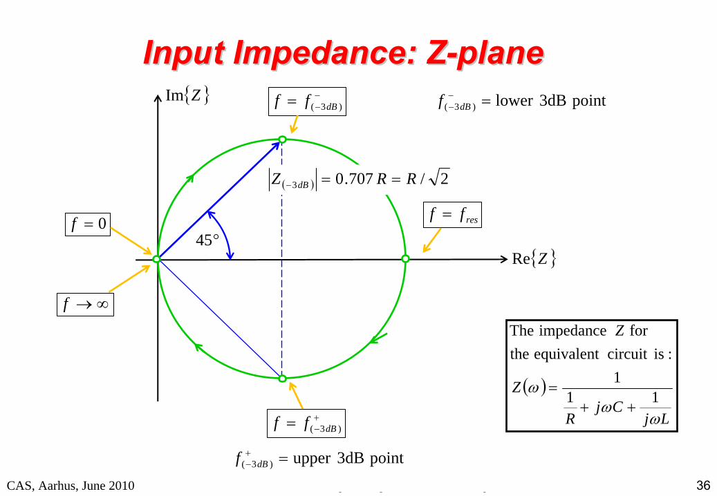
Input Impedance: ZInput Impedance: Z--planeplane
LjCj
R
Z
Z
111
:iscircuit equivalent thefor impedance The
0f
f
ZRe
ZIm
45
)3( dBff
)3( dBff
resff
point 3dBlower )3( dBf
point 3dBupper )3( dBf
2/707.03 RRZ dB
Equivalent circuitCAS, Aarhus, June 2010
RF Basic Concepts, Caspers, McIntosh, Kroyer 37
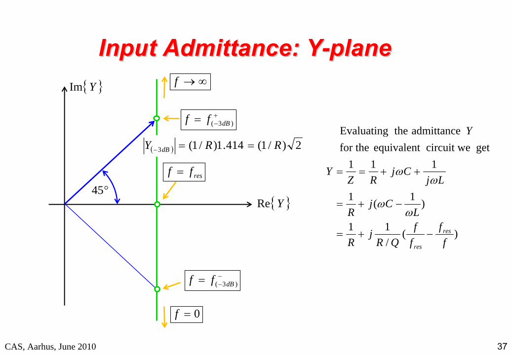
Input Admittance: YInput Admittance: Y--planeplane
)(/11
)1(1
111get circuit we equivalent for the
admittancetheEvaluating
ff
ff
QRj
R
LCj
R
LjCj
RZY
Y
res
res
0f
f
YRe
YIm
45resff
)3( dBff
)3( dBff
2)/1(414.1)/1(3 RRY dB
Equivalent circuitCAS, Aarhus, June 2010

RF Basic Concepts, Caspers, McIntosh, KroyerCAS, Aarhus, June 2010 38
The typical locus of a resonant circuit in the Smith chart is illustrated as the dashed red circle (shown in the “detuned short”
position)
From the different marked frequency points the 3 dB bandwidth and thus the quality factors Q0 (f5
,f6
), QL
(f1
,f2
) and Qext
(f3
,f4
) can be determined
The larger the circle, the stronger the coupling
In practise, the circle may be rotated around the origin due to transmission lines between the resonant circuit and the measurement device
QQ--Factor Measurement in the Smith Chart Factor Measurement in the Smith Chart Locus of Re(Z)=Im(Z)
RF Basic Concepts, Caspers, McIntosh, Kroyer
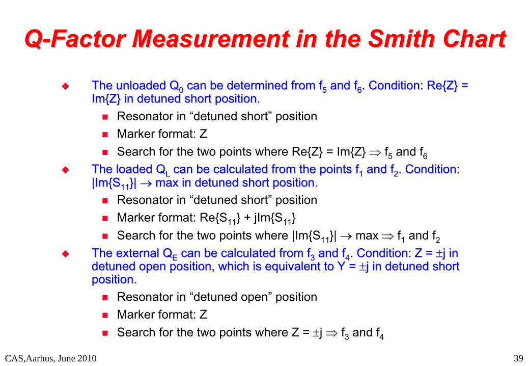
The unloaded QThe unloaded Q00
can be determined from fcan be determined from f55
and fand f66
. Condition: . Condition: Re{ZRe{Z} = } = Im{ZIm{Z} in detuned short position. } in detuned short position.
Resonator in “detuned short”
position
Marker format: Z
Search for the two points where Re{Z} = Im{Z} f5
and f6
The loaded QThe loaded QLL
can be calculated from the points fcan be calculated from the points f11
and fand f22
. Condition: . Condition: |Im{S|Im{S1111
}| }|
max in detuned short position. max in detuned short position.
Resonator in “detuned short”
position
Marker format: Re{S11
} + jIm{S11
}
Search for the two points where |Im{S11
}| max f1
and f2
The external QThe external QEE
can be calculated from fcan be calculated from f33
and fand f44
. Condition: Z = . Condition: Z = j in j in detuned open position, which is equivalent to Y = detuned open position, which is equivalent to Y = j in detuned short j in detuned short position.position.
Resonator in “detuned open”
position
Marker format: Z
Search for the two points where Z = j f3
and f4
CAS,Aarhus, June 2010 39
QQ--Factor Measurement in the Smith Chart Factor Measurement in the Smith Chart
RF Basic Concepts, Caspers, McIntosh, Kroyer
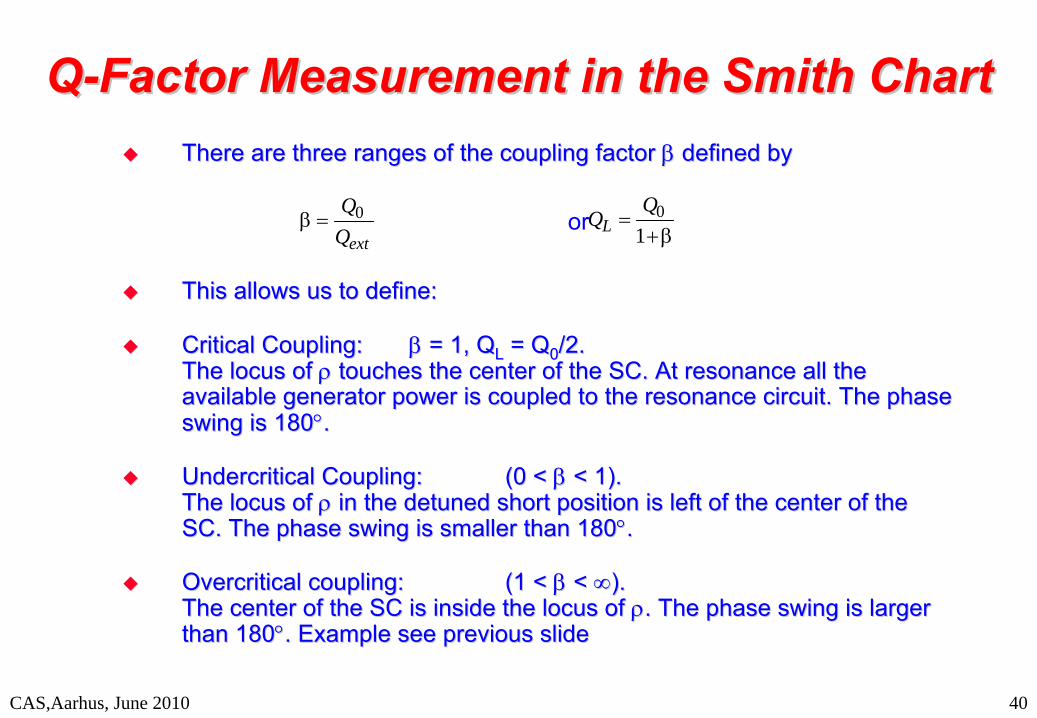
There are three ranges of the coupling factor There are three ranges of the coupling factor
defined bydefined by
or
This allows us to define:This allows us to define:
Critical Coupling: Critical Coupling:
= 1, Q= 1, QLL
= Q= Q00
/2. /2. The locus of The locus of
touches the center of the SC. At resonance all the touches the center of the SC. At resonance all the available generator power is coupled to the resonance circuit. Tavailable generator power is coupled to the resonance circuit. The phase he phase swing is 180swing is 180..
UndercriticalUndercritical
Coupling: Coupling: (0 < (0 <
< 1). < 1). The locus of The locus of
in the detuned short position is left of the center of the in the detuned short position is left of the center of the SC. The phase swing is smaller than 180SC. The phase swing is smaller than 180..
Overcritical coupling: Overcritical coupling: (1 < (1 <
< < ). ). The center of the SC is inside the locus of The center of the SC is inside the locus of . The phase swing is larger . The phase swing is larger than 180than 180. Example see previous slide. Example see previous slide
CAS,Aarhus, June 2010 40
0
ext
01LQ
Q
QQ--Factor Measurement in the Smith Chart Factor Measurement in the Smith Chart


![[DE] Dokumentationen als nutzbares Wissen bereitstellen am Beispiel der PROJECT CONSULT Newsletter | Paul Caspers | Update Information Management 2016](https://img.dokumen.tips/doc/110x75/58ed70f91a28abe1448b45d9/de-dokumentationen-als-nutzbares-wissen-bereitstellen-am-beispiel-der-project.jpg)