HAL Id: hal-01281219https://hal.archives-ouvertes.fr/hal-01281219

Preprint submitted on 1 Mar 2016

HAL is a multi-disciplinary open accessarchive for the deposit and dissemination of sci-entific research documents, whether they are pub-lished or not. The documents may come fromteaching and research institutions in France orabroad, or from public or private research centers.

L’archive ouverte pluridisciplinaire HAL, estdestinée au dépôt et à la diffusion de documentsscientifiques de niveau recherche, publiés ou non,émanant des établissements d’enseignement et derecherche français ou étrangers, des laboratoirespublics ou privés.

REWRITING IN HIGHER DIMENSIONAL LINEARCATEGORIES AND APPLICATION TO THEAFFINE ORIENTED BRAUER CATEGORY

Clément Alleaume

To cite this version:Clément Alleaume. REWRITING IN HIGHER DIMENSIONAL LINEAR CATEGORIES AND AP-PLICATION TO THE AFFINE ORIENTED BRAUER CATEGORY. 2016. �hal-01281219�

REWRITING IN HIGHER DIMENSIONAL LINEAR CATEGORIES AND

APPLICATION TO THE AFFINE ORIENTED BRAUER CATEGORY

Clément Alleaume

Univ Lyon, Université Claude Bernard Lyon 1, CNRS UMR 5208,

Institut Camille Jordan, 43 blvd. du 11 novembre 1918, F-69622 Villeurbanne cedex, France

clement.alleaume@univ-st-etienne.fr

Abstract – In this paper, we introduce a rewriting theory of linear monoidal categories. Those cat-

egories are a particular case of what we will define as linear (n, p)-categories. We will also define

linear (n, p)-polygraphs, a linear adapation of n-polygraphs, to present linear (n− 1, p)-categories.

We focus then on linear (3, 2)-polygraphs to give presentations of linear monoidal categories. We

finally give an application of this theory in linear (3, 2)-polygraphs to prove a basis theorem on the

category AOB with a new method using a rewriting property defined by van Ostroom: decreasing-

ness.

1. INTRODUCTION

Affine walled Brauer algebras were introduced by Rui and Su [RS13] in the study of super Schur-Weyl

duality. A result of [RS13] is the Schur-Weyl duality between general Lie superalgebras and affine walled

Brauer algebras. A linear monoidal category, the affine oriented Brauer category AOB was introduced

in [BCNR14] to encode each walled Brauer algebra as one of its morphism spaces. This category is used

to prove basis theorems for the affine walled Brauer algebras given in [RS13], which gives an explicit

basis for each affine walled Brauer algebra. The proof of this theorem uses an intermediate result on

cyclotomic quotients of AOB. For each of those quotients, a basis is given. With these multiple bases,

each morphism space of AOB is given a generating family which is proved to be linearly independent.

Our aim is to give a constructive proof of the mentioned basis result. For this, we study AOB

in this article by rewriting methods. Rewriting is a model of computation presenting relations between

expressions as oriented computation steps. There are multiple examples of rewriting systems. An abstract

rewriting system [Hue80] is the data of a set S and a relation → on S called the rewrite relation. A

rewriting sequence from a to b is a finite sequence (u0, u1, · · ·un−1, un) of elements of S such that:

a = u0,

b = un,

and for any 0 6 k < n, we have uk → uk+1. A word rewriting system is the data of an alphabet A

and a relation ⇒ on the free monoid A∗ over A. We say that there is a rewriting step from a word u to a

word v if there are words a, b, u ′ and v ′ such that:

u = au ′b,

v = av ′b,

u ′ ⇒ v ′.

A higher dimensional generalization of such rewriting systems has been introduced by Burroni [Bur93]

under the name of polygraph. An (n+1)-polygraph is a rewriting system on the n-cells of an n-category.

To study AOB from a rewriting point of view, we will need to introduce the rewriting systems

presenting monoidal linear categories. The objects giving such rewriting systems will be called lin-

ear (n, p)-polygraphs which are linear adaptations of n-polygraphs. Linear monoidal categories are a

special case of what we will call linear (n, p)-categories. In this language, linear monoidal categories

are linear (2, 2)-categories with only one 0-cell. They are presented by linear (3, 2)-polygraphs. Once

those objects are defined, we will introduce the rewriting theory of linear (3, 2)-polygraphs. Once we

have this theory, we will use it to construct bases for the morphism spaces of AOB.

Rewriting can offer constructive proofs by giving presentations of objects with certain properties. For

example, two properties studied in rewriting systems are termination and confluence. A rewriting system

1

is terminating if it has no infinite rewriting sequence, in which case all computations end. A rewriting

system is confluent if any pair of rewriting sequences with the same source can be completed into a pair

of rewriting sequences with the same target, in which case all computations lead to the same result. A

rewriting system is said to be convergent if it is terminating and confluent.In the case of word rewriting,

the property of convergence, the conjunction of termination and confluence, gives a way to decide the

word problem, that is, deciding if two words in A∗ are equal in the quotient of A∗ by the relation ⇒.

What we will do in the case of AOB is giving a confluent presentation AOB of this linear (2, 2)-

category with some others properties. Those properties will prove the bases given in [BCNR14] are in-

deed bases. The linear (3, 2)-polygraph AOB will not be terminating, which will prevent us to prove AOB

is confluent by the use of Newman’s lemma, a criterion needing termination to prove confluence from a

weaker property called local confluence [Hue80]. To prove AOB is confluent, we will use a more gen-

eral property called decreasingness introduced in [vO94]. We will prove AOB is decreasing and use the

theorem from [vO94] stating decreasingness implies confluence.

In the first section, we recall first the notions of higher dimensional category theory. Then, we

define linear (n, p)-categories, which will be our higher dimensional categories with linear structure.

After defining them, we recall in the second section the categorical construction of the category of n-

polygraphs given in [Mét08]. We define next the categorical construction of the category of linear (n, p)-

polygraphs. We give their main rewriting properties, such than 4.2.15 in the case (n, p) = (3, 2) in

which AOB falls.

In the third section we will study the decreasingness property defined in the case of abstract rewriting

systems by van Ostroom [vO94]. Then, in the last section, we recall from [BCNR14] the definition of

the linear (2, 2)-category AOB. This will lead us to give two linear (3, 2)-polygraphs presenting AOB.

Those linear (3, 2)-polygraphs will be called AOB and AOB. The first one is a translation of the definition

of AOB.

The main result of this article, Theorem 5.2.9 states AOB is confluent. It will be proved with the

properties of confluence of critical branchings and decreasingness. This theorem gives us the main result

of [BCNR14] as an entirely constructive consequence given as corollary 5.2.10.

ACKNOWLEDGMENTS

The author would like to thank Labex Milyon (ANR-10-LABX-0070). This work has been supported by

the project Cathre, ANR-13BS02-0005-02.

2. LINEAR (n, p)-CATEGORIES

This section and section 3 will recall the basic notions of n-category and n-polygraphs. The rewriting

techniques used in this paper will be presented in the last two sections.

2.1. Preliminaries

We fix n an integer. We denote by Set the category of sets.

2.1.1. Definition. An n-graph in a category C is a diagram in C:

G0

s0

t0

G1

s1

t1

· · ·

sn−2

tn−2

Gn−1

sn−1

tn−1

Gn

such that for any 1 6 k 6 n−1, we have sk−1 ◦sk = sk−1 ◦tk and tk−1 ◦sk = tk−1 ◦tk. Those relations

are called the globular relations. We just call an n-graph in Set an n-graph.

2

The elements of Gk are called k-cells. The maps sk and tk are respectively called k-source and k-

target maps. For any l-cell u of G with l > k+ 1, we respectively denote by sk(u) and tk(u) the k-cells

(sk ◦ · · · ◦ sl−1)(u) and (tk ◦ · · · ◦ tl−1)(u).

A morphism of n-graphs F from G to G ′ is a collection (Fk : Gk → G ′k) of maps such that, for

every 0 < k 6 n, the following diagrams commute:

Gk−1

sk−1

Gk

Fk−1 Fk

G ′k−1 s ′k−1

G ′k

Gk−1

tk−1

Gk

Fk−1 Fk

G ′k−1 t ′k−1

G ′k

We call Grphn the category of n-graphs.

In particular, Grph0 is the category Set and Grph1 is the category of directed graphs.

We can define n-categories by enrichment. A 0-category is a set. For n > 1, an n-category is a 1-

category enriched in (n−1)-categories. We denote by Catn the category of n-categories and n-functors.

This category has a terminal object In with only one k-cell for 0 6 k 6 n.

In an n-category, for any 0 6 k < n, we denote the k-composition by ⋆k. For all 0 6 i < j 6 n− 1

the following equality, called exchange relation, holds:

(u ⋆i v) ⋆j (u′⋆i v

′) = (u ⋆j u′) ⋆i (v ⋆j v

′). (1)

By forgetting its units and compositions, an n-category is in particular an n-graph. We now denote

by Un the forgetful functor from Catn to Grphn.

2.2. Linear (n, p)-categories

In this section, we fix n an integer. We will define linear (n, p)-categories by induction on p 6 n. We

will denote by Vect the category of vector spaces over a fixed field.

2.2.1. Definition. An internal n-category in Vect is the data of:

− an n-graph in Vect:

V0

s0

t0

V1

s1

t1

· · ·

sn−2

tn−2

Vn−1

sn−1

tn−1

Vn

− for each 0 6 k < l 6 n, a linear unit map v 7→ 1v from Vk to Vk+1. Linearity of the unit maps

gives us the following relation:

1λu+µv = λ1u + µ1v (2)

for any scalars λ and µ and any k-cells u and v such that p 6 k < n,

− for each 0 6 k < l 6 n, a linear composition map ⋆k from Vl ×VkVl to Vk. Linearity of the unit

maps gives us the following properties:

(f + g) ⋆k (f′ + g ′) = f ⋆k f

′ + g ⋆k g′, (3)

λf ⋆k λf′ = λ(f ⋆k f

′). (4)

for any scalar λ and any pairs (f, f ′) and (g, g ′) of k-composable l-cells such that p 6 k < l 6 n

verifying the axioms of n-categories.

3

Internal n-categories in Vect are also called (n + 1)-vector spaces [BC04], see also [KMP11].

2.2.2. Definition. A linear (n, 0)-category is an internal n-category in Vect. Let us assume linear (n, p)-

categories are defined for p > 0. A linear (n + 1, p+ 1)-category is the data of a set C0 and:

− for each a and b in C0, a linear (n, p)-category C(a, b),

− for each a in C0, an identity morphism ia from the terminal n-category In to C(a, a),

− for each a, b and c in C0, a bilinear composition morphism ⋆a,b,c from C(a, b)×C(b, c) to C(a, c).

such that:

− ⋆a,c,d ◦ (⋆a,b,c × idC(c,d)) = ⋆

a,b,d ◦ (idC(a,b) × ⋆b,c,d),

− ⋆a,a,b ◦(ia× idC(a,b))◦ isl = idC(a,b) = ⋆

a,b,b ◦(idC(a,b)× iq)◦ isr where isl and isr respectively

denote the canonic isomorphisms from C(a, b) to In × C(a, b) and to C(a, b)× In.

2.2.3. Remark. In particular, a linear (n, p)-category is an n-category.

A morphism of linear (n, p)-categories from C to C ′ is an n-functor:

C0

s0

t0

C1

s1

t1

· · ·

sn−2

tn−2

Cn−1

sn−1

tn−1

Cn

F0 F1 Fn−1 Fn

C ′0

s ′0

t ′0

C ′1

s ′1

t ′1

· · ·

s ′n−2

t ′n−2

C ′n−1

s ′n−1

t ′n−1

C ′n

such that for any p 6 k 6 n, the map Fk is linear. We denote by LinCatn,p the category of linear (n, p)-

categories. We denote by Un,p the forgetful functor from LinCatn,p to Grphn.

2.2.4. Example. A linear (1, 1)-category is just a linear category or a category enriched in vector

spaces as introduced by Mitchell [Mit72].

2.2.5. Remark. Let C be a linear (n, p)-category with 0 6 p < n. The underlying (n − 1)-category

to C is a linear (n − 1, p)-category. Indeed, there is an internal (n + p − 1)-graph in the category of

vector spaces given by:

Cp

sp

tp

Cp+1

sp+1

tp+1

· · ·

sn−3

tn−3

Cn−2

sn−2

tn−2

Cn−1

which can be completed into an (n − 1)-category:

C0

s0

t0

C1

s1

t1

· · ·

sp−2

tp−2

Cp−1

sp−1

tp−1

Cp

sp

tp

Cp+1

sp+1

tp+1

· · ·

sn−3

tn−3

Cn−2

sn−2

tn−2

Cn−1

The source maps, target maps and composition maps of this (n − 1)-category meet all the requirements

of a linear (n− 1, p)-category.

4

3. POLYGRAPHS

3.1. n-Polygraphs

The notion of polygraph was introduced by Burroni [Bur93]. It was introduced independently by Street

under the name of computad [Str87] as system of generators and relations for higher dimensional cate-

gories. Let us recall the constructions of the categories of n-categories with a globular extension and n-

polygraphs from [Mét08].

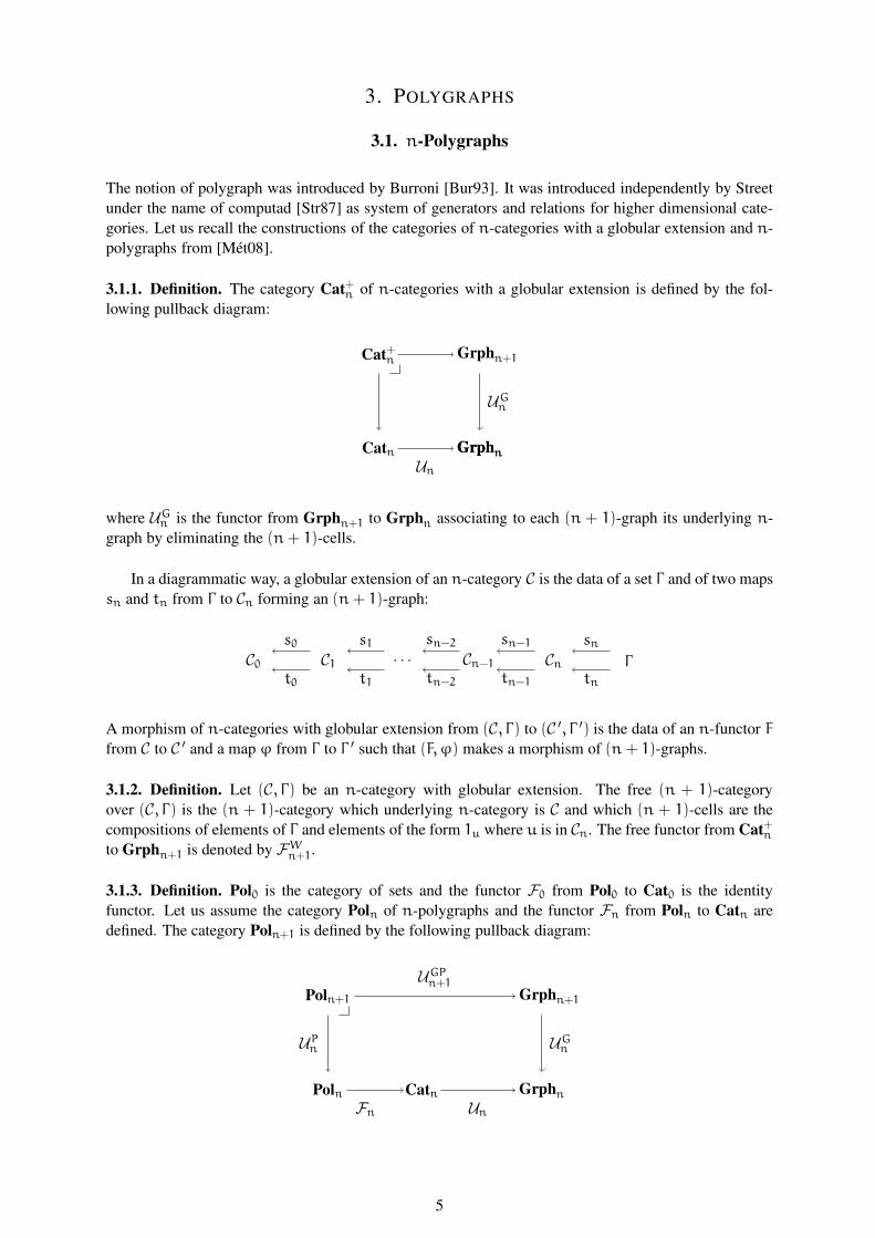
3.1.1. Definition. The category Cat+n of n-categories with a globular extension is defined by the fol-

lowing pullback diagram:

Cat+n Grphn+1

GrphnCatn Grphn

Un

UGn

where UGn is the functor from Grphn+1 to Grphn associating to each (n + 1)-graph its underlying n-

graph by eliminating the (n + 1)-cells.

In a diagrammatic way, a globular extension of an n-category C is the data of a set Γ and of two maps

sn and tn from Γ to Cn forming an (n + 1)-graph:

C0

s0

t0

C1

s1

t1

· · ·

sn−2

tn−2

Cn−1

sn−1

tn−1

Cn

sn

tn

Γ

A morphism of n-categories with globular extension from (C, Γ) to (C ′, Γ ′) is the data of an n-functor F

from C to C ′ and a map ϕ from Γ to Γ ′ such that (F,ϕ) makes a morphism of (n + 1)-graphs.

3.1.2. Definition. Let (C, Γ) be an n-category with globular extension. The free (n + 1)-category

over (C, Γ) is the (n + 1)-category which underlying n-category is C and which (n + 1)-cells are the

compositions of elements of Γ and elements of the form 1u where u is in Cn. The free functor from Cat+nto Grphn+1 is denoted by FW

n+1.

3.1.3. Definition. Pol0 is the category of sets and the functor F0 from Pol0 to Cat0 is the identity

functor. Let us assume the category Poln of n-polygraphs and the functor Fn from Poln to Catn are

defined. The category Poln+1 is defined by the following pullback diagram:

Poln+1 Grphn+1

GrphnPoln CatnUnFn

UGnUP

n

UGPn+1

5

We denote by FPn+1 the unique functor making the following diagram commutative:

Poln+1

PolnFn

FPn+1

Cat+n Grphn+1

GrphnCatn Grphn

Un

UGn

UPn

UGPn+1

The functor Fn+1 is defined as the following composite:

Poln+1 Cat+n Catn+1

FPn+1 FW

n+1

A 0-polygraph is a set. The free 0-category over a 0-polygraph is the 0-polygraph itself.

Given an n-polygraph Σ, we denote by Σ∗ the free n-category over Σ. Let us assume n-polygraphs

and free n-categories over n-polygraphs are defined. An (n + 1)-polygraph is the data of an n-

polygraph Σ:

Σ0

Σ∗0

s0

t0

Σ1

Σ∗1

s1

t1

· · ·

· · ·

sn−2

tn−2

Σn−1

Σ∗n−1

sn−1

tn−1

Σn

and a globular extension Σn+1 of the free n-category over Σ:

Σ0

Σ∗0

s0

t0

Σ1

Σ∗1

s1

t1

· · ·

· · ·

sn−2

tn−2

Σn−1

Σ∗n−1

sn−1

tn−1

Σn

Σ∗n

Σn+1

sn

tn

The elements of Σk are called k-cells.

3.2. Linear (n, p)-polygraphs

In this section, we introduce linear (n, p)-polygraphs.

3.2.1. Definition. The category LinCat+n,p of linear (n, p)-categories with a globular extension is de-

fined by the following pullback diagram:

LinCat+n,p Grphn+1

GrphnLinCatn,p Grphn

Un,p

UGn

6

3.2.2. Definition. The free linear (0, 0)-category Σℓ over the 0-polygraph Σ is the vector space spanned

by Σ. For n > 0, the free linear (n,n)-category over the n-polygraph Σ is the linear (n,n)-category Σℓ

such that Σℓk = Σ∗

k for 0 6 k < n and Σℓn(u, v) is the vector space spanned by Σ∗(u, v) for each

(n − 1)-cells u and v.

3.2.3. Definition. LinPoln,n is the category of n-polygraphs and the functor Fn,n from LinPoln,nto LinCatn,n is the free functor from LinPoln,n to LinCatn,n. Let us assume the category LinPoln,pof linear (n, p)-polygraphs and the functor Fn,p from LinPoln,p to LinCatn,p are defined. The cate-

gory LinPoln+1,p is defined by the following pullback diagram:

LinPoln+1,p Grphn+1

GrphnLinPoln,p LinCatn,pUn,pFn,p

UGnUP

n,p

UGPn+1,p

We denote by FPn+1,p the unique functor making the following diagram commutative:

LinCat+n,p Grphn+1

GrphnLinCatn,p Grphn

Un,p

UGn

LinPoln+1,p

LinPoln,p

FPn+1,p

Fn,p

UPn,p

UGPn+1,p

The functor Fn+1,p is defined as the following composite:

LinPoln+1,p LinCat+n,p LinCatn+1,p

FPn+1,p FW

n+1,p

3.2.4. Definition. Let 0 6 p 6 n. The free linear (n + 1, p)-category over a linear (n, p)-category

with globular extension (C, Γ) is the linear (n + 1, p)-category having C as an underlying linear (n, p)-

category and which (n + 1)-cells are defined this way:

− we construct the set A1 of all (n + 1)-cells of the form 1u1⋆n · · · ⋆0 α ⋆0 · · · ⋆n 1u2n

where each

uk is in Cn and α is in Γ ,

− we define the set of all formal n-compositions of elements of A1 quotiented by the exchange

relations (1) to obtain a set A2,

− if p = 0, the (n + 1)-cells of the free linear (n + 1, p)-category are the linear combinations of

elements of A2 quotiented by Relations (2), (3) and (4). if p > 0, the (n + 1)-cells of the free

linear (n + 1, p)-category are the linear combinations of (p − 1)-composable elements of A2

quotiented by Relations (2), (3) and (4).

7

A linear (n,n)-polygraph is an n-polygraph. Given an n-polygraph Σ, we denote by Σ∗ the free n-

category over Σ. Let us assume linear (n, p)-polygraphs are defined. a linear (n+1, p)-polygraph is the

data of a linear (n, p)-polygraph Σ:

Σ0

Σ∗0

s0

t0

Σ1

Σ∗1

s1

t1

· · ·

· · ·

sn−2

tn−2

Σn−1

Σℓn−1

sn−1

tn−1

Σn

and a globular extension Σn+1 of the free (n, p)-category Σℓ over Σ:

Σ0

Σ∗0

s0

t0

Σ1

Σ∗1

s1

t1

· · ·

· · ·

sn−2

tn−2

Σn−1

Σℓn−1

sn−1

tn−1

Σn

Σℓn

Σn+1

sn

tn

4. LINEAR REWRITING

4.1. Higher dimensional monomials

We will consider n > 0 for this section.

In 2-categories, 2-cells can be represented as planar diagrams with an upper boundary and a lower

boundary. The upper boundary will correspond to the 1-source of the 2-cell and the lower boundary will

correspond to its 1-target. A generating 2-cell with 1-source a and 1-target b will be pictured as follows:

...

...

a

b

The 0-composition α ⋆0 β will be represented by horizontal concatenation

...

...α

...

...β

and the 1-composition α ⋆1 β will be represented by vertical concatenation

...

α...

...β

The exchange relation is diagramatically represented by:

...

...

α...

...β =

...

...α

...

...

β

If a 2-cell α verifies s1(α) = t1(α) = a, we use for any k ∈ N the following notations:

...

...α

0= 1a ,

...

...α

k+ 1=

...

α...

...α

k

(5)

8

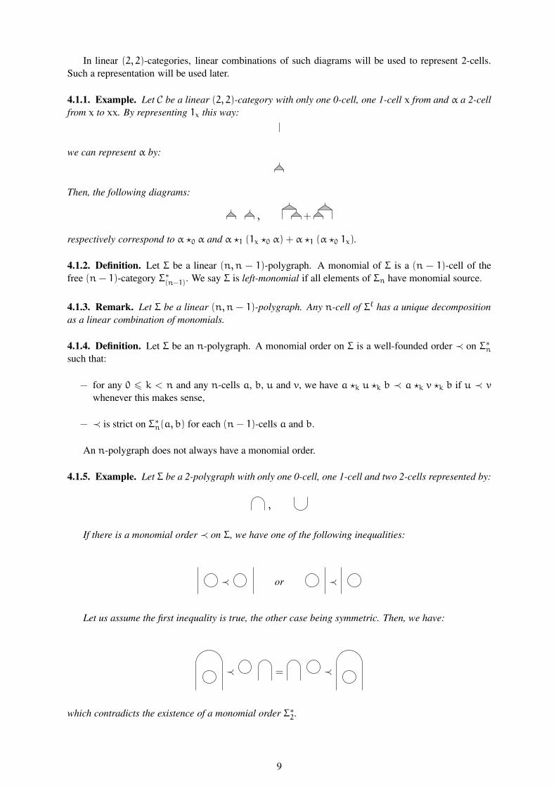
In linear (2, 2)-categories, linear combinations of such diagrams will be used to represent 2-cells.

Such a representation will be used later.

4.1.1. Example. Let C be a linear (2, 2)-category with only one 0-cell, one 1-cell x from and α a 2-cell

from x to xx. By representing 1x this way:

we can represent α by:

Then, the following diagrams:

, +

respectively correspond to α ⋆0 α and α ⋆1 (1x ⋆0 α) + α ⋆1 (α ⋆0 1x).

4.1.2. Definition. Let Σ be a linear (n,n − 1)-polygraph. A monomial of Σ is a (n − 1)-cell of the

free (n − 1)-category Σ∗(n−1)

. We say Σ is left-monomial if all elements of Σn have monomial source.

4.1.3. Remark. Let Σ be a linear (n,n − 1)-polygraph. Any n-cell of Σℓ has a unique decomposition

as a linear combination of monomials.

4.1.4. Definition. Let Σ be an n-polygraph. A monomial order on Σ is a well-founded order ≺ on Σ∗n

such that:

− for any 0 6 k < n and any n-cells a, b, u and v, we have a ⋆k u ⋆k b ≺ a ⋆k v ⋆k b if u ≺ v

whenever this makes sense,

− ≺ is strict on Σ∗n(a, b) for each (n − 1)-cells a and b.

An n-polygraph does not always have a monomial order.

4.1.5. Example. Let Σ be a 2-polygraph with only one 0-cell, one 1-cell and two 2-cells represented by:

,

If there is a monomial order ≺ on Σ, we have one of the following inequalities:

≺ or ≺

Let us assume the first inequality is true, the other case being symmetric. Then, we have:

≺ = ≺

which contradicts the existence of a monomial order Σ∗2.

9

4.2. Rewriting in linear (2, 2)-categories

We recall that a linear (2, 2)-category is a category enriched in linear categories. We will explicit

the rewriting systems arising from linear (3, 2)-polygraphs. A similar theory exists in the case of n-

polygraphs [GM09]. The rewriting theory of linear (2, 2)-categories we will present is a linear adaptation

of the case of 2-categories.

Let Σ be a linear (3, 2)-polygraph. The congruence generated by Σ is the equivalence relation ≡

on Σℓ2 such that u ≡ v if there is a 3-cell α in Σℓ such that s2(α) = u and t2(α) = v. Note that

in a linear (3, 2)-category, all 3-cells are invertible. if α is a 3-cell from a 2-cell u to a 2-cell v, the 3-

cell 1v+1u−α has 2-source v and 2-target u. Let Σ be a linear (3, 2)-polygraph. A linear (2, 2)-category

is presented by Σ if it is isomorphic to the quotient of Σℓ2 by the congruence generated by Σ.

We introduce next the notions of rewriting step of a left-monomial linear (3, 2)-polygraph to de-

fine branchings, termination and conflence in this context. We will fix Σ a left-monomial linear (3, 2)-

polygraph for the remainder of this section.

4.2.1. Definition. A rewriting step of Σ is a 3-cell of Σℓ of the form:

λm1 ⋆1 (m2 ⋆0 s2(α) ⋆0 m3) ⋆1 m4 + u ⇛ λm1 ⋆1 (m2 ⋆0 s2(α) ⋆0 m3) ⋆1 m4 + u

λ s2(α)

· · ·

· · ·

m3

· · ·

· · ·

m2

· · ·

· · ·

m1

· · ·

m4

· · ·

+ u ⇛ λ t2(α)

· · ·

· · ·

m3

· · ·

· · ·

m2

· · ·

· · ·

m1

· · ·

m4

· · ·

+ u

where α is in Σ3, the mi are monomials, λ is a nonzero scalar and u is a 2-cell such that the mono-

mial λm2⋆1 (m1αm4)⋆1m3 does not appear in the monomial decomposition of u. A rewriting sequence

of Σ is a finite or infinite sequence:

u0 ⇛ · · · ⇛ un ⇛ · · ·

of rewriting steps of Σ.

For any 2-cells u and v, we say u rewrites into v if there is a non-degenerate rewriting sequence from

u to v. A 2-cell is a normal form if it can not be rewritten. We say Σ is normalizing if each 2-cell rewrites

into a normal form or is a normal form.

A branching of Σ is a pair of rewriting sequences of Σ with the same 2-source:

u0

· · · ⇛ un ⇛ · · ·

· · · ⇛ u ′n ⇛ · · ·

A local branching of Σ is a pair of rewriting steps of Σ with the same 2-source.

10

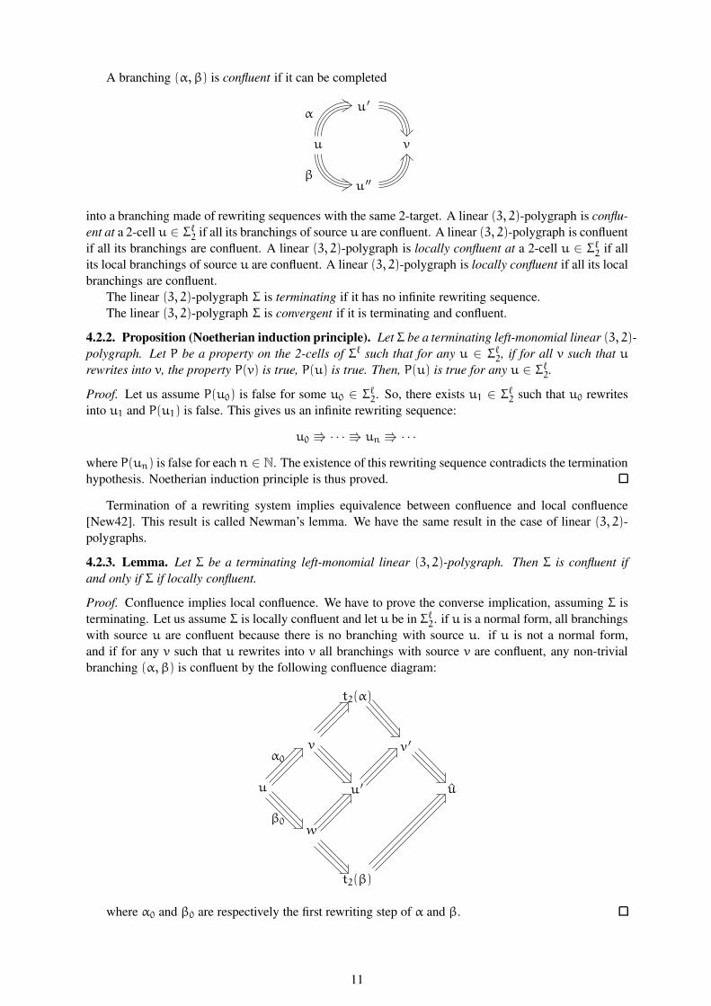
A branching (α,β) is confluent if it can be completed

u

u ′

u ′′

α

β

v

into a branching made of rewriting sequences with the same 2-target. A linear (3, 2)-polygraph is conflu-

ent at a 2-cell u ∈ Σℓ2 if all its branchings of source u are confluent. A linear (3, 2)-polygraph is confluent

if all its branchings are confluent. A linear (3, 2)-polygraph is locally confluent at a 2-cell u ∈ Σℓ2 if all

its local branchings of source u are confluent. A linear (3, 2)-polygraph is locally confluent if all its local

branchings are confluent.

The linear (3, 2)-polygraph Σ is terminating if it has no infinite rewriting sequence.

The linear (3, 2)-polygraph Σ is convergent if it is terminating and confluent.

4.2.2. Proposition (Noetherian induction principle). Let Σ be a terminating left-monomial linear (3, 2)-

polygraph. Let P be a property on the 2-cells of Σℓ such that for any u ∈ Σℓ2, if for all v such that u

rewrites into v, the property P(v) is true, P(u) is true. Then, P(u) is true for any u ∈ Σℓ2.

Proof. Let us assume P(u0) is false for some u0 ∈ Σℓ2. So, there exists u1 ∈ Σℓ

2 such that u0 rewrites

into u1 and P(u1) is false. This gives us an infinite rewriting sequence:

u0 ⇛ · · · ⇛ un ⇛ · · ·

where P(un) is false for each n ∈ N. The existence of this rewriting sequence contradicts the termination

hypothesis. Noetherian induction principle is thus proved.

Termination of a rewriting system implies equivalence between confluence and local confluence

[New42]. This result is called Newman’s lemma. We have the same result in the case of linear (3, 2)-

polygraphs.

4.2.3. Lemma. Let Σ be a terminating left-monomial linear (3, 2)-polygraph. Then Σ is confluent if

and only if Σ if locally confluent.

Proof. Confluence implies local confluence. We have to prove the converse implication, assuming Σ is

terminating. Let us assume Σ is locally confluent and let u be in Σℓ2. if u is a normal form, all branchings

with source u are confluent because there is no branching with source u. if u is not a normal form,

and if for any v such that u rewrites into v all branchings with source v are confluent, any non-trivial

branching (α,β) is confluent by the following confluence diagram:

u

vα0

t2(α)

wβ0

t2(β)

u ′

v ′

u

where α0 and β0 are respectively the first rewriting step of α and β.

11

This proof for linear (3, 2)-polygraphs by Noetherian induction works like in the case of abstract

rewriting systems [Hue80].

4.2.4. Definition. An aspherical branching of Σ is a branching made up of two identical rewriting steps.

A Peiffer branching is a branching of the form:

t2(α) ⋆1 s2(β) + h ⇚ s2(α) ⋆1 s2(β) + h ⇛ s2(α) ⋆1 t2(β) + h

where α and β are rewriting steps of Σ with monomial source. Note that all branchings of the form:

t2(α) ⋆1 s2(β) + h ⇚ s2(α) ⋆0 s2(β) + h ⇛ s2(α) ⋆1 t2(β) + h

are also Peiffer branchings beacause of the relation:

s2(α) ⋆0 s2(β) = (s2(α) ⋆0 1s1(β)) ⋆1 (1s1(α) ⋆0 s2(β))

An additive branching is a branching of the form:

t2(α) + s2(β) ⇚ s2(α) + s2(β) ⇛ s2(α) + t2(β)

where α and β are rewriting steps of Σ. An overlapping branching is a branching that is not aspherical,

Peiffer or additive.

4.2.5. Notation. Let us partition Σ3 in multiple families and assume an overlapping branching (α,β)

of Σ is confluent. If α is in the family i and β is in the family j, we denote:

u ⇛ij v

where u is the source of (α,β) and v is a 2-cell attained after completion of (α,β).

4.2.6. Definition. Let ⊑ be the order on the monomials of Σ such that we have f ⊑ g if we have g =

m1 ⋆1 (m2 ⋆0 f ⋆0 m3) ⋆1 m4 for some monomials mi. A critical branching is an overlapping branching

with monomial source such that its source is minimal for ⊑.

4.2.7. Definition. A 3-cell of Σℓ is elementary if it is of the form λm1 ⋆1 (m2 ⋆0 α ⋆0 m3) ⋆1 m4 + u

where α is in Σ3, the mi are monomials, λ is a nonzero scalar, and u is a 2-cell.

4.2.8. Example. Let A and B be two monomials of Σℓ such that there is a rewriting step from A to B.

Then, there is a 3-cell of Σℓ from 2A to A+B which is not a rewriting step. But this 3-cell is elementary.

4.2.9. Lemma. Let α be an elementary 3-cell. Then, there exists two rewriting sequences β and γ of

length at most 1 such that α = β ⋆2 γ−1.

Proof. Let us write α = α ′+g where α ′ is a rewriting step from a 2-cell u to a 2-cell f and g is a 2-cell.

Let us write g = λu+h where f does not appear in the monomial decomposition of h. Then, (λ+1)u+h

rewrites into (λ+ 1)f+ h either by an identity or a rewriting step and u+ g rewrites into (λ+ 1)u+ h

either by an identity or a rewriting step.

4.2.10. Definition. Let Σ be a left-monomial linear (3, 2)-polygraph. The rewrite order of Σ is the

relation 4 ′Σ on Σℓ

2 defined by v 4 ′Σ u if u rewrites into v or u = v. The canonical rewrite order of Σ is

the minimal binary relation 4Σ such that:

− if v 4 ′Σ u, then v 4Σ u,

− if v 4Σ u, v ′ 4Σ u ′, and u and u ′ do not have any common monomial in their decomposition,

then v+ v ′ 4Σ u+ u ′.

The strict canonical rewrite order of Σ is the strict order ≺Σ defined for any 2-cells u and v by v ≺Σ u

if we have v 4Σ u but not u 4Σ v. The semistrict rewrite order of Σ is the binary relation ≺ ′Σ on Σℓ

2

defined by v ≺ ′Σ u if u rewrites into v.

12

4.2.11. Remark. if Σ is terminating, those relations are order relations and ≺Σ is well-founded. In

general, only ≺Σ is an order.

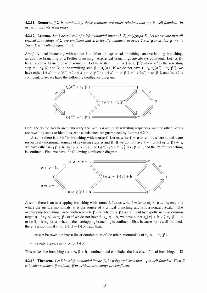
4.2.12. Lemma. Let f be a 2-cell of a left-monomial linear (3, 2)-polygraph Σ. Let us assume that all

critical branchings of Σ are confluent and Σ is locally confluent at every 2-cell g such that g ≺Σ f.

Then, Σ is locally confluent at f.

Proof. A local branching with source f is either an aspherical branching, an overlapping branching,

an additive branching or a Peiffer branching. Aspherical branchings are always confluent. Let (α,β)

be an additive branching with source f. Let us write f = s2(α′) + s2(β

′) where α ′ is the rewriting

step α − s2(β) and β ′ is the rewriting step β − s2(α). If we do not have f ≺Σ t2(α′) + t2(β

′), we

have either t2(α′) + s2(β

′) 4 ′Σ s2(α

′) + t2(β′) or s2(α

′) + t2(β′) 4 ′

Σ t2(α′) + s2(β

′), and (α,β) is

confluent. Else, we have the following confluence diagram:

f

α

β

t2(α′) + s2(β

′)

s2(α′) + t2(β

′)

t2(α′) + t2(β

′)

f ′

f ′′

f

a

b

Here, the dotted 3-cells are elementary, the 3-cells a and b are rewriting sequences, and the other 3-cells

are rewriting steps or identities, whose existence are guaranteed by Lemma 4.2.9.

Assume there is a Peiffer branching with source f. Let us write f = u ⋆1 v + h where u and v are

respectively monomial sources of rewriting steps α and β. If we do not have f ≺Σ t2(α) ⋆1 t2(β) + h,

we have either u ⋆1 β+h 4 ′Σ t2(α) ⋆1 v+h or t2(α) ⋆1 v+h 4 ′

Σ u ⋆1 β+h, and the Peiffer branching

is confluent. Else, we have the following confluence diagram:

f

α ⋆1 v + h

u ⋆1 β+ h

t2(α) ⋆1 v+ h

u ⋆1 t2(β) + h

t2(α) ⋆1 t2(β) + h

f ′

f ′′

f

a

b

Assume there is an overlapping branching with source f. Let us write f = λm1(m2 ⋆1 u ⋆1 m3)m4 + h

where the mi are monomials, u is the source of a critical branching and λ is a nonzero scalar. The

overlapping branching can be written (α+h,β+h) where (α,β) is confluent by hypothesis to a common

target g. if t2(α) = t2(β) or if we do not have f ≺Σ g + h, we have either t2(α) + h 4 ′Σ t2(β) + h

or t2(β)+h 4 ′Σ t2(α)+h, and the overlapping branching is confluent. Else, because ≺Σ is well-founded,

there is a monomial m of t2(α) − t2(β) such that:

− m can be rewritten into a linear combination of the others monomials of t2(α) − t2(β),

− m only appears in t2(α) or t2(β).

This makes the branching (α+ h,β+ h) confluent and concludes the last case of local branching.

4.2.13. Theorem. Let Σ be a left-monomial linear (3, 2)-polygraph such that ≺Σ is well-founded. Then, Σ

is locally confluent if and only if its critical branchings are confluent.

13

Proof. if Σ is locally confluent, then its critical branchings are confluent. Conversely, let us assume that

all critical branchings of Σ are confluent. Induction on ≺Σ can be used to prove that Σ is confluent.

Indeed, Σ is locally confluent at every minimal 2-cell for ≺Σ and lemma 4.2.12 concludes the proof.

4.2.14. Lemma. Let Σ be a confluent left-monomial linear (3, 2)-polygraph. Let C be the linear (2, 2)-

category presented by Σ. Then, for any 1-cells u and v of C with same 0-source and 0-target, the linear

map τ from Σℓ2(u, v) to C(u, v) sending each 2-cell to its congruence class has for kernel the subspace

of Σℓ2(u, v) made of all 2-cells having 0 as a normal form.

Proof. Σ being left-monomial, 0 is a normal form. If a 2-cell rewrites into 0, it is congruent to 0.

Converesly, let us assume a non-zero 2-cell f is in Ker(τ). Confluence of Σ makes f rewrite into 0. This

concludes the proof.

4.2.15. Proposition. Let Σ be a confluent and normalizing left-monomial linear (3, 2)-polygraph. Let

C be the linear (2, 2)-category presented by Σ. Then, for any 1-cells u and v of C with same 0-source

and 0-target, the set of monomials of Σ in normal form with 1-source u and 1-target v gives a basis of

C(u, v).

Proof. Let us fix two 1-cells u and v of C with same 0-source and 0-target. Every 2-cell of Σℓ with

1-source u and 1-target v has a normal form because Σ is terminating. Each normal form is a linear

combination of monomials in normal form because Σ is left-monomial. So, the family of monomials

in normal form is generating. The family of monomials in normal forms is free because Σ is confluent,

which allows us to use lemma 4.2.14. This concludes the proof.

4.3. Confluence by decreasingness

We fix in this section Σ a left-monomial linear (3, 2)-polygraph.

4.3.1. Definition. Let R be the set of all rewriting steps of Σ. We say Σ is decreasing if there is a well-

founded order ≺ on a partition P of R such that, for every I and J in P, every local branching (i, j)

with i ∈ I and j ∈ J can be completed into a confluence diagram

j

i

aI

bJ

c

aJ bI c ′

such that:

− aI is a rewriting sequence such that for each rewriting step k in aI, there exists K in P such

that k ∈ K and K ≺ I.

− aJ is a rewriting sequence such that for each rewriting step k in aJ, there exists K in P such

that k ∈ K and K ≺ J.

− bI is either an identity or an element of I.

− bJ is either an identity or an element of J.

− c and c ′ are rewriting sequences such that for each rewriting step k in c or c ′, there exists K in P

such that k ∈ K and K ≺ I or K ≺ J.

14

4.3.2. Example. Let Σex be the linear (3, 2)-polygraph with only one 0-cell, one 1-cell a, two 2-cells

represented by:

,

and the following 3-cell:

⇛

A 2-cell is said in semi-normal form if it cannot be rewritten by using a rewriting step of one of the

following forms:

⇛ , ⇛

We give a partition {Pn|n ∈ N} of the set of rewriting steps of Σex such that, for any rewriting step α, we

have α ∈ Pn if the shortest rewriting sequence from t2(α) to a semi-normal form is of length n. This is

a partition of the set of rewriting steps of Σex because every 2-cell rewrites into a semi-normal form. We

define on {Pn|n ∈ N} the order ≺ by Pn ≺ Pm if n < m. With this well-ordered partition given, Σex is

decreasing. This translates the fact any 2-cell has a unique semi-normal form.

The following result is proved in [vO94] in the case of abstract rewriting systems. The proof can be

adapted to the case of linear (3, 2)-polygraphs.

4.3.3. Theorem. Let Σ be a left-monomial libear (3, 2)-polygraph. if Σ is decreasing, then Σ is conflu-

ent.

Proof. Let us assume Σ is decreasing for a partition P of the set of its rewriting steps and an order ≺

on P. We introduce the following map | · · · | from the free monoid P∗ over P to NP :

− if ε is the empty word of P∗, for every K in P, we have |ε|(K) = 0,

− for every I in P and every K in P, we have |I|(I) = 1 and |I|(K) = 0 if I 6= K,

− for every I in P and every word σ of P∗, we have |Iσ| = |I|+ |σ(I)| where σ(I) denotes the word σ

without the letters J such that J ≺ I.

We remark that for every words σ1 and σ2 of P∗, we have:

|σ1σ2| = |σ1| + |σ2|(σ1),

where:

|σ2|(σ1)(K) =

{0 if there exists I in P such that K ≺ I and |σ1|(I) 6= 0

|σ2|(K) otherwise

Then, we extend | · · · | to the set of finite rewriting sequences of Σ by defining |r1 · · · rn| = |K1 · · ·Kn|

for every rewriting sequence

u0 ⇛r1

· · · ⇛rn

un

such that for each 1 6 i 6 n we have ri ∈ Ki.

We extend finally | · · · | to the set of branchings of Σ made of finite rewriting sequences by defin-

ing |(α,β)| = |α| + |β| for every finite rewriting sequences α and β.

We now define a strict order ≺ ′ on NP . For any M and N in N

P , we define M ≺ ′ N if there

exist X, Y and Z in NP such that:

15

− M = Z+ X,

− N = Z+ Y,

− Y is not zero,

− for every I in P such that M(I) 6= 0, there exists J in P such that N(J) 6= 0 and I ≺ J.

The order ≺ ′ is well-founded because ≺ is. We call 4 ′ the symmetric closure of ≺ ′.

To prove that Σ is confluent, it is sufficient to prove that every branching (α,β) made of finite

rewriting sequences can be completed into a confluence diagram (α ⋆2 τ, β ⋆2 σ)

β

α

τ

σ

such that:

|α ⋆2 τ| 4′ |(α,β)|, (6)

|β ⋆2 σ| 4′ |(α,β)|. (7)

We will prove this fact by induction on |(α,β)|. This is trivial when |(α,β)| is minimal because this is

the case of a trivial branching made of two identities.

Let us now assume that for each branching (α ′, β ′)made of finite rewriting sequences such that |(α ′, β ′)| ≺ ′

|(α,β)|, we can complete (α ′, β ′) into a confluence diagram verifying (6) and (7). For every diagram of

the following form:

δ0

γ1

δ1

τ

γ2

such that |γ1 ⋆2 δ1| 4′ |(δ0, γ1)|, we have |(δ1, γ2)| ≺

′ |(δ0, γ1 ⋆2 γ2)| if γ1 is not an identity. Indeed:

|(δ1, γ2)| ≺′ |γ1|+ |(δ1, γ2)|

(γ1) = |γ1 ⋆2 δ1|+ |γ2|(γ1) 4

′ |(δ0, γ1)| + |γ2|(γ1) = |(δ0, γ1 ⋆2 γ2)|.

Let us also remark that for every diagram of the form:

δ0

γ1

δ1

τ1

γ2

δ2

τ2

such that:

− |δ0 ⋆2 τ1| 4′ |(δ0, γ1)| and |γ1 ⋆2 δ1| 4

′ |(δ0, γ1)|,

− |δ1 ⋆2 τ2| 4′ |(δ1, γ2)| and |γ2 ⋆2 δ2| 4

′ |(δ1, γ2)|

We have the pasting property |δ0 ⋆2 τ1 ⋆2 τ2| 4′ |(δ0, γ1 ⋆2 γ2)| and |γ1 ⋆2 γ2 ⋆2 δ2| 4

′ |(δ0, γ1 ⋆2 γ2)|.

Indeed:

|δ0 ⋆2 τ1 ⋆2 τ2| = |δ0 ⋆2 τ1| + |τ2|(δ0⋆2τ1) 4

′ |(δ0, γ1)| + |τ2|(δ0⋆2τ1)(γ1) 4

′ |(δ0, γ1 ⋆2 γ2)|,

16

|γ1 ⋆2 γ2 ⋆2 δ2| = |γ1 ⋆2 γ2| + |δ2|(γ1)(γ2) 4

′ |γ1 ⋆2 γ2| + |δ2|(γ2) 4

′ |(δ0, γ1 ⋆2 γ2)|.

To prove (α,β) is confluent when α and β have nonzero length, we consider α0 the first step of α

and β0 the first step of β. We have then the following confluence diagram:

IH1α0

t2(α)

β0

t2(β)

D

IH2

Where D verifies (6) and (7) by decreasingness of Σ, the diagram IH1 exists because of the induction

hypothesis and verifies (6) and (7) by the pasting property. Finally, the induction hypothesis allows us to

construct IH2. The pasting property proves all the diagram verifies (6) and (7). This proves in particular

by well-founded induction Σ is confluent.

4.3.4. Example. The linear (3, 2)-polygraph Σex from 4.3.2 is decreasing and is therefore confluent.

Because every 2-cell rewrites into a semi-normal form and the semi-normal form of a 2-cell is unique,

we easily conclude Σex is indeed confluent.

5. THE AFFINE ORIENTED BRAUER CATEGORY

5.1. Dotted oriented Brauer diagrams with bubbles

After recalling the definition of the affine oriented Brauer category AOB from [BCNR14], we will

present it by a linear (3, 2)-polygraph.

5.1.1. Dotted oriented Brauer diagrams with bubbles. A dotted oriented Brauer diagram with bub-

bles is a planar diagram such that:

− edges are oriented,

− edges are either bubbles or have a boundary as source and target,

− each edge is decorated with an arbitrary number of dots not allowed to pass through the crossings.

5.1.2. Equivalence of dotted oriented Brauer diagrams with bubbles. Two dotted oriented Brauer

diagrams are equivalent if one can be transformed into the other with isotopies and Reidemeister moves.

A description of those moves can be found in [Tur10]. An isotopy can move a dot along an edge but

cannot make a dot go through a crossing. A dotted oriented Brauer diagram is normally ordered if:

− all bubbles are clockwise,

− all bubbles are in the leftmost side region,

− all dots are either on a bubble or a segment pointing toward a boundary.

17

5.1.3. Example. Here is an example of dotted oriented Brauer diagram:

This diagram is not normally ordered. The following one is normally ordered:

Those diagrams are not equivalent.

Dotted oriented Brauer diagrams with bubbles will be described as 2-cells of a 2-category with ver-

tical and horizontal concatenation respectively standing as 1-composition and 0-composition.

5.1.4. Definition. The affine oriented Brauer category AOB is the linear (2, 2)-category with one 0-

cell, two generating 1-cells and with 2-cells from a to b given by linear combinations of dotted oriented

Brauer diagrams with bubbles with source a and target b subject to the following relations:

− invariance by equivalence given in 5.1.2,

−

= +

5.1.5. An equational presentation of AOB. There is a presentation by generators and relations of the

linear (2, 2)-category AOB given in [BCNR14]. The category AOB is the linear (2, 2)-category with

only one 0-cell, two generating 1-cells ∧ and ∨ and five generating 2-cells

1c⇒ ∧∨, ∨∧

d⇒ 1, ∧∧s⇒ ∧∧, ∧∨

t⇒ ∨∧, ∧x⇒ ∧

respectively represented by:

, , , ,

subject to the following relations:

= =

= = = +

= =

From this equational presentation of the linear (2, 2)-category AOB, we deduce a linear (3, 2)-

polygraph presenting AOB.

18

5.1.6. The linear (3, 2)-polygraph AOB. Let us define the linear (3, 2)-polygraph AOB. It is the (3, 2)-

polygraph with only one 0-cell and:

− AOB1 = {∧,∨},

− AOB2 ={

, , , ,}

,

− AOB3 is made of the following 3-cells:

⇛ ⇛

⇛ ⇛ ⇛ +

⇛ ⇛

This linear (3, 2)-polygraph presents the linear (2, 2)-category AOB. This presentation is not con-

fluent. For example, the following critical branching is not confluent:

⇚ ⇛ +

We will give a confluent presentation of the linear (2, 2)-category AOB in Theorem 5.2.9.

5.2. A confluent presentation of AOB

We will give a linear (3, 2)-polygraph AOB presenting the linear (2, 2)-category AOB, with more 2-cells

than the linear (3, 2)-polygraph AOB. We will prove that AOB is confluent. The presence of redundant 2-

cells can be seen as an addition of redundant generators to give more relations and make our presentation

confluent.

5.2.1. The linear (3, 2)-polygraph AOB. The linear (3, 2)-polygraph is defined by:

− AOB has the same 0-cells and 1-cells than the linear (3, 2)-polygraph AOB,

− AOB2 = AOB2 ∪{

, , , ,}

,

− AOB3 is made of the following four families of 3-cells:

19

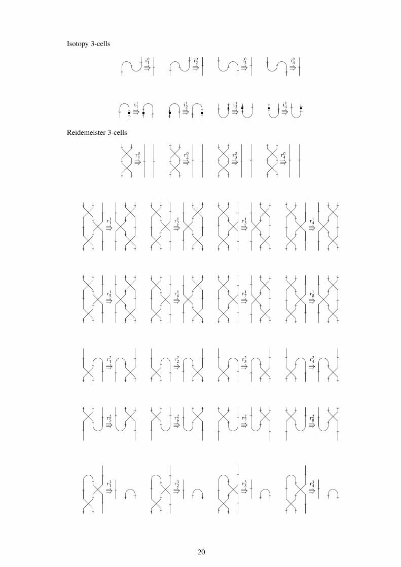
Isotopy 3-cells

i01⇛

i02⇛

i03⇛

i04⇛

i11⇛

i12⇛

i13⇛

i14⇛

Reidemeister 3-cells

r01⇛

r02⇛

r03⇛

r04⇛

r11⇛

r12⇛

r13⇛

r14⇛

r15⇛

r16⇛

r17⇛

r18⇛

r21⇛

r22⇛

r23⇛

r24⇛

r25⇛

r26⇛

r27⇛

r28⇛

r31⇛

r32⇛

r33⇛

r34⇛

20

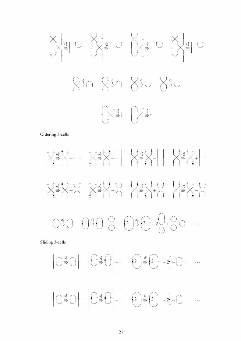
r35⇛

r36⇛

r37⇛

r38⇛

r41⇛

r42⇛

r43⇛

r44⇛

r51⇛

r52⇛

Ordering 3-cells

o01⇛ +

o02⇛ −

o03⇛ −

o04⇛ +

o05⇛ −

o06⇛ +

o07⇛ +

o08⇛ −

o10⇛

o11⇛ − 2

o12⇛ 2 − 2 + · · ·

Sliding 3-cells

s00⇛

s01⇛ + 2

s02⇛ 2 + 2 + · · ·

s10⇛

s11⇛ − 2

s12⇛ 2 − 2 − · · ·

21

5.2.2. Remark. The last three families of 3-cells correspond to infinite families of relations which can

be calculated by induction. Those relations are noted as in Convention (5). The first induction formula

is given in [BCNR14]. If we denote the counterclockwise bubble with n dots

n

as un,0 and by expressing the clockwise bubbles with m dots

m

as u0,m, we have for any n and m of N:

un+1,m = un,m+1 − un,0 ⋆1 u0,m.

Which can be used to rewrite un,0 as a linear combination of the family (uj0,i)06i6n,j∈N. The others

induction forumulas are:

vn+1,m = vn,m+1 +wn+m +

n−1∑

k=0

wm+n−k ⋆1 vk,0,

v ′n+1,m = v ′

n,m+1 +w ′n+m −

n−1∑

k=0

v ′0,k ⋆1 w

′m+n−k

where vn,0, v0,m, v ′n,0 and v ′

0,m respectively denote:

n , m , n , m

and where wn and w ′n respectively denote:

n , n

Let us now expand on the first chapter of [Tur10]. This chapter defines first ribbon categories as

braided monoidal categories with duals and twist. The twist is a natural transformation θ from the

identity functor to itself satisfying:

θV⊗W = bW,V ◦ (θV ⊗ θW) ◦ bV,W

for each objects V and W, where b denotes the braiding. A ribbon category satisfies the axiom θ∗ = θ.

An example of ribbon category is the category of ribbon tangles on a set S of colors. This strict

monoidal category RIBS is defined by:

− the objects of RIBS are the words of the free monoid on S× {∨,∧},

− the morphisms of RIBS from a word u to a word v are the oriented tangles of colored ribbons

such that the word u is on the upper boundary and the word v is on the lower boundary,

− two isotopic tangles are equal.

22

In this category, each object is its own dual. The twist corresponds to transversally twisting a ribbon

by 360 degrees. Turaev then gives a presentation by generators and relations of RIBS. The genera-

tors are the cups, caps, crossings and twistings of each ribbon colors and directions. The relations are

invariance by multiple moves Turaev describes as elementary isotopies and Reidemeister moves.

From the presentation of RIBS by generators and relations, we can present the category RIB of

ribbon tangles with only one color by generators and relations. RIB being a monoidal category, we can

describe it as a 2-category with only one 0-cell. The linearization of RIB is thus a linear (2, 2)-category

with the same 0-cell and 1-cells than RIB. We will call RIBK this linear (2, 2)-category, where K is

our fixed field. Let OB be the subcategory of AOB defined by:

− OB0 = AOB0 and OB1 = AOB1,

− OB2 is made of the oriented Brauer diagrams with bubbles (without dots)

The linear 2-functor from RIBK to OB sending each ribbon to a string with the same direction is full

as noted in [BCNR14]. We derive from this fact a description of elementary isotopies and Reidemeister

moves first described in [Tur10] for the linear (2, 2)-category AOB

5.2.3. Proposition. The linear (3, 2)-polygraph AOB is a presentation of the linear (2, 2)-category AOB.

Proof. All 3-cells of AOB correspond to a relation verified in the linear (2, 2)-category AOB by Defini-

tion 5.1.4. Moreover, the set of 3-cells of type i0, r0, r1, r2, r4, and r5 contains all elementary isotopies

and Reidemeister moves given in [Tur10] (Chapter 1, Section 4), and thus generates the equivalence of

dotted oriented Brauer diagram with bubbles. As a consequence, the 3-cells of AOB are sufficient to find

any relation verified in AOB.

Then, we define some particular 2-cells of AOBℓ2.

5.2.4. Definition. We call a monomial of AOB quasi-reduced if the only 3-cells we can apply to it are

of the form:

i ⇛ i − 1

⇛ ⇛ +

2

⇛ 2 + 2 + · · ·

⇛ ⇛ −

2

⇛ 2 + 2 + · · ·

⇛ ⇛ −2

⇛ 2 + 2 + · · ·

⇛ ⇛ +2

⇛2 + 2 + · · ·

23

We call a 2-cell of AOBℓ2 quasi-reduced if all monomials in its monomial decomposition are quasi-

reduced.

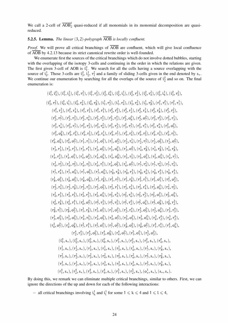
5.2.5. Lemma. The linear (3, 2)-polygraph AOB is locally confluent.

Proof. We will prove all critical branchings of AOB are confluent, which will give local confluence

of AOB by 4.2.13 because its strict canonical rewrite order is well-founded.

We enumerate first the sources of the critical branchings which do not involve dotted bubbles, starting

with the overlapping of the isotopy 3-cells and continuing in the order in which the relations are given.

The first given 3-cell of AOB is i01. We search for all the cells having a source overlapping with the

source of i10. Those 3-cells are i03, i12, r21 and a family of sliding 3-cells given in the end denoted by s∗.

We continue our enumeration by searching for all the overlaps of the source of i02 and so on. The final

enumeration is:

(i01, i03), (i

01, i

12), (i

01, r

21), (i

01, r

23), (i

02, i

04), (i

02, i

13), (i

02, r

22), (i

02, r

24), (i

03, i

14), (i

03, r

25),

(i03, r27), (i

04, i

11), (i

04, r

26), (i

04, r

28), (i

11, r

22), (i

11, r

24), (i

13, r

26), (i

13, r

28), (r

01, r

01), (r

01, r

11),

(r01, r12), (r

01, r

14), (r

01, r

21), (r

01, r

31), (r

02, r

02), (r

02, r

12), (r

02, r

14), (r

02, r

18), (r

02, r

22),

(r02, r27), (r

02, r

33), (r

02, r

36), (r

02, r

42), (r

02, r

43), (r

02, o

06), (r

02, o

07), (r

03, r

03), (r

03, r

13),

(r03, r16), (r

03, r

17), (r

03, r

23), (r

03, r

26), (r

03, r

32), (r

03, r

37), (r

03, r

41), (r

03, r

44), (r

03, o

05),

(r03, o08), (r

04, r

04), (r

04, r

15), (r

04, r

16), (r

04, r

17), (r

04, r

24), (r

04, r

25), (r

04, r

34), (r

04, r

35),

(r04, o04), (r

04, o

07), (r

11, r

11), (r

11, o

01), (r

11, o

02), (r

12, r

14), (r

12, r

37), (r

12, o

05), (r

12, o

07),

(r13, r13), (r

13, r

32), (r

13, r

41), (r

13, o

05), (r

13, o

06), (r

13, o

07), (r

14, r

28), (r

14, r

28), (r

14, r

38),

(r14, r42), (r

14, o

01), (r

14, o

02), (r

14, o

06), (r

14, o

08), (r

15, r

15), (r

15, o

03), (r

15, o

04), (r

16, r

17),

(r16, r23), (r

16, r

25), (r

16, r

35), (r

16, r

41), (r

16, o

05), (r

16, o

07), (r

17, r

24), (r

17, r

26), (r

17, r

34),

(r17, r44), (r

17, o

04), (r

17, o

05), (r

17, o

06), (r

18, r

18), (r

18, r

33), (r

18, r

36), (r

18, r

42), (r

18, r

43),

(r18, o03), (r

18, o

05), (r

18, o

08), (r

21, r

28), (r

21, r

37), (r

21, r

38), (r

21, r

51), (r

21, o

01), (r

21, o

02),

(r22, r34), (r

22, r

38), (r

22, r

43), (r

22, o

05), (r

23, r

31), (r

23, r

36), (r

23, r

44), (r

23, o

06), (r

24, r

25),

(r24, r33), (r

24, r

35), (r

24, r

52), (r

24, o

04), (r

25, r

34), (r

25, r

36), (r

25, r

52), (r

25, o

03), (r

25, o

04),

(r26, r38), (r

26, r

41), (r

26, o

07), (r

27, r

33), (r

27, r

35), (r

27, r

42), (r

27, o

06), (r

27, o

08), (r

28, r

32),

(r28, r51), (r

28, o

02), (r

31, r

38), (r

31, o

01), (r

31, o

02), (r

32, r

44), (r

32, o

05), (r

32, o

06), (r

33, r

43),

(r33, o03), (r

33, o

05), (r

34, r

35), (r

34, o

05), (r

34, o

07), (r

35, o

03), (r

35, o

04), (r

36, r

42), (r

36, r

42),

(r36, o07), (r

36, o

08), (r

37, r

41), (r

37, o

01), (r

37, o

07), (r

38, o

05), (r

38, o

07), (r

41, r

44), (r

41, o

06),

(r42, r43), (r

42, o

05), (r

43, o

08), (r

44, o

07), (r

51, o

01), (r

52, o

03),

(i01, s∗), (i02, s∗), (i

03, s∗), (i

04, s∗), (r

01, s∗), (r

02, s∗), (r

03, s∗), (r

04, s∗),

(r11, s∗), (r12, s∗), (r

13, s∗), (r

14, s∗), (r

15, s∗), (r

16, s∗), (r

17, s∗), (r

18, s∗),

(r21, s∗), (r22, s∗), (r

23, s∗), (r

24, s∗), (r

25, s∗), (r

26, s∗), (r

27, s∗), (r

28, s∗),

(r31, s∗), (r32, s∗), (r

33, s∗), (r

34, s∗), (r

35, s∗), (r

36, s∗), (r

37, s∗), (r

38, s∗),

(r41, s∗), (r42, s∗), (r

43, s∗), (r

44, s∗), (r

51, s∗), (r

52, s∗), (o

1∗, s∗), (s∗, s∗).

By doing this, we remark we can eliminate multiple critical branchings, similar to others. First, we can

ignore the directions of the up and down for each of the following interactions:

− all critical branchings involving i1k and i1l for some 1 6 k 6 4 and 1 6 l 6 4,

24

− all critical branchings involving i1k for some 1 6 k 6 4 and a Reidemeister 3-cell,

− all critical branchings involving two Reidemeister 3-cells.

Indeed, the above 3-cells correspond to the relations verified by the category OB defined in [BCNR14].

Those relations do not depend on the up or down directions. Those relations are also invariant by axial

symmetry. Those facts allow us to withdraw multiple critical pairs from our enumeration. In the same

way, any critical branchings involving two isotopy 3-cells can be studied up to axial symmetry.

The interactions between an ordering 3-cell and a Reidemester 3-cell are not invariant by symmetry.

But, when a critical branching involving an ordering 3-cell and a Reidemeister 3-cell rkl is confluent, all

critical branchings involving an ordering 3-cell and a 3-cell of the form rk∗ are confluent. This fact allows

us to treat multiple cases of critical branching simultaneously.

We now verify each critical branching is confluent. For each critical branching we are treating, we

will use notation 4.2.5. Thus, we will give the source of each critical branching and a target attained once

a confluence diagram is given for this critical pair.

⇛i0∗

i0∗

⇛i0∗

i1∗

⇛i0∗

s∗ ⇛i0∗

r2∗

⇛i1∗

r2∗

+ ⇛r0∗

r1∗

⇛r0∗

r2∗

⇛r0∗

r3∗

⇛r0∗

r4∗

⇛r0∗

o0∗

⇛r0∗

s∗ ⇛r1∗

r1∗

⇛r1∗

r2∗

⇛r1∗

r4∗

⇛r1∗

o0∗

+ + ⇛r1∗

s∗

25

⇛r2∗

r2∗

⇛r2∗

r3∗

⇛r2∗

r3∗

⇛r2∗

r3∗

⇛r2∗

r4∗

⇛r2∗

r5∗

⇛r2∗

o0∗

+ ⇛r2∗

s∗ ⇛r3∗

r3∗

⇛r3∗

r4∗

⇛r3∗

o0∗

⇛r3∗

s∗ ⇛r4∗

o0∗

⇛r4∗

s∗ ⇛r5∗

o0∗

⇛r5∗

s∗ ⇛o0∗

o0∗

⇛o1∗

s∗ ⇛s∗s∗

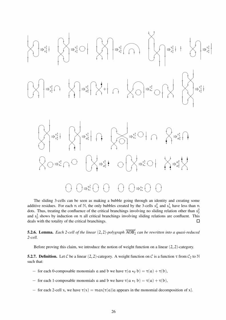
The sliding 3-cells can be seen as making a bubble going through an identity and creating some

additive residues. For each n of N, the only bubbles created by the 3-cells s0n and s1n have less than n

dots. Thus, treating the confluence of the critical branchings involving no sliding relation other than s00and s10 shows by induction on n all critical branchings involving sliding relations are confluent. This

deals with the totality of the critical branchings.

5.2.6. Lemma. Each 2-cell of the linear (2, 2)-polygraph AOBℓ2 can be rewritten into a quasi-reduced

2-cell.

Before proving this claim, we introduce the notion of weight function on a linear (2, 2)-category.

5.2.7. Definition. Let C be a linear (2, 2)-category. A weight function on C is a function τ from C2 to N

such that:

− for each 0-composable monomials a and b we have τ(a ⋆0 b) = τ(a) + τ(b),

− for each 1-composable monomials a and b we have τ(a ⋆1 b) = τ(a) + τ(b),

− for each 2-cell x, we have τ(x) = max{τ(a)|a appears in the monomial decomposition of x}.

26

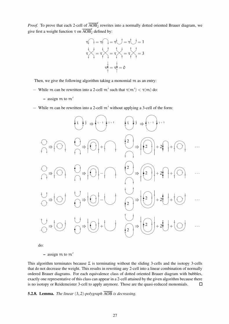
Proof. To prove that each 2-cell of AOBℓ2 rewrites into a normally dotted oriented Brauer diagram, we

give first a weight function τ on AOBℓ2 defined by:

τ = τ = τ = τ = 1

τ = τ = τ = τ = 3

τ = τ = 0

Then, we give the following algorithm taking a monomial m as an entry:

− While m can be rewritten into a 2-cell m ′ such that τ(m ′) < τ(m) do:

– assign m to m ′

− While m can be rewritten into a 2-cell m ′ without applying a 3-cell of the form:

i j ⇛i − 1 j + 1 i j ⇛

i − 1 j + 1

⇛ ⇛ +

2

⇛ 2 + 2 + · · ·

⇛ ⇛ −

2

⇛ 2 + 2 + · · ·

⇛ ⇛ −2

⇛ 2 + 2 + · · ·

⇛ ⇛ +2

⇛ 2 + 2 + · · ·

do:

– assign m to m ′

This algorithm terminates because Σ is terminating without the sliding 3-cells and the isotopy 3-cells

that do not decrease the weight. This results in rewriting any 2-cell into a linear combination of normally

ordered Brauer diagrams. For each equivalence class of dotted oriented Brauer diagram with bubbles,

exactly one representative of this class can appear in a 2-cell attained by the given algorithm because there

is no isotopy or Reidemeister 3-cell to apply anymore. Those are the quasi-reduced monomials.

5.2.8. Lemma. The linear (3, 2)-polygraph AOB is decreasing.

27

Proof. We define the set P = {Pn|n ∈ N} where for each rewriting step α of AOB and each n in N, we

have α ∈ Pn if and only if the rewriting sequence of minimal length from t2(α) to a quasi-reduced 2-cell

is of length n. Because of the fact that every 2-cell can be rewritten into a quasi-reduced one 5.2.6, P is a

partition of the set of rewriting steps of AOB. We give on this partition the order ≺ such that Pn ≺ Pm if

and only if n < m. This well-founded order respects all the properties of 4.3.1 for the critical branchings

of AOB. The decreasingness critical branchings is explicited in the appendix. Then, the order ≺ meets

the properties of 4.3.1, ending the proof by 4.3.3.

5.2.9. Theorem. The linear (3, 2)-polygraph AOB is a confluent presentation of AOB.

Proof. The linear (3, 2)-polygraph AOB is locally confluent by lemma 5.2.5. Lemma 5.2.8 allows us to

use 4.3.3 and conclude the proof.

This theorem implies the following result from [BCNR14]:

5.2.10. Corollary. Let a and b be two 1-cells of the linear (2, 2)-category AOB. Then, the vector

space AOB2(a, b) has basis given by equivalence classes of normally ordered dotted oriented Brauer

diagrams with bubbles with source a and target b.

Proof. We need to give a confluent left-monomial linear (3, 2)-polygraph presenting the linear (2, 2)-

category AOB such that:

− There is a bijection between the 2-cells of the free linear (2, 2)-category and dotted oriented Brauer

diagrams with bubbles.

− A normally ordered dotted oriented Brauer diagram does not rewrite into a linear combination of

non-equivalent others.

− Each 2-cell that is not in normal form rewrites into a linear combination of normally ordered dotted

oriented Brauer diagrams.

The linear (3, 2)-polygraph AOB from 5.2.9 verifies those properties. To prove that a normally

ordered Brauer diagram does not rewrite into a linear combination of non-equivalent others, it is sufficient

to show that a quasi-reduced 2-cell does not rewrite into another quasi-reduced 2-cell. The only way to

rewrite a quasi-reduced monomial is to apply sliding 3-cells or isototpy relations that do not decrease the

weight. So, the only way to rewrite a quasi-reduced monomial into a linear combination of others is to

use rewriting paths of the forms:

⇛ ⇛ ⇛ ⇛ · · ·

⇛ ⇛ ⇛ + ⇛ · · ·

⇛ ⇛ ⇛ − ⇛ · · ·

⇛ ⇛ ⇛ − ⇛ · · ·

28

⇛ ⇛ ⇛ + ⇛ · · ·

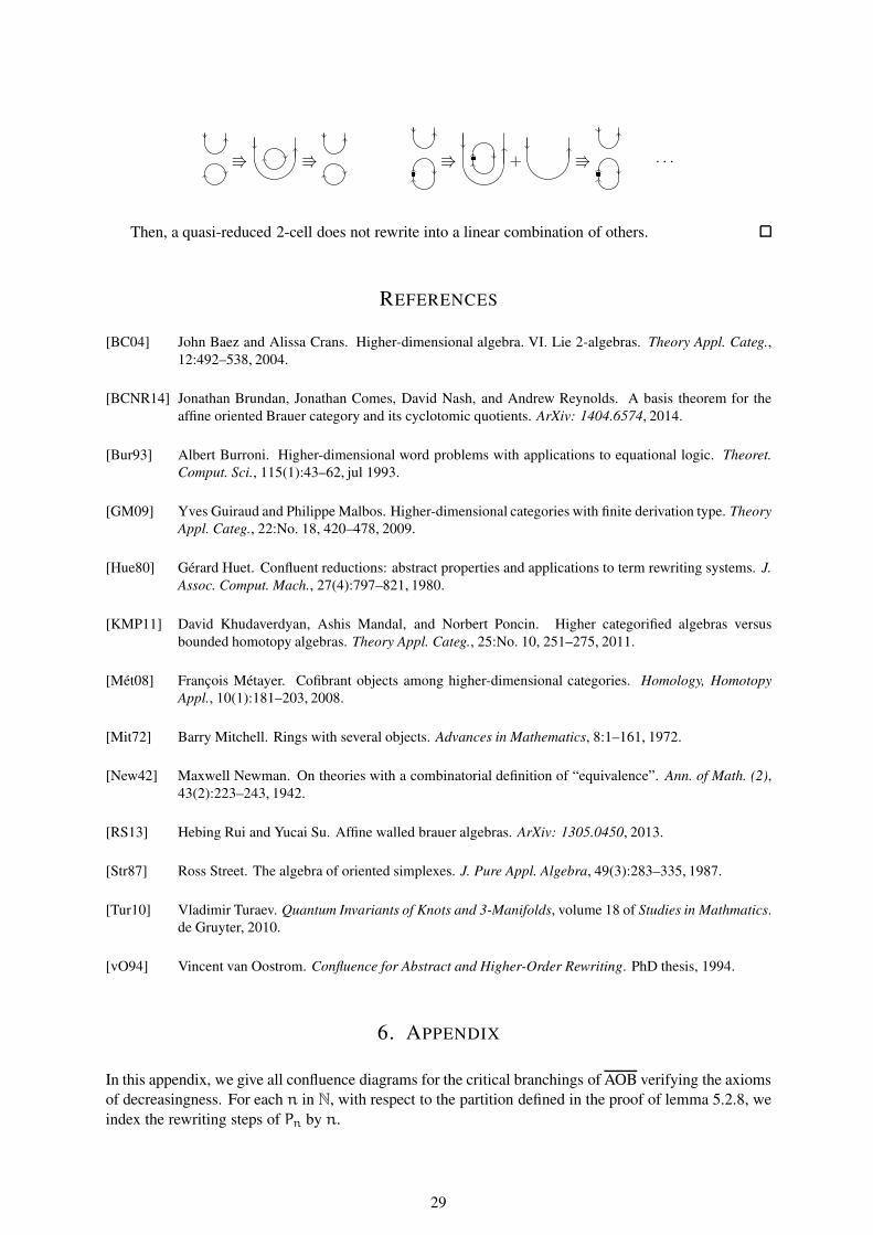
Then, a quasi-reduced 2-cell does not rewrite into a linear combination of others.

REFERENCES

[BC04] John Baez and Alissa Crans. Higher-dimensional algebra. VI. Lie 2-algebras. Theory Appl. Categ.,

12:492–538, 2004.

[BCNR14] Jonathan Brundan, Jonathan Comes, David Nash, and Andrew Reynolds. A basis theorem for the

affine oriented Brauer category and its cyclotomic quotients. ArXiv: 1404.6574, 2014.

[Bur93] Albert Burroni. Higher-dimensional word problems with applications to equational logic. Theoret.

Comput. Sci., 115(1):43–62, jul 1993.

[GM09] Yves Guiraud and Philippe Malbos. Higher-dimensional categories with finite derivation type. Theory

Appl. Categ., 22:No. 18, 420–478, 2009.

[Hue80] Gérard Huet. Confluent reductions: abstract properties and applications to term rewriting systems. J.

Assoc. Comput. Mach., 27(4):797–821, 1980.

[KMP11] David Khudaverdyan, Ashis Mandal, and Norbert Poncin. Higher categorified algebras versus

bounded homotopy algebras. Theory Appl. Categ., 25:No. 10, 251–275, 2011.

[Mét08] François Métayer. Cofibrant objects among higher-dimensional categories. Homology, Homotopy

Appl., 10(1):181–203, 2008.

[Mit72] Barry Mitchell. Rings with several objects. Advances in Mathematics, 8:1–161, 1972.

[New42] Maxwell Newman. On theories with a combinatorial definition of “equivalence”. Ann. of Math. (2),

43(2):223–243, 1942.

[RS13] Hebing Rui and Yucai Su. Affine walled brauer algebras. ArXiv: 1305.0450, 2013.

[Str87] Ross Street. The algebra of oriented simplexes. J. Pure Appl. Algebra, 49(3):283–335, 1987.

[Tur10] Vladimir Turaev. Quantum Invariants of Knots and 3-Manifolds, volume 18 of Studies in Mathmatics.

de Gruyter, 2010.

[vO94] Vincent van Oostrom. Confluence for Abstract and Higher-Order Rewriting. PhD thesis, 1994.

6. APPENDIX

In this appendix, we give all confluence diagrams for the critical branchings of AOB verifying the axioms

of decreasingness. For each n in N, with respect to the partition defined in the proof of lemma 5.2.8, we

index the rewriting steps of Pn by n.

29

⇚0 ⇛0

⇚0 ⇛2 ⇛1 ⇛0

⇚0 ⇚1 ⇚2 ⇛0

⇚0 ⇚1 ⇚2 ⇛0

⇛3 ⇛2 + ⇛1 + ⇛0 +

⇛2 ⇛1 + ⇛0 +

⇚0 ⇛2 ⇛1 ⇛0

⇚0 ⇛1 ⇛0 ⇚0 ⇛1 ⇛0

⇚0 ⇚1 + ⇚2 ⇛0

⇚0 ⇚1 ⇚2 ⇛2 ⇛1 ⇛0

30

⇚0 ⇚1 ⇚2 ⇛2 ⇛1 ⇛0

⇚0 ⇚1 ⇚2 ⇚3 ⇛2 ⇛1 ⇛0

⇚0 ⇚1 ⇚2 ⇛1 ⇛0

⇛3 + ⇛2 + + ⇛1 + + ⇛0 + +

⇛3 ⇛2 + ⇛1 + + ⇛0 + +

⇚0 ⇚1 ⇚2 ⇛2 ⇛1 ⇛0

⇚0 ⇚1 ⇚2 ⇛2 ⇛1 ⇛0

⇚0 ⇚1 ⇛1 ⇛0

31

⇚0 ⇚1 ⇚2 ⇚3 ⇛0

⇚0 ⇚1 ⇛2 ⇛1 ⇛0

⇚0 ⇚1 ⇛1 ⇛0

⇚0 ⇚1 ⇚2 ⇛0

+ ⇚0 + ⇚1 ⇛1 ⇛0 +

⇚0 ⇚1 ⇚2 ⇛2 ⇛1 ⇛0

⇚0 ⇚1 ⇚2 ⇛2 ⇛1 ⇛0

⇚0 ⇚1 ⇛1 ⇛0

32

⇛1 ⇛0

⇛5 + ⇛4 + ⇛3 − + ⇛2 − + ⇛1 ⇛0

⇚0 ⇚1 ⇚2 ⇛2 ⇛1 ⇛0

⇚0 ⇚1 + ⇚2 ⇛1 ⇛0

⇚0 ⇚1 ⇚2 ⇛0

⇚0 ⇚1 + ⇚2 + ⇚3 + ⇚4 ⇛0

⇚0 ⇚1 ⇚2 ⇛0

⇚0 + ⇚1 ⇛1 − ⇛0

⇚0 ⇛2 ⇛1 ⇛0

⇚0 ⇚1 ⇛1 ⇛0

33