Embed Size (px)
Citation preview

REVSTAT
STATISTICAL JOURNAL

Catalogação Recomendada
REVSTAT. Lisboa, 2003- Revstat : statistical journal / ed. Instituto Nacional de Estatística. - Vol. 1, 2003- . - Lisboa I.N.E., 2003- . - 30 cm Semestral. - Continuação de : Revista de Estatística = ISSN 0873-4275. - edição exclusivamente em inglês
ISSN 1645-6726
CREDITS
- EDITOR-IN-CHIEF - M. Ivette Gomes
- CO-EDITOR - M. Antónia Amaral Turkman
- ASSOCIATE EDITORS - Barry Arnold - Helena Bacelar- Nicolau - Susie Bayarri - João Branco - M. Lucília Carvalho - David Cox - Edwin Diday - Dani Gamerman - Marie Husková - Isaac Meilijson - M. Nazaré Mendes-Lopes - Stephan Morgenthaler - António Pacheco - Dinis Pestana - Ludger Rüschendorf - Gilbert Saporta - Jef Teugels
- EXECUTIVE EDITOR - Maria José Carrilho
- SECRETARY - Liliana Martins
- PUBLISHER - Instituto Nacional de Estatística, I.P. (INE, I.P.)
Av. António José de Almeida, 2 1000-043 LISBOA PORTUGAL Tel.: + 351 218 426 100 Fax: + 351 218 454 084 Web site: http://www.ine.pt Customer Support Service (National network): 808 201 808 (Other networks): + 351 218 440 695
- COVER DESIGN - Mário Bouçadas, designed on the stain glass
window at INE, I.P., by the painter Abel Manta
- LAYOUT AND GRAPHIC DESIGN - Carlos Perpétuo
- PRINTING - Instituto Nacional de Estatística, I.P.
- EDITION - 190 copies
- LEGAL DEPOSIT REGISTRATION - N.º 191915/03
PRICE
[VAT included]
- Single issue ……………………………………………………….. € 11 - Annual subscription (No. 1 Special Issue, No. 2 and No.3)………. € 26 - Annual subscription (No. 2, No. 3) ……………………………….. € 18
© INE, I.P., Lisbon. Portugal, 2013* Reproduction authorised except for commercial purposes by indicating the source.
INDEX
Nonparametric Estimation of the Tail-Dependence Coefficient
Marta Ferreira . . . . . . . . . . . . . . . . . . . . . . . . . . . . . . . . . . . . . . . . . . . . . . . . . . . . . . . 1
Noncentral Generalized Multivariate Beta Type II Distribution
K. Adamski, S.W. Human, A. Bekker and J.J.J. Roux . . . . . . . . . . . . . 17
Use of Survival Models in A Refinery
Sılvia Madeira, Paulo Infante and Filipe Didelet . . . . . . . . . . . . . . . . . . . . 45
Robust Methods in Acceptance Sampling
Elisabete Carolino and Isabel Barao . . . . . . . . . . . . . . . . . . . . . . . . . . . . . . . . 67
The Skew-Normal Distribution in SPC
Fernanda Figueiredo and M. Ivette Gomes . . . . . . . . . . . . . . . . . . . . . . . . . . 83
Improving SSA Predictions by Inverse Distance Weighting
Richard O. Awichi and Werner G. Muller . . . . . . . . . . . . . . . . . . . . . . . . . . 105
Abstracted/indexed in: Current Index to Statistics, DOAJ, Google Scholar, Journal CitationReports/Science Edition, Mathematical Reviews, Science Citation Index Expandedr, SCOPUSand Zentralblatt fur Mathematic.

REVSTAT – Statistical Journal
Volume 11, Number 1, March 2013, 1–16
NONPARAMETRIC ESTIMATION OF THE
TAIL-DEPENDENCE COEFFICIENT
Author: Marta Ferreira
– Center of Mathematics of Minho University, Portugal
Abstract:
• A common measure of tail dependence is the so-called tail-dependence coefficient.
We present a nonparametric estimator of the tail-dependence coefficient and prove
its strong consistency and asymptotic normality in the case of known marginal dis-
tribution functions. The finite-sample behavior as well as robustness will be assessed
through simulation. Although it has a good performance, it is sensitive to the extreme
value dependence assumption. We shall see that a block maxima procedure might im-
prove the estimation. This will be illustrated through simulation. An application to
financial data shall be presented at the end.
Key-Words:
• extreme value theory; stable tail dependence function; tail-dependence coefficient.
AMS Subject Classification:
• 62G32.

2 Marta Ferreira
TDC Estimation 3
1. INTRODUCTION
Modern risk management is highly interested in assessing the amount of tail
dependence. Many minimum-variance portfolio models are based on correlation,
but correlation itself is not enough to describe a tail dependence structure and
often results in misleading interpretations (Embrechts et al., [7]). Multivariate
extreme value theory (EVT) is the natural tool to measure and model such ex-
tremal dependence. The importance of this issue has led to several developments
and applications in literature, e.g., Sibuya ([25]), Tiago de Oliveira ([27]), Joe
([16]), Coles et al. ([5]), Embrechts et al. ([8]), Frahm et al. ([11]), Schmidt and
Stadtmuller ([23]), Ferreira and Ferreira ([9]); see de Carvalho and Ramos ([6])
for a recent survey.
The tail-dependence coefficient (TDC) measures the probability of occur-
ring extreme values for one random variable (r.v.) given that another assumes
an extreme value too. More precisely, it is defined as
λ = limt→∞
P(F1(X1) > 1 − 1/t | F2(X2) > 1 − 1/t
),(1.1)
where F1 and F2 are the distribution functions (d.f.’s) of r.v.’s X1 and X2, re-
spectively. Observe that it can be formulated as
λ = limα→0
P(X1 > VaR1−α(X1) | X2 > VaR1−α(X2)
),
where VaR1−α(Xi) (i = 1, 2) is the Value-at-Risk of Xi at probability level 1− α
given by the quantile function evaluated at 1 − α, F−1i (1 − α) = inf{x : Fi(x) ≥
1 − α} (see e.g., Schmidt and Stadtmuller, [23]). The TDC can also be defined
via the notion of copula, introduced by Sklar ([26]). A copula C is a cumulative
distribution function whose margins are uniformly distributed on [0, 1]. If C is
the copula of (X1, X2) having joint d.f. F , i.e., F (x1, x2) = C(F1(x1), F2(x2)
),
observe that
λ = 2 − limt→∞
tP(F1(X1) > 1 − 1/t or F2(X2) > 1 − 1/t
)
= 2 − limt→∞
t{
1 − C(1 − 1/t, 1 − 1/t
)}.
(1.2)
The TDC was the first tail dependence concept appearing in literature in a
Sibuya’s paper, where it was shown that, no matter how high we choose the
correlation of normal random pairs, if we go far enough into the tail, extreme
events tend to occur independently in each margin (Sibuya, [25]). It character-
izes the dependence in the tail of a random pair (X1, X2), in the sense that,
λ > 0 corresponds to tail dependence whose degree is measured by the value of λ,
whereas λ = 0 means tail independence. The well-known bivariate t-distribution
presents tail dependence, whereas the above mentioned bivariate normal is an
example of tail independent model.
4 Marta Ferreira
The conventional multivariate extreme value theory has emphasized the
asymptotically dependent class resulting in its wide use. However, if the series are
truly asymptotically independent, i.e., λ = 0, an overestimation of extreme value
dependence, and consequently of the risk, will take place (see, e.g., Poon et al.,
[21]; for further details about asymptotically independent class and respective
models and coefficients, see also Ledford and Tawn, [19, 20]). Therefore, it is
important to conclude whether (X1, X2) is tail dependent or not. In practice,
this is not an easy task and one must be careful by inferring tail dependence
from a finite random sample. Tests for tail independence can be seen in, e.g.,
Zhang ([28]), Husler and Li ([15]) and references therein. Frahm et al. ([11])
presents illustrations of misidentifications of the dependence structure. The bad
performance of several nonparametric TDC estimators under tail independence
was also shown in this latter paper through simulation. We remark that the
examples that were used only concern models whose dependence function is not
of the extreme value type. Here we present a nonparametric estimator for the
TDC derived from Ferreira and Ferreira ([10]) and thus under an extreme value
dependence, which we denote λ(FF). Strong consistency and asymptotic normality
are proved (this latter in the case of known marginal d.f.’s). The finite-sample
behavior and robustness are analyzed through simulation. We also compare with
other existing methods. The simulation studies reveal some sensitivity to an
extreme value dependence assumption and a large bias problem in the particular
case of tail independence. In practice this may be overcome by taking block
maxima, but one must be careful with a bias-variance trade-off arising from the
number of block maxima to be considered: the larger this number the smaller
the variance but the larger the bias (Frahm et al., [11]). The simulation studies
present improvements in estimates in some cases and allow to conclude the best
block length choice. We end with an application to financial data.
2. EVT AND TAIL DEPENDENCE
Let{(
X(n)1 , X
(n)2
)}n≥1
be i.i.d. copies of 2-dimensional random vector,
(X1, X2), with common d.f. F, and let M(n)j = max1≤i≤n X
(i)j , j = 1, 2, be the
partial maxima for each marginal. If there exist sequences of constants a(n)j > 0,
b(n)j ∈ R, for j = 1, 2, and a distribution function G with non-degenerate margins,
such that
P(M
(n)1 ≤ a
(n)1 x1 + b
(n)1 , M
(n)2 ≤ a
(n)2 x2 + b
(n)2
)=
= Fn(a
(n)1 x1 + b
(n)1 , a
(n)2 x2 + b
(n)2
)−→n→∞
G(x1, x2) ,(2.1)
TDC Estimation 5
for all continuity points of G(x1, x2), then it must be a bivariate extreme value
distribution, given by
(2.2) G(x1, x2) = exp
[−l{− log G1(x1), − log G2(x2)
}],
for some bivariate function l, where Gj , j = 1, 2, is the marginal d.f. of G.
We also say that F belongs to the max-domain of attraction of G, in short,
F ∈ D(G). The function l in (2.2) is called stable tail dependence function,
sometimes denoted extreme value dependence. It can be verified that l is con-
vex, is homogeneous of order 1, and that max(x1, x2) ≤ l(x1, x2) ≤ x1 + x2 for all
(x1, x2) ∈ [0,∞)2, where the upper bound is due to the positive dependence of
extreme value models and corresponds to independence whilst the lower bound
means complete dependence (see, e.g. Beirlant et al. [1], Section 8.2.2). These
properties also hold in the d-variate case, with d > 2. The statement in (2.1) has
a similar formulation for the respective copulas, say CX and C:
CnX(u
1/n1 , u
1/n2 ) −→
n→∞C(u1, u2) ,(2.3)
where
(2.4) C(u1, u2) = exp
{−l(− log u1, − log u2
)}
is called a bivariate extreme value copula. In the sequel it will be denoted BEV
copula and we will also refer the extreme value dependence context as a BEV
dependence. The defining feature of a BEV copula is the max-stability property,
i.e., C(u1, u2) = C(u1/m1 , u
1/m2 )
mfor every integer m ≥ 1, ∀ (u1, u2) ∈ [0, 1]
2. The
max-domain of attraction condition (2.1) implies (2.3) but the reciprocal is not
true since it must also be imposed that each marginal belongs to some max-
domain of attraction. Since we have
limt→∞
t P(F1(X1) > 1 − 1/t, F2(X2) > 1 − 1/t
)=
= 2 − limt→∞
t{
1 − C(1 − 1/t, 1 − 1/t
)}
= 2 − limt→∞
log Ct(1 − 1/t, 1 − 1/t
)
= 2 − limt→∞
log C((1 − 1/t)t, (1 − 1/t)t
)
= 2 − l(1, 1) ,
(2.5)
the TDC of a BEV copula can be obtained through the function l as
(2.6) λ = 2 − l(1, 1) .
In the following we list some examples of stable tail dependence functions
of BEV copulas and respective tail dependence:
• Logistic: l(v1, v2) = (v1/r1 + v
1/r2 )
r, with vj ≥ 0 and parameter 0 < r ≤ 1;
complete dependence is obtained in the limit as r → 0 and independence
when r = 1.
6 Marta Ferreira
• Asymmetric Logistic: l(v1, v2) = (1 − t1)v1 + (1 − t2)v2 +{(t1v1)
1/r+
(t2v2)1/r}r
, with vj ≥ 0 and parameters 0 < r≤ 1 and 0≤ tj ≤ 1, j = 1, 2;
when t1 = t2 = 1 the asymmetric logistic model is equivalent to the logis-
tic model; independence is obtained when either r = 1, t1 = 0 or t2 = 0.
Complete dependence is obtained in the limit when t1 = t2 = 1 and
r approaches zero.
• Husler–Reiss: l(v1, v2) = v1Φ(r−1
+12 r log(v1/v2)
)+ v2Φ
(r−1
+12 r ·
log(v2/v1)), with parameter r > 0 and where Φ is the standard nor-
mal d.f.; complete dependence is obtained as r → ∞ and independence
as r → 0.
Non-BEV copulas cannot be obtained in the limit in (2.3), i.e., do not
satisfy max-stability and cannot be expressed through formulation (2.4) based
on the extreme value dependence function l with the given properties.
Examples of non-BEV copulas correspond, for instance, to the class of
elliptical ones. The bivariate normal and the symmetric generalized hyperbolic
distributions are tail independent models within this class. On the other hand,
the bivariate t-distribution presents tail dependence with TDC,
λ = 2Ftν+1
{−√
(ν + 1) (1 − ρ)/(1 + ρ)
},
where ρ > −1 and Ftν+1 is the d.f. of the one dimensional tν+1 distribution. See,
e.g., Schmidt ([22]) and Frahm et al. ([11]).
Bivariate Archimedean copulas are another wide class that includes some
tail independent non-BEV copulas such as Clayton, C(u1,u2)=(u−θ1 +u−θ
2 −1)−1/θ
with θ ≥ 0. Another special type which do not belong to either one of the three
classes above is the tail independent Plackett-copula
C(u1, u2) =
1 + (θ−1)(u1+u2) −[{
1+(θ−1)(u1+u2)}2 − 4u1u2θ(θ−1)
]1/2
2 (θ−1),
with parameter θ ∈ R+\{1}, and C(u1, u2) = u1u2, if θ = 1. For more details,
see Joe ([16]).
3. ESTIMATION
The use of (semi)parametric estimators bears a model risk and may lead
to wrong interpretations of the dependence structure. Nonparametric procedures
avoid this type of misspecification but usually come along with a larger vari-
ance. Frahm et al. ([11]) confirms this assertion and shows that (semi)parametric
estimators may have disastrous performances under wrong model assumptions.
TDC Estimation 7
So, in practice, if we are not sure about the type of model underlying data,
nonparametric approach can be an alternative. Here we focus on nonparametric
methods.
Huang ([14]), considered an estimator derived from the definition in (1.2)
by plugging-in the respective empirical counterparts:
(3.1) λ(H)= 2 − 1
kn
n∑
i=1
1{ bF1(X(i)1 )>1− kn
nor bF2(X
(i)2 )>1− kn
n
} ,
where Fj is the empirical d.f. of Fj , j = 1, 2. Concerning estimation accuracy,
some modifications of this latter may be used, like replacing the denominator n
by n + 1, i.e., considering
Fj(u) =1
n + 1
n∑
i=1
1{X
(i)j ≤u
}
(Beirlant et al. [1], Section 9.4.1). A similar procedure was considered in Schimdt
and Stadtmuler ([23]). For asymptotic properties, see the more recent results in
Bucher and Dette ([2]). The consistency and asymptotic normality of the estima-
tor λ(H)are derived with the asymptotics holding for an intermediate sequence
{kn}, kn → ∞ and kn/n → 0, as n → ∞. The choice of k ≡ kn that allows for the
‘best’ bias–variance tradeoff is of major difficulty, since small values of k come
along with a large variance whenever an increasing k results in a strong bias. A
similar problem exists for univariate tail index estimations of heavy tailed dis-
tributions, for estimators of the stable tail dependence function l (Krajina, [18])
and other TDC estimators (e.g., Frahm et al. [11] and Schmidt and Stadtmuller
[23]).
Under a BEV copula assumption, i.e., a copula with formulation (2.4), and
given (2.6), estimators for the TDC can be obtained through the ones of the
stable tail dependence function l. Within this context and motivated in Caperaa
et al. ([4]), Frahm et al. ([11]) presented the estimator
2 − 2 exp
[1
n
n∑
i=1
log
(√log
1
F1(X(i)1 )
log1
F2(X(i)2 )
/log
1
max{F1(X
(i)1 ), F2(X
(i)2 )}2
)].
This rank-based estimator was shown to have the best performance among all
nonparametric estimators considered in Frahm et al. ([11]). Optimally corrected
versions can be seen in Genest and Segers ([12]) and alternative estimators are
presented in Bucher et al. ([3]). In the sequel, we shall use a corrected version
satisfying the boundary condition l(1, 0) = l(0, 1) = 1 considered in Genest and
Segers ([12]), and here denoted λ(CFG-C).
Our approach is motivated by Ferreira and Ferreira ([10]) and has the same
assumption of a BEV copula dependence structure. More precisely, it is based
8 Marta Ferreira
on the following representation of the stable tail dependence function:
(3.2) l(x1, x2) =
E[max
{F1(X1)
1/x1 , F2(X2)1/x2
}]
1 − E[max
{F1(X1)
1/x1 , F2(X2)1/x2
}] ,
where the expected values are estimated using sample means. Observe that the
d.f. of max(F1(X1)
1/x1 , F2(X2)1/x2
)is given by
P(max
{F1(X1)
1/x1 , F2(X2)1/x2
}≤ u
)= C
(ux1 , ux2
)
= exp
(−l(− log ux1 ,− log ux2
))
= exp
(−(− log u
)l(x1, x2
))
= ul(x1,x2) ,
(3.3)
where the penultimate step is due to the first order homogeneity property of
function l. Hence
E[max
{F1(X1)
1/x1 , F2(X2)1/x2
}]=
l(x1, x2)
1 + l(x1, x2).
Therefore, based on (2.6) and (3.2), we propose the estimator
λ(FF)= 3 −
[1− max
{F1(X1), F2(X2)
} ]−1,(3.4)
where max{F1(X1), F2(X2)
}is the sample mean of max
{F1(X1), F2(X2)
}, i.e.,
max{F1(X1), F2(X2)
}=
1
n
n∑
i=1
max{F1(X
(i)1 ), F2(X
(i)2 )}
.
Proposition 3.1. The estimator λ(FF) in (3.4) is strongly consistent.
Proof: Observe that
∣∣∣∣∣1
n
n∑
i=1
maxj∈{1,2}
{Fj
(X
(i)j
)}− E
[max
j∈{1,2}
{Fj
(Xj
)}]∣∣∣∣∣ ≤
≤∣∣∣∣∣1
n
n∑
i=1
maxj∈{1,2}
{Fj
(X
(i)j
)}− 1
n
n∑
i=1
maxj∈{1,2}
{Fj
(X
(i)j
)}∣∣∣∣∣
+
∣∣∣∣∣1
n
n∑
i=1
maxj∈{1,2}
{Fj
(X
(i)j
)}− E
[max
j∈{1,2}
{Fj
(Xj
)}]∣∣∣∣∣ ,
(3.5)
where the second term converges almost surely to zero by the Strong Law of
Large Numbers (by (3.3), maxj∈{1,2}
{Fj(Xj)
}∼ Beta
(l(1, 1), 1
), 1 ≤ l(1, 1) ≤ 2,
and all the moments exist).
TDC Estimation 9
The first term in (3.5) is upper bounded by
1
n
n∑
i=1
∑
j∈{1,2}
∣∣∣Fj
(X
(i)j
)− Fj
(X
(i)j
)∣∣∣ ,
which converges almost surely to zero according to Gilat and Hill ([13]; Theorem
1.1). See also Ferreira and Ferreira ([10], Proposition 3.7).
The asymptotic normality in case the marginal d.f.’s are known is derived
from Ferreira and Ferreira ([10], Proposition 3.3) and the delta method. More
precisely, denoting this version as λ(FF)∗ , we have
√n(λ
(FF)∗ −λ
)→ N(0, σ2
) ,
where
σ2=
l(1, 1)(1 + l(1, 1)
)2
2 + l(1, 1).
In the case of unknown marginals, we believe that the asymptotic normality of√n(λ(FF) −λ
)may be derived from the weak convergence of the empirical copula
process (Segers, [24]). This will be addressed in a future work.
Observe that estimators λ(FF)and λ(CFG-C)
are obtained under the more
restrictive assumption of an extreme value dependence but have a convergence
rate of√
n. On the other hand, estimator λ(H)has no restrictive assumptions
but has to pay the price of a slower convergence rate√
kn, since only the largest
kn = o(n) observations can be taken into account.
4. SIMULATION STUDY
In this section we analyze the finite-sample behavior of our estimator.
We simulate 1000 independent random samples of sizes n = 50, 100, 500, 1000
from three BEV copulas with stable tail dependence functions: logistic, asym-
metric logistic and Husler–Reiss. We consider the two types of dependence:
tail dependence (Table 1) and tail independence (Table 2). The results ob-
tained from the logistic and asymmetric logistic under tail independence are
quite similar and thus we omit the latter case. In order to assess robustness
we also analyze the case of non-BEV copulas, by considering, for tail depen-
dence, a bivariate t-distribution with ν = 1.5 degrees of freedom and, for tail
independence, a BSGH distribution (Table 3). In both cases we take a correla-
tion parameter of ρ = 0.5. Since the t-distribution is somewhat ‘close’ to being
an extreme value copula (see Bucher, Dette and Volgushev [3], Section 2), we
also consider a convex combination of a rotated Clayton copula (correspond-
ing to negative dependence) and a t-distribution, more precisely, Cα(u1, u2) =
α(u2 − CClayton(1 − u1, u2)
)+ (1 − α) Ctν (u1, u2). For comparison, we compute
estimator λ(CFG-C)which works under the same assumptions (i.e, an extreme
10 Marta Ferreira
value dependence) and the more general estimator λ(H)which has no model re-
strictions (the required choice of k to balance the variance-bias problem is based
on an heuristic procedure in Frahm et al. [11]). Absolute empirical bias and
the root mean-squared error (rmse) for all implemented TDC estimations are in
Tables 1, 2 and 3.
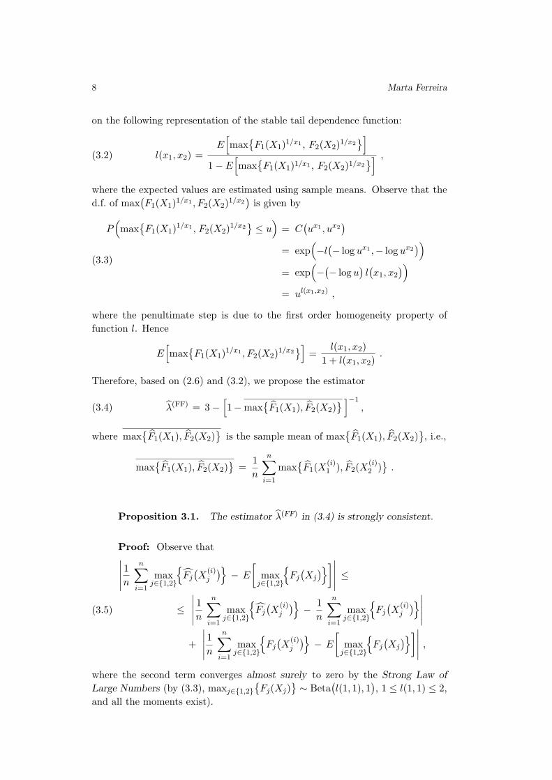
Table 1: Tail dependent (λ > 0) BEV copulas with stable tail depen-
dence functions: Logistic and Asym. Logistic with r = 0.4 and
Husler–Reiss with r = 3.
λ(FF) λ(CFG-C) λ(H)
bias (rmse) bias (rmse) bias (rmse)
λ = 0.6805 Logistic
(n = 50) 0.0019 (0.0994) 0.0050 (0.0556) 0.0395 (0.1962)
(n = 100) 0.0052 (0.0711) 0.0044 (0.0395) 0.0389 (0.1412)
(n = 500) 0.0006 (0.0330) 0.0005 (0.0180) 0.0216 (0.0883)
(n = 1000) 0.0002 (0.0232) 0.0004 (0.0122) 0.0099 (0.1379)
λ = 0.3402 Asym. Logistic
(n = 50) 0.0085 (0.1147) 0.0332 (0.1122) 0.0527 (0.1836)
(n = 100) 0.0053 (0.0824) 0.0203 (0.0754) 0.0635 (0.1363)
(n = 500) 0.0020 (0.0389) 0.0045 (0.0355) 0.0335 (0.0847)
(n = 1000) 0.0014 (0.0287) 0.0031 (0.0245) 0.0038 (0.1193)
λ = 0.7389 Husler–Reiss
(n = 50) 0.0040 (0.0484) 0.0057 (0.0462) 0.0202 (0.1697)
(n = 100) 0.0003 (0.0331) 0.0020 (0.0323) 0.0075 (0.1094)
(n = 500) 0.0002 (0.0152) 0.0007 (0.0140) 0.0011 (0.0655)
(n = 1000) 0.0002 (0.0292) 0.0005 (0.0097) 0.0103 (0.0342)
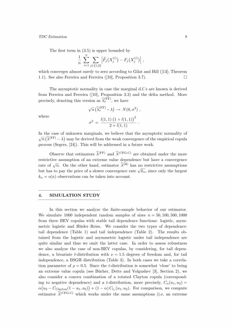
Table 2: Tail independent (λ = 0) BEV copulas with stable tail dependence
functions: Logistic with r = 1 and Husler–Reiss with r = 0.03.
λ(FF) λ(CFG-C) λ(H)
bias (rmse) bias (rmse) bias (rmse)
λ = 0 Logistic
(n = 50) 0.0230 (0.1284) 0.0900 (0.1389) 0.1040 (0.1644)
(n = 100) 0.0062 (0.0956) 0.0467 (0.0952) 0.1004 (0.1348)
(n = 500) 0.0036 (0.0415) 0.0140 (0.0361) 0.0492 (0.0650)
(n = 1000) 0.0017 (0.0296) 0.0077 (0.0257) 0.0502 (0.0578)
λ ≈ 0 Husler–Reiss
(n = 50) 0.0254 (0.1370) 0.0875 (0.1353) 0.1002 (0.1660)
(n = 100) 0.0084 (0.0966) 0.0412 (0.0883) 0.0991 (0.1336)
(n = 500) 0.0009 (0.0415) 0.0100 (0.0361) 0.0492 (0.0653)
(n = 1000) 0.0003 (0.0299) 0.0061 (0.0265) 0.0081 (0.0298)
TDC Estimation 11
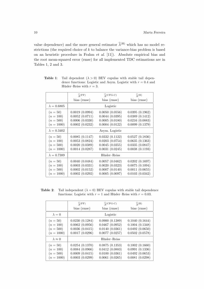
Table 3: Non-BEV tail dependent case: tν with ν = 1.5 and ρ = 0.5and a convex combination of a rotated Clayton and tν (RC&T),
C0.5(u1, u2) = 0.5(u2 − CClayton(1 − u1, u2)
)+ 0.5Ctν
(u1, u2);
non-BEV tail independent case: BSGH distribution with ρ = 0.5.
λ(FF) λ(CFG-C) λ(H)
bias (rmse) bias (rmse) bias (rmse)
λ = 0.4406 t-distribution
(n = 50) 0.0099 (0.1043) 0.0318 (0.1022) 0.0084 (0.1970)
(n = 100) 0.0087 (0.0711) 0.0213 (0.0743) 0.0094 (0.1393)
(n = 500) 0.0124 (0.0339) 0.0130 (0.0348) 0.0044 (0.0884)
(n = 1000) 0.0122 (0.0267) 0.0123 (0.0266) 0.0120 (0.1403)
λ = 0.3669 RC&T
(n = 50) 0.4396 (0.6562) 0.2832 (0.4736) 0.2990 (0.3064)
(n = 100) 0.4052 (0.6440) 0.2879 (0.4282) 0.1371 (0.2779)
(n = 500) 0.3800 (0.6411) 0.2793 (0.4681) 0.1350 (0.2772)
(n = 1000) 0.3791 (0.6342) 0.2650 (0.4571) 0.1314 (0.2743)
λ = 0 BSGH
(n = 50) 0.4288 (0.4396) 0.4305 (0.4544) 0.3730 (0.4238)
(n = 100) 0.4287 (0.4346) 0.4239 (0.4294) 0.3704 (0.3926)
(n = 500) 0.4248 (0.4259) 0.4030 (0.4052) 0.3130 (0.3232)
(n = 1000) 0.4238 (0.4243) 0.4001 (0.4008) 0.2188 (0.2489)
Estimators λ(FF)and λ(CFG-C)
behave well within BEV copulas (or ‘close’
of being BEV as t-distribution). Yet, they performed poorly on a non-BEV de-
pendence context (see Table 3). Estimator λ(H)tends to present a slight larger
bias but performs better under non extreme value dependence. This is consistent
with a slower rate of convergence and the fact that it holds in a general frame-
work, as discussed in the previous section. All estimators also performed poorly
on tail independent non-BEV copulas. Our results do not contradict however the
ones in Frahm et al. ([11]), where the misbehavior of nonparametric estimation
concerned tail independence within non-BEV copulas. By considering a block
maxima procedure, i.e., divide n-length data into m blocks of size b = ⌊n/m⌋(⌊x⌋ denotes the largest integer not exceeding x) and take only the maximum
observation within each block, we obtain a sample of maximum, which is more
consistent with an extreme values model and thus a BEV copula. This method-
ology involves a bias–variance tradeoff arising from the number of block maxima
(block length) to be considered: the larger (smaller) this number the smaller
the variance but the larger the bias (Frahm et al., [11]). It requires not too
small sample sizes to also provide not too small maxima samples. A simulation
study to find the value(s) of b that better accommodates this compromise will be
implemented in the next section.
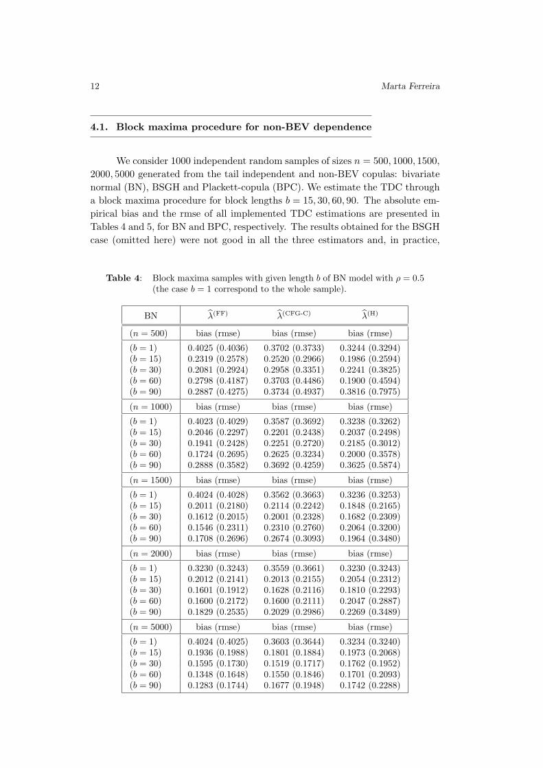
12 Marta Ferreira
4.1. Block maxima procedure for non-BEV dependence
We consider 1000 independent random samples of sizes n = 500, 1000, 1500,
2000, 5000 generated from the tail independent and non-BEV copulas: bivariate
normal (BN), BSGH and Plackett-copula (BPC). We estimate the TDC through
a block maxima procedure for block lengths b = 15, 30, 60, 90. The absolute em-
pirical bias and the rmse of all implemented TDC estimations are presented in
Tables 4 and 5, for BN and BPC, respectively. The results obtained for the BSGH
case (omitted here) were not good in all the three estimators and, in practice,
Table 4: Block maxima samples with given length b of BN model with ρ = 0.5(the case b = 1 correspond to the whole sample).
BN λ(FF) λ(CFG-C) λ(H)
(n = 500) bias (rmse) bias (rmse) bias (rmse)
(b = 1) 0.4025 (0.4036) 0.3702 (0.3733) 0.3244 (0.3294)
(b = 15) 0.2319 (0.2578) 0.2520 (0.2966) 0.1986 (0.2594)
(b = 30) 0.2081 (0.2924) 0.2958 (0.3351) 0.2241 (0.3825)
(b = 60) 0.2798 (0.4187) 0.3703 (0.4486) 0.1900 (0.4594)
(b = 90) 0.2887 (0.4275) 0.3734 (0.4937) 0.3816 (0.7975)
(n = 1000) bias (rmse) bias (rmse) bias (rmse)
(b = 1) 0.4023 (0.4029) 0.3587 (0.3692) 0.3238 (0.3262)
(b = 15) 0.2046 (0.2297) 0.2201 (0.2438) 0.2037 (0.2498)
(b = 30) 0.1941 (0.2428) 0.2251 (0.2720) 0.2185 (0.3012)
(b = 60) 0.1724 (0.2695) 0.2625 (0.3234) 0.2000 (0.3578)
(b = 90) 0.2888 (0.3582) 0.3692 (0.4259) 0.3625 (0.5874)
(n = 1500) bias (rmse) bias (rmse) bias (rmse)
(b = 1) 0.4024 (0.4028) 0.3562 (0.3663) 0.3236 (0.3253)
(b = 15) 0.2011 (0.2180) 0.2114 (0.2242) 0.1848 (0.2165)
(b = 30) 0.1612 (0.2015) 0.2001 (0.2328) 0.1682 (0.2309)
(b = 60) 0.1546 (0.2311) 0.2310 (0.2760) 0.2064 (0.3200)
(b = 90) 0.1708 (0.2696) 0.2674 (0.3093) 0.1964 (0.3480)
(n = 2000) bias (rmse) bias (rmse) bias (rmse)
(b = 1) 0.3230 (0.3243) 0.3559 (0.3661) 0.3230 (0.3243)
(b = 15) 0.2012 (0.2141) 0.2013 (0.2155) 0.2054 (0.2312)
(b = 30) 0.1601 (0.1912) 0.1628 (0.2116) 0.1810 (0.2293)
(b = 60) 0.1600 (0.2172) 0.1600 (0.2111) 0.2047 (0.2887)
(b = 90) 0.1829 (0.2535) 0.2029 (0.2986) 0.2269 (0.3489)
(n = 5000) bias (rmse) bias (rmse) bias (rmse)
(b = 1) 0.4024 (0.4025) 0.3603 (0.3644) 0.3234 (0.3240)
(b = 15) 0.1936 (0.1988) 0.1801 (0.1884) 0.1973 (0.2068)
(b = 30) 0.1595 (0.1730) 0.1519 (0.1717) 0.1762 (0.1952)
(b = 60) 0.1348 (0.1648) 0.1550 (0.1846) 0.1701 (0.2093)
(b = 90) 0.1283 (0.1744) 0.1677 (0.1948) 0.1742 (0.2288)
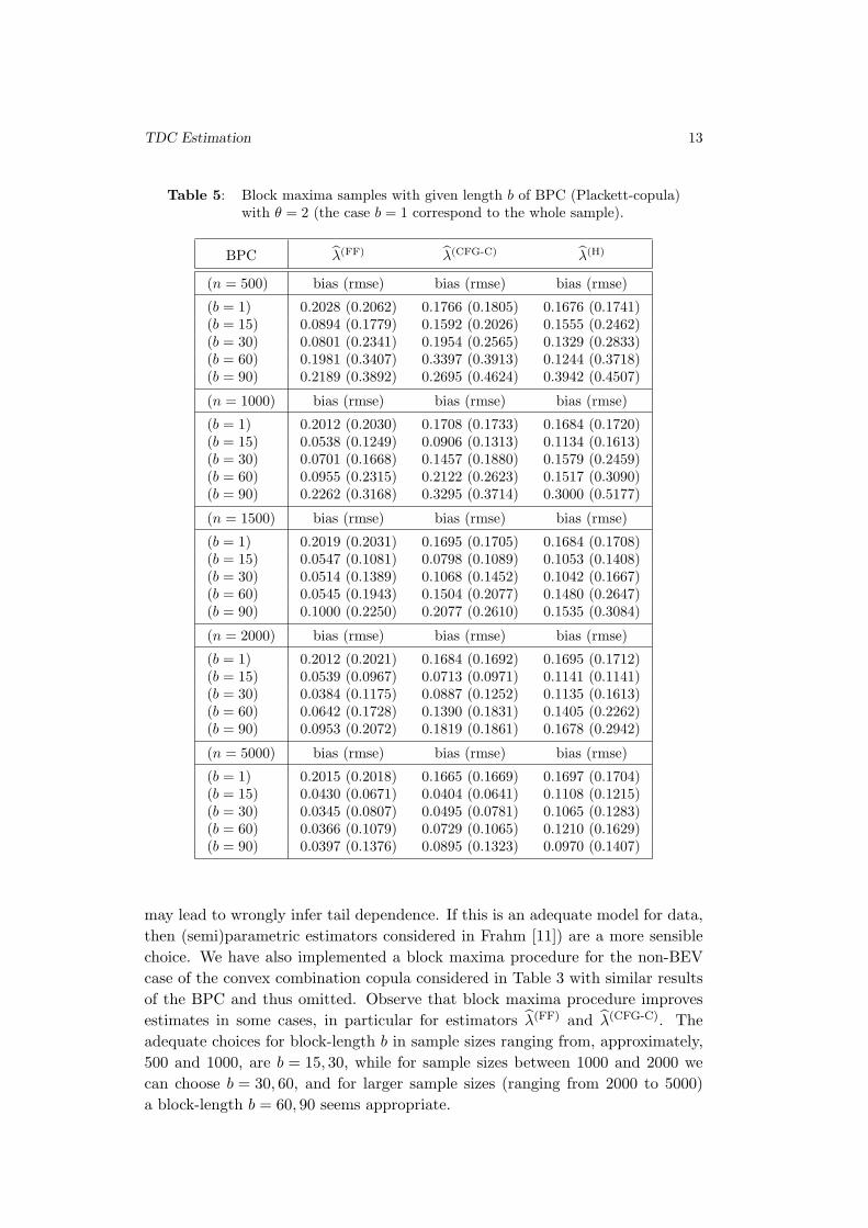
TDC Estimation 13
Table 5: Block maxima samples with given length b of BPC (Plackett-copula)
with θ = 2 (the case b = 1 correspond to the whole sample).
BPC λ(FF) λ(CFG-C) λ(H)
(n = 500) bias (rmse) bias (rmse) bias (rmse)
(b = 1) 0.2028 (0.2062) 0.1766 (0.1805) 0.1676 (0.1741)
(b = 15) 0.0894 (0.1779) 0.1592 (0.2026) 0.1555 (0.2462)
(b = 30) 0.0801 (0.2341) 0.1954 (0.2565) 0.1329 (0.2833)
(b = 60) 0.1981 (0.3407) 0.3397 (0.3913) 0.1244 (0.3718)
(b = 90) 0.2189 (0.3892) 0.2695 (0.4624) 0.3942 (0.4507)
(n = 1000) bias (rmse) bias (rmse) bias (rmse)
(b = 1) 0.2012 (0.2030) 0.1708 (0.1733) 0.1684 (0.1720)
(b = 15) 0.0538 (0.1249) 0.0906 (0.1313) 0.1134 (0.1613)
(b = 30) 0.0701 (0.1668) 0.1457 (0.1880) 0.1579 (0.2459)
(b = 60) 0.0955 (0.2315) 0.2122 (0.2623) 0.1517 (0.3090)
(b = 90) 0.2262 (0.3168) 0.3295 (0.3714) 0.3000 (0.5177)
(n = 1500) bias (rmse) bias (rmse) bias (rmse)
(b = 1) 0.2019 (0.2031) 0.1695 (0.1705) 0.1684 (0.1708)
(b = 15) 0.0547 (0.1081) 0.0798 (0.1089) 0.1053 (0.1408)
(b = 30) 0.0514 (0.1389) 0.1068 (0.1452) 0.1042 (0.1667)
(b = 60) 0.0545 (0.1943) 0.1504 (0.2077) 0.1480 (0.2647)
(b = 90) 0.1000 (0.2250) 0.2077 (0.2610) 0.1535 (0.3084)
(n = 2000) bias (rmse) bias (rmse) bias (rmse)
(b = 1) 0.2012 (0.2021) 0.1684 (0.1692) 0.1695 (0.1712)
(b = 15) 0.0539 (0.0967) 0.0713 (0.0971) 0.1141 (0.1141)
(b = 30) 0.0384 (0.1175) 0.0887 (0.1252) 0.1135 (0.1613)
(b = 60) 0.0642 (0.1728) 0.1390 (0.1831) 0.1405 (0.2262)
(b = 90) 0.0953 (0.2072) 0.1819 (0.1861) 0.1678 (0.2942)
(n = 5000) bias (rmse) bias (rmse) bias (rmse)
(b = 1) 0.2015 (0.2018) 0.1665 (0.1669) 0.1697 (0.1704)
(b = 15) 0.0430 (0.0671) 0.0404 (0.0641) 0.1108 (0.1215)
(b = 30) 0.0345 (0.0807) 0.0495 (0.0781) 0.1065 (0.1283)
(b = 60) 0.0366 (0.1079) 0.0729 (0.1065) 0.1210 (0.1629)
(b = 90) 0.0397 (0.1376) 0.0895 (0.1323) 0.0970 (0.1407)
may lead to wrongly infer tail dependence. If this is an adequate model for data,
then (semi)parametric estimators considered in Frahm [11]) are a more sensible
choice. We have also implemented a block maxima procedure for the non-BEV
case of the convex combination copula considered in Table 3 with similar results
of the BPC and thus omitted. Observe that block maxima procedure improves
estimates in some cases, in particular for estimators λ(FF)and λ(CFG-C)
. The
adequate choices for block-length b in sample sizes ranging from, approximately,
500 and 1000, are b = 15, 30, while for sample sizes between 1000 and 2000 we
can choose b = 30, 60, and for larger sample sizes (ranging from 2000 to 5000)
a block-length b = 60, 90 seems appropriate.
14 Marta Ferreira
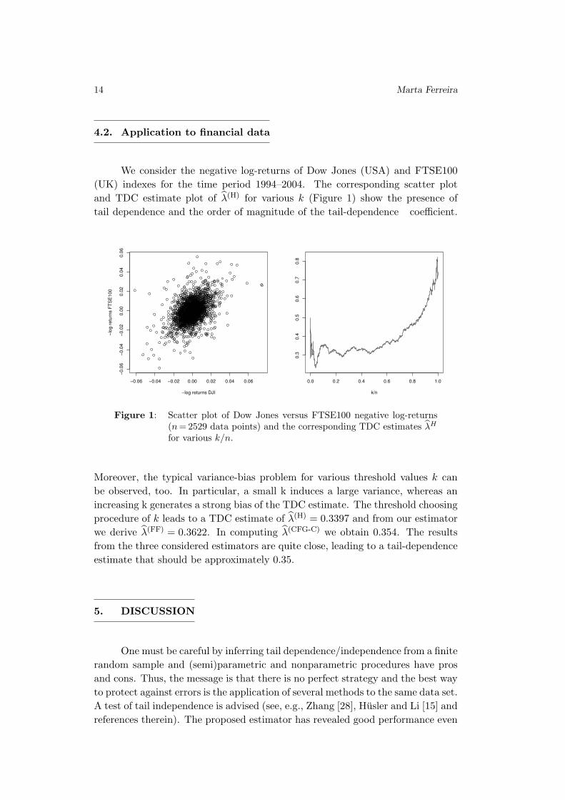
4.2. Application to financial data
We consider the negative log-returns of Dow Jones (USA) and FTSE100
(UK) indexes for the time period 1994–2004. The corresponding scatter plot
and TDC estimate plot of λ(H)for various k (Figure 1) show the presence of
tail dependence and the order of magnitude of the tail-dependence coefficient.
−0.06 −0.04 −0.02 0.00 0.02 0.04 0.06
−0.0
6−
0.0
4−
0.0
20.0
00.0
20.0
40.0
6
−log returns DJI
−lo
g r
etu
rns F
TS
E100
0.0 0.2 0.4 0.6 0.8 1.0
0.3
0.4
0.5
0.6
0.7
0.8
k/n
Figure 1: Scatter plot of Dow Jones versus FTSE100 negative log-returns
(n = 2529 data points) and the corresponding TDC estimates λH
for various k/n.
Moreover, the typical variance-bias problem for various threshold values k can
be observed, too. In particular, a small k induces a large variance, whereas an
increasing k generates a strong bias of the TDC estimate. The threshold choosing
procedure of k leads to a TDC estimate of λ(H)= 0.3397 and from our estimator
we derive λ(FF)= 0.3622. In computing λ(CFG-C)
we obtain 0.354. The results
from the three considered estimators are quite close, leading to a tail-dependence
estimate that should be approximately 0.35.
5. DISCUSSION
One must be careful by inferring tail dependence/independence from a finite
random sample and (semi)parametric and nonparametric procedures have pros
and cons. Thus, the message is that there is no perfect strategy and the best way
to protect against errors is the application of several methods to the same data set.
A test of tail independence is advised (see, e.g., Zhang [28], Husler and Li [15] and
references therein). The proposed estimator has revealed good performance even
TDC Estimation 15
in the independent case. However the simulation results showed sensitivity to the
assumption of an extreme value dependence structure and we recommend to test
in advance for this hypothesis. See Kojadinovic, Yan and Segers ([17]) or Bucher,
Dette and Volgushev ([3]) and references therein. A block maxima procedure
may improve the estimates. A study focused on the asymptotic properties will
be addressed in a future work.
ACKNOWLEDGMENTS
This research was financed by FEDER Funds through “Programa Opera-
cional Factores de Competitividade — COMPETE” and by Portuguese Funds
through FCT — “Fundacao para a Ciencia e a Tecnologia”, within the Project
Est-C/MAT/UI0013/2011.
We also acknowledge the valuable suggestions from the referees.
REFERENCES
[1] Beirlant, J.; Goegebeur, Y.; Segers, J. and Teugels, J. (2004). Statistics
Of Extremes: Theory and Application, John Wiley, England.
[2] Bucher, A. and Dette, H. (2012). Multiplier bootstrap of tail copulas with
applications, Bernoulli, to appear.
[3] Bucher, A.; Dette, H. and Volgushev, S. (2011). New estimators of the
Pickands dependence function and a test for extreme-value dependence, The An-
nals of Statistics, 39(4), 1963–2006.
[4] Caperaa, P.; Fougeres, A.L. and Genest, C. (1997). A nonparametric
estimation procedure for bivariate extreme value copulas, Biometrika, 84,
567–577.
[5] Coles, S.; Heffernan, J. and Tawn, J. (1999). Dependence measures for
extreme value analysis, Extremes, 2, 339–366.
[6] de Carvalho, M. and Ramos, A. (2012). Bivariate extreme statistics, II,
Revstat, 10, 83–107.
[7] Embrechts, P.; McNeil, A. and Straumann, D. (2002). Correlation and
dependence in risk management: properties and pitfalls. In “Risk Management:
Value at Risk and Beyond”(M.A.H. Dempster, Ed.), Cambridge University Press,
Cambridge, 176–223.
[8] Embrechts, P.; Lindskog, F. and McNeil, A. (2003). Modelling dependence
with copulas and applications to risk management. In “Handbook of Heavy Tailed
Distributions in Finance” (S. Rachev, Ed.), Elsevier, 329–384.
16 Marta Ferreira
[9] Ferreira, H. and Ferreira, M. (2012). Tail dependence between order statis-
tics, Journal of Multivariate Analysis, 105(1), 176–192.
[10] Ferreira, H. and Ferreira, M. (2012). On extremal dependence of block
vectors, Kybernetika, 48(5), 988–1006.
[11] Frahm, G.; Junker, M. and Schmidt, R. (2005). Estimating the tail-
dependence coefficient: properties and pitfalls, Insurance: Mathematics & Eco-
nomics, 37(1), 80–100.
[12] Genest, C. and Segers, J. (2009). Rank-based inference for bivariate extreme-
value copulas, The Annals of Statistics, 37, 2990–3022.
[13] Gilat, D. and Hill, T. (1992). One-sided refinements of the strong law of
large numbers and the Glivenko–Cantelli Theorem, The Annals of Probability,
20, 1213–1221.
[14] Huang, X. (1992). Statistics of Bivariate Extreme Values, Ph. D. thesis, Tin-
bergen Institute Research Series 22, Erasmus University, Rotterdam.
[15] Husler, J. and Li, D. (2009). Testing asymptotic independence in bivariate
extremes, Journal of Statistical Planning and Inference, 139, 990–998.
[16] Joe, H. (1997). Multivariate Models and Dependence Concepts, Chapman &
Hall, London.
[17] Kojadinovic, I.; Segers, J. and Yan, J. (2011). Large-sample tests of
extreme-value dependence for multivariate copulas, The Canadian Journal of
Statistics, 39(4), 703–720.
[18] Krajina, A. (2010). An M–Estimator of Multivariate Tail Dependence, Tilburg
University Press, Tilburg.
[19] Ledford, A. and Tawn, J.A. (1996). Statistics for near independence in mul-
tivariate extreme values, Biometrika, 83, 169–187.
[20] Ledford, A. and Tawn, J.A. (1997). Modelling dependence within joint tail
regions, Journal of the Royal Statistical Society, Series B, 59, 475–499.
[21] Poon, S.-H.; Rockinger, M. and Tawn, J. (2004). Extreme value dependence
in financial markets: diagnostics, models, and financial implications, Review of
Financial Studies, 17(2), 581–610.
[22] Schmidt, R. (2002). Tail dependence for elliptically contoured distributions,
Mathematical Methods of Operations Research, 55, 301–327.
[23] Schmidt, R. and Stadtmuller, U. (2006). Nonparametric estimation of tail
dependence, Scandinavian Journal of Statistics, 33, 307–335.
[24] Segers, J. (2012). Asymptotics of empirical copula processes under nonrestric-
tive smoothness assumptions, Bernoulli, 18, 764–782.
[25] Sibuya, M. (1960). Bivariate extreme statistics, Annals of the Institute of Sta-
tistical Mathematics, 11, 195–210.
[26] Sklar, A. (1959). Fonctions de repartition a n dimensions et leurs marges,
Publications de l’Institut de Statistique de l’Universite de Paris, 8, 229–231.
[27] Tiago de Oliveira, J. (1962–1963). Structure theory of bivariate extremes:
extensions, Estudos de Matematica, Estatıstica e Econometria, 7, 165–195.
[28] Zhang, Z. (2008). Quotient correlation: a sample based alternative to Pearson’s
correlation, The Annals of Statistics, 36(2), 1007–1030.
REVSTAT – Statistical Journal
Volume 11, Number 1, March 2013, 17–43
NONCENTRAL GENERALIZED MULTIVARIATE
BETA TYPE II DISTRIBUTION
Authors: K. Adamski, S.W. Human, A. Bekker and J.J.J. Roux
– University of Pretoria, Pretoria, 0002, South Africa
Abstract:
• The distribution of the variables that originates from monitoring the variance when
the mean encountered a sustained shift is considered — specifically for the case when
measurements from each sample are independent and identically distributed normal
random variables. It is shown that the solution to this problem involves a sequence
of dependent random variables that are constructed from independent noncentral chi-
squared random variables. This sequence of dependent random variables are the key
to understanding the performance of the process used to monitor the variance and
are the focus of this article. For simplicity, the marginal (i.e. the univariate and
bivariate) distributions and the joint (i.e. the trivariate) distribution of only the first
three random variables following a change in the variance is considered. A multivariate
generalization is proposed which can be used to calculate the entire run-length (i.e.
the waiting time until the first signal) distribution.
Key-Words:
• confluent hypergeometric functions; hypergeometric functions; multivariate beta dis-
tribution; noncentral chi-squared; shift in process mean and variance.
AMS Subject Classification:
• 62E15, 62H10.

18 Adamski, Human, Bekker and Roux
Noncentral Generalized Multivariate Beta 19
1. INTRODUCTION
We propose a noncentral generalized multivariate beta type II distribution
constructed from independent noncentral chi-squared random variables using the
variables in common technique. This is a new contribution to the existing beta
type II distributions considered in the literature. Tang (1938) studied the dis-
tribution of the ratios of noncentral chi-squared random variables defined on the
positive domain. He considered the ratio, consisting of independent variates,
where the numerator was a noncentral chi-squared random variable while the de-
nominator was a central chi-squared random variable, as well as the ratio where
both the numerator and denominator were noncentral chi-squared random vari-
ables — this was applied to study the properties of analysis of variance tests
under nonstandard conditions. Patnaik (1949) coined the phrase noncentral F
for the first ratio mentioned above. The second ratio is referred to as the doubly
noncentral F distribution. An overview of these distributions is given by John-
son, Kotz & Balakrishnan (1995). More recently Pe and Drygas (2006) proposed
an alternative presentation for the doubly noncentral F by using the results on
the product of two hypergeometric functions. In a bivariate context Gupta et al.
(2009) derived a noncentral bivariate beta type I distribution, using a ratio of
noncentral gamma random variables, that is defined on the unit square; applying
the appropriate transformation will yield a noncentral beta type II distribution
defined on the positive domain. The noncentral Dirichlet type II distribution
was derived by Troskie (1967) as the joint distribution of Vi =Yi
Yr+1, i = 1, 2, ..., r
where Yi is chi-squared distributed and Yr+1 has a noncentral chi-squared distri-
bution. Sanchez and Nagar (2003) derived the version where both Yi and Yr+1
are noncentral gamma random variables.
Section 2 provides an overview of the practical problem which is the gene-
sis of the random variables U0 =λW0X and Uj =
λWj
X +λ∑j−1
k=0Wk
, j = 1, 2, ..., p with
λ > 0 where X and Wi, i = 0, 1, ..., p are noncentral chi-squared distributed.
In Section 3 the distribution of the first three random variables, i.e. U0, U1, U2 is
derived. Bivariate densities and univariate densities of (U0, U1, U2) also receive at-
tention. Section 4 proposes a multivariate extension, followed by shape analysis,
an example and probability calculations in Sections 5 and 6, respectively.
2. PROBLEM STATEMENT
Adamski et al. (2012) proposed a generalized multivariate beta distribution;
the dependence structure and construction of the random variables originate in
a practical setting where the process mean is monitored, using a control chart
20 Adamski, Human, Bekker and Roux
(see e.g. Montgomery, 2009), when the measurements are independent and iden-
tically distributed having been collected from an Exp(θ) distribution, where θ
was assumed to be unknown.
Monitoring the unknown process variance assuming that the observations
from each independent sample are independent identically distributed (i.i.d.) nor-
mal random variables with the mean known was introduced by Quesenberry
(1991). To gain insight into the performance of such a control chart, in other
words, to determine the probability of detecting a shift immediately or after a
number of samples, the joint distribution of the plotting statistics is needed.
Exact expressions for the joint distribution of the plotting statistics for the chart
proposed by Quesenberry (1991) can be obtained from the distribution derived
by Adamski et al. (2012), the key difference is the fact that it is only the degrees
of freedom of the chi-squared random variables that changes.
Monitoring of the unknown process variance when the known location pa-
rameter sustained a permanent shift leads to a noncentral version of the gen-
eralized multivariate beta distribution proposed by Adamski et al. (2012). To
derive this new noncentral generalized multivariate beta type II distribution we
proceed in two steps. First we describe the practical setting which motivates
the derivation of the distribution, and secondly we derive the distributions in
sections 3 and 4. To this end, let (Xi1, Xi2, ..., Xini), i = 1, 2, ... represent suc-
cessive, independent samples of size ni ≥ 1 measurements made on a sequence of
items produced in time. Assume that these values are independent and identi-
cally distributed having been collected from a N(µ0, σ2) distribution where the
parameters µ0 and σ2denotes the known process mean and unknown process
variance, respectively. Take note that a sample can even consist of an individual
observation because the process mean is assumed to be known and the variance of
the sample can still be calculated as S2i = (Xi1 −µ0)
2. Suppose that from sample
(time period) κ > 1 the unknown process variance parameter has changed from
σ2to σ2
1 = λσ2(also unknown) where λ 6= 1 and λ > 0, but the known process
mean also encountered an unknown sustained shift from sample (time period)
h > 1 onwards, i.e. it changed from µ0 to µ1 where µ1 is also known. To clarify,
the mean of the process at start-up is assumed to be known and denoted µ0 but
the time and the size of the shift in the mean will be unknown in a practical
situation. In order to incorporate and/or evaluate the influence of these changes
in the parameters on the performance of the control chart for the variance, we
assume fixed/deterministic values for these parameters — essentially this implies
then that the mean is known following the shift, i.e. denoted by µ1. Therefore,
the main interest is monitoring the process variance when the process mean is
known, although this mean can suffer at some time an unknown shift. In prac-
tice it is important to note that even though the mean and the variance of the
normal distribution can change independently, the performance of a Shewhart
type control chart for the mean depends on the process variance and vice versa.
Noncentral Generalized Multivariate Beta 21
This dependency is due to the plotting statistics and the control limits used. The
proposed control chart could thus be useful in practice when the control chart
for monitoring the mean fails to detect the shift in the mean. For example, in
case a small shift in the mean occurs and a Shewhart-type chart for the mean is
used (which is known for the inefficiency in detecting small shifts compared to
the EWMA (exponentially weighted moving average) and CUSUM (cumulative
sum) charts for the mean which are better in detecting small shifts (Montgomery,
2009)) the shift might go undetected.
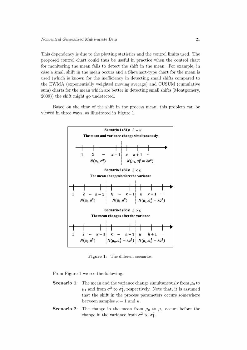
Based on the time of the shift in the process mean, this problem can be
viewed in three ways, as illustrated in Figure 1.
Figure 1: The different scenarios.
From Figure 1 we see the following:
Scenario 1: The mean and the variance change simultaneously from µ0 to
µ1 and from σ2to σ2
1, respectively. Note that, it is assumed
that the shift in the process parameters occurs somewhere
between samples κ − 1 and κ.
Scenario 2: The change in the mean from µ0 to µ1 occurs before the
change in the variance from σ2to σ2
1.
22 Adamski, Human, Bekker and Roux
Scenario 3: The change in the variance from σ2to σ2
1 occurs before the
change in the mean from µ0 to µ1.
Because it is assumed that the process variance σ2is unknown, the first
sample is used to obtain an initial estimate of σ2. Thus, in the remainder of
this article σ2is assumed to denote a point estimate of the unknown variance.
This initial estimate is continuously updated using the new incoming samples as
they are collected as long as the estimated value of σ2does not change, i.e. is
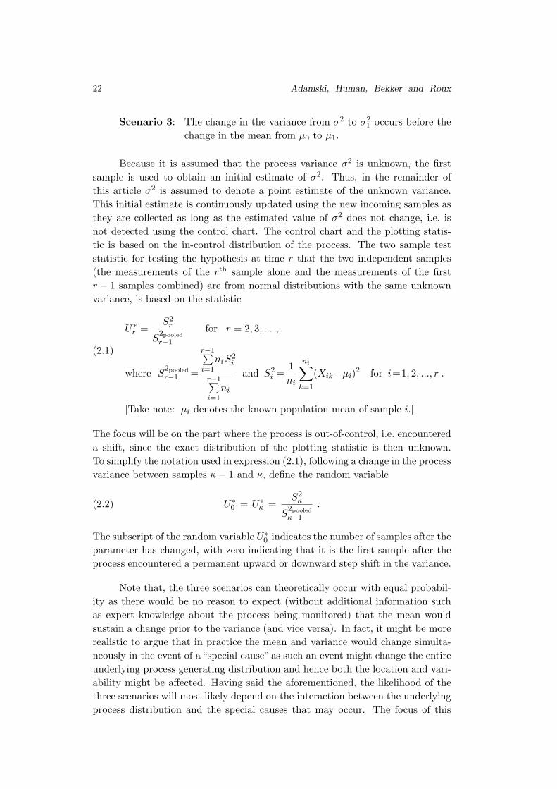
not detected using the control chart. The control chart and the plotting statis-
tic is based on the in-control distribution of the process. The two sample test
statistic for testing the hypothesis at time r that the two independent samples
(the measurements of the rthsample alone and the measurements of the first
r − 1 samples combined) are from normal distributions with the same unknown
variance, is based on the statistic
U∗r =
S2r
S2pooled
r−1
for r = 2, 3, ... ,
(2.1)
where S2pooled
r−1 =
r−1∑i=1
niS2i
r−1∑i=1
ni
and S2i =
1
ni
ni∑
k=1
(Xik−µi)2
for i=1, 2, ..., r .
[Take note: µi denotes the known population mean of sample i.]
The focus will be on the part where the process is out-of-control, i.e. encountered
a shift, since the exact distribution of the plotting statistic is then unknown.
To simplify the notation used in expression (2.1), following a change in the process
variance between samples κ − 1 and κ, define the random variable
(2.2) U∗0 = U∗
κ =S2
κ
S2pooled
κ−1
.
The subscript of the random variable U∗0 indicates the number of samples after the
parameter has changed, with zero indicating that it is the first sample after the
process encountered a permanent upward or downward step shift in the variance.
Note that, the three scenarios can theoretically occur with equal probabil-
ity as there would be no reason to expect (without additional information such
as expert knowledge about the process being monitored) that the mean would
sustain a change prior to the variance (and vice versa). In fact, it might be more
realistic to argue that in practice the mean and variance would change simulta-
neously in the event of a “special cause” as such an event might change the entire
underlying process generating distribution and hence both the location and vari-
ability might be affected. Having said the aforementioned, the likelihood of the
three scenarios will most likely depend on the interaction between the underlying
process distribution and the special causes that may occur. The focus of this
Noncentral Generalized Multivariate Beta 23
article is on scenario 2 since the results for the other scenarios follow by means
of simplifications (by setting the noncentrality parameter equal to zero) and will
be shown as remarks.
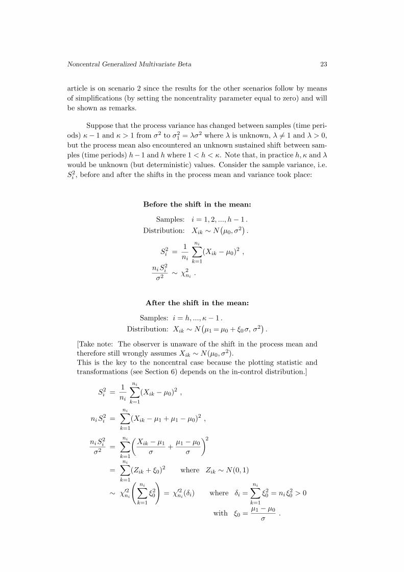
Suppose that the process variance has changed between samples (time peri-
ods) κ− 1 and κ > 1 from σ2to σ2
1 = λσ2where λ is unknown, λ 6= 1 and λ > 0,
but the process mean also encountered an unknown sustained shift between sam-
ples (time periods) h−1 and h where 1 < h < κ. Note that, in practice h, κ and λ
would be unknown (but deterministic) values. Consider the sample variance, i.e.
S2i , before and after the shifts in the process mean and variance took place:
Before the shift in the mean:
Samples: i = 1, 2, ..., h − 1 .
Distribution: Xik ∼ N(µ0, σ
2).
S2i =
1
ni
ni∑
k=1
(Xik − µ0)2 ,
niS2i
σ2∼ χ2
ni.
After the shift in the mean:
Samples: i = h, ..., κ − 1 .
Distribution: Xik ∼ N(µ1 = µ0 + ξ0σ, σ2
).
[Take note: The observer is unaware of the shift in the process mean and
therefore still wrongly assumes Xik ∼ N(µ0, σ2).
This is the key to the noncentral case because the plotting statistic and
transformations (see Section 6) depends on the in-control distribution.]
S2i =
1
ni
ni∑
k=1
(Xik − µ0)2 ,
niS2i =
ni∑
k=1
(Xik − µ1 + µ1 − µ0)2 ,
niS2i
σ2=
ni∑
k=1
(Xik − µ1
σ+
µ1 − µ0
σ
)2
=
ni∑
k=1
(Zik + ξ0)2
where Zik ∼ N(0, 1)
∼ χ′2ni
(ni∑
k=1
ξ20
)= χ′2
ni(δi) where δi =
ni∑
k=1
ξ20 = ni ξ
20 > 0
with ξ0 =µ1 − µ0
σ.

24 Adamski, Human, Bekker and Roux
After the shift in the mean and variance:
Samples: i = κ, κ + 1, ... .
Distribution: Xik ∼ N(µ1 = µ0 + ξ1σ1, σ2
1 = λσ2).
[Take note: The observer is unaware of the shifts in the process parameters
and therefore still wrongly assumes Xik ∼ N(µ0, σ2).]
S2i =
1
ni
ni∑
k=1
(Xik − µ0)2 ,
niS2i =
ni∑
k=1
(Xik − µ1 + µ1 − µ0)2 ,
niS2i
σ21
=
ni∑
k=1
(Xik − µ1
σ1+
µ1 − µ0
σ1
)2
=
ni∑
k=1
(Zik + ξ1)2
where Zik ∼ N(0, 1)
∼ χ′2ni
(ni∑
k=1
ξ21
)= χ′2
ni(δi) where δi =
ni∑
k=1
ξ21 = ni ξ
21 > 0
with ξ1 =µ1 − µ0
σ1.
Remark 2.1.
(i) χ2ni
denotes a central χ2random variable with degrees of freedom ni
(see Johnson et al. (1995), Chapter 18).
(ii) χ′2ni
(δi) denotes a noncentral χ2random variable with degrees of free-
dom ni and noncentrality parameter δi (see Johnson et al. (1995),
Chapter 29).
(iii) The degrees of freedom is assumed to be ni, since the mean is not es-
timated because it is assumed that the mean is a fixed / deterministic
value before and after the shift. In case the mean is unknown and
has to be estimated too, the degrees of freedom changes from ni to
ni − 1 and the µ0 would be replaced by µ0, i.e. an estimate of µ0.
(iv) The shift in the mean, before the variance changed, is modelled as
follows: ξ0 =µ1−µ0
σ , i.e. µ1 = µ0 + ξ0σ.
(v) The shift in the mean, after the variance changed, is modelled as
follows: ξ1 =µ1−µ0
σ1, i.e. µ1 = µ0 + ξ1σ1.
(vi) The pivotal quantityniS
2i
σ21
∼ χ′2ni
(δi) after the shift in the variance
reduces to a central chi-squared random variable if the process mean
did not change, i.e. when µ1 = µ0 (see Adamski et al. (2012)).
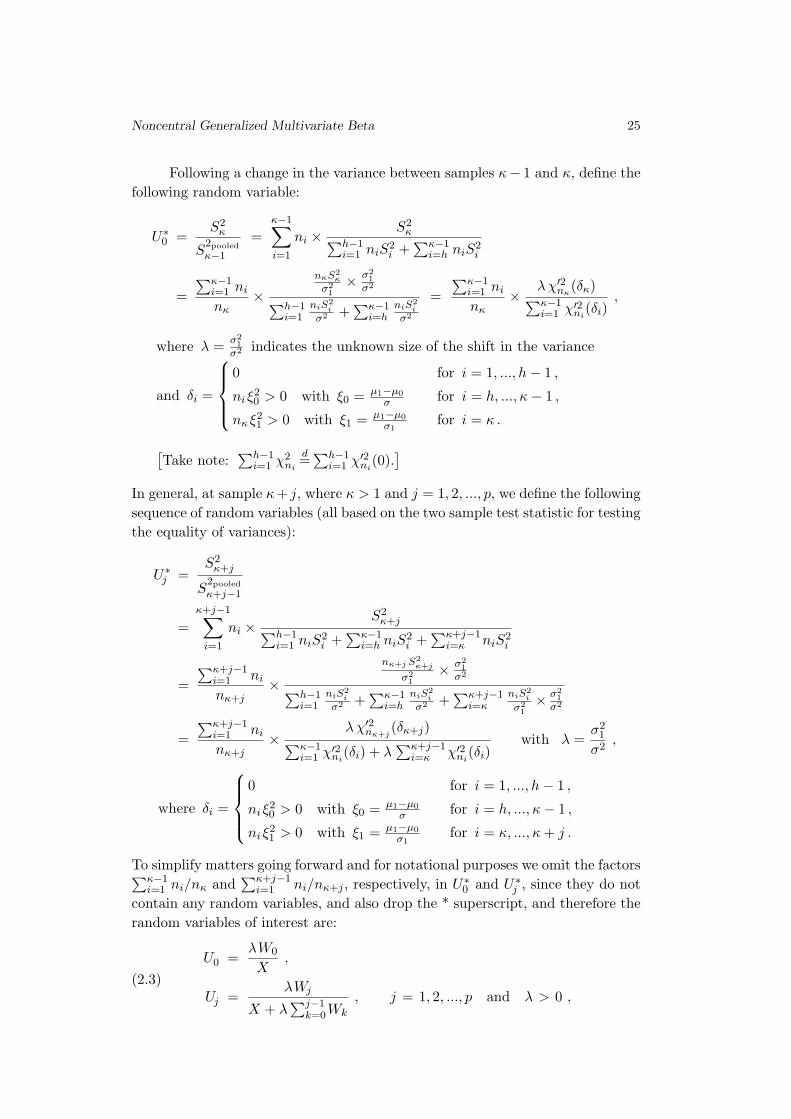
Noncentral Generalized Multivariate Beta 25
Following a change in the variance between samples κ− 1 and κ, define the
following random variable:
U∗0 =
S2κ
S2pooled
κ−1
=
κ−1∑
i=1
ni ×S2
κ∑h−1i=1 niS2
i +∑κ−1
i=h niS2i
=
∑κ−1i=1 ni
nκ×
nκS2κ
σ21
× σ21
σ2
∑h−1i=1
niS2i
σ2 +∑κ−1
i=hniS2
i
σ2
=
∑κ−1i=1 ni
nκ× λχ′2
nκ(δκ)
∑κ−1i=1 χ′2
ni(δi)
,
where λ =σ21
σ2 indicates the unknown size of the shift in the variance
and δi =
0 for i = 1, ..., h − 1 ,
ni ξ20 > 0 with ξ0 =
µ1−µ0
σ for i = h, ..., κ − 1 ,
nκ ξ21 > 0 with ξ1 =
µ1−µ0
σ1for i = κ .
[Take note:
∑h−1i=1 χ2
ni
d=∑h−1
i=1 χ′2ni
(0).]
In general, at sample κ+ j, where κ > 1 and j = 1, 2, ..., p, we define the following
sequence of random variables (all based on the two sample test statistic for testing
the equality of variances):
U∗j =
S2κ+j
S2pooled
κ+j−1
=
κ+j−1∑
i=1
ni ×S2
κ+j∑h−1i=1 niS2
i +∑κ−1
i=h niS2i +
∑κ+j−1i=κ niS2
i
=
∑κ+j−1i=1 ni
nκ+j×
nκ+j S2κ+j
σ21
× σ21
σ2
∑h−1i=1
niS2i
σ2 +∑κ−1
i=hniS2
i
σ2 +∑κ+j−1
i=κniS2
i
σ21
× σ21
σ2
=
∑κ+j−1i=1 ni
nκ+j×
λχ′2nκ+j
(δκ+j)
∑κ−1i=1 χ′2
ni(δi) + λ
∑κ+j−1i=κ χ′2
ni(δi)
with λ =σ2
1
σ2,
where δi =
0 for i = 1, ..., h − 1 ,
ni ξ20 > 0 with ξ0 =
µ1−µ0
σ for i = h, ..., κ − 1 ,
ni ξ21 > 0 with ξ1 =
µ1−µ0
σ1for i = κ, ..., κ + j .
To simplify matters going forward and for notational purposes we omit the factors∑κ−1i=1 ni/nκ and
∑κ+j−1i=1 ni/nκ+j , respectively, in U∗
0 and U∗j , since they do not
contain any random variables, and also drop the * superscript, and therefore the
random variables of interest are:
(2.3)
U0 =λW0
X,
Uj =λWj
X + λ∑j−1
k=0Wk
, j = 1, 2, ..., p and λ > 0 ,
26 Adamski, Human, Bekker and Roux
where
λ =σ21
σ2 indicates the unknown size of the shift in the variance ,
X =∑κ−1
i=1 χ′2ni
(δi) ∼ χ′2a (δa), i.e. X is a noncentral chi-squared random var-
iable with degrees of freedom, a=∑κ−1
i=1 ni and noncentrality parameter
δa =∑κ−1
i=h δi, h < κ where δi = ni ξ20 with ξ0 =
µ1−µ0
σ ,
Wi ∼ χ′2vi
(δi), i.e. Wi is a noncentral chi-squared random variable with deg-
rees of freedom vi = nκ+i and noncentrality parameter δi = nκ+i ξ21 with
ξ1 =µ1−µ0
σ1, i = 0, 1, ..., p .
Take note that X represents the sum of κ− 1 independent noncentral χ2random
variables, i.e. χ′2n1
, ..., χ′2nκ−1
since we assume the samples are independent.
Remark 2.2. Scenarios 1 and 3 can be obtained as follows:
(i) When theprocess mean and variance change simultaneously (scenario 1),
i.e. h = κ, then δa = 0. The superscript (S1) in the expressions that
follow indicate scenario 1 as discussed and shown in Figure 1. From
(2.3) it then follows that
U(S1)0 =
λW0
X,
U(S1)j =
λWj
X + λ∑j−1
k=0Wk
, j = 1, 2, ..., p and λ > 0 ,
where
X =∑κ−1
i=1 χ2ni
∼ χ2a with a =
∑κ−1i=1 ni ,
Wi∼χ′2vi(δi) with vi = nκ+i, δi = nκ+i ξ
21 and ξ1=
µ1−µ0
σ1, i=0,1, ..., p .
(ii) For scenario 3, the process variance has changed between samples
(time periods) κ − 1 and κ > 1, but the process mean encountered
a sustained shift between samples (time periods) h − 1 and h where
h > κ, i.e. the mean changed after the variance. The random variables
in (2.3) will change as follows:
U(S3)0 =
λW0
X,
U(S3)j =
λWj
X + λ∑j−1
k=0Wk
, j = 1, 2, ..., p and λ > 0 ,
where
X =∑κ−1
i=1 χ2ni
∼ χ2a with a =
∑κ−1i=1 ni ,
Wi∼χ′2vi(δi) with vi = nκ+i, δi =
0 for i = 0, 1, ..., h−1 ,
nκ+i ξ21 and ξ1 =
µ1−µ0
σ1
for i = h, h+1, ..., p .
Noncentral Generalized Multivariate Beta 27
(iii) If the process mean remains unchanged and only the process variance
encountered a sustained shift, the components X and Wi in (2.3) will
reduce to central chi-squared random variables. The joint distribution
of the random variables (2.3) will then be the generalized multivari-
ate beta distribution derived by Adamski et al. (2012), with the only
difference being the degrees of freedom of the chi-squared random
variables. This shows that the solution to the run-length distribution
of a Q-chart used to monitor the parameter θ in the Exp(θ) distribu-
tion (when θ is unknown) is similar to the solution to the run-length
distribution when monitoring the variance with a Q-chart in case of
a N(µ0, σ2) distribution where µ0 is known and σ2
is unknown.
3. THE EXACT DENSITY FUNCTION
In this section the joint distribution of the random variables U0, U1, U2
(see (2.3)) is derived, i.e. the first three random variables following a change
in the variance. In section 4 the multivariate extension is considered with a
detailed proof. The reason for this unorthodox presentation of results is to first
demonstrate the different marginals for the trivariate case.
Theorem 3.1. Let X,Wi with i = 0, 1, 2 be independent noncentral chi-
squared random variables with degrees of freedom a and vi and noncentrality
parameters δa and δi with i = 0, 1, 2, respectively. Let U0 =λW0X , U1 =
λW1X+λW0
and U2 =λW2
X+λW0+λW1(see (2.3)) and λ > 0. The joint density of (U0, U1, U2) is
given by
f(u0, u1, u2)
=e−(
δa+δ0+δ1+δ22
)λ
a2 Γ(
a+v0+v1+v22
)
Γ(
a2
)Γ(
v02
)Γ(
v12
)Γ(
v22
) uv02 −1
0 uv12 −1
1 uv22 −1
2 (1 + u0)
v12 +
v22
(3.1)
× (1 + u1)
v22[λ + u0 + u1(1 + u0) + u2 (1 + u0) (1 + u1)
]−(
a+v0+v1+v22
)
× Ψ(4)2
[a+v0+v1+v2
2 ;a2 , v0
2 , v12 , v2
2 ;λδa
2z , δ0u02z , δ1u1 (1+u0)
2z , δ2u2 (1+u0) (1+u1)2z
],
uj > 0 , j = 0, 1, 2 ,
where z = λ + u0 + u1(1 + u0) + u2 (1 + u0) (1 + u1) and Ψ(4)2 the confluent hy-
pergeometric function in four variables (see Sanchez et al. (2006) or Srivastava &
Kashyap (1982)).
Proof: The expression for the joint density of (U0, U1, U2) is obtained by
setting p = 2 in (4.1) and applying result A.2 of Sanchez et al. (2006).
28 Adamski, Human, Bekker and Roux
Remark 3.1.
(i) For the special case when λ = 1 (i.e. the process variance did not
encounter a shift although the mean did), this trivariate density (3.1)
simplifies to
f(u0, u1, u2)
=e−(
δa+δ0+δ1+δ22
)Γ(a+v0+v1+v2
2
)
Γ(
a2
)Γ(
v02
)Γ(
v12
)Γ(
v22
) uv02 −1
0 uv12 −1
1 uv22 −1
2 (1+u0)
v12 +
v22
(1+u1)
v22
×[(1 + u0) (1 + u1) (1 + u2)
]−(
a+v0+v1+v22
)
× Ψ(4)2
[a+v0+v1+v2
2 ;a2 , v0
2 , v12 , v2
2 ;δa
2y , δ0u02y , δ1u1(1+u0)
2y , δ2u2 (1+u0) (1+u1)2y
],
where y = (1 + u0) (1 + u1) (1 + u2).
(ii) When the shift in the mean and the variance occurs simultaneously
(scenario 1), we have that δa = 0, and it follows that the trivariate
density (3.1) is given by
f(u0, u1, u2)
=e−(
δ0+δ1+δ22
)λ
a2 Γ(a+v0+v1+v2
2
)
Γ(
a2
)Γ(
v02
)Γ(
v12
)Γ(
v22
) uv02 −1
0 uv12 −1
1 uv22 −1
2 (1+u0)
v12 +
v22
(1+u1)
v22
×[λ + u0 + u1(1 + u0) + u2 (1 + u0)(1 + u1)
]−(
a+v0+v1+v22
)
× Ψ(3)2
[a+v0+v1+v2
2 ;v02 , v1
2 , v22 ;
δ0u02z , δ1u1 (1+u0)
2z , δ2u2 (1+u0) (1+u1)2z
],
where z = λ+u0 +u1(1+u0)+u2 (1+u0)(1+u1) with Ψ(3)2 the con-
fluent hypergeometric function in three variables.
(iii) When monitoring the variance and the mean did not change, i.e.
δa = δ0 = δ1 = δ2 = 0, the trivariate density (3.1) simplifies to the
generalized multivariate beta distribution, derived by Adamski et al.
(2012):
f(u0, u1, u2)
=λ
a2 Γ(a+v0+v1+v2
2
)
Γ(
a2
)Γ(
v02
)Γ(
v12
)Γ(
v22
) uv02 −1
0 uv12 −1
1 uv22 −1
2 (1 + u0)
v12 +
v22
(1 + u1)
v22
×[λ + u0 + u1(1 + u0) + u2 (1 + u0) (1 + u1)
]−(
a+v0+v1+v22
).

Noncentral Generalized Multivariate Beta 29
3.1. Bivariate cases
Theorem 3.2. Let X, Wi with i = 0, 1, 2 be independent noncentral chi-
squared random variables with degrees of freedom a and vi and noncentrality
parameters δa and δi with i = 0, 1, 2, respectively. Let U0 =λW0X , U1 =
λW1X+λW0
and U2 =λW2
X+λW0+λW1and λ > 0.
(a) The joint density of (U0, U1) is given by
f(u0, u1)(3.2)
=e−(
δa+δ0+δ12
)λ
a2 Γ(
a+v0+v12
)
Γ(
a2
)Γ(
v02
)Γ(
v12
) uv02 −1
0 uv12 −1
1 (1+u0)
v12[λ+u0 +u1(1+u0)
]−(
a+v0+v12
)
×Ψ(3)2
[a+v0+v1
2 ;a2 , v0
2 , v12 ;
λδa
2[λ+u0+u1(1+u0)
] , δ0 u0
2[λ+u0+u1(1+u0)
] , δ1u1 (1+u0)
2[λ+u0+u1(1+u0)
]],
uj > 0 , j = 0, 1 .
(b) The joint density of (U0, U2) is given by
f(u0, u2)(3.3)
=e−(
δa+δ0+δ1+δ22
)λ
a2 Γ(
a+v0+v1+v22
)Γ(
a+v02
)
Γ(
a2
)Γ(
v02
)Γ(
v22
)Γ(
a+v0+v12
) uv02 −1
0 (1 + u0)−
(a+v0
2
)u
v22 −1
2
× (1 + u2)−
(a+v0+v1+v2
2
)∞∑
k1=0
∞∑k2=0
∞∑k3=0
∞∑k4=0
∞∑k5=0
(a+v0+v1+v2
2
)k1+k2+k3+k4+k5(
a2
)k1
(v02
)k2
(v22
)k4
×(
a+v02
)k1+k2+k5(
a+v0+v12
)k1+k2+k3+k5
k1! k2! k3! k4! k5!
(λδa
2 (1+ u0) (1+ u2)
)k1
×(
δ0u0
2 (1+ u0) (1+ u2)
)k2(
δ1
2 (1+ u2)
)k3(
δ2u2
2 (1+ u2)
)k4(
1 − λ
(1+ u0)(1+ u2)
)k5
,
uj > 0 , j = 0, 2 .
(c) The joint density of (U1, U2) is given by
f(u1, u2)(3.4)
=e−(
δa+δ0+δ1+δ22
)λ
a2 Γ(
a+v0+v1+v22
)
Γ(
v12
)Γ(
v22
)Γ(
a+v02
) uv12 −1
1 (1 + u1)−
(a+v0+v1
2
)u
v22 −1
2
× (1 + u2)−
(a+v0+v1+v2
2
)∞∑
k1=0
∞∑k2=0
∞∑k3=0
∞∑k4=0
∞∑k5=0
(a+v0+v1+v2
2
)k1+k2+k3+k4+k5(
a2
)k1
(v12
)k3
(v22
)k4
×
30 Adamski, Human, Bekker and Roux
×(
a2
)k1+k5(
a+v02
)k1+k2+k5
k1! k2! k3! k4! k5!
(λδa
2 (1+ u1) (1+ u2)
)k1
×(
δ0
2 (1+u1)(1+u2)
)k2(
δ1u1
2 (1+u1)(1+u2)
)k3(
δ2u2
2 (1+u2)
)k4(
1 − λ
(1+u1)(1+u2)
)k5
,
uj > 0 , j = 1, 2 .
Proof: (a) Expanding Ψ(4)2 (·) in equation (3.1) in series form and inte-
grating this trivariate density with respect to u2, yields
f(u0, u1)
=e−
�δa+δ0+δ1+δ2
2
�λ
a2 Γ
�a+v0+v1+v2
2
�Γ(a
2)Γ(
v02
)Γ(v12
)Γ(v22
)u
v02 −1
0 uv12 −1
1 (1 + u0)
v1+v22
(1 + u1)
v22
×∞∑
k1=0
∞∑k2=0
∞∑k3=0
∞∑k4=0
�a+v0+v1+v2
2
�k1+k2+k3+k4
(a2 )k1
(v02 )
k2(
v12 )
k3(
v22 )
k4k1!k2!k3!k4!
(λδa
2
)k1
×(
δ0u02
)k2(
δ1u1(1+u0)2
)k3(
δ2(1+u0)(1+u1)2
)k4
×∞∫
0
uv22 +k4−1
2
[λ+u0+u1 (1+u0) +u2(1+u0)(1+u1)
]−�
a+v0+v1+v22
+k1+k2+k3+k4
�du2 .
Take note:
∞∫
0
uv22 +k4−1
2
[λ+u0+u1(1+u0)+u2(1 + u0)(1 + u1)
]−�
a+v0+v1+v22
+k1+k2+k3+k4
�du2
=
[λ + u0 + u1(1 + u0)
]−�
a+v0+v1+v22
+k1+k2+k3+k4
�×
∞∫
0
uv22 +k4−1
2
[1+
u2(1 + u0)(1 + u1)
λ + u0 + u1 (1 + u0)
]−�
a+v0+v1+v22
+k1+k2+k3+k4
�du2 .
Using Gradshteyn and Ryzhik (2007) Eq. 3.194.3 p. 315, the joint density of
U0 and U1 in expression (3.2) follows after simplification.
Remark 3.2.
(i) Alternatively, the proof of this theorem can be derived by substituting
p = 1 in (4.1).
(ii) If δa = δ0 = δ1 = 0, the density simplifies to the bivariate distribution
derived by Adamski et al. (2012):
Noncentral Generalized Multivariate Beta 31
f(u0, u1)
=λ
a2 Γ
�a+v0+v1
2
�Γ(a
2)Γ(
v02
)Γ(v12
)u
v02 −1
0 (1 + u0)−(
a+v02 )
uv12 −1
1 (1 + u1)−(
a+v0+v12 )
×[
λ+u0+u1(1+u0)(1+u0)(1+u1)
]−�
a+v0+v12
�.
This can be rewritten using the binomial series 1F0(α; z) = (1 − z)−α
,
for |z| < 1 (Mathai (1993) p. 25) with 1−z =λ+u0+u1(1+u0)(1+u0)(1+u1) . Therefore
f(u0, u1)
=Γ(
a+v0+v12
)λa2
Γ(a2)Γ(
v02
)Γ(v12
)u
v02 −1
0 (1 + u0)−(
a+v02 )
uv12 −1
1 (1 + u1)−(
a+v0+v12 )
× 1F0
(a+v0+v1
2 ;1−λ
(1+u0)(1+u1)
).
(b) Expanding Ψ(4)2 (·) in equation (3.1) in series form and integrating the
trivariate density (3.1) with respect to u1, it follows that
f(u0, u2)
=e−
�δa+δ0+δ1+δ2
2
�λ
a2 Γ
�a+v0+v1+v2
2
�Γ(a
2)Γ(
v02
)Γ(v12
)Γ(v22
)u
v02 −1
0 (1 + u0)
v1+v22
uv22 −1
2
×∞∑
k1=0
∞∑k2=0
∞∑k3=0
∞∑k4=0
�a+v0+v1+v2
2
�k1+k2+k3+k4
(a2 )k1
(v02 )
k2(
v12 )
k3(
v22 )
k4k1!k2!k3!k4!
(λδa
2
)k1(
δ0u02
)k2
×(
δ1(1+u0)2
)k3(
δ2u2(1+u0)2
)k4
∞∫
0
uv12 +k3−1
1 (1 + u1)
v22 +k4
×[λ + u0 + u1 (1 + u0) + u2(1 + u0)(1 + u1)
]−�
a+v0+v1+v22
+k1+k2+k3+k4
�du1 .
Using Gradshteyn and Ryzhik (2007) Eq. 3.197.5 p. 317 and Eq. 9.131.1 p. 998,
it follows that
f(u0, u2) =e−
�δa+δ0+δ1+δ2
2
�λ
a2 Γ
�a+v0+v1+v2
2
�Γ(a
2)Γ(
v02
)Γ(v12
)Γ(v22
)u
v02 −1
0 (1 + u0)
v1+v22
uv22 −1
2
×∞∑
k1=0
∞∑k2=0
∞∑k3=0
∞∑k4=0
�a+v0+v1+v2
2
�k1+k2+k3+k4
(a2 )k1
(v02 )
k2(
v12 )
k3(
v22 )
k4k1!k2!k3!k4!
×(
λδa
2(1+u0)(1+u2)
)k1(
δ0u02(1+u0)(1+u2)
)k2(
δ1(1+u0)2(1+u0)(1+u2)
)k3
32 Adamski, Human, Bekker and Roux
×(
δ2u2(1+u0)2(1+u0)(1+u2)
)k4 Γ(v12
+k3)Γ�
a+v02
+k1+k2
�Γ�
a+v0+v12
+k1+k2+k3
� [(1 + u0)(1 + u2)]−�
a+v0+v1+v22
�× 2F1
(a+v0+v1+v2
2 +k1+k2+k3+k4,a+v0
2 +k1+k2;a+v0+v1
2 +k1+k2+k3;1−λ
(1+u0)(1+u2)
).
Expanding the Gauss hypergeometric function, 2F1(·) (see Gradshteyn and Ryzhik
(2007)), in series form, the desired result (3.3) follows after simplification.
(c) Proof follows similarly as in (b).
3.2. Univariate cases
Theorem 3.3. Let X, Wi with i = 0, 1, 2 be independent noncentral chi-
squared random variables with degrees of freedom a and vi and noncentrality
parameters δa and δi with i = 0, 1, 2, respectively. Let U0 =λW0X , U1 =
λW1X+λW0
and U2 =λW2
X+λW0+λW1and λ > 0. The marginal density of
(a) U0 is given by
f(u0) =e−�
δa+δ02
�λ
a2 Γ(
a+v02
)
Γ(a2 )Γ(
v02 )
uv02 −1
0 (u0+λ)
−(a+v0
2 )(3.5)
× Ψ2
(a + v0
2;a
2,v0
2;
λδa
2 (u0 + λ),
δ0u0
2 (u0 + λ)
), u0 > 0 ,
with Ψ2 the Humbert confluent hypergeometric function of two vari-
ables (see Sanchez et al. (2006)),
(b) U1 is given by
f(u1) =e−�
δa+δ0+δ12
�λ
a2 Γ(
a+v0+v12
)
Γ(v12 )Γ
(a+v0
2
) uv12 −1
1 (1 + u1)−(
a+v0+v12 )
×∞∑
k1=0
∞∑k2=0
∞∑k3=0
∞∑k4=0
(a+v0+v1
2
)k1+k2+k3+k4
(a2
)k1+k4(
a2
)k1
(v12
)k3
(a+v0
2
)k1+k2+k4
k1!k2!k3!k4!(3.6)
×(
λδa
2 (1 + u1)
)k1(
δ0
2 (1 + u1)
)k2(
δ1u1
2 (1 + u1)
)k3(
1 − λ
(1 + u1)
)k4
,
u1 > 0 ,
Noncentral Generalized Multivariate Beta 33
(c) U2 is given by
f(u2) =e−�
δa+δ0+δ1+δ22
�λ
a2 Γ(
a+v0+v1+v22
)
Γ(v22 )Γ
(a+v0+v1
2
) uv22 −1
2 (1 + u2)−(
a+v0+v1+v22 )
×∞∑
k1=0
∞∑k2=0
∞∑k3=0
∞∑k4=0
∞∑k5=0
(a+v0+v1+v2
2
)k1+k2+k3+k4+k5
(a2
)k1+k5(
a2
)k1
(v22
)k4
(a+v0+v1
2
)k1+k2+k3+k5
k1!k2!k3!k4!k5!(3.7)
×(
λδa
2(1 + u2)
)k1(
δ0
2(1 + u2)
)k2(
δ1
2(1 + u2)
)k3(
δ2u2
2(1 + u2)
)k4(
1 − λ
(1 + u2)
)k5
,
u2 > 0 .
Proof: (a) Using Gradshteyn and Ryzhik (2007) Eq. 3.194.3 p. 315, the
result (3.5) follows after simplification.
Remark 3.3. If δa = δ0 = 0, the density simplifies to the univariate dis-
tribution derived by Adamski et al. (2012), namely
f(u0) =λ
a2 Γ(
a+v02
)
Γ(
a2
)Γ(
v02
) uv02 −1
0 (u0 + λ)−(
a+v02 )
.
(b) Using the definition of the beta type II integral function (see Prudnikov
et al. (1986) Eq. 2.2.4(24) p. 298) yields the desired result.
(c) Proof follows similarly as in (b).
4. MULTIVARIATE EXTENSION
In this section the noncentral generalized multivariate beta type II distri-
bution is proposed.
Theorem 4.1. Let X, Wi with i = 0, 1, 2, ..., p be independent noncentral
chi-squared random variables with degrees of freedom a and vi and noncentrality
parameters δa and δi with i = 0, 1, 2, ..., p, respectively. Let U0 =λW0X , and Uj =
λWj
X+λ∑j−1
k=0Wk
where j = 1, 2, ..., p, and λ > 0. The joint density of (U0, U1, ..., Up)
34 Adamski, Human, Bekker and Roux
is given by
(4.1)
f (u0, u1, ..., up)
=
e−
�δa+δ0+δ1+...+δp
2
�Γ
a2+
pPj=0
vj
2
!λ
a2
Γ(a2 )Γ(
v02 ) ···Γ(
vp
2 )
(p∏
j=0u
vj
2−1
j
)
p−1∏k=0
(1 + uk)
pPj=k+1
vj
2
×(
λ + u0 +
p∑j=1
uj
j−1∏k=0
(1 + uk)
)−
a2+
pPj=0
vj
2
!× Ψ
(p+2)2
a
2 +
p∑j=0
vj
2 ;a2 , v0
2 , ...,vp
2 ;λδa
2z , δ0u02z , δ1u1(1+u0)
2z , ...,δpup
j−1Qk=0
(1+uk)
2z
,
uj > 0, j = 1, 2, ..., p ,
where z = λ + u0 +
p∑j=1
uj
j−1∏k=0
(1 + uk) and Ψ(p+2)2 the confluent hypergeometric
function in p + 2 variables.
Proof: The joint density of X, W0, W1, ..., Wp is
f (x, w0, w1, ..., wp)
=e−
�δa+δ0+δ1+...+δp
2
�2
a+v0+...+vp2 Γ(
a2 )Γ(
v02 ) ···Γ(
vp
2 )
0F1
(a2 ;
δax4
)0F1
(v02 ;
δ0w04
)0F1
(v12 ;
δ1w14
)
× 0F1
(v22 ;
δ2w24
)··· 0F1
(vp
2 ;δpwp
4
)
× xa2 −1
wv02 −1
0 wv12 −1
1 wv22 −1
2 ··· wvp2 −1
p e−
12 (x+w0+w1+w2+...+wp)
where 0F1 (a; z) =
∞∑j=0
Γ(a)Γ(a+j)
zj
j! =
∞∑j=0
zj
(a)jj! where (α)j is the Pochhammer co-
efficient defined as (α)j = α (α + 1) ··· (α + j − 1) =Γ(α+j)Γ(α) (see Johnson et al.
(1995), Chapter 1).
Let U = X, U0 =λW0X and Uj =
λWj
X+λPj−1
k=0 Wk
where j = 1, 2, ..., p.
This gives the inverse transformation: X = U , W0 =1λU0U and Wj =
1λUj
(U + λ
∑j−1k=0 Wk
)=
1λUjU
∏j−1k=0 (1 + Uk) where j = 1, 2, ..., p, with Jacobian
J (x, w0, .., wp → u, u0, .., up) =uλ
p∏j=1
uj−1Qk=0
(1+uk)
λ =(
uλ
)p+1p−1∏k=0
(1 + uk)p−k
.
Noncentral Generalized Multivariate Beta 35
Thus, the joint density of U, U0, U1, ..., Up is
f (u, u0, .., up) =e−
�δa+δ0+δ1+...+δp
2
�λ
0�−
pPj=0
vj2
1A2
a+v0+...+vp2 Γ(
a2 )Γ(
v02 )...Γ(
vp
2 )
0F1
(a2 ;
δau4
)0F1
(v02 ;
δ0u0u4λ
)
×
p∏j=1
0F1
vj
2 ;
δjujuj−1Qk=0
(1+uk)
4λ
u
a2 +
pPj=0
vj2 −1
uv02 −1
0
(p∏
j=1u
vj
2−1
j
)
×
p−1∏k=0
(1 + uk)
pPj=k+1
vj
2
e
−u2
0�1+u0λ
+pP
j=1
ujλ
j−1Qk=0
(1+uk)
1A.
Note that∏p
j=1
[∏j−1k=0 (1 + uk)
] vj
2−1
=∏p−1
k=0 (1 + uk)
Pp
j=k+1
vj
2−(p−k)
. Expand-
ing the 0F1 (·) expressions in series form, integrating with respect to u and us-
ing the definition of the gamma integral function (see Prudnikov et al. (1986)
Eq. 2.3.3(1), p. 322) yields the result (4.1).
Remark 4.1. If δa = δ0 = δ1 = ... = δp = 0, the distribution with density
given in (4.1) simplifies to the multivariate distribution derived by Adamski et al.
(2012)
f (u0, u1, ..., up) =
Γ
a2+
pPj=0
vj
2
!λ
a2
Γ(a2 )Γ(
v02 )...Γ(
vp
2 )
(p∏
j=0u
vj
2−1
j
)
p−1∏k=0
(1 + uk)
pPj=k+1
vj
2
×(
λ + u0 +
p∑j=1
uj
j−1∏k=0
(1 + uk)
)−
a2+
pPj=0
vj
2
!.
5. SHAPE ANALYSIS
In this section the shape of the univariate and bivariate marginal densi-
ties will be illustrated and the influence of the noncentrality parameters will be
investigated.
Panels (i) and (ii) of Figure 2 illustrate the effect of the noncentrality pa-
rameters δa and δ0 on the univariate marginal density of U0 (see equation (3.5)).
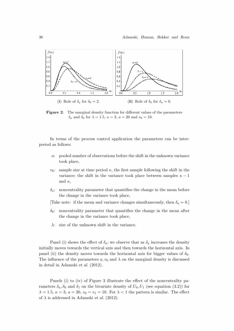
36 Adamski, Human, Bekker and Roux
(i) Role of δa for δ0 = 2. (ii) Role of δ0 for δa = 0.
Figure 2: The marginal density function for different values of the parameters
δa and δ0 for λ = 1.5, κ = 3, a = 20 and ν0 = 10.
In terms of the process control application the parameters can be inter-
preted as follows:
a: pooled number of observations before the shift in the unknown variance
took place,
v0: sample size at time period κ, the first sample following the shift in the
variance; the shift in the variance took place between samples κ − 1
and κ,
δa: noncentrality parameter that quantifies the change in the mean before
the change in the variance took place,
[Take note: if the mean and variance changes simultaneously, then δa = 0.]
δ0: noncentrality parameter that quantifies the change in the mean after
the change in the variance took place,
λ: size of the unknown shift in the variance.
Panel (i) shows the effect of δa; we observe that as δa increases the density
initially moves towards the vertical axis and then towards the horizontal axis. In
panel (ii) the density moves towards the horizontal axis for bigger values of δ0.
The influence of the parameters a, v0 and λ on the marginal density is discussed
in detail in Adamski et al. (2012).
Panels (i) to (iv) of Figure 3 illustrate the effect of the noncentrality pa-
rameters δa, δ0 and δ1 on the bivariate density of U0, U1 (see equation (3.2)) for
λ = 1.5, κ = 3, a = 20, v0 = v1 = 10. For λ < 1 the pattern is similar. The effect
of λ is addressed in Adamski et al. (2012).
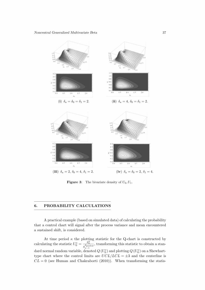
Noncentral Generalized Multivariate Beta 37
(i) δa = δ0 = δ1 = 2. (ii) δa = 4, δ0 = δ1 = 2.
(iii) δa = 2, δ0 = 4, δ1 = 2. (iv) δa = δ0 = 2, δ1 = 4.
Figure 3: The bivariate density of U0, U1.
6. PROBABILITY CALCULATIONS
A practical example (based on simulated data) of calculating the probability
that a control chart will signal after the process variance and mean encountered
a sustained shift, is considered.
At time period κ the plotting statistic for the Q-chart is constructed by
calculating the statistic U∗0 =
S2κ
S2pooledκ−1
, transforming this statistic to obtain a stan-
dard normal random variable, denoted Q (U∗0 ) and plotting Q (U∗
0 ) on a Shewhart-
type chart where the control limits are UCL/LCL = ±3 and the centerline is
CL = 0 (see Human and Chakraborti (2010)). When transforming the statis-
38 Adamski, Human, Bekker and Roux
tic to a normal random variable, Q-charts make use of the classical probability
integral transformation theorem (see Quesenberry (1991)).
The marginal density of U0 can be used to determine the probability of
detecting the shift in the process variance immediately, i.e. when collecting the
first sample after the shift took place. Once a shift in the process parameter
occurred, the run-length is the number of samples collected from time κ (i.e. first
sample after the change) until an out-of-control signal is observed (i.e. a plotting
statistic plots on or outside the control limits). The discrete random variable
defining the run-length is called the run-length random variable and typically
denoted by N . The distribution of N is called the run-length distribution. The
probability of detecting a shift immediately, in other words, the probability of
a run-length of one, is the likelihood that a signal is obtained at time κ. The
probability that the run-length is one, is one minus the probability that the
random variable, U∗0 , plots between the control limits,
(6.1) Pr(N = 1) = 1 −∫ UCL
LCLf(u∗
0) du∗0 = 1 −
∫ UCLκ
LCLκ
f(u0) du0 .
Take note that the difference between the random variables U∗0 and U0 (refer to
the definitions on page 7 and 8 of the introduction) will be incorporated in the
control limits of the control chart.
When the process is in-control, i.e. λ = 1 and the process mean did not en-
counter a shift, U∗0 =
W0/nκ
X/∑κ−1
i=1 ni
∼ F(nκ,∑κ−1
i=1 ni
), then the Q plotting statistic
is given by Q (U∗0 ) = Φ
−1[F (U∗
0 )] and the control limits UCLκ and LCLκ are
determined as follows:
−3 < Φ−1
[F (U∗0 )] < 3
⇐⇒ Φ (−3) < F (U∗0 ) < Φ (3)
⇐⇒ F−1[Φ (−3)] < U∗
0 < F−1[Φ (3)]
⇐⇒ F−1[Φ (−3)]
∑κ−1i=1 ni
nκ
< U0 <F−1
[Φ (3)]∑κ−1
i=1 ni
nκ
where
F (·) denotes the cumulative distribution function of the F distribution,
F−1(·) denotes the inverse of the cumulative distribution function of the
F distribution,
Φ (·) denotes the standard normal cumulative distribution function,
Φ−1
(·) denotes the inverse of the standard normal cumulative distribution
function.
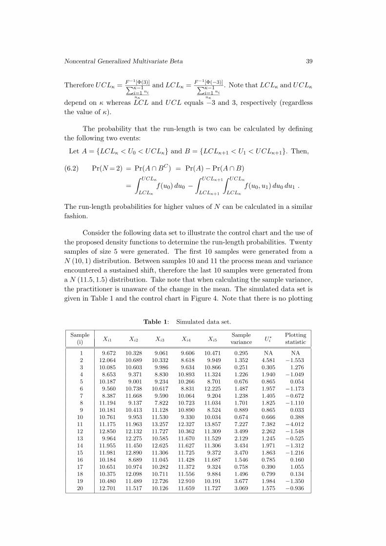
Noncentral Generalized Multivariate Beta 39
Therefore UCLκ =F−1[Φ(3)]∑κ−1
i=1 ni
nκ
and LCLκ =F−1[Φ(−3)]∑κ−1
i=1 ni
nκ
. Note that LCLκ and UCLκ
depend on κ whereas LCL and UCL equals −3 and 3, respectively (regardless
the value of κ).
The probability that the run-length is two can be calculated by defining
the following two events:
Let A = {LCLκ < U0 < UCLκ} and B = {LCLκ+1 < U1 < UCLκ+1}. Then,
Pr(N = 2) = Pr(A ∩ BC) = Pr(A) − Pr(A ∩ B)(6.2)
=
∫ UCLκ
LCLκ
f(u0) du0 −∫ UCLκ+1
LCLκ+1
∫ UCLκ
LCLκ
f(u0, u1) du0 du1 .
The run-length probabilities for higher values of N can be calculated in a similar
fashion.
Consider the following data set to illustrate the control chart and the use of
the proposed density functions to determine the run-length probabilities. Twenty
samples of size 5 were generated. The first 10 samples were generated from a
N (10, 1) distribution. Between samples 10 and 11 the process mean and variance
encountered a sustained shift, therefore the last 10 samples were generated from
a N (11.5, 1.5) distribution. Take note that when calculating the sample variance,
the practitioner is unaware of the change in the mean. The simulated data set is
given in Table 1 and the control chart in Figure 4. Note that there is no plotting
Table 1: Simulated data set.
Sample Sample Plotting(i)
Xi1 Xi2 Xi3 Xi4 Xi5 varianceU
∗
i statistic
1 9.672 10.328 9.061 9.606 10.471 0.295 NA NA2 12.064 10.689 10.332 8.618 9.949 1.352 4.581 −1.5533 10.085 10.603 9.986 9.634 10.866 0.251 0.305 1.2764 8.653 9.371 8.830 10.893 11.324 1.226 1.940 −1.0495 10.187 9.001 9.234 10.266 8.701 0.676 0.865 0.0546 9.560 10.738 10.617 8.831 12.225 1.487 1.957 −1.1737 8.387 11.668 9.590 10.064 9.204 1.238 1.405 −0.6728 11.194 9.137 7.822 10.723 11.034 1.701 1.825 −1.1109 10.181 10.413 11.128 10.890 8.524 0.889 0.865 0.033
10 10.761 9.953 11.530 9.330 10.034 0.674 0.666 0.38811 11.175 11.963 13.257 12.327 13.857 7.227 7.382 −4.01212 12.850 12.132 11.727 10.362 11.309 3.499 2.262 −1.54813 9.964 12.275 10.585 11.670 11.529 2.129 1.245 −0.52514 11.955 11.450 12.625 11.627 11.306 3.434 1.971 −1.31215 11.981 12.890 11.306 11.725 9.372 3.470 1.863 −1.21616 10.184 8.689 11.045 11.428 11.687 1.546 0.785 0.16017 10.651 10.974 10.282 11.372 9.324 0.758 0.390 1.05518 10.375 12.098 10.711 11.556 9.884 1.496 0.799 0.13419 10.480 11.489 12.726 12.910 10.191 3.677 1.984 −1.35020 12.701 11.517 10.126 11.659 11.727 3.069 1.575 −0.936
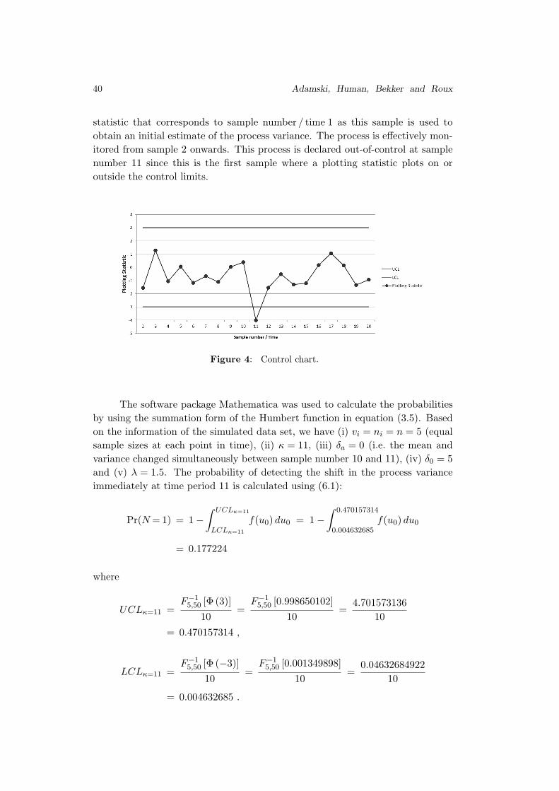
40 Adamski, Human, Bekker and Roux
statistic that corresponds to sample number / time 1 as this sample is used to
obtain an initial estimate of the process variance. The process is effectively mon-
itored from sample 2 onwards. This process is declared out-of-control at sample
number 11 since this is the first sample where a plotting statistic plots on or
outside the control limits.
Figure 4: Control chart.
The software package Mathematica was used to calculate the probabilities
by using the summation form of the Humbert function in equation (3.5). Based
on the information of the simulated data set, we have (i) vi = ni = n = 5 (equal
sample sizes at each point in time), (ii) κ = 11, (iii) δa = 0 (i.e. the mean and
variance changed simultaneously between sample number 10 and 11), (iv) δ0 = 5
and (v) λ = 1.5. The probability of detecting the shift in the process variance
immediately at time period 11 is calculated using (6.1):
Pr(N = 1) = 1 −∫ UCLκ=11
LCLκ=11
f(u0) du0 = 1 −∫ 0.470157314
0.004632685f(u0) du0
= 0.177224
where
UCLκ=11 =F−1
5,50 [Φ (3)]
10=
F−15,50 [0.998650102]
10=
4.701573136
10
= 0.470157314 ,
LCLκ=11 =F−1
5,50 [Φ (−3)]
10=
F−15,50 [0.001349898]
10=
0.04632684922
10
= 0.004632685 .
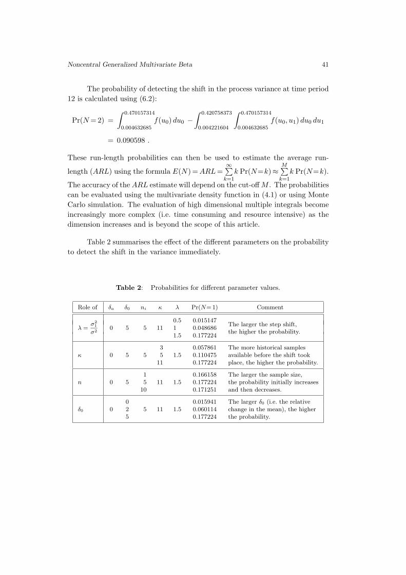
Noncentral Generalized Multivariate Beta 41
The probability of detecting the shift in the process variance at time period
12 is calculated using (6.2):
Pr(N = 2) =
∫ 0.470157314
0.004632685f(u0) du0 −
∫ 0.420758373
0.004221604
∫ 0.470157314
0.004632685f(u0, u1) du0 du1
= 0.090598 .
These run-length probabilities can then be used to estimate the average run-
length (ARL) using the formula E(N) = ARL =
∞∑k=1
k Pr(N=k)≈M∑
k=1
k Pr(N=k).
The accuracy of the ARL estimate will depend on the cut-off M . The probabilities
can be evaluated using the multivariate density function in (4.1) or using Monte
Carlo simulation. The evaluation of high dimensional multiple integrals become
increasingly more complex (i.e. time consuming and resource intensive) as the
dimension increases and is beyond the scope of this article.
Table 2 summarises the effect of the different parameters on the probability
to detect the shift in the variance immediately.
Table 2: Probabilities for different parameter values.
Role of δa δ0 ni κ λ Pr(N= 1) Comment
0.5 0.015147The larger the step shift,
λ =σ
21
σ20 5 5 11 1 0.048686
the higher the probability.1.5 0.177224
3 0.057861 The more historical samplesκ 0 5 5 5 1.5 0.110475 available before the shift took
11 0.177224 place, the higher the probability.
1 0.166158 The larger the sample size,n 0 5 5 11 1.5 0.177224 the probability initially increases
10 0.171251 and then decreases.
0 0.015941 The larger δ0 (i.e. the relativeδ0 0 2 5 11 1.5 0.060114 change in the mean), the higher
5 0.177224 the probability.

42 Adamski, Human, Bekker and Roux
7. CONCLUDING REMARKS
Adamski et al. (2012) recently introduced a new generalized multivariate
beta distribution with density in closed form, where a distribution is needed for
the run-length of a Q-chart that monitors the process mean when measurements
are from an exponential distribution with unknown parameter. In this paper the
distributions are proposed for the case when measurements from each sample
are independent and identically distributed normal random variables and we are
monitoring the unknown spread when the known mean encountered a sustained
shift. We have generalized the proposed model to the multivariate case and we
hope that the results presented in this paper will be useful in the Statistical
Process Control field.
ACKNOWLEDGMENTS
This work is based upon research supported by the National Research Foun-
dation, South Africa (Grant: FA2007043000003 and the Thuthuka programme:
TTK20100707000011868). We also acknowledge the valuable suggestions from
Professor Filipe Marques and the anonymous referees whom helped in approving
this paper.
REFERENCES
[1] Adamski, K.; Human, S.W. and Bekker, A. (2012). A generalized multi-
variate beta distribution: control charting when the measurements are from an
exponential distribution, Statistical Papers, 53, 1045–1064.
[2] Gradshteyn, I.S. and Ryzhik, I.M. (2007). Table of Integrals, Series, and
Products, Academic Press, Amsterdam.
[3] Gupta, A.K.; Orozco-Castaneda, J.M. and Nagar, D.K. (2009). Non-
central bivariate beta distribution, Statistical Papers, 52, 139–152.
[4] Human, S.W. and Chakraborti, S. (2010). Q charts for the exponential distri-
bution, JSM 2010 Proceedings, Section On Quality And Productivity, Vancouver,
British Columbia, Canada.
[5] Johnson, N.L.; Kotz, S. and Balakrishnan, N. (1995). Continuous Uni-
variate Distributions, Vol. 2 (second edition), John Wiley & Sons, New York.

Noncentral Generalized Multivariate Beta 43
[6] Mathai, A.M. (1993). A Handbook Of Generalized Special Functions For Sta-
tistical And Physical Sciences, Clarendon Press, Oxford.
[7] Montgomery, D.C. (2009). Statistical Quality Control: A Modern Introduc-
tion, 6th
ed., John Wiley, New York.
[8] Quesenberry, C.P. (1991). SPC Q Charts for start-up processes and short or
long runs, Journal Of Quality Technology, 23(3), 213–224.
[9] Patnaik, J.H. (1949). The non-central χ2and F -distributions and their appli-
cations, Biometrika, 36, 202–232.
[10] Pe, T. and Drygas, H. (2006). An alternative representation of noncentral beta
and F distributions, Statistical Papers, 47, 311–318.
[11] Prudnikov, A.P.; Brychkov, Y.A. and Marichev, O.I. (1986). Integrals
and Series, Volume I: Elementary Functions, Gordon and Breach, New York.
[12] Sanchez, L.E. and Nagar, D.K. (2003). Non-central matrix-variate Dirichlet
distribution, Taiwanese Journal Of Mathematics, 7(3), 477–491.
[13] Sanchez, L.E.; Nagar, D.K. and Gupta, A.K. (2006). Properties of noncen-
tral Dirichlet distributions, Computers and Mathematics with Applications, 52,
1671–1682.
[14] Srivastava, H.M. and Kashyap, B.R.K. (1982). Special Functions in Queuing
Theory And Related Stochastic Processes, Academic Press, New York.
[15] Tang, P.C. (1938). The power function of the analysis of variance tests with
tables and illustrations of their use, Statistical Research Memoirs, 2, 126–150.
[16] Troskie, C.G. (1967). Noncentral multivariate Dirichlet distributions, South
African Statistical Journal, 1, 21–32.

REVSTAT – Statistical Journal
Volume 11, Number 1, March 2013, 45–65
USE OF SURVIVAL MODELS IN A REFINERY
Authors: Sılvia Madeira
– Phd in Mathematics, ECT of University of Evora, Portugal
Paulo Infante
– CIMA/DMAT, ECT of University of Evora, Portugal
Filipe Didelet
– EST, IPS Setubal, Portugal
Abstract:
• Statistical methods are nowadays increasingly useful in industrial engineering. From
plant design reliability to equipment analysis, there is much to cover with statistical
models in order to improve the efficiency of systems. At Sines refinery we found it
useful to apply a Cox model to a particular critical equipment trying to find process
variables that cause its vibration as well as to apply well known distributions to
baseline hazard rate.
Key-Words:
• reliability; maintenance; time between failures; Kaplan–Meier; Cox proportional
hazards.
AMS Subject Classification:
• 62N01, 62P30, 90B25.

46 Sılvia Madeira, Paulo Infante and Filipe Didelet
Use of Survival Models in a Refinery 47
1. INTRODUCTION
As industries became more competitive, their methods to improve results
are intimately related to efficiency. Although efficiency can be achieved with
technology, it only can be reliable based on the fact that the system is prepared
for failures, managing them the best way. Failures can be classified as follows:
avoided, predictable or inevitable. In each case, knowing equipment behaviour
helps companies to manage spare parts, man-hours and maintenance issues that
will improve reliability and save money [12]. Reliability studies are then a priority
and this work has been written to support decisions based on reliability models
and according to standards [8].
Sines refinery has been concerned with the shut-downs made by the Turbo-
Expander equipment in the FCC unit (Fluid Catalytic Cracking). As it was
having problems due to a vibration failure mode causing FCC unit shut-down
since year 2000, it was decided to investigate the origin of the vibration. Ex-
pander manufacturers and other entities that have this kind of equipment have
investigated this problem as it is a big economical issue for the companies as we
can see in [4] and [6]. They highly recommend investigating efficiency in order to
detect scaling deposition in expander rotor blades. It is believed that the com-
position of some particles resulting from process reaction are the key for scaling,
not just erosion. On 2011 turnaround, the procedure of changing the expander’s
rotor and shroud was not complete. Only the rotor was changed. This has caused
a slight gap between the shroud and the rotor blades due to shroud erosion. This
gap is believed to cause less resistance and then, less particles deposition. How-
ever, results of Cox Proportional Hazards [2] [3] demonstrate components in these
particles to be linked with high values of expander vibration and with times to
failure. In Section 3 we have a brief description of the equipment and contextu-
alization of the subject. In Section 4 we will refer to the goal of this work and
variables definition. Then we will present some parametric and non-parametric
approaches using Kaplan–Meier estimator and Cox Proportional Hazards in Sec-
tion 5, and a parametric adjustment to the null model with parametric models.
Finally, Section 6 is dedicated to some general considerations of this work.
2. MODELS
Several approaches were tried and reviews for different models were stud-
ied, although not all of them could fit on the data and conditions of our study.
Cox Proportional Hazards had a strong focus because of its flexibility, but some
approaches using Competing Risks Theory as we can see in Fine and Gray [5]
or Lunn and McNeil [11] were not possible due the complexity of the system.
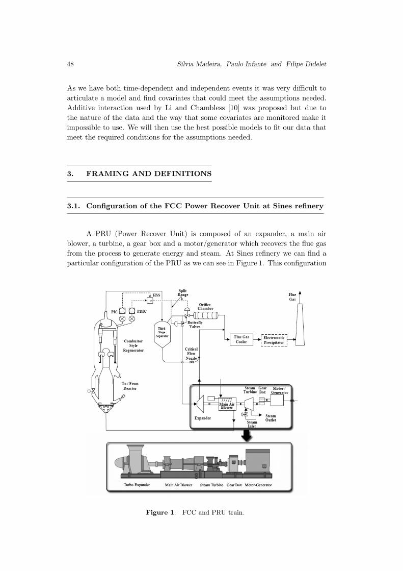
48 Sılvia Madeira, Paulo Infante and Filipe Didelet
As we have both time-dependent and independent events it was very difficult to
articulate a model and find covariates that could meet the assumptions needed.
Additive interaction used by Li and Chambless [10] was proposed but due to
the nature of the data and the way that some covariates are monitored make it
impossible to use. We will then use the best possible models to fit our data that
meet the required conditions for the assumptions needed.
3. FRAMING AND DEFINITIONS
3.1. Configuration of the FCC Power Recover Unit at Sines refinery
A PRU (Power Recover Unit) is composed of an expander, a main air
blower, a turbine, a gear box and a motor/generator which recovers the flue gas
from the process to generate energy and steam. At Sines refinery we can find a
particular configuration of the PRU as we can see in Figure 1. This configuration
Figure 1: FCC and PRU train.
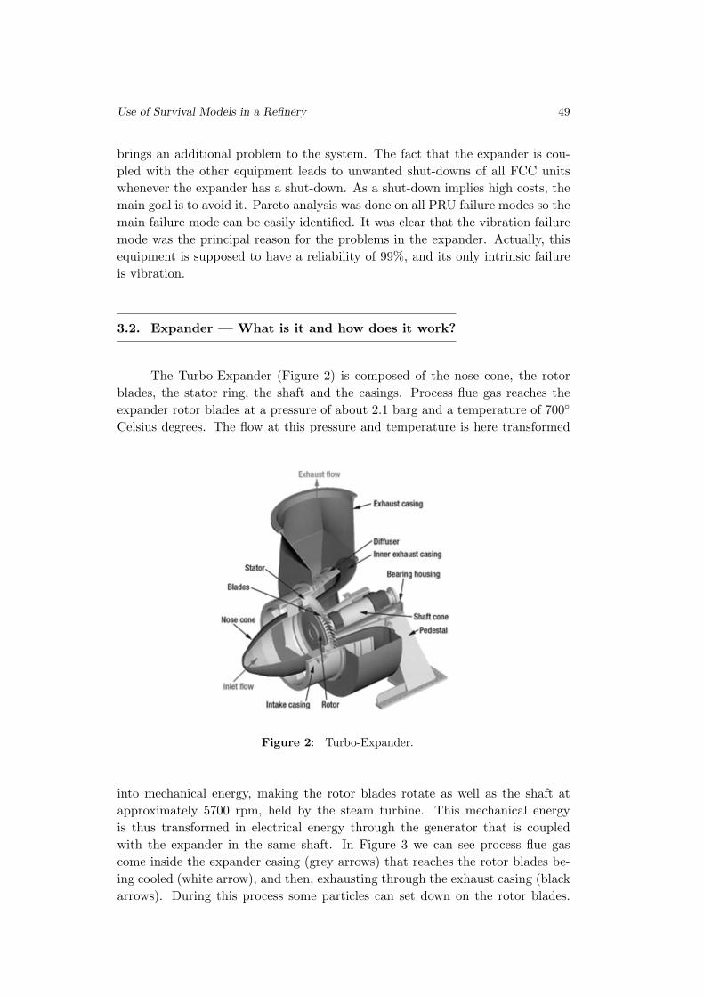
Use of Survival Models in a Refinery 49
brings an additional problem to the system. The fact that the expander is cou-
pled with the other equipment leads to unwanted shut-downs of all FCC units
whenever the expander has a shut-down. As a shut-down implies high costs, the
main goal is to avoid it. Pareto analysis was done on all PRU failure modes so the
main failure mode can be easily identified. It was clear that the vibration failure
mode was the principal reason for the problems in the expander. Actually, this
equipment is supposed to have a reliability of 99%, and its only intrinsic failure
is vibration.
3.2. Expander — What is it and how does it work?
The Turbo-Expander (Figure 2) is composed of the nose cone, the rotor
blades, the stator ring, the shaft and the casings. Process flue gas reaches the
expander rotor blades at a pressure of about 2.1 barg and a temperature of 700◦
Celsius degrees. The flow at this pressure and temperature is here transformed
Figure 2: Turbo-Expander.
into mechanical energy, making the rotor blades rotate as well as the shaft at
approximately 5700 rpm, held by the steam turbine. This mechanical energy
is thus transformed in electrical energy through the generator that is coupled
with the expander in the same shaft. In Figure 3 we can see process flue gas
come inside the expander casing (grey arrows) that reaches the rotor blades be-
ing cooled (white arrow), and then, exhausting through the exhaust casing (black
arrows). During this process some particles can set down on the rotor blades.
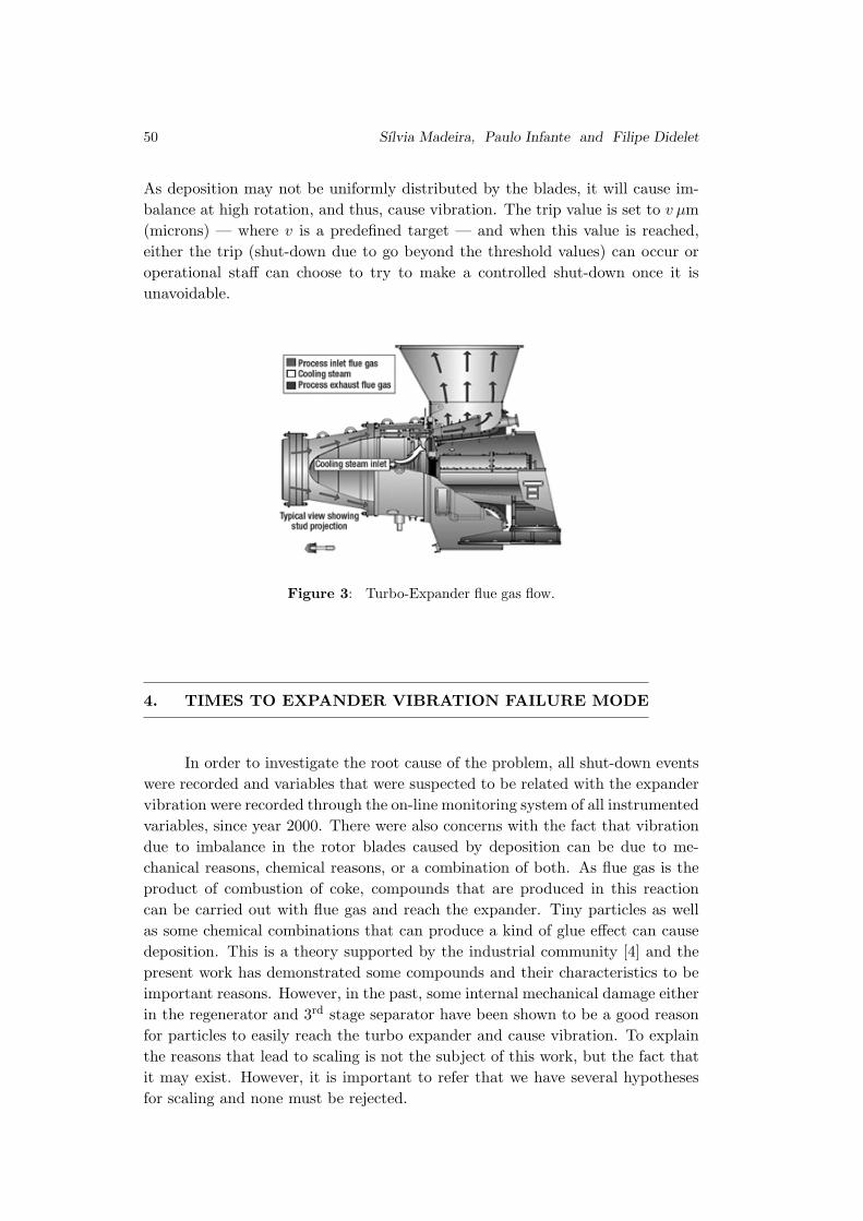
50 Sılvia Madeira, Paulo Infante and Filipe Didelet
As deposition may not be uniformly distributed by the blades, it will cause im-
balance at high rotation, and thus, cause vibration. The trip value is set to v µm
(microns) — where v is a predefined target — and when this value is reached,
either the trip (shut-down due to go beyond the threshold values) can occur or
operational staff can choose to try to make a controlled shut-down once it is
unavoidable.
Figure 3: Turbo-Expander flue gas flow.
4. TIMES TO EXPANDER VIBRATION FAILURE MODE
In order to investigate the root cause of the problem, all shut-down events
were recorded and variables that were suspected to be related with the expander
vibration were recorded through the on-line monitoring system of all instrumented
variables, since year 2000. There were also concerns with the fact that vibration
due to imbalance in the rotor blades caused by deposition can be due to me-
chanical reasons, chemical reasons, or a combination of both. As flue gas is the
product of combustion of coke, compounds that are produced in this reaction
can be carried out with flue gas and reach the expander. Tiny particles as well
as some chemical combinations that can produce a kind of glue effect can cause
deposition. This is a theory supported by the industrial community [4] and the
present work has demonstrated some compounds and their characteristics to be
important reasons. However, in the past, some internal mechanical damage either
in the regenerator and 3rd
stage separator have been shown to be a good reason
for particles to easily reach the turbo expander and cause vibration. To explain
the reasons that lead to scaling is not the subject of this work, but the fact that
it may exist. However, it is important to refer that we have several hypotheses
for scaling and none must be rejected.
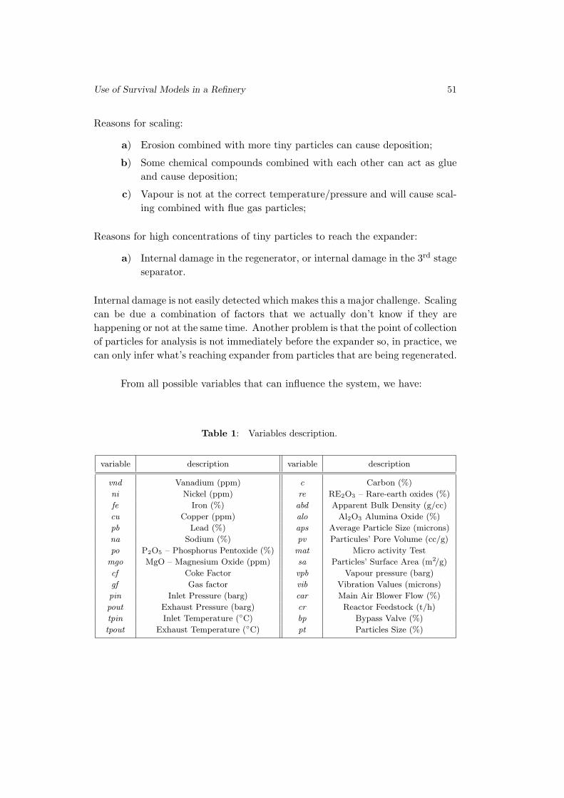
Use of Survival Models in a Refinery 51
Reasons for scaling:
a) Erosion combined with more tiny particles can cause deposition;
b) Some chemical compounds combined with each other can act as glue
and cause deposition;
c) Vapour is not at the correct temperature/pressure and will cause scal-
ing combined with flue gas particles;
Reasons for high concentrations of tiny particles to reach the expander:
a) Internal damage in the regenerator, or internal damage in the 3rd
stage
separator.
Internal damage is not easily detected which makes this a major challenge. Scaling
can be due a combination of factors that we actually don’t know if they are
happening or not at the same time. Another problem is that the point of collection
of particles for analysis is not immediately before the expander so, in practice, we
can only infer what’s reaching expander from particles that are being regenerated.
From all possible variables that can influence the system, we have:
Table 1: Variables description.
variable description variable description
vnd Vanadium (ppm) c Carbon (%)
ni Nickel (ppm) re RE2O3 – Rare-earth oxides (%)
fe Iron (%) abd Apparent Bulk Density (g/cc)
cu Copper (ppm) alo Al2O3 Alumina Oxide (%)
pb Lead (%) aps Average Particle Size (microns)
na Sodium (%) pv Particules’ Pore Volume (cc/g)
po P2O5 – Phosphorus Pentoxide (%) mat Micro activity Test
mgo MgO – Magnesium Oxide (ppm) sa Particles’ Surface Area (m2/g)
cf Coke Factor vpb Vapour pressure (barg)
gf Gas factor vib Vibration Values (microns)
pin Inlet Pressure (barg) car Main Air Blower Flow (%)
pout Exhaust Pressure (barg) cr Reactor Feedstock (t/h)
tpin Inlet Temperature (◦C) bp Bypass Valve (%)
tpout Exhaust Temperature (◦C) pt Particles Size (%)
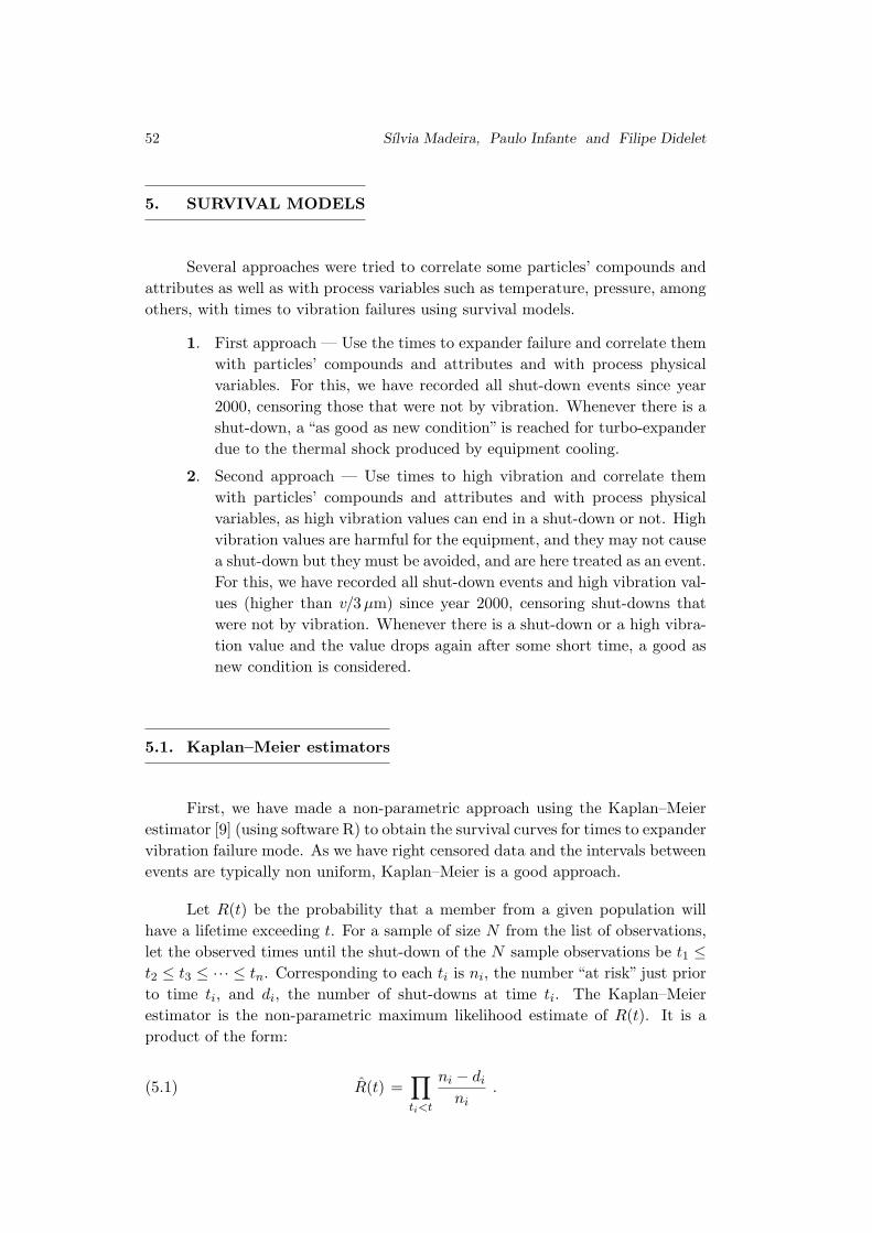
52 Sılvia Madeira, Paulo Infante and Filipe Didelet
5. SURVIVAL MODELS
Several approaches were tried to correlate some particles’ compounds and
attributes as well as with process variables such as temperature, pressure, among
others, with times to vibration failures using survival models.
1. First approach — Use the times to expander failure and correlate them
with particles’ compounds and attributes and with process physical
variables. For this, we have recorded all shut-down events since year
2000, censoring those that were not by vibration. Whenever there is a
shut-down, a “as good as new condition” is reached for turbo-expander
due to the thermal shock produced by equipment cooling.
2. Second approach — Use times to high vibration and correlate them
with particles’ compounds and attributes and with process physical
variables, as high vibration values can end in a shut-down or not. High
vibration values are harmful for the equipment, and they may not cause
a shut-down but they must be avoided, and are here treated as an event.
For this, we have recorded all shut-down events and high vibration val-
ues (higher than v/3 µm) since year 2000, censoring shut-downs that
were not by vibration. Whenever there is a shut-down or a high vibra-
tion value and the value drops again after some short time, a good as
new condition is considered.
5.1. Kaplan–Meier estimators
First, we have made a non-parametric approach using the Kaplan–Meier
estimator [9] (using software R) to obtain the survival curves for times to expander
vibration failure mode. As we have right censored data and the intervals between
events are typically non uniform, Kaplan–Meier is a good approach.
Let R(t) be the probability that a member from a given population will
have a lifetime exceeding t. For a sample of size N from the list of observations,
let the observed times until the shut-down of the N sample observations be t1 ≤t2 ≤ t3 ≤ ··· ≤ tn. Corresponding to each ti is ni, the number “at risk” just prior
to time ti, and di, the number of shut-downs at time ti. The Kaplan–Meier
estimator is the non-parametric maximum likelihood estimate of R(t). It is a
product of the form:
(5.1) R(t) =
∏
ti<t
ni − di
ni.
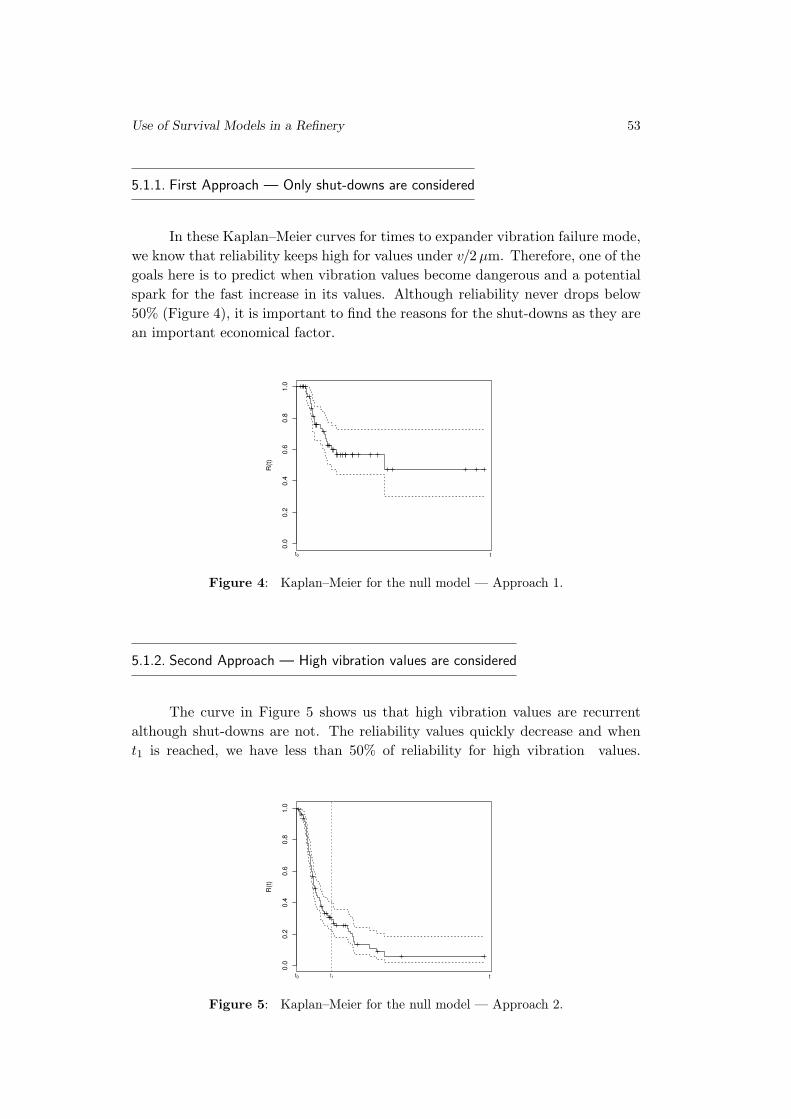
Use of Survival Models in a Refinery 53
5.1.1. First Approach — Only shut-downs are considered
In these Kaplan–Meier curves for times to expander vibration failure mode,
we know that reliability keeps high for values under v/2 µm. Therefore, one of the
goals here is to predict when vibration values become dangerous and a potential
spark for the fast increase in its values. Although reliability never drops below
50% (Figure 4), it is important to find the reasons for the shut-downs as they are
an important economical factor.
0.0
0.2
0.4
0.6
0.8
1.0
R(t
)
t0 t
Figure 4: Kaplan–Meier for the null model — Approach 1.
5.1.2. Second Approach — High vibration values are considered
The curve in Figure 5 shows us that high vibration values are recurrent
although shut-downs are not. The reliability values quickly decrease and when
t1 is reached, we have less than 50% of reliability for high vibration values.
0.0
0.2
0.4
0.6
0.8
1.0
R(t
)
t0 tt1
Figure 5: Kaplan–Meier for the null model — Approach 2.
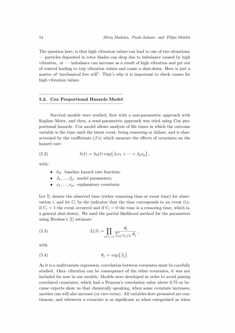
54 Sılvia Madeira, Paulo Infante and Filipe Didelet
The question here, is that high vibration values can lead to one of two situations:
— particles deposited in rotor blades can drop due to imbalance caused by high
vibration, or — imbalance can increase as a result of high vibration and get out
of control leading to trip vibration values and cause a shut-down. Here is just a
matter of “mechanical free will”. That’s why it is important to check causes for
high vibration values.
5.2. Cox Proportional Hazards Model
Survival models were studied, first with a non-parametric approach with
Kaplan–Meier, and then, a semi-parametric approach was tried using Cox pro-
portional hazards. Cox model allows analysis of life times in which the outcome
variable is the time until the latest event, being censoring or failure, and is char-
acterised by the coefficients (β’s) which measure the effects of covariates on the
hazard rate:
(5.2) h(t) = h0(t) exp{β1x1 + ··· + βpxp
},
with:
• h0: baseline hazard rate function;
• β1, ..., βp: model parameters;
• x1, ..., xp: explanatory covariates.
Let Yi denote the observed time (either censoring time or event time) for obser-
vation i, and let Ci be the indicator that the time corresponds to an event (i.e.
if Ci = 1 the event occurred and if Ci = 0 the time is a censoring time, which is,
a general shut-down). We used the partial likelihood method for the parameters
using Breslow’s [1] estimate:
(5.3) L(β) =
∏
i:Ci=1
θi∑j:Yj≤Yi
θj,
with
(5.4) θj = exp{βj
}
As it is a multivariate regression, correlation between covariates must be carefully
studied. Once vibration can be consequence of the other covariates, it was not
included for now in our models. Models were developed in order to avoid joining
correlated covariates, which had a Pearson’s correlation value above 0.75 or be-
cause experts show us that chemically speaking, when some covariate increases,
another one will also increase (or vice-versa). All variables here presented are con-
tinuous, and whenever a covariate is as significant as when categorized as when
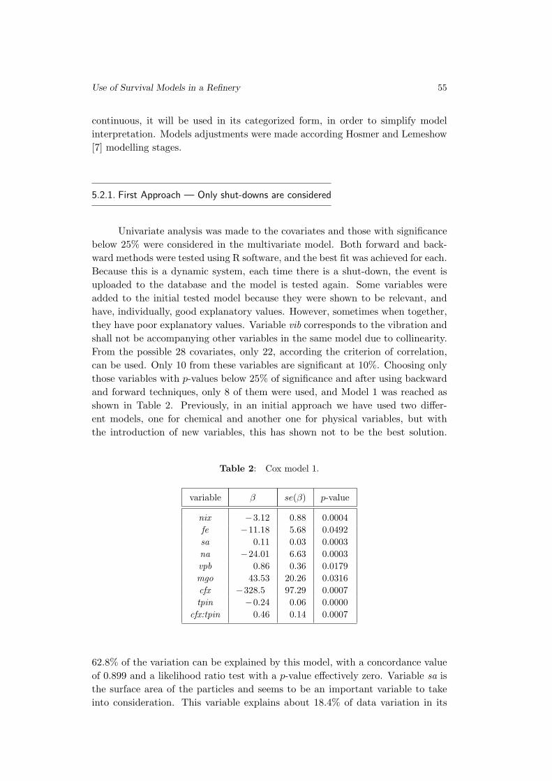
Use of Survival Models in a Refinery 55
continuous, it will be used in its categorized form, in order to simplify model
interpretation. Models adjustments were made according Hosmer and Lemeshow
[7] modelling stages.
5.2.1. First Approach — Only shut-downs are considered
Univariate analysis was made to the covariates and those with significance
below 25% were considered in the multivariate model. Both forward and back-
ward methods were tested using R software, and the best fit was achieved for each.
Because this is a dynamic system, each time there is a shut-down, the event is
uploaded to the database and the model is tested again. Some variables were
added to the initial tested model because they were shown to be relevant, and
have, individually, good explanatory values. However, sometimes when together,
they have poor explanatory values. Variable vib corresponds to the vibration and
shall not be accompanying other variables in the same model due to collinearity.
From the possible 28 covariates, only 22, according the criterion of correlation,
can be used. Only 10 from these variables are significant at 10%. Choosing only
those variables with p-values below 25% of significance and after using backward
and forward techniques, only 8 of them were used, and Model 1 was reached as
shown in Table 2. Previously, in an initial approach we have used two differ-
ent models, one for chemical and another one for physical variables, but with
the introduction of new variables, this has shown not to be the best solution.
Table 2: Cox model 1.
variable β se(β) p-value
nix −3.12 0.88 0.0004
fe −11.18 5.68 0.0492
sa 0.11 0.03 0.0003
na −24.01 6.63 0.0003
vpb 0.86 0.36 0.0179
mgo 43.53 20.26 0.0316
cfx −328.5 97.29 0.0007
tpin −0.24 0.06 0.0000
cfx:tpin 0.46 0.14 0.0007
62.8% of the variation can be explained by this model, with a concordance value
of 0.899 and a likelihood ratio test with a p-value effectively zero. Variable sa is
the surface area of the particles and seems to be an important variable to take
into consideration. This variable explains about 18.4% of data variation in its
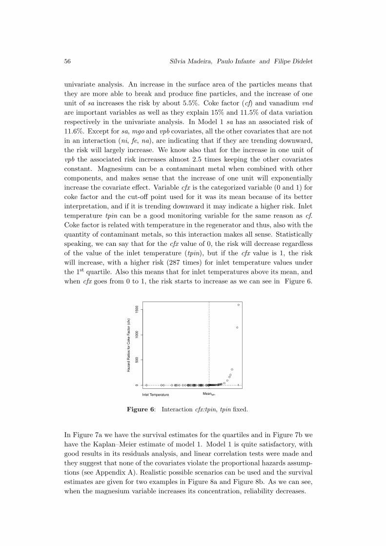
56 Sılvia Madeira, Paulo Infante and Filipe Didelet
univariate analysis. An increase in the surface area of the particles means that
they are more able to break and produce fine particles, and the increase of one
unit of sa increases the risk by about 5.5%. Coke factor (cf) and vanadium vnd
are important variables as well as they explain 15% and 11.5% of data variation
respectively in the univariate analysis. In Model 1 sa has an associated risk of
11.6%. Except for sa, mgo and vpb covariates, all the other covariates that are not
in an interaction (ni, fe, na), are indicating that if they are trending downward,
the risk will largely increase. We know also that for the increase in one unit of
vpb the associated risk increases almost 2.5 times keeping the other covariates
constant. Magnesium can be a contaminant metal when combined with other
components, and makes sense that the increase of one unit will exponentially
increase the covariate effect. Variable cfx is the categorized variable (0 and 1) for
coke factor and the cut-off point used for it was its mean because of its better
interpretation, and if it is trending downward it may indicate a higher risk. Inlet
temperature tpin can be a good monitoring variable for the same reason as cf.
Coke factor is related with temperature in the regenerator and thus, also with the
quantity of contaminant metals, so this interaction makes all sense. Statistically
speaking, we can say that for the cfx value of 0, the risk will decrease regardless
of the value of the inlet temperature (tpin), but if the cfx value is 1, the risk
will increase, with a higher risk (287 times) for inlet temperature values under
the 1st
quartile. Also this means that for inlet temperatures above its mean, and
when cfx goes from 0 to 1, the risk starts to increase as we can see in Figure 6.
05
00
10
00
15
00
Ha
za
rd R
atio
s fo
r C
oke
Fa
cto
r (c
fx)
Meantpin
1
Inlet Temperature
Figure 6: Interaction cfx:tpin, tpin fixed.
In Figure 7a we have the survival estimates for the quartiles and in Figure 7b we
have the Kaplan–Meier estimate of model 1. Model 1 is quite satisfactory, with
good results in its residuals analysis, and linear correlation tests were made and
they suggest that none of the covariates violate the proportional hazards assump-
tions (see Appendix A). Realistic possible scenarios can be used and the survival
estimates are given for two examples in Figure 8a and Figure 8b. As we can see,
when the magnesium variable increases its concentration, reliability decreases.
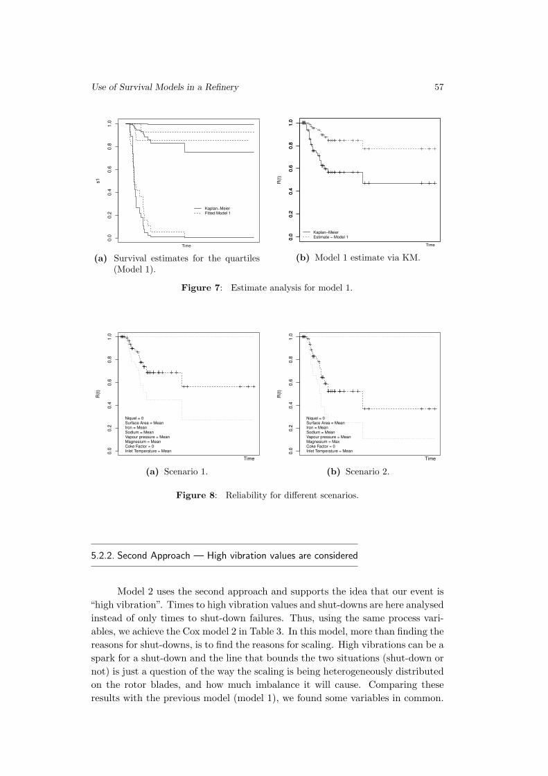
Use of Survival Models in a Refinery 57
0.0
0.2
0.4
0.6
0.8
1.0
s1
Kaplan−MeierFitted Model 1
Time
(a) Survival estimates for the quartiles
(Model 1).
0.0
0.2
0.4
0.6
0.8
1.0
0.0
0.2
0.4
0.6
0.8
1.0
R(t
)
Kaplan−MeierEstimate − Model 1
Time
(b) Model 1 estimate via KM.
Figure 7: Estimate analysis for model 1.
0.0
0.2
0.4
0.6
0.8
1.0
R(t
)
Niquel = 0Surface Area = MeanIron = MeanSodium = MeanVapour pressure = MeanMagnesium = MeanCoke Factor = 0Inlet Temperature = Mean
Time
(a) Scenario 1.
0.0
0.2
0.4
0.6
0.8
1.0
R(t
)
Niquel = 0Surface Area = MeanIron = MeanSodium = MeanVapour pressure = MeanMagnesium = MaxCoke Factor = 0Inlet Temperature = Mean
Time
(b) Scenario 2.
Figure 8: Reliability for different scenarios.
5.2.2. Second Approach — High vibration values are considered
Model 2 uses the second approach and supports the idea that our event is
“high vibration”. Times to high vibration values and shut-downs are here analysed
instead of only times to shut-down failures. Thus, using the same process vari-
ables, we achieve the Cox model 2 in Table 3. In this model, more than finding the
reasons for shut-downs, is to find the reasons for scaling. High vibrations can be a
spark for a shut-down and the line that bounds the two situations (shut-down or
not) is just a question of the way the scaling is being heterogeneously distributed
on the rotor blades, and how much imbalance it will cause. Comparing these
results with the previous model (model 1), we found some variables in common.
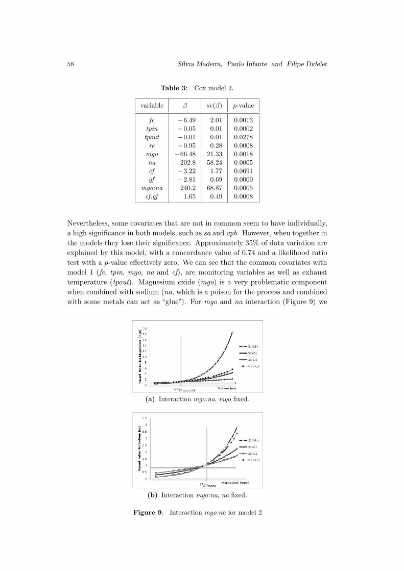
58 Sılvia Madeira, Paulo Infante and Filipe Didelet
Table 3: Cox model 2.
variable β se(β) p-value
fe −6.49 2.01 0.0013
tpin −0.05 0.01 0.0002
tpout −0.01 0.01 0.0278
re −0.95 0.28 0.0008
mgo −66.48 21.33 0.0018
na −202.8 58.24 0.0005
cf −3.22 1.77 0.0691
gf −2.81 0.69 0.0000
mgo:na 240.2 68.87 0.0005
cf:gf 1.65 0.49 0.0008
Nevertheless, some covariates that are not in common seem to have individually,
a high significance in both models, such as sa and vpb. However, when together in
the models they lose their significance. Approximately 35% of data variation are
explained by this model, with a concordance value of 0.74 and a likelihood ratio
test with a p-value effectively zero. We can see that the common covariates with
model 1 (fe, tpin, mgo, na and cf), are monitoring variables as well as exhaust
temperature (tpout). Magnesium oxide (mgo) is a very problematic component
when combined with sodium (na, which is a poison for the process and combined
with some metals can act as “glue”). For mgo and na interaction (Figure 9) we
(a) Interaction mgo:na, mgo fixed.
(b) Interaction mgo:na, na fixed.
Figure 9: Interaction mgo:na for model 2.
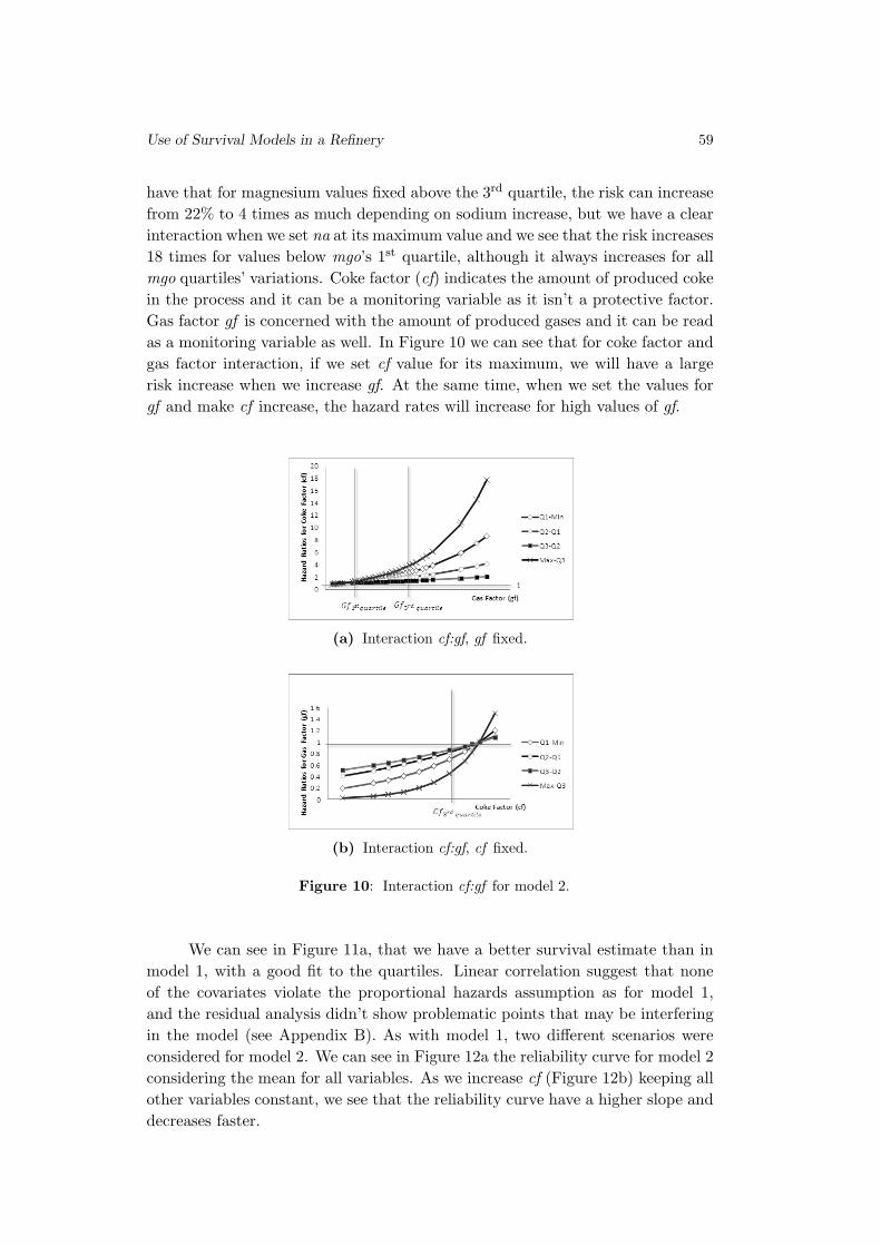
Use of Survival Models in a Refinery 59
have that for magnesium values fixed above the 3rd
quartile, the risk can increase
from 22% to 4 times as much depending on sodium increase, but we have a clear
interaction when we set na at its maximum value and we see that the risk increases
18 times for values below mgo’s 1st
quartile, although it always increases for all
mgo quartiles’ variations. Coke factor (cf) indicates the amount of produced coke
in the process and it can be a monitoring variable as it isn’t a protective factor.
Gas factor gf is concerned with the amount of produced gases and it can be read
as a monitoring variable as well. In Figure 10 we can see that for coke factor and
gas factor interaction, if we set cf value for its maximum, we will have a large
risk increase when we increase gf. At the same time, when we set the values for
gf and make cf increase, the hazard rates will increase for high values of gf.
(a) Interaction cf:gf, gf fixed.
(b) Interaction cf:gf, cf fixed.
Figure 10: Interaction cf:gf for model 2.
We can see in Figure 11a, that we have a better survival estimate than in
model 1, with a good fit to the quartiles. Linear correlation suggest that none
of the covariates violate the proportional hazards assumption as for model 1,
and the residual analysis didn’t show problematic points that may be interfering
in the model (see Appendix B). As with model 1, two different scenarios were
considered for model 2. We can see in Figure 12a the reliability curve for model 2
considering the mean for all variables. As we increase cf (Figure 12b) keeping all
other variables constant, we see that the reliability curve have a higher slope and
decreases faster.
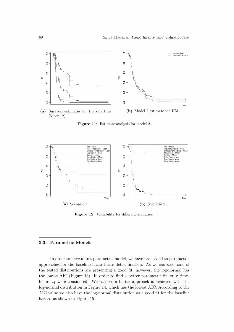
60 Sılvia Madeira, Paulo Infante and Filipe Didelet
0.0
0.2
0.4
0.6
0.8
1.0
s1
(a) Survival estimates for the quartiles
(Model 2).
0.0
0.2
0.4
0.6
0.8
1.0
0.0
0.2
0.4
0.6
0.8
1.0
R(t
)
Kaplan−MeierEstimate − Model 2
Time
(b) Model 2 estimate via KM.
Figure 11: Estimate analysis for model 2.
0.0
0.2
0.4
0.6
0.8
1.0
R(t
)
Iron = MeanInlet Temperature = MeanExhaust Temperature = MeanMagnesium = MeanSodium = MeanCoke Factor = MeanGas Factor = MeanRare Earth = Mean
Time
(a) Scenario 1.
0.0
0.2
0.4
0.6
0.8
1.0
R(t
)
Iron = MeanInlet Temperature = MeanExhaust Temperature = MeanMagnesium = MeanSodium = MeanCoke Factor = MaxGas Factor = MeanRare Earth = Mean
Time
(b) Scenario 2.
Figure 12: Reliability for different scenarios.
5.3. Parametric Models
In order to have a first parametric model, we have proceeded to parametric
approaches for the baseline hazard rate determination. As we can see, none of
the tested distributions are presenting a good fit, however, the log-normal has
the lowest AIC (Figure 13). In order to find a better parametric fit, only times
before t1 were considered. We can see a better approach is achieved with the
log-normal distribution in Figure 14, which has the lowest AIC. According to the
AIC value we also have the log-normal distribution as a good fit for the baseline
hazard as shown in Figure 15.
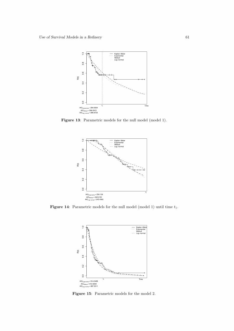
Use of Survival Models in a Refinery 61
0.0
0.2
0.4
0.6
0.8
1.0
R(t
)
Time
Kaplan−MeierExponentialWeibullLog−normal
AICExponential = 294.0934
AICWeibull = 296.0915
AICLog−normal = 286.9723
t1
Figure 13: Parametric models for the null model (model 1).
0.0
0.2
0.4
0.6
0.8
1.0
R(t
)
Kaplan−MeierExponentialWeibullLog−normal
AICExponential = 254.139
AICWeibull = 245.2191
AICLog−normal = 240.4093
t1
Figure 14: Parametric models for the null model (model 1) until time t1.
0.0
0.2
0.4
0.6
0.8
1.0
R(t
)
Time
Kaplan−MeierExponentialWeibullLog−normal
AICExponential = 914.5498
AICWeibull = 912.6094
AICLog−normal = 887.9311
t1
Figure 15: Parametric models for the model 2.

62 Sılvia Madeira, Paulo Infante and Filipe Didelet
6. CONCLUDING REMARKS
For the proposed problem in Section 4, the consistency of some covariates
in tested models make them a subject of investigation. Some covariates such
as surface area should be definitely monitored, as well as the inlet and exhaust
temperatures trend. It seems that sodium, magnesium and iron are influential
variables for the increase of the risk of high vibration values, and should be
monitored, although all these variables are very difficult to control as they depend
on the reactor feedstock and reactor temperatures. Investigation on this subject
will be ongoing as it can help to find the reasons for the so non-welcome shut-
downs. Future work will be done to mechanical equipment in order to optimize,
if possible, predictive maintenance scenarios.
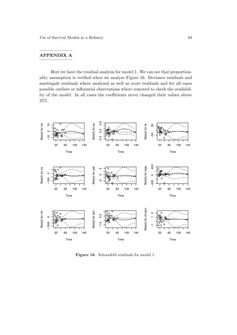
Use of Survival Models in a Refinery 63
APPENDIX A
Here we have the residual analysis for model 1. We can see that proportion-
ality assumption is verified when we analyse Figure 16. Deviance residuals and
martingale residuals where analysed as well as score residuals and for all cases
possible outliers or influential observations where removed to check the availabil-
ity of the model. In all cases the coefficients never changed their values above
25%.
20 60 100 140
−10
010
Time
Beta
(t)
for
nix
20 60 100 140
−0.4
0.2
0.8
Time
Beta
(t)
for
sa
20 60 100 140
−50
50
Time
Beta
(t)
for
fe
20 60 100 140
−100
0
Time
Beta
(t)
for
na
20 60 100 140
−2
26
Time
Beta
(t)
for
vpb
20 60 100 140
−400
0400
Time
Beta
(t)
for
mgo
20 60 100 140
−1500
0
Time
Beta
(t)
for
cfx
20 60 100 140
−1.0
0.0
Time
Beta
(t)
for
tpin
20 60 100 140
−1
12
Time
Beta
(t)
for
cfx
:tpin
Figure 16: Schoenfeld residuals for model 1.
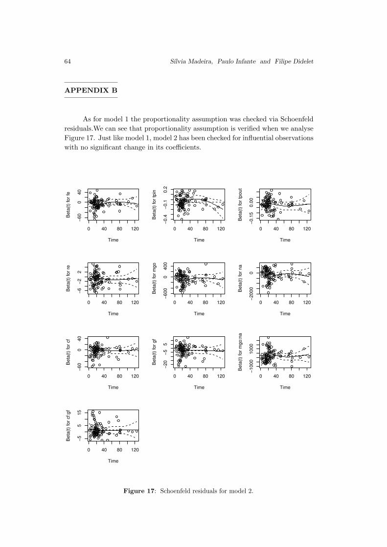
64 Sılvia Madeira, Paulo Infante and Filipe Didelet
APPENDIX B
As for model 1 the proportionality assumption was checked via Schoenfeld
residuals.We can see that proportionality assumption is verified when we analyse
Figure 17. Just like model 1, model 2 has been checked for influential observations
with no significant change in its coefficients.
0 40 80 120
−60
040
Time
Beta
(t)
for
fe
0 40 80 120
−0.4
−0.1
0.2
Time
Beta
(t)
for
tpin
0 40 80 120
−0.1
50.0
0
TimeB
eta
(t)
for
tpout
0 40 80 120
−6
−2
2
Time
Beta
(t)
for
re
0 40 80 120
−600
0400
Time
Beta
(t)
for
mgo
0 40 80 120
−2000
0
Time
Beta
(t)
for
na
0 40 80 120
−60
040
Time
Beta
(t)
for
cf
0 40 80 120
−20
−5
5
Time
Beta
(t)
for
gf
0 40 80 120
−1000
1000
Time
Beta
(t)
for
mgo:n
a
0 40 80 120
−5
515
Time
Beta
(t)
for
cf:gf
Figure 17: Schoenfeld residuals for model 2.
Use of Survival Models in a Refinery 65
ACKNOWLEDGMENTS
This study was supported on behalf of FCT (Portuguese Foundation for
Science and Technology) and Galp Energia, the insertion company for the PhD.
The second author is member of CIMA-UE, research center supported financially
by the FCT.
REFERENCES
[1] Breslow, N.E. (1972). Regression models and life tables (with discussion) by
D.R. Cox, Journal of the Royal Statistical Society, Series B, 34, 187–220.
[2] Cox, D.R. (1972). Regression models and life tables (with discussion), Journal
of the Royal Statistical Society, Series B, 34, 187–220.
[3] Cox, D.R. and Oakes, D. (1984). Analysis of Survival Data, Chapman and
Hall, London.
[4] Diangu, H. (2011). Analysis on causes of scaling in flue gas turbine of FCCU
and countermeasures, China Petroleum Processing and Petrochemical Technology,
13(1), 66–74.
[5] Fine, J.P. and Gray, R.J. (1999). A proportional hazards model for the sub-
distribution of a competing risk, Journal of the American Statistical Association,
94, 496–509.
[6] Gladys, N. and Laura, V. (1999). Analysis of rotor-blade failure due to high-
temperature corrosion/erosion, Surface and Coatings Technology, 120–121, 145–
150.
[7] Hosmer, D.W. and Lemeshow, S. (2000). Applied Logistic Regression, Wiley,
New York.
[8] ISO 14224:2006 (2006). Petroleum and Natural Gas Industries — Collection
and Exchange of Reliability and Maintenance Data for Equipment, International
Standard Organization, Second Edition.
[9] Kaplan, E.L. and Meier, P. (1958). Nonparametric estimation from incom-
plete observations, J. Amer. Statist. Assn., 53, 457–481.
[10] Li, R. and Chambless, L. (2007). Test for additive interaction in proportional
hazards models, Annals of Epidemiology, 17(3), 237–236.
[11] Lunn, M. and McNeil, D. (1995). Applying Cox regression to competing risks,
Biometrics, 51(2), 524–532.
[12] Rausand, M. and Hoyland, A. (2004). System Reliability Theory — Models,
Statistical Methods and Applications, Second Edition, Wiley.

REVSTAT – Statistical Journal
Volume 11, Number 1, March 2013, 67–82
ROBUST METHODS IN ACCEPTANCE SAMPLING
Authors: Elisabete Carolino
– Escola Superior de Tecnologias da Saude de Lisboa (IPL), Portugal
Isabel Barao
– Faculdade de Ciencias (UL), Portugal
Abstract:
• In the quality control of a production process (of goods or services), from a statistical
point of view, the focus is either on the process itself with application of Statistical
Process Control or on its frontiers, with application of Acceptance Sampling (AS) and
Experimental Design. AS is used to inspect either the process output (final product)
or the process input (raw material). The purpose of the design of a sampling plan is
to determine a course of action that, if applied to a series of lots of a given quality,
and based on sampling information, leads to a specified risk of accepting/rejecting
them. Thus AS yields quality assurance. The classic AS by variables is based on the
hypothesis that the observed quality characteristics follow the Gaussian distribution
(treated in classical standards). This is sometimes an abusive assumption that leads
to wrong decisions. AS for non-Gaussian variables, mainly for variables with asym-
metric and/or heavy tailed distributions, is a relevant topic. When we have a known
non-Gaussian distribution we can build specific AS plans associated with that distri-
bution. Alternatively, we can use the Gaussian classical plans with robust estimators
of location and scale — for example, the total median and the sample median as
location estimates, and the full range, the sample range and the interquartile range,
as scale estimates. In this work we will address the problem of determining AS plans
by variables for Extreme Value distributions (Weibull and Frechet) with known shape
parameter. Classical plans, specific plans and plans using the robust estimates for
location are determined and compared.
Key-Words:
• quality control; acceptance sampling; acceptance sampling by variables; robust methods.

68 Carolino and Barao
Robust Methods in AS 69
1. INTRODUCTION
Acceptance Sampling (AS) is used to inspect either the output process —
final product — or the input — initial product. On a lot-by-lot basis, a random
sample is taken from the lot and based on the information given by the sample a
decision is taken: to accept or to reject the lot. The purpose of AS is to determine
a course of action, not to estimate lot quality. It prescribes a procedure that, if
applied to a series of lots, will give a specified risk of accepting lots of given
quality. An AS plan indicates the rules for accepting or rejecting a lot that is
being inspected. Acceptance sampling is a compromise between no inspection
and 100% inspection. It is likely to be used under the following conditions:
• When 100% inspection is tiring the percentage of nonconforming items
passed may be higher than under a scientifically designed sampling plan.
• When the cost of inspection is high and the loss arising from the passing
of a nonconforming unit is not great. It is possible in some cases that
no inspection at all will be the cheapest plan.
• When inspection is destructive. In this case sampling must be employed.
There are two approaches to AS in the literature. The first approach is AS
by attributes, in which the product is specified as conforming or nonconforming
(defective) based on a certain criteria and the number of nonconforming units is
counted. The other approach is AS by variables, if the item inspection leads to
a continuous measurement. In comparison to sampling plans by attributes, sam-
pling plans by variables have the advantage of usually resulting in considerable
savings in sample size for comparable assurance. The main disadvantage of the
classical case of the acceptance sampling by variables is that it is based on the hy-
pothesis that the observed quality characteristic follows a Gaussian distribution.
References to this section are ([4]), ([12]), ([9]), ([13]).
In Acceptance Sampling there are two kinds of decisions based on the sam-
ple, to accept or to reject the lot, and two kinds of errors associated:
• Type I error: consists of incorrectly rejecting a lot that is really accept-
able. The probability of making a type I error is α, also called producer’s
risk.
• Type II error: consists of incorrectly accepting a lot that is really un-
acceptable. The probability of making a type II error is β, also called
consumer’s risk.
The producer wishes the acceptance of “good” lots with high probability (1 − α)
and the consumer wishes the acceptance of “bad” lots with small probability (β).
70 Carolino and Barao
In the determination of an AS plan the aim is to calculate the sample size, n, to
be taken from the lot and the acceptability constant, k, that satisfy the conditions
referred to as the producer’s risk and the consumer’s risk. There are two quality
values that we need to define ([14]):
• AQL — Acceptable Quality Level — the worst quality level that is still
considered acceptable. The AQL is a percent defective that is the base
line requirement for the quality of the producer’s product.
• LTPD — Lot Tolerance Percent Defective — the poorest quality in an
individual lot that should be accepted, the level of quality where it is
desirable to reject most lots. The LTPD is a designated high defect level
that would be unacceptable to the consumer.
To prevent “good” lots from being rejected and “bad” lots from being accepted,
we calculate the values of n and k by solving the system
(1.1)
{Pac(ω = AQL) = 1 − α ,
Pac(ω = LTPD) = β ,
where Pac(ω) = P(accept the lot | ω) designates the acceptance probability (func-
tion of n and k) and ω the non conforming proportion. If we let ω vary in [0, 1],
we can establish the operating characteristic curve, OC-curve, Pac(ω). This curve
shows the lot acceptance probability in accordance with its quality, given by the
nonconforming proportion. This is the most used way of determining an AS plan:
to specify 2 desired points on the OC-curve and solve for the (n, k) that uniquely
determines the OC-curve going through these points (AQL, 1−α) and (LTPD , β)
([8]). Alternatively the above system can be solved for k and LTPD , as will be
used later for comparison purposes.
In AS, sampling plans can be built up with a single specification limit (the
upper or lower) or with two specification limits (the upper and the lower). This
latter situation is theoretically more complex since the two previous procedures
have to be added into one. For more details see ([3]).
Let X denote the random variable that represents the quality character-
istic inspected. For simplicity, in the next sections we will assume that there
is a single specification limit, the upper limit U , so the nonconforming propor-
tion is given by ω = P (X ≥U). In section 2 we will review the classical case
where X is assumed to follow a Gaussian distribution. In section 3 we will derive
AS plans when X follows an Extreme Value distribution (Weibull and Frechet).
As a particular case of Weibull distribution we obtain the results for the expo-
nential distribution studied in ([2]) and ([11]). In the section 4 robust estimators
for location are presented. In section 5, classical plans, specific plans and plans
using the robust estimates for location are compared by means of the OC-curve.
The main conclusions are driven in section 6.
Robust Methods in AS 71
2. ACCEPTANCE SAMPLING FOR GAUSSIAN VARIABLES
The acceptance sampling by variables in the Gaussian case was solved in
theory and for application in American Standard, MIL-STD 414 (updated several
times in details). The most recent international version is ([1]).
Consider that the quality characteristic of interest, X, follows a Gaussian
distribution, with mean µ and standard deviation σ, X ⌢ N(µ, σ) and that a sam-
ple of size n is taken from the lot for AS purposes. The nonconforming proportion
is given by ω = P (X ≥U) = 1 − Φ(U−µ
σ
). The lot is accepted if the estimated
nonconforming proportion based on the sample is “small” or an associated quality
index Q is “big”. The definition of Q depends on the standard deviation of X
being known or unknown, as follows.
2.1. σ known
If σ is known the quality index Q is defined as Q =U−X
σ and the criterion
of acceptance is Q =U−X
σ ≥ k. The values of n and k are the solution of the
system {P
(Q≥ k |ω = AQL
)= 1 − α ,
P(Q≥ k |ω = LTPD
)= β ,
and are given by
k =z1−α zLTPD − zβ zAQL
zβ − z1−α,
n =
(z1−α − zβ
zLTPD − zAQL
)2
,
where zp denotes the p-probability quantile of the standard Gaussian distribution.
For details see ([4]) and ([12]).
2.2. σ unknown
If σ is unknown the criterion of acceptance is Q =U−X
S ≥ k, with S2=
∑ni=1
(Xi−X)2
n−1 the unbiased estimator of σ2. The values of n and k result from
the resolution of the system{Pac
(Q≥ k |ω = AQL
)= 1 − α ,
Pac
(Q≥ k |ω = LTPD
)= β ,
or from the equivalent{Ft,ν=n−1,δ=
√n zAQL
(−k
√n)
= 1 − α ,
Ft,ν=n−1,δ=√
n zLTPD
(−k
√n)
= β ,
where Ft,ν,δ(·) represents the distribution function of the non-central t variable
with ν degrees of freedom and non-centrality parameter δ ([4]) and ([12]).
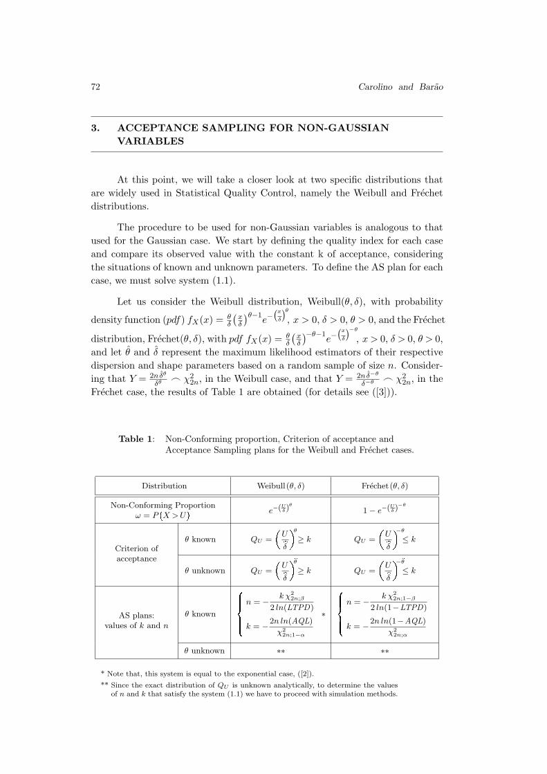
72 Carolino and Barao
3. ACCEPTANCE SAMPLING FOR NON-GAUSSIAN
VARIABLES
At this point, we will take a closer look at two specific distributions that
are widely used in Statistical Quality Control, namely the Weibull and Frechet
distributions.
The procedure to be used for non-Gaussian variables is analogous to that
used for the Gaussian case. We start by defining the quality index for each case
and compare its observed value with the constant k of acceptance, considering
the situations of known and unknown parameters. To define the AS plan for each
case, we must solve system (1.1).
Let us consider the Weibull distribution, Weibull(θ, δ), with probability
density function (pdf) fX(x) =θδ
(xδ
)θ−1e−
(x
δ
)θ
, x > 0, δ > 0, θ > 0, and the Frechet
distribution, Frechet(θ, δ), with pdf fX(x) =θδ
(xδ
)−θ−1e−
(x
δ
)−θ
, x > 0, δ > 0, θ > 0,
and let θ and δ represent the maximum likelihood estimators of their respective
dispersion and shape parameters based on a random sample of size n. Consider-
ing that Y =2nδθ
δθ ⌢ χ22n, in the Weibull case, and that Y =
2nδ−θ
δ−θ ⌢ χ22n, in the
Frechet case, the results of Table 1 are obtained (for details see ([3])).
Table 1: Non-Conforming proportion, Criterion of acceptance and
Acceptance Sampling plans for the Weibull and Frechet cases.
Distribution Weibull(θ, δ) Frechet(θ, δ)
Non-Conforming Proportione−(U
δ)θ
1 − e−(U
δ)−θ
ω = P�X > U
�Criterion ofacceptance
θ known QU =
�Ubδ �θ
≥ k QU =
�Ubδ �−θ
≤ k
θ unknown QU =
�Ubδ �bθ≥ k QU =
�Ubδ �−bθ
≤ k
AS plans:values of k and n
θ known
8>>><>>>: n = −
k χ22n;β
2 ln(LTPD)
k = −
2n ln(AQL)
χ22n;1−α
∗
8>>><>>>: n = −
k χ22n;1−β
2 ln(1−LTPD)
k = −
2n ln(1−AQL)
χ22n;α
θ unknown ∗∗ ∗∗
* Note that, this system is equal to the exponential case, ([2]).
** Since the exact distribution of QU is unknown analytically, to determine the valuesof n and k that satisfy the system (1.1) we have to proceed with simulation methods.
Robust Methods in AS 73
4. ROBUST ESTIMATORS FOR LOCATION
As we referred previously, when we have a non-Gaussian distribution we
can build specific AS plans associated with that distributions.
As also mentioned, the classical plans (Gaussian case) assume normality
of the data and they use X as an estimator of µ. However, when data is Non-
Gaussian, X may not be the best estimator, mainly when the distribution is
asymmetric and/or has heavy tails.
Thus, alternatively, as robust estimators for µ, we suggest the sample me-
dian(X
)and total median
(XT
), respectively, given by
X =
X(m) if n = 2m − 1 ,
Xm + Xm+1
2if n = 2m,
m ≥ 1 and XT =∑n
i=1 aiX(i), such that ai = an−i+1,∀ i = 1, ..., n, 0 < a1 < a2 <
... < a[
n2 ]
,∑n
i=1 ai = 1.
Considering these estimators for the mean value, the quality index of clas-
sical plans is, respectively Q′
N =U− eX
σ and Q′′
N =U− eXT
σ , and the criterion of ac-
ceptance, for each case is Q′
N =U− eX
σ ≥ k′
n and Q′′
N =U− eXT
σ ≥ k′′
n. When we work
with Q′
N , we use the distribution of X. When we work with Q′′
N , we need to use
simulation methods, since its distribution is unknown.
For calculating the weight of the tails, we used the index, τ ,([10]),
τ(F ) =1
2
(F−1
(0.99) − F−1(0.5)
F−1(0.75) − F−1(0.5)+
F−1(0.5) − F−1
(0.01)
F−1(0.5) − F−1(0.25)
)/(z0.99 − z0.5
z0.75 − z0.5
),
where F−1(p) represents the p-quantile of the distribution F and zp represents
de the p-quantile of the standard Gaussian distribution.
To assess the degree of skewness, Fisher’s skewness coefficient, c1, was used,
given by c1(F ) =µ3
σ3 , where F represents the distribution of the data, µ3 repre-
sents the third-order central moment of the distribution F and σ represents the
standard deviation of the distribution F .
According to ([7]), for asymmetric distributions, the best estimator for the
mean value is
• X, if c1 < 0.9 independently of the value of n or if n > 16 indepen-
dently of the value of c1;

74 Carolino and Barao
• XT , if 0.9 ≤ c1 ≤ 3.69 and n ≤ 16;
• X, if c1 > 3.69 and n = 3 or 4;
• XT , if c1 > 3.69 and 5 ≤ n ≤ 16.
For the tail weight index (τ), the best estimator for the mean value is
• X, if τ < 1.01 independently of the value of n;
• XT , if 1.01 ≤ τ ≤ 1.8 and n ≥ 5;
• X, if τ > 1.8 and n = 3 or 4;
• XT , if τ > 1.8 and n ≥ 5.
5. SOME RESULTS
Our main questions are: what miscalculations occur if X is Weibull and we
use a standard AS plan for Gaussian X instead? What alternatives can we use?
Can we use robust estimators for the location in the Gaussian case?
As we said before, the determination of the specific sampling plan is based
on the solution of the System (1.1). Usually α, β, AQL and LTPD are fixed
and the system is solved for n and k. For comparison of the plans it is more
convenient to fix n (taken from the standard) and solve the system to calculate
k and LTPD . The comparison of the results will, essentially, be based on LTPD
or/and the OC-curve.
To exemplify what we propose, we consider distributions with different
degrees of asymmetry and tail weight index. So we are going to compare the
Gaussian case with the Weibull (θ = 7 and θ = 1) and Frechet (θ = 5) cases.
We will consider α = 5%, β = 10%, AQL = 1% and several values of n, taken
from the standard.
5.1. Comparisons of Gaussian and specific plans
If the quality characteristic is a non-Gaussian variable and if we use the
values of the standard (apply the classical plans), the producers risk (5%) is
miscalculated and misleading. We have, therefore, to carry out the adjustment
of the α’s for the OC-curves which pass in the point (AQL, 1−α), and so we can
compare the sampling plans. For more details see ([3]). Table 2 shows the results
for the exponential case.
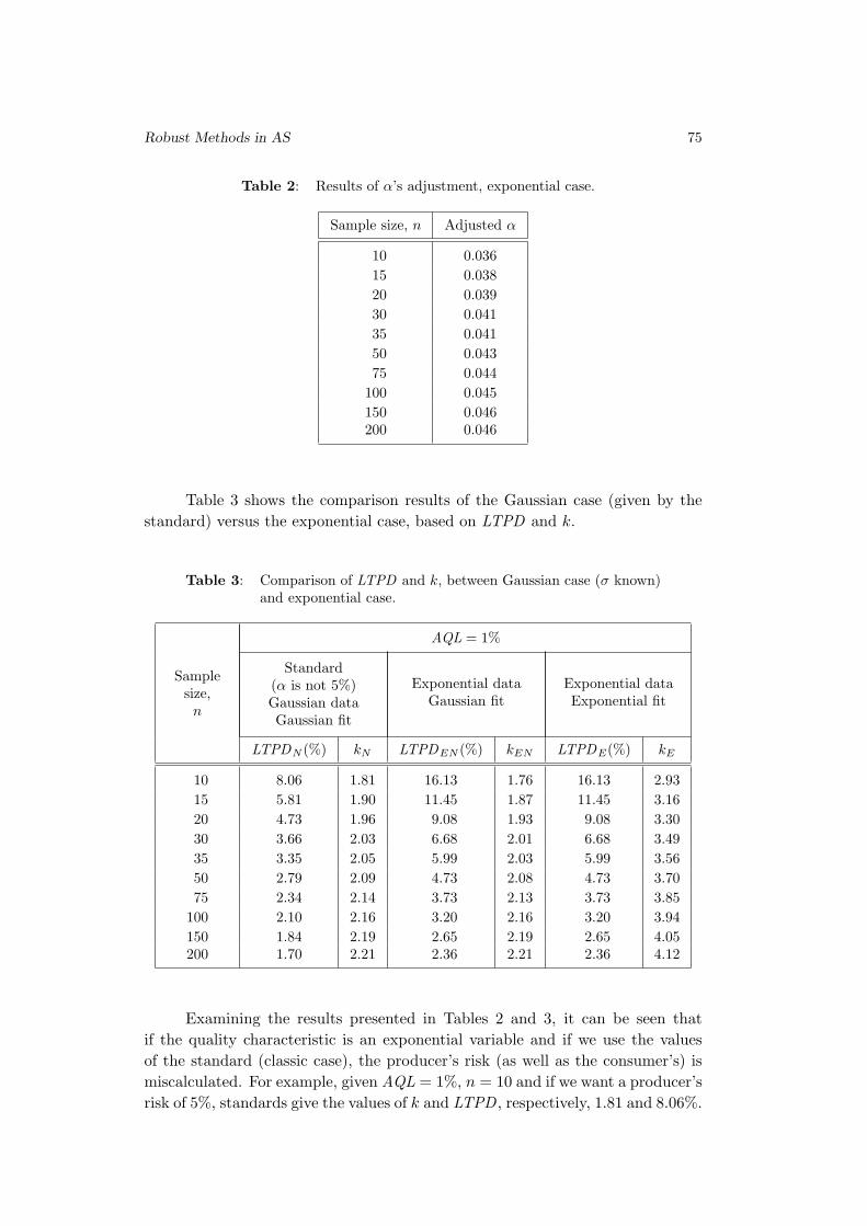
Robust Methods in AS 75
Table 2: Results of α’s adjustment, exponential case.
Sample size, n Adjusted α
10 0.036
15 0.038
20 0.039
30 0.041
35 0.041
50 0.043
75 0.044
100 0.045
150 0.046
200 0.046
Table 3 shows the comparison results of the Gaussian case (given by the
standard) versus the exponential case, based on LTPD and k.
Table 3: Comparison of LTPD and k, between Gaussian case (σ known)
and exponential case.
AQL = 1%
Sample
size,
n
Standard
(α is not 5%)
Gaussian data
Gaussian fit
Exponential data
Gaussian fit
Exponential data
Exponential fit
LTPDN (%) kN LTPDEN (%) kEN LTPDE(%) kE
10 8.06 1.81 16.13 1.76 16.13 2.93
15 5.81 1.90 11.45 1.87 11.45 3.16
20 4.73 1.96 9.08 1.93 9.08 3.30
30 3.66 2.03 6.68 2.01 6.68 3.49
35 3.35 2.05 5.99 2.03 5.99 3.56
50 2.79 2.09 4.73 2.08 4.73 3.70
75 2.34 2.14 3.73 2.13 3.73 3.85
100 2.10 2.16 3.20 2.16 3.20 3.94
150 1.84 2.19 2.65 2.19 2.65 4.05
200 1.70 2.21 2.36 2.21 2.36 4.12
Examining the results presented in Tables 2 and 3, it can be seen that
if the quality characteristic is an exponential variable and if we use the values
of the standard (classic case), the producer’s risk (as well as the consumer’s) is
miscalculated. For example, given AQL = 1%, n = 10 and if we want a producer’s
risk of 5%, standards give the values of k and LTPD , respectively, 1.81 and 8.06%.
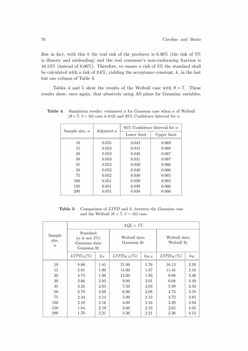
76 Carolino and Barao
But in fact, with this k the real risk of the producer is 6.36% (the risk of 5%
is illusory and misleading) and the real consumer’s non-conforming fraction is
16.13% (instead of 8.06%). Therefore, to ensure a risk of 5% the standard shall
be calculated with a risk of 3.6%, yielding the acceptance constant, k, in the last
but one column of Table 3.
Tables 4 and 5 show the results of the Weibull case with θ = 7. These
results show, once again, that abusively using AS plans for Gaussian variables,
Table 4: Simulation results: estimated α for Gaussian case when α of Weibull
(θ = 7, δ = 10) case is 0.05 and 95% Confidence Interval for α.
Sample size, n Adjusted α95% Confidence Interval for α
Lower limit Upper limit
10 0.055 0.042 0.069
15 0.053 0.041 0.068
20 0.053 0.040 0.067
30 0.053 0.041 0.067
35 0.052 0.039 0.066
50 0.052 0.040 0.066
75 0.052 0.040 0.065
100 0.051 0.039 0.065
150 0.051 0.039 0.066
200 0.051 0.038 0.066
Table 5: Comparison of LTPD and k, between the Gaussian case
and the Weibull (θ = 7, δ = 10) case.
AQL = 1%
Sample
size,
n
Standard
(α is not 5%)
Gaussian data
Gaussian fit
Weibull data
Gaussian fit
Weibull data
Weibull fit
LTPDN (%) kN LTPDWN (%) kWN LTPDW (%) kW
10 8.06 1.81 21.00 1.76 16.13 2.93
15 5.81 1.90 14.00 1.87 11.45 3.16
20 4.73 1.96 12.00 1.93 9.08 3.30
30 3.66 2.03 9.00 2.01 6.68 3.49
35 3.35 2.05 7.50 2.03 5.99 3.56
50 2.79 2.09 6.00 2.08 4.73 3.70
75 2.34 2.14 5.00 2.13 3.73 3.85
100 2.10 2.16 4.00 2.16 3.20 3.94
150 1.84 2.19 3.00 2.19 2.65 4.05
200 1.70 2.21 2.36 2.21 2.36 4.12
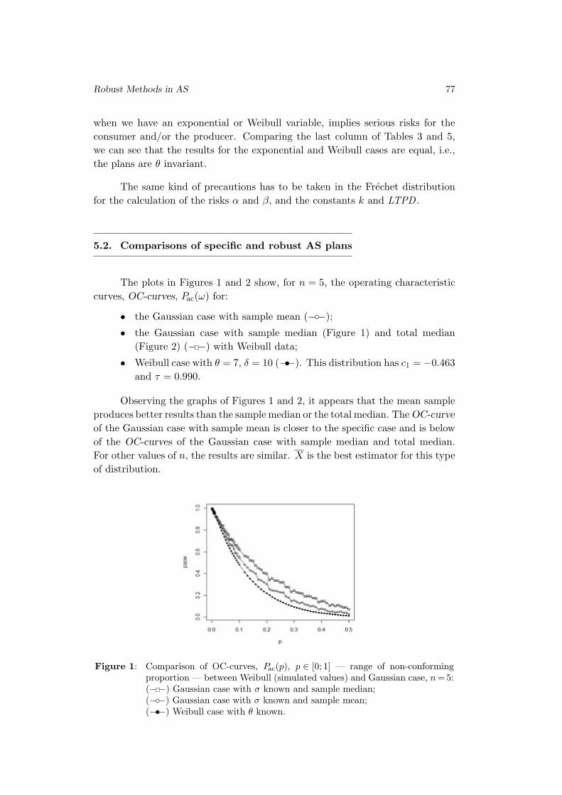
Robust Methods in AS 77
when we have an exponential or Weibull variable, implies serious risks for the
consumer and/or the producer. Comparing the last column of Tables 3 and 5,
we can see that the results for the exponential and Weibull cases are equal, i.e.,
the plans are θ invariant.
The same kind of precautions has to be taken in the Frechet distribution
for the calculation of the risks α and β, and the constants k and LTPD .
5.2. Comparisons of specific and robust AS plans
The plots in Figures 1 and 2 show, for n = 5, the operating characteristic
curves, OC-curves, Pac(ω) for:
• the Gaussian case with sample mean (−◦−);
• the Gaussian case with sample median (Figure 1) and total median
(Figure 2) (−�−) with Weibull data;
• Weibull case with θ = 7, δ = 10 (−•−). This distribution has c1 = −0.463
and τ = 0.990.
Observing the graphs of Figures 1 and 2, it appears that the mean sample
produces better results than the sample median or the total median. The OC-curve
of the Gaussian case with sample mean is closer to the specific case and is below
of the OC-curves of the Gaussian case with sample median and total median.
For other values of n, the results are similar. X is the best estimator for this type
of distribution.
Figure 1: Comparison of OC-curves, Pac(p), p ∈ [0; 1] — range of non-conforming
proportion — between Weibull (simulated values) and Gaussian case, n = 5:
(−�−) Gaussian case with σ known and sample median;
(−◦−) Gaussian case with σ known and sample mean;
(−•−) Weibull case with θ known.
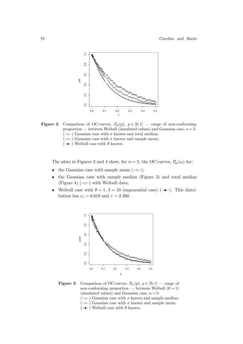
78 Carolino and Barao
Figure 2: Comparison of OC-curves, Pac(p), p ∈ [0; 1] — range of non-conforming
proportion — between Weibull (simulated values) and Gaussian case, n = 5:
(−�−) Gaussian case with σ known and total median;
(−◦−) Gaussian case with σ known and sample mean;
(−•−) Weibull case with θ known.
The plots in Figures 3 and 4 show, for n = 5, the OC-curves, Pac(ω) for:
• the Gaussian case with sample mean (−◦−);
• the Gaussian case with sample median (Figure 3) and total median
(Figure 4) (−�−) with Weibull data;
• Weibull case with θ = 1, δ = 10 (exponential case) (−•−). This distri-
bution has c1 = 6.619 and τ = 2.260.
Figure 3: Comparison of OC-curves, Pac(p), p ∈ [0; 1] — range of
non-conforming proportion — between Weibull (θ = 1)
(simulated values) and Gaussian case, n = 5:
(−�−) Gaussian case with σ known and sample median;
(−◦−) Gaussian case with σ known and sample mean;
(−•−) Weibull case with θ known.
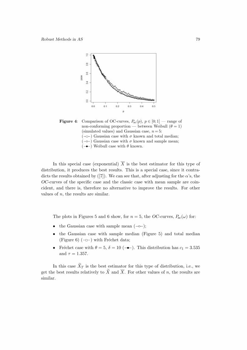
Robust Methods in AS 79
Figure 4: Comparison of OC-curves, Pac(p), p ∈ [0; 1] — range of
non-conforming proportion — between Weibull (θ = 1)
(simulated values) and Gaussian case, n = 5:
(−�−) Gaussian case with σ known and total median;
(−◦−) Gaussian case with σ known and sample mean;
(−•−) Weibull case with θ known.
In this special case (exponential) X is the best estimator for this type of
distribution, it produces the best results. This is a special case, since it contra-
dicts the results obtained by ([7]). We can see that, after adjusting for the α’s, the
OC-curves of the specific case and the classic case with mean sample are coin-
cident, and there is, therefore no alternative to improve the results. For other
values of n, the results are similar.
The plots in Figures 5 and 6 show, for n = 5, the OC-curves, Pac(ω) for:
• the Gaussian case with sample mean (−◦−);
• the Gaussian case with sample median (Figure 5) and total median
(Figure 6) (−�−) with Frechet data;
• Frechet case with θ = 5, δ = 10 (−•−). This distribution has c1 = 3.535
and τ = 1.357.
In this case XT is the best estimator for this type of distribution, i.e., we
get the best results relatively to X and X. For other values of n, the results are
similar.
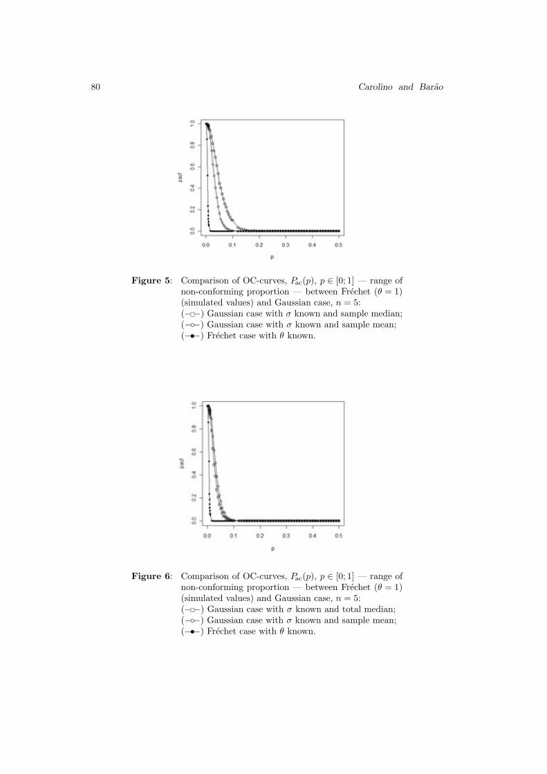
80 Carolino and Barao
Figure 5: Comparison of OC-curves, Pac(p), p ∈ [0; 1] — range of
non-conforming proportion — between Frechet (θ = 1)
(simulated values) and Gaussian case, n = 5:
(−�−) Gaussian case with σ known and sample median;
(−◦−) Gaussian case with σ known and sample mean;
(−•−) Frechet case with θ known.
Figure 6: Comparison of OC-curves, Pac(p), p ∈ [0; 1] — range of
non-conforming proportion — between Frechet (θ = 1)
(simulated values) and Gaussian case, n = 5:
(−�−) Gaussian case with σ known and total median;
(−◦−) Gaussian case with σ known and sample mean;
(−•−) Frechet case with θ known.
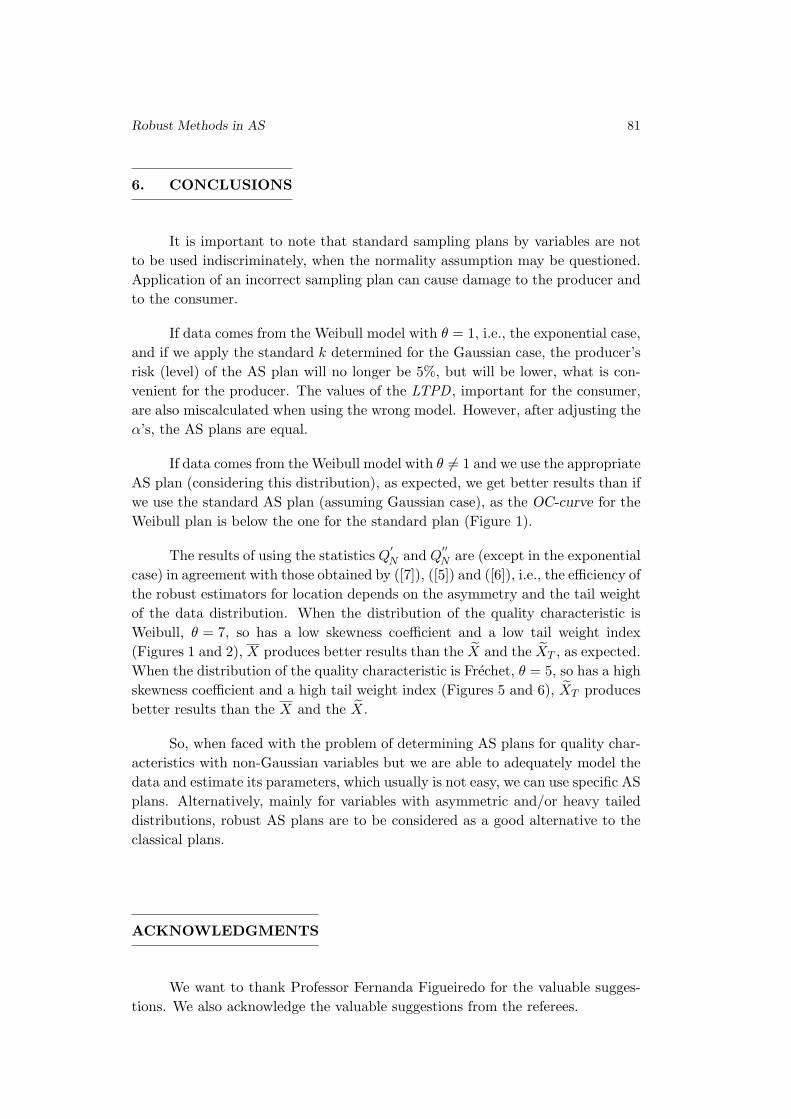
Robust Methods in AS 81
6. CONCLUSIONS
It is important to note that standard sampling plans by variables are not
to be used indiscriminately, when the normality assumption may be questioned.
Application of an incorrect sampling plan can cause damage to the producer and
to the consumer.
If data comes from the Weibull model with θ = 1, i.e., the exponential case,
and if we apply the standard k determined for the Gaussian case, the producer’s
risk (level) of the AS plan will no longer be 5%, but will be lower, what is con-
venient for the producer. The values of the LTPD , important for the consumer,
are also miscalculated when using the wrong model. However, after adjusting the
α’s, the AS plans are equal.
If data comes from the Weibull model with θ 6= 1 and we use the appropriate
AS plan (considering this distribution), as expected, we get better results than if
we use the standard AS plan (assuming Gaussian case), as the OC-curve for the
Weibull plan is below the one for the standard plan (Figure 1).
The results of using the statistics Q′
N and Q′′
N are (except in the exponential
case) in agreement with those obtained by ([7]), ([5]) and ([6]), i.e., the efficiency of
the robust estimators for location depends on the asymmetry and the tail weight
of the data distribution. When the distribution of the quality characteristic is
Weibull, θ = 7, so has a low skewness coefficient and a low tail weight index
(Figures 1 and 2), X produces better results than the X and the XT , as expected.
When the distribution of the quality characteristic is Frechet, θ = 5, so has a high
skewness coefficient and a high tail weight index (Figures 5 and 6), XT produces
better results than the X and the X.
So, when faced with the problem of determining AS plans for quality char-
acteristics with non-Gaussian variables but we are able to adequately model the
data and estimate its parameters, which usually is not easy, we can use specific AS
plans. Alternatively, mainly for variables with asymmetric and/or heavy tailed
distributions, robust AS plans are to be considered as a good alternative to the
classical plans.
ACKNOWLEDGMENTS
We want to thank Professor Fernanda Figueiredo for the valuable sugges-
tions. We also acknowledge the valuable suggestions from the referees.

82 Carolino and Barao
REFERENCES
[1] ANSI/ASQC Z1.9-2011 (2011). Sampling Procedures and Tables for Inspection
by Variables for Percent Nonconforming, ASQ, Milwaukee, WI (USA).
[2] Carolino, E.; Casquilho, M. and Barao, M. (2007). Amostragem de
aceitacao para uma variavel assimetrica: a Exponencial, Actas do XIV Congresso
Anual da Sociedade Portuguesa de Estatıstica, 281–292.
[3] Carolino, Elisabete (2012). Amostragem de Aceitacao para Variaveis nao
Gaussianas, PhD Dissertation (in portuguese), FCUL, Portugal.
[4] Duncan, A.J. (1986). Quality Control and Industrial Statistics, 5th
edition,
IRWIN, USA.
[5] Figueiredo, F. and Gomes, M.I. (2004). The total median in statistical quality
control, Applied stochastic models in business and industry, 20, 339–353.
[6] Figueiredo, F. and Gomes, M.I. (2009). Monitoring industrial processes with
robust control charts, Revstat, 7, 151–170.
[7] Figueiredo, F.O. (2003). Controlo Estatıstico da Qualidade e Metodos Robus-
tos, PhD Dissertation (in portuguese), FCUL, Portugal.
[8] Gomes, M.I.; Figueiredo, F. and Barao, M.I. (2010). Controlo Estatıstico
da Qualidade, Segunda Edicao revista e aumentada, Edicoes SPE.
[9] Guenther, William C. (1977). Sampling Inspection in Statistical Quality Con-
trol, First published, Whitstable Litho Ltd, GB.
[10] Hoaglin, David C.; Mosteller, Frederick and Tuckey, John W. (2000).
Understanding Robust and Explanatory Data Analysis, John Wiley and Sons, Inc.,
New York.
[11] Levinson, W. (1997). Watch out for non-normal distributions of impurities,
Chemical Engineering Progress, 70–76.
[12] Montgomery, D.C. (2004). Introduction to Statistical Quality Control, 5th
edi-
tion, John Wiley and Sons, Inc., New York, USA.
[13] Schilling, E.G. and Neubauer, D.V. (2009). Acceptance sampling in Quality
Control, 2nd
ed., Chapman and Hall / CRC, New York, USA.
[14] Wetherill, G.B. and Brown, D.W. (1991). Statistical Process Control, Chap-
man and Hall, London, UK.
REVSTAT – Statistical Journal
Volume 11, Number 1, March 2013, 83–104
THE SKEW-NORMAL DISTRIBUTION IN SPC
Authors: Fernanda Figueiredo
– CEAUL and Faculdade de Economia da Universidade do Porto, Portugal
M. Ivette Gomes
– Universidade de Lisboa, FCUL, DEIO and CEAUL, Portugal
Abstract:
• Modeling real data sets, even when we have some potential (as)symmetric models for
the underlying data distribution, is always a very difficult task due to some uncon-
trollable perturbation factors. The analysis of different data sets from diverse areas
of application, and in particular from statistical process control (SPC), leads us to
notice that they usually exhibit moderate to strong asymmetry as well as light to
heavy tails, which leads us to conclude that in most of the cases, fitting a normal
distribution to the data is not the best option, despite of the simplicity and popu-
larity of the Gaussian distribution. In this paper we consider a class of skew-normal
models that include the normal distribution as a particular member. Some properties
of the distributions belonging to this class are enhanced in order to motivate their use
in applications. To monitor industrial processes some control charts for skew-normal
and bivariate normal processes are developed, and their performance analyzed. An
application with a real data set from a cork stopper’s process production is presented.
Key-Words:
• bootstrap control charts; false alarm rate; heavy-tails; Monte Carlo simulations;
probability limits; run-length; shewhart control charts; skewness; skew-normal dis-
tribution; statistical process control.
AMS Subject Classification:
• 62G05, 62G35, 62P30, 65C05.

84 Fernanda Figueiredo and M. Ivette Gomes
The Skew-Normal Distribution in SPC 85
1. INTRODUCTION
The most commonly used standard procedures of statistical quality control
(SQC), control charts and acceptance sampling plans, are often implemented un-
der the assumption of normal data, which rarely holds in practice. The analysis
of several data sets from diverse areas of application, such as, statistical process
control (SPC), reliability, telecommunications, environment, climatology and fi-
nance, among others, leads us to notice that this type of data usually exhibit
moderate to strong asymmetry as well as light to heavy tails. Thus, despite
of the simplicity and popularity of the Gaussian distribution, we conclude that
in most of the cases, fitting a normal distribution to the data is not the best
option. On the other side, modeling real data sets, even when we have some
potential (as)symmetric models for the underlying data distribution, is always a
very difficult task due to some uncontrollable perturbation factors.
This paper focus on the parametric family of skew-normal distributions
introduced by O’Hagan and Leonard (1976), and investigated with more detail
by Azzalini (1985, 1986, 2005), among others.
Definition 1.1. A random variable (rv) Y is said to have a location-scale
skew-normal distribution, with location at λ, scale at δ and shape parameter α,
and we denote Y ∼ SN(λ, δ2, α), if its probability density function (pdf) is given
by
(1.1) f(y; λ, δ, α) =2
δφ
(y −λ
δ
)Φ
(α
y −λ
δ
), y ∈R (α, λ∈R, δ ∈R
+) ,
where φ and Φ denote, as usual, the pdf and the cumulative distribution function
(cdf) of the standard normal distribution, respectively. If λ = 0 and δ = 1, we
obtain the standard skew-normal distribution, denoted by SN(α).
This class of distributions includes models with different levels of skewness
and kurtosis, apart from the normal distribution itself (α = 0). In this sense, it
can be considered an extension of the normal family. Allowing departures from
the normal model, by the introduction of the extra parameter α that controls the
skewness, its use in applications will provide more robustness in inferential meth-
ods, and perhaps better models to fit the data, for instance, when the empirical
distribution has a shape similar to the normal, but exhibits a slight asymmetry.
Note that even in potential normal situations there is some possibility of hav-
ing disturbances in the data, and the skew-normal family of distributions can
describe the process data in a more reliable and robust way. In applications it
is also important to have the possibility of regulating the thickness of the tails,
apart of the skewness.
86 Fernanda Figueiredo and M. Ivette Gomes
The cdf of the skew-normal rv Y defined in (1.1) is given by
(1.2) F (y; λ, δ, α) = Φ
(y −λ
δ
)−2 T
(y −λ
δ, α
), y ∈R (α, λ∈R, δ ∈R
+) ,
where T (h, b) is the Owen’s T function (integral of the standard normal bivariate
density, bounded by x = h, y = 0 and y = b x), tabulated in Owen (1956), and
that can be defined by T (h, b) =1
2π
∫ b
0
{e−
12 h2(1+x2)/(1+ x2
)
}dx, (b, h) ∈ R×R.
Although the pdf in (1.1) has a very simple expression the same does not
happen with the cdf in (1.2), but this is not a problem that leads us to avoid
the use of the skew-normal distribution. We have access to the R package ‘sn’
(version 0.4-17) developed by Azzalini (2011), for instance, that provides func-
tions related to the skew-normal distribution, including the density function, the
distribution function, the quantile function, random number generators and max-
imum likelihood estimates. The moment generating function of the rv Y is given
by MY (t) = 2 exp(λt + δ2t2/2
)Φ(θδ t), ∀ t ∈ R, where θ = α/
√1 + α2 ∈ (−1, 1),
and there exist finite moments of all orders.
Other classes of skew normal distributions, for the univariate and the mul-
tivariate case, together with the related classes of skew-t distributions, have been
recently revisited and studied in the literature. For details see Fernandez and
Steel (1998), Abtahi et al. (2011) and Jamalizadeb et al. (2011), among others.
In this paper some control charts based on the skew-normal distribution are pro-
posed. They still are parametric control charts, and should be compared with
the so-called nonparametric or distribution-free control charts that require even
less restrictive assumptions, a topic out of the scope of this paper. We merely
mention that the nonparametric charts have the same in-control run-length dis-
tribution for every continuous distribution, and thus, are by definition robust. In
the literature several Shewhart, CUSUM and EWMA type nonparametric control
charts have been proposed. Most of them are devised to monitor the location and
are based on well-known nonparametric test statistics. For a recent overview on
the latest developments on nonparametric control charts, see Chakraborti et al.
(2011) and references therein.
This paper is organized as follows. Section 2 provides some information
about the family of skew-normal distributions, in what concerns properties, ran-
dom sample generation and inference. Section 3 presents bootstrap control charts
for skew-normal processes and some simulation results about their performance.
Control charts based on specific statistics with a skew normal distribution are
considered to monitor bivariate normal processes, and their properties evaluated.
In Section 4, an application in the field of SQC is provided. The paper ends with
some conclusions and recommendations in Section 5.
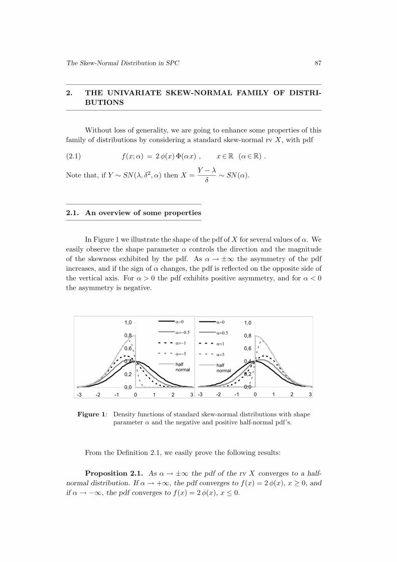
The Skew-Normal Distribution in SPC 87
2. THE UNIVARIATE SKEW-NORMAL FAMILY OF DISTRI-
BUTIONS
Without loss of generality, we are going to enhance some properties of this
family of distributions by considering a standard skew-normal rv X, with pdf
(2.1) f(x; α) = 2φ(x) Φ(αx) , x∈R (α∈R) .
Note that, if Y ∼ SN(λ, δ2, α) then X =Y − λ
δ∼ SN(α).
2.1. An overview of some properties
In Figure 1 we illustrate the shape of the pdf of X for several values of α. We
easily observe the shape parameter α controls the direction and the magnitude
of the skewness exhibited by the pdf. As α → ±∞ the asymmetry of the pdf
increases, and if the sign of α changes, the pdf is reflected on the opposite side of
the vertical axis. For α > 0 the pdf exhibits positive asymmetry, and for α < 0
the asymmetry is negative.
0,0
0,2
0,4
0,6
0,8
1,0
-3 -2 -1 0 1 2 3
half
normal
0,0
0,2
0,4
0,6
0,8
1,0
-3 -2 -1 0 1 2 3
half
normal
Figure 1: Density functions of standard skew-normal distributions with shape
parameter α and the negative and positive half-normal pdf’s.
From the Definition 2.1, we easily prove the following results:
Proposition 2.1. As α → ±∞ the pdf of the rv X converges to a half-
normal distribution. If α → +∞, the pdf converges to f(x) = 2φ(x), x ≥ 0, and
if α → −∞, the pdf converges to f(x) = 2φ(x), x ≤ 0.

88 Fernanda Figueiredo and M. Ivette Gomes
Proposition 2.2. If X ∼ SN(α) then the rv W = |X| has a half-normal
distribution with pdf given by f(w) = 2φ(w), w ≥ 0, and the rv T = X2, the
square of a half-normal distribution, has a pdf given by f(t) =1√2π
t−1/2 e−t2/2,
t ≥ 0, i.e., has a chi-square distribution with 1 degree of freedom.
Denoting the usual sign function by sign(·) and taking θ = α/√
1 + α2, the
rv X with a standard skew-normal distribution SN(α) has mean value given by
E(X) =
√2
πθ −→
α→±∞sign(α) × 0.79788 ,
and variance equal to
V(X) = 1 − 2
πθ2 −→
α→±∞0.36338 .
The Fisher coefficient of skewness is given by
β1 =(4 − π)
√2 θ6/π3
√−8θ6/π3 + 12 θ4/π2 − 6θ2/π + 1
−→α→±∞
sign(α) × 0.99527 .
From these expressions we easily observe that the mean value and the de-
gree of skewness of the SN(α) distribution increases with |α| while the variance
decreases, but they all converge to a finite value.
Taking into consideration the large asymmetry of the SN(α) distribution
when α → ±∞, and the fact that the kurtosis coefficient expresses a balanced
weight of the two-tails, we shall here evaluate separately the right-tail weight and
the left-tail weight of the SN(α) distribution through the coefficients τR and τL
defined by
τR :=
(F−1
(0.99) − F−1(0.5)
F−1(0.75) − F−1(0.5)
)(Φ−1
(0.99) − Φ−1
(0.5)
Φ−1(0.75) − Φ−1(0.5)
)−1
and
τL :=
(F−1
(0.5) − F−1(0.01)
F−1(0.5) − F−1(0.25)
)(Φ−1
(0.5) − Φ−1
(0.01)
Φ−1(0.5) − Φ−1(0.25)
)−1
,
where F−1and Φ
−1denote the inverse functions of the cdf of the SN(α) and of
the cdf of the standard normal distributions, respectively. These coefficients are
based on the tail-weight coefficient τ defined in Hoaglin et al. (1983) for symmetric
distributions. For the normal distribution, τL = τR = 1. If the distribution F has
a right (left) tail heavier than the normal tails, τR > 1 (τL > 1), and if F has a
right (left) tail thinner than the normal tails, τR < 1 (τL < 1).
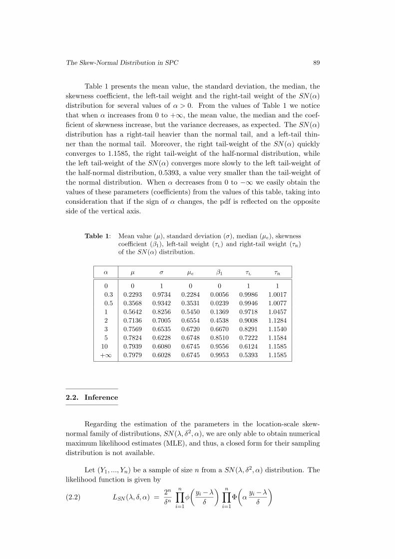
The Skew-Normal Distribution in SPC 89
Table 1 presents the mean value, the standard deviation, the median, the
skewness coefficient, the left-tail weight and the right-tail weight of the SN(α)
distribution for several values of α > 0. From the values of Table 1 we notice
that when α increases from 0 to +∞, the mean value, the median and the coef-
ficient of skewness increase, but the variance decreases, as expected. The SN(α)
distribution has a right-tail heavier than the normal tail, and a left-tail thin-
ner than the normal tail. Moreover, the right tail-weight of the SN(α) quickly
converges to 1.1585, the right tail-weight of the half-normal distribution, while
the left tail-weight of the SN(α) converges more slowly to the left tail-weight of
the half-normal distribution, 0.5393, a value very smaller than the tail-weight of
the normal distribution. When α decreases from 0 to −∞ we easily obtain the
values of these parameters (coefficients) from the values of this table, taking into
consideration that if the sign of α changes, the pdf is reflected on the opposite
side of the vertical axis.
Table 1: Mean value (µ), standard deviation (σ), median (µe), skewness
coefficient (β1), left-tail weight (τL) and right-tail weight (τR)
of the SN(α) distribution.
α µ σ µe β1 τL τR
0 0 1 0 0 1 1
0.3 0.2293 0.9734 0.2284 0.0056 0.9986 1.0017
0.5 0.3568 0.9342 0.3531 0.0239 0.9946 1.0077
1 0.5642 0.8256 0.5450 0.1369 0.9718 1.0457
2 0.7136 0.7005 0.6554 0.4538 0.9008 1.1284
3 0.7569 0.6535 0.6720 0.6670 0.8291 1.1540
5 0.7824 0.6228 0.6748 0.8510 0.7222 1.1584
10 0.7939 0.6080 0.6745 0.9556 0.6124 1.1585
+∞ 0.7979 0.6028 0.6745 0.9953 0.5393 1.1585
2.2. Inference
Regarding the estimation of the parameters in the location-scale skew-
normal family of distributions, SN(λ, δ2, α), we are only able to obtain numerical
maximum likelihood estimates (MLE), and thus, a closed form for their sampling
distribution is not available.
Let (Y1, ..., Yn) be a sample of size n from a SN(λ, δ2, α) distribution. The
likelihood function is given by
(2.2) LSN (λ, δ, α) =2
n
δn
n∏
i=1
φ
(yi −λ
δ
) n∏
i=1
Φ
(α
yi −λ
δ
)
90 Fernanda Figueiredo and M. Ivette Gomes
and the log-likelihood is given by
ln LSN (λ, δ, α) = n ln 2 − n ln δ +
n∑
i=1
lnφ
(yi −λ
δ
)+
n∑
i=1
ln Φ
(α
yi −λ
δ
),
where ln(·) denotes the natural logarithm function.
The MLE estimates of λ, δ and α, denoted λ, δ and α, are the numerical
solution of the system of equations
(2.3)
δ2=
1
n
n∑
i=1
(yi −λ)2 ,
αn∑
i=1
φ(α yi−λ
δ
)
Φ
(α yi−λ
δ
) =
n∑
i=1
yi −λ
δ,
n∑
i=1
yi−λδ φ
(αyi−λ
δ
)
Φ
(α yi−λ
δ
) = 0 .
We may have some problems to obtain these estimates in the case of small-
to-moderate values of the sample size n as well as for values of α close to zero.
Note that if all the values of the sample are positive (negative), for fixed values
of λ and δ, the log-likelihood function is an increasing (decreasing) function of α,
producing therefore boundary estimates, and for α = 0, the expected Fisher
information matrix is singular.
Several authors have given important suggestions to find these estimates.
For instance, for a fixed value of α, solve the last two equations of (2.3) for
obtaining λ and δ, taking into account the first equation, and then, repeat these
steps for a reasonable range of values of α. Another suggestion to get around
these problems of estimation is to consider another re-parametrization for the
skew-normal distributions SN(λ, δ2, α) in (1.1), in terms of the mean value µ, the
standard deviation σ and the asymmetry coefficient β1. For details in this topic
see, for instance, Azzalini (1985), Azzalini and Capitanio (1999) and Azzalini and
Regoli (2012), among others.
To decide between the use of a normal or a skew-normal distribution to fit
the data, apart from the information given by the histogram associated to the
data sample and the fitted pdf estimated by maximum likelihood, we can advance
to the confirmatory phase with a likelihood ratio test.
To test the normal distribution against a skew-normal distribution, i.e.,
the hypotheses H0 : X ∼ SN(λ, δ2, α = 0) versus H1 : X ∼ SN(λ, δ2, α 6= 0), the
The Skew-Normal Distribution in SPC 91
likelihood ratio statistic Λ is given by
(2.4) Λ =LSN
(λ, δ, α = 0)
LSN
(λ, δ, α
) ,
where LSN(λ,δ,α), given in (2.2), denotes the likelihood function for the SN(λ,δ2,α)
distribution. Under the null hypothesis, −2 logΛ is distributed as a chi-square
distribution with 1 degree of freedom. For a large observed value of −2 logΛ, we
reject the null hypothesis, i.e., there is a strong evidence that the SN(λ, δ2, α
)
distribution presents a better fit than the normal N(µ, σ2) distribution to the
data set under consideration.
2.3. Other stochastic results
Among other results valid for the skew-normal distribution, we shall refer
the following ones:
Proposition 2.3. If Z1 and Z2 are independent random variables with
standard normal distribution, then Z1|Z2≤αZ1 ∼ SN (α). Also,
X :=
{Z2 if Z1 < αZ2
−Z2 otherwise∼ SN(α) .
Proposition 2.3 allows us to write the following algorithm for the generation
of random samples, (Y1, ..., Yn), of size n, from a SN(λ, δ2, α) distribution.
Algorithm 2.1. Repeat Steps 1.–4. for i = 1 to n:
1. Generate two independent values, Z1 and Z2, from a N(0,1) distribution;
2. Compute T = α Z2;
3. The value Xi =
{Z2 if Z1 < T
−Z2 otherwisecomes from a SN(α);
4. The value Yi = λ + δXi comes from a SN(λ, δ2, α).
Figure 2 presents four histograms associated to samples of size one thou-
sand generated from a SN(α) distribution with shape parameter α = 0, 1, 2, 3,
respectively, together with the pdf’s of a normal and of a skew normal distribu-
tion fitted to the data by maximum likelihood. From Figure 2 we easily observe
that as α increases the differences between the two estimated pdf’s become larger,
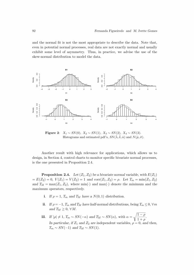
92 Fernanda Figueiredo and M. Ivette Gomes
and the normal fit is not the most appropriate to describe the data. Note that,
even in potential normal processes, real data are not exactly normal and usually
exhibit some level of asymmetry. Thus, in practice, we advise the use of the
skew-normal distribution to model the data.
X1
X1
Density
!4 !3 !2 !1 0 1 2 3
0.0
0.2
0.4
X2
X2
Density
!2 !1 0 1 2 3 4
0.0
0.2
0.4
X3
X3
Density
!1 0 1 2 3 4
0.0
0.2
0.4
0.6
X4
X4
Density
!1 0 1 2 3 4
0.0
0.2
0.4
0.6
Figure 2: X1 ∼ SN(0), X2 ∼ SN(1), X3 ∼ SN(2), X4 ∼ SN(3).
Histograms and estimated pdf’s, SN(λ, δ, α) and N(µ, σ).
Another result with high relevance for applications, which allows us to
design, in Section 4, control charts to monitor specific bivariate normal processes,
is the one presented in Proposition 2.4.
Proposition 2.4. Let (Z1, Z2) be a bivariate normal variable, with E(Z1)
= E(Z2) = 0, V (Z1) = V (Z2) = 1 and corr(Z1, Z2) = ρ. Let Tm = min(Z1, Z2)
and TM = max(Z1, Z2), where min(·) and max(·) denote the minimum and the
maximum operators, respectively.
i. If ρ = 1, Tm and TM have a N(0, 1) distribution.
ii. If ρ =−1, Tm and TM have half-normal distributions, being Tm ≤ 0, ∀m
and TM ≥ 0, ∀M.
iii. If |ρ| 6= 1, Tm ∼ SN(−α) and TM ∼ SN(α), with α =
√1 − ρ
1 + ρ.
In particular, if Z1 and Z2 are independent variables, ρ = 0, and then,
Tm ∼ SN(−1) and TM ∼ SN(1).

The Skew-Normal Distribution in SPC 93
3. CONTROL CHARTS BASED ON THE SKEW-NORMAL DIS-
TRIBUTION
The most commonly used charts for monitoring industrial processes, or
more precisely, a quality characteristic X at the targets µ0 and σ0, the desired
mean value and standard deviation of X, respectively, are the Shewhart con-
trol charts with 3-sigma control limits. More precisely, the sample mean chart
(M -chart), the sample standard deviation chart (S-chart) and the sample range
chart (R-chart), which are usually developed under the assumptions of indepen-
dent and normally distributed data. Additionally, the target values µ0 and σ0 are
not usually fixed given values, and we have to estimate them, in order to obtain
the control limits of the chart.
The ability of a control chart to detect process changes is usually measured
by the expected number of samples taken before the chart signals, i.e., by its
ARL (average run length), together with the standard deviation of the run length
distribution, SDRL.
Whenever implementing a control chart, a practical advice is that 3-sigma
control limits should be avoided whenever the distribution of the control statistic
is very asymmetric. In such a case, it is preferable to fix the control limits of
the chart at adequate probability quantiles of the control statistic distribution, in
order to obtain a fixed ARL when the process is in-control, usually 200, 370.4, 500
or 1000, or equivalently, the desired FAR (false alarm rate), i.e., the probability
that an observation is considered as out-of-control when the process is actually
in-control, usually 0.005, 0.0027, 0.002 or 0.001. General details about Shewhart
control charts can be found, for instance, in Montgomery (2005).
In the case of skew-normal processes we do not have explicit formulas for
the MLE estimators of the location, scale and shape parameters, and thus, a
closed-form for their sampling distribution is not available. The same happens
for other statistics of interest, such as, the sample mean, the sample standard
deviation, the sample range and the sample percentiles, among others. Thus,
to monitor skew-normal processes, the bootstrap control charts are very useful,
despite of the disadvantages of a highly time-consuming Phase I. Moreover, many
papers, see for instance, Seppala et al. (1995), Liu and Tang (1996) and Jones
and Woodall (1998), refer that for skewed distributions, bootstrap control charts
have on average a better performance than the Shewhart control charts. Other
details about the bootstrap methodology and bootstrap control charts can be
found, for instance, in Efron and Tibshirani (1993), Bai and Choi (1995), Nichols
and Padgett (2006) and Lio and Park (2008, 2010).
94 Fernanda Figueiredo and M. Ivette Gomes
3.1. Bootstrap control charts for skew-normal processes
To construct a bootstrap control chart we only use the sample data to
estimate the sampling distribution of the parameter estimator, and then, to ob-
tain appropriate control limits. Thus, only the usual assumptions of Phase II
of SPC are required: stable process and independent and identically distributed
subgroup observations. The following Algorithm 3.1, similar to the ones proposed
in Nichols and Padgett (2006) and Lio and Park (2008, 2010), can be used to im-
plement bootstrap control charts for subgroup samples of size n, to monitor the
process mean value and the process standard deviation of a skew-normal distri-
bution, respectively. This algorithm can be easily modified in order to implement
bootstrap control charts for other parameters of interest.
Algorithm 3.1.
Phase I: Estimation and computation of the control limits
1. From in-control and stable process, observe k, say 25 or 30, random
samples of size n, assuming the observations are independent and come
from a skew-normal distribution, SN(λ, δ2, α).
2. Compute the MLE estimates of λ, δ and α, using the pooled sample of
size k×n.
3. Generate a parametric bootstrap sample of size n, (x∗1, ..., x
∗n), from a
skew-normal distribution and using the MLEs obtained in Step 2. as
the distribution parameters.
4. Select the Step associated to the chart you want to implement:
i. Two-sided bootstrap M-chart to monitor the process mean
value µ: from the bootstrap subgroup sample obtained in Step 3.,
compute the sample mean, µ∗= x∗
.
ii. Upper one-sided bootstrap S-chart to monitor the process
standard deviation σ: from the bootstrap subgroup sample ob-
tained in Step 3., compute the sample standard deviation, σ∗= s∗.
5. Repeat Steps 3.–4., a large number of times, say B = 10 000 times,
obtaining B bootstrap estimates of the parameter of interest, in our
case, the process mean value or the standard deviation.
6. Let γ be the desired false alarm rate (FAR) of the chart. Using the B
bootstrap estimates obtained in Step 5.,
i. Find the 100(γ/2)th and 100(1−γ/2)th quantiles of the distribu-
tion of µ∗, i.e., the lower control limit LCL and the upper control
limit UCL for the bootstrap M -chart of FAR=γ, respectively.
ii. Find the 100(1−γ)th quantile of the distribution of σ∗, i.e., the
upper control limit UCL for the bootstrap S-chart of FAR=γ. The
lower control limit LCL is placed at 0.
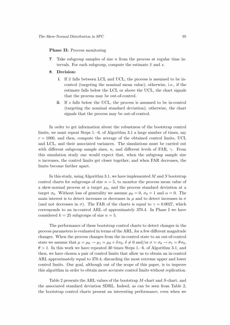
The Skew-Normal Distribution in SPC 95
Phase II: Process monitoring
7. Take subgroup samples of size n from the process at regular time in-
tervals. For each subgroup, compute the estimate x and s.
8. Decision:
i. If x falls between LCL and UCL, the process is assumed to be in-
control (targeting the nominal mean value); otherwise, i.e., if the
estimate falls below the LCL or above the UCL, the chart signals
that the process may be out-of-control.
ii. If s falls below the UCL, the process is assumed to be in-control
(targeting the nominal standard deviation); otherwise, the chart
signals that the process may be out-of-control.
In order to get information about the robustness of the bootstrap control
limits, we must repeat Steps 1.–6. of Algorithm 3.1 a large number of times, say
r = 1000, and then, compute the average of the obtained control limits, UCL
and LCL, and their associated variances. The simulations must be carried out
with different subgroup sample sizes, n, and different levels of FAR, γ. From
this simulation study one would expect that, when the subgroup sample size
n increases, the control limits get closer together, and when FAR decreases, the
limits become farther apart.
In this study, using Algorithm 3.1, we have implemented M and S bootstrap
control charts for subgroups of size n = 5, to monitor the process mean value of
a skew-normal process at a target µ0, and the process standard deviation at a
target σ0. Without loss of generality we assume µ0 = 0, σ0 = 1 and α = 0. The
main interest is to detect increases or decreases in µ and to detect increases in σ
(and not decreases in σ). The FAR of the charts is equal to γ = 0.0027, which
corresponds to an in-control ARL of approximately 370.4. In Phase I we have
considered k = 25 subgroups of size n = 5.
The performance of these bootstrap control charts to detect changes in the
process parameters is evaluated in terms of the ARL, for a few different magnitude
changes. When the process changes from the in-control state to an out-of-control
state we assume that µ = µ0 → µ1 = µ0 + δσ0, δ 6= 0 and/or σ = σ0 → σ1 = θσ0,
θ > 1. In this work we have repeated 30 times Steps 1.–6. of Algorithm 3.1, and
then, we have chosen a pair of control limits that allow us to obtain an in-control
ARL approximately equal to 370.4, discarding the most extreme upper and lower
control limits. Our goal, although out of the scope of this paper, is to improve
this algorithm in order to obtain more accurate control limits without replication.
Table 2 presents the ARL values of the bootstrap M -chart and S-chart, and
the associated standard deviation SDRL. Indeed, as can be seen from Table 2,
the bootstrap control charts present an interesting performance, even when we
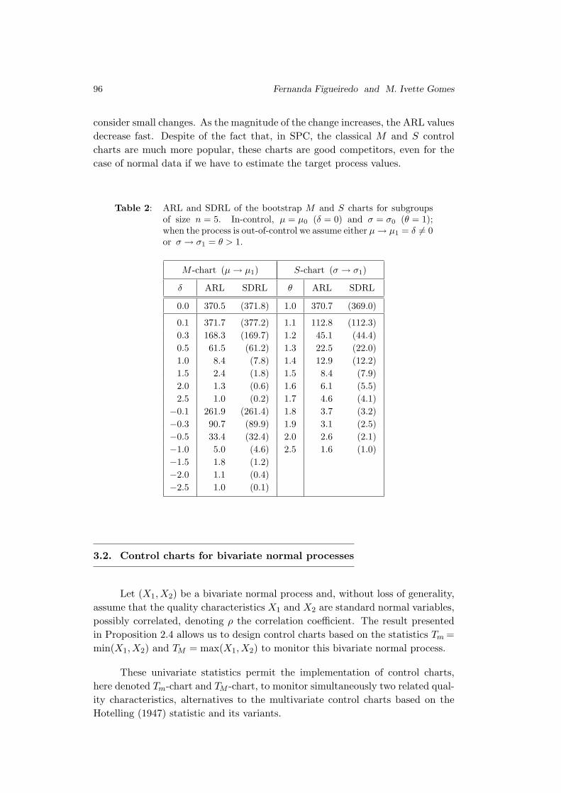
96 Fernanda Figueiredo and M. Ivette Gomes
consider small changes. As the magnitude of the change increases, the ARL values
decrease fast. Despite of the fact that, in SPC, the classical M and S control
charts are much more popular, these charts are good competitors, even for the
case of normal data if we have to estimate the target process values.
Table 2: ARL and SDRL of the bootstrap M and S charts for subgroups
of size n = 5. In-control, µ = µ0 (δ = 0) and σ = σ0 (θ = 1);
when the process is out-of-control we assume either µ → µ1 = δ 6= 0
or σ → σ1 = θ > 1.
M -chart (µ → µ1) S-chart (σ → σ1)
δ ARL SDRL θ ARL SDRL
0.0 370.5 (371.8) 1.0 370.7 (369.0)
0.1 371.7 (377.2) 1.1 112.8 (112.3)
0.3 168.3 (169.7) 1.2 45.1 (44.4)
0.5 61.5 (61.2) 1.3 22.5 (22.0)
1.0 8.4 (7.8) 1.4 12.9 (12.2)
1.5 2.4 (1.8) 1.5 8.4 (7.9)
2.0 1.3 (0.6) 1.6 6.1 (5.5)
2.5 1.0 (0.2) 1.7 4.6 (4.1)
−0.1 261.9 (261.4) 1.8 3.7 (3.2)
−0.3 90.7 (89.9) 1.9 3.1 (2.5)
−0.5 33.4 (32.4) 2.0 2.6 (2.1)
−1.0 5.0 (4.6) 2.5 1.6 (1.0)
−1.5 1.8 (1.2)
−2.0 1.1 (0.4)
−2.5 1.0 (0.1)
3.2. Control charts for bivariate normal processes
Let (X1, X2) be a bivariate normal process and, without loss of generality,
assume that the quality characteristics X1 and X2 are standard normal variables,
possibly correlated, denoting ρ the correlation coefficient. The result presented
in Proposition 2.4 allows us to design control charts based on the statistics Tm =
min(X1, X2) and TM = max(X1, X2) to monitor this bivariate normal process.
These univariate statistics permit the implementation of control charts,
here denoted Tm-chart and TM -chart, to monitor simultaneously two related qual-
ity characteristics, alternatives to the multivariate control charts based on the
Hotelling (1947) statistic and its variants.
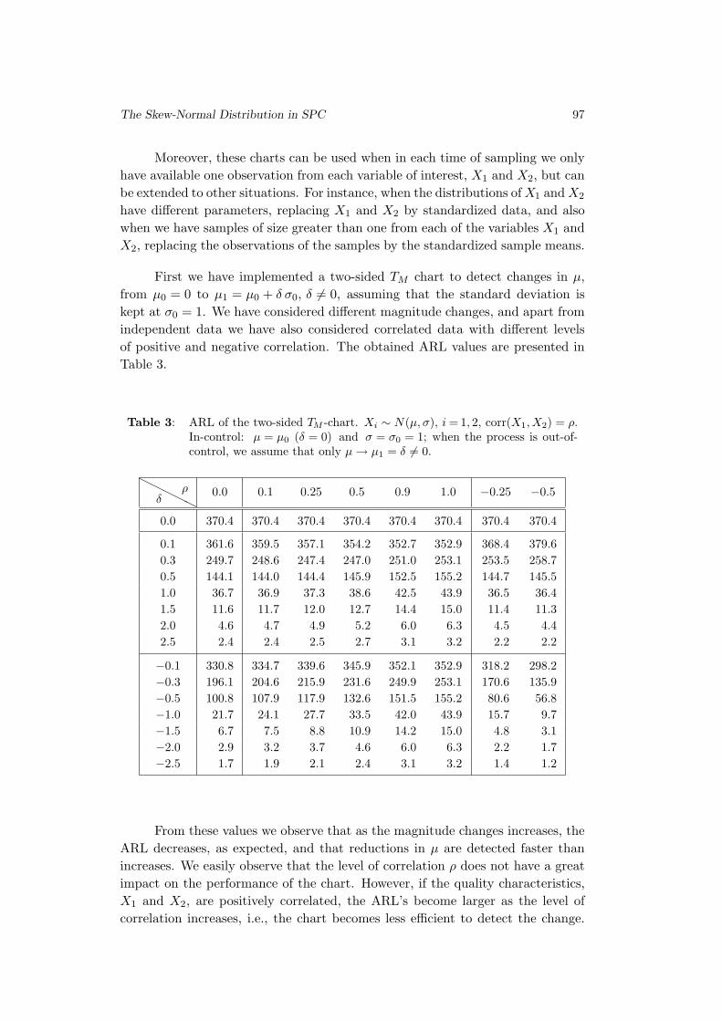
The Skew-Normal Distribution in SPC 97
Moreover, these charts can be used when in each time of sampling we only
have available one observation from each variable of interest, X1 and X2, but can
be extended to other situations. For instance, when the distributions of X1 and X2
have different parameters, replacing X1 and X2 by standardized data, and also
when we have samples of size greater than one from each of the variables X1 and
X2, replacing the observations of the samples by the standardized sample means.
First we have implemented a two-sided TM chart to detect changes in µ,
from µ0 = 0 to µ1 = µ0 + δ σ0, δ 6= 0, assuming that the standard deviation is
kept at σ0 = 1. We have considered different magnitude changes, and apart from
independent data we have also considered correlated data with different levels
of positive and negative correlation. The obtained ARL values are presented in
Table 3.
Table 3: ARL of the two-sided TM -chart. Xi ∼ N(µ, σ), i = 1, 2, corr(X1, X2) = ρ.
In-control: µ = µ0 (δ = 0) and σ = σ0 = 1; when the process is out-of-
control, we assume that only µ → µ1 = δ 6= 0.
HH
HH
Hδ
ρ 0.0 0.1 0.25 0.5 0.9 1.0 −0.25 −0.5
0.0 370.4 370.4 370.4 370.4 370.4 370.4 370.4 370.4
0.1 361.6 359.5 357.1 354.2 352.7 352.9 368.4 379.6
0.3 249.7 248.6 247.4 247.0 251.0 253.1 253.5 258.7
0.5 144.1 144.0 144.4 145.9 152.5 155.2 144.7 145.5
1.0 36.7 36.9 37.3 38.6 42.5 43.9 36.5 36.4
1.5 11.6 11.7 12.0 12.7 14.4 15.0 11.4 11.3
2.0 4.6 4.7 4.9 5.2 6.0 6.3 4.5 4.4
2.5 2.4 2.4 2.5 2.7 3.1 3.2 2.2 2.2
−0.1 330.8 334.7 339.6 345.9 352.1 352.9 318.2 298.2
−0.3 196.1 204.6 215.9 231.6 249.9 253.1 170.6 135.9
−0.5 100.8 107.9 117.9 132.6 151.5 155.2 80.6 56.8
−1.0 21.7 24.1 27.7 33.5 42.0 43.9 15.7 9.7
−1.5 6.7 7.5 8.8 10.9 14.2 15.0 4.8 3.1
−2.0 2.9 3.2 3.7 4.6 6.0 6.3 2.2 1.7
−2.5 1.7 1.9 2.1 2.4 3.1 3.2 1.4 1.2
From these values we observe that as the magnitude changes increases, the
ARL decreases, as expected, and that reductions in µ are detected faster than
increases. We easily observe that the level of correlation ρ does not have a great
impact on the performance of the chart. However, if the quality characteristics,
X1 and X2, are positively correlated, the ARL’s become larger as the level of
correlation increases, i.e., the chart becomes less efficient to detect the change.
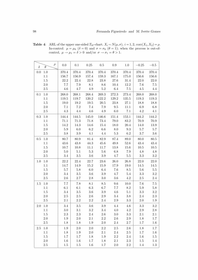
98 Fernanda Figueiredo and M. Ivette Gomes
Table 4: ARL of the upper one-sided TM -chart. Xi ∼N(µ,σ), i = 1, 2, corr(X1,X2) = ρ.
In-control: µ = µ0 (δ = 0) and σ = σ0 (θ = 1); when the process is out-of-
control, µ → µ1 = δ > 0 and/or σ → σ1 = θ > 1.
PP
PP
PP
PPδ θ
ρ 0.0 0.1 0.25 0.5 0.9 1.0 −0.25 −0.5
0.0 1.0 370.4 370.4 370.4 370.4 370.4 370.4 370.4 370.4
1.1 156.7 156.9 157.4 159.3 167.1 175.0 156.6 156.6
1.5 22.2 22.4 22.8 23.8 27.6 31.4 22.0 22.0
2.0 7.7 7.9 8.1 8.6 10.4 12.2 7.6 7.5
2.5 4.6 4.7 4.9 5.2 6.4 7.5 4.5 4.4
0.1 1.0 268.0 268.1 268.4 269.3 272.3 273.4 268.0 268.0
1.1 119.5 119.7 120.2 122.2 129.2 135.5 119.3 119.3
1.5 19.0 19.2 19.5 20.5 23.8 27.1 18.8 18.8
2.0 7.1 7.2 7.4 7.9 9.5 11.1 6.9 6.8
2.5 4.3 4.4 4.6 4.9 6.0 7.1 4.2 4.1
0.3 1.0 144.4 144.5 145.0 146.6 151.4 153.1 144.2 144.2
1.1 71.1 71.3 71.8 73.4 79.0 83.2 70.9 70.9
1.5 14.2 14.3 14.6 15.4 18.0 20.4 14.0 13.9
2.0 5.9 6.0 6.2 6.6 8.0 9.3 5.7 5.7
2.5 3.8 3.9 4.1 4.4 5.3 6.2 3.7 3.6
0.5 1.0 80.7 80.9 81.4 82.9 87.4 89.0 80.0 80.5
1.1 43.6 43.8 44.3 45.6 49.8 52.6 43.4 43.4
1.5 10.7 10.8 11.1 11.7 13.8 15.6 10.5 10.5
2.0 5.0 5.1 5.3 5.6 6.8 7.9 4.8 4.8
2.5 3.4 3.5 3.6 3.9 4.7 5.5 3.3 3.2
1.0 1.0 22.2 22.4 22.7 23.6 26.0 26.8 22.0 22.0
1.1 14.7 14.9 15.2 15.9 17.9 19.0 14.5 14.5
1.5 5.7 5.8 6.0 6.4 7.6 8.5 5.6 5.5
2.0 3.4 3.5 3.6 3.9 4.7 5.4 3.3 3.2
2.5 2.6 2.7 2.8 3.0 3.6 4.2 2.5 2.4
1.5 1.0 7.7 7.8 8.1 8.5 9.6 10.0 7.6 7.5
1.1 6.1 6.1 6.3 6.7 7.7 8.2 5.9 5.8
1.5 3.4 3.5 3.6 3.9 4.6 5.1 3.3 3.2
2.0 2.5 2.5 2.6 2.9 3.4 3.8 2.4 2.3
2.5 2.1 2.2 2.2 2.4 2.9 3.3 2.0 1.9
2.0 1.0 3.4 3.5 3.6 3.9 4.4 4.6 3.3 3.2
1.1 3.0 3.1 3.2 3.4 4.0 4.2 2.9 2.8
1.5 2.3 2.3 2.4 2.6 3.0 3.3 2.1 2.1
2.0 1.9 2.0 2.1 2.2 2.6 2.9 1.8 1.7
2.5 1.8 1.8 1.9 2.0 2.4 2.7 1.7 1.6
2.5 1.0 1.9 2.0 2.0 2.2 2.5 2.6 1.8 1.7
1.1 1.8 1.9 2.0 2.1 2.4 2.5 1.7 1.6
1.5 1.7 1.7 1.8 1.9 2.2 2.4 1.6 1.5
2.0 1.6 1.6 1.7 1.8 2.1 2.3 1.5 1.4
2.5 1.5 1.5 1.6 1.7 2.0 2.2 1.4 1.3
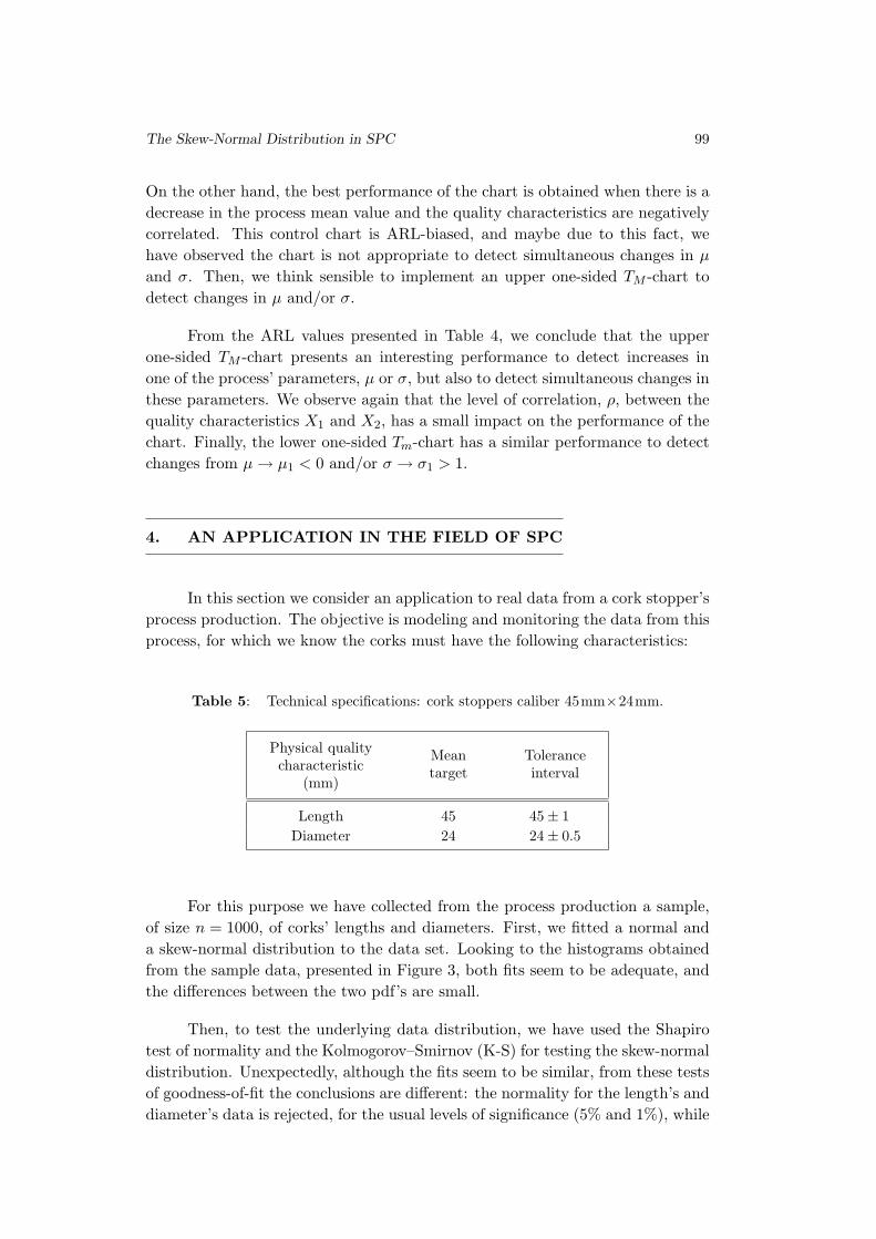
The Skew-Normal Distribution in SPC 99
On the other hand, the best performance of the chart is obtained when there is a
decrease in the process mean value and the quality characteristics are negatively
correlated. This control chart is ARL-biased, and maybe due to this fact, we
have observed the chart is not appropriate to detect simultaneous changes in µ
and σ. Then, we think sensible to implement an upper one-sided TM -chart to
detect changes in µ and/or σ.
From the ARL values presented in Table 4, we conclude that the upper
one-sided TM -chart presents an interesting performance to detect increases in
one of the process’ parameters, µ or σ, but also to detect simultaneous changes in
these parameters. We observe again that the level of correlation, ρ, between the
quality characteristics X1 and X2, has a small impact on the performance of the
chart. Finally, the lower one-sided Tm-chart has a similar performance to detect
changes from µ → µ1 < 0 and/or σ → σ1 > 1.
4. AN APPLICATION IN THE FIELD OF SPC
In this section we consider an application to real data from a cork stopper’s
process production. The objective is modeling and monitoring the data from this
process, for which we know the corks must have the following characteristics:
Table 5: Technical specifications: cork stoppers caliber 45mm×24mm.
Physical quality
characteristic
(mm)
Mean
target
Tolerance
interval
Length 45 45 ± 1
Diameter 24 24 ± 0.5
For this purpose we have collected from the process production a sample,
of size n = 1000, of corks’ lengths and diameters. First, we fitted a normal and
a skew-normal distribution to the data set. Looking to the histograms obtained
from the sample data, presented in Figure 3, both fits seem to be adequate, and
the differences between the two pdf’s are small.
Then, to test the underlying data distribution, we have used the Shapiro
test of normality and the Kolmogorov–Smirnov (K-S) for testing the skew-normal
distribution. Unexpectedly, although the fits seem to be similar, from these tests
of goodness-of-fit the conclusions are different: the normality for the length’s and
diameter’s data is rejected, for the usual levels of significance (5% and 1%), while
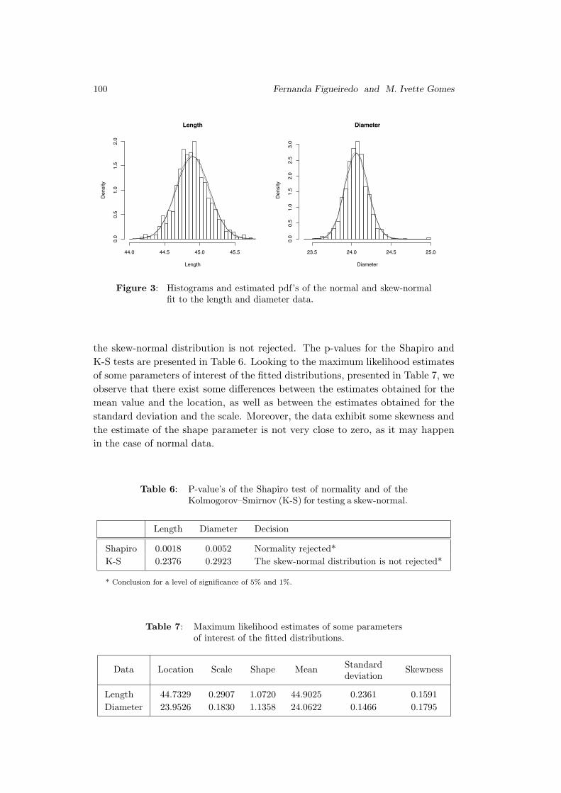
100 Fernanda Figueiredo and M. Ivette Gomes
Length
Length
Density
44.0 44.5 45.0 45.5
0.0
0.5
1.0
1.5
2.0
Diameter
Diameter
Density
23.5 24.0 24.5 25.0
0.0
0.5
1.0
1.5
2.0
2.5
3.0
Figure 3: Histograms and estimated pdf’s of the normal and skew-normal
fit to the length and diameter data.
the skew-normal distribution is not rejected. The p-values for the Shapiro and
K-S tests are presented in Table 6. Looking to the maximum likelihood estimates
of some parameters of interest of the fitted distributions, presented in Table 7, we
observe that there exist some differences between the estimates obtained for the
mean value and the location, as well as between the estimates obtained for the
standard deviation and the scale. Moreover, the data exhibit some skewness and
the estimate of the shape parameter is not very close to zero, as it may happen
in the case of normal data.
Table 6: P-value’s of the Shapiro test of normality and of the
Kolmogorov–Smirnov (K-S) for testing a skew-normal.
Length Diameter Decision
Shapiro 0.0018 0.0052 Normality rejected*
K-S 0.2376 0.2923 The skew-normal distribution is not rejected*
* Conclusion for a level of significance of 5% and 1%.
Table 7: Maximum likelihood estimates of some parameters
of interest of the fitted distributions.
Data Location Scale Shape MeanStandard
deviationSkewness
Length 44.7329 0.2907 1.0720 44.9025 0.2361 0.1591
Diameter 23.9526 0.1830 1.1358 24.0622 0.1466 0.1795
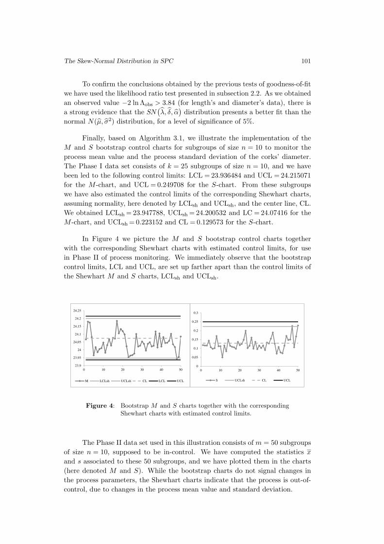
The Skew-Normal Distribution in SPC 101
To confirm the conclusions obtained by the previous tests of goodness-of-fit
we have used the likelihood ratio test presented in subsection 2.2. As we obtained
an observed value −2 ln Λobs > 3.84 (for length’s and diameter’s data), there is
a strong evidence that the SN(λ, δ, α
)distribution presents a better fit than the
normal N(µ, σ2) distribution, for a level of significance of 5%.
Finally, based on Algorithm 3.1, we illustrate the implementation of the
M and S bootstrap control charts for subgroups of size n = 10 to monitor the
process mean value and the process standard deviation of the corks’ diameter.
The Phase I data set consists of k = 25 subgroups of size n = 10, and we have
been led to the following control limits: LCL = 23.936484 and UCL = 24.215071
for the M -chart, and UCL = 0.249708 for the S-chart. From these subgroups
we have also estimated the control limits of the corresponding Shewhart charts,
assuming normality, here denoted by LCLsh and UCLsh, and the center line, CL.
We obtained LCLsh = 23.947788, UCLsh = 24.200532 and LC = 24.07416 for the
M -chart, and UCLsh = 0.223152 and CL = 0.129573 for the S-chart.
In Figure 4 we picture the M and S bootstrap control charts together
with the corresponding Shewhart charts with estimated control limits, for use
in Phase II of process monitoring. We immediately observe that the bootstrap
control limits, LCL and UCL, are set up farther apart than the control limits of
the Shewhart M and S charts, LCLsh and UCLsh.
23,9
23,95
24
24,05
24,1
24,15
24,2
24,25
0 10 20 30 40 50
M LCLsh UCLsh CL LCL UCL
0
0,05
0,1
0,15
0,2
0,25
0,3
0 10 20 30 40 50
S UCLsh CL UCL
Figure 4: Bootstrap M and S charts together with the corresponding
Shewhart charts with estimated control limits.
The Phase II data set used in this illustration consists of m = 50 subgroups
of size n = 10, supposed to be in-control. We have computed the statistics x
and s associated to these 50 subgroups, and we have plotted them in the charts
(here denoted M and S). While the bootstrap charts do not signal changes in
the process parameters, the Shewhart charts indicate that the process is out-of-
control, due to changes in the process mean value and standard deviation.

102 Fernanda Figueiredo and M. Ivette Gomes
5. SUMMARY AND RECOMMENDATIONS
Designing a control chart under the assumption of skew-normal data and
with control limits estimated via bootstrapping adds a relevant contribution to
the SPC literature in what concerns the implementation of robust control charts.
The use of this family of distributions, that includes the Gaussian as a particular
member, allows more flexibility to accommodate uncontrollable disturbances in
the data, such as some level of asymmetry or non-normal tail behavior. Moreover,
despite of the fact that, in SPC, the classical M and S control charts are much
more popular, these charts are good competitors, even for the case of normal data
if we have to estimate the target process values.
In order to integrate it within a quality process control system, we can
suggest, for instance, an a priori analysis of the process data. A simple boxplot
representation with the Phase I data subgroups can anticipate an underlying data
distribution that exhibits some level of asymmetry, possibly with some outliers,
and in this case, we suggest the use of the proposed bootstrap control charts
instead of the traditional Shewhart-type charts implemented for normal data.
Among other issues not addressed in this paper, the proposed control charts
should be compared to the existing parametric and nonparametric control charts.
Also important is to study the effect of increasing the Phase I sample on the
performance of the chart, as well as the determination of the minimum number m
of subgroups in Phase I, the sample size n and the number of replicates bootstrap r
we must consider in order to have charts with the same performance for the
scenarios of known and unknown process parameters. Finally, an exhaustive and
comparative study about the performance of control charts based on the skew-
normal and on the normal distributions must be carried out to have an idea about
the range of values of the shape parameter α of the skew-normal distribution for
which the performance of the two charts differ significantly. This will help a
practitioner to make a decision on which control chart is preferable to suit his
needs.
ACKNOWLEDGMENTS
This research was partially supported by national funds through the Fun-
dacao Nacional para a Ciencia e Tecnologia, Portugal — FCT, under the PEst-
OE/MAT/UI0006/2011 project.
We would like to thank to the two anonymous referees the very helpful
comments and suggestions for future research.
The Skew-Normal Distribution in SPC 103
REFERENCES
[1] Abtahi, A.; Towhidi, M. and Behboodian, J. (2011). An appropriate em-
pirical version of skew-normal density, Statistical Papers, 52, 469–489.
[2] Azzalini, A. (1985). A Class of distributions which includes the normal Ones,
Scandinavian J. of Statistics, 12, 171–178.
[3] Azzalini, A. (1986). Further results on a class of distributions which includes
the normal ones, Statistica, XLVI, 199–208.
[4] Azzalini, A. (2005). The skew-normal distribution and related multivariate fam-
ilies, Scandinavian J. of Statistics, 32, 159–188.
[5] Azzalini, A. (2011). R package ‘sn’: The skew-normal and skew-t distributions
(version 0.4-17). URL http://azzalini.stat.unipd.it/SN.
[6] Azzalini, A. and Capitanio, A. (1999). Statistical applications of the multi-
variate skew normal distributions, J. R. Stat. Soc., series B, 61, 579–602.
[7] Azzalini, A. and Regoli, G. (2012). Some properties of skew-symmetric dis-
tributions, Annals of the Institute of Statistical Mathematics, 64, 857–879.
[8] Bai, D.S. and Choi, I.S. (1995). X and R control charts for skewed populations,
J. of Quality Technology, 27(2), 120–131.
[9] Chakraborti, S.; Human, S.W. and Graham, M.A. (2011). Nonparametric
(distribution-free) quality control charts. In “Methods and Applications of Statis-
tics: Engineering, Quality Control, and Physical Sciences”(N. Balakrishnan, Ed.),
298–329.
[10] Chakraborti, S.; Human, S.W. and Graham, M.A. (2009). Phase I statis-
tical process control charts: an overview and some results, Quality Engineering,
21(1), 52–62.
[11] Efron, B. and Tibshirani, R. (1993). Introduction to the Bootstrap, Chapman
and Hall, New York.
[12] Fernandez, C. and Steel, M.F.J. (1998). On Bayesian modeling of fat tails
and skewness, J. Am. Stat. Assoc., 93, 359–371.
[13] Hoaglin, D.M.; Mosteller, F. and Tukey, J.W. (1983). Understanding
Robust and Exploratory Data Analysis, Wiley, New York.
[14] Hotelling, H. (1947). Multivariate quality control illustrated by air testing of
sample bombsights. In “Selected Techniques of Statistical Analysis” (C. Eisenhart,
M.W. Hastay and W.A. Wallis, Eds.), pp. 111–184, McGraw-Hill, New York.
[15] Human, S.W. and Chakraborti, S. (2010). A unified approach for Shewhart-
type phase I control charts for the mean, International Journal of Reliability,
Quality and Safety Engineering, 17(3), 199–208.
[16] Jamalizadeb, A.; Arabpour, A.R. and Balakrishnan, N. (2011). A gener-
alized skew two-piece skew normal distribution, Statistical Papers, 52, 431–446.
[17] Jones, L.A. and Woodall, W.H. (1998). The performance of bootstrap con-
trol charts, J. of Quality Technology, 30, 362–375.
[18] Lio, Y.L. and Park, C. (2008). A bootstrap control chart for Birnbaum–
Saunders percentiles, Qual. Reliab. Engng. Int., 24, 585–600.
104 Fernanda Figueiredo and M. Ivette Gomes
[19] Lio, Y.L. and Park, C. (2010). A bootstrap control chart for inverse Gaussian
percentiles, J. of Statistical Computation and Simulation, 80(3), 287–299.
[20] Liu, R.Y. and Tang, J. (1996). Control charts for dependent and independent
measurements based on the bootstrap, JASA, 91, 1694–1700.
[21] Montgomery, D.C. (2005). Introduction to Statistical Quality Control, Wiley,
New York.
[22] Nichols, M.D. and Padgett, W.J. (2006). A bootstrap control chart for
Weibull percentiles, Qual. Reliab. Engng. Int., 22, 141–151.
[23] O’Hagan, A. and Leonard, T. (1976). Bayes estimation subject to uncertainty
about parameter constraints, Biometrika, 63, 201–202.
[24] Owen, D.B. (1956). Tables for computing bivariate normal probabilities, Ann.
Math. Statist., 27, 1075–1090.
[25] Seppala, T.; Moskowitz, H.; Plante, R. and Tang, J. (1995). Statistical
process control via the subgroup bootstrap, J. of Quality Technology, 27, 139–153.
REVSTAT – Statistical Journal
Volume 11, Number 1, March 2013, 105–119
IMPROVING SSA PREDICTIONS BY INVERSE
DISTANCE WEIGHTING
Authors: Richard O. Awichi
– Uganda Martyrs University, Nkozi, Uganda
Werner G. Muller
– Johannes Kepler University, Linz, Austria
Abstract:
• This paper proposes a method of utilizing spatial information to improve predictions
in one dimensional time series analysis using singular spectrum analysis (SSA). It em-
ploys inverse distance weighting for spatial averaging and subsequently multivariate
singular spectrum analysis (MSSA) for enhanced forecasts. The technique is exempli-
fied on a data set for rainfall recordings from Upper Austria.
Key-Words:
• singular spectrum analysis; inverse distance weighting; spatio-temporal predictions.
AMS Subject Classification:
• 49A05, 78B26.

106 R. Awichi and W.G. Muller
Inverse Distance Weighting SSA 107
1. INTRODUCTION
Singular spectrum analysis (SSA) is a recently popularized tool for time
series analysis, cf. [10]. The origins of SSA can be traced to [2, 4, 6]. More infor-
mation about the history of SSA can be found in [22]. It is a model free approach
to time series analysis and literally any time series with a notable structure can be
analysed using SSA. Indeed it has a wide area of applications ranging from mathe-
matics and physics [10], to economics and financial mathematics [13, 14], environ-
mental sciences [15], social sciences [12], and medicine [7]. It is now implemented
under various software platforms, here we use Rssa, see [9] and a program called
CaterpilarSSA as can be downloaded from http://www.gistatgroup.com/cat/
programs.html. The aim of SSA is twofold:
i) To make a decomposition of the original series into a sum of a small
number of independent and interpretable components such as a slowly
varying trend, oscillatory components and a structure less noise;
ii) To reconstruct the decomposed series so as to make predictions without
the noise component.
MSSA is an extension of SSA and takes advantage of the (delay) embedding
procedure to obtain a similar formulation as SSA, albeit with larger matrices for
multidimensional time series. It has previously been successfully applied to the
study of climate fields, see [18]. Here we will employ it to jointly model an original
time series with a spatial average of which we believe will improve predictions by
pooling spatially dependent information.
One of the simplest but effective ways of generating spatial averages is
inverse distance weighting, which was first introduced, incidentally also for the
analysis of rainfall data in [11]. It was subsequently propagated in [20] and
became thereafter one of the most popular spatial interpolation techniques
(cf. eg. [16]).
Section 2 is devoted to reviewing the basics of SSA. Section 3 discusses
forecasting, while Section 4 briefly presents MSSA, an extension of the SSA tech-
niques to multivariate data and introduces a method of incorporating spatial
dependence to improve forecasts. The application is presented in Section 5 and
conclusions appear in Section 6.
2. SINGULAR SPECTRUM ANALYSIS
Most classical time series models devised for analysis and forecasting are
based on restrictive assumptions of normality, linearity and stationarity, cf. [3].
108 R. Awichi and W.G. Muller
A number of time series are deterministic, linear and dynamical systems thus
allowing linear models to be used for modelling and forecasting. However, many
time series exhibit nonlinear behaviour and therefore would require a method
that works well for both linear and nonlinear, stationary and nonstationary data
sets. SSA is one such technique.
2.1. A brief review of SSA
The Basic SSA, as it is commonly referred to, has two main stages: De-
composition and Reconstruction; each of which consists of two steps as described
below. The main concept in SSA is the aspect of separability of the original time
series into signal and noise so that the analysis and forecasting can be done on
signal in the absence of noise. Separability will be mentioned again later. In the
following discussion, we follow the approach in [10, Chapter 1].
Let FN = {f1, f2, ..., fN} be a real valued, nonzero (at least one fi 6= 0)
time series data of sufficient length N without missing values.
Stage 1: Decomposition
Step 1: Embedding
This (standard) time series procedure maps the one dimensional time series,
FN into multidimensional lagged vectors, X1 : ··· : XK , where
Xi = (f1, ..., fi+L−1)T ∈ RL , 1 ≤ i ≤ K and K = N − L + 1 .
The single most important parameter of embedding is the window length, L, an
integer such that 2 < L < N . This parameter should always be large enough to
permit reasonable separability. It should not be greater the N/2 for optimum
results. See [8] for more on the choice of parameters for SSA. The vectors Xi,
called the lagged vectors or L lagged vectors (to emphasize their dimension) form
the K columns of the trajectory matrix X, i.e. X = [X1 : ··· : XK ].
Specifically X is given as follows:
X =
f1 f2 f3 ··· fK
f2 f3 f4 ··· fK+1
f3 f4 f5 ··· fK+2...
. . ....
. . ....
fL fL+1 fL+2 ··· fN
.
The L×K matrix X is a Hankel matrix, i.e. the elements along the anti-diagonal,
i + j = constant are equal, for the ith row and j thcolumn.
Inverse Distance Weighting SSA 109
Step 2: Singular Value Decomposition, SVD
This decomposes the trajectory matrix X and represents it as a sum of
elementary matrices (rank-one bi-orthogonal). This is done by:
i) Calculating the matrix S = XXT.
ii) Obtaining eigenvalues, λi of S such that λ1 ≥ λ2 ≥ ··· ≥ λL ≥ 0. Since
S is positive definite, the eigenvalues are positive.
iii) For each λi, calculate Ui and Vi, the left and right singular vectors
of X. The Ui s are orthonormal system of eigenvectors corresponding
to each λi such that 〈Ui, Uj〉 = 0, i 6= j (orthogonality) and ‖Ui‖ = 1
(unit norm property) and Vi = XT Ui/√
λi.
iv) Set d = max(i : λi > 0) = rank(X). Then Xi =√
λi UiVTi (i = 1, ..., d),
and the SVD of the trajectory matrix represents it as a sum of the Xi,
i.e.:
X =
d∑
i=1
Xi
= X1 + X2 + ··· + Xd .
(2.1)
The collection (√
λi, Ui, Vi) is called the ith eigentriple of X,√
λi are the singular
values of X and the set{√
λi
}d
i=1is the spectrum of X.
The ratio λi
/ d∑i=1
λi is the characteristic contribution (or its share) of Xi to (2.1).
The first eigenvalue has the largest contribution and the last has the smallest.
If all the eigenvalues have multiplicity one, then (2.1) is uniquely determined.
Stage 2: Reconstruction
Step 3: Grouping
This corresponds to splitting the elementary matrices Xi into several groups
and summing the matrices within each group. If I = i1, ..., ip be one such group,
then the matrix XI corresponding to the group I is defined as:
XI = Xi1 + ··· + Xip .
For m such groups (disjoint), then X will be given as:
(2.2) X = XI1 + ··· + XIm.
Matrices XIiare called resultant matrices and the procedure of choosing the sets
I1, ..., Im is called the eigentriple grouping.
The contribution of component XI in (2.2) is measured by the share of the cor-
responding eigenvalues, i.e.∑i∈I
λi
/ d∑i=1
λi.
110 R. Awichi and W.G. Muller
Step 4: Diagonal Averaging
This (last) step transfers each resultant matrix into a time series, which
is an additive component of the initial (original) series, FN . If zij stands for an
element of a matrix Z, then the kthterm of the resulting series is obtained by
averaging zij over all i, j such that i+ j = k +2 ([10, page 17, 24], [12, page 242]).
This is diagonal averaging or Hankelization of the matrix Z. The result of the
Hankelization of a matrix Z is the matrix HZ. Diagonal averaging is a linear
operation and maps the trajectory matrix of the initial series into the original
series itself, i.e. it transfers each matrix I into a time series which is an additive
component of the initial series FN .
2.2. Separability
As mentioned earlier, the main concept in studying SSA properties is sepa-
rability. This entails how well the components of the time series can be separated
from each other to allow forecasting to be meaningfully done and also reliable
construction of confidence bounds. Any time series may comprise trend (slowly
varying component), periodic or quasi periodic components (like seasonal varia-
tions or harmonics generally) and noise. These may be generalized into signal and
noise components. SSA decomposition of the series FN can only be successful if
the resulting additive components of the series are approximately separable from
each other, [10, 12].
If a time series FN can be split as FN = F(1)N + F
(2)N , then the matrix terms
of the SVD step can be split into X(1)and X(2)
respectively, i.e. X = X(1)+X(2)
.
This would imply that each row of X(1)is orthogonal to each row of X(2)
. Since
rows (and columns) of the trajectory matrix X are themselves subseries of the
initial series, the orthogonality condition of the rows of X(1)and X(2)
is the condi-
tion of orthogonality of any subseries of length L and K = N −L + 1 of the series
F(1)N to any subseries of the same length, F
(2)N . If this holds, then F
(1)N and F
(2)N
are said to be weakly separable.
In geometrical terms, F(1)N and F
(2)N are separable if and only if the subspace
ℓ(L,1)spanned by the columns of X(1)
is orthogonal to the subspace ℓ(L,2)spanned
by the columns of X(2). One way to enhance separability of the series is auxiliary
information about the series to help in choosing the window length, for example,
if it is known that there is a seasonal component whose period is an integer,
it is advisable to choose the window length which is a factor of the period, [10,
page 44]. To choose eigentriples, one may use the graph of the logarithms of
eigenvalues in which explicit plateau in the eigenvalue spectra prompts ordinal
numbers of the eigentriple and a slowly decreasing sequence of singular values
corresponds to noise components.
Inverse Distance Weighting SSA 111
Another way to measure the separability between two series components,
F(1)N and F
(2)N (i.e. if FN = F
(1)N + F
(2)N ) is to calculate the weighted correlation or
w-correlations between the two using the formula
ρw12 =
⟨F
(1)N , F
(2)N
⟩w∥∥F
(1)N
∥∥w
∥∥F(2)N
∥∥w
,
where∥∥F
(i)N
∥∥w
=
√⟨F
(i)N , F
(i)N
⟩w, i = 1, 2,
⟨F
(1)N , F
(2)N
⟩w
=
N−1∑i=0
wif(1)i f
(2)i , and
the weights wi defined as follows:
Let L⋆= min(L, K) and K⋆
= max(L, K). Then,
wi =
i + 1 for 0 6 i 6 L⋆ − 1 ,
L⋆for L⋆ 6 i 6 K⋆ ,
N − i for K⋆ 6 i 6 N − 1 .
A natural hint for grouping is the matrix of the absolute values of the w-corre-
lations corresponding to a full decomposition. If the absolute value of the
w-correlation is small then the corresponding series are almost w-orthogonal
and is said to be weakly separable. The series F (1)and F (2)
are w-orthogonal if⟨F
(1)N , F
(2)N
⟩w
= 0, [10, 12].
Separability is analogous to independence of random variables whence the
covariance and correlation between such random variables are zero, [5, Section 4.5].
3. FORECASTING WITH SSA
Details of SSA Forecasting can be found in [10, Chapter 2, 5] and in [19].
We have three basic conditions:
1) Time series has structure.
2) A mechanism identifying this structure is found.
3) A method of time series continuation, based on the identified structure
is available.
In SSA, forecasting is done through application of linear recurrent formulae
(LRF) or equations. The class of series governed by LRF is rather wide; it
contains harmonics, polynomials and exponential series and is closed under term-
by-term addition and multiplication, [12]. An infinite series is governed by some
LRF if and only if it can be represented as a linear combination of products
112 R. Awichi and W.G. Muller
of exponential, polynomial and harmonic series. (The signal component of a
separable time series is always a linear combination of these series.)
An important property of SSA decomposition is that the original series
satisfies an LRF of the form fn = a1fn−1 + ··· + adfn−d for some dimension d;
a1, ..., ad are constants.
Thus for any N and L, there are at most d nonzero singular values in the
SVD of the trajectory matrix X and so even if L and K = N − L + 1 are larger
than d, we need at most d matrices Xi to reconstruct the series. If fn satisfies the
LRF above, it will always be represented as a sum of products of exponentials,
polynomials and harmonics, [10].
Alternatively put, if r < L, (r = number of terms in the SVD step), then
the series satisfies some LRF of some dimension d 6 r. This result also implies
that if dim(ℓr) < L, then the series satisfies a natural LRF of dimension L − 1.
Any such series satisfying an LRF can then be forecast for an arbitrary number
of steps using the LRF.
The selection of the resultant matrices in the third step of Basic SSA algo-
rithm implies selection of the r-dimensional space ℓr ∈ RLspanned by the corre-
sponding left singular vectors and if ℓr is non-vertical, it produces an appropriate
LRF which can be used in forecasting.
An LRF that governs a series with the help of SSA may be found as follows.
Let d be minimal dimension of all LRFs governing a time series FN . If the window
length L is greater than d and N is large enough, then the trajectory space of FN
is d dimensional. The trajectory space determines an LRF of dimension L − 1
that governs the time series. If this LRF is applied to the last terms of the
series, a forecast of the series is obtained. The same idea works for an additive
component F(1)N of FN . The assumption here is that F
(1)N is (strongly) separable
from the residual F(2)N = FN − F
(1)N for the selected window length L. Normally
(strong) separability of the components of a series implies that each component
satisfies some LRF, [10, Chapter 6]. If F(2)N is noise, then forecasting is done
for F(1)N . Thus using a selected set of eigentriples, estimation can be performed
on F(1)N and its trajectory space. The basic inputs for the SSA LRF for a series
FN include the window length L, N , linear space ℓv which is not a vertical space
and the number M of points to forecast. The linear space is used to obtain an
orthonormal basis P1, ..., Pr used in the forecasting process.
Forecasting is also closely linked to separability of the series as mentioned
above. If FN = F(1)N + F
(2)N , then forecasting is done for the signal F
(1)N in the
presence of the noise component F(2)N which is given as F
(2)N = FN − F
(1)N .
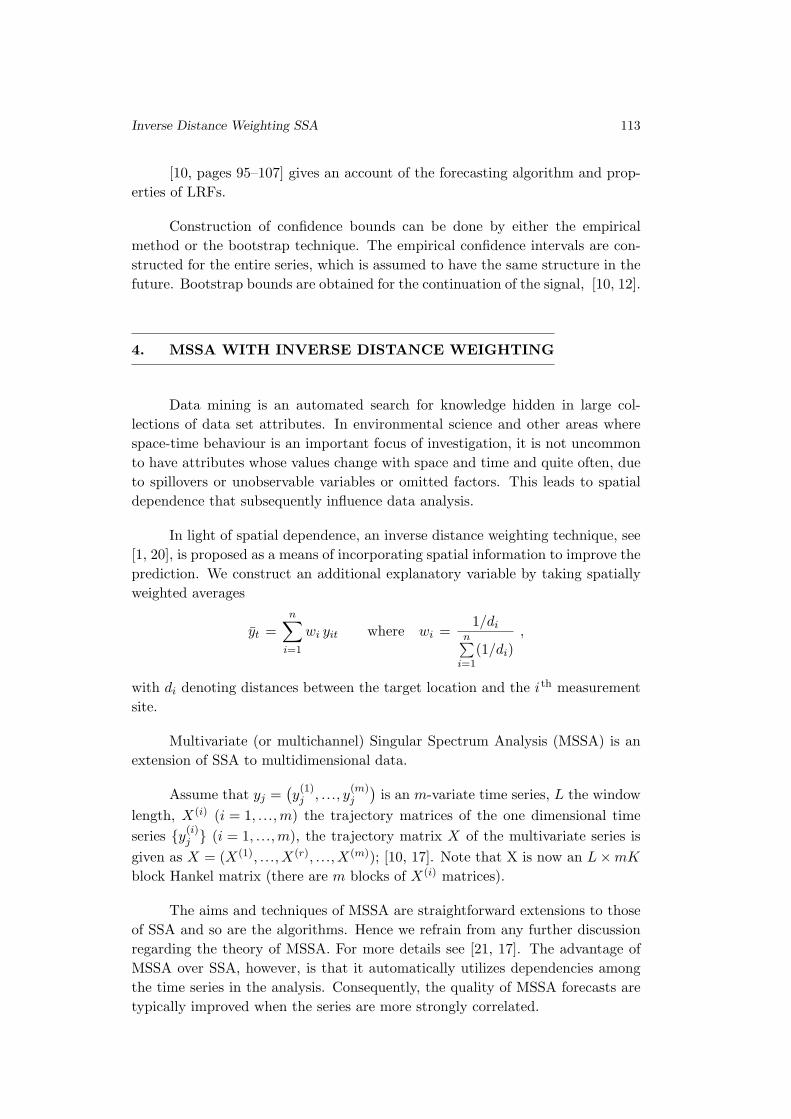
Inverse Distance Weighting SSA 113
[10, pages 95–107] gives an account of the forecasting algorithm and prop-
erties of LRFs.
Construction of confidence bounds can be done by either the empirical
method or the bootstrap technique. The empirical confidence intervals are con-
structed for the entire series, which is assumed to have the same structure in the
future. Bootstrap bounds are obtained for the continuation of the signal, [10, 12].
4. MSSA WITH INVERSE DISTANCE WEIGHTING
Data mining is an automated search for knowledge hidden in large col-
lections of data set attributes. In environmental science and other areas where
space-time behaviour is an important focus of investigation, it is not uncommon
to have attributes whose values change with space and time and quite often, due
to spillovers or unobservable variables or omitted factors. This leads to spatial
dependence that subsequently influence data analysis.
In light of spatial dependence, an inverse distance weighting technique, see
[1, 20], is proposed as a means of incorporating spatial information to improve the
prediction. We construct an additional explanatory variable by taking spatially
weighted averages
yt =
n∑
i=1
wi yit where wi =1/di
n∑i=1
(1/di)
,
with di denoting distances between the target location and the i thmeasurement
site.
Multivariate (or multichannel) Singular Spectrum Analysis (MSSA) is an
extension of SSA to multidimensional data.
Assume that yj =(y
(1)j , ..., y
(m)j
)is an m-variate time series, L the window
length, X(i)(i = 1, ..., m) the trajectory matrices of the one dimensional time
series {y(i)j } (i = 1, ..., m), the trajectory matrix X of the multivariate series is
given as X = (X(1), ..., X(r), ..., X(m)); [10, 17]. Note that X is now an L × mK
block Hankel matrix (there are m blocks of X(i)matrices).
The aims and techniques of MSSA are straightforward extensions to those
of SSA and so are the algorithms. Hence we refrain from any further discussion
regarding the theory of MSSA. For more details see [21, 17]. The advantage of
MSSA over SSA, however, is that it automatically utilizes dependencies among
the time series in the analysis. Consequently, the quality of MSSA forecasts are
typically improved when the series are more strongly correlated.

114 R. Awichi and W.G. Muller
The above pooling of the spatial information by inverse distance weighting
leads to a new time series yt that can be used as a kind of covariable to the Linz
rainfall series to improve the predictions. We thus now employ a MSSA with the
original Linz series complemented by the pooled one, i.e. m = 2 in this case. Of
course this can be performed for all the time series, not only the Linz one and
even jointly, but we will refrain from this for the sake of expository simplicity.
5. THE APPLICATION
The complete data set consisted of N = 192 monthly recordings of rainfall
at several locations in Upper Austria for the period 1994 Jan to 2009 Dec (see
Figure 1 for a depiction of the measurement locations with the solid dot indicating
Linz). The data is provided by the Zentralanstalt fur Meteorologie in Austria and
is described in more detail in [15].
Figure 1: Upper-Austrian rainfall measurement network.
Empty circle indicate measurement locations, solid circle Linz.
The time series graph Figure 2 shows the general behaviour of the logarithm
of Linz rainfall series and the reconstructed series for the period above. Since it is
annual data, it provides auxiliary information for the choice of the window length
as a factor of the period, 12 monthlies, hence the choice of L = 96 = N/2 as the
standard window length for the analysis. It can be inferred from the figure that
the grouping employed yielded a reconstructed series fairly close to the original
hence rather reliable in-sample predictions.
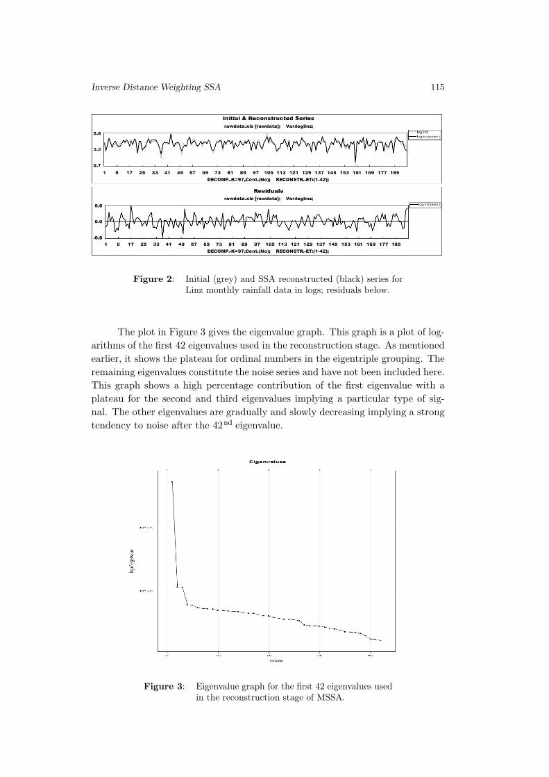
Inverse Distance Weighting SSA 115
Figure 2: Initial (grey) and SSA reconstructed (black) series for
Linz monthly rainfall data in logs; residuals below.
The plot in Figure 3 gives the eigenvalue graph. This graph is a plot of log-
arithms of the first 42 eigenvalues used in the reconstruction stage. As mentioned
earlier, it shows the plateau for ordinal numbers in the eigentriple grouping. The
remaining eigenvalues constitute the noise series and have not been included here.
This graph shows a high percentage contribution of the first eigenvalue with a
plateau for the second and third eigenvalues implying a particular type of sig-
nal. The other eigenvalues are gradually and slowly decreasing implying a strong
tendency to noise after the 42nd
eigenvalue.
Figure 3: Eigenvalue graph for the first 42 eigenvalues used
in the reconstruction stage of MSSA.
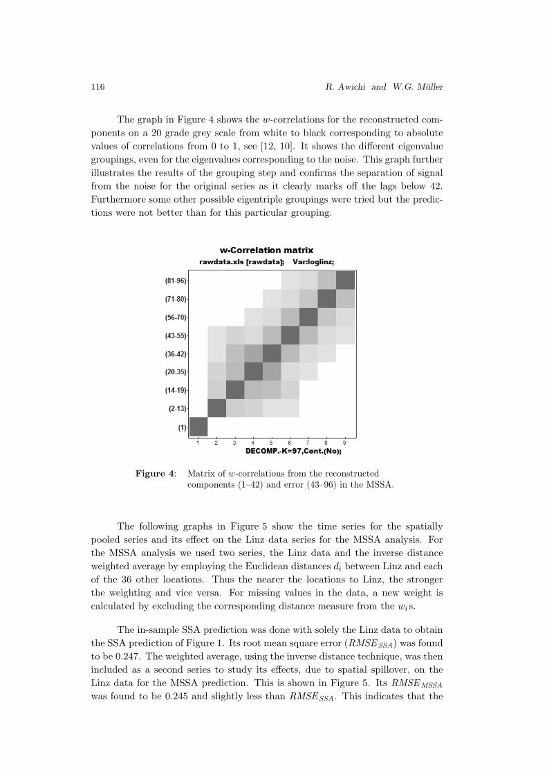
116 R. Awichi and W.G. Muller
The graph in Figure 4 shows the w-correlations for the reconstructed com-
ponents on a 20 grade grey scale from white to black corresponding to absolute
values of correlations from 0 to 1, see [12, 10]. It shows the different eigenvalue
groupings, even for the eigenvalues corresponding to the noise. This graph further
illustrates the results of the grouping step and confirms the separation of signal
from the noise for the original series as it clearly marks off the lags below 42.
Furthermore some other possible eigentriple groupings were tried but the predic-
tions were not better than for this particular grouping.
Figure 4: Matrix of w-correlations from the reconstructed
components (1–42) and error (43–96) in the MSSA.
The following graphs in Figure 5 show the time series for the spatially
pooled series and its effect on the Linz data series for the MSSA analysis. For
the MSSA analysis we used two series, the Linz data and the inverse distance
weighted average by employing the Euclidean distances di between Linz and each
of the 36 other locations. Thus the nearer the locations to Linz, the stronger
the weighting and vice versa. For missing values in the data, a new weight is
calculated by excluding the corresponding distance measure from the wi s.
The in-sample SSA prediction was done with solely the Linz data to obtain
the SSA prediction of Figure 1. Its root mean square error (RMSESSA) was found
to be 0.247. The weighted average, using the inverse distance technique, was then
included as a second series to study its effects, due to spatial spillover, on the
Linz data for the MSSA prediction. This is shown in Figure 5. Its RMSEMSSA
was found to be 0.245 and slightly less than RMSESSA. This indicates that the
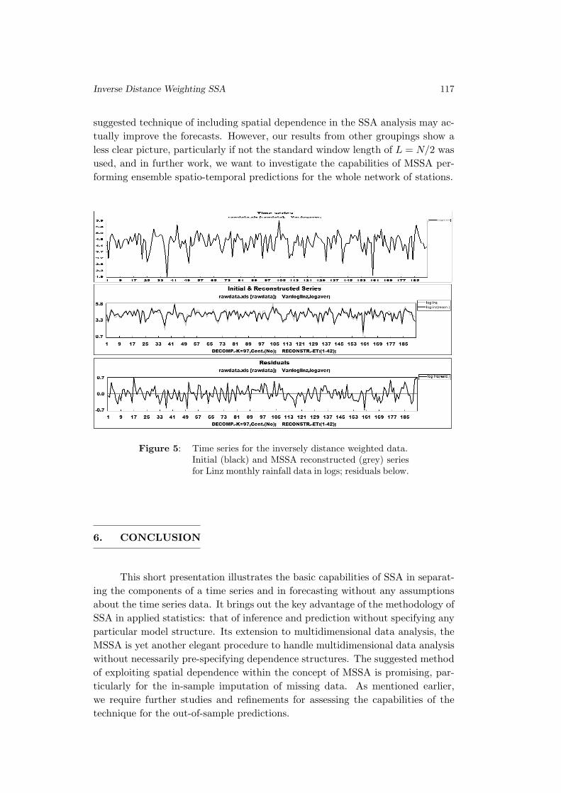
Inverse Distance Weighting SSA 117
suggested technique of including spatial dependence in the SSA analysis may ac-
tually improve the forecasts. However, our results from other groupings show a
less clear picture, particularly if not the standard window length of L = N/2 was
used, and in further work, we want to investigate the capabilities of MSSA per-
forming ensemble spatio-temporal predictions for the whole network of stations.
Figure 5: Time series for the inversely distance weighted data.
Initial (black) and MSSA reconstructed (grey) series
for Linz monthly rainfall data in logs; residuals below.
6. CONCLUSION
This short presentation illustrates the basic capabilities of SSA in separat-
ing the components of a time series and in forecasting without any assumptions
about the time series data. It brings out the key advantage of the methodology of
SSA in applied statistics: that of inference and prediction without specifying any
particular model structure. Its extension to multidimensional data analysis, the
MSSA is yet another elegant procedure to handle multidimensional data analysis
without necessarily pre-specifying dependence structures. The suggested method
of exploiting spatial dependence within the concept of MSSA is promising, par-
ticularly for the in-sample imputation of missing data. As mentioned earlier,
we require further studies and refinements for assessing the capabilities of the
technique for the out-of-sample predictions.
118 R. Awichi and W.G. Muller
ACKNOWLEDGMENTS
We are grateful to the two anonymous referees for their attentive and de-
tailed remarks which helped to considerably improve the paper.
REFERENCES
[1] Bakkali, S. and Amrani, M. (2008). About the use of spatial interpolation
methods to denoising Moroccan resistivity data phosphate ”disturbances” map,
Acta Montanistica Slovaca, 13, 216–222.
[2] Basilevsky, A. and Hum, D.P.J. (1979). Karhunen–Loeve analysis of histor-
ical time series with an application to plantation births in Jamaica, Journal of
American Statistical Association, 74, 284–290.
[3] Brockwell, P.J. and Davis, R.A. (2002). Introduction to Time Series and
Forecasting, Springer, New York.
[4] Broomhead, D.S. and King, G.P. (1986). Extracting qualitative dynamics
from experimental data, Physica D, 20, 217–236.
[5] Casella, G. and Berger, R.L. (2002). Statistical Inference, Second Edition,
Duxbury / Thomson Learning, Australia, USA, Canada.
[6] Elsner, J.B. and Tsonis,A.A. (1996). Singular Spectrum Analysis: A New Tool
in Time Series Analysis, Plenum.
[7] Ghodsi, M.; Hassani, H. and Sanei, S. (2010). Extracting fetal heart signal
from noisy maternal ECG by multivariate singular spectrum analysis, Statistics
and Its Interface, 3, 399–411.
[8] Golyandina, N. (2010). On the choice of parameters in singular spectrum anal-
ysis and related subspace-based methods, Statistics and Its Interface 3, 259–279.
[9] Golyandina, N. and Korobeynikov, A. (2012). Basic singular spectrum anal-
ysis and forecasting with R, arXiv:1206.6910.
[10] Golyandina, N.; Nekrutkin, V. and Zhigljavsky, A. (2001). Analysis of
Time Series Structure: SSA and Related Techniques, Chapman & Hall; CRC,
New York, London.
[11] Horton, R.E. (1923). Rainfall interpolation, Monthly Weather Review, 51(6),
291–304.
[12] Hassani, H. (2007). Singular spectrum analysis: methodology and comparison,
Journal of Data Science, 5, 239–257.
[13] Hassani, H. and Thomakos, D. (2010). A Review on singular spectrum analy-
sis for economic and financial time series, Statistics and Its Interface, 3, 377–397.
[14] Kapl, M. and Muller, W.G. (2010). Prediction of steel prices: a comparison
between a conventional regression model and MSSA, Statistics and Its Interface,
3, 369–275.
Inverse Distance Weighting SSA 119
[15] Mateu, J. and Muller, W.G. (Eds.) (2012). Spatio-temporal Design: Ad-
vances in Efficient Data Acquisition; (Statistics in Practice), Wiley.
[16] Okabe, A. and Sugihara, K. (2012). Spatial Analysis Along Networks: Statis-
tical and Computational Methods; (Statistics in Practice), Wiley.
[17] Patterson, K.; Hassani, H.; Heravi, S. and Zhigljavsky, A. (2011).
Multivariate singular spectrum analysis for forecasting revisions to real-time data,
Journal of Applied Statistics, 38(10), 2183–2211.
[18] Raynaud, S.; Yiou, P.; Kleeman, R. and Speich, S. (2005). Using MSSA to
determine explicitly the oscillatory dynamics of weakly nonlinear climate systems,
Journal of Nonlinear Processes in Geophysics, 12, 807–815.
[19] Rodrigues, P.C. and de Carvalho, M. (2012). Spectral modeling of time
series with missing data, Applied Mathematical Modelling,
http://dx.doi.org/10.1016/j.apm.2012.09.040
[20] Shepard, D. (1968). A two-dimensional interpolation function for irregularly-
spaced data, Proceedings of the 1968 23 rd ACM national conference, ACM ’68,
ACM, New York, NY, USA, pp. 517–524.
[21] Hassani, H.; Heravi, S. and Zhigljavsky, A. (2009). Forecasting european
industrial production with multivariate singular spectrum analysis, International
Journal of Forecasting, 25(1), 103–118.
[22] Zhigljavsky, A. (2010). Singular spectrum analysis for time series, Statistics
and Its Interface, 3, 255–258.


REVSTAT – STATISTICAL JOURNAL
Background
Statistical Institute of Portugal (INE, I.P.), well aware of how vital a statis-
tical culture is in understanding most phenomena in the present-day world, and
of its responsibility in disseminating statistical knowledge, started the publication
of the scientific statistical journal Revista de Estatıstica, in Portuguese, publish-
ing three times a year papers containing original research results, and application
studies, namely in the economic, social and demographic fields.
In 1998 it was decided to publish papers also in English. This step has
been taken to achieve a larger diffusion, and to encourage foreign contributors to
submit their work.
At the time, the Editorial Board was mainly composed by Portuguese uni-
versity professors, being now composed by national and international university
professors, and this has been the first step aimed at changing the character of
Revista de Estatıstica from a national to an international scientific journal.
In 2001, the Revista de Estatıstica published three volumes special issue
containing extended abstracts of the invited contributed papers presented at the
23rd
European Meeting of Statisticians.
The name of the Journal has been changed to REVSTAT – STATISTICAL
JOURNAL, published in English, with a prestigious international editorial board,
hoping to become one more place where scientists may feel proud of publishing
their research results.
— The editorial policy will focus on publishing research articles at the highest
level in the domains of Probability and Statistics with emphasis on the
originality and importance of the research.
— All research articles will be refereed by at least two persons, one from the
Editorial Board and another, external.
— The only working language allowed will be English.
— Three volumes are scheduled for publication, one in April, one in June and
the other in November.
— On average, four articles will be published per issue.

Aims and Scope
The aim of REVSTAT is to publish articles of high scientific content,
in English, developing innovative statistical scientific methods and introducing
original research, grounded in substantive problems.
REVSTAT covers all branches of Probability and Statistics. Surveys of
important areas of research in the field are also welcome.
Abstract/indexed in
REVSTAT is expected to be abstracted/indexed at least in Current
Index to Statistics, Statistical Theory and Method Abstracts and Zentralblatt fur
Mathematik.
Instructions to Authors, special-issue editors and publishers
Papers may be submitted in two different ways:
— By sending a paper copy to the Executive Editor and one copy to one of
the two Editors or Associate Editors whose opinion the author(s) would
like to be taken into account, together with a postscript or a PDF file of
the paper to the e-mail: [email protected].
— By sending a paper copy to the Executive Editor, together with a postscript
or a PDF file of the paper to the e-mail: [email protected].
Submission of a paper means that it contains original work that has not
been nor is about to be published elsewhere in any form.
Submitted manuscripts (text, tables and figures) should be typed only
in black, on one side, in double spacing, with a left margin of at least 3 cm and
not have more than 30 pages.
The first page should include the name, affiliation and address of the au-
thor(s) and a short abstract with the maximum of 100 words, followed by the key
words up to the limit of 6, and the AMS 2000 subject classification.
Authors are obliged to write the final version of accepted papers using
LaTeX, in the REVSTAT style.
This style (REVSTAT.sty), and examples file (REVSTAT.tex), which may
be download to PC Windows System (Zip format), Mackintosh, Linux and So-laris Systems (StuffIt format), and Mackintosh System (BinHex Format), are
available in the REVSTAT link of the National Statistical Institute’s Website:
http://www.ine.pt/revstat/inicio.html
Additional information for the authors may be obtained in the above link.
Accepted papers
Authors of accepted papers are requested to provide the LaTeX files and
also a postscript (PS) or an acrobat (PDF) file of the paper to the Secretary of
REVSTAT: [email protected].
Such e-mail message should include the author(s)’s name, mentioning that
it has been accepted by REVSTAT.
The authors should also mention if encapsulated postscript figure files were
included, and submit electronics figures separately in .tiff, .gif, .eps or .ps format.
Figures must be a minimum of 300 dpi.
Also send always the final paper version to:
Maria Jose Carrilho
Executive Editor, REVSTAT – STATISTICAL JOURNAL
Instituto Nacional de Estatıstica, I.P.
Av. Antonio Jose de Almeida
1000-043 LISBOA
PORTUGAL
Copyright
Upon acceptance of an article, the author(s) will be asked to transfer copy-
right of the article to the publisher, the INE, I.P., in order to ensure the widest
possible dissemination of information, namely through the Statistics Portugal’s
website (http://www.ine.pt).
After assigning the transfer copyright form, authors may use their own
material in other publications provided that the REVSTAT is acknowledged as
the original place of publication. The Executive Editor of the Journal must be
notified in writing in advance.