Revisiting RCNN: On Awakening the Classi cation Power of

Revisiting RCNN: On Awakening theClassification Power of Faster RCNN

Bowen Cheng1, Yunchao Wei1?, Honghui Shi2,Rogerio Feris2, Jinjun Xiong2, and Thomas Huang1

1University of Illinois at Urbana-Champaign, IL, USA{bcheng9, yunchao, t-huang1}@illinois.edu2IBM T.J. Watson Research Center, NY, USA

[email protected] {rsferis, jinjun}@us.ibm.com

Abstract. Recent region-based object detectors are usually built withseparate classification and localization branches on top of shared featureextraction networks. In this paper, we analyze failure cases of state-of-the-art detectors and observe that most hard false positives result fromclassification instead of localization. We conjecture that: (1) Shared fea-ture representation is not optimal due to the mismatched goals of fea-ture learning for classification and localization; (2) multi-task learninghelps, yet optimization of the multi-task loss may result in sub-optimalfor individual tasks; (3) large receptive field for different scales leadsto redundant context information for small objects. We demonstratethe potential of detector classification power by a simple, effective, andwidely-applicable Decoupled Classification Refinement (DCR) network.DCR samples hard false positives from the base classifier in Faster RCNNand trains a RCNN-styled strong classifier. Experiments show new state-of-the-art results on PASCAL VOC and COCO without any bells andwhistles.

Keywords: Object Detection

1 Introduction

Region-based approaches with convolutional neural networks (CNNs) [1–10] haveachieved great success in object detection. Such detectors are usually built withseparate classification and localization branches on top of shared feature extrac-tion networks, and trained with multi-task loss. In particular, Faster RCNN [3]learns one of the first end-to-end two-stage detector with remarkable efficiencyand accuracy. Many follow-up works, such as R-FCN [11], Feature Pyramid Net-works (FPN) [12], Deformable ConvNets (DCN) [13], have been leading populardetection benchmark in PASCAL VOC [14] and COCO [15] datasets in termsof accuracy. Yet, few work has been proposed to study what is the full potentialof the classification power in Faster RCNN styled detectors.

? corresponding author

arX

iv:1

803.

0679

9v3

[cs

.CV

] 1

4 Ju

l 201

8

2 B. Cheng, Y. Wei, H. Shi, R. Feris, J. Xiong and T. Huang

86.8

85.585.2 85.0

84.7 84.5 84.3 84.183.7

83.3

82.5

86.8

85.5

85.0

84.684.3 84.1

83.883.4

82.8

81.8

79.8

79

80

81

82

83

84

85

86

87

0.0 0.1 0.2 0.3 0.4 0.5 0.6 0.7 0.8 0.9 1.0

0

500

1000

1500

2000

2500

3000

0.0-0.1 0.1-0.2 0.2-0.3 0.3-0.4 0.4-0.5 0.5-0.6 0.6-0.7 0.7-0.8 0.8-0.9 0.9-1.0

Confidence Scores Confidences of False Positive Samples

30000

8000

Faster RCNN Ours

Nu

mb

er o

f Fa

lse

Posi

tive

s

mA

P

……

(a) (b)

Fig. 1: (a) Comparison of the number of false positives in different ranges. (b)Comparison of the mAP gains by progressively removing false positives; fromright to left, the detector is performing better as false positives are removedaccording to their confidence scores.

To answer this question, in this paper, we begin with investigating the keyfactors affecting the performance of Faster RCNN. As shown in Figure 1 (a), weconduct object detection on PASCAL VOC 2007 using Faster RCNN and countthe number of false positive detections in different confidence score intervals(blue). Although only a small percentage of all false positives are predictedwith high confidence scores, these samples lead to a significant performancedrop in mean average precision (mAP). In particular, we perform an analysisof potential gains in mAP using Faster RCNN: As illustrated in Figure 1 (b),given the detection results from Faster RCNN and a confidence score threshold,we assume that all false positives with predicted confidence score above thatthreshold were classified correctly and we report the correspondent hypothesizedmAP. It is evident that by correcting all false positives, Faster RCNN could,hypothetically, have achieved 86.8% in mAP instead of 79.8%. Moreover, evenif we only eliminate false positives with high confidences, as indicated in the redbox, we can still improve the detection performance significantly by 3.0% mAP,which is a desired yet hard-to-obtain boost for modern object detection systems.

The above observation motivates our work to alleviate the burden of falsepositives and improve the classification power of Faster RCNN based detectors.By scrutinizing the false positives produced by Faster RCNN, we conjecture thatsuch errors are mainly due to three reasons: (1) Shared feature representationfor both classification and localization may not be optimal for region proposalclassification, the mismatched goals in feature learning lead to the reduced clas-sification power of Faster RCNN; (2) Multi-task learning in general helps toimprove the performance of object detectors as shown in Fast RCNN [2] andFaster RCNN, but the joint optimization also leads to possible sub-optimal tobalance the goals of multiple tasks and could not directly utilize the full potentialon individual tasks; (3) Receptive fields in deep CNNs such as ResNet-101 [16]are large, the whole image are usually fully covered for any given region propos-als. Such large receptive fields could lead to inferior classification capacity byintroducing redundant context information for small objects.

Revisiting RCNN 3

Following the above argument, we propose a simple yet effective approach,named Decoupled Classification Refinement (DCR), to eliminate high-scoredfalse positives and improve the region proposal classification results. DCR de-couples the classification and localization tasks in Faster RCNN styled detectors.It takes input from a base classifier, e.g. the Faster RCNN, and refine the classi-fication results using a RCNN-styled network. DCR samples hard false positives,namely the false positives with high confidence scores, from the base classifier,and then trains a stronger correctional classifier for the classification refinement.Designedly, we do not share any parameters between the Faster RCNN andour DCR module, so that the DCR module can not only utilize the multi-tasklearning improved results from region proposal networks (RPN) and boundingbox regression tasks, but also better optimize the newly introduced module toaddress the challenging classification cases.

We conduct extensive experiments based on different Faster RCNN styleddetectors (i.e. Faster RCNN, Deformable ConvNets, FPN) and benchmarks (i.e.PASCAL VOC 2007 & 2012, COCO) to demonstrate the effectiveness of ourproposed simple solution in enhancing the detection performance by alleviatinghard false positives. As shown in Figure 1 (a), our approach can significantlyreduce the number of hard false positives and boost the detection performanceby 2.7% in mAP on PASCAL VOC 2007 over a strong baseline as indicated inFigure 1 (b). All of our experiment results demonstrate that our proposed DCRmodule can provide consistent improvements over various detection baselines, asshown in Figure 2. Our contributions are threefold:

1. We analyze the error modes of region-based object detectors and formulatethe hypotheses that might cause these failure cases.

2. We propose a set of design principles to improve the classification power ofFaster RCNN styled object detectors along with the DCR module based onthe proposed design principles.

3. Our DCR module consistently brings significant performance boost to strongobject detectors on popular benchmarks. In particular, following commonpractice (ResNet-101 as backbone), we achieve mAP of 84.0% and 81.2%on the classic PASCAL VOC 2007 and 2012, respectively, and 43.1% on themore challenging COCO2015 test-dev, which are the new state-of-the-art.

2 Related Work

Object Detection Recent CNN based object detectors can generally be cat-egorized into two-stage and single stage. One of the first two-stage detector isRCNN [1], where selective search [17] is used to generate a set of region propos-als for object candidates, then a deep neural network to extract feature vectorof each region followed by SVM classifiers. SPPNet [18] improves the efficiencyof RCNN by sharing feature extraction stage and use spatial pyramid poolingto extract fixed length feature for each proposal. Fast RCNN [2] improves overSPPNet by introducing an differentiable ROI Pooling operation to train the


77.3

79.479.9

81.2

75

76

77

78

79

80

81

82

Faster RCNN DeformableFaster RCNN

VOC 2012

30.5

35.2

38.8

41.7

33.9

38.1

40.7

43.1

25

27

29

31

33

35

37

39

41

43

45


FPN DeformableFPN

COCO 2015 test-dev

79.8

81.4

82.5

84.0

77

78

79

80

81

82

83

84

85


VOC 2007

Baseline Ours

mA

P

Fig. 2: Comparison of our approach and baseline in terms of different FasterRCNN series and benchmarks.

network end-to-end. Faster RCNN [3] embeds the region proposal step into aRegion Proposal Network (RPN) that further reduce the proposal generationtime. R-FCN [11] proposed a position sensitive ROI Pooling (PSROI Pooling)that can share computation among classification branch and bounding box re-gression branch. Deformable ConvNets (DCN) [13] further add deformable con-volutions and deformable ROI Pooling operations, that use learned offsets toadjust position of each sampling bin in naive convolutions and ROI Pooling, toFaster RCNN. Feature Pyramid Networks (FPN) [12] add a top-down path withlateral connections to build a pyramid of features with different resolutions andattach detection heads to each level of the feature pyramid for making predic-tion. Finer feature maps are more useful for detecting small objects and thus asignificant boost in small object detection is observed with FPN. Most of thecurrent state-of-the-art object detectors are two-stage detectors based of FasterRCNN, because two-stage object detectors produce more accurate results andare easier to optimize. However, two-stage detectors are slow in speed and requirevery large input sizes due to the ROI Pooling operation. Aimed at achieving realtime object detectors, one-stage method, such as OverFeat [19], SSD [20, 21]and YOLO [22, 23], predict object classes and locations directly. Though singlestage methods are much faster than two-stage methods, their results are inferiorand they need more extra data and extensive data augmentation to get betterresults. Our paper follows the method of two-stage detectors [1–3], but with amain focus on analyzing reasons why detectors make mistakes.

Classifier Cascade The method of classifier cascade commonly trains a stageclassifier using misclassified examples from a previous classifier. This has beenused a lot for object detection in the past. The Viola Jones Algorithm [24] for facedetection used a hard cascades by Adaboost [25], where a strong region classifieris built with cascade of many weak classifier focusing attentions on differentfeatures and if any of the weak classifier rejects the window, there will be nomore process. Soft cascades [26] improved [24] built each weak classifier basedon the output of all previous classifiers. Deformable Part Model (DPM) [27]used a cascade of parts method where a root filter on coarse feature covering

Revisiting RCNN 5

(a) (b) (c)

Fig. 3: Demonstration of hard false positives. Results are generate by FasterRCNN with 2 fully connected layer (2fc) as detector head [3, 12], red boxesare ground truth, green boxes are hard false positives with scores higher than0.3; (a) boxes covering only part of objects with high confidences; (b) incorrectclassification due to similar objects; (c) misclassified backgrounds.

the entire object is combined with some part filters on fine feature with greaterlocalization accuracy. More recently, Li et al. [28] proposed the ConvolutionalNeural Network Cascade for fast face detection. Our paper proposed a methodsimilar to the classifier cascade idea, however, they are different in the followingaspects. The classifier cascade aims at producing an efficient classifier (mainlyin speed) by cascade weak but fast classifiers and the weak classifiers are usedto reject examples. In comparison, our method aims at improving the overallsystem accuracy, where exactly two strong classifiers are cascaded and they worktogether to make more accurate predictions. More recently, Cascade RCNN [4]proposes training object detector in a cascade manner with gradually increasedIoU threshold to assign ground truth labels to align the testing metric, ie. averagemAP with IOU 0.5:0.05:0.95.

3 Problems with Faster RCNN

Faster RCNN produces 3 typical types of hard false positives, as shown in Fig 3:(1) The classification is correct but the overlap between the predicted box andground truth has low IoU, e.g. < 0.5 in Fig 3 (a). This type of false negativeboxes usually cover the most discriminative part and have enough informationto predict the correct classes due to translation invariance. (2) Incorrect classifi-cation for predicted boxes but the IoU with ground truth are large enough , e.g.in Fig 3 (b). It happens mainly because some classes share similar discriminativeparts and the predicted box does not align well with the true object and hap-pens to cover only the discriminative parts of confusion. Another reason is thatthe classifier used in the detector is not strong enough to distinguish betweentwo similar classes. (3) the detection is a “confident” background, meaning thatthere is no intersection or small intersection with ground truth box but classi-fier’s confidence score is large, e.g. in Fig 3 (c). Most of the background patternin this case is similar to its predicted class and the classifier is too weak to dis-tinguish. Another reason for this case is that the receptive field is fixed and itis too large for some box that it covers the actual object in its receptive field.


In Fig 3 (c), the misclassified background is close to a ground truth box (theleft boat), and the large receptive field (covers more than 1000 pixels in ResNet-101) might “sees” too much object features to make the wrong prediction. Givenabove analysis, we can conclude that the hard false positives are mainly causedby the suboptimal classifier embedded in the detector. The reasons may be that:(1) feature sharing between classification and localization, (2) optimizing thesum of classification loss and localization loss, and (3) detector’s receptive fielddoes not change according to the size of objects.

Problem with Feature Sharing Detector backbones are usually adapted fromimage classification model and pre-trained on large image classification dataset.These backbones are original designed to learn scale invariant features for clas-sification. Scale invariance is achieved by adding sub-sampling layers, e.g. maxpooling, and data augmentation, e.g. random crop. Detectors place a classifi-cation branch and localization branch on top of the same backbone, however,classification needs translation invariant feature whereas localization needstranslation covariant feature. During fine-tuning, the localization branch willforce the backbone to gradually learn translation covariant feature, which mightpotentially down-grade the performance of classifier.

Problem with Optimization Faster RCNN series are built with a featureextractor as backbone and two task-specified branches for classifying regions andthe other for localizing correct locations. Denote loss functions for classificationand localization as Lcls and Lbbox, respectively. Then, the optimization of FasterRCNN series is to address a Multi-Task Learning (MTL) problem by minimizingthe sum of two loss functions: Ldetection = Lcls+Lbbox. However, the optimizationmight converge to a compromising suboptimal of two tasks by simultaneouslyconsidering the sum of two losses, instead of each of them.

Originally, such a MTL manner is found to be effective and observed improve-ment over state-wise learning in Fast(er) RCNN works. However, MTL for objectdetection is not studied under the recent powerful classification backbones, e.g.ResNets. Concretely, we hypothesize that MTL may work well based on a weakbackbone (e.g. AlexNet or VGG16). As the backbone is getting stronger, thepowerful classification capacity within the backbone may not be fully exploitedand MTL becomes the bottleneck.

Problem with Receptive Field Deep convolutional neural networks havefixed receptive fields. For image classification, inputs are usually cropped andresized to have fixed sizes, e.g. 224 × 224, and network is designed to have areceptive field little larger than the input region. However, since contexts arecropped and objects with different scales are resized, the “effective receptivefield” is covering the whole object.

Unlike image classification task where a single large object is in the centerof a image, objects in detection task have various sizes over arbitrary locations.

Revisiting RCNN 7

ROI Pooling

CNN Layers

RPN

Proposals

Feat

ure

Map

s

Regressor Classifier 1

Identify False Positive

pred: bike GT: mbike

Classifier 2

Crop

CN

N L

ayer

s

Correctional ClassifierBasic Object Detector

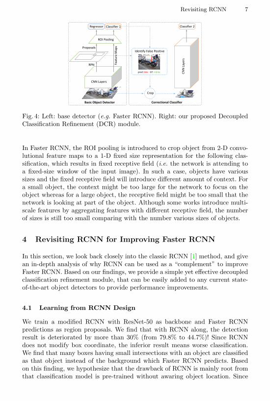
Fig. 4: Left: base detector (e.g. Faster RCNN). Right: our proposed DecoupledClassification Refinement (DCR) module.

In Faster RCNN, the ROI pooling is introduced to crop object from 2-D convo-lutional feature maps to a 1-D fixed size representation for the following clas-sification, which results in fixed receptive field (i.e. the network is attending toa fixed-size window of the input image). In such a case, objects have varioussizes and the fixed receptive field will introduce different amount of context. Fora small object, the context might be too large for the network to focus on theobject whereas for a large object, the receptive field might be too small that thenetwork is looking at part of the object. Although some works introduce multi-scale features by aggregating features with different receptive field, the numberof sizes is still too small comparing with the number various sizes of objects.

4 Revisiting RCNN for Improving Faster RCNN

In this section, we look back closely into the classic RCNN [1] method, and givean in-depth analysis of why RCNN can be used as a “complement” to improveFaster RCNN. Based on our findings, we provide a simple yet effective decoupledclassification refinement module, that can be easily added to any current state-of-the-art object detectors to provide performance improvements.

4.1 Learning from RCNN Design

We train a modified RCNN with ResNet-50 as backbone and Faster RCNNpredictions as region proposals. We find that with RCNN along, the detectionresult is deteriorated by more than 30% (from 79.8% to 44.7%)! Since RCNNdoes not modify box coordinate, the inferior result means worse classification.We find that many boxes having small intersections with an object are classifiedas that object instead of the background which Faster RCNN predicts. Basedon this finding, we hypothesize that the drawback of RCNN is mainly root fromthat classification model is pre-trained without awaring object location. Since


ResNet-50 is trained on ImageNet in multi-crop manner, no matter how muchthe intersection of the crop to the object is, classifier is encouraged to predictthat class. This leads to the classifier in RCNN being “too strong” for proposalclassification, and this is why RCNN needs a carefully tuned sampling strategy,i.e. a ratio of 1:3 of fg to bg. Straightforwardly, we are interested whether RCNNis “strong” enough to correct hard negatives. We make a minor modification tomultiply RCNN classification score with Faster RCNN classification score andobserve a boost of 1.9% (from 79.8% to 81.7%)! Thus, we consider that RCNNcan be seen as a compliment of Faster RCNN in the following sense: the classifierof Faster RCNN is weaker but aware of object location whereas the classifier ofRCNN is unaware of object location but stronger. Based on our findings, wepropose the following three principals to design a better object detector.

Decoupled Features Current detectors still place classification head and lo-calization head on the same backbone, hence we propose that classification headand localization head should not share parameter (as the analysis given in Sec-tion 3), resulted in a decoupled feature using pattern by RCNN.

Decoupled Optimization RCNN also decouples the optimization for objectproposal and classification. In this paper, we make a small change in optimiza-tion. We propose a novel two-stage training where, instead of optimizing the sumof classification and localization loss, we optimize the concatenation of classifi-cation and localization loss, Ldetection = [Lcls + Lbbox, Lcls], where each entry isbeing optimized independently in two steps.

Adaptive Receptive Field The most important advantage of RCNN is that itsreceptive field always covers the whole ROI, i.e. the receptive field size adjustsaccording to the size of the object by cropping and resizing each proposal toa fixed size. We agree that context information may be important for precisedetection, however, we conjuncture that different amount of context introducedby fixed receptive filed might cause different performance to different sizes ofobjects. It leads to our last proposed principal that a detector should an adaptivereceptive field that can change according to the size of objects it attends to. Inthis principal, the context introduced for each object should be proportional toits size, but how to decide the amount of context still remains an open questionto be studied in the future. Another advantage of adaptive receptive field is thatits features are well aligned to objects. Current detectors make predictions athight-level, coarse feature maps usually having a large stride, e.g. a stride of 16or 32 is used in Faster RCNN, due to sub-sampling operations. The sub-samplingintroduces unaligned features, e.g. one cell shift on a feature map of stride 32leads to 32 pixels shift on the image, and defects the predictions. With adaptivereceptive field, the detector always attends to the entire object resulting in analigned feature to make predictions. RCNN gives us a simple way to achieveadaptive receptive field, but how to find a more efficient way to do so remainsan interesting problem needs studying.

Revisiting RCNN 9

4.2 Decoupled Classification Refinement (DCR)

Following these principals, we propose a DCR module that can be easily aug-mented to Faster RCNN as well as any object detector to build a stronger de-tector. The overall pipeline is shown in Fig 4. The left part and the right partare the original Faster RCNN and our proposed DCR module, respectively. Inparticular, DCR mainly consists a crop-resize layer and a strong classifier. Thecrop-resize layer takes two inputs, the original image and boxes produced byFaster RCNN, crops boxes on the original image and feeds them to the strongclassifier after resizing them to a predefined size. Region scores of DCR module(Classifier 2) is aggregated with region scores of Faster RCNN (Classifier 1) byelement-wise product to form the final score of each region. The two parts aretrained separately in this paper and the scores are only combined during testtime.

The DCR module does not share any feature with the detector backbonein order to preserve the quality of classification-aimed translation invariancefeature. Furthermore, there is no error propagation between DCR module andthe base detector, thus the optimization of one loss does not affect the other. Thisin turn results in a decoupled pattern where the base detector is focused moreon localization whereas the DCR module focuses more on classification. DCRmodule introduces adaptive receptive field by resizing boxes to a predefined size.Noticed that this processing is very similar to moving an ROI Pooling from finalfeature maps to the image, however, it is quite different than doing ROI Poolingon feature maps. Even though the final output feature map sizes are the same,features from ROI Pooling sees larger region because objects embedded in animage has richer context. We truncated the context by cropping objects directlyon the image and the network cannot see context outside object regions.

4.3 Training

Since there is no error propagates from the DCR module to Faster RCNN, wetrain our object detector in a two-step manner. First, we train Faster RCNN toconverge. Then, we train our DCR module on mini-batches sampled from hardfalse positives of Faster RCNN. Parameters of DCR module are pre-trained byImageNet dataset [29]. We follow the image-centric method [2] to sample Nimages with a total mini-batch size of R boxes, i.e. R/N boxes per image. Weuse N = 1 and R = 32 throughout experiments. We use a different samplingheuristic that we sample not only foreground and background boxes but also hardfalse positive uniformly. Because we do not want to apply any prior knowledgeto impose unnecessary bias on classifier. However, we observed that boxes fromthe same image have little variance. Thus, we fix Batch Normalization layerwith ImageNet training set statistics. The newly added linear classifier (fullyconnected layer) is set with 10 times of the base learning rate since we want topreserve translation invariance features learned on the ImageNet dataset.


Sample method mAPBaseline 79.8Random 81.8FP Only 81.4FP+FG 81.6FP+BG 80.3FP+FG+BG 82.3RCNN-like 81.7

FP Score mAPBaseline 79.80.20 82.20.25 81.90.30 82.30.35 82.20.40 82.0

Sample size mAPBaseline 79.88 Boxes 82.016 Boxes 82.132 Boxes 82.364 Boxes 82.1

ROI scale mAP Test TimeBaseline 79.8 0.085556 × 56 80.6 0.0525112 × 112 82.0 0.1454224 × 224 82.3 0.5481320 × 320 82.0 1.0465

(a) (b) (c) (d)

DCR Depth mAP Test TimeBaseline 79.8 0.085518 81.4 0.194134 81.9 0.314450 82.3 0.5481101 82.3 0.9570152 82.5 1.3900

Base detector mAPFaster 79.8Faster+DCR 82.3DCN 81.4DCN+DCR 83.2

Model capacity mAPFaster w/ Res101 79.8Faster w/ Res152 80.3Faster Ensemble 81.1Faster w/ Res101+DCR-50 82.3

(e) (f) (g)

Table 1: Ablation studies results. Evaluate on PASCAL VOC2007 test set. Base-line is Faster RCNN with ResNet-101 as backbone. DCR module uses ResNet-50.(a) Ablation study on sampling heuristics. (b) Ablation study on threshold fordefining hard false positives. (c) Ablation study on sampling size. (d) Ablationstudy on ROI scale and test time (measured in seconds/image). (e) Ablationstudy on depth of DCR module and test time (measured in seconds/image). (f)DCR module with difference base detectors. Faster denotes Faster RCNN andDCN denotes Deformable Faster RCNN, both use ResNet-101 as backbone. (g)Comparison of Faster RCNN with same size as Faster RCNN + DCR.

5 Experiments

5.1 Implementation Details

We train base detectors, e.g. Faster RCNN, following their original implementa-tions. We use default settings in 4.3 for DCR module, we use ROI size 224×224and use a threshold of 0.3 to identify hard false positives. Our DCR module isfirst pre-trained on ILSVRC 2012 [29]. In fine-tuning, we set the initial learn-ing rate to 0.0001 w.r.t. one GPU and weight decay of 0.0001. We follow linearscaling rule in [30] for data parallelism on multiple GPUs and use 4 GPUs forPASCAL VOC and 8 GPUs for COCO. Synchronized SGD with momentum 0.9is used as optimizer. No data augmentation except horizontal flip is used.

5.2 Ablation Studies on PASCAL VOC

We comprehensively evaluate our method on the PASCAL VOC detection bench-mark [14]. We use the union of VOC 2007 trainval and VOC 2012 trainval as wellas their horizontal flip as training data and evaluate results on the VOC 2007test set. We primarily evaluate the detection mAP with IoU 0.5 ([email protected]).Unless otherwise stated, all ablation studies are performed with ResNet-50 asclassifier for our DCR module.

Revisiting RCNN 11

Ablation study on sampling heuristic We compare results with differentsampling heuristic in training DCR module:

– random sample: a minibatch of ROIs are randomly sampled for each image– hard false positive only: a minibatch of ROIs that are hard postives are

sampled for each image– hard false positive and background: a minibatch of ROIs that are either hard

postives or background are sampled for each image– hard false positive and foreground: a minibatch of ROIs that are either hard

postives or foreground are sampled for each image– hard false positive, background and foreground: the difference with random

sample heuristic is that we ignore easy false positives during training.– RCNN-like: we follow the Fast RCNN’s sampling heuristic, we sample two

images per GPU and 64 ROIs per image with fg:bg=1:3.

Results are shown in Table 1 (a). We find that the result is insensitive to sam-pling heuristic. Even with random sampling, an improvement of 2.0% in mAPis achieved. With only hard false positive, the DCR achieves an improvement of1.6% already. Adding foreground examples only further gains a 0.2% increase.Adding background examples to false negatives harms the performance by alarge margin of 1.1%. We hypothesize that this is because comparing to falsepositives, background examples dominating in most images results in a classi-fier bias to predicting background. This finding demonstrate the importance ofhard negative in DCR training. Unlike RCNN-like detectors, we do not makeany assumption of the distribution of hard false positives, foregrounds and back-grounds. To balance the training of classifier, we simply uniformly sample fromthe union set of hard false positives, foregrounds and backgrounds. This uniformsample heuristic gives the largest gain of 2.5% mAP. We also compare our train-ing with RCNN-like training. Training with RCNN-like sampling heuristic withfg:bg=1:3 only gains a margin of 1.9%.

Ablation study on other hyperparameters We compare results with dif-ferent threshold for defining hard false positive: [0.2, 0.25, 0.3, 0.35, 0.4]. Resultsare shown in Table 1 (b). We find that the results are quite insensitive to thresh-old of hard false positives and we argue that this is due to our robust uniformsampling heuristic. With hard false positive threshold of 0.3, the performance isthe best with a gain of 2.5%. We also compare the influence of size of sampledRoIs during training: [8, 16, 32, 64]. Results are shown in Table 1 (c). Surpris-ingly, the difference of best and worst performance is only 0.3%, meaning ourmethod is highly insensitive to the sampling size. With smaller sample size, thetraining is more efficient without severe drop in performance.

Speed and accuracy trade-off There are in general two ways to reduce infer-ence speed, one is to reduce the size of input and the other one is to reduce thedepth of the network. We compare 4 input sizes: 56× 56, 112× 112, 224× 224,320×320 as well as 5 depth choices: 18, 34, 50, 101, 152 and their speed. Results


Method mAP aer

o

bik

e

bir

d

boat

bott

le

bu

s

car

cat

chair

cow

tab

le

dog

hors

e

mb

ike

per

son

pla

nt

shee

p

sofa

train

tv

Faster [16] 76.4 79.8 80.7 76.2 68.3 55.9 85.1 85.3 89.8 56.7 87.8 69.4 88.3 88.9 80.9 78.4 41.7 78.6 79.8 85.3 72.0R-FCN [11] 80.5 79.9 87.2 81.5 72.0 69.8 86.8 88.5 89.8 67.0 88.1 74.5 89.8 90.6 79.9 81.2 53.7 81.8 81.5 85.9 79.9SSD [20,21] 80.6 84.3 87.6 82.6 71.6 59.0 88.2 88.1 89.3 64.4 85.6 76.2 88.5 88.9 87.5 83.0 53.6 83.9 82.2 87.2 81.3DSSD [21] 81.5 86.6 86.2 82.6 74.9 62.5 89.0 88.7 88.8 65.2 87.0 78.7 88.2 89.0 87.5 83.7 51.1 86.3 81.6 85.7 83.7

Faster (2fc) 79.8 79.6 87.5 79.5 72.8 66.7 88.5 88.0 88.9 64.5 84.8 71.9 88.7 88.2 84.8 79.8 53.8 80.3 81.4 87.9 78.5Faster-Ours (2fc) 82.5 80.5 89.2 80.2 75.1 74.8 79.8 89.4 89.7 70.1 88.9 76.0 89.5 89.9 86.9 80.4 57.4 86.2 83.5 87.2 85.3

DCN (2fc) 81.4 83.9 85.4 80.1 75.9 68.8 88.4 88.6 89.2 68.0 87.2 75.5 89.5 89.0 86.3 84.8 54.1 85.2 82.6 86.2 80.3DCN-Ours (2fc) 84.0 89.3 88.7 80.5 77.7 76.3 90.1 89.6 89.8 72.9 89.2 77.8 90.1 90.0 87.5 87.2 58.6 88.2 84.3 87.5 85.0

Table 2: PASCAL VOC2007 test detection results.

are shown in Table 1 (d) and (e). The test speed is linearly related to the areaof input image size and there is a severe drop in accuracy if the image size istoo small, e.g. 56× 56. For the depth of classifier, deeper model results in moreaccurate predictions but also more test time. We also notice that the accuracyis correlated with the classification accuracy of classification model, which canbe used as a guideline for selecting DCR module.

Generalization to more advanced object detectors We evaluate the DCRmodule on Faster RCNN and advanced Deformable Convolution Nets (DCN)[13]. Results are shown in Table 1 (f). Although DCN is already among one ofthe most accurate detectors, its classifier still produces hard false positives andour proposed DCR module is effective in eliminating those hard false positives.

Where is the gain coming from? One interesting question is where theaccuracy gain comes from. Since we add a large convolutional network on topof the object detector, does the gain simply comes from more parameters? Or,is DCR an ensemble of two detectors? To answer this question, we compare theresults of Faster RCNN with ResNet-152 as backbone (denoted Faster-152) andFaster RCNN with ResNet-101 backbone + DCR-50 (denoted Faster-101+DCR-50) and results are shown in Table 1 (g). Since the DCR module is simply aclassifier, the two network have approximately the same number of parameters.However, we only observe a marginal gain of 0.5% with Faster-152 while ourFaster-101+DCR-50 has a much larger gain of 2.5%. To show DCR is not simplythen ensemble to two Faster RCNNs, we further ensemble Faster RCNN withResNet-101 and ResNet-152 and the result is 81.1% which is still 1.1% worsethan our Faster-101+DCR-50 model. This means that the capacity does notmerely come from more parameters or ensemble of two detectors.

5.3 PASCAL VOC Results

VOC 2007 We use a union of VOC2007 trainval and VOC2012 trainval fortraining and we test on VOC2007 test. We use the default training setting andResNet-152 as classifier for the DCR module. We train our model for 7 epochsand reduce learning rate by 1

10 after 4.83 epochs. Results are shown in Table 2.

Revisiting RCNN 13

Method mAP aer

o

bik

e

bir

d

boat

bott

le

bu

s

car

cat

chair

cow

tab

le

dog

hors

e

mb

ike

per

son

pla

nt

shee

p

sofa

train

tv

Faster [16] 73.8 86.5 81.6 77.2 58.0 51.0 78.6 76.6 93.2 48.6 80.4 59.0 92.1 85.3 84.8 80.7 48.1 77.3 66.5 84.7 65.6R-FCN [11] 77.6 86.9 83.4 81.5 63.8 62.4 81.6 81.1 93.1 58.0 83.8 60.8 92.7 86.0 84.6 84.4 59.0 80.8 68.6 86.1 72.9SSD [20,21] 79.4 90.7 87.3 78.3 66.3 56.5 84.1 83.7 94.2 62.9 84.5 66.3 92.9 88.6 87.9 85.7 55.1 83.6 74.3 88.2 76.8DSSD [21] 80.0 92.1 86.6 80.3 68.7 58.2 84.3 85.0 94.6 63.3 85.9 65.6 93.0 88.5 87.8 86.4 57.4 85.2 73.4 87.8 76.8

Faster (2fc) 77.3 87.3 82.6 78.8 66.8 59.8 82.5 80.3 92.6 58.8 82.3 61.4 91.3 86.3 84.3 84.6 57.3 80.9 68.3 87.5 71.4Faster-Ours (2fc) 79.9 89.1 84.6 81.6 70.9 66.1 84.4 83.8 93.7 61.5 85.2 63.0 92.8 87.1 86.4 86.3 62.9 84.1 69.6 87.8 76.9

DCN (2fc) 79.4 87.9 86.2 81.6 71.1 62.1 83.1 83.0 94.2 61.0 84.5 63.9 93.1 87.9 87.2 86.1 60.4 84.0 70.5 89.0 72.1DCN-Ours (2fc) 81.2 89.6 86.7 83.8 72.8 68.4 83.7 85.0 94.5 64.1 86.6 66.1 94.3 88.5 88.5 87.2 63.7 85.6 71.4 88.1 76.1

Table 3: PASCAL VOC2012 test detection results.

Method Backbone AP AP50 AP75 APS APM APLFaster (2fc) ResNet-101 30.0 50.9 30.9 9.9 33.0 49.1Faster-Ours (2fc) ResNet-101 + ResNet-152 33.1 56.3 34.2 13.8 36.2 51.5

DCN (2fc) ResNet-101 34.4 53.8 37.2 14.4 37.7 53.1DCN-Ours (2fc) ResNet-101 + ResNet-152 37.2 58.6 39.9 17.3 41.2 55.5

FPN ResNet-101 38.2 61.1 41.9 21.8 42.3 50.3FPN-Ours ResNet-101 + ResNet-152 40.2 63.8 44.0 24.3 43.9 52.6

FPN-DCN ResNet-101 41.4 63.5 45.3 24.4 45.0 55.1FPN-DCN-Ours ResNet-101 + ResNet-152 42.6 65.3 46.5 26.4 46.1 56.4

Table 4: COCO2014 minival detection results.

Notice that based on DCN as base detector, our single DCR module achievesthe new state-of-the-art result of 84.0% without using extra data (e.g. COCOdata), multi scale training/testing, ensemble or other post processing tricks.

VOC 2012 We use a union of VOC2007 trainvaltest and VOC2012 trainvalfor training and we test on VOC2012 test. We use the same training setting ofVOC2007. Results are shown in Table 3. Our model DCN-DCR is the first toachieve over 81.0% on the VOC2012 test set. The new state-of-the-art 81.2% isachieved using only single model, without any post processing tricks.

5.4 COCO Results

All experiments on COCO follow the default settings and use ResNet-152 forDCR module. We train our model for 8 epochs on the COCO dataset and reducethe learning rate by 1

10 after 5.33 epochs. We report results on two different par-tition of COCO dataset. One partition is training on the union set of COCO2014train and COCO2014 val35k together with 115k images and evaluate results onthe COCO2014 minival with 5k images held out from the COCO2014 val. Theother partition is training on the standard COCO2014 trainval with 120k imagesand evaluate on the COCO2015 test-dev. We use Faster RCNN [3], Feature Pyra-mid Networks (FPN) [12] and the Deformable ConvNets [13] as base detectors.

COCO minival Results are shown in Table 4. Our DCR module improvesFaster RCNN by 3.1% from 30.0% to 33.1% in COCO AP metric. Faster RCNNwith DCN is improved by 2.8% from 34.4% to 37.2% and FPN is improved by2.0% from 38.2% to 40.2%. Notice that FPN+DCN is the base detector by top-3


Method Backbone AP AP50 AP75 APS APM APLSSD [20,21] ResNet-101-SSD 31.2 50.4 33.3 10.2 34.5 49.8DSSD513 [21] ResNet-101-DSSD 36.2 59.1 39.0 18.2 39.0 48.2Mask RCNN [31] ResNeXt-101-FPN [32] 39.8 62.3 43.4 22.1 43.2 51.2RetinaNet [33] ResNeXt-101-FPN 40.8 61.1 44.1 24.1 44.2 51.2

Faster (2fc) ResNet-101 30.5 52.2 31.8 9.7 32.3 48.3Faster-Ours (2fc) ResNet-101 + ResNet-152 33.9 57.9 35.3 14.0 36.1 50.8

DCN (2fc) ResNet-101 35.2 55.1 38.2 14.6 37.4 52.6DCN-Ours (2fc) ResNet-101 + ResNet-152 38.1 59.7 41.1 17.9 41.2 54.7

FPN ResNet-101 38.8 61.7 42.6 21.9 42.1 49.7FPN-Ours ResNet-101 + ResNet-152 40.7 64.4 44.6 24.3 43.7 51.9

FPN-DCN ResNet-101 41.7 64.0 45.9 23.7 44.7 53.4FPN-DCN-Ours ResNet-101 + ResNet-152 43.1 66.1 47.3 25.8 45.9 55.3

Table 5: COCO2015 test-dev detection results.

teams in the COCO2017 detection challenge, but there is still an improvementof 1.2% from 41.4% to 42.6%. This observation shows that currently there is noperfect detector that does not produce hard false positives.

COCO test-dev Results are shown in Table 5. The trend is similar to that onthe COCO minival, with Faster RCNN improved from 30.5% to 33.9%, FasterRCNN+DCN improved from 35.2% to 38.1%, FPN improved from 38.8% to40.7% and FPN+DCN improved from 41.7% to 43.1%. We also compare ourresults with recent state-of-the-arts reported in publications and our best modelachieves state-of-the-art result on COCO2015 test-dev with ResNet as backbone.

6 Conclusion

In this paper, we analyze error modes of state-of-the-art region-based objectdetectors and study their potentials in accuracy improvement. We hypothesizethat good object detectors should be designed following three principles: de-coupled features, decoupled optimization and adaptive receptive field. Based onthese principles, we propose a simple, effective and widely-applicable DCR mod-ule that achieves new state-of-the-art. In the future, we will further study whatarchitecture makes a good object detector, adaptive feature representation inmulti-task learning, and efficiency improvement of our DCR module.Acknowledgements. This work is in part supported by IBM-ILLINOIS Centerfor Cognitive Computing Systems Research (C3SR) - a research collaborationas part of the IBM AI Horizons Network; and by the Intelligence AdvancedResearch Projects Activity (IARPA) via Department of Interior/ Interior Busi-ness Center (DOI/IBC) contract number D17PC00341. The U.S. Governmentis authorized to reproduce and distribute reprints for Governmental purposesnotwithstanding any copyright annotation thereon. Disclaimer: The views andconclusions contained herein are those of the authors and should not be inter-preted as necessarily representing the official policies or endorsements, eitherexpressed or implied, of IARPA, DOI/IBC, or the U.S. Government. We thankJiashi Feng for helpful discussions.

Supplementary Materials for Revisiting RCNN:On Awakening the Classification Power of Faster

RCNN

Bowen Cheng1, Yunchao Wei1?, Honghui Shi2,Rogerio Feris2, Jinjun Xiong2, and Thomas Huang1

1University of Illinois at Urbana-Champaign, IL, USA{bcheng9, yunchao, t-huang1}@illinois.edu2IBM T.J. Watson Research Center, NY, USA{Honghui.Shi, rsferis, jinjun}@us.ibm.com

1 Differences with Related Works

RCNN There are two major differences between our DCR module and RCNN.First, our DCR module is an end-to-end classifier. We use softmax classifier ontop of the CNN feature where as RCNN trains another SVM using CNN features.Second, the motivation is different. The purpose of RCNN is to classify eachregion, but the purpose of DCR module is to correct false positives producedby base detectors. The difference in motivation results in different samplingheuristic. RCNN samples a large batch of foreground and background with somefixed ratio to achieve a good balance for training classifier. Our DCR modulenot only samples foreground and background, but also pay attention to samplesthat Faster RCNN makes “ridiculous” mistakes (hard false positives).

Hard Example Selection in Deep Learning Hard example mining is origi-nally used for optimizing SVMs to achieve the global optimum. In [34], an OnlineHard Example Mining (OHEM) algorithm is proposed to train Fast RCNN. In-stead of sampling the minibatch randomly, [34] samples ROIs that have the toplosses (sum of classification and localization loss) with respect to the currentset of parameters. [20] uses a similar online approach, but instead of using hardexamples with largest losses, [20] further imposes a restriction on the ratio offoreground and background in hard examples. The main difference is that hardexamples may not always be hard false positives. DCR module focuses all itsattention to deal with hard false positive which means it is more task-specificthan hard example selection methods. Another difference between OHEM andour approach is that OHEM take both classification and localization loss intoaccount whereas DCR module only considers classification.

Focal Loss (FL) FL [33] is designed to down-weight the loss of well-classifiedexamples by adding an exponential term related to the probability of ground

? corresponding author


truth class, i.e. FL(pt) = −(1 − pt)γ log(pt), where γ is a tunable parameter

specifying how much to down-weight. The motivation of FL is to use a dense setof predefined anchors on all possible image locations without region proposals aswell as the sampling step. Since background dominants in this large set of boxes,FL ends up down-weighting most of losses for backgrounds instead of focusingon hard false positives.

2 More Discussions

Our DCR module demonstrates extremely good performance in suppressing falsepositives. Fig 1 (a) compares total number of false positives on the VOC2007test set. With our DCR module, the number of hard false is reduced by almostthree times (orange). The inference time of DCR module is proportional to thenumber of proposals, input size and network depth. Table 1 (d), (e) compare therunning time and the best model (DCR with depth 152) runs slower than thebaseline Faster RCNN at the speed of 1.39 s/image on 1080 Ti GPU. However,this paper focuses more on the analysis of failure case of object detectors andaccuracy boost, improvement to speed will be studied in the future.

Error Analysis Following [1], we also use the detection analysis tool from [35],in order to gather more information of the error mode of Faster RCNN and DCRmodule. Analysis results are shown in Fig 1.

Fig 1 (a) shows the distribution of top false positive types as scores decrease.False positives are classified into four categories: (1) Loc: IOU with ground truthboxes is in the range of [0.1, 0.5); (2) Sim: detections have at least 0.1 IOU withobjects in predefined similar classes, e.g. dog and cat are similar classes; (3) Oth:detections have at least 0.1 IOU with objects not in predefined similar classes;(4) BG: all other false positives are considered background. We observe thatcomparing with Faster RCNN, DCR module has much larger ratio of localizationerror and the number of false positives is greatly reduced on some classes, e.g. inthe animal class, the number of false positives is largely reduced by 4 times andinitial percentage of localization error increases from less than 30% to over 50%.This statistics are consistent with motivations to reducing classification errorsby reducing number of false positives.

Fig 1 (b) compares the sensitivity of Faster RCNN and DCR to object char-acteristics. [35] defines object with six characteristics: (1) occ: occlusion, wherean object is occluded by another surface; (2) trn: truncation, where there is onlypart of an object; (3) size: the size of an object measure by the pixel area; (4)asp: aspect ratio of an object; (5) view: whether each side of an object is visible;(6) part: whether each part of an object is visible. Normalized AP is used tomeasure detectors performance and more details can be found in [35]. In gen-eral, the higher the normalized AP, the better the performance. The differencebetween max and min value measure the sensibility of a detector, the smallerthe difference, the less sensible of a detector. We observe that DCR improvesnormalized AP and sensitivity on all types of object and improves sensitivity

Supplementary materials 17

significantly on occlusion and size. This increase came from the adaptive field ofDCR, since DCR can focus only on the object area, making it less sensible toocclusion and size of objects.

animals

25 50 100 200 400 800 1600 3200

total false positives

0

10

20

30

40

50

60

70

80

90

100

perc

enta

ge o

f eac

h ty

pe

Loc

Sim

Oth

BG

furniture

25 50 100 200 400 800 1600 3200


0

10

20

30

40

50

60

70

80

90

100

perc

enta

ge o

f eac

h ty

pe

Loc

Sim

Oth

BG

animals

25 50 100 200 400 800 1600 3200


0

10

20

30

40

50

60

70

80

90

100

perc

enta

ge o

f eac

h ty

pe

Loc

Sim

Oth

BG

furniture

25 50 100 200 400 800 1600 3200


0

10

20

30

40

50

60

70

80

90

100

perc

enta

ge o

f eac

h ty

pe

Loc

Sim

Oth

BG

Fast

er

RC

NN

Ou

rs

occ trn size asp view part0

0.2

0.4

0.6

0.8

1Faster RCNN: Sensitivity and Impact

0.504

0.897

0.7840.848

0.524

0.944

0.711

0.887

0.661

0.916

0.711

0.8820.828

occ trn size asp view part0

0.2

0.4

0.6

0.8

1Faster RCNN DCR152: Sensitivity and Impact

0.561

0.907

0.8100.881

0.657

0.947

0.747

0.901

0.716

0.934

0.738

0.9040.859

(a) (b)

Fig. 1: Analysis results between Faster RCNN (top row) and our methods (bot-tom row) by [35]. Left of the dashed line: distribution of top false positive types.Right of the dashed line: sensitivity to object characteristics.

3 Visualization

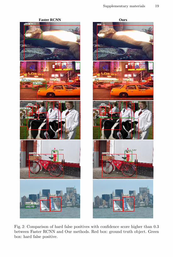
We visualize all false positives with confidence larger than 0.3 for both FasterRCNN and our DCR module in Fig 2. We observe that the DCR module suc-cessfully suppresses all three kinds of hard false positives to some extends.

The first image shows reducing the first type of false positives (part of ob-jects). Faster RCNN (left) classifies the head of the cat with a extremely highconfidence (0.98) but it is eliminated by the DCR module.

The second to the fourth images demonstrate situations of second type of falsepositives (similar objects) where most of false positives are suppressed (“car” inthe second image and “horse” in the third image). However, we find there stillexists some limitations, e.g. the “dog” in the third image where it is supposedto be a cow and the “person” in the fourth image. Although they are not sup-pressed, their scores are reduced significantly (0.96 → 0.38 and 0.92 → 0.52respectively) which will also improve the overall performance. It still remainsan open questions to solve these problems. We hypothesize that by using moretraining data of such hard false positives (e.g. use data augmentation to generatesuch samples).


The last image shows example for the third type of false positives (back-grounds). A part of background near the ground truth is classified as a “boat”by the Faster RCNN and it is successfully eliminated by our DCR module.

References

1. Girshick, R., Donahue, J., Darrell, T., Malik, J.: Rich feature hierarchies for accu-rate object detection and semantic segmentation. In: IEEE CVPR. (2014) 580–587

2. Girshick, R.: Fast r-cnn. In: IEEE ICCV. (2015) 1440–1448

3. Ren, S., He, K., Girshick, R., Sun, J.: Faster r-cnn: Towards real-time objectdetection with region proposal networks. In: NIPS. (2015) 91–99

4. Cai, Z., Vasconcelos, N.: Cascade r-cnn: Delving into high quality object detection.In: IEEE CVPR. (June 2018)

5. Xu, H., Lv, X., Wang, X., Ren, Z., Chellappa, R.: Deep regionlets for objectdetection. arXiv preprint arXiv:1712.02408 (2017)

6. Li, J., Wei, Y., Liang, X., Dong, J., Xu, T., Feng, J., Yan, S.: Attentive contextsfor object detection. IEEE Transactions on Multimedia 19(5) (2017) 944–954

7. Li, J., Liang, X., Li, J., Wei, Y., Xu, T., Feng, J., Yan, S.: Multistage objectdetection with group recursive learning. IEEE Transactions on Multimedia 20(7)(2018) 1645–1655

8. Li, J., Liang, X., Wei, Y., Xu, T., Feng, J., Yan, S.: Perceptual generative adver-sarial networks for small object detection. In: IEEE CVPR. (2017)

9. Liang, X., Liu, S., Wei, Y., Liu, L., Lin, L., Yan, S.: Towards computational babylearning: A weakly-supervised approach for object detection. In: IEEE ICCV.(2015) 999–1007

10. Wei, Y., Shen, Z., Cheng, B., Shi, H., Xiong, J., Feng, J., Huang, T.: Ts2c: Tightbox mining with surrounding segmentation context for weakly supervised objectdetection. In: ECCV. (2018)

11. Dai, J., Li, Y., He, K., Sun, J.: R-fcn: Object detection via region-based fullyconvolutional networks. In: NIPS. (2016) 379–387

12. Lin, T.Y., Dollar, P., Girshick, R., He, K., Hariharan, B., Belongie, S.: Featurepyramid networks for object detection. In: IEEE CVPR. Volume 1. (2017) 4

13. Dai, J., Qi, H., Xiong, Y., Li, Y., Zhang, G., Hu, H., Wei, Y.: Deformable convo-lutional networks. In: IEEE ICCV. (2017) 764–773

14. Everingham, M., Van Gool, L., Williams, C.K.I., Winn, J., Zisserman, A.: Thepascal visual object classes (voc) challenge. IJCV 88(2) (June 2010) 303–338

15. Lin, T.Y., Maire, M., Belongie, S., Hays, J., Perona, P., Ramanan, D., Dollar,P., Zitnick, C.L.: Microsoft coco: Common objects in context. In: ECCV. (2014)740–755

16. He, K., Zhang, X., Ren, S., Sun, J.: Deep residual learning for image recognition.In: IEEE CVPR. (2016) 770–778

17. Uijlings, J.R., Van De Sande, K.E., Gevers, T., Smeulders, A.W.: Selective searchfor object recognition. IJCV 104(2) (2013) 154–171

18. He, K., Zhang, X., Ren, S., Sun, J.: Spatial pyramid pooling in deep convolutionalnetworks for visual recognition. In: ECCV. (2014) 346–361

19. Sermanet, P., Eigen, D., Zhang, X., Mathieu, M., Fergus, R., LeCun, Y.: Overfeat:Integrated recognition, localization and detection using convolutional networks.arXiv preprint arXiv:1312.6229 (2013)

Supplementary materials 19

Faster RCNN Ours

Fig. 2: Comparison of hard false positives with confidence score higher than 0.3between Faster RCNN and Our methods. Red box: ground truth object. Greenbox: hard false positive.


20. Liu, W., Anguelov, D., Erhan, D., Szegedy, C., Reed, S., Fu, C.Y., Berg, A.C.:Ssd: Single shot multibox detector. In: ECCV. (2016) 21–37

21. Fu, C.Y., Liu, W., Ranga, A., Tyagi, A., Berg, A.C.: Dssd: Deconvolutional singleshot detector. arXiv preprint arXiv:1701.06659 (2017)

22. Redmon, J., Divvala, S., Girshick, R., Farhadi, A.: You only look once: Unified,real-time object detection. In: IEEE CVPR. (2016) 779–788

23. Redmon, J., Farhadi, A.: Yolo9000: Better, faster, stronger. In: IEEE CVPR.(2017) 6517–6525

24. Viola, P., Jones, M.J.: Robust real-time face detection. IJCV 57(2) (2004) 137–15425. Freund, Y., Schapire, R.E.: A decision-theoretic generalization of on-line learning

and an application to boosting. Journal of computer and system sciences 55(1)(1997) 119–139

26. Bourdev, L., Brandt, J.: Robust object detection via soft cascade. In: IEEE CVPR.Volume 2. (2005) 236–243

27. Felzenszwalb, P.F., Girshick, R.B., McAllester, D., Ramanan, D.: Object detectionwith discriminatively trained part-based models. IEEE TPAMI 32(9) (2010) 1627–1645

28. Li, H., Lin, Z., Shen, X., Brandt, J., Hua, G.: A convolutional neural networkcascade for face detection. In: IEEE CVPR. (2015) 5325–5334

29. Deng, J., Dong, W., Socher, R., Li, L.J., Li, K., Fei-Fei, L.: Imagenet: A large-scalehierarchical image database. In: IEEE CVPR. (2009) 248–255

30. Goyal, P., Dollar, P., Girshick, R., Noordhuis, P., Wesolowski, L., Kyrola, A., Tul-loch, A., Jia, Y., He, K.: Accurate, large minibatch sgd: training imagenet in 1hour. arXiv preprint arXiv:1706.02677 (2017)

31. He, K., Gkioxari, G., Dollar, P., Girshick, R.: Mask r-cnn. In: IEEE ICCV. (2017)2980–2988

32. Xie, S., Girshick, R., Dollar, P., Tu, Z., He, K.: Aggregated residual transformationsfor deep neural networks. In: IEEE CVPR. (2017) 5987–5995

33. Lin, T.Y., Goyal, P., Girshick, R., He, K., Dollar, P.: Focal loss for dense objectdetection. In: IEEE ICCV. (2017) 2980–2988

34. Shrivastava, A., Gupta, A., Girshick, R.: Training region-based object detectorswith online hard example mining. In: IEEE CVPR. (2016) 761–769

35. Hoiem, D., Chodpathumwan, Y., Dai, Q.: Diagnosing error in object detectors. In:ECCV. (2012) 340–353

Documents

Revisiting RCNN: On Awakening the Classi cation Power of