revised equivalence scale - FRASER

revised equivalence scaleF O R E S T IM A T IN G E Q U IV A L E N T IN C O M E S O R B U D G E T C O S T S B Y F A M IL Y T Y P EB u l le t in No. 1 5 7 0 - 2

U.S. DEPARTMENT OF LABORBUREAU OF LABOR STATISTICS

Digitized for FRASER http://fraser.stlouisfed.org/ Federal Reserve Bank of St. Louis

revised equivalence scaleFOR ESTIMATING EQUIVALENT INCOMES OR BUDGET COSTS BY FAMILY TYPEBulletin No. 1 5 7 0 -2

U.S. DEPARTMENT OF LABOR Willard Wirtz, Secretary BUREAU OF LABOR STATISTICS Ben Burdetsky, Acting Commissioner

November 1968

For sale by the Superintendent of Documents, U.S. Government Printing Office, Washington, D.C., 20402 - Price 35 centsDigitized for FRASER http://fraser.stlouisfed.org/ Federal Reserve Bank of St. Louis


P r e f a c e

Family equivalence scales are measures to determine the relative income required by families differing in composition to maintain equivalent levels of consumption. Ideally, such information would be obtained by developing estimates of budget costs for specified standards of living for various types of families. In lieu of such a battery of family budgets, which would be costly and time-consuming to construct, family equivalence scales have been developed for use with estimated budget costs for a specific type of family to approximate comparable costs for other family types.

Policy decisions and legislation designed to maintain or improve standards of living have multiplied the uses of such equivalence scales. Minimum wages, social security and other social insurance programs, as well as guidelines for public assistance, may be determined on the basis of prescribed levels of adequacy for family living. Programs for college scholarships, for public housing, and for distribution of food through the Food Stamp Plan are among those that attempt to distribute benefits equitably by stipulating family income as a criterion of eligibility.

The intensified attack on poverty after passage of the Economic Opportunity Act of 1964 promptly spotlighted a basic problem facing the Office of Economic Opportunity-defining and identifying the poor. A given income could not indicate comparable well-being for all types of families. Income adequate for an elderly couple fell short of meeting equivalent needs of families with several children.

The Bureau’s Survey of Consumer Expenditures, 1960-61, provided data for calculating new scale values for urban families of different sizes, cross-classified by family composition and age of head. In a sense, the scales introduced in this bulletin may be regarded as a progress report on the continuing program of research being conducted by the Bureau of Labor Statistics (BLS) to measure and evaluate levels of material well-being of American families. A great deal is yet to be known about the consumption behavior of families at different phases of the life cycle. The Bureau’s efforts, as well as research outside the Bureau referred to in appendix D, recognize the need for continued study and review of the assumptions and methods used in deriving equivalence scales.

This bulletin was prepared by Carolyn A. Jackson under the supervision of Helen H. Lamale, Chief of the Division of Living Conditions Studies and Kathryn R. Murphy, Chief of the Branch of Consumer Expenditure Studies. It is one of a series of bulletins prepared under the general direction of Arnold E. Chase, Assistant Commissioner, to report results of the standard budget research program.

m


C o n t e n t s

Page

Concepts and assumptions.................................................................................... 1Formula derivation .............................................................................................. 1Food expenditures-income elasticity ................................................................ 2Steps in deriving scale based on food

expenditures-income......................................................................................... 3Effect of family composition and age of head ................................................ 5Comparison with other scales............................................................................... 7Application of the scale .................................................................................... 9

Costs of goods and services .......................................................................... 9Total budget c o s t s ........................................... 11

Tables:1. Revised equivalence scale for urban families of different size, age,

and composition.................................................................................... 42. Equivalent income scales from selected studies ................................. 83. Estimated annual cost of goods and services for family

consumption at a moderate standard for families of differingsize, type, and age............................................................................... 10

4. Estimated annual cost of a budget providing a moderate livingstandard for families of differing size, type, and age .................... 12

Appendixes:

A. Revised scale of equivalent income before ta x e s ................................. 13Table A-l Revised scale of equivalent income for urban families

of different size, age, and composition ........................................... 14B. Experimentation with food consumption and total consumption

in scale................................................................................................... 15C. Technical references............................................................................... 17D. Research on scales outside the Bureau of Labor Statistics................. 21

Chart:

Revised equivalence scale for selected types of urban families composed of husband, wife, and children .................................................................. 6

iv


R E V I S E D E Q U I V A L E N C E S C A L E : F O R E S T I M A T I N G E Q U I V A L E N T I N C O M E S O R

B U D G E T C O S T S BY F A M I L Y T Y P E

C o n c e p t s a n d A s s u m p t i o n s

The basic problem in deriving an equivalence scale is to obtain an objective means of identifying equivalent levels of consumption for families of varying composition. Research and experimentation with family consumption data accumulated for more than 100 years have resulted in various criteria of general welfare. These include the relative adequacy of diets, the proportion of income spent for various categories of goods, or the proportion of income saved. 1

Historically, a food-income relationship has been the most commonly accepted criterion for appraising levels of living in the United States and in other countries. In 1857, Ernst Engel observed, “The proportion of the outgo used for food, other things being equal, is the best measure of the material standard of living of a population.”* 2

Scales based on a combination of food and nonfood items have been developed, but they have presented more technical difficulties than those based on food alone. The problems arise partly because housing and certain other nonfood expenditures are family rather than individual in character. Prais and Houthakker referred to the difficulties of using nonfood items in scales in terms of the “existence of economies of scale.” This concept “gives expression to the possibility that, with given levels of income per person, a larger household may be able to attain a higher standard of living than a smaller household.” 3 *

In 1948, the BLS presented two scales for measuring equivalent income of families of different sizes with its initial calculation of the City Worker’s Family Budget.4 These BLS scales or relatives of “family well-being” were based on adequacy of diets and amounts of savings. They related only to family size, and did not differentiate by age of head or age of oldest child.

iFor a summary of early consumption scales and source references, see technical reference 26, appendix C. See also technical references 9, 16, and 27. In addition, appendix D contains notes on procedures used outside the Bureau of Labor Statistics in deriving measures of equivalence.

2As translated in Carle C. Zimmerman, Consumption and Standards o f Living, technical reference 27, p. 99, appendix C.

3See appendix D and technical reference 16, pp. 145-146,appendix C.

^Technical reference 23, pp. 28-30 and 49-51, appendix C.

The BLS Survey of Consumer Expenditures in 1950 provided the detailed cross-classification of family expenditures necessary for a scale differentiating six family-size classes by family composition and age of head.5 In that scale, the measure used to determine equivalent income was the proportion of income after taxes spent on food. It is based on the assumption that families spending an equal proportion of income on food have attained an equivalent level of total consumption. The same assumption underlies the revised scale presented here.

Formulation of the equations used for the two latest BLS equivalence scales was preceded by extensive research showing that essentially the same form of relationship between food expenditures and income was observed in eight major consumer expenditure surveys conducted by the BLS between 1888 and 1950.6 Before adopting the 1950 method for the present revision, similar research on the income elasticity of food expenditures was conducted with data from the Survey of Consumer Expenditures, 1960-61.

The principal advantage of the current BLS method of approximating equivalent levels of consumption is its objectivity. It can be calculated directly from measures of actual market behavior of different groups of families. Also, from an operational standpoint, the method is easy to use. It shares limitations of equivalence scales derived by other methods: The assumptions on which they are based are arbitrary and do not take into account all of the factors affecting levels of consumption for families differing in size and stage in the life cycle.

F o r m u l a D e r i v a t i o n

The relatives or indexes of equivalent income for families differing in size, type, and age of head who attained equal levels of consumption were derived from

techn ica l reference 22, appendix C.^Technical reference 3, pp. 149-156, and technical reference

18, pp. 359-393, appendix C.

1Digitized for FRASER http://fraser.stlouisfed.org/ Federal Reserve Bank of St. Louis

the functional relationship of food expenditure and income,7 and expressed by formula:

(1) yi= Ki Cxi)°

Where,

y.= the average expenditure for food by family type i

X|= the average money income after taxes of family type i

Ki= the measure of level of the income-food expenditure relationship for family type i

e= income elasticity of food expenditures, assumed to be approximately

tflThe ratio of food expenditures to income for the i type family,

*i K.— _ —E. (derived by dividing equation (1) by Xj),Xj (x/ 2

when K. ( x ^ 2

K 4 ( x 4 ) 1/2

(2) or x{ K.

K.

2

Before deciding to use this method for revising the scale, the validity of the assumption that the income elasticity of food expenditures was 0.5 was tested with data from the Survey of Consumer Expenditures, 1960-61. Special tabulations also were obtained to experiment with an alternative scale based on the 1960-61 relationship of food consumption and total consumption. This alternative scale is discussed in appendix B.

Food E x p e n d i t u r e s - l n c o m e E l a s t i c i t y

was computed for all urban families and single consumers. It was derived from a regression of the logarithm of average annual food expenditures8 on the logarithm of the average annual money income after taxes for nine income classes, excluding the class “under $ 1,000.” The relationship was linear, and the regression coefficient (or the income elasticity of food expenditure) was 0.53. This figure compares favorably with the elasticity of 0.54 found by previous studies,9 and substantiates the 0.5, or Vi, in the formula used to derive the scale. The value was rounded in the formula to avoid an implication of overprecision and to simplify computations.

Elasticities also were computed for the family types8 shown below:

Deviation in standard

units*

Husband-wife onlyy / = 1.1098 + .5 2 2 7 x '................... 014

Husband-wife, oldest child under 6 years

y ' = 1.0838 + .5 3 2 8 x '................... 045

Husband-wife, oldest child 6-17 years

y / = 1.2714+ .5092X7 ....................020

Husband-wife, oldest child 18 years and older

y '= 1.2310 + .5 1 8 7 x '....................022

One parent-own children only

y ' = .8914 + .5 9 4 8 x '....................018

Single consumer (one person)y '= .5461 + .6 4 9 0 x '....................099

1.62

.73

.45

.83

5.12

1.50

* Assuming universe “e” = 0.5, deviation equals e. . euy ' = log of food expenditures -----------x' = log of money income after taxes £ j~ ei

The income elasticity of food expenditures, or e in formula (1)

y r W

7This is the formula used in deriving the scale based on the 1950 data (see technical reference 22, pp. 1198-1199). For a detailed discussion of the consumption function, see technical references 3 and 18, appendix C.

8Average food expenditures for each income class were adjusted for family size by using an equation which expresses the relationship between the reported family size and the average family size. This empirically derived relationship for standardizing family size was developed by Dorothy S. Brady and Helen A. Barber; see technical reference 2, appendix C.

9Research of Brady and Snyder cited in technical references 3 and 18 showed that income elasticities of food expenditures calculated from over 300 cross-section family expenditure studies in individual cities at different dates yielded an average value of 0.54.


The standard error of the elasticity (a - e^ was highest for one-person families. The income distribution for this family type showed very few persons in the top two classes ($10,000 to $14,999 and $15,000 and over).10 * Averages based on the food expenditures reported by this small number were not considered representative of either the level of food expenditures or the distribution of total food costs between home prepared food and meals in restaurants, etc. for all individuals with incomes of $10,000 or more. Exclusion of the top two income classes from the regression reduced the food elasticity for one-person families to 0.51 and the standard error to 0.033.

The one parent-children family was the only type for which the elasticity (.59) differed significantly (at the 1-percent level) from the Vi or 0.5 assumed in the formula. The relation was linear, and no unusual cases explaining the high regression coefficient could be isolated. H

The algebraic adjustment to the scale to account for the elasticity of income for food being different from that of the base family was computed.12 The effect on the scale results, however, was minor, and for all practical purposes a scale for one-parent families derived in the same manner as for all other types is adequate.

Ste p s in D e r i v i n g S c a l e B a s e d on

F o o d E x p e n d i t u r e s - l n c o m e

To obtain data in the form required for the scale of equivalence represented by equation (2) above, special tabulations from the Survey of Consumer Expenditures,

^Survey o f Consumer Expenditures and Income, 1960-61: Cross-Classification by Family Characteristics, Urban United States, 1960-61, Supplement 2 to BLS Report 237-38, p. 3.

1 !The one-parent families were the smallest group for which a food/income regression was computed. It may he less homogeneous than the other family types since by definition it includes a parent with only grown children, as well as a parent with young children.

12The principal difference in the case where a family-type has an income elasticity for food different from that of the base family is that the equivalent income ratio is no longer a constant but varies with the income of the base family. For example, in the case where the i-th family type has an elasticity of 3/5 the ratio becomes:

x

x4

and it would be necessary to recompute the scale value each year a different budget (i.e., x^) is estimated.

1960-61, were made for urban families. Data were tabulated for each of the four major geographic regions (Northeast, North Central, South, and West) and were combined with population weights to represent the entire urban United States. These tabulations provided average income after taxes and average food expenditures per family for a three-way classification of families13 by: (1) family size, (2) family type, and(3) age of family head. (See table 1.)

The following steps were required to derive the equation of equivalent income x /k \ 2

1. K., or y. (when y = average food expenditure,

( x ^ 2 x = money income after taxesfor ith class) was computed for each size-age-type class.

2. Ratios of K. to K4 for the base class-husband 35 to 44 years, wife, and 2 children, the older 6 to i5 years—were calculated and squared.

3. The squared K ratios for all urban U.S. families were plotted by family type-size for different ages of head and smoothed graphically. Where necessary, lines representing the U.S. were smoothed by averaging regional differences by inspection.

4. A second graphic smoothing was made after plotting the ratios obtained in step 3 by age of head- family type for each size group.

5. The smoothed values for seven age-of-head classes were combined by population weights into four classes, as follows:

Under 35 years (Under 25 and 25 to 34)35 to 54 years (35 to 44 and 45 to 54)55 to 64 years65 years and over (65 to 74 and 75 and over)

The scale values are shown in table !.

13This is the principal difference between the procedures used with 1960-61 and 1950 data. In 1950, three-way classifications were not available. Therefore, an iterative process was used to obtain the three-way classifications from averages for food expenditures and income for each size-age class and each size- type class. In combining the size-age and size-type classes, the

(x )1/2

was assumed to be proportional to Kj on the basis of evidence from the earlier large sample surveys of 1935-36.

3


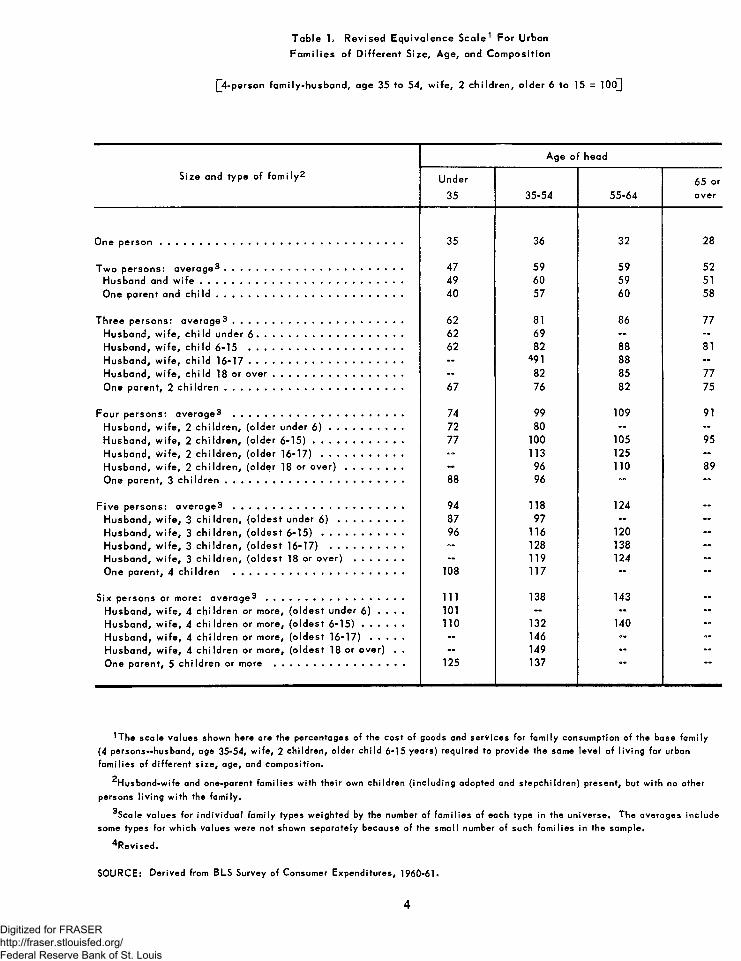
T a b le !« R e v is e d E q u iv a le n c e S c a le 1 F o r U rban

F a m ilie s o f D if fe re n t S ize , A g e , and C o m p o s itio n

|_4-person fa m ily -h u s b a n d , age 35 to 54, w ife , 2 c h ild re n , o ld e r 6 to 15 = 1 0 0 ]

A ge o f head

S ize and ty p e o f fa m ily 2 U nder

35 35-54 55 -64

65 or o ve r

One p e r s o n ..................................................................................................... 35 36 32 28

T w o p e rs o n s : a v e ra g e 3 .......................................................................... 47 59 59 52

H usband and w i f e .................................................................................... 49 60 59 51

One p a re n t and c h i l d .............................................................................. 40 57 60 58

T h re e p e rs o n s : a v e ra g e 3 ....................................................................... 62 81 86 77

H u sb a n d , w ife , c h i ld u n d e r 6 ............................................................. 62 69 — -

H u sb a n d , w ife , c h ild 6 -15 ................................................................ 62 82 88 81

H u sb a n d , w ife , c h ild 1 6 - 1 7 ................................................................ - 4 9 1 88 -

H u sb a n d , w ife , c h ild 18 o r o v e r ...................................................... - 82 85 77

One p a re n t, 2 c h i ld r e n .......................................................................... 67 76 82 75

F o u r p e rs o n s : a v e ra g e 3 ....................................................................... 74 99 109 91

H u sb a n d , w ife , 2 c h ild re n , (o ld e r under 6 ) ............................... 72 80 ~ -

H u sb a n d , w ife , 2 c h ild re n , (o ld e r 6 - 1 5 ) ...................................... 77 100 105 95

H u sb a n d , w ife , 2 c h ild re n , (o ld e r 1 6 - 1 7 ) .................................. — 113 125 —

H u sb a n d , w ife , 2 c h ild re n , (o ld e r 18 or o v e r ) ........................ - 96 no 89

One p a re n t, 3 c h i ld r e n .......................................................................... 88 96 — —

F iv e p e rs o n s : a v e r a g e 3 ....................................................................... 94 118 124 —

H u sb a n d , w ife , 3 c h ild re n , (o ld e s t under 6 ) ........................... 87 97 — —

H u sb a n d , w ife , 3 c h ild re n , (o ld e s t 6 - 1 5 ) .................................. 96 116 120 -

H u sb a n d , w ife , 3 c h ild re n , (o ld e s t 16-17) ............................... 128 138 -

H u sb a n d , w ife , 3 c h ild re n , (o ld e s t 18 or o v e r) ..................... ~ 119 124

One p a re n t, 4 c h ild re n ....................................................................... 108 117 — —

S ix p e rso n s or m ore: a v e ra g e 3 ......................................................... 111 138 143 ~

H u sb a n d , w ife , 4 c h ild re n or m ore, (o ld e s t un der 6) . . . . 101 — — —

H u sb a n d , w ife , 4 c h ild re n or m ore , (o ld e s t 6 -1 5 ) . . . . . . no 132 140 —

H u sb a n d , w ife , 4 c h ild re n o r m ore, (o ld e s t 1 6 - 1 7 ) .............. - 146 - -

H u sb a n d , w ife , 4 c h ild re n or m ore, (o ld e s t 18 or o v e r) . . - 149 - -

One p a re n t, 5 c h ild re n o r more ...................................................... 125 137

^The scale values shown here are the percentages of the cost o f goods and services for fam ily consumption o f the base fam ily

(4 persons— husband, age 35-54, w ife , 2 ch ild ren , older ch ild 6-15 years) required to provide the same level of liv in g for urban

fam ilies of d iffe re n t s ize , age, and com position.

^Husband-w ife and one-parent fam ilies w ith th e ir own ch ildren (inc lud ing adopted and s tepchild ren) present, but w ith no other

persons liv in g w ith the fa m ily .

^Scale values for in d iv id u a l fam ily types weighted by the number o f fa m ilie s of each type in the un iverse. The averages include some types for which values were not shown separately because of the small number of such fam ilies in the sample.

^R evised.

SOURCE: Derived from BLS Survey o f Consumer Expenditures, 1960-61*

4


Effect of F a m i l y C o m p o s i t i o n

a n d A g e of H e a d

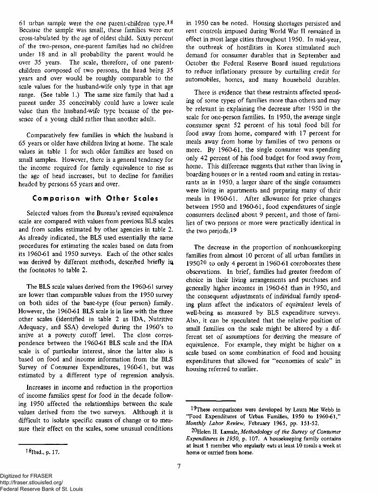
The scale value for each size and type of family in each age class shown in table 1 is expressed as a percent of the spendable income for four-person urban families, composed of husband age 35 to 54 years, wife, and two children, the older of whom is 6 to 15 years old. This general type is most comparable to that described for the City Worker’s Family Budget, which consists of an employed husband 38 years old, his wife, a 13-year old son, and an 8-year old daughter.14 Application of the scale to costs for consumption goods and services in the City Worker’s Family Budget (CWFB) provides estimates of budget costs for consumption goods and services (spendable income) required by different types of urban families. Income and other personal taxes, social security deductions, etc. vary by family size, age, and level of income, and therefore must be calculated separately. An adjusted scale appropriate for application to income before taxes or total budget costs is described in appendix A.

The new scale based on the 1960-61 food expenditure-income relationship confirmed the relationships revealed by the previous BLS scale based on 1950 data. To maintain an equivaient15 level of “well being,” (1) as family size increases, more income is necessary regardless of the family composition and age of head; and, (2) for families with a husband, wife, and children present, income requirements rise as the age of the oldest child increases from under 6 years to 16 or 17 years old.

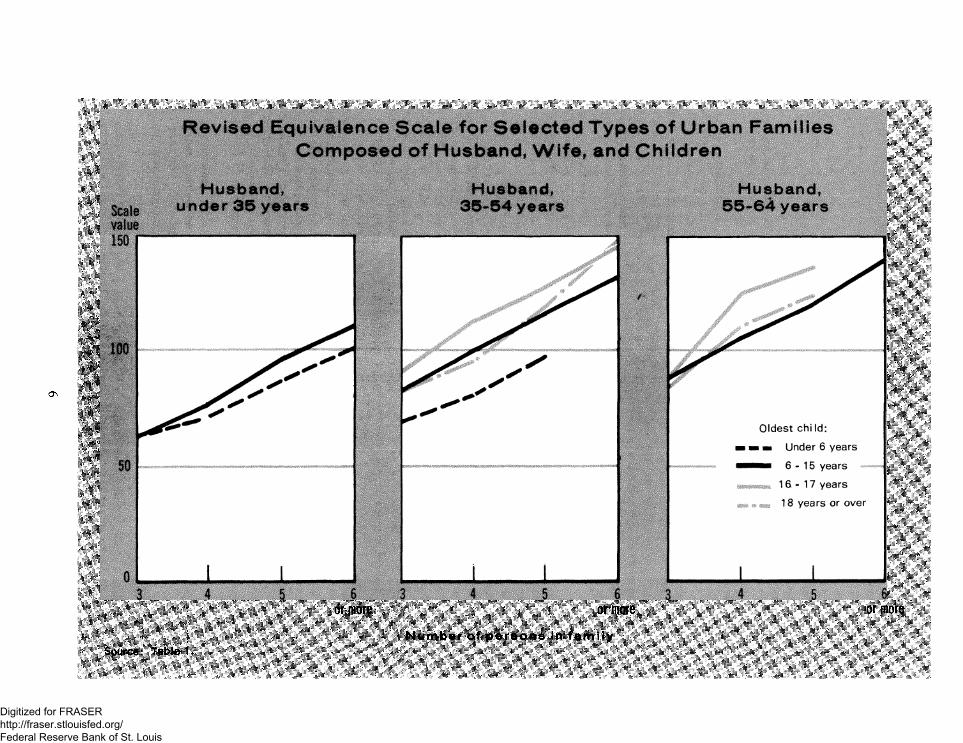
The chart shows that for all husband-wife-children families in which the husband is under 65, the age of the oldest child makes a difference in the income required for the family. Families headed by a husband under 35 are predominantly of two types—the oldest child is 6 to 15 years or is under 6. Although the first type needs more income for all family sizes than the second type, the differences are relatively small. The reason for the similarity may be that in many families having a father under 35 and the oldest child 6 to 15 years, that child is under 12,16 attends elementary

14U.S. Department of Labor, Bureau of Labor Statistics, City Worker’s Family Budget for a Moderate Living Standard, Au- tum 1966 (Bulletin 1570-1).

!5 lt should be kept in mind that equivalent “well being” is measured by the percent of income spent on food.

^Available CES tabulations classify husband-wife families only by the age range of the oldest child and do not show the distribution of children within these age classes.

school, and has not begun the period of rapid growth and the pattern of expenditures associated with teenage youth. A comparison of these young families and the same type families having an older head (35 to 54 years) supports this observation. For all family sizes, the income required for equivalent consumption is higher for the group headed by 35 to 54-year-old fathers than by younger ones. When the father is 35 to 54, probably his oldest child is more frequently 13 to 15 than under 12 years. This 35 to 54 age group, which includes the base- type family, shows most completely the range of changing income requirements as the children grow up.

Families whose oldest son or daughter is 16 or 17 years old in general need more income than other famines; those whose oldest child is 18 years old and over tend to have income requirements similar to families whose oldest child is 6 to 15 years old. Study of the food-income relationships for these groups suggests that although average food expenditures continue to rise for the 18- and -over type, incomes rise faster.

Families having a child 18 and over had higher average incomes and also a higher average number of fulltime earners (1.3 earners) in 1960-61 than any other type of family.17 These data indicate that in a third of the families having a child beyond high school age, not only the father but the mother and/or children were working. If the number of earners had been held constant and, in effect, it was assumed that the children 18 years old or over were dependent on the parent’s income, the decrease in the scale value probably would not have occurred. However, it must be stressed that the data underlying the family equivalence scale had no limitations on employment of family members, such as those specified in the standard budgets for the city worker’s family and the retired couple. The decreasing scale reflects the anomaly that while the presence of children 18 and over adds to the costs for equivalent well-being in some families, these young adults also contribute to the achievement of higher levels of living for the family. On the other hand, food expenditures for the 18-and-over group may have been understated because of difficulties in reporting amounts spent on meals by young people attending school away from home.

The one-parent-children family represents a less homogeneous group than a husband-wife family type specifying the age of the oldest child. Less than 7 percent of the families of two persons or more in the 1960-

17Survey o f Consumer Expenditures, 1960-61: Cross-Classification o f Family Characteristics, Urban United States, 1960- 61, Supplement 2 to BLS Report 237-38, pp. 17-22.

5


or more or more or more

Source: Tablet.Number of p e r s o n s In family


61 urban sample were the one parent-children type. 18 Because the sample was small, these families were not cross-tabulated by the age of oldest child. Sixty percent of the two-person, one-parent families had no children under 18 and in all probability the parent would be over 35 years. The scale, therefore, of one parent- children composed of two persons, the head being 35 years and over would be roughly comparable to the scale values for the husband-wife only type in that age range. (See table 1.) The same size family that had a parent under 35 conceivably could have a lower scale value than the husband-wife type because of the presence of a young child rather than another adult.

Comparatively few families in which the husband is 65 years or older have children living at home. The scale values in table 1 for such older families are based on small samples. However, there is a general tendency for the income required for family equivalence to rise as the age of head increases, but to decline for families headed by persons 65 years and over.

C o m p a r i s o n with O t h e r S c a l e s

Selected values from the Bureau’s revised equivalence scale are compared with values from previous BLS scales and from scales estimated by other agencies in table 2. As already indicated, the BLS used essentially the same procedures for estimating the scales based on data from its 1960-61 and 1950 surveys. Each of the other scales was derived by different methods, described briefly ia the footnotes to table 2.

The BLS scale values derived from the 1960-61 survey are lower than comparable values from the 1950 survey on both sides of the base-type (four person) family. However, the 1960-61 BLS scale is in line with the three other scales (identified in table 2 as IDA, Nutritive Adequacy, and SSA) developed during the 1960’s to arrive at a poverty cutoff level. The close correspondence between the 1960-61 BLS scale and the IDA scale is of particular interest, since the latter also is based on food and income information from the BLS Survey of Consumer Expenditures, 1960-61, but was estimated by a different type of regression analysis.

Increases in income and reduction in the proportion of income families spent for food in the decade following 1950 affected the relationships between the scale values derived from the two surveys. Although it is difficult to isolate specific causes of change or to measure their effect on the scales, some unusual conditions

l 8Ibid.,p. 17.

in 1950 can be noted. Housing shortages persisted and rent controls imposed during World War II remained in effect in most large cities throughout 1950. In mid-year, the outbreak of hostilities in Korea stimulated such demand for consumer durables that in September and October the Federal Reserve Board issued regulations to reduce inflationary pressure by curtailing credit for automobiles, homes, and many household durables.

There is evidence that these restraints affected spending of some types of families more than others and may be relevant in explaining the decrease after 1950 in the scale for one-person families. In 1950, the average single consumer spent 52 percent of his total food bill for food away from home, compared with 17 percent for meals away from home by families of two persons or more. By 1960-61, the single consumer was spending only 42 percent of his food budget for food away from# home. This difference suggests that rather than living in boarding houses or in a rented room and eating in restaurants as in 1950, a larger share of the single consumers were living in apartments and preparing many of their meals in 1960-61. After allowance for price changes between 1950 and 1960-61, food expenditures of single consumers declined about 9 percent, and those of families of two persons or more were practically identical in the two periods. 19

The decrease in the proportion of nonhousekeeping families from almost 10 percent of all urban families in 195020 to only 4 percent in 1960-61 corroborates these observations. In brief, families had greater freedom of choice in their living arrangements and purchases and generally higher incomes in 1960-61 than in 1950, and the consequent adjustments of individual family spending plans affect the indicators of equivalent levels of well-being as measured by BLS expenditure surveys. Also, it can be speculated that the relative position of small families on the scale might be altered by a different set of assumptions for deriving the measure of equivalence. For example, they might be higher on a scale based on some combination of food and housing expenditures that allowed for “economies of scale” in housing referred to earlier. * 2

l^These comparisons were developed by Laura Mae Webb in “Food Expenditures of Urban Families, 1950 to 1960-61,” Monthly Labor Review, February 1965, pp. 151-52.

2®Helen H. Lamale, Methodology o f the Survey o f Consumer Expenditures in 1950, p. 107. A housekeeping family contains at least 1 member who regularly eats at least 10 meals a week at home or carried from home.


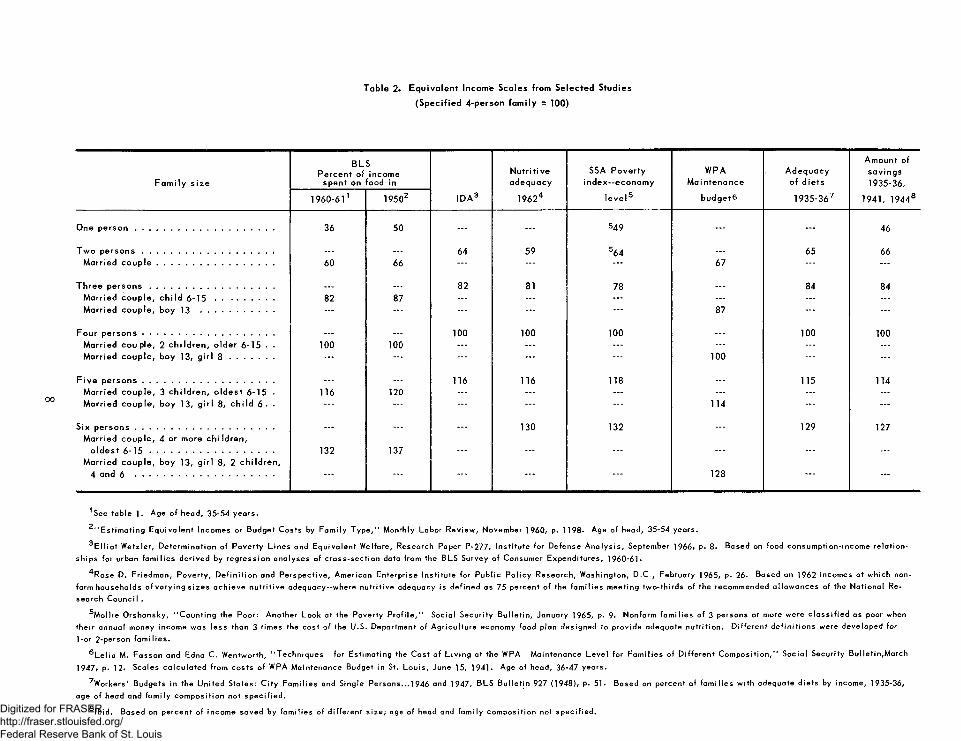
Table 2. E quiva lent Income Scales from Selected Studies

(Specified 4-person fam ily = 100)

Fam i ly s iz e

BLSP e rcen t o f incom e

spen t on food inN u tr it iv eadequacy

SSA P o ve rty index--econom y

WPAM a in tenance

A dequacy o f d ie ts

Am ount of sav ings

1935-36,

1960-61 ' 19502 ID A 3 19624 le v e l5 b u d g e t^ 1935-367 1941, 1944®

One p e r s o n ............................................................... 36 50 . . . . . . 549 . . . . . . 46

T w o p e r s o n s ........................................................ j . . . . . . 64 59 564 . . . 65 66M arried c o u p le ..................................................... 60 66 . . . . . . . . . 67 . . . . . .

T h re e p e r s o n s ......................................................... . . . . . . 82 81 78 . . . 84 84M arried co u p le , c h ild 6 - 1 5 ........................... 82 87 . . . . . . . . . . . . . . . . . .

M arried co u p le , boy 13 ................................. . . . . . . . . . . . . . . . 87 . . . . . .

F our p e r s o n s ............................................................ . . . . . . 100 100 100 . . . 100 100M arried c o u p le , 2 c h ild re n , o ld e r 6 -15 • . 100 100 . . . . . . . . . . . . . . . . . .

M arried c o u p le , boy 13, g ir l 8 .................... . . . . . . . . . . . . . . . 100 . . . . . .

F iv e p ersons ............................................................ . . . . . . 116 116 118 . . . 115 114M arried co u p le , 3 c h ild re n , o ld e s t 6-15 • 116 120 . . . . . . . . . . . . . . . . . .

M a rrie d co u p le , boy 13, g ir l 8, c h ild 6 * * . . . . . . . . . . . . . . . 114 . . . . . .

S ix p ersons ...............................................................M arried co u p le , 4 or more c h ild re n ,

. . . . . . . . . 130 132 . . . 129 127

o ld e s t 6 -15 ........................................................M arried co u p le , boy 13, g ir l 8, 2 c h ild re n ,

132 137 . . . . . . . . . . . . . . . . . .

4 and 6 ............................................................... . . . — 128 .. .

See ta b le 1. A g e o f h e a d , 3 5 -5 4 y e a r s .

^ “ E s t im a t in g E q u iv a le n t In c o m e s o r B u d g e t C o s ts by F a m ily T y p e , ” M o n th ly L a b o r R e v ie w , N o v e m b e r 1 9 6 0 / p* 1198* A g e o f h e a d , 3 5 -5 4 y e a rs .

^ E l l i o t W e tz le r , D e te r m in a t io n o f P o v e r ty L in e s a nd E q u iv a le n t W e lfa re , R e s e a rc h P a p e r P -2 7 7 , I n s t i tu te fo r D e fe n s e A n a ly s is , S e p te m b e r 1 9 6 6 / p . 8 . B a se d on fo o d c o n s u m p tio n - in c o m e r e la t io n

s h ip s fo r u rb a n fa m i lie s d e r iv e d b y re g re s s io n a n a ly s e s o f c ro s s -s e c t io n d a ta fro m th e B L S S u rv e y o f C o n s u m e r E x p e n d itu re s , 1 96 0 -6 1 *

^ R o s e D . F r ie d m a n , P o v e r ty , D e f in i t io n a n d P e r s p e c t iv e , A m e ric a n E n te rp r is e In s t i tu te fo r P u b l ic P o l ic y R e s e a rc h , W a s h in g to n , D „C „, F e b ru a ry 1 9 6 5 , p . 26* B a se d on 196 2 in c o m e s a t w h ic h n o n

fa rm h o u s e h o ld s o f v a ry in g s i ze s a c h ie v e n u t r i t iv e a d e q u a c y --w h e re n u t r i t iv e a d e q u a c y is d e f in e d as 75 p e rc e n t o f th e fa m i lie s m e e tin g tw o - th ird s o f th e re co m m e n d e d a llo w a n c e s o f th e N a t io n a l R e

s e a rc h C o u n c i I .

^ M o l l ie O rs h a n s k y , “ C o u n t in g th e P o o r: A n o th e r L o o k a t th e P o v e rty P r o f i l e , " S o c ia l S e c u r ity B u l le t in , J a n u a ry 1965, p. 9* N o n fa rm fa m i lie s o f 3 p e rs o n s o r m ore w e re c la s s i f ie d as poor w hen

th e ir a n n u a l m o n ey in c o m e w a s le s s th a n 3 t im e s th e c o s t o f th e IL S . D e p a rtm e n t o f A g r ic u l tu r e e c o n o m y fo o d p la n d e s ig n e d to p ro v id e a d e q u a te n u t r i t io n . D i f fe r e n t d e f in i t io n s w e re d e v e lo p e d fo r

1 -o r 2 -p e rs o n fa m i l ie s .

® L e lia M. E a s s o n a nd E dna C„ W e n tw o r th , “ T e c h n iq u e s fo r E s tim a t in g the C o s t o f L iv in g a t th e W PA M a in te n a n c e L e v e l fo r F a m il ie s o f D i f fe r e n t C o m p o s i t io n , " S o c ia l S e c u r ity B u i le t in ,M a r c h

1 9 4 7 , p* 12* S c a le s c a lc u la te d fro m c o s ts o f W PA M a in te n a n c e B u d g e t in S t. L o u is , Ju n e 15, 1 9 4 1 . A g e o f h e a d , 3 6 -4 7 y e a rs .

^ W o rk e rs ’ B u d g e ts in th e U n ite d S ta te s : C i ty F a m il ie s and S in g le P e rs o n s . ..1 9 4 6 and 194 7 , B L S B u l le t in 927 (1 9 4 8 ), p* 5 1. B a s e d on p e rc e n t o f fa m i l ie s w ith a d e q u a te d ie ts by in c o m e , 1 93 5-36 ,

a g e o f h e a d a nd fa m ily c o m p o s it io n n o t s p e c i f ie d .

° l b i d . B a s e d on p e r c e n t o f i n c o m e s a v e d b y f a m i l i e s o f d i f f e r e n t s i z e ; age o f hea d and f a m i l y c o m p o s i t i o n n o t s p e c i f i e d .Digitized for FRASER http://fraser.stlouisfed.org/ Federal Reserve Bank of St. Louis

A p p l i c a t i o n of the S c a l e

Underlying the Revised Equivalence Scale based on the food expenditure-income relationship, as has been stated, is the assumption that families who spend an equal percent of their income on food have attained an equivalent level of consumption. Implicitly the use of this scale also assumes that a family first satisfies its need for food, and then disburses the remaining income for less essential goods and services. Thus, when one family type spends a smaller percent of its income for food than another type, it is assumed that the first family type needs less income to satisfy its food requirement, that is, to provide an equivalent level of consumption.

In general these assumptions are reasonable for most families, but for some family types the percentage of income spent for food may not be an adequate measure of equivalent well-being. Even within the rather narrowly defined family types specified in table 1, there is room for considerable variation in composition and spending patterns, and such variation increases as the number of children and the age of the oldest child rise.21 Also, the scales are based on the market behavior of families as recorded in the Survey of Consumer Expenditures, rather than on standards satisfying specified physical or social requirements. The nature of food expenditures makes them more flexible than those for housing or automobiles that frequently involve longterm obligations, and it may be easier for families to economize on food to offset temporary reductions in income than to reduce contractual payments. Implicitly, the averages on which the scale values are based take account of such variations among families of specified types, but the scales should be used as guidelines and not interpreted in too literal or precise a manner.

The only type of family other than the four-person city worker’s for which BLS has prepared a standard

21 These observations are particularly pertinent in using scale values for the open-end classes of size and age of oldest child. The average number of persons in urban husband and wife families having 4 children or more ranged from 6.1 in families in which all the children were under 6 years to 7.4 persons in families having children 18 and over. The latter group had an average of 3.9 children under 18 and 1.5 children 18 and over. (See CES report cited in footnote 17.) No data were tabulated on the sex or employment status of the children in the CES sample.

budget is the retired couple.22 The U.S. urban average of costs for a retired couple’s budget for a moderate living standard at autumn 1966 prices was 49.6 percent of the costs of goods and services in the budget for the four-person city worker’s family. The Revised Equivalence Scale value for a two-person family in which the husband was 65 years or older was 51 (table 1). The slightly lower percentage indicated by the comparison of standard budgets for the two family types is in the direction that might be expected because the scale value for the couple headed by a husband 65 years or older was derived from family accounts for both employed and retired persons.

Cost of Goods and Services

In using the Revised Equivalence Scale with the City Worker’s Family Budget to estimate the cost of equivalent consumption for other sizes and types of families, the scale values should be applied to the cost of family consumption, i.e., the costs for goods and services. Other outlays or deductions—for income taxes particularly—vary by family size, age of head, and level of income, and must be calculated separately to estimate total budget costs.

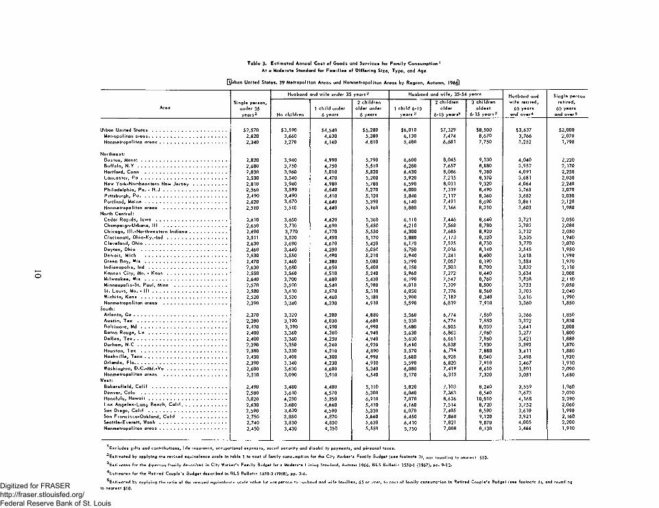
Estimated autumn 1966 costs of goods and services to maintain a moderate living standard for selected types of urban families are shown in table 3. For families headed by persons under 65 years, averages were estimated by applying the Revised Equivalence Scale to the estimated annual cost of consumption in the City Worker’s Family Budget in each of the 39 metropolitan areas and regional groups of nonmetropolitan places for which separate costs were calculated for the CWFB. For the 65 years and older classes, however, the Retired Couple’s Budget is shown for the husband-wife family and has been used as the base for estimating costs for the retired single person. (See footnote 5, table 3.) As indicated in the earlier reference to the Retired Couple’s Budget, these amounts tend to be slightly lower than would be obtained by applying the Revised Equivalence Scale values for the older families to the CWFB. The size and direction of the small differences vary among cities, because the percentage that the Retired Couple’s Budget is of the CWFB varies from city to city.

22Costs of the City Worker’s Family Budget and the Retired Couple’s Budget for a moderate living standard, priced in 39 metropolitan areas and 4 regional classes of nonmetropolitan areas in autumn 1966, and the Revised Equivalence Scale are shown in the 1968 edition of the Bureau’s Handbook o f Labor Statistics (BLS Bulletin 1600).

9


^ r b a n U n ited States, 39 M e tro p o lita n A reas and N o n m e tropo litan A reas by R eg ion , Autum n, 196£]

T a b le 3« E stim ated A nnua l C o s t o f Goods and S e rv ices fo r F a m ily C o n s u m p tio n 1

A t a M oderate Standard fo r F a m ilie s o f D iffe r in g S ize, Type , and Age

AreaS ing le person,

under 35 y e a rs2

H usband and w ife under 35 y e a rs 2 Husband and w ife , 35-54 years Husband and w ife re t ire d ,

65 years and o v e r4

S ing le person re ti red,

65 yearsand overSNo c h ild re n

1 c h ild under 6 years

2 ch ild re n o ld e r under

6 years1 c h ild 6-15

years 2

2 ch i Idren o ld e r

6-15 years3

3 ch ild re n o ld e s t

6-15 y e a rs 2

Urban U n ite d S t a t e s ................................................................. $2,570 $3,590 $4,540 $5,280 $6,010 $7,329 $8,500 $3,637 $2,000M e tro p o lita n a re a s .................................................................... 2,620 3,660 4,630 5,380 6,130 7,474 8,670 3,766 2,070N o n m e tro p o lita n a r e a s .......................................................... 2,340 3,270 4,140 4,810 5,480 6,681 7,750 3,252 1,790

N o rth e a s t:B o s to n , M a s s " . ........................................................................... 2,820 3,940 4,990 5,790 6,600 8,045 9,330 4 ,040 2,220B u ffa lo , N . Y .............................................................................. 2,680 3,750 4,750 5,510 6,280 7,657 8,880 3,952 2,170H a rtfo rd , Conn ....................................................................... 2 ,830 3,960 5,010 5,820 6,630 8,086 9,380 4,091 2,250L a n c a s te r, P a ........................................................................... 2 ,530 3,540 4,470 5,200 5,920 7,215 8,370 3,681 2,030New Y o rk -N o rth e a s te rn New J e r s e y ............................. 2,810 3,940 4,980 5,780 6,590 8,031 9,320 4 ,064 2,240P h ila d e lp h ia , Pa. - N. J ....................................................... 2,560 3,590 4,540 5,270 6,000 7,319 8,490 3,765 2,070P itts b u rg h , P a ............................................................................ 2,490 3,490 4,410 5,120 5,840 7,117 8,260 3,682 2,030P o rtla n d , M a in e ....................................................................... 2,620 3,670 4,640 5,390 6,140 7,491 8,690 3,861 2,120N o n m e tro p o lita n areas ....................................................... 2,510 3,510 4,440 5,160 5,880 7,166 8,310 3,603 1,980

N orth C e n tra l:C edar R a p id s , Iowa ............................................................. 2 ,610 3,650 4,620 5,360 6,110 7,446 8,640 3,721 2,050C ham pa ign -U rbana , I I I ....................................................... 2,650 3,710 4,690 5,450 6,210 7,568 8,780 3,782 2,080C h ica g o , III.-N o rth w e s te rn In d ia n a ................................ 2 ,690 3,770 4,770 5,530 6,300 7,685 8,920 3,732 2,050C in c in n a t i , O h io - K y . - I n d .................................................... 2,511 3,520 4,450 5,170 5,880 7,173 8,320 3,535 1,940C le v e la n d , O hio ....................................................................... 2,630 3,690 4,670 5,420 6,170 7,525 8,730 3,770 2,070D a yton , O hio .......................................................................... 2 ,460 3,440 4,350 5,050 5,750 7,016 8,140 3,545 1,950D e tro it , M ich ....................................................................... 2,530 3,550 4,490 5,210 5,940 7,241 8,400 3,618 1,990Green B ay, W i s ....................................................................... 2 ,470 3,460 4,380 5,080 5,790 7,057 8,190 3,584 1,970In d ia n a p o lis , I n d .................................................................... 2,630 3,680 4,650 5,400 6,150 7,503 8,700 3,832 2,110Kansas C ity , Mo. - K a n s .................................................... 2,550 3,560 4 ,510 5,240 5,960 7,272 8,440 3,634 2,000M ilw a u ke e , Wis ....................................................................... 2,640 3,700 4,680 5,430 6,190 7,547 8,760 3,838 2,110M in n e a p o lis -S t. P a u l, M inn ............................................. 2,570 3,590 4,540 5,280 6,010 7,329 8,500 3,733 2,050St. L o u is , Mo. - I I I ................................................................. 2,580 3,610 4,570 5,310 6,050 7,376 8,560 3,703 2,040W ic h ita , K a n s ........................................................................... 2 ,520 3,520 4,460 5,180 5,900 7,189 8,340 3,616 1,990N o n m e tro p o lita n a reas ....................................................... 2,390 3,340 4,230 4,910 5,590 6,819 7,910 3,360 1,850

South:A tla n ta , G a ................................................................................. 2,370 3,320 4,200 4,880 5,560 6,774 7,860 3,366 1,850A u s t in , T ex .............................................................................. 2,280 3,190 4,030 4,680 5,330 6,774 7,550 3,322 1,830B a lt im o re , M d ........................................................................... 2,420 3,390 4,290 4,990 5,680 6,505 8,030 3,641 2,000B aton R ouge, L a .................................................................... 2,400 3,360 4,260 4,940 5,630 6,863 7,960 3,277 1,800D a lla s , T e x ................................................................................. 2 ,400 3,360 4,250 4,940 5,630 6,861 7,960 3,421 1,880Durham , N - C .............................................................................. 2,390 3,350 4,240 4,920 5,610 6,838 7,930 3,392 1,870H ouston , T ex .......................................................................... 2,380 3,330 4,210 4,890 5,570 6,794 7,880 3,411 1,880N a s h v ille , T e n n ........................................................................ 2,430 3,400 4,300 4,990 5,680 6,928 8,040 3,498 1,920O rla ndo , F la ............................................................. ................... 2,390 3,340 4,230 4,910 5,590 6,820 7,910 3,467 1,910W ash ing ton , D .C . - M d . - V a .................................................... 2,600 3,630 4,600 5,340 6,080 7,419 8,610 3,801 2,090N o n m e tro p o lita n areas ....................................................... 2,210 3,090 3,910 4,540 5,170 6,310 7,320 3,051 1,680

W est:B a k e rs fie ld , C a l if ................................................................. 2,490 3,480 4,400 5,110 5,820 7,103 8,240 3,559 1,960D enver, C o lo ........................................................................... 2,580 3,610 4,570 5,300 6,040 7,363 8,540 3,673 2,020H o n o lu lu , H a w a i i .................................................................... 3,020 4,230 5,350 6,210 7,070 8,626 10,010 4 ,168 2,290Los A n g e le s -L o n g B each, C a l i f ....................................... 2,630 3.680 4,660 5,410 6,160 7,514 8,720 3,752 2,060San D ie g o , C a l if .................................... ............................... 2 ,590 3,630 4,590 5,330 6,070 7,405 8,590 3,610 1,990San F ra n c is c o -O a k la n d , C a l if ....................................... 2,750 3,850 4,870 5,660 6,450 7,860 9,120 3,921 2,160S e a tt le -E v e re tt, W a s h .......................................................... 2,740 3,830 4,850 5,630 6,410 7,821 9,070 4,005 2,200N o n m e tro p o lita n a r e a s .......................................................... 2,450 3,430 4,350 5,550 5,750 7,008 8,130 3,466 1,910

'E x c lu d e s g i f ts and c o n tr ib u t io n s , l i f e in s u ra n c e , oc c u p a tio n a l exp en ses , soc ia l s e c u r ity and d is a b i l i t y paym en ts , and pe rson a l ta x e s .

2 E s tim a te d by a p p ly in g the re v is e d e q u iv a le n c e s ca le in ta b le 1 to c o s t o f fa m ily c on sum p tio n fo r the C ity W orker’ s F a m ily Budget (see fo o tn o te 3 )f and rou nd ing to ne a re s t $10.

^ E s tim a te s fo r the 4-pe rson fa m ily d e s c rib e d in C ity W orker’ s F a m ily Budget for a M oderate L iv in g Standard , Autum n 1966, BLS B u lle t in 1570*1 (1967 ), pp . 9-1 2-

^ E s tim a te s fo r th e R e tire d C o u p le ’ s B u dg e t de scribe d in BLS B u lle t in 1570-3 (1968), pp. 3-6 .

^ E s tim a te d by a p p ly in g the ra tio o f the rev is e d eq u iv a le n c e s ca le v a lue fo r one person to husband and w ife fa m ilie s , 65 or ove r, to c o s t o f fa m ily con sum p tio n in R e tire d C o u p le ’ s B udget (see fo o tn o te 4), and rou nd ing

to ne a re s t $1 0.Digitized for FRASER http://fraser.stlouisfed.org/ Federal Reserve Bank of St. Louis

Total Budget Costs

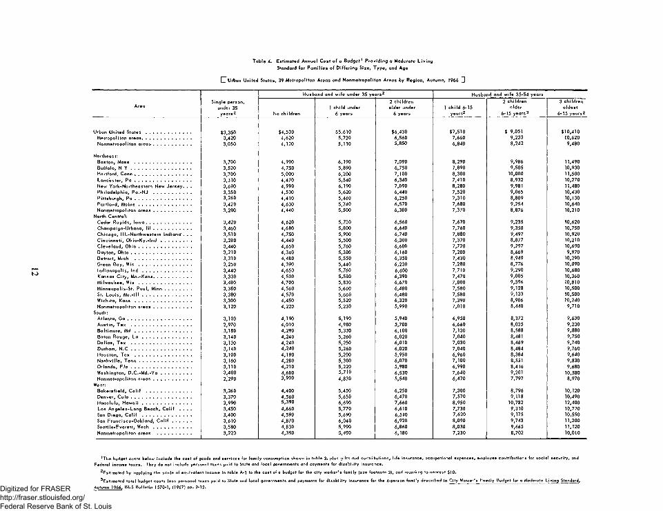
As has been explained, the Revised Equivalence Scale was derived from the relationship of food expenditures to income after personal taxes. For some purposes, however, a scale that more closely approximates total income requirements for different family types is needed. Therefore the BLS has adjusted the Revised Equivalence Scale to include all costs in the CWFB except State and local income taxes and disability insurance. The scale and a statement on its derivation are presented in appendix A. Differences between the two scales are relatively minor. The scale adjusted to measure income before taxes is slightly higher than the Revised Equivalence Scale (table 1) for families of one, two, or three persons, and a little lower for families having five members or more. The direction of these small differences may be attributed to the fact that larger families have more exemptions than smaller families in computing taxes for Federal income tax purposes.

The adjusted scale has been applied to the total budget costs (excluding State and local personal taxes) for the CWFB in 39 metropolitan areas and four regional

groups of nonmetropolitan areas23 (table 4). This scale is also appropriate to use with family income statistics that are reported generally as total income before taxes, for example, in the decennial censuses and in Current Population Surveys conducted by the Bureau of the Census. Adjusted scale values are not shown for families headed by persons 65 years and over, because in the Retired Couple’s Budget it was assumed that most of the income taxes, deductions for social security, etc., were not applicable for older families at a moderate living standard. 2

2 3 In 11 of these areas, such taxes either were not collected or only in nominal amounts (less than $10). In the remaining areas, these taxes represented a small fraction of the total budget costs but estimating the amounts for different family types would be time consuming and difficult, particularly in metropolitan areas including several tax jurisdictions such as Washington, D.C.-Va.-Md. Payments for disability insurance included in the CWFB were applicable only in the States of California, New York, and New Jersey. Users needing more precise budget costs for different family types within a particular area may derive their own estimates of these taxes from local tax sources.


CT Urban U n ited S ta tes, 39 M e tro p o lita n A reas and N on m e tro p o lita n A reas by R egion, Autum n, 1966 U

T a b le 4. E s tim a ted A nnua l C o s t o f a B u d g e t1 P ro v id in g a M oderate L iv in g

Standard fo r F a m ilie s o f D iffe r in g S ize, T ype , and Age

AreaS ing le person,

under 35 y e a rs 2

Husbiand and w ife under 35 y e a rs 2 Husband and w ife 35-54 years

No ch i Idren1 c h ild under

6 years

2 c h ild re n o ld e r under

6 years1 c h ild 6-15

years2

2 ch i Idren o ld e r

6-15 y e a rs 3

3 ch ild re n o ld e s t

6-15 y e a rs 2

Urban U n ite d S t a t e s ....................................... $3,350 $4,530 $5,610 $6,430 $7,510 $ 9,051 $10,410M e tro p o lita n a re a s ........................................... 3,420 4,620 5,720 6,560 7,660 9,233 10,620N o n m e tro p o lita n a r e a s ................................. 3,050 4,120 5,110 5,850 6,840 8,242 9,480

N o rth e a s t:B o s to n , M ass ................................................. 3,700 4,990 6,190 7,090 8,290 9,986 11,490B u ffa lo , N Y .................................................... 3,520 4,750 5,890 6,750 7,890 9,505 10,930H a rtfo rd , C o n n ................................................. 3,700 5,000 6,200 7,100 8,300 10,000 11,500

L a n c a s te r, P a ................................................. 3,310 4,470 5,540 6,340 7,410 8,932 10,270

New Y o rk -N o rth e a s te rn New J e rse y . . . 3,690 4,990 6,190 7,090 8,280 9,981 11,480P h ila d e lp h ia , P a .-N J ................................. 3,350 4,530 5,620 6,440 7,520 9,065 10,430

P itts b u rg h , P a ................................................. 3 ,260 4,410 5,460 6,250 7,310 8,809 10,130P o rtla n d , M a in e .............................................. 3,420 4,630 5,740 6,570 7,680 9,254 10,640N o n m e tro p o lita n a r e a s ................................. 3,280 4,440 5,500 6,300 7,370 8,876 10,210

N orth C e n tra l:Cedar R a p id s , Io w a ....................................... 3 ,420 4,620 5,730 6,560 7,670 9,235 10,620C ham pa ign -U rbana , I I I ................................. 3,460 4,680 5,800 6,640 7,760 9,350 10,750C h ica g o , 111.-N o rth w e s te rn Indiana* . . . 3 ,510 4,750 5,900 6,740 7,880 9,497 10,920C in c in n a t i , O h io - K y . - I n d ........................... 3,280 4 ,440 5,500 6,300 7,370 8,877 10,210

C le v e la n d , O h io .............................................. 3,440 4,650 5,760 6,600 7,720 9,297 10,690

D a yto n , O h io ..................................................... 3 ,210 4,340 5,380 6,160 7,200 8,669 9,970D e tro it , M ich ................................................. 3 ,310 4,480 5,550 6,350 7,430 8,949 10,290Green B ay , W i s .............................................. 3 ,250 4,390 5,440 6,230 7,280 8,776 10,090

In d ia n a p o lis , I n d ........................................... 3 ,440 4,650 5,760 6,600 7,710 9,290 10,680Kansas C ity , M o .-K a n s ................................. 3 ,330 4,500 5,580 6,390 7,470 9,005 10,360M iIw a u ke e , W i s .............................................. 3,480 4 ,700 5,830 6,670 7,800 9,396 10,810

M in n e a p o lis -S t. P a u l, M in n ....................... 3,380 4 ,560 5,660 6,480 7,580 9,128 10,500

3,380 4,570 5,660 6,480 7,580 9,133 10,500

W ic h ita , K a n s ................................................. 3,300 4,450 5,520 6,320 7,390 8,906 10,240

N o n m e tro p o lita n a r e a s ............. ................... 3 ,120 4,220 5,230 5,990 7,010 8,440 9,710

South:A tla n ta , G a ........................................................ 3,100 4,190 5,190 5,940 6,950 8,372 9,630

A u s t in , T e x .................................................... 2,970 4 ,010 4,980 5,700 6,660 8,025 9,230B a lt im o re , M d ................................................. 3,180 4,290 5,330 6,100 7,130 8,588 9,880Baton R ouge, L a ........................................... 3 ,140 4 ,240 5,260 6,020 7,040 8,481 9,750D a lla s , T e x .................................................... 3,130 4 ,240 5,250 6,010 7,030 8,469 9,740D urham , N . C .................................................... 3,140 4 ,240 5,260 6,020 7,040 8,484 9,760H o uston , T ex ................................................. 3 ,100 4,190 5,200 5,950 6 ,960 8,384 9,640N a s h v ille , T e n n .............................................. 3,160 4 ,280 5,300 6,070 7,100 8,551 9,830O rla ndo , F l a ..................................................... 3,110 4,210 5,220 5,980 6,990 8,416 9,680W ash ing ton , D .C . - M d . - V a .......................... 3,400 4,600 5,710 6,530 7,640 9,201 10,580N o n m e tro p o lita n a r e a s ................................. 2,290 3,900 4 ,830 5,540 6,470 7,797 8,970

W est:B a k e rs fie ld , C a l if ....................................... 3 ,260 4,400 5,450 6,250 7,300 8,796 10,120D enver, C o l o .................................................... 3,370 4 ,560 5,650 6,470 7,570 9,118 10,490H o n o lu lu , H a w a i i .......................................... 3,990 5 ,390 6,690 7,660 8,950 10,782 12,400Los A n g e le s -L o n g B each , C a l if . . . . 3,450 4 ,660 5,770 6,610 7,730 9,310 10,710San D iego , C a l if ........................................... 3,400 4 ,590 5,690 6,510 7,620 9,175 10,550San F ra n c is c o -O a k la n d , C a l i f ................. 3,610 4 ,870 6,040 6,920 8,090 9,743 11,200S e a tt le -E v e re tt, W a s h ................................. 3,580 4,830 5,990 6,860 8,030 9,665 11,120

N o n m e tro p o lita n areas .............................. 3 ,220 4 ,350 5,400 6,180 7,230 8,702 10,010

1T he bu dg et c o s ts be lo w in c lu d e the c o s t o f goods and s e rv ic e s fo r fa m ily consum ption show n in ta b le 3, p lus g i f ts and c o n tr ib u te

F ed era l incom e ta x e s . T he y do no t in c lu d e persona l ta xes pa id to State and lo c a l governm ents and paym ents fo r d is a b il i t y in su ran ce ,

l i f e in s u ra n c e , o c c u p a tio n a l e x p en ses , em p loyee c o n tr ib u tio n s fo r s o c ia l s e c u r ity , and

E s t im a te d by a p p ly in g th e s c a le o f e q u iv a le n t incom e in ta b le A-1 to the c o s t of a bu dg e t fo r the c ity w o rk e r ’ s fa m ily (see fo o tn o te 3), and round ing to ne a re s t $10.

E s t im a te d to ta l budget c o s ts le ss pe rson a l ta xes pa id to State and lo c a l governm ents and paym ents fo r d is a b i l i t y in su ran ce fo r th e 4*person fa m ily d e s c rib e d in C ity W orker';

Autum n 1966, B LS B u lle t in 1570 -1, (1967) pp . 9 -12.

F a m ily B u dg e t fo r a M oderate L iv in g Standard ,


A p p e n d i x A. R e v i s e d Sc a le of E q u i v a l e n t Income b efo re T a x e s

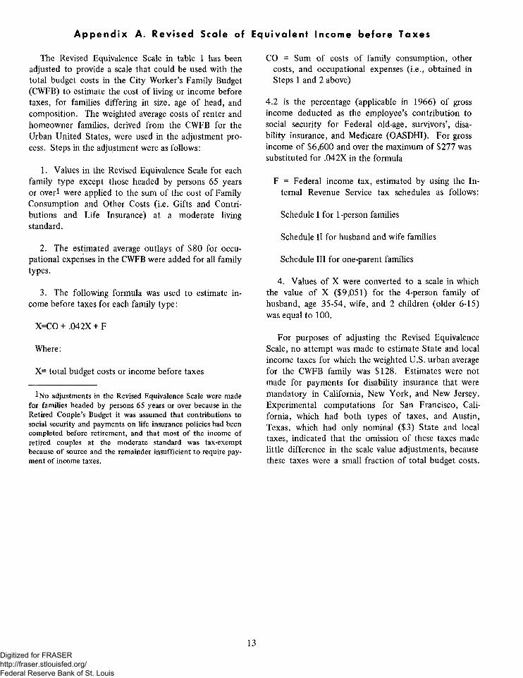
The Revised Equivalence Scale in table 1 has been adjusted to provide a scale that could be used with the total budget costs in the City Worker’s Family Budget (CWFB) to estimate the cost of living or income before taxes, for families differing in size, age of head, and composition. The weighted average costs of renter and homeowner families, derived from the CWFB for the Urban United States, were used in the adjustment process. Steps in the adjustment were as follows:

1. Values in the Revised Equivalence Scale for each family type except those headed by persons 65 years or overl were applied to the sum of the cost of Family Consumption and Other Costs (i.e. Gifts and Contributions and Life Insurance) at a moderate living standard.

2. The estimated average outlays of $80 for occupational expenses in the CWFB were added for all family types.

3. The following formula was used to estimate income before taxes for each family type:

X=CO + .042X + F

Where:

X= total budget costs or income before taxes

iN o adjustments in the Revised Equivalence Scale were made for families headed by persons 65 years or over because in the Retired Couple’s Budget it was assumed that contributions to social security and payments on life insurance policies had been completed before retirement, and that most of the income of retired couples at the moderate standard was tax-exempt because of source and the remainder insufficient to require payment of income taxes.

CO = Sum of costs of family consumption, other costs, and occupational expenses (i.e., obtained in Steps 1 and 2 above)

4.2 is the percentage (applicable in 1966) of gross income deducted as the employee’s contribution to social security for Federal old-age, survivors’, disability insurance, and Medicare (OASDHI). For gross income of $6,600 and over the maximum of $277 was substituted for .042X in the formula

F = Federal income tax, estimated by using the Internal Revenue Service tax schedules as follows:

Schedule I for 1-person families

Schedule II for husband and wife families

Schedule III for one-parent families

4. Values of X were converted to a scale in which the value of X ($9,051) for the 4-person family of husband, age 35-54, wife, and 2 children (older 6-15) was equal to 100.

For purposes of adjusting the Revised Equivalence Scale, no attempt was made to estimate State and local income taxes for which the weighted U.S. urban average for the CWFB family was $128. Estimates were not made for payments for disability insurance that were mandatory in California, New York, and New Jersey. Experimental computations for San Francisco, California, which had both types of taxes, and Austin, Texas, which had only nominal ($3) State and local taxes, indicated that the omission of these taxes made little difference in the scale value adjustments, because these taxes were a small fraction of total budget costs.


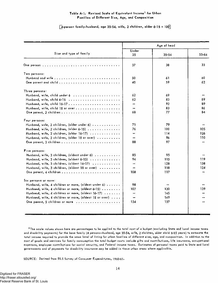
T a b le A - l . R e v is e d S ca le o f E q u iv a le n t In c o m e 1 fo r U rban

F a m ilie s o f D if fe re n t S ize , A g e , and C o m p o s itio n

|~4-person fa m ily -h u s b a n d , age 3 5 -5 4 , w ife , 2 c h ild re n , o ld e r 6 -1 5 = 10(Q

A ge o f head

S ize and ty p e o f fa m ilyU nder

35 35-54 55-64

One p e r s o n ............................................................................................................ 37 38 33

T w o p e rs o n s :

H usba nd and w i f e ........................................................................................... 50 61 60

One p a re n t and c h i l d ..................................................................................... 40 59 62

T h re e p e rs o n s :

H u sb a n d , w ife , c h ild un d e r 6 ................................................................ 62 69 -

H u sb a n d , w ife , c h ild 6 -15 ....................................................................... 62 83 89

H u sb a n d , w ife , c h ild 1 6 - 1 7 ....................................................................... - 92 89

H u sb a n d , w ife , c h ild 18 or o v e r ............................................................. - 83 86

One p a re n t, 2 c h i ld r e n ................................................................................. 68 77 84

F o u r p e rs o n s :

H u sb a n d , w ife , 2 c h ild re n , (o ld e r u n der 6 ) ..................................... 71 79 -

H u sb a n d , w ife , 2 c h ild re n , (o ld e r 6 - 1 5 ) ............................................ 76 100 105

H u sb a n d , w ife , 2 c h ild re n , (o ld e r 1 6 - 1 7 ) ......................................... - 114 126

H u sb a n d , w ife , 2 c h ild re n , (o ld e r 18 or o v e r ) ............................... - 96 110

One p a re n t, 3 c h i ld r e n ................................................................................. 88 97 —

F iv e p e rs o n s :

H u sb a n d , w ife , 3 c h ild re n , (o ld e s t un d e r 6 ) .................................. 85 95 -

H u sb a n d , w ife , 3 c h ild re n , (o ld e s t 6 - 1 5 ) ......................................... 94 115 119

H u sb a n d , w ife , 3 c h ild re n , (o ld e s t 16-17) ..................................... - 128 138

H u s b a n d , w ife , 3 c h ild re n , (o ld e s t 18 or o v e r) ........................... - 118 124

One p a re n t, 4 c h i ld r e n ................................................................................. 108 117 —

S ix p e rso n s or m ore:

H u sb a n d , w ife , 4 c h ild re n or m ore, (o ld e s t un der 6 ) ................. 98 - -

H u sb a n d , w ife , 4 c h ild re n or m ore, (o ld e s t 6 - 1 5 ) ........................ 107 130 139

H u sb a n d , w ife , 4 c h ild re n o r m ore, (o ld e s t 1 6 - 1 7 ) .................... - 145 -

H u sb a n d , w ife , 4 c h ild re n or m ore, (o ld e s t 18 or o v e r) . . . . - 149 -

One p a re n t, 5 c h ild re n o r m ore ............................................................. 124 137

1 The sc a le v a lu e s show n here are percen tages to be a p p lie d to the to ta l c o s t o f a budge t (e x c lu d in g S tate and lo c a l incom e ta xe s

and d is a b i l i t y paym ents) fo r the base fa m ily (4 p e rso n s— husband, age 35-54, w ife , 2 c h ild re n , o ld e r c h ild 6 -15 ye a rs ) to e s tim a te the

to ta l incom e re q u ire d to p ro v id e the same le v e l o f l iv in g fo r urban fa m ilie s o f d if fe re n t s iz e , age, and c o m p o s itio n . In a d d it io n to the

c o s t o f goods and s e rv ic e s fo r fa m ily co nsu m p tion the to ta l budget co s ts in c lu d e g if ts and c o n tr ib u tio n s , l i fe in s u ra n c e , o c c u p a tio n a l

e xp e n se s , em ployee c o n tr ib u tio n s fo r s o c ia l s e c u r ity , and F e d e ra l incom e ta x e s . E s tim a te s o f p ersona l ta xe s pa id to S tate and lo ca l

governm ents and o f paym ents fo r d is a b i l i ty in su ra n ce may be added in those urban areas w here a p p lic a b le .

SO U R C E: D e rive d from BLS Survey o f C onsum er E x p e n d itu re s , 1960-61.


A p p e n d i x B.

E x p e r im e n t a t io n with Food C o n s u m p t io n a n d Total C o n s u m p t io n in S c a le

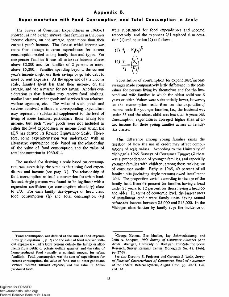
The Survey of Consumer Expenditures in 1960-61 showed, as had earlier surveys, that families in the lower income classes, on the average, spent more than their current year’s income. The class at which income was more than enough to cover expenditures for current consumption varied among family sizes and types. For one-person families it was all after-tax income classes above $2,000 and for families of 2 persons or more, above $5,000. Families spending beyond the current year’s income might use their savings or go into debt to meet current expenses. At the upper end of the income scale, families spent less than their income, on the average, and had a margin for net saving. Another consideration is that famiHes may receive food, clothing, medical care, and other goods and services from relatives, welfare agencies, etc. The value of such goods and services received without a corresponding expenditure may represent a substantial supplement to the level of living of some families, particularly those having low income, but such “free” goods were not included in either the food expenditures or income from which the BLS has derived its Revised Equivalence Scale. Therefore, some experimentation was undertaken with an alternative equivalence scale based on the relationship of the value of food consumption and the value of total consumption in 1960-61.1

The method for deriving a scale based on consumption was essentially the same as that using food expenditures and income (see page 3 ). The relationship of food consumption to total consumption for urban families and single persons was found to be log-linear with a regression coefficient (or consumption elasticity) close to 2/3. For each family size-type-age of head class, food consumption (fj) and total consumption (vj)

iFood consumption was defined as the sum of food expenditures (y in equation 1, p. 2) and the value of food received without expense (i.e., gifts from persons outside the family or allotments from public or private welfare agencies) and the value of home-produced food (usually a nominal amount for urban families). Total consumption was the sum of expenditures for current consumption, the value of food and all other goods and services received without expense, and the value of home- produced food.

were substituted for food expenditures and income, respectively, and the exponent 2/3 replaced Vi in equation (1) and equation (2) as follows:

(3) f, = K,(v/*

<4)A l - l | 3

nvSubstitution of consumption for expenditure/income

averages made comparatively little difference in the scale values for persons living by themselves and for the husband and wife families in which the oldest child was 6 years or older. Values were substantially lower, however, on the consumption scale than on the expenditure/ income scale for younger families, i.e., the husband was under 35 and the oldest child was less than 6 years old. Consumption expenditures averaged higher than aftertax income for these young families across all family- size classes.

This difference among young families raises the question of how the use of credit may affect computations of scale values. According to the University of Michigan’s 1965 Surveys of Consumer Finances,2 there was a preponderance of younger families, and especially younger families with children, among those making use of consumer credit. Early in 1965, 49 percent of all family units (including single persons) owed installment debt. The proportion varied according to the age of the family head from 69 percent for families having a head under 35 years to 12 percent for those having a head 65 and older. In terms of economic level, the largest users of installment credit were family units having annual before-tax income between $5,000 and $15,000. In the Michigan classification by family type the incidence of

2George Katona, Eve Mueller, Jay Schmiedeskamp, and John A. Sonquist, 1965 Survey o f Consumer Finances (Ann Arbor, Michigan, University of Michigan, Institute for Social Research, Survey Research Center, Monograph No. 42, 1966), pp. 27-38.

See also Dorothy S. Projector and Gertrude S. Weiss, Survey o f Financial Characteristics o f Consumers, Board of Governors of the Federal Reserve System, August 1966, pp. 30-31, 126, and 141.

15


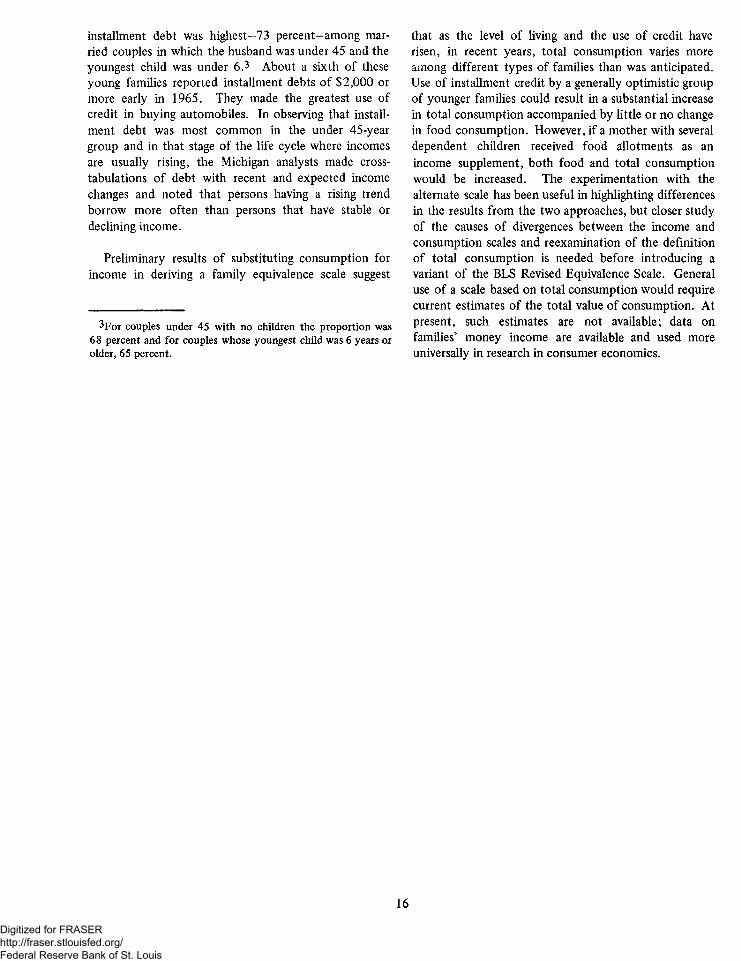
installment debt was highest- 73 percent-among married couples in which the husband was under 45 and the youngest child was under 6.3 About a sixth of these young families reported installment debts of $2,000 or more early in 1965. They made the greatest use of credit in buying automobiles. In observing that installment debt was most common in the under 45-year group and in that stage of the life cycle where incomes are usually rising, the Michigan analysts made crosstabulations of debt with recent and expected income changes and noted that persons having a rising trend borrow more often than persons that have stable or declining income.

Preliminary results of substituting consumption for income in deriving a family equivalence scale suggest

3For couples under 45 with no children the proportion was 68 percent and for couples whose youngest child was 6 years or older, 65 percent.

that as the level of living and the use of credit have risen, in recent years, total consumption varies more among different types of families than was anticipated. Use of installment credit by a generally optimistic group of younger families could result in a substantial increase in total consumption accompanied by little or no change in food consumption. However, if a mother with several dependent children received food allotments as an income supplement, both food and total consumption would be increased. The experimentation with the alternate scale has been useful in highlighting differences in the results from the two approaches, but closer study of the causes of divergences between the income and consumption scales and reexamination of the definition of total consumption is needed before introducing a variant of the BLS Revised Equivalence Scale. General use of a scale based on total consumption would require current estimates of the total value of consumption. At present, such estimates are not available; data on families’ money income are available and used more universally in research in consumer economics.

16


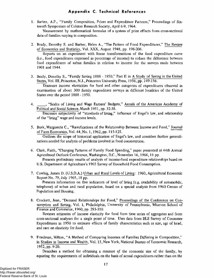
A p p e n d i x C. Techn ica l R e fe r e n c e s

1. Barten, A.P., “Family Composition, Prices and Expenditure Patterns,” Proceedings of Sixteenth Symposium of Colston Research Society, April 6-9,1964.

Measurement by mathematical formulas of a system of price effects from cross-sectional data of families varying in composition.

2. Brady, Dorothy S. and Barber, Helen A., “The Pattern of Food Expenditures,” The Review of Economics and Statistics, Vol. XXX, August 1948, pp. 198-206.

Reports on an experiment with linear transformations of the food expenditure curve (i.e., food expenditures expressed as percentage of income) to reduce the difference between food expenditures of urban families in relation to income for the surveys made between 1901 and 1944.

3. Brady, Dorothy S., “Family Saving 1888 - 1950,” Part II in A Study of Saving in the United States, Vol. Ill, Princeton, N.J., Princeton University Press, 1956, pp. 149-156.

Discusses income elasticities for food and other categories of expenditures observed in examination of about 300 family expenditure surveys in different localities of the United States over the period 1888 - 1950.

4. ____ , “Scales of Living and Wage Earners’ Budgets,” Annals of the American Academy ofPolitical and Social Science, March 1951, pp. 32-38.

Discusses subjectivity of “standards of living,” influence of Engel’s law, and relationship of the “living” wage and income levels.

5. Burk, Marguerite C., “Ramifications of the Relationship Between Income and Food,” Journal of Farm Economics, Vol. 44, No. 1,1962, pp. 115-125.

Outlines the scope of historical application of Engel’s law, and considers further generalizations needed for analysis of problems involved in food consumption.

6. Clark, Faith, “Changing Patterns of Family Food Spending,” paper presented at 44th Annual Agricultural Outlook Conference, Washington, D.C., November 16,1966,11 pp.

Presents preliminary results of analysis of income-food expenditure relationships based on U.S. Department of Agriculture’s 1965 Survey of Household Food Consumption.

7. Cowhig, James D. (U.S.D.A.) Urban and Rural Levels of Living: 1960, Agricultural Economic Report No. 79, July 1965, 18 pp.

Presents information on five indicators of level of living (e.g. availability of automobile, telephone) of urban and rural population, based on a special analysis from 1960 Census of Population and Housing.

8. Crockett, Jean, “Demand Relationships for Food,” Proceedings of the Conference on Con- sumption and Saving, Vol. I, Philadelphia, University of Pennsylvania, Wharton School of Finance and Commerce, 1960, pp. 293-310.

Reviews estimates of income elasticity for food from time series of aggregates and from cross-sectional analyses for a single point of time. Uses data from BLS Survey of Consumer Expenditures in 1950 to estimate effects of family characteristics such as size, age of head, and race on elasticity for food.

9. Friedman, Milton, “A Method of Comparing Incomes of Families Differing in Composition,” in Studies in Income and Wealth, Vol. 15, New York, National Bureau of Economic Research, 1952, pp. 9-20.

Describes a method for obtaining a measure of the economic size of the family, by equating the requirements of individuals on the basis of actual expenditures rather than on the


basis of a standard of need. Uses the food expenditure-income relationship to illustrate the author’s method, but contains a self-critical note on a possibly crucial defect in the method: the basic assumption that a scale of equivalence derived from the food-income relation measures economic welfare.

10. Friedman, Rose D., Poverty Definition and Perspectives, American Enterprise Institute for Public Policy Research, Washington, D.C. February, 1965.

Presents a scale for estimating equivalent income, defined as the income levels at which households of different size achieve adequate nutrition. Derives the income levels (at 1962 prices) from reports from the U.S. Department of Agriculture’s 1955 Household Food Consumption Survey. Defines nutritive adequacy as 75 percent of the families meeting two- thirds of the recommended allowances of the National Research Council.

11. Goldstein, Sidney, Consumption Patterns of the Aged, Philadelphia, University of Pennsylvania, Wharton School of Finance and Commerce, 1960, Chapters IV-VI, pp. 81-100.

Analyzes consumption differences in 1950 with respect to total consumption, food expenditures, and housing expenditures for various ages of family heads.

12. Lamale, Helen H., “Present Day Concepts of Income Adequacy,” presented at 86th Annual Forum of the National Conference on Social Welfare, San Francisco, California, May 28,1959.

Discusses the recent social and economic changes involved in the concept of income adequacy.

13. Manderscheid, Lester V., “Some Observations on Interpreting Measured Demand Elasticities,” Journal of Farm Economics, Vol. 46, February 1964, pp. 128-136.

Relates some of the problems in measuring price and income elasticities to the interpretations of these measures.

14. Orshansky, Mollie, “Counting the Poor: Another Look at the Poverty Profile,” SocialSecurity Bulletin, January 1965, pp. 7-9.

Describes method used to define equivalent incomes at a poverty level for families of different sizes. Bases the scale on food costs for individuals, according to the U.S. Department of Agriculture’s economy food plan at January 1964 prices.

15. Prais, S.J., “The Estimation of Equivalent Adult Scales for Family Budgets,” Economic Journal, December 1953, pp. 791-810.

Presents a method to determine scales of adult equivalents, based on an explicit consumption function. This method was applied to family budgets in the United Kingdom in 1937-38.

16. Prais, S.J. and Houthakker, H.S., The Analysis of Family Budgets, New York, Cambridge University Press, 1955.

Surveys the literature on scales, examines the theory of scales of equivalence, and presents results of a method for analyzing the effects of household composition on consumption as applied to food.

17. Snyder, Eleanor M., “Financing a Family,” Eugenical News, December 1953, pp. 120-129.Summarizes major contributions to research on costs of rearing children in moderate and

higher income families and to the more general analysis of living standards of different groups in the population.

18. -------, “The Impact of Long-term Structural Changes on Family Expenditures: 1888-1950”in Consumer Behavior, New York, Harper and Brothers, 1958, pp. 359-393.

Examines secular changes in consumption functions derived from cross-section surveys of


U.S. urban families from 1888 to 1950. Provides historical detail on values of K (the measure of level of family food expenditures) and of the income elasticities of food expenditures that are basic to BLS estimates of family equivalence scales derived from expenditure surveys for 1950 and 1960-61.

19. _____, Measures of the Dimensions of Poverty in New York City, Hunter College, UrbanResearch Center, June 15,1965.

Presents six selected scales of equivalent incomes by size of family and discusses how the estimated number and distribution of poor families will vary according to the scale used.

20. Stigler, George J., “The Early History of Empirical Studies of Consumer Behavior,” Journal of Political Economy, April 1954, pp. 95-113.

Refers briefly (pp. 101-102) to early applications of income elasticity technique of family budget studies by Del Vecchio (1912) and Ogburn (1919).

21. U.S. Department of Agriculture, Income and Household Size: Their Effects on Food Con- sumption, Marketing Research Report No. 340, June 1959,152 pp.

Uses data from the USDA’s 1955 Household Food Consumption Surveys for extensive computations of elasticities of demand with respect to income for all food and major classes of food, in terms of both quantities of food consumed and value of consumption. Evaluates effects of household size separately.

22. U.S. Department of Labor, Bureau of Labor Statistics, “Estimating Equivalent Incomes or Budget Costs by Family Type,” Monthly Labor Review, November 1960, pp. 1197-1200.

Describes a scale for measuring the relative after-tax income required by families of differing composition to maintain the same level of material well-being, or for estimating comparable costs of goods and services for families of different age, size, and type.

23. _____, Workers’ Budgets in the United States: City Families and Single Persons, 1946 and1947, BLS Bulletin 927,1948, 55 pp.

Presents two separate scales for determining the cost of maintaining families of different size at the same level of material well-being. The scales developed by the BLS for use with its original calculation of the City Worker’s Family Budget were based: (1) on the percentage of families with good or fair diets in terms of nutrition and (2) on the percentage of income al

located to savings.

24. Watts, Harold W., “The Iso-Prop Index: An Approach to the Determination of Differential Poverty Income Thresholds,” Journal of Human Resources, Winter 1967, pp. 2-18.

Describes procedure for constructing an index to measure equivalent levels of poverty for families of varying size in different regions and in urban and rural areas. Uses the share of income devoted to particular categories of consumption as the basis for defining equivalence (e.g. families spending an equal fraction on food or on necessities are considered equally poor). Investigate the properties and suitability of alternative forms of Engel curves and uses data from the BLS Survey of Consumer Expenditures, 1960-61, in regression analysis.

25. Wetzler, Elliot, Determination of Poverty Lines and Equivalent Welfare, Research Paper P-277, Institute for Defense Analyses, September 1966, 23 pp.

Presents results of a study undertaken for Office of Economic Opportunity to construct poverty cut-off levels that take into account size of family, farm/nonfarm differences, and age of the family head. Bases the method for calculating welfare-equivalent income levels on the assumption that families are at equivalent welfare levels when the percentage of their income spent on food is identical. Derives two general types of food-consumption equations by regression analysis from data from the BLS Survey of Consumer Expenditures, 1960-61.


26. Woodbury, Robert Morse, “Economic Consumption Scales and Their Uses,” Journal of American Statistical Association, December 1944, pp. 455-468.

Describes a technique employed by Edgar Sydenstricker and W.I. King in 1921 to develop a consumption scale based on actual expenditures on food and on all items by families of varying composition (in preference to scales having a nutrition or calorie basis) and reviews the direction of research in the 20 years following publication of their study, “The Measurement of the Relative Economic Status of Families.” Contains source references and annotated tables bringing together scales estimated by various methods.

27. Zimmerman, Carle C., Consumption and Standards of Living, New York, Van Nostrand, Co., 1936.

Includes references to early research on scales of adult equivalents in the United States and other countries.


A p p e n d i x D. R e s e a r c h on S c a le s o u ts id e the B u r e a u of L a b o r Statist ics

(N u m b e rs in b r a c k e t s [ ] refer to a p p e n d i x C, T e c h n i c a l R e fe r e n c e s )

Almost all of the numerous equivalence scales cited in the present report or in the technical references listed in appendix C refer to Engel’s work and have used food as the point of departure for estimating equivalent costs. Some have used actual expenditures on food; others, requirements to maintain specified standards of nutritional adequacy. Some, including the BLS scales based on the 1950 and 1960-61 expenditure surveys, have relied primarily or exclusively on a food relationship; others have used food and nonfood expenditures. The extensive quotations that follow have been selected to indicate that in approximately 45 years of research, no consensus has emerged on a method that is objective and operationally practical. The latter consideration probably accounts for the preponderance of scales derived from a food expenditures-income relationship.

Sydenstricker and King published in 19211 “The Measurement of the Relative Economic Status of Families,” which Prais and Houthakker in 1955 [16] characterized as a “fundamental paper.” Referring to these authors Woodbury wrote in 1944 [26]: *

Sydenstricker and King rejected a nutrition or calorie basis for an economic or expenditure scale; and moved in the direction of greater specificity in adopting separate scales for food expenditures, for expenditures on all other items than food and for general expenditures. Their scale for general expenditures was derived from the other two by weighting by the average expenditure on food and all other items. . . .(p. 457)

After reviewing work on expenditure scales in the 20 years since the Sydenstricker-King paper, Woodbury observed [26]:

The paucity of all-items scales is in marked contrast to the relative abundance of new food expenditure scales; the latter reflect the increased attention being paid to diets and parallels the development of specific scales for different nutrients.. . .(pp. 460-61)

An important reason for the paucity of all-items scales on the same level of technical elaboration as those for food and clothing is the tendency observed in a number of recent studies to calculate the number of consumption units in each family, not from the sex and age composition in conjunction with an all-items scale, but as a weighted harmonic average of the number of specific food-expenditure units,

lln Quarterly Publications of the American Statistical Association, Vol. XVII, No. 125, September 1921, pp. 842-57.

clothing-expenditure units and other-items-expenditure units following the procedure first suggested by Kirkpatrick in 1921-22. This method was followed also, for example, in the U.S. Wage Earner Study of 1934-36.2

This technique suggests two important points. First, that all-items scales can be constructed by weighting specific scales for the component elements of the budgets as well as by a direct technique. Secondly, this draws attention immediately to the inequality of coverage of the different elements of the budget: food and clothing are relativelywell covered, but rent and miscellaneous items almost not at all. If these latter enter into the final all-items scale with a weight of approximately 50 percent, the inadequacy of coverage is serious. To these difficulties must be added the further fact that the determination of scale values in the case of expenditures which are family rather than individual in character, such as rent, household expenditures and certain miscellaneous items may involve arbitrary judgments or exclusions.

A second reason for the relative lack of all-items scales lies in the technical difficulties of preparing a new all-items scale in time for use in analyzing the data of the study on which it is based. . . .

Finally, the adoption of the classification according to family type has led to a somewhat lessened emphasis upon all-items scales. 3 The latter have served various purposes, one of which has been to express in numerical relation the demand for consumption goods represented by different family members or additions to the family. But the demand for consumption goods represented by infants or very young children, for example, in families of man, wife and one child can be studied more closely and the results presented more convincingly by an analysis in which families of this type are segregated for examination than by a technique which merely adds their consumption unit value to that of other family members in all types of families. It follows, however, that in the analysis by family type each type group is studied separately, and no attempt is made to summarize or cumulate the results.

When the mass of material permits, detailed study of habits of consumption and expenditure can be made for each important family type; the types chosen are, for example, families with two adults only, families with man, wife and one child, families with man, wife and two to four children,families with man, wife and five or more children, etc..........Obviously, also with the greater degree of specificity in the families selected for study, a larger total mass of material is required to yield a sufficient volume for the detailed groups, (pp. 461-63)

^This reference is to Money Disbursements o f Wage Earners and Clerical Workers, 1934-36, Summary Volume, U.S. Department of Labor, Bureau of Labor Statistics, Bull. 638, pp. 362-66.

^Woodbury’s note: “In the U.S. Consumer Purchases Study, 1935-36, the analysis according to all-items expenditure units was dropped.”

21


Prais and Houthakker in 1955 [16] referred to Woodbury’s survey of economic consumption scales. They presented a method for the analysis of the effects of household composition on consumption and applied the analysis to data from 1937-39 British expenditure surveys to yield scales for six food groups. The following quotations from their “conclusions” and “implications for further research” are similar to Woodbury’s.

Obviously the next step in research along these lines is to obtain comparable estimates for various non-food expenditures; . . .But the straightforward application of the method of this chapter (i.e., 9) would be inadequate for most nonfood items on account of the existence of economies of scale to a significant extent, (p. 145)

The concept of economies of scale gives expression to the possibility that, with given levels of income per person, a larger household may be able to attain a higher standard of living than a smaller household. . . .(p. 146)

As indicated at the beginning of this book, a given piece of research work can hope to fill in only a small portion of anyfield of knowledge................There is, it will be apparent,considerable scope in our case for a synthesis of the various developments presented in the previous chapters which should lead directly to improvements in almost all the estimates presented in this book. The most obvious of these required extensions is the simultaneous estimation of unit- consumer scales and the coefficients of economies of scale so as to bring together the approaches of Chapters 9 and 10. (p. 167)

Prais and Houthakker concluded their extensive analysis with three observations summarized below:

1. Analyses for food commodities have been more successful than those for nonfoods; future research should be directed to bringing analyses for nonfoods to a comparable level.

2. Analyses should begin by grouping nonfood commodities as broadly as possible and then carrying out analyses on successively finer subdivisions.

3. For the successful analysis of the demand for many nonfoods, such as consumers’ durables, reliable information is desirable on current, past, and expected incomes. “Its absence has been at any rate part of the reason for our not taking the inquiries into nonfoods further than we have done and for the relative overattention given to foodstuffs.” (p. 168)

Two recent approaches to finding equivalent levels of income have used data published in BLS reports on the Survey of Consumer Expenditures, 1960-61. (See Wetzler [25] and Watts [24].

Wetzler outlined three alternative techniques generally employed to measure incomes needed to yield equivalent levels of welfare for different groups:

1. Estimate physical needs for one or more commodities (food; or food, clothing, shelter, etc.) of males and females in different age categories, based on standard criteria, and then convert these physical needs into dollars, using market prices to obtain the equivalent dollar need. (Wetzler cited Orshansky’s scale [14] as an example)

2. Use actual expenditures on necessities such as food, or food and clothing, by families of different age and sex composition; calculate expenditures of each family per “consumption unit;” and then classify families into “expenditures-per-consumption-unit” groups.

3. Use the BLS method based on the 1950 CES [22].

Wetzler’s evaluation follows:

. . . Any one of these measures, from a theoretical standpoint, is arbitrary since they all make interpersonal-and intergroup—utility comparisons. From an operational or practical point of view, it is necessary to use a method, preferably simple, which can be generally accepted as giving a good approximation of equivalent levels of welfare.

A good approximation of equivalent levels of welfare appears to be given by the method adopted by the Bureau of Labor Statistics. . . .The BLS method appears to be somewhat less subjective than the first approach. Whereas the first approach tries to make a comparison of welfare which is based on an opinion of physical requirements, the BLS approach is based on the actual market behavior of the groups involved. The main advantage of the BLS method over the second approach is that it is easier to apply in practice, (pp. 2-3)

Wetzler continues with a comparison of the BLS method and the method he used for the Institute of Defense Analysis (IDA):

The method used by IDA to determine equivalent income scales was similar to the BLS method, but differed from it in the following respects:

1. Less restrictive types of equations were used by IDA. The BLS exponent on the income variable was not allowed to vary (being always set equal to Vi) whereas the IDA exponent was permitted to change with family size. In effect, this allowed for variations, which were to be expected, in the percentage change in food consumption associated with a given percentage change in income for different sized families.

2. The IDA equations also permitted estimates to be made, if the need arose, for family types not included in the available data, which was not the case for the BLS or other studies. In other words, IDA equivalent income scales could be derived for any size family (and for any age of head-of-family).

22


3. Since the BLS took average values to determine its coefficients (a’s), it had no numerical estimate of the ‘explanatory power’ of the food-consumption equation it used or of the degree of confidence it could place in the values derived for the a’s. By using regression analysis, it was possible to determine the degree of ‘explanatory power’ of our equations and the amount of confidence that could be placed in our coefficients.” (pp. 3-4)

Watts devised “The Iso-Prop Index” [24] which he explained as:

The name Iso-Prop is an abbreviation for iso-proportional, suggested from the general category of index numbers based on equivalence in terms of the fraction of income (or some other total available for disposition) allocated to a class of expenditures (or subset of possible dispositions), (p. 1)

Watts also reviewed the literature on scales and explained his specific interest in deriving geographic differentials:

In the theoretical and empirical analysis which follows, the Wetzler-BLS-Friedman [25, 22, 9] approach is examined as a method for arriving at geographic differentials. It is probably impossible to give an entirely rigorous or even convincing argument that this procedure adequately reflects all the factors which relate to locational differentials. . . .

The procedure’s most certain advantage lies in its objectivity—it can be calculated directly from measures of observable household behavior as reflected in available data. Its most serious deficiency, in the view of those who prefer to base equivalence on technically prescribed levels of minimum adequacy (e.g., for nutritional intake), is that it may not produce threshold levels which admit the possibility of attaining all such minimum levels, (p. 6)

Watts used published summaries of the CES 1960-61 to carry out regressions for two categories of expenditures: for food and for a group roughly corresponding

to necessities-food, housing, clothing, and transportation. He carried out preliminary regressions using income before tax and income after tax as alternative income measures. The results were quite similar, but only the pre-tax income regressions were reported because they corresponded with the officially recognized Orshansky thresholds of poverty.

In his concluding remarks, Watts stated:

Further empirical work is needed to explore the Iso-Prop Index for inter-city variations. This would provide a more convenient way of graduating the equivalence scales at the borders. For this it would be desirable to use the individual observations from the Consumer Expenditure Survey, instead of the grouped data used here. The city tabulations provide means for income classes or family size classes, but they are not cross-classified.^

In view of the non-constancy of income elasticities,5 it would also be useful to carry out further research on other forms of the Engel curve. When the elasticity is not constant, the income and expenditure data should be deflated by an equivalence index before the relation is estimated. Perhaps an iterative scheme could be used here to obtain successive approximations to an appropriate index, (p. 18)

^Editor’s note: Unpublished cross-tabulations of income after taxes and family size are avaliable for individual cities in the BLS Division of Living Conditions Studies.

5Tests carried out by Watts rejected the hypothesis that income elasticity is constant, (p. 13). It should be noted that this conclusion refers to income elasticities among geographic areas and not among different types of families.

23☆ U.S. GOVERNMENT PRINTING OFFICE : 1968 0 - 3 2 4 -6 7 7
