Embed Size (px)
Citation preview
© C
op
yri
gh
t 2
01
7: In
stitu
to d
e A
stro
no
mía
, U
niv
ers
ida
d N
ac
ion
al A
utó
no
ma
de
Mé
xic
o
Revista Mexicana de Astronomıa y Astrofısica, 53, 385–438 (2017)
Review
THE 2017 RELEASE OF Cloudy
G. J. Ferland1, M. Chatzikos1, F. Guzman1, M. L. Lykins1, P. A. M. van Hoof2, R. J. R. Williams3, N. P.Abel4, N. R. Badnell5, F. P. Keenan6, R. L. Porter7, and P. C. Stancil7
Received May 30 2017; accepted June 28 2017
RESUMEN
Se presenta la version 2017 del codigo de sıntesis espectral Cloudy con mejo-ras en la precision y tratamiento de la fısica hechas desde la version previa. Laexportacion de los datos atomicos hacia bases de datos externas ha permitido laincorporacion de grandes conjuntos de nuevos datos. El uso completo de estos noes practico para la mayorıa de las simulaciones, ası que describimos el subconjuntode datos usado por defecto y que predice un numero considerablemente mayor delıneas que en la version previa. No obstante, la version actual es mas rapida debidoa la optimizacion del codigo. Se dan ejemplos de los lımites de precision de losmodelos pequenos y de los requisitos de rendimiento para los modelos completos.Se resumen avances en los modelos para iones con secuencias isoelectronicas de H yHe y el uso de modelos colisionales-radiativos completos en la determinacion de lasdensidades donde las aproximaciones coronal y de equilibrio termodinamico localfuncionan.
ABSTRACT
We describe the 2017 release of the spectral synthesis code Cloudy, summa-rizing the many improvements to the scope and accuracy of the physics which havebeen made since the previous release. Exporting the atomic data into external datafiles has enabled many new large datasets to be incorporated into the code. The useof the complete datasets is not realistic for most calculations, so we describe the lim-ited subset of data used by default, which predicts significantly more lines than theprevious release of Cloudy. This version is nevertheless faster than the previousrelease, as a result of code optimizations. We give examples of the accuracy limitsusing small models, and the performance requirements of large complete models.We summarize several advances in the H- and He-like iso-electronic sequences anduse our complete collisional-radiative models to establish the densities where thecoronal and local thermodynamic equilibrium approximations work.
Key Words: atomic processes — galaxies: active — methods: numerical — molec-ular processes — radiation mechanisms: general
1University of Kentucky, Lexington, USA.2Royal Observatory of Belgium.3AWE plc, UK.4University of Cincinnati, USA.5University of Strathclyde, Glasgow, UK.6Queen’s University Belfast, Belfast, UK.7University of Georgia, USA.
385
© C
op
yri
gh
t 2
01
7: In
stitu
to d
e A
stro
no
mía
, U
niv
ers
ida
d N
ac
ion
al A
utó
no
ma
de
Mé
xic
o
386 FERLAND ET AL.
CONTENTS
1 INTRODUCTION 386
2 DATABASES 3872.1 The Move to External Databases . . . . . 3872.2 Species and their Names . . . . . . . . . 3882.3 Working with Spectral Lines . . . . . . . 3882.4 Which Database for Which Species? . . . 3892.5 How Complete a Model Should be Done? 3902.6 Generating Reports . . . . . . . . . . . . 391
3 THE IONIZATION EQUILIBRIUM 3923.1 The H- and He-like Iso-electronic Sequences3933.2 A Modified Two-level Approximation for
Other Ions . . . . . . . . . . . . . . . . . . 401
4 ATOMS AND IONS 4074.1 Free-Free Gaunt Factor gIII . . . . . . . 4074.2 Free-Bound Gaunt Factors gII . . . . . . 408
5 THE GRAIN AND CHEMICAL MODELS 4105.1 H2 formation on Grain Surfaces . . . . . 4105.2 H2 Collisions and H2, HD Cooling . . . . 4105.3 How does the PAH Abundance Vary
Across the H+, H0, and H2 Regions of aNebula? . . . . . . . . . . . . . . . . . . . 410
5.4 Lyman Line Pumping in PDR Models . . 4125.5 The LAMDA Database . . . . . . . . . . 4145.6 The Grain Data . . . . . . . . . . . . . . 415
6 THE COOLING FUNCTION 4156.1 Species Cooling . . . . . . . . . . . . . . . 4156.2 Time-Steady Non-Equilibrium Cooling
Function . . . . . . . . . . . . . . . . . . . 4166.3 Time-dependent non-equilibrium cooling . 417
7 OTHER PHYSICS CHANGES 4207.1 Corrections for Isotropic Radiation . . . 4207.2 Chemical Composition . . . . . . . . . . . 4217.3 The Table SED Command and Stellar Grids4217.4 Optical Depth Solution . . . . . . . . . . 422
8 OTHER TECHNICAL CHANGES 4228.1 The Frequency Mesh . . . . . . . . . . . . 4228.2 Grid Runs now fork Multicore . . . . . . 4228.3 Data Layout Optimizations . . . . . . . . 4228.4 Other Changes . . . . . . . . . . . . . . . 4238.5 Online Access . . . . . . . . . . . . . . . 423
APPENDICES
A ATOMIC AND IONIC SPECIES TREATED INCLOUDY 423
B STOUT DATA 423
1. INTRODUCTION
We introduce the next major version of Cloudy,version C17. Cloudy is a non-local thermodynamicequilibrium (NLTE) spectral synthesis and plasma
simulation code designed to simulate astrophysicalenvironments and predict their spectra. The previ-ous version of Cloudy, C13, is described in Fer-land et al. (2013), hereafter referred to as C13, whilethe last major review before C13 was Ferland et al.(1998). These give an overview of the scope andgoals for our simulation code. The basic physics isdescribed in Osterbrock & Ferland (2006), hereafterreferred to as AGN3. Ferland (2003) goes into someatomic and plasma physics questions with examplesof Cloudy applications to photoionized clouds.
A great effort since C13 has gone into movingCloudy’s atomic and molecular data into externaldatabases. These external databases make it possi-ble to compute intensities of a great many emissionlines. A theme running through this review is thetradeoff between the increased accuracy that comesfrom including larger and more complete models,and the associated increase in time and memory. Forthis reason using the full databases is usually notpractical. Command-line user options control thesize of the various model atoms, ions, and molecules.With all databases fully used the number of lines isincreased by well over an order of magnitude, and thedefault setup predicts significantly more lines thanthe previous release. Despite the increased numberof lines, in its default state C17 is actually faster thanC13 because of a good number of optimizations in-troduced to the code base.
The next sections describe how we incorporate anumber of external databases to compute large andcomplex models of ionic and molecular emission. Wethen discuss how we determine the ionization andemission of the gas, and its range of validity. Othermajor changes to the physics and functionality ofthe code are also reviewed. The external data, withits common user interface and underlying software,make it simple to report such quantities as the col-umn density or population in a particular level of aspecies, or its spectrum. We give examples of us-ing Cloudy to compute both equilibrium (Lykinset al. 2013; Wang et al. 2014) and non-equilibrium(Chatzikos et al. 2015) cooling. The former occursif the system has not changed over timescales longerthan those required for atomic processes to reachsteady state. The latter occurs mainly at tempera-tures at or below the 105 K peak in the cooling func-tion, if the temperature changes too rapidly for thesystem to come into ionization equilibrium. Anotherchange includes options to remove isotropic contin-uum sources, such as the CMB, from the spectralpredictions.

© C
op
yri
gh
t 2
01
7: In
stitu
to d
e A
stro
no
mía
, U
niv
ers
ida
d N
ac
ion
al A
utó
no
ma
de
Mé
xic
o
THE 2017 RELEASE OF Cloudy 387
We do not review those parts of the code, its doc-umentation, user support sites, or web access thathave not changed since the release of C13. The C13review paper remains the primary documentation forthose parts of this release.
2. DATABASES
2.1. The Move to External Databases
The greatest effort since C13 has gone into amassive reorganization of our treatment of ions,atoms, or molecules, which we collectively refer toas “species”. Cloudy originally added species mod-els on a case-by-case basis, with the data mixed inwith the source. This was a significant maintenanceproblem since only people with a working knowledgeof C++ could update the data. We have largelymoved the data into external databases. As muchas possible we treat all species with a common codebase. New models are added to our Stout database(Lykins et al. 2015), which was designed to presentdata in formats as close as possible to the originaldata sources, for ease of maintenance.
These databases make it possible to create veryextensive models of line emission that include a verylarge number of levels, although this comes at thecost of longer computing times. They also providethe flexibility of including far fewer levels, with fasterexecution time, but with a less realistic representa-tion of the physics. This compromise between speedand precision will be a theme running throughoutthis review.
There are five distinct databases used to modelspectral lines. These are outlined here and, in moredetail, in later sections.
2.1.1. The H-like and He-like Iso-electronicSequences
We treat atomic one and two electron systems(except H−) with full collisional radiative models,referred to as CRM (see the review by Ferland &Williams 2016). These models are described ingreater detail in § 3.1 below. The models are com-plete, are capable of making highly accurate predic-tions of emission, and go to the interstellar medium(ISM), Local Thermodynamic Equilibrium (LTE)and Strict Thermodynamic Equilibrium (STE) lim-its when appropriate. As described in § 3.2 below,our models of other ions are not as complete.
2.1.2. The H2 Molecule
This, the most common molecule in the universe,is treated as an extensive model introduced in GargiShaw’s thesis (Shaw et al. 2005). Improvements aredescribed in greater detail in § 5 below.
2.1.3. Stout, CHIANTI, and LAMDA Models
We treat emission from atoms, ions, andmolecules (other than those described in the previoussections) using the Stout, CHIANTI, and LAMDAdatabases. These use a common codebase and arecontrolled in very similar ways. The H-like and He-like iso-sequences, and the H2 model, were createdas separate projects and are controlled by a separateset of commands.
For molecules, we use the Leiden Atomic andMolecular Database “LAMDA”8 (Schoier et al.2005). § 5.5 below gives more details. For someions, we use version 7.1.4 of the CHIANTI9 database(Dere et al. 1997; Landi et al. 2012), as described byLykins et al. (2013).
We add new species to our Stout database(Lykins et al. 2015). The data format is designedto be as close as possible to the presentation tablesin the original publications. This makes Stout easyto maintain and update. We use NIST energy levelswhere possible.
The original publications defining the LAMDAand CHIANTI databases should be consulted to findthe original references for individual data sources.Our Stout database is constantly updated. Ap-pendix B gives a summary and references for thedata it uses.
There are many species for which NIST giveslevel energies and transition probabilities but no col-lision data are available. For these we use NIST datawith collision rates from the g-bar approximation(Burgess & Tully 1992). We refer to these as “base-line” models in Appendix B. Lykins et al. (2015) givefurther details.
Baseline model wavelengths should be accurate,and the transition probabilities are matched to theenergy levels, but the g-bar collision strengths arehighly approximate. High-quality collision data areavailable for most astrophysically important species,as shown in Appendix B, so baseline models aremainly used for species that are not commonly ob-served.
There are several considerations to keep in mindif a baseline species is important in a particular ap-plication. First, the collision rates are highly ap-proximate, so at low densities the line intensities willbe too. If the density is high enough for the lev-els to be in LTE the predictions will be fine. How-ever, with some effort, the predictions could be im-proved. First, the OPEN-ADAS data collection10
8http://www.strw.leidenuniv.nl/~moldata/9http://www.chiantidatabase.org/
10http://open.adas.ac.uk/
© C
op
yri
gh
t 2
01
7: In
stitu
to d
e A
stro
no
mía
, U
niv
ers
ida
d N
ac
ion
al A
utó
no
ma
de
Mé
xic
o
388 FERLAND ET AL.
does include plane-wave Born or distorted-wave col-lision rates. These are better than g-bar but the dataset is not matched to NIST energies. This match-ing can be done with some effort, as has been donefor Fe II (Verner et al. 1999) and Si II (Laha et al.2016). Alternatively, members of the atomic physicscommunity could be asked to produce close-couplingcollision rates for the astrophysical application.
Cloudy has long included a large and very com-plete model of Fe II emission which was developedas part of Katya Verner’s thesis (Verner et al. 1999).Modern atomic calculations now routinely providedatasets of similar or larger size, so the current ver-sion of Cloudy can create complex emission modelsof any species with sufficient data. The Verner et al.(1999) Fe II model is now fully integrated into theStout database.
2.2. Species and their Names
Cloudy simulates gas ranging from fully ionizedto molecular. Nomenclature varies considerably be-tween chemical, atomic, and plasma physics. Wehave adopted a naming convention that tries to finda middle ground between these different fields.
A particular atom, ion, or molecule is referredto as a “species”. A species is a baryon, and thisrelease of Cloudy has 625 species. Examples areCO, H2, H
+, and Fe22+. Species are treated using acommon approach, as much as possible. Our namingconvention melds a bit of each of these fields becausea single set of rules must apply to all species.
• Species labels are case sensitive, to distinguishbetween the molecule “CO” and the atom “Co”.
• At present we do not use “_” to indicate sub-scripts, or “^” to indicate charge.
• Molecules are written pretty much as they ap-pear in texts. H2, CO, and H− would be writtenas “H2”, “CO”, and “H-”.
• Atoms are the element symbol by itself. Exam-ples are “H” or “He” and not the atomic physicsnotation H0 or He0.
• Ions are given by “+” followed by the netcharge. Examples are “He+2” or “Fe+22” andnot the correct atomic physics notation, He2+
or Fe22+. The latter would clash with notationfor molecular ions. “C2+” indicates C+
2 in ournotation.
• We specify isotopes using “ˆ” and the atomicweight placed before the atom to which it refers.
For example, “ˆ13CO” is the carbon monoxideisotopologue 13CO.
Appendix B lists our species together with thedatabase used to treat them.
2.3. Working with Spectral Lines
These species may emit a collection of photonswhich we refer to as a spectrum, although the speciesand spectrum may be labeled differently. We followthe spectroscopic convention that a spectral line isidentified by a label and a wavelength. The nextsections discuss how each is specified.
2.3.1. Specifying Spectral Lines
We follow a modified atomic physics notation forthe spectrum. In atomic physics, H I, He II, andC IV are the spectra emitted by H0, He+, and C3+.“H I” indicates a collection of photons while H0 isa baryon. In our notation, we replace the Romannumeral with an integer so we refer to the spec-trum as “H 1” and the baryon as “H” in the output.For example, H I λ4861A, He II λ4686A, and theC IV λ1549A doublet would appear in the output asH 1 4861.36, He 2 4686.01, and Blnd 1549.00 (blendsare discussed below).
Chemistry does not suffer from this distinctionbetween baryons and spectra so the species label isalso the spectroscopic ID. Some examples of molecu-lar lines in the output might include H2O 538.142m,HNC 1652.90m, HCS+ 1755.88m, CO 2600.05m,CO 1300.05m, ˆ13CO 906.599m. In this contextthe “m” indicates microns rather than our defaultangstrom unit.
To summarize, atomic hydrogen would be refer-enced as “H” while the Lα line would be “H 1”.The distinction is important because, depending onwhether it is formed by collisional excitation or re-combination, Lα can trace either H0 or H+.
We continue to follow the spectroscopic conven-tion of denoting a line by its species label and wave-length. This has the problem that several lines ina rich spectrum may have the save wavelength, atleast to our quoted precision. An example is thestrongest molecular hydrogen line that can be mea-sured from the ground. The H2 1-0 S(1) transi-tion has a wavelength of 2.121 µm. However thereare a number of H2 lines with nearly this wave-length; 3-2 S(23) 2.11751µm, 1-0 S(1) 2.12125µm,and 3-2 S(4) 2.12739µm. We ameliorate this confu-sion by reporting the wavelengths with six significantfigures in this version. However, this method of iden-tifying lines is fragile and it is still possible that thecode will find a line with the specified wavelengththat is not the intended target.
© C
op
yri
gh
t 2
01
7: In
stitu
to d
e A
stro
no
mía
, U
niv
ers
ida
d N
ac
ion
al A
utó
no
ma
de
Mé
xic
o
THE 2017 RELEASE OF Cloudy 389
2.3.2. Line Blends
We introduce the concept of “line blends” in thisversion. These have the label “Blnd” in the mainoutput, and a simplified wavelength. An example isBlnd 2.12100m, which is the sum of the three H2
lines mentioned above. Operationally, a spectrome-ter measures the total flux through one spectral res-olution element and it is frequently not possible toidentify individual contributors to what appears asa single spectral feature. The Blnd output optionmakes it possible for Cloudy to report what is mea-sured.
There are other cases where spectroscopists re-port the total intensity of a multiplet even when indi-vidual members can be measured. Two examples arethe [O ii] λλ3726, 3729 and [S ii] λλ6731, 6716 dou-blets. We report the total multiplet intensity as Blnd3727 and Blnd 6720. Such multiplet sums had beenadded to Cloudy on an ad hoc basis in previousversions, often with the label “TOTL”. The “Blnd”entry makes the notation consistent across the codeand allows it to be included in the reporting frame-work described in § 2.6.5.
2.3.3. Air vs Vacuum Wavelengths
The convention in spectroscopy, dating back to19th century experimental atomic physics, is to quoteline wavelengths in vacuum for λ < 2000A and airwavelengths for λ ≥ 2000A. Cloudy has long fol-lowed this convention.
There is an increasing trend to use vacuum forall wavelengths, e.g. due to satellite missions andthe Sloan project11. We provide a command, printline vacuum, to use vacuum wavelengths through-out. The continuum reported by the family of savecontinuum commands, used in several of the exam-ples presented below, is always reported in vacuumwavelengths to avoid a discontinuity at 2000A.
2.4. Which Database for Which Species?
The H-like and He-like iso-electronic sequencesare always included, although the default number oflevels is a compromise between speed and precision.This is discussed in § 3.1. It is not possible to substi-tute other models, for instance, CHIANTI, for thesespecies. These iso-sequences are integrated into theionization-balance solver, so they are needed for itto function.
The large H2 model is not used by default. Itis enabled with the command database H2. In thiscomprehensive model, radiative/collisional processes
11http://www.sdss.org/dr12/spectro/spectro_basics/
are coupled to the dissociation/formation mecha-nisms and resulting chemistry.
The remaining databases, Stout, CHIANTI, andLAMDA, have different emphases. LAMDA has afocus on molecules and PDRs, while CHIANTI isoptimized for solar physics and models in collisionalionization equilibrium. Nonetheless, there are somespecies that are present in more than one database.
Each database has its own “masterlist” file thatspecifies which of its models to use. The masterlistfile follows the naming convention used within itsdatabase. For CHIANTI and Stout, the internalstructure of C3+, which produces C IV emission, iscalled “c 4”. The water molecule in LAMDA is ref-erenced as “H2O”. If a particular species is specifiedin more than one masterlist file we will use Stoutif it exists, then CHIANTI, followed by LAMDA.
A small part of the default Stout masterlist fileis shown here:
#c mn_23
#n mn_3
#n mn_4
mn_5
mn_6
#c mn_8
#c mn_9
# 50 levels for N I to do continuum pumping discussed in
# >>refer Ferland et al., 2012, ApJ 757, 79
n_1 50
#c n_2
#c n_3
#c n_4
n_5
na_1
na_2
#c na_3
#c na_4
This file lives in the cloudy/data/
stout/masterlist directory. Similar files arelocated in the cloudy/data/chianti/masterlist
and cloudy/data/lamda/masterlist directories.Each line in the file has a species label and those be-ginning with “#” are available but are commentedout (we use the “#” character to indicate commentlines across our data files). This shows that we useStout models of Mn V, Mn VI, N I, Na I, and Na II.We might use CHIANTI data, or ignore, speciesthat are commented out.
It is easy for the user to use species from dif-ferent databases by editing the masterlist files.But there are consequences of using a non-defaultdatabase. The biggest is that different databaseswill often have different versions of the level ener-gies. The line wavelengths may change because wederive the wavelength from the level energies. We
© C
op
yri
gh
t 2
01
7: In
stitu
to d
e A
stro
no
mía
, U
niv
ers
ida
d N
ac
ion
al A
utó
no
ma
de
Mé
xic
o
390 FERLAND ET AL.
use both the line label and the extended precisionform of the wavelength to match lines. This maybreak down if the wavelengths change significantly.
We do support changing the databases but in re-lease versions of the code have created MD5 check-sums for all of the data included in the download. Acaution will be reported if the non-default data filesare used. This is intended to remind the user thatour default data files have been changed in some way.
2.5. How Complete a Model Should be Done?
The default setup for the iso-electronic sequencesis described below. When our H2 model is selected,the full dataset is used.
The Stout, CHIANTI, and LAMDA databaseshave similar user interfaces. The default numberof levels is described in Lykins et al. (2013). Fora particular species, the temperature of maximumion abundance is hotter in a collisionally-ionized gasthan in the photoionized case. Because of this higherkinetic temperature, more levels will be energeticallyaccessible in the collisional case. By default, we use50 levels for the collisional and 15 levels for the pho-toionization case.
The number of levels can be adjusted to suit par-ticular needs. There are several ways to do this.The command database species "name" levels
xxx will change the number of levels for a particularspecies. The command database CHIANTI levels
maximum will make all of the CHIANTI models aslarge as possible. Similar commands also work forthe Stout and LAMDA databases. Finally, the min-imum number of levels for a species can be specifiedin its masterlist file by entering a number after thespecies label. For instance, faint optical [N I] lines inH II regions are mainly excited by continuum fluo-rescence (Ferland et al. 2012). This physics requiresthat the lowest fifty levels of N I be included. Thiswas done in C13 by explicitly including those levelsin the C++ source. In this version we specify thisminimum number of levels in the Stout masterlistfile. The example portion of the Stout masterlistfile given above includes this particular case.
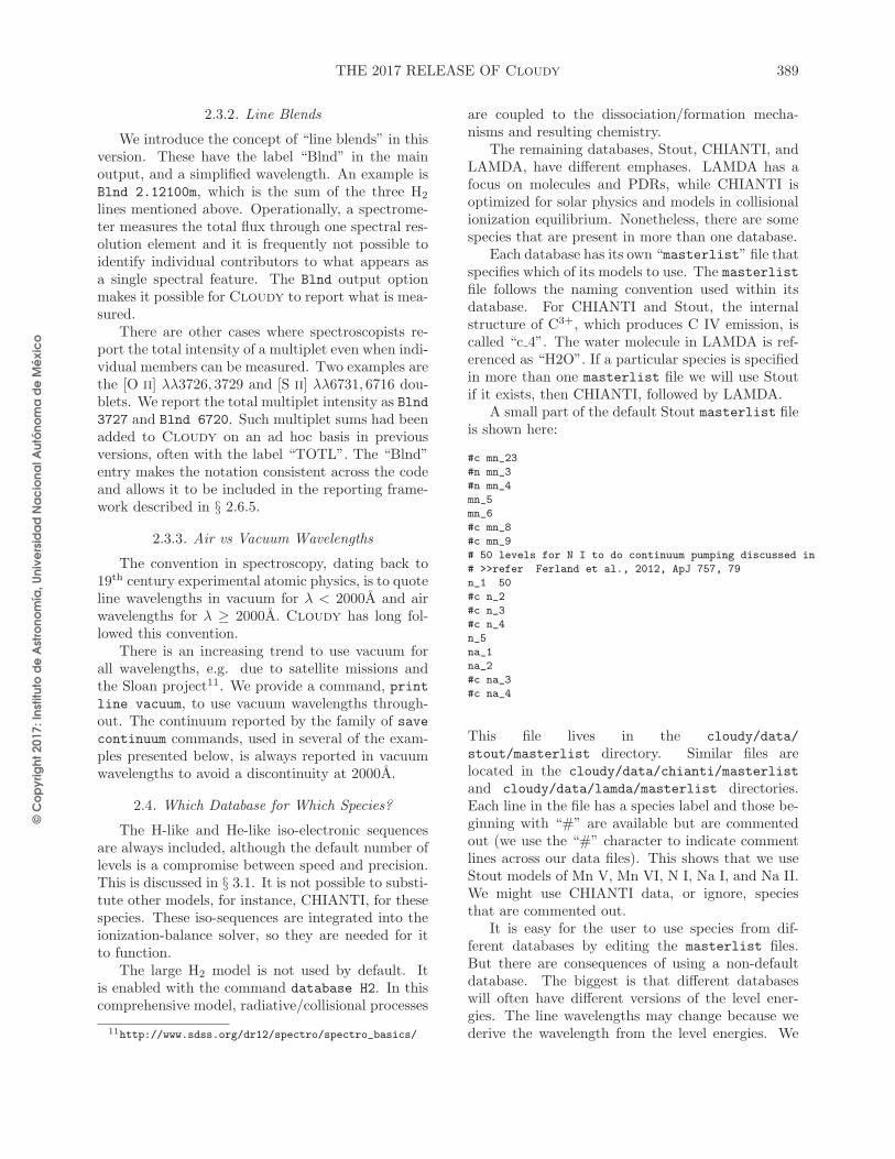
With these databases we predict, by default,more lines in this version of Cloudy than withC13. This actually takes less computer time be-cause of memory and other optimizations describedbelow. Figure 1 compares the density of lines per1000 km s−1 velocity interval for C13, given as theblack dots, and our default setup for C17, the reddots. Most spectral regions now have more lines,often by up to 50%.
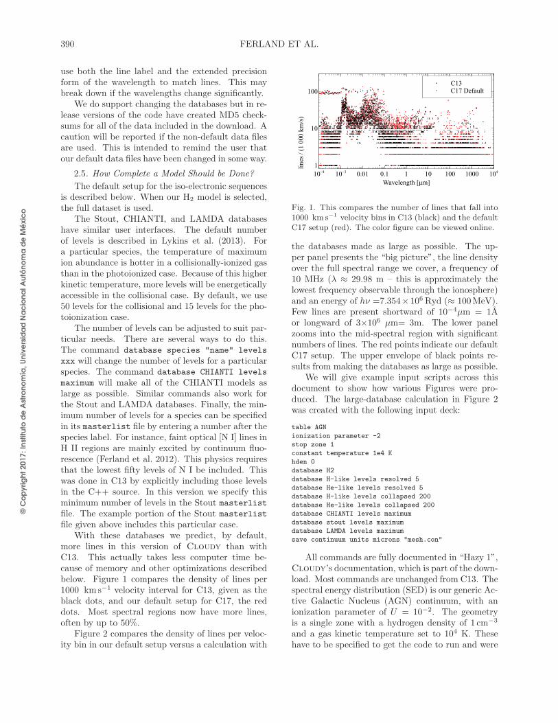
Figure 2 compares the density of lines per veloc-ity bin in our default setup versus a calculation with
Fig. 1. This compares the number of lines that fall into1000 km s−1 velocity bins in C13 (black) and the defaultC17 setup (red). The color figure can be viewed online.
the databases made as large as possible. The up-per panel presents the “big picture”, the line densityover the full spectral range we cover, a frequency of10 MHz (λ ≈ 29.98 m – this is approximately thelowest frequency observable through the ionosphere)and an energy of hν =7.354×10⁶ Ryd (≈ 100MeV).Few lines are present shortward of 10−4µm = 1Aor longward of 3×106 µm= 3m. The lower panelzooms into the mid-spectral region with significantnumbers of lines. The red points indicate our defaultC17 setup. The upper envelope of black points re-sults from making the databases as large as possible.
We will give example input scripts across thisdocument to show how various Figures were pro-duced. The large-database calculation in Figure 2was created with the following input deck:
table AGN
ionization parameter -2
stop zone 1
constant temperature 1e4 K
hden 0
database H2
database H-like levels resolved 5
database He-like levels resolved 5
database H-like levels collapsed 200
database He-like levels collapsed 200
database CHIANTI levels maximum
database stout levels maximum
database LAMDA levels maximum
save continuum units microns "mesh.con"
All commands are fully documented in “Hazy 1”,Cloudy’s documentation, which is part of the down-load. Most commands are unchanged from C13. Thespectral energy distribution (SED) is our generic Ac-tive Galactic Nucleus (AGN) continuum, with anionization parameter of U = 10−2. The geometryis a single zone with a hydrogen density of 1 cm−3
and a gas kinetic temperature set to 104 K. Thesehave to be specified to get the code to run and were

© C
op
yri
gh
t 2
01
7: In
stitu
to d
e A
stro
no
mía
, U
niv
ers
ida
d N
ac
ion
al A
utó
no
ma
de
Mé
xic
o
THE 2017 RELEASE OF Cloudy 391
Fig. 2. This shows the number of lines that fall into1000 km/s velocity bins, across the spectrum. The redpoints for default setup and the black points give thenumber of lines the are predicted when the databasesare made as large as possible. The upper panel showsthe full spectral range considered by the code, while thelower panel shows the peak of the line density. The colorfigure can be viewed online.
chosen to do the simplest and fastest calculation. Asdescribed here, the database commands are new inC17 and control the behavior of the databases.
The number of lines per spectral bin is one of theitems in the file produced by the save continuum
command. The width of each continuum bin, or,equivalently, the spectral resolution, can be ad-justed in two ways. The default continuum meshcan be changed by a uniform scale factor with theset continuum resolution ... command. Thismethod is used in several simulations presented be-low to increase the spectral resolution to highlightparticular issues in the spectrum. Alternatively, theinitialization file continuum mesh.ini in the data
directory can be changed to alter the default contin-uum mesh. This second method was used to makethe C13 and C17 continuum meshes the same, toallow the comparison in Figure 1.
Figure 2 shows that it is possible to predict avery large number of lines, but this comes at greatcost. The default C17 calculation took 4.3 s on anIntel Core I7 processor while the calculation usingthe large databases took 1822 s, roughly half an hour.It would not now be feasible to use the full databasesin a realistic calculation in which the temperature
solver is used and the cloud has a significant columndensity so that optical depths are important.
2.6. Generating Reports
2.6.1. database print
The command database print generates a re-port listing all species. The following would generatea report for Cloudy in its default setup:
test
database print
This command was used to generate Tables 2 and 3giving the default setup for the one- and two-electroniso-sequences. A small portion of the report for theStout, CHIANTI, and LAMDA databases follows:
Using LAMDA model SO with 70 levels of 91 available.
Using LAMDA model SiC2 with 40 levels of 40 available.
Using LAMDA model CS with 31 levels of 31 available.
Using LAMDA model C2H with 70 levels of 102 available.
Using LAMDA model OH+ with 49 levels of 49 available.
Using STOUT spectrum Al 1 (species: Al) with 15 levels of 187 available.
Using STOUT spectrum Al 3 (species: Al+2) with 15 levels of 83 available.
Using STOUT spectrum Al 4 (species: Al+3) with 15 levels of 115 available.
Using STOUT spectrum Zn 2 (species: Zn+) with 15 levels of 27 available.
Using STOUT spectrum Zn 4 (species: Zn+3) with 2 levels of 2 available.
Using CHIANTI spectrum Al 2 (species: Al+) with 15 experimental energy levels of 20
available.
Using CHIANTI spectrum Al 5 (species: Al+4) with 3 experimental energy levels of 3
available.
Using CHIANTI spectrum Al 7 (species: Al+6) with 15 experimental energy levels of 15
available.
Using CHIANTI spectrum Al 8 (species: Al+7) with 15 experimental energy levels of 20
available.
Using CHIANTI spectrum Al 9 (species: Al+8) with 15 experimental energy levels of 54
available.
Each line of output gives the database name, thespectroscopic designation, the species designation,the number of levels used, and the total numberavailable. With CHIANTI there is the further op-tion to use all levels, or only those with experimental(measured) energies.
2.6.2. save species labels all
The save species labels all command willproduce a file containing the full list of species labels.One can generate this list by running the followinginput deck:
test
save species labels "test.slab" all
Table 1 shows a small part of the resulting output.There are several important points in this Table.First, several species do not list a database. Thecases of “H+”, “He+2”, and “C+6” are bare nucleiand have no electronic levels, while the negative hy-drogen ion“H-” and the molecules “HeH+”, “C2+”and “CN+” do have internal levels in nature, butwe currently do not have models of these systems.The remainder are treated with one of the databasesdescribed above. Although many of these specieshave no internal structure, other species properties,
© C
op
yri
gh
t 2
01
7: In
stitu
to d
e A
stro
no
mía
, U
niv
ers
ida
d N
ac
ion
al A
utó
no
ma
de
Mé
xic
o
392 FERLAND ET AL.
TABLE 1
SAVE SPECIES LABEL EXAMPLE
Species label Database
H H-like
H+
H-
He He-like
He+ H-like
He+2
HeH+
C Stout
C+ Stout
C+2 Stout
C+3 CHIANTI
C+4 He-like
C+5 H-like
C+6
C2+
C2H LAMDA
NH3 LAMDA
CN LAMDA
CN+
HCN LAMDA
especially the column density, are computed and re-ported.
Note a likely source of confusion. As describedabove, “C+2” is doubly ionized carbon, while “C2+”is an ion of molecular carbon.
2.6.3. print citation
The print citation command reports the ADSlinks to papers defining the databases we use. Weencourage users to cite the original source of any datathat played an important role in an investigation.This will support and encourage atomic, molecular,and chemical physicists to continue their valuablework.
2.6.4. save species Commands
It is easy to report internal properties of a species,such as the column density or population of a par-ticular level. The following is an example of a save
species command used to report the column densi-ties of several species and the visual extinction:
save species column densities "test.col"
"e-"
"CO[2]"
"C[1:5]"
"H2"
"H"
"H+"
"*AV"
end of species
The total column density of electrons, H2, H0, and
H+ would be reported, along with the population inthe J = 1 level of CO, and the first five levels of C0.Note that the level index within the “[xx:yy]” countsfrom a lowest level of 1.
2.6.5. Save line labels
The save line labels command creates a filelisting all spectral-line labels and wavelengths in thesame format as they appear in the main output’semission-line list. This is a useful way to obtain a listof lines to use when looking for a specific line. Thefile is tab-delimited, with the first column giving theline’s index within the large stack of spectral lines,the second giving the character string that identifiesthe line in the output, and the third giving the line’swavelength in any of several units. Each entry endswith a description of the spectral line. Lines derivedfrom databases (CHIANTI, Stout, LAMDA) are fol-lowed by a comment that contains the database oforigin and the indices of the energy levels, as listedin the original data.
An example of some of its output follows:
4 Inci 0 total luminosity in incident continuum
5 TotH 0 total heating, all forms, information since individuals
added later
6 TotC 0 total cooling, all forms, information since individuals
added later
1259 H 1 911.759A radiative recombination continuum
1260 H 1 3646.00A radiative recombination continuum
1261 H 1 3646.00A radiative recombination continuum
1262 H 1 8203.58A radiative recombination continuum
3552 H 1 1215.68A H-like, 1 3, 1^2S - 2^2P
3557 H 1 1025.73A H-like, 1 5, 1^2S - 3^2P
3562 H 1 972.543A H-like, 1 8, 1^2S - 4^2P
5328 Ca B 1640.00A case a or case b from Hummer & Storey tables
5329 Ca B 1215.23A case a or case b from Hummer & Storey tables
73487 CO 2600.05m LAMDA, 1 2
73492 CO 1300.05m LAMDA, 2 3
73497 CO 866.727m LAMDA, 3 4
85082 C 3 1908.73A Stout, 1 3
85087 C 3 1906.68A Stout, 1 4
85092 C 3 977.020A Stout, 1 5
180217 Al 8 5.82933m CHIANTI, 1 2
180222 Al 8 2139.33A CHIANTI, 1 4
180227 Al 8 381.132A CHIANTI, 1 8
312763 H2 1.13242m diatoms lines
312768 H2 1.26316m diatoms lines
312854 Blnd 2798.00A Blend: "Mg 2 2795.53A"+"Mg 2 2802.71A"
312855 Blnd 615.000A Blend: "Mg10 609.794A"+"Mg10 624.943A"
3. THE IONIZATION EQUILIBRIUM
Our goal is to compute the ionization for a verywide range of densities and temperatures, as shownin Figures 17 and 18 of C13, for the first thirty el-ements and all of their ions.12 This developmentis complete for the H- and He-like iso-electronic se-quences, but is still in progress for many-electron sys-tems. This is challenging because of limitations in
12Those figures were created using the output of
grid extreme from our test suite.
© C
op
yri
gh
t 2
01
7: In
stitu
to d
e A
stro
no
mía
, U
niv
ers
ida
d N
ac
ion
al A
utó
no
ma
de
Mé
xic
o
THE 2017 RELEASE OF Cloudy 393
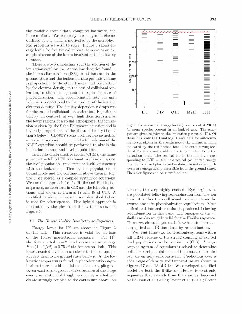
the available atomic data, computer hardware, andhuman effort. We currently use a hybrid scheme,outlined below, which is motivated by the astrophys-ical problems we wish to solve. Figure 3 shows en-ergy levels for five typical species, to serve as an ex-ample of some of the issues involved in the followingdiscussion.
There are two simple limits for the solution of theionization equilibrium. At the low densities found inthe interstellar medium (ISM), most ions are in theground state and the ionization rate per unit volumeis proportional to the atom density multiplied eitherby the electron density, in the case of collisional ion-ization, or the ionizing photon flux, in the case ofphotoionization. The recombination rate per unitvolume is proportional to the product of the ion andelectron density. The density dependence drops outfor the case of collisional ionization (see Equation 4below). In contrast, at very high densities, such asthe lower regions of a stellar atmosphere, the ioniza-tion is given by the Saha-Boltzmann equation and isinversely proportional to the electron density (Equa-tion 5 below). Cloudy spans both regions so neitherapproximation can be made and a full solution of theNLTE equations should be performed to obtain theionization balance and level populations.
In a collisional-radiative model (CRM), the namegiven to the full NLTE treatment in plasma physics,the level populations are determined self-consistentlywith the ionization. That is, the populations inbound levels and the continuum above them in Fig-ure 3 are solved as a coupled system of equations.We use this approach for the H-like and He-like iso-sequences, as described in C13 and the following sec-tions, and shown in Figures 17 and 18 of C13. Amodified two-level approximation, described below,is used for other species. This hybrid approach ismotivated by the physics of the systems shown inFigure 3.
3.1. The H- and He-like Iso-electronic Sequences
Energy levels for H0 are shown in Figure 3on the left. This structure is valid for all ionsof the H-like isoelectronic sequence. For H0,the first excited n = 2 level occurs at an energyE ≈ (1− 1/n2) ≈ 0.75 of the ionization limit. Thislowest excited level is much closer to the continuumabove it than to the ground state below it. At the lowkinetic temperatures found in photoionization equi-librium there should be little collisional coupling be-tween excited and ground states because of this largeenergy separation, although very highly excited lev-els are strongly coupled to the continuum above. As
Fig. 3. Experimental energy levels (Kramida et al. 2014)for some species present in an ionized gas. The ener-gies are given relative to the ionization potential (IP). Ofthese ions, only O III and Mg II have data for autoioniz-ing levels, shown as the levels above the ionization limitindicated by the red hashed box. The autoionizing lev-els of Mg II are not visible since they are far above theionization limit. The vertical bar in the middle, corre-sponding to E/IP = 0.05, is a typical gas kinetic energyin a photoionized plasma and is shown to indicate whichlevels are energetically accessible from the ground state.The color figure can be viewed online.
a result, the very highly excited “Rydberg” levelsare populated following recombination from the ionabove it, rather than collisional excitation from theground state, in photoionization equilibrium. Mostoptical and infrared emission is produced followingrecombination in this case. The energies of the n-shells are also roughly valid for the He-like sequence.These two-electron systems behave in a similar man-ner; optical and IR lines form by recombination.
We treat these two iso-electronic systems with afull CRM because of the strong coupling of excitedlevel populations to the continuum (C13). A largecoupled system of equations is solved to determineboth the level populations and the ionization, so thetwo are entirely self-consistent. Predictions over awide range of density and temperature are shown inFigures 17 and 18 of C13. We developed a unifiedmodel for both the H-like and He-like isoelectronicsequences that extends from H to Zn, as describedby Bauman et al. (2005); Porter et al. (2007); Porter
© C
op
yri
gh
t 2
01
7: In
stitu
to d
e A
stro
no
mía
, U
niv
ers
ida
d N
ac
ion
al A
utó
no
ma
de
Mé
xic
o
394 FERLAND ET AL.
& Ferland (2007); Porter et al. (2012) and Luridia-na et al. (2009), As shown in C13, and previouslyby Ferland & Rees (1988), our model of the ioniza-tion and chemistry of hydrogen does go to the cor-rect limits at high (LTE) and low (ISM) densities,and to the strict thermodynamic equilibrium (STE)limit when exposed to a true blackbody. This is onlypossible when the ionization and level populationsare self-consistently determined by solving the fullcollisional-radiative problem.
3.1.1. Recent Developments
The H- and He-like isoelectronic-sequences, cou-pled with the cosmic abundances of the elements,cause their spectra to fall into two very differentregimes. For brevity, we refer to these as iso-sequences in the following. Hydrogen and heliumhave low nuclear charge Z and so have low ioniza-tion potentials, IP ∼ Z2. As a result, H i, He i,and He ii emission is produced in gas with nebulartemperatures, ≈ 104 K, and occurs mainly in the op-tical and infrared. A goal of the current developmentis the prediction of highly accurate line emissivitiesas a step towards measuring the primordial heliumabundance (Porter et al. 2007).
The next most abundant elements, starting withcarbon (Z = 6), have high ionization potentials,IP ≥ 62 Ryd, so are produced in very hot gas,T ≥ 106 K, and emit X-rays (Porter & Ferland2007; Porter et al. 2006). Heavy elements of theseiso-sequences fall into very different spectral regimesthan hydrogen and helium, probe gas with very dif-ferent physical conditions, and so are found in dis-tinctly different environments.
The high precision needed for primordial heliummeasurements means that the atomic data must bequite accurate. We are revisiting this problem. Theoriginal papers on H i and He i emission (Brockle-hurst 1971, 1972; Benjamin et al. 1999; Hummer &Storey 1987) all used the Pengelly & Seaton (1964)theory of l-changing collisions. Vrinceanu & Flan-nery (2001b,a) and Vrinceanu et al. (2012) presentan improved theory for these collisions, which pre-dict rate coefficients that are ≈6 times smaller. Wehave used these newer rates in most of our publishedwork (Bauman et al. 2005; Porter et al. 2007; Porter& Ferland 2007; Porter et al. 2012; Luridiana et al.2009), and in C13.
There are good reasons, outlined in Guzmanet al. (2016), to prefer the Pengelly & Seaton (1964)theory. Guzman et al. (2017b) extend this treatmentto He-like systems, in which the low-l S, P, and Dstates are not energy-degenerate, so an extra cut-off
energy term is applied to the probability integral asin Pengelly & Seaton (1964). Guzman et al. (2017b)also improve the Pengelly & Seaton (1964) approx-imations to deal with low densities and high tem-peratures, where the original formulae could producenegative values. They call this the modified Pengelly& Seaton (1964, PS-M) approach. Williams et al.(2017) extend the semi-classical theory of Vrinceanu& Flannery (2001b) to provide thermodynamicallyconsistent l-changing rates, which are found to agreequite closely with the results of the other approaches.
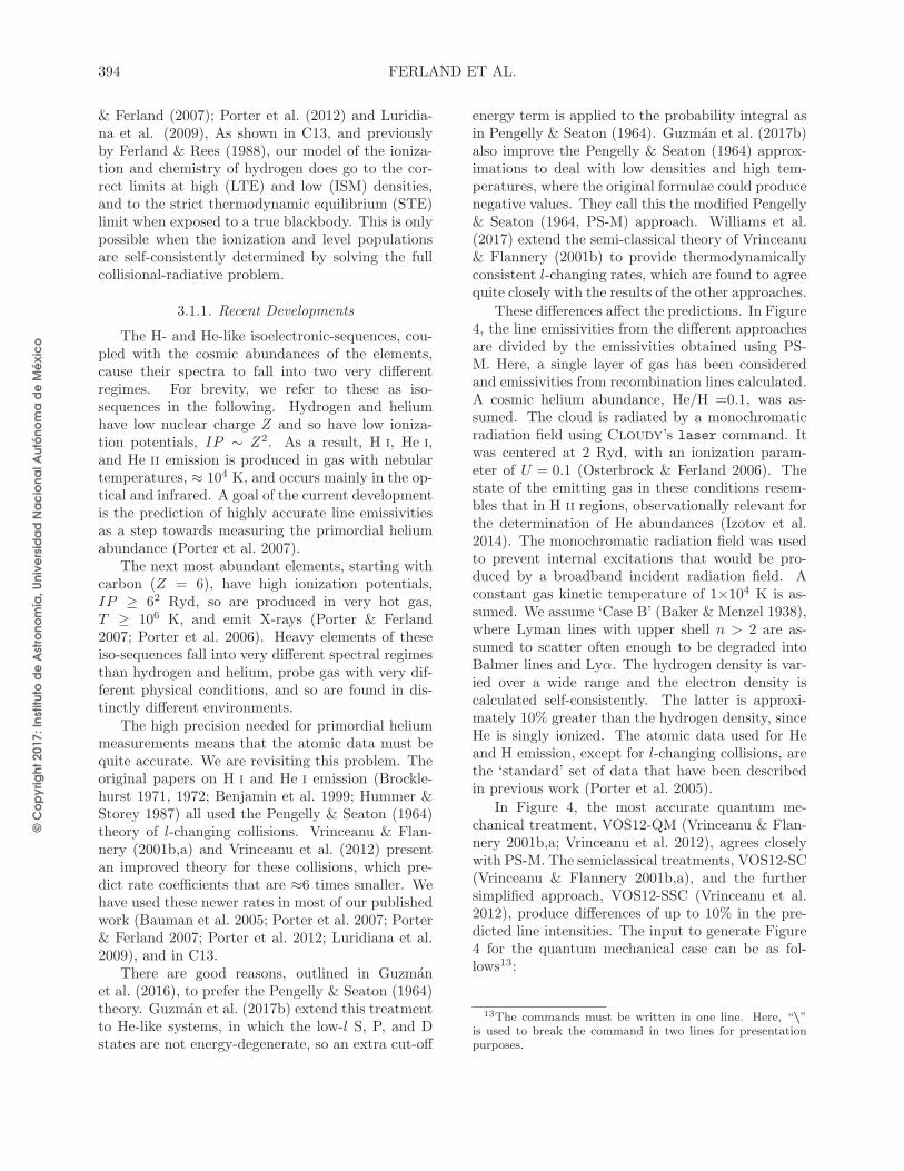
These differences affect the predictions. In Figure4, the line emissivities from the different approachesare divided by the emissivities obtained using PS-M. Here, a single layer of gas has been consideredand emissivities from recombination lines calculated.A cosmic helium abundance, He/H =0.1, was as-sumed. The cloud is radiated by a monochromaticradiation field using Cloudy’s laser command. Itwas centered at 2 Ryd, with an ionization param-eter of U = 0.1 (Osterbrock & Ferland 2006). Thestate of the emitting gas in these conditions resem-bles that in H ii regions, observationally relevant forthe determination of He abundances (Izotov et al.2014). The monochromatic radiation field was usedto prevent internal excitations that would be pro-duced by a broadband incident radiation field. Aconstant gas kinetic temperature of 1×10⁴ K is as-sumed. We assume ‘Case B’ (Baker & Menzel 1938),where Lyman lines with upper shell n > 2 are as-sumed to scatter often enough to be degraded intoBalmer lines and Lyα. The hydrogen density is var-ied over a wide range and the electron density iscalculated self-consistently. The latter is approxi-mately 10% greater than the hydrogen density, sinceHe is singly ionized. The atomic data used for Heand H emission, except for l-changing collisions, arethe ‘standard’ set of data that have been describedin previous work (Porter et al. 2005).
In Figure 4, the most accurate quantum me-chanical treatment, VOS12-QM (Vrinceanu & Flan-nery 2001b,a; Vrinceanu et al. 2012), agrees closelywith PS-M. The semiclassical treatments, VOS12-SC(Vrinceanu & Flannery 2001b,a), and the furthersimplified approach, VOS12-SSC (Vrinceanu et al.2012), produce differences of up to 10% in the pre-dicted line intensities. The input to generate Figure4 for the quantum mechanical case can be as fol-lows13:
13The commands must be written in one line. Here, “\”is used to break the command in two lines for presentation
purposes.

© C
op
yri
gh
t 2
01
7: In
stitu
to d
e A
stro
no
mía
, U
niv
ers
ida
d N
ac
ion
al A
utó
no
ma
de
Mé
xic
o
THE 2017 RELEASE OF Cloudy 395
laser 2
ionization parameter -1
hden 4
element helium abundance -1
init file "hheonly.ini"
stop zone 1
set dr 0
database he-like resolved levels 30
database he-like collapsed levels 170
database he-like collisions l-mixing S62 \
no degeneracy thermal VOS12 quantal
constant temperature 4
case b no photoionzation no Pdest
no scattering escape
no induced processes
iterate
normalise to "He 1" 4471.49A
monitor line luminosity "He 1" 7281.35A \
-18.8686
In this input, the no photoionization option isadded to case b to suppress photoionization fromexcited levels. Then, the pumping of the levels by theresulting photon field is removed by turning off thedestruction of Lyman lines with the no Pdest op-tion. The density is set to 104 cm−3 using the hden 4
command, and the temperature is kept constant withconstant temperature 4. The commands:
stop zone 1
set dr 0
define a layer of gas of 1 cm thickness. The com-mands:
no scattering escape
no induced processes
prevent losses due to scattering, so that all Ly-man lines are degraded into Balmer lines. Themonitor line luminosity ... command com-pares the computed luminosities ( erg s−1) of selectedHe i lines against the reference values given by thePS method. Luminosities can be directly translatedinto emissivities as the thickness of the gas is 1 cm.
Figure 4 has been computed extending tothe n = 200 shell using the database he-like
resolved/collapsed levels commands describedin § 3.1.2. Most of the higher n-shells are col-lapsed (C13, Figure 1) assuming a statistical pop-ulation for the l-subshells, while the low-n levelsare resolved. The number of resolved levels neededis determined by the critical density for l-mixing,where collisional transition rates exceed radiative de-cay rates, as shown in figure 4 of Pengelly & Seaton
(1964). The number of resolved n-shells used to pre-dict the lines in Figure 4 has been varied from n = 60at the lowest density to n = 20 at the highest density.
Commands are provided to select the preferredl-changing theory in the input file for Cloudy. Thecommand to use PS-M is:
database he-like collisions l-mixing S62 \
no degeneracy Pengelly
The keyword S62 in this command tells Cloudy
to use the Seaton (1962) electron impact cross sec-tions for the l-changing collisions of the highly non-degenerate l < 3 subshells (see Guzman et al. 2017b).The keyword no degeneracy uses an energy crite-rion (Pengelly & Seaton 1964) to account for thenon-degeneracy of the l-subshells of He i Rydberglevels (see above). Calculations using the originalformulas provided by Pengelly & Seaton (1964) canbe used by adding the keyword Classic.
VOS12-QM rate coefficients can be used with thecommand:
database he-like collisions l-mixing S62 \
no degeneracy thermal VOS12 Quantal
where the keyword thermal tells Cloudy to per-form a Maxwell average for the cross sections. Bydefault, the effective coefficients will not be Maxwellaveraged, and energies of the collision particles willbe taken to be kT . The evaluation at a single energykT is significantly faster.
The VOS12-QM theory needs a larger numberof operations than the analytic PS-M approach. Italso needs a numerical integration of the collisionprobability to obtain the cross sections. These maybe integrated once more to obtain the Maxwell av-eraged coefficients, making this method computa-tionally slow. Simulations using VOS12-QM cal-culations are ≈ 60 times slower than those usingPS-M. The computational cost of VOS12-QM cal-culations makes PS-M method the preferred one.The VOS12-QM method is recommended when veryhigh-precision results are required.
Finally VOS12-SC and VOS12-SSC can be ob-tained using the commands:
database he-like collisions l-mixing S62 \
thermal Vrinceanu
database he-like collisions l-mixing S62 \
VOS12 semiclassical
respectively. While VOS12-SSC cross-sections canbe obtained with an analytical formula, VOS12-SCneed a double integration making them as computa-tionally slow as VOS12-QM.
© C
op
yri
gh
t 2
01
7: In
stitu
to d
e A
stro
no
mía
, U
niv
ers
ida
d N
ac
ion
al A
utó
no
ma
de
Mé
xic
o
396 FERLAND ET AL.
✵�✁✂
✶
✶�✵✂
✶�✶
■✄■P☎✆✝
❱✞✟✠✡☛✟☞❱✞✟✠✡☛✟✟☞❱✞✟✠✡☛✌✍
✵�✁✂
✶
✶�✵✂
✶�✶
■✄■P☎✆✝
✵�✁✂
✶
✶�✵✂
✶�✶
■✄■P☎✆✝
✵�✁✂
✶
✶�✵✂
✶�✶
■✄■P☎✆✝
✶✵✵✵✵ ✶✎✏✵✂
❧ ✑✒✓
✵�✁✂
✶
✶�✵✂
✶�✶
■✄■P☎✆✝
✶✵✵✵✵ ✶✎✏✵✂
❧ ✑✒✓
♥❍❂✶✵ ✥✔
✲✕♥❍❂✶✵
✷✥✔
✲✕
♥❍❂✶✵
✹✥✔
✲✕♥❍❂✶✵
✕✥✔
✲✕
♥❍❂✶✵
✺✥✔
✲✕♥❍❂✶✵
✻✥✔
✲✕
♥❍❂✶✵
✽✥✔
✲✕♥❍❂✶✵
✼✥✔
✲✕
♥❍❂✶✵
✾✥✔
✲✕♥❍❂✶✵
✖✗✥✔
✲✕
Fig. 4. Ratios of He I lines using the different datasetswith respect to PS-M, see text for details. Figure from(Guzman et al. 2017b). The color figure can be viewedonline.
It is not now possible to experimentally deter-mine which of the theories mentioned above is morecorrect, although we prefer the PS-M approach.Guzman et al. (2017a) outline an astronomical ob-servation that, while difficult, could conclusively de-termine which l-changing theory holds.
3.1.2. Adjusting the Size of the Model
Our models of the H- and He- like iso-sequenceshave a mixture of resolved and collapsed levels, asshown in Figure 1 of C13. Resolved levels are rela-tively expensive to compute due to the need to eval-uate the l-changing collision rates described above.Collapsed levels assume that the l-levels are popu-lated according to their statistical weight within then shell, so this expense is avoided.
The number of resolved and collapsed levels arecontrolled by a family of commands similar to
database H-like hydrogen levels resolved 10
database H-like hydrogen levels collapsed 30
database H-like helium levels resolved 10
database H-like helium levels collapsed 30
database He-like helium levels resolved 10
database He-like helium levels collapsed 30
This example resolves n ≤ 10 for H i, He i, andHe ii and adds 30 collapsed levels to make each atomextend through n = 40. These commands work forH-like and He-like ions of all elements up throughzinc (Z=30).
The command:
database print
generates a report summarizing all databases in useduring the current calculation. This includes thenumber of resolved and collapsed levels for the iso-sequences. By default we resolve n ≤ 10 with anadditional 15 collapsed levels for H i and He ii, andn ≤ 6 as resolved with an additional 20 collapsedlevels for He i.
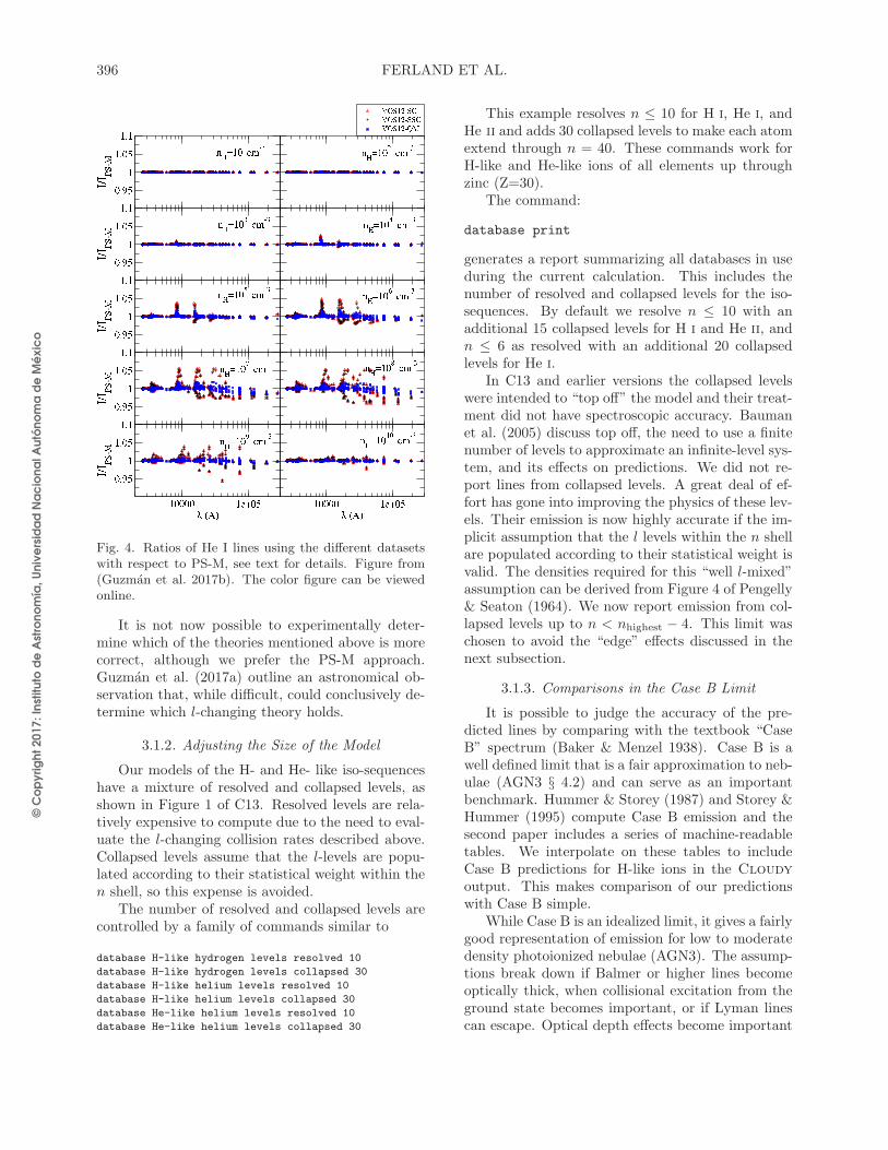
In C13 and earlier versions the collapsed levelswere intended to “top off” the model and their treat-ment did not have spectroscopic accuracy. Baumanet al. (2005) discuss top off, the need to use a finitenumber of levels to approximate an infinite-level sys-tem, and its effects on predictions. We did not re-port lines from collapsed levels. A great deal of ef-fort has gone into improving the physics of these lev-els. Their emission is now highly accurate if the im-plicit assumption that the l levels within the n shellare populated according to their statistical weight isvalid. The densities required for this “well l-mixed”assumption can be derived from Figure 4 of Pengelly& Seaton (1964). We now report emission from col-lapsed levels up to n < nhighest − 4. This limit waschosen to avoid the “edge” effects discussed in thenext subsection.
3.1.3. Comparisons in the Case B Limit
It is possible to judge the accuracy of the pre-dicted lines by comparing with the textbook “CaseB” spectrum (Baker & Menzel 1938). Case B is awell defined limit that is a fair approximation to neb-ulae (AGN3 § 4.2) and can serve as an importantbenchmark. Hummer & Storey (1987) and Storey &Hummer (1995) compute Case B emission and thesecond paper includes a series of machine-readabletables. We interpolate on these tables to includeCase B predictions for H-like ions in the Cloudy
output. This makes comparison of our predictionswith Case B simple.
While Case B is an idealized limit, it gives a fairlygood representation of emission for low to moderatedensity photoionized nebulae (AGN3). The assump-tions break down if Balmer or higher lines becomeoptically thick, when collisional excitation from theground state becomes important, or if Lyman linescan escape. Optical depth effects become important

© C
op
yri
gh
t 2
01
7: In
stitu
to d
e A
stro
no
mía
, U
niv
ers
ida
d N
ac
ion
al A
utó
no
ma
de
Mé
xic
o
THE 2017 RELEASE OF Cloudy 397
in high radiation-density environments such as theinner regions of active galactic nuclei. Collisionalcontributions become important when suprathermalelectrons are present as in X-ray ionized neutral gas(Spitzer & Tomasko 1968), or for hot regions such asvery low metallicity nebulae. The Lyman lines maynot be optically thick in low column density clouds.These processes are treated self-consistently in anycomplete Cloudy calculation.
Larger models, with more levels, make the spec-trum more accurate, at the cost of longer executiontimes and higher memory requirements. The defaultH i model is a compromise between performance andaccuracy.
Figure 5 compares our predictions with Storey &Hummer (1995) for a typical “nebular” temperature,Te = 104 K, and two densities, n(H) = 104 cm−3 and107 cm−3. The lower two panels show predictions ofour default model at the two densities while the up-per panel shows predictions at the lower density witha greatly increased number of resolved and collapsedlevels.
In a normal calculation, Cloudy determines theline optical depths self-consistently, assuming thecomputed column densities, level populations, andline broadening. A Case B command exists to createthese conditions and to make these comparisons pos-sible while computing a single “zone”, a thin layer ofgas. The command sets the Lyman line optical depthto a large number and suppresses collisional excita-tion out of n = 2, to be consistent with the Storey& Hummer (1995) implementation of Case B. Thiscommand was included in the input script used toto create Figure 5. In previous versions of Cloudy
we also recommended using the Case B commandin certain simple PDR (photodissociation region, orphoton-dominated region) calculations to block Ly-man line fluorescence. As described in § 5.4 below,we now recommend using a different command inthe PDR case, reserving the Case B command forthis purpose only.
The large model reproduces the Storey & Hum-mer (1995) results to high precision. There are dif-ferences at the ∼ 2% level, which we believe to becaused by recent improvements in the collision andrecombination data. This will be the subject of afuture paper (Guzman et al. in preparation).
The middle and lower panels show the results ofapplying our default H imodel (n ≤ 10 resolved withan additional 15 collapsed) to the same density, andto a higher density case. The default model waschosen to reproduce the intensities of the brighter H i
lines to good precision. The large red filled circles
Fig. 5. This shows ratios of our predicted H i emission tothe Storey & Hummer (1995) Case B tables. Calculationsare for Te = 104 K and the indicated densities. The up-per panel, our test case limit caseb h den4 temp4.in.,shows that we reproduce their results to high accuracywhen a large model is used. The default model, chosenas a compromise between speed and accuracy, is shownin the lower two panels. The default model is designed togive higher accuracy for the brighter optical and near-IRlines, plotted as the larger filled circles. Note that eachpanel has a different vertical scale. The color figure canbe viewed online.
in the middle panel indicate lines with intensitiesgreater than 5% that of Hβ. These have deviationsof ∼< 10%.
The eye picks up a trend for the error ratio tomove away from unity along a spectroscopic (thatis, Balmer, Paschen, etc) series, as the upper level nincreases. This is produced by two effects. The firstis an “edge” effect as the upper level approaches theupper limit of the model. (We do not report linesarising from n ≥ nhighest − 4 for this reason.) Thelevel populations for the very highest levels are inac-curate because of their proximity to the large “gap”that exists between the highest level and the continu-um above. The errors at lower n are due to the factthat the lower collapsed levels, 10 < n ≤ 15, are notactually l-mixed at the lower density of 104 cm−3.The density of 107 cm−3 is high enough to l-mix

© C
op
yri
gh
t 2
01
7: In
stitu
to d
e A
stro
no
mía
, U
niv
ers
ida
d N
ac
ion
al A
utó
no
ma
de
Mé
xic
o
398 FERLAND ET AL.
n = 11 so this model is better behaved. These testsshow that the implementation gives reliable resultswhen the number of levels is made large enough.
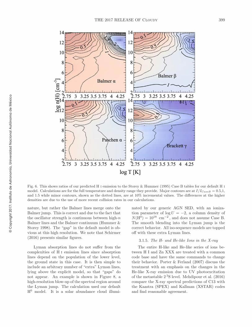
The default model was designed to reproduce theintensities of the brighter H i lines while being com-putationally expeditious. As a test we computed theintensities of four of the most commonly observedH i lines over the density and temperature given inthe Storey & Hummer (1995) tables including theCase B command. The ratio of our predictions totheir Case B values is given in Figure 6. The largestdifferences are at the higher densities where Case Bwould not be expected to apply. These differencesare due to recent improvements in the H0 collisionrates. At the lower densities where Case B mightapply the agreement is good; the default model isgenerally within 10% of Storey & Hummer (1995).
This calculation used our grid command to com-pute the required range of density and temperatureand the save linelist ratio command to savepredictions into a file. The input script is
set save prefix "nt"
case B
hden 4 vary
grid 2 14 .5 log
constant temperature 4 vary
grid 2.7 4.4 0.05 log
#
stop zone 1
set dr 0
laser 2
ionization parameter 0
init "honly.ini"
save grid ".grd"
save linelist ratio ".rat" "nt.lines" last no hash
The save linelist ratio command reads thelist of lines in the file nt.lines and saves them intothe file nt.rat. The list of lines in nt.lines areordered pairs and the ratio of intensities of the firstto second is reported. (The “#” lines are commentsadded to aid the user and are ignored.) The predic-tions in the nt.rat file were combined with the gridmodel parameters saved in the file nt.grd to createthe plot. The nt.lines file contained the followingset of line ratios:
H 1 4340.49A
Ca B 4340.49A
#
H 1 4861.36A
Ca B 4861.36A
#
H 1 6562.85A
Ca B 6562.85A
#
H 1 1.87511m
Ca B 1.87511m
#
H 1 2.16553m
Ca B 2.16553m
Similar tests can be made for other lines of interest.The number of resolved levels must be increased
when higher precision is needed at low densities (Fig-ure 6) or for faint IR / FIR lines (Figure 5). Figure 4of Pengelly & Seaton (1964) can be used as a guide indeciding how many resolved levels are needed. Theirvertical axis is, in effect, the negative log of the hy-drogen density. The lines indicate the critical den-sity, defined in eqn 3.30 of AGN3, where l-changingrates are equal to the radiative decay rate. The l lev-els within the indicated n will be well mixed whenthe density is significantly higher than this criticaldensity. For instance, at a density of 104 cm−3, thefigure shows that the n = 15 shell is at its criti-cal density. Our default model uses collapsed levelsfor 11 ≤ n ≤ 15, causing the residuals in the centerpanel of Figure 5. Our lowest collapsed level, n = 11,has a critical density of ∼ 105.5 cm−3. This is whythe model is so much more accurate, but still notexcellent, at the higher density in the lower panel,107 cm−3.
The user could adjust the model to suit require-ments at a particular density using Case B predic-tions as a guide. We recommend creating a one-zoneCase B simulation with a density and temperatureset to the conditions under study. Then, adjust thesize of the model to achieve the desired accuracy bycomparing the lines of interest with the Storey &Hummer (1995) Case B predictions that are includedin the output.
Making the model large does come at some cost.Tests show that the test suite example pn paris, oneof the original Meudon meeting test cases (Pequignot1986), takes ≈ 27s using the default H0 model on amodern Xeon, while the large model in Figure 5 takes44m 25s.
3.1.4. Convergence of Lines onto RadiativeRecombination Continua
As mentioned above, the finite size of the H0
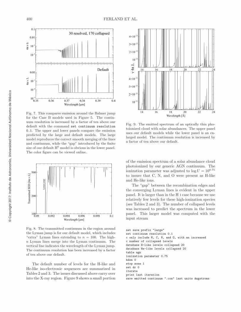
model is one source of deviations from Case B linepredictions in Figure 5. Any finite model will havea “gap” between the highest level and the contin-uum above. This gap is also present in the pre-dicted spectrum, as shown in Figure 7. This showsthe converging high-n Balmer lines and the Balmerjump corresponding to radiative recombination cap-tures to n = 2. The upper panel shows the largemodel used in Figure 5 while the lower is the defaultmodel. There is no “gap” in the large model, or in
© C
op
yri
gh
t 2
01
7: In
stitu
to d
e A
stro
no
mía
, U
niv
ers
ida
d N
ac
ion
al A
utó
no
ma
de
Mé
xic
o
THE 2017 RELEASE OF Cloudy 399
Fig. 6. This shows ratios of our predicted H i emission to the Storey & Hummer (1995) Case B tables for our default H i
model. Calculations are for the full temperature and density range they provide. Major contours are at I/ICaseB = 0.5,1,and 1.5 while minor contours, shown as the dotted lines, are at 10% incremental values. The differences at the higherdensities are due to the use of more recent collision rates in our calculations.
nature, but rather the Balmer lines merge onto theBalmer jump. This is correct and due to the fact thatthe oscillator strength is continuous between high-nBalmer lines and the Balmer continuum (Hummer &Storey 1998). The “gap” in the default model is ob-vious at this high resolution. We note that Schirmer(2016) presents similar figures.
Lyman absorption lines do not suffer from thecomplexities of H i emission lines since absorptionlines depend on the population of the lower level,the ground state in this case. It is then simple toinclude an arbitrary number of “extra” Lyman lines,lying above the explicit model, so that “gaps” donot appear. An example is shown in Figure 8, ahigh-resolution blow-up of the spectral region aroundthe Lyman jump. The calculation used our defaultH0 model. It is a solar abundance cloud illumi-
nated by our generic AGN SED, with an ioniza-tion parameter of logU = −2, a column density ofN(H0) = 1018 cm−2 , and does not assume Case B.The smooth blending into the Lyman jump is thecorrect behavior. All iso-sequence models are toppedoff with these extra Lyman lines.
3.1.5. The H- and He-like Ions in the X-ray
The entire H-like and He-like series of ions be-tween H I and Zn XXX are treated with a commoncode base and have the same commands to changetheir behavior. Porter & Ferland (2007) discuss thetreatment with an emphasis on the changes in theHe-like X-ray emission due to UV photoexcitationof the metastable 2 3S level. Mehdipour et al. (2016)compare the X-ray spectral predictions of C13 withthe Kaastra (SPEX) and Kallman (XSTAR) codesand find reasonable agreement.
© C
op
yri
gh
t 2
01
7: In
stitu
to d
e A
stro
no
mía
, U
niv
ers
ida
d N
ac
ion
al A
utó
no
ma
de
Mé
xic
o
400 FERLAND ET AL.
Fig. 7. This compares emission around the Balmer jumpfor the Case B models used in Figure 5. The contin-uum resolution is increased by a factor of ten above ourdefault with the command set continuum resolution
0.1. The upper and lower panels compare the emissionpredicted by the large and default models. The largemodel reproduces the correct smooth merging of the linesand continuum, while the “gap” introduced by the finitesize of our default H0 model is obvious in the lower panel.The color figure can be viewed online.
Fig. 8. The transmitted continuum in the region aroundthe Lyman jump is for our default model, which includes“extra” Lyman lines extending to n = 100. The high-n Lyman lines merge into the Lyman continuum. Thevertical line indicates the wavelength of the Lyman jump.The continuum resolution has been increased by a factorof ten above our default.
The default number of levels for the H-like andHe-like iso-electronic sequences are summarized inTables 2 and 3. The issues discussed above carry overinto the X-ray region. Figure 9 shows a small portion
Fig. 9. The emitted spectrum of an optically thin pho-toionized cloud with solar abundances. The upper paneluses our default models while the lower panel is an en-larged model. The continuum resolution is increased bya factor of ten above our default.
of the emission spectrum of a solar abundance cloudphotoionized by our generic AGN continuum. Theionization parameter was adjusted to logU = 100.75
to insure that C, N, and O were present as H-likeand He-like ions.
The “gap” between the recombination edges andthe converging Lyman lines is evident in the upperpanel. It is larger than in the H i case because we userelatively few levels for these high-ionization species(see Tables 2 and 3). The number of collapsed levelswas increased to predict the spectrum in the lowerpanel. This larger model was computed with theinput stream
set save prefix "large"
set continuum resolution 0.1
c only include H, C, N, and O, with an increased
c number of collapsed levels
database H-like levels collapsed 20
database He-like levels collapsed 20
table agn
ionization parameter 0.75
hden 0
stop zone 1
set dr 0
iterate
print last iteration
save emitted continuum ".con" last units Angstroms

© C
op
yri
gh
t 2
01
7: In
stitu
to d
e A
stro
no
mía
, U
niv
ers
ida
d N
ac
ion
al A
utó
no
ma
de
Mé
xic
o
THE 2017 RELEASE OF Cloudy 401
TABLE 2
DEFAULT NUMBER OF LEVELS FOR THEH-LIKE ISO-ELECTRONIC SEQUENCE
Element n(res) nls(res) n(coll)
H 10 55 15
He 10 55 15
Li 5 15 2
Be 5 15 2
B 5 15 2
C 5 15 5
N 5 15 5
O 5 15 5
F 5 15 2
Ne 5 15 5
Na 5 15 2
Mg 5 15 5
Al 5 15 2
Si 5 15 5
P 5 15 2
S 5 15 5
Cl 5 15 2
Ar 5 15 2
K 5 15 2
Ca 5 15 2
Sc 5 15 2
Ti 5 15 2
V 5 15 2
Cr 5 15 2
Mn 5 15 2
Fe 5 15 5
Co 5 15 2
Ni 5 15 2
Cu 5 15 2
Zn 5 15 5
The extra levels produce enough lines to fill in the“gap” at this resolution. Regions of significantly in-creased emission produced by the additional levelsare also evident in the larger model.
3.2. A Modified Two-level Approximation for OtherIons
3.2.1. The Two-level Approximation
Textbooks on the interstellar medium (ISM), e.g.Spitzer (1978), Tielens (2005), Osterbrock & Ferland(2006), and Draine (2011), write the ionization bal-ance of an ion as the equivalent two-level system:
n(i+ 1)
n(i)=
Γ(i)
α(i+ 1)ne, (1)
TABLE 3
DEFAULT NUMBER OF LEVELS FOR HE-LIKEISO-ELECTRONIC SEQUENCE
Element n(res) nls(res) n(coll)
He 6 43 20
Li 3 13 2
Be 3 13 2
B 3 13 2
C 5 31 5
N 5 31 5
O 5 31 5
F 3 13 2
Ne 5 31 5
Na 3 13 2
Mg 5 31 5
Al 3 13 2
Si 5 31 5
P 3 13 2
S 5 31 5
Cl 3 13 2
Ar 3 13 2
K 3 13 2
Ca 3 13 2
Sc 3 13 2
Ti 3 13 2
V 3 13 2
Cr 3 13 2
Mn 3 13 2
Fe 5 31 5
Co 3 13 2
Ni 3 13 2
Cu 3 13 2
Zn 5 31 5
where n(i+1) and n(i) are the densities of two adja-cent ionization stages, α(i+ 1) is the total recombi-nation rate coefficient of the ion (cm3 s−1) and Γ(i)is the ionization rate (s−1). In photoionization equi-librium
Γ(i) =
∫φνσν dν , (2)
where φν is the flux of ionizing photons [photons s−1
cm−2 Hz−1], σν is the photoionization cross section[cm−2] and the integral is over ionizing energies. Onthe other hand, in collisional ionization equilibrium
Γ(i) = q(i)ne , (3)
where q(i) is the collisional ionization rate coefficient.

© C
op
yri
gh
t 2
01
7: In
stitu
to d
e A
stro
no
mía
, U
niv
ers
ida
d N
ac
ion
al A
utó
no
ma
de
Mé
xic
o
402 FERLAND ET AL.
In its simplest form, the two-level approximationassumes that recombinations to all excited states willeventually decay to the ground state, and that allionizations occur out of the ground state. Only theionization rate from the ground state and the sum ofrecombination coefficients to all excited states needbe considered, a great savings in data needs.
This two-level approach extends over to thechemistry. Most codes use databases similar to theUMIST Database for Astrochemistry (McElroy et al.2013). Reactions between complex molecules aretreated as a single channel without detailed treat-ment of internal structure. In this approximation,rate coefficients do not have a strong density depen-dence and do not depend on the internal level pop-ulations of the molecule. Most of the chemical dataneeded to implement a more complete model simplydo not currently exist.
In some fields, the two-level approximation iscalled the “coronal” approximation when collisionalionization is dominant. The solar corona has lowdensity and is collisionally ionized. The low densitiesinsure that most of the population is in the groundstate and that recombinations to excited states decayto ground. Emission from the solar photosphere istoo soft to affect the ionization. Cloudy has long in-cluded a coronal command which sets a gas kinetictemperature, informs the code that it is acceptablefor no incident radiation field to be specified, and cal-culates the ionization and emission including thermalcollisions and any light or cosmic rays that may alsobe specified.
3.2.2. The Independent Ionization / EmissionApproximation
Together with the two-level approximation, wecan further assume that emissions from low-lying lev-els are not affected by the ionization / recombinationprocess, so that they can be treated as separate prob-lems. As examples, the C IV λ1549, Mg II λ2978,and [O III] λλ 5007, 4959 multiplets are producedby the lowest excited levels of their ions in Figure 3.These levels are much closer to ground than to thecontinuum, so they should be most directly coupledto the ground state. The fact that, at low particleand photon densities, nearly all of the population ofa species is in the ground state, further justifies thisassumption.
This “independent ionization / emission” approx-imation (IIEA) is also suggested from considera-tion of the relevant timescales. Consider the sim-ple model of the Orion Nebula described by Ferlandet al. (2016). The recombination time of a typical
ion is ≈ 7 yr at a density of n ≈ 104 cm−3. Elec-trons tend to be captured into highly excited states,which have lifetimes of about 10−5 s to 10−8 s, sothe electron quickly falls down to the ground state.The electron remains in the ground state for aboutfive hours before another ionizing photon is absorbedand the process starts again.
Line-emission timescales are much faster, withcollisional excitation timescales of ≈ 105 s at adensity of 104 cm−3 and photon emission occurringwithin τ ≈ 10−7 s for a typical permitted transition.Collisional / emission processes within the low-lyinglevels occur on timescales that are τ ≥ 4 dex fasterthan ionization – recombination. As a result, mostcodes first solve for the ionization distribution of anelement, then for the line emission from each ion.They are treated as separate problems.
This is equivalent to the use of photo-emissioncoefficients (PEC), introduced by Summers et al.(2006) and commonly used in fusion plasmas. Theline emissivity for a transition between excited lev-
els i and j can then be expressed as PEC(exc)σ,i→jnσ,
where the excited levels i and j are assumed to bein equilibrium with the ground or metastable state
σ. Here, PEC(exc)σ,i→j = Ai→jF
(exc)iσ is the excitation
photo-emission coefficient for the i → j transition,
where F(exc)iσ accounts for the collisional-radiative ex-
citation to level i from σ.Systems with an especially complex structure,
such as Fe II, are a major exception to the discus-sion so far. Fe II has levels extending, nearly uni-formly, between the ground state and the contin-uum, as shown in the right of Figure 3. The atomicphysics of Fe II is especially complex due to the factthat it has a half-filled d shell, combined with thenear energy degeneracy of the 3d and 4s electrons.Unfortunately Fe II emission is strong in a numberof astrophysically important classes of objects, in-cluding quasars and shocked regions. This is a worstcase, with our treatment discussed by Verner et al.(1999).
The remainder of this section discusses our imple-mentation of a modified two-level approximation formany-electron systems. The following section dis-cusses our treatment of the bound levels and theiremission.
3.2.3. Ionization / Recombination Rates
Our sources for ionization and recombinationdata for many-electron systems are summarized inC13. Ground and inner-shell photoionization crosssections are given by Verner et al. (1996), andsummed recombination rate coefficients are com-

© C
op
yri
gh
t 2
01
7: In
stitu
to d
e A
stro
no
mía
, U
niv
ers
ida
d N
ac
ion
al A
utó
no
ma
de
Mé
xic
o
THE 2017 RELEASE OF Cloudy 403
puted as in Badnell et al. (2003), Badnell (2006),and are listed on Badnell’s web site14.
We have long used collisional ionization rate co-efficients presented by Voronov (1997). Two re-cent studies, Dere (2007) and Kwon & Savin (2014),have presented new rate coefficients for collisionalionization of some ions. These studies are in verygood agreement with Voronov (1997) for tempera-tures around those of the peak abundance of the ion.Unfortunately, the fitting equations used by Dere(2007) and Kwon & Savin (2014) only return pos-itive values for temperatures around the peak abun-dance of the ion in collisional ionization equilibrium.The Voronov (1997) fits are well behaved over thefull temperature range we cover, 2.7 K to 1010 K.
As described by Lykins et al. (2013), we improvedthe Voronov (1997) fits by rescaling by the ratioof the new to Voronov values at temperatures nearthe peak abundance of the ion. This correction wasusually small, well bellow 20%, so has only modestchanges in results.
3.2.4. Collisional Suppression of DielectronicRecombination (DR)
Dielectronic recombination (DR), a processwhere a free electron is captured by exciting a boundelectron, forming an autoionizing state that can de-cay into bound levels, is the dominant recombinationprocess for most many-electron ions. We mainly usedata from Badnell15, which is also the largest collec-tion available for this process.
Energetically, the DR process occurs via levelswith energies within kT of the ionization limit, so,as shown in the center of Fig 3, it will mainly popu-late levels that are close to the ionization limit. Ofthe ions shown in the Figure, only O iii has low-lyingautoionizing levels, the levels above the ionizationlimit. For many ions, experimental data for suchlow-lying autoionizing levels are either completelymissing or incomplete. The summed DR rates listedon the Badnell web site assume that all these pop-ulations eventually decay to the ground state, anapproximation that must fail at high densities, asquantified below.
It has long been known that DR is suppressed bycollisional ionization at moderate to high densities(Sunyaev & Vainshtein 1968; Burgess & Summers1969; Davidson 1975). Nikolic et al. (2013) extendedprevious work to estimate the extent of this suppres-sion for various iso-electronic sequences. Their figure
14see http://amdpp.phys.strath.ac.uk/tamoc/RR/,
http://amdpp.phys.strath.ac.uk/tamoc/DR/15http://amdpp.phys.strath.ac.uk/tamoc/DR
7 shows that the ionization of low stages of iron canchange by nearly 1 dex at densities of ≈ 1010 cm−3
when suppression is included. As stressed in that pa-per, these results are highly approximate, with theuncertainty in the suppression being of order the cor-rection itself. A full solution of the populations of theexcited states must be done to get the right answer(Summers et al. 2006). Such corrections do allowthe two-level approximation to be applied at higherdensities, although with this uncertainty.
Nikolic et al. (2017, in preparation) revisited theproblem and estimated new suppression factors thatoffer an improvement over the 2013 values. We usethose suppression factors in this release of Cloudy.
3.2.5. Limits of the Two-Level Approximation forthe ionization
Over what density range is the two-level approx-imation valid? How does it fail outside this range?Despite the wide application of this approximation,we do not know of a discussion of these questions.
The two-level approximation will fail when highlyexcited states do not decay to the ground, most of-ten due to collisional ionization at high densities.Highly-excited levels are long lived due to smallerspontaneous decay rates; for hydrogenic systems thelifetime scales as τ ∝ n5 (He et al. 1990). At thesame time, the cross section for collisions increasesfor higher levels as n4. So, compared to electronsin low levels, those in highly excited levels decay tolower levels slowly, and a large probability for colli-sional ionization is the result. Further, at high den-sity and temperature the highly-excited levels of allions will have significant populations, related to thewell-known divergence of the partition function instellar atmospheres (Hubeny &Mihalas 2014). Colli-sional ionization from excited states becomes impor-tant, and the use of summed recombination coeffi-cients becomes highly approximate, so both the two-level approximation and “independent ionization /emission” assumptions break down.
We can use our complete CRM solutions for theH- and He-like isoelectronic sequences to show wherethe two-level approximation fails. In Figure 10 weconsider the ionization of hydrogen in a collision-ally ionized gas at the indicated temperature, shownover a very wide range of density. The Figure, basedon one shown in Wang et al. (2014), shows howcollisional-radiative effects, mainly involving highlyexcited levels, cause the hydrogen ionization to gofrom coronal equilibrium at low-densities to localthermodynamic equilibrium (LTE) at high densities.Figure 5 of Summers et al. (2006) shows a somewhat
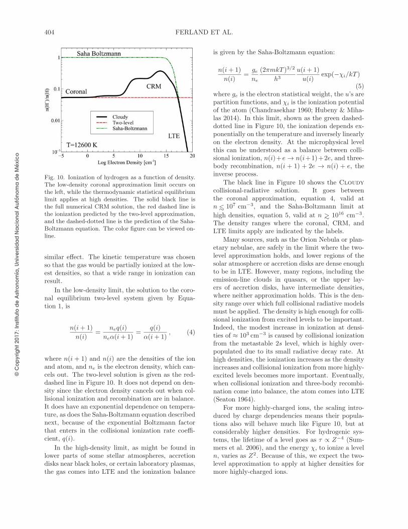
© C
op
yri
gh
t 2
01
7: In
stitu
to d
e A
stro
no
mía
, U
niv
ers
ida
d N
ac
ion
al A
utó
no
ma
de
Mé
xic
o
404 FERLAND ET AL.
Fig. 10. Ionization of hydrogen as a function of density.The low-density coronal approximation limit occurs onthe left, while the thermodynamic statistical equilibriumlimit applies at high densities. The solid black line isthe full numerical CRM solution, the red dashed line isthe ionization predicted by the two-level approximation,and the dashed-dotted line is the prediction of the Saha-Boltzmann equation. The color figure can be viewed on-line.
similar effect. The kinetic temperature was chosenso that the gas would be partially ionized at the low-est densities, so that a wide range in ionization canresult.
In the low-density limit, the solution to the coro-nal equilibrium two-level system given by Equa-tion 1, is
n(i+ 1)
n(i)=
neq(i)
neα(i+ 1)=
q(i)
α(i+ 1), (4)
where n(i + 1) and n(i) are the densities of the ionand atom, and ne is the electron density, which can-cels out. The two-level solution is given as the red-dashed line in Figure 10. It does not depend on den-sity since the electron density cancels out when col-lisional ionization and recombination are in balance.It does have an exponential dependence on tempera-ture, as does the Saha-Boltzmann equation describednext, because of the exponential Boltzmann factorthat enters in the collisional ionization rate coeffi-cient, q(i).
In the high-density limit, as might be found inlower parts of some stellar atmospheres, accretiondisks near black holes, or certain laboratory plasmas,the gas comes into LTE and the ionization balance
is given by the Saha-Boltzmann equation:
n(i+ 1)
n(i)=
gene
(2πmkT )3/2
h3
u(i+ 1)
u(i)exp(−χi/kT )
(5)where ge is the electron statistical weight, the u’s arepartition functions, and χi is the ionization potentialof the atom (Chandrasekhar 1960; Hubeny & Miha-las 2014). In this limit, shown as the green dashed-dotted line in Figure 10, the ionization depends ex-ponentially on the temperature and inversely linearlyon the electron density. At the microphysical levelthis can be understood as a balance between colli-sional ionization, n(i)+e → n(i+1)+2e, and three-body recombination, n(i + 1) + 2e → n(i) + e, theinverse process.
The black line in Figure 10 shows the Cloudy
collisional-radiative solution. It goes betweenthe coronal approximation, equation 4, valid atn ∼< 107 cm−3, and the Saha-Boltzmann limit at
high densities, equation 5, valid at n ∼> 1016 cm−3.The density ranges where the coronal, CRM, andLTE limits apply are indicated by the labels.
Many sources, such as the Orion Nebula or plan-etary nebulae, are safely in the limit where the two-level approximation holds, and lower regions of thesolar atmosphere or accretion disks are dense enoughto be in LTE. However, many regions, including theemission-line clouds in quasars, or the upper lay-ers of accretion disks, have intermediate densities,where neither approximation holds. This is the den-sity range over which full collisional radiative modelsmust be applied. The density is high enough for colli-sional ionization from excited levels to be important.Indeed, the modest increase in ionization at densi-ties of ≈ 103 cm−3 is caused by collisional ionizationfrom the metastable 2s level, which is highly over-populated due to its small radiative decay rate. Athigh densities, the ionization increases as the densityincreases and collisional ionization from more highly-excited levels becomes more important. Eventually,when collisional ionization and three-body recombi-nation come into balance, the atom comes into LTE(Seaton 1964).
For more highly-charged ions, the scaling intro-duced by charge dependencies means their popula-tions also will behave much like Figure 10, but atconsiderably higher densities. For hydrogenic sys-tems, the lifetime of a level goes as τ ∝ Z−4 (Sum-mers et al. 2006), and the energy χ, to ionize a leveln, varies as Z2. Because of this, we expect the two-level approximation to apply at higher densities formore highly-charged ions.
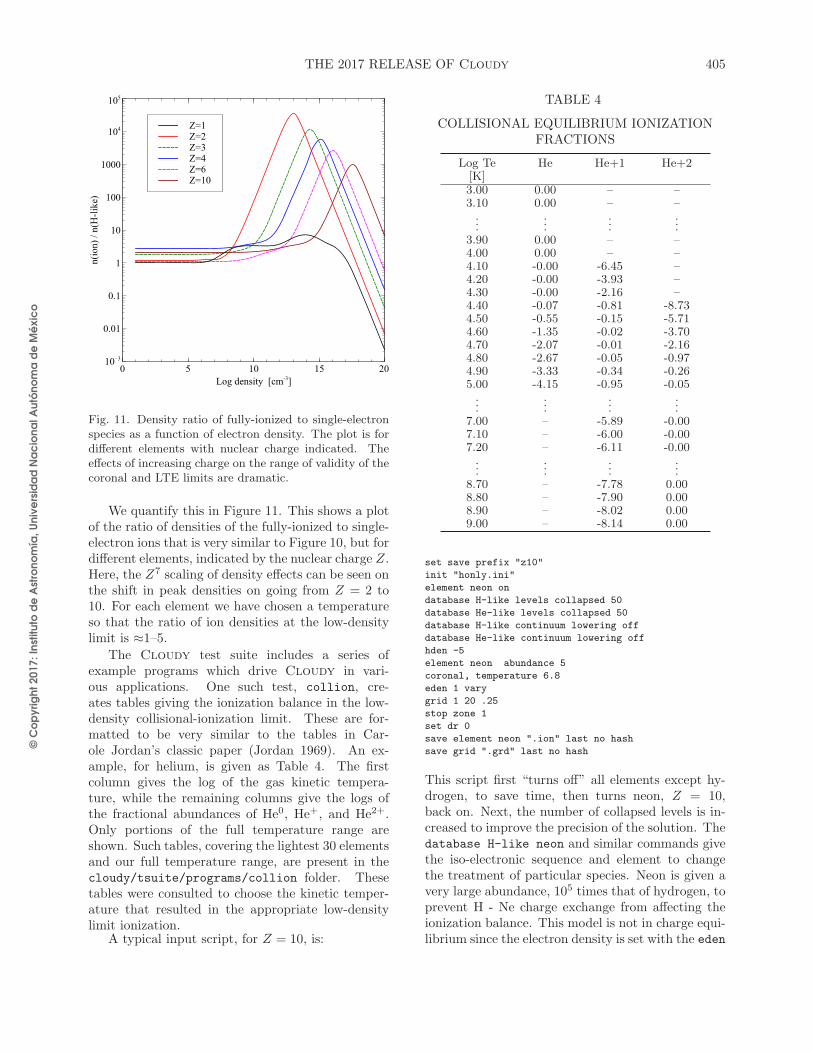
© C
op
yri
gh
t 2
01
7: In
stitu
to d
e A
stro
no
mía
, U
niv
ers
ida
d N
ac
ion
al A
utó
no
ma
de
Mé
xic
o
THE 2017 RELEASE OF Cloudy 405
Fig. 11. Density ratio of fully-ionized to single-electronspecies as a function of electron density. The plot is fordifferent elements with nuclear charge indicated. Theeffects of increasing charge on the range of validity of thecoronal and LTE limits are dramatic.
We quantify this in Figure 11. This shows a plotof the ratio of densities of the fully-ionized to single-electron ions that is very similar to Figure 10, but fordifferent elements, indicated by the nuclear charge Z.Here, the Z7 scaling of density effects can be seen onthe shift in peak densities on going from Z = 2 to10. For each element we have chosen a temperatureso that the ratio of ion densities at the low-densitylimit is ≈1–5.
The Cloudy test suite includes a series ofexample programs which drive Cloudy in vari-ous applications. One such test, collion, cre-ates tables giving the ionization balance in the low-density collisional-ionization limit. These are for-matted to be very similar to the tables in Car-ole Jordan’s classic paper (Jordan 1969). An ex-ample, for helium, is given as Table 4. The firstcolumn gives the log of the gas kinetic tempera-ture, while the remaining columns give the logs ofthe fractional abundances of He0, He+, and He2+.Only portions of the full temperature range areshown. Such tables, covering the lightest 30 elementsand our full temperature range, are present in thecloudy/tsuite/programs/collion folder. Thesetables were consulted to choose the kinetic temper-ature that resulted in the appropriate low-densitylimit ionization.
A typical input script, for Z = 10, is:
TABLE 4
COLLISIONAL EQUILIBRIUM IONIZATIONFRACTIONS
Log Te He He+1 He+2[K]3.00 0.00 – –3.10 0.00 – –...
......
...3.90 0.00 – –4.00 0.00 – –4.10 -0.00 -6.45 –4.20 -0.00 -3.93 –4.30 -0.00 -2.16 –4.40 -0.07 -0.81 -8.734.50 -0.55 -0.15 -5.714.60 -1.35 -0.02 -3.704.70 -2.07 -0.01 -2.164.80 -2.67 -0.05 -0.974.90 -3.33 -0.34 -0.265.00 -4.15 -0.95 -0.05...
......
...7.00 – -5.89 -0.007.10 – -6.00 -0.007.20 – -6.11 -0.00...
......
...8.70 – -7.78 0.008.80 – -7.90 0.008.90 – -8.02 0.009.00 – -8.14 0.00
set save prefix "z10"
init "honly.ini"
element neon on
database H-like levels collapsed 50
database He-like levels collapsed 50
database H-like continuum lowering off
database He-like continuum lowering off
hden -5
element neon abundance 5
coronal, temperature 6.8
eden 1 vary
grid 1 20 .25
stop zone 1
set dr 0
save element neon ".ion" last no hash
save grid ".grd" last no hash
This script first “turns off” all elements except hy-drogen, to save time, then turns neon, Z = 10,back on. Next, the number of collapsed levels is in-creased to improve the precision of the solution. Thedatabase H-like neon and similar commands givethe iso-electronic sequence and element to changethe treatment of particular species. Neon is given avery large abundance, 105 times that of hydrogen, toprevent H - Ne charge exchange from affecting theionization balance. This model is not in charge equi-librium since the electron density is set with the eden
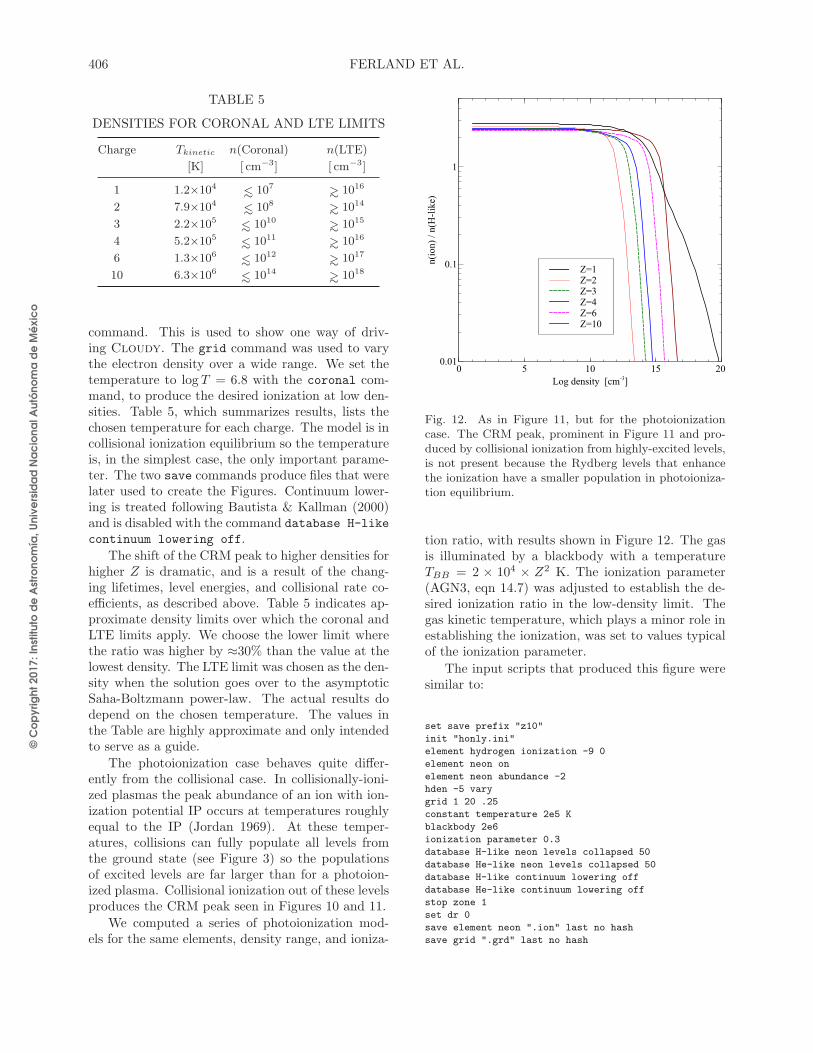
© C
op
yri
gh
t 2
01
7: In
stitu
to d
e A
stro
no
mía
, U
niv
ers
ida
d N
ac
ion
al A
utó
no
ma
de
Mé
xic
o
406 FERLAND ET AL.
TABLE 5
DENSITIES FOR CORONAL AND LTE LIMITS
Charge Tkinetic n(Coronal) n(LTE)
[K] [ cm−3] [ cm−3]
1 1.2×10⁴ ∼< 107 ∼> 1016
2 7.9×10⁴ ∼< 108 ∼> 1014
3 2.2×10⁵ ∼< 1010 ∼> 1015
4 5.2×10⁵ ∼< 1011 ∼> 1016
6 1.3×10⁶ ∼< 1012 ∼> 1017
10 6.3×10⁶ ∼< 1014 ∼> 1018
command. This is used to show one way of driv-ing Cloudy. The grid command was used to varythe electron density over a wide range. We set thetemperature to log T = 6.8 with the coronal com-mand, to produce the desired ionization at low den-sities. Table 5, which summarizes results, lists thechosen temperature for each charge. The model is incollisional ionization equilibrium so the temperatureis, in the simplest case, the only important parame-ter. The two save commands produce files that werelater used to create the Figures. Continuum lower-ing is treated following Bautista & Kallman (2000)and is disabled with the command database H-like
continuum lowering off.
The shift of the CRM peak to higher densities forhigher Z is dramatic, and is a result of the chang-ing lifetimes, level energies, and collisional rate co-efficients, as described above. Table 5 indicates ap-proximate density limits over which the coronal andLTE limits apply. We choose the lower limit wherethe ratio was higher by ≈30% than the value at thelowest density. The LTE limit was chosen as the den-sity when the solution goes over to the asymptoticSaha-Boltzmann power-law. The actual results dodepend on the chosen temperature. The values inthe Table are highly approximate and only intendedto serve as a guide.
The photoionization case behaves quite differ-ently from the collisional case. In collisionally-ioni-zed plasmas the peak abundance of an ion with ion-ization potential IP occurs at temperatures roughlyequal to the IP (Jordan 1969). At these temper-atures, collisions can fully populate all levels fromthe ground state (see Figure 3) so the populationsof excited levels are far larger than for a photoion-ized plasma. Collisional ionization out of these levelsproduces the CRM peak seen in Figures 10 and 11.
We computed a series of photoionization mod-els for the same elements, density range, and ioniza-
Fig. 12. As in Figure 11, but for the photoionizationcase. The CRM peak, prominent in Figure 11 and pro-duced by collisional ionization from highly-excited levels,is not present because the Rydberg levels that enhancethe ionization have a smaller population in photoioniza-tion equilibrium.
tion ratio, with results shown in Figure 12. The gasis illuminated by a blackbody with a temperatureTBB = 2 × 10⁴ × Z2 K. The ionization parameter(AGN3, eqn 14.7) was adjusted to establish the de-sired ionization ratio in the low-density limit. Thegas kinetic temperature, which plays a minor role inestablishing the ionization, was set to values typicalof the ionization parameter.
The input scripts that produced this figure weresimilar to:
set save prefix "z10"
init "honly.ini"
element hydrogen ionization -9 0
element neon on
element neon abundance -2
hden -5 vary
grid 1 20 .25
constant temperature 2e5 K
blackbody 2e6
ionization parameter 0.3
database H-like neon levels collapsed 50
database He-like neon levels collapsed 50
database H-like continuum lowering off
database He-like continuum lowering off
stop zone 1
set dr 0
save element neon ".ion" last no hash
save grid ".grd" last no hash
© C
op
yri
gh
t 2
01
7: In
stitu
to d
e A
stro
no
mía
, U
niv
ers
ida
d N
ac
ion
al A
utó
no
ma
de
Mé
xic
o
THE 2017 RELEASE OF Cloudy 407
TABLE 6
DENSITIES FOR PHOTOIONIZATIONCORONAL LIMIT
Charge Coronal
[ cm−3]
1 ∼< 1010
2 ∼< 1010
3 ∼< 1012
4 ∼< 1014
6 ∼< 1016
10 ∼< 1016
Many of the commands are similar to the collisionalionization case. This example shows a second wayto vary the electron density over the desired range.Only H and Ne are included in the model, and Nehas a modest abundance. The hydrogen ionizationfraction is set so that the H0 density is 10−9 smallerthan the total hydrogen density.
The CRM peak is not present because excitedlevels are not overpopulated at these lower temper-atures. The decreasing ionization at high densitiesis produced by three-body recombination bringinghigher levels into LTE. Table 6 gives the density limitfor the two-level approximation to be valid. This istaken as the density where the ionization ratio hasfallen by 30%. As also happened in Table 5, hy-drogen behaves differently because electron - atomcollision rate coefficients are so much smaller thanelectron-ion rate coefficients.
Tables 5 and 6 are meant as an indication ofwhere our methods of solving for the ionization ofmany-electron systems will fail. The ranges of valid-ity are highly approximate for several reasons. Thecollisional ionization results are sensitive to the gaskinetic temperature while the photoionization pre-dictions depend on the SED shape. Further, we onlyhave complete CRM models, extending to high Ry-dberg levels, for one and two-electron systems. Theenergy level structure, as shown in Figure 3, doesnot resemble the structure of many-electron systems,which tend to have a higher density of levels with lowenergies.
We are working to incorporate the CRM meth-ods developed by the laboratory plasma communityto have a better representation of the highly excitedlevels. A number of physics codes have been devel-oped, mainly in support of experimental facilities, todo just that. Many are summarized in the NLTE7and NLTE9 code-comparison workshop summaries
of Chung et al. (2013) and Piron et al. (2017). Fewof these codes are openly available. The ADAS datacollection, part of the ADAS code described by Sum-mers et al. (2006), is available through the OPEN-ADAS16 portal, and the FLYCHK code of Chunget al. (2005) is hosted at NIST17.
4. ATOMS AND IONS
The greatest changes to our treatment of atomsand ions involved the move to large databases, asdescribed in § 2, and the development of our Stoutdatabase (Lykins et al. 2015). This section describesother advances, mainly involving Gaunt factors.
Gaunt factors, named after John Arthur Gaunt,are corrections to classical electron-ion interactiontheory to incorporate quantum results (Garstang1993). Three Gaunt factors are encountered (Men-zel & Pekeris 1935; Aller 1963). Following the Men-zel & Pekeris (1935) numbering and Chandrasekhar’snotation (Chandrasekhar 1957), gI corrects bound-bound transitions, gII describes free-bound pro-cesses and is discussed in § 4.2 below, while gIIIadjusts free-free or bremsstrahlung emission and isdiscussed in the next section. Burgess & Summers(1987) summarize numerical methods of calculatingradiative Gaunt factors for complex ions.
4.1. Free-Free Gaunt Factor gIII
Free-free or bremsstrahlung emission is the dom-inant coolant at high temperatures, is usually themain contributor to radio emission in nebulae, andcan produce emission across the full electromagneticspectrum if the gas is hot enough. As Figure 5.2 ofRybicki & Lightman (1979) shows, different rangesof temperatures and photon energies require differentasymptotic expressions for gIII . These approxima-tions do not join continuously with one another. Forthis reason, it is not possible to use such expansionsacross the full temperature and spectral range wecover with Cloudy.
van Hoof et al. (2014) derived averaged andwavelength-specific free-free Gaunt factors gIII , lim-ited to non-relativistic energies. This work was ex-tended by van Hoof et al. (2015) to include pa-rameters where relativistic effects were important.Results from both studies were presented as tablesthat can be downloaded, and these are now used byCloudy to predict free-free emission.
Values of gIII covering the full range of kinetictemperature, photon energy, and nuclear charge con-sidered by Cloudy are shown in Figure 13. As is
16http://open.adas.ac.uk/17http://nlte.nist.gov/FLY/
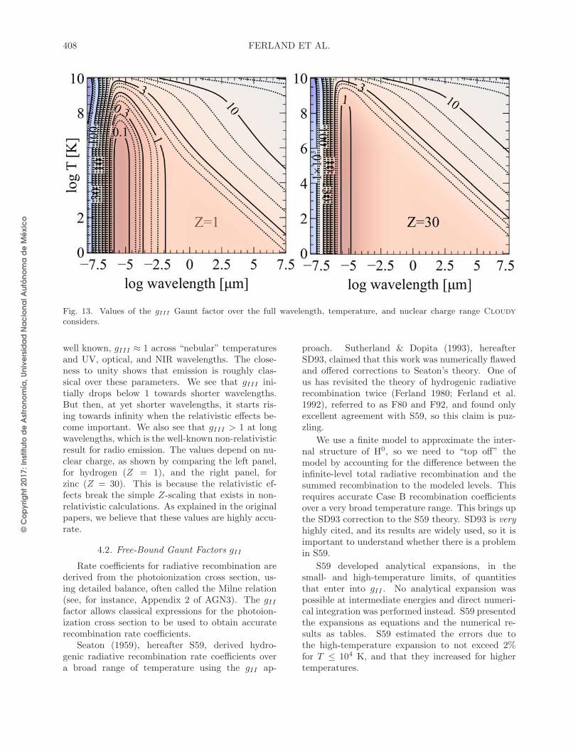
© C
op
yri
gh
t 2
01
7: In
stitu
to d
e A
stro
no
mía
, U
niv
ers
ida
d N
ac
ion
al A
utó
no
ma
de
Mé
xic
o
408 FERLAND ET AL.
Fig. 13. Values of the gIII Gaunt factor over the full wavelength, temperature, and nuclear charge range Cloudy
considers.
well known, gIII ≈ 1 across “nebular” temperaturesand UV, optical, and NIR wavelengths. The close-ness to unity shows that emission is roughly clas-sical over these parameters. We see that gIII ini-tially drops below 1 towards shorter wavelengths.But then, at yet shorter wavelengths, it starts ris-ing towards infinity when the relativistic effects be-come important. We also see that gIII > 1 at longwavelengths, which is the well-known non-relativisticresult for radio emission. The values depend on nu-clear charge, as shown by comparing the left panel,for hydrogen (Z = 1), and the right panel, forzinc (Z = 30). This is because the relativistic ef-fects break the simple Z-scaling that exists in non-relativistic calculations. As explained in the originalpapers, we believe that these values are highly accu-rate.
4.2. Free-Bound Gaunt Factors gII
Rate coefficients for radiative recombination arederived from the photoionization cross section, us-ing detailed balance, often called the Milne relation(see, for instance, Appendix 2 of AGN3). The gIIfactor allows classical expressions for the photoion-ization cross section to be used to obtain accuraterecombination rate coefficients.
Seaton (1959), hereafter S59, derived hydro-genic radiative recombination rate coefficients overa broad range of temperature using the gII ap-
proach. Sutherland & Dopita (1993), hereafterSD93, claimed that this work was numerically flawedand offered corrections to Seaton’s theory. One ofus has revisited the theory of hydrogenic radiativerecombination twice (Ferland 1980; Ferland et al.1992), referred to as F80 and F92, and found onlyexcellent agreement with S59, so this claim is puz-zling.
We use a finite model to approximate the inter-nal structure of H0, so we need to “top off” themodel by accounting for the difference between theinfinite-level total radiative recombination and thesummed recombination to the modeled levels. Thisrequires accurate Case B recombination coefficientsover a very broad temperature range. This brings upthe SD93 correction to the S59 theory. SD93 is veryhighly cited, and its results are widely used, so it isimportant to understand whether there is a problemin S59.
S59 developed analytical expansions, in thesmall- and high-temperature limits, of quantitiesthat enter into gII . No analytical expansion waspossible at intermediate energies and direct numeri-cal integration was performed instead. S59 presentedthe expansions as equations and the numerical re-sults as tables. S59 estimated the errors due tothe high-temperature expansion to not exceed 2%for T ≤ 104 K, and that they increased for highertemperatures.

© C
op
yri
gh
t 2
01
7: In
stitu
to d
e A
stro
no
mía
, U
niv
ers
ida
d N
ac
ion
al A
utó
no
ma
de
Mé
xic
o
THE 2017 RELEASE OF Cloudy 409
Fig. 14. This shows two of the quantities that enter intothe S59 calculation of gII . The vertical dotted line marksthe point where SD93 claim that Seaton’s theory is dis-continuous. The dashed-dotted lines give the quantitiesplotted in the lower panel of Figure 1 of SD93. Thedashed curves give SD93’s “corrected Seaton” theory.The heavy solid lines give our recalculation of the termsS and σ using Seaton’s original expressions and tables.
SD93, § 3.4.1 and Figure 1, report that theS59 intermediate-temperature numerical, and high-temperature analytical, results do not smoothly joinone another, and offer an alternative expression forthe high-temperature part. We show results fromtheir tables and figure as our Figures 14 and 15.Figure 14 shows one of the S59 intermediate re-sults taken from their tables. The line marked“SD93 Seaton” is their version of S59 while “cor-rected Seaton” is their altered version. F80 closelyfollowed S59, so we have some experience in workingwith this paper. The heavy line is our evaluation ofS59. It is continuous and somewhat displaced fromSD93.
Figure 15 compares total recombination rate co-efficients over the narrow temperature range whereSD93 report problems. The discontinuities are obvi-
Fig. 15. Hydrogenic recombination rate coefficients areshown vs. reduced temperature, T/Z2, for the groundstate, n = 1. The vertical dotted line marks the SD93discontinuity, where the theory changes from the nu-merical to analytical forms. The dash-dotted line givesSD93’s evaluation of the Seaton rate, taken from the up-per panel of their Figure 1. The dashed line is SD93’s“corrected Seaton” theory. The heavy solid line givesour recalculation of the rates using Seaton’s original ex-pressions and tables. All the rates are multiplied by thereduced temperature.
ous. The heavy line is our evaluation of S59. It iscontinuous and displaced from SD93.
Figure 16 shows total recombination rate coeffi-cients over a broad range of temperature. The heavyline gives our reevaluation of the Seaton results. S59notes that his expressions are not valid above 106 Kand the heavy line ends at that temperature. Thelines marked “Mappings I” and “corrected Seaton”are taken from SD93. The line marked “Mappings I”is an extrapolation of the S59 expression as used byArnaud & Rothenflug (1985) and the Mappings Icode. The line marked “corrected Seaton” is the ex-pression proposed by SD93.
Today the gII approach is seldom used becauselarge repositories of photoionization cross-sections,such as the Opacity Project (Seaton 1987), are read-ily available, so the Milne relation can be applieddirectly to photoionization cross sections. F92 tookthis approach. The F92 results are believed to beof high accuracy for all temperatures presented, aswas recently confirmed by Mao et al. (2017). S59 re-ported that his results should be “in error by lessthan 0.5 per cent for (T/Z2) ≤ 105 K, by 3 percent for (T/Z2) = 106 K and by 31 per cent for(T/Z2) = 5× 10⁶ K.” F92 confirms these error esti-mates.
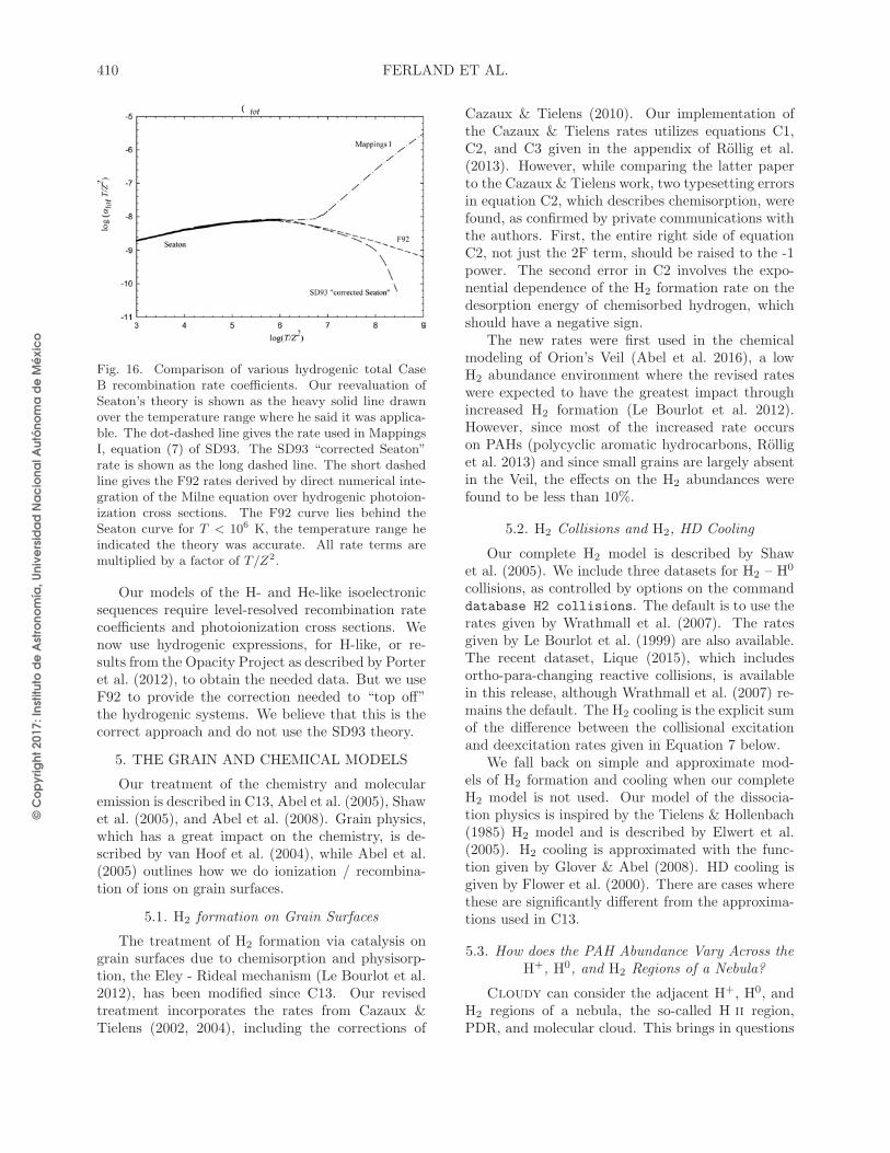
© C
op
yri
gh
t 2
01
7: In
stitu
to d
e A
stro
no
mía
, U
niv
ers
ida
d N
ac
ion
al A
utó
no
ma
de
Mé
xic
o
410 FERLAND ET AL.
Fig. 16. Comparison of various hydrogenic total CaseB recombination rate coefficients. Our reevaluation ofSeaton’s theory is shown as the heavy solid line drawnover the temperature range where he said it was applica-ble. The dot-dashed line gives the rate used in MappingsI, equation (7) of SD93. The SD93 “corrected Seaton”rate is shown as the long dashed line. The short dashedline gives the F92 rates derived by direct numerical inte-gration of the Milne equation over hydrogenic photoion-ization cross sections. The F92 curve lies behind theSeaton curve for T < 106 K, the temperature range heindicated the theory was accurate. All rate terms aremultiplied by a factor of T/Z2.
Our models of the H- and He-like isoelectronicsequences require level-resolved recombination ratecoefficients and photoionization cross sections. Wenow use hydrogenic expressions, for H-like, or re-sults from the Opacity Project as described by Porteret al. (2012), to obtain the needed data. But we useF92 to provide the correction needed to “top off”the hydrogenic systems. We believe that this is thecorrect approach and do not use the SD93 theory.
5. THE GRAIN AND CHEMICAL MODELS
Our treatment of the chemistry and molecularemission is described in C13, Abel et al. (2005), Shawet al. (2005), and Abel et al. (2008). Grain physics,which has a great impact on the chemistry, is de-scribed by van Hoof et al. (2004), while Abel et al.(2005) outlines how we do ionization / recombina-tion of ions on grain surfaces.
5.1. H2 formation on Grain Surfaces
The treatment of H2 formation via catalysis ongrain surfaces due to chemisorption and physisorp-tion, the Eley - Rideal mechanism (Le Bourlot et al.2012), has been modified since C13. Our revisedtreatment incorporates the rates from Cazaux &Tielens (2002, 2004), including the corrections of
Cazaux & Tielens (2010). Our implementation ofthe Cazaux & Tielens rates utilizes equations C1,C2, and C3 given in the appendix of Rollig et al.(2013). However, while comparing the latter paperto the Cazaux & Tielens work, two typesetting errorsin equation C2, which describes chemisorption, werefound, as confirmed by private communications withthe authors. First, the entire right side of equationC2, not just the 2F term, should be raised to the -1power. The second error in C2 involves the expo-nential dependence of the H2 formation rate on thedesorption energy of chemisorbed hydrogen, whichshould have a negative sign.
The new rates were first used in the chemicalmodeling of Orion’s Veil (Abel et al. 2016), a lowH2 abundance environment where the revised rateswere expected to have the greatest impact throughincreased H2 formation (Le Bourlot et al. 2012).However, since most of the increased rate occurson PAHs (polycyclic aromatic hydrocarbons, Rolliget al. 2013) and since small grains are largely absentin the Veil, the effects on the H2 abundances werefound to be less than 10%.
5.2. H2 Collisions and H2, HD Cooling
Our complete H2 model is described by Shawet al. (2005). We include three datasets for H2 – H0
collisions, as controlled by options on the commanddatabase H2 collisions. The default is to use therates given by Wrathmall et al. (2007). The ratesgiven by Le Bourlot et al. (1999) are also available.The recent dataset, Lique (2015), which includesortho-para-changing reactive collisions, is availablein this release, although Wrathmall et al. (2007) re-mains the default. The H2 cooling is the explicit sumof the difference between the collisional excitationand deexcitation rates given in Equation 7 below.
We fall back on simple and approximate mod-els of H2 formation and cooling when our completeH2 model is not used. Our model of the dissocia-tion physics is inspired by the Tielens & Hollenbach(1985) H2 model and is described by Elwert et al.(2005). H2 cooling is approximated with the func-tion given by Glover & Abel (2008). HD cooling isgiven by Flower et al. (2000). There are cases wherethese are significantly different from the approxima-tions used in C13.
5.3. How does the PAH Abundance Vary Across theH+, H0, and H2 Regions of a Nebula?
Cloudy can consider the adjacent H+, H0, andH2 regions of a nebula, the so-called H ii region,PDR, and molecular cloud. This brings in questions
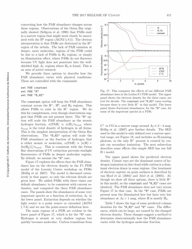
© C
op
yri
gh
t 2
01
7: In
stitu
to d
e A
stro
no
mía
, U
niv
ers
ida
d N
ac
ion
al A
utó
no
ma
de
Mé
xic
o
THE 2017 RELEASE OF Cloudy 411
concerning how the PAH abundance changes acrossthese regions. Observations of the Orion Bar origi-nally showed (Sellgren et al. 1990) that PAHs emitin a narrow region that might most closely be associ-ated with the H0 region (AGN3 § 8.5). The obviousinterpretation is that PAHs are destroyed in the H+
region of the nebula. The lack of PAH emission atdeeper, more molecular, regions of the PDR couldbe due to a lack of PAHs in H2 regions, or simplyan illumination effect, where PAHs do not fluorescebecause UV light does not penetrate into the well-shielded high AV regions where H2 is found. This isan area of active research
We provide three options to describe how thePAH abundance varies with physical conditions.These are controlled with the commands:
set PAH constant
set PAH "H"
set PAH "H,H2"
The constant option will keep the PAH abundanceconstant across the H+, H0, and H2 regions. Thisallows PAHs to exist in the H+ region. We dothis for completeness, even though observations sug-gest that PAHs are not present there. The "H" op-tion will scale the PAH abundance as the atomichydrogen fraction, n(PAH) ∝ n(H)/ntotal, wherentotal is the total density of hydrogen in all forms.This is the simplest interpretation of the Orion Barobservations. The "H,H2" option will scale thePAH abundance as the fraction of hydrogen thatis either atomic or molecular, n(PAH) ∝ [n(H) +2n(H2))]/ntotal. This is consistent with the OrionBar observations if UV extinction prevents starlightfluorescence of PAHs in deeper molecular regions.By default, we assume the "H" case.
Figure 17 explores the effects that the PAH abun-dance has on the electron density in the F1 PDRmodel of the Lorentz Center workshop on PDRs(Rollig et al. 2007). The model is discussed exten-sively in that paper, so only the relevant details aregiven here. We added PAHs with three times ourdefault abundance, to be consistent with current es-timates, and computed the three PAH abundancecases. The panels show the abundances of some veryimportant species as a function of extinction AV inthe lower panel. Extinction depends on whether thelight source is a point source or extended (AGN3§ 7.6) and we use the point-source definition here.
The main regions of a PDR are evident in thelower panel of Figure 17, which is for the "H" case.Hydrogen is atomic at very shallow regions butquickly becomes molecular. Carbon transitions from
Fig. 17. This compares the effects of our different PAHabundance laws in the Leiden F1 PDR model. The upperpanel shows the electron density for the three cases, seetext for details. The constant and "H,H2" cases overlapbecause there is very little H+ in this model. The lowerpanel shows fractional abundances, for the "H" case, forsome of the important species in a PDR.
C+ to CO in a narrow range around AV ≈ 2−4 mag.Rollig et al. (2007) give further details. The SEDused in this model is only defined over a narrow spec-tral range, see Figure 18, and includes no H-ionizingphotons, so the only H+ present is created by cos-mic ray secondary ionization. The next subsectiondescribes some effects this simple SED has our fullH i model.
The upper panel shows the predicted electrondensity. Cosmic rays are the dominant source of hy-drogen ionization in this cloud while carbon is a dom-inant electron donor in some regions. Our treatmentof electron capture on grain surfaces is described byvan Hoof et al. (2004) and Abel et al. (2005). Al-though we show all three options, there is little H+
in this model, so the constant and "H,H2" cases areidentical. The PAH abundance does not vary acrossFigure 17 in that case. In the "H" case, PAHs arepresent near the illuminated face but have very lowabundance at AV > 1 mag, where H is mostly H2.
Table 7 shows the logs of some predicted columndensities for the "H,H2" and "H" cases. The differ-ences, which can be large, are caused by the changedelectron density. These changes suggest a method todetermine observationally how the PAH abundancevaries with the hydrogen molecular fraction.
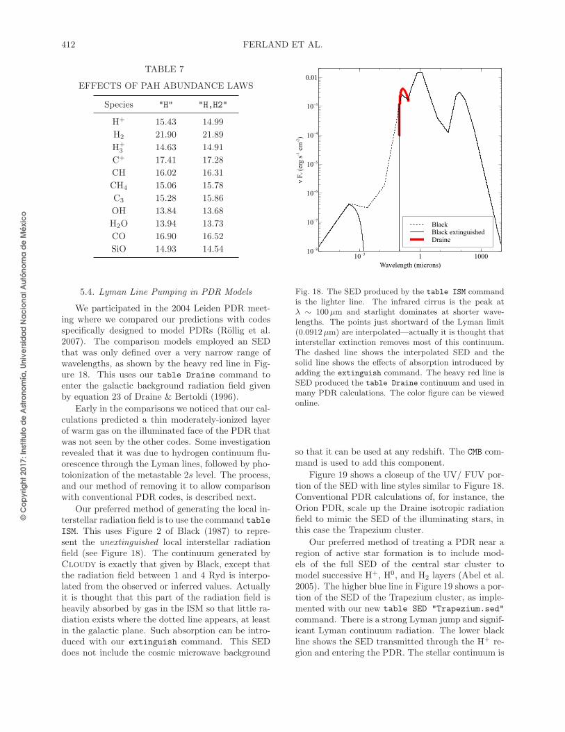
© C
op
yri
gh
t 2
01
7: In
stitu
to d
e A
stro
no
mía
, U
niv
ers
ida
d N
ac
ion
al A
utó
no
ma
de
Mé
xic
o
412 FERLAND ET AL.
TABLE 7
EFFECTS OF PAH ABUNDANCE LAWS
Species "H" "H,H2"
H+ 15.43 14.99
H2 21.90 21.89
H+3 14.63 14.91
C+ 17.41 17.28
CH 16.02 16.31
CH4 15.06 15.78
C3 15.28 15.86
OH 13.84 13.68
H2O 13.94 13.73
CO 16.90 16.52
SiO 14.93 14.54
5.4. Lyman Line Pumping in PDR Models
We participated in the 2004 Leiden PDR meet-ing where we compared our predictions with codesspecifically designed to model PDRs (Rollig et al.2007). The comparison models employed an SEDthat was only defined over a very narrow range ofwavelengths, as shown by the heavy red line in Fig-ure 18. This uses our table Draine command toenter the galactic background radiation field givenby equation 23 of Draine & Bertoldi (1996).
Early in the comparisons we noticed that our cal-culations predicted a thin moderately-ionized layerof warm gas on the illuminated face of the PDR thatwas not seen by the other codes. Some investigationrevealed that it was due to hydrogen continuum flu-orescence through the Lyman lines, followed by pho-toionization of the metastable 2s level. The process,and our method of removing it to allow comparisonwith conventional PDR codes, is described next.
Our preferred method of generating the local in-terstellar radiation field is to use the command table
ISM. This uses Figure 2 of Black (1987) to repre-sent the unextinguished local interstellar radiationfield (see Figure 18). The continuum generated byCloudy is exactly that given by Black, except thatthe radiation field between 1 and 4 Ryd is interpo-lated from the observed or inferred values. Actuallyit is thought that this part of the radiation field isheavily absorbed by gas in the ISM so that little ra-diation exists where the dotted line appears, at leastin the galactic plane. Such absorption can be intro-duced with our extinguish command. This SEDdoes not include the cosmic microwave background
Fig. 18. The SED produced by the table ISM commandis the lighter line. The infrared cirrus is the peak atλ ∼ 100µm and starlight dominates at shorter wave-lengths. The points just shortward of the Lyman limit(0.0912µm) are interpolated—actually it is thought thatinterstellar extinction removes most of this continuum.The dashed line shows the interpolated SED and thesolid line shows the effects of absorption introduced byadding the extinguish command. The heavy red line isSED produced the table Draine continuum and used inmany PDR calculations. The color figure can be viewedonline.
so that it can be used at any redshift. The CMB com-mand is used to add this component.
Figure 19 shows a closeup of the UV/ FUV por-tion of the SED with line styles similar to Figure 18.Conventional PDR calculations of, for instance, theOrion PDR, scale up the Draine isotropic radiationfield to mimic the SED of the illuminating stars, inthis case the Trapezium cluster.
Our preferred method of treating a PDR near aregion of active star formation is to include mod-els of the full SED of the central star cluster tomodel successive H+, H0, and H2 layers (Abel et al.2005). The higher blue line in Figure 19 shows a por-tion of the SED of the Trapezium cluster, as imple-mented with our new table SED "Trapezium.sed"
command. There is a strong Lyman jump and signif-icant Lyman continuum radiation. The lower blackline shows the SED transmitted through the H+ re-gion and entering the PDR. The stellar continuum is
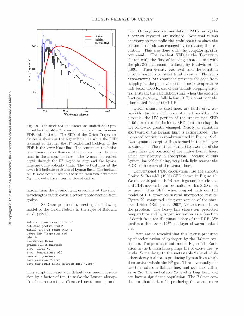
© C
op
yri
gh
t 2
01
7: In
stitu
to d
e A
stro
no
mía
, U
niv
ers
ida
d N
ac
ion
al A
utó
no
ma
de
Mé
xic
o
THE 2017 RELEASE OF Cloudy 413
Fig. 19. The thick red line shows the limited SED pro-duced by the table Draine command and used in manyPDR calculations. The SED of the Orion Trapeziumcluster is shown as the higher blue line while the SEDtransmitted through the H+ region and incident on thePDR is the lower black line. The continuum resolutionis ten times higher than our default to increase the con-trast in the absorption lines. The Lyman line opticaldepth through the H+ region is large and the Lymanlines are quite optically thick. The vertical lines at thelower left indicate positions of Lyman lines. The incidentSEDs were normalized to the same radiation parameterG0. The color figure can be viewed online.
harder than the Draine field, especially at the shortwavelengths which cause electron photoejection fromgrains.
This SED was produced by creating the followingmodel of the Orion Nebula in the style of Baldwinet al. (1991):
set continuum resolution 0.1
set save prefix "full"
phi(H) 13.0721 range 0.25 1
table SED "Trapezium.sed"
hden 4
abundances Orion
grains PAH 3 function
stop efrac -2
stop temperature off
constant pressure
save overview ".ovr"
save continuum units microns last ".con"
This script increases our default continuum resolu-tion by a factor of ten, to make the Lyman absorp-tion line contrast, as discussed next, more promi-
nent. Orion grains and our default PAHs, using thefunction keyword, are included. Note that it wasnecessary to recompile the grain opacities since thecontinuum mesh was changed by increasing the res-olution. This was done with the compile grains
command. The incident SED is the Trapeziumcluster with the flux of ionizing photons, set withthe phi(H) command, deduced by Baldwin et al.(1991). Their density was used, and the equationof state assumes constant total pressure. The stop
temperature off command prevents the code fromstopping at the point where the kinetic temperaturefalls below 4000 K, one of our default stopping crite-ria. Instead, the calculation stops when the electronfraction, ne/ntotal, falls below 10−2, a point near theilluminated face of the PDR.
Orion grains, as used here, are fairly grey, ap-parently due to a deficiency of small particles. Asa result, the UV portion of the transmitted SEDis fainter than the incident SED, but the shape isnot otherwise greatly changed. Nearly all radiationshortward of the Lyman limit is extinguished. Theincreased continuum resolution used in Figure 19 al-lows Lyman absorption lines formed in the H+ layerto stand out. The vertical bars at the lower left of thefigure mark the positions of the higher Lyman lines,which are strongly in absorption. Because of thisLyman line self-shielding, very little light reaches thePDR in the cores of the Lyman lines.
Conventional PDR calculations use the smoothDraine & Bertoldi (1996) SED shown in Figure 19.We do participate in PDR meetings and include sev-eral PDR models in our test suite, so this SED mustbe used. This SED, when coupled with our fullmodel of H i, produces several unexpected results.Figure 20, computed using our version of the stan-dard Leiden (Rollig et al. 2007) V4 test case, showsthe problem. The heavy line shows our predictedtemperature and hydrogen ionization as a functionof depth from the illuminated face of the PDR. Wepredict a thin, δr ∼ 1010 cm, layer of warm ionizedgas.
Examination revealed that this layer is producedby photoionization of hydrogen by the Balmer con-tinuum. The process is outlined in Figure 21. Radi-ation in the Lyman lines pumps H i to excite the nplevels. Some decay to the metastable 2s level whileothers decay back to 1s producing Lyman lines whichthen scatter within the H0 gas. These eventually de-cay to produce a Balmer line, and populate either2s or 2p. The metastable 2s level is long lived andcan have a significant population. The Balmer con-tinuum photoionizes 2s, producing the warm, more

© C
op
yri
gh
t 2
01
7: In
stitu
to d
e A
stro
no
mía
, U
niv
ers
ida
d N
ac
ion
al A
utó
no
ma
de
Mé
xic
o
414 FERLAND ET AL.
Fig. 20. The gas kinetic temperature (upper panel) andionized hydrogen fraction (lower panel) for one of the Lei-den Meeting test cases. The thick line shows predictionsfor the simple PDR SED striking an unshielded PDR. Athin layer of warm ionized gas, produced by the processsketched in Figure 21, is produced. The thin line is thesame calculation but with the database H-like Lyman
pumping off command included to block Lyman line flu-orescence, as is done in the pdr leiden v4.in test casein our test suite.
ionized, layer. The thickness of the layer is set bythe column density needed for the Lyman lines tobecome self shielded.
In previous versions of Cloudy, we recom-mended adding the case B command to artificiallymake the Lyman lines optically thick. That com-mand has other effects and we introduce a newcommand, database H-like Lyman pumping off,to make all Lyman lines optically thick. The actualeffect is to prevent the pumping rather than changethe radiative transfer of the Lyman lines. When thiscommand is included in the input deck we obtain theresults shown as the light line in Figure 19. This notonly makes our predictions more closely match thoseof conventional PDR codes, but also results in a sig-nificant time savings since resolving the thin warmlayer is fairly expensive.
5.5. The LAMDA Database
Since C13, we have updated our version of theLAMDA (Schoier et al. 2005) database of molecularstructure and emission. LAMDA does not use ver-sion numbers. Our version of LAMDA was down-loaded on 2015 June 30.
In addition to updating collisional rates for sev-eral species, which have been modified by LAMDA
Fig. 21. This shows the process which produces the thinwarm layer in Figure 20. Radiation in the Lyman linesphotoexcites the np levels via high-n Lyman lines. Manydecay to the metastable 2s level, which is then photoion-ized by the Balmer continuum. The process is an artifactof the smooth SED used in PDR simulations. In nature,there is sufficient H i column density in the H+ layer tomake the Lyman lines self shielded.
since the last integration of Cloudy with theLAMDA database in C10, we added the ability topredict the intensity of five of their new species:OH+, H2S, H2CS, C2H, and NH2D.
Cloudy uses the stored level energies to pre-dict line wavelengths, photon energies, and collisionrates (Lykins et al. 2015). Some of the energy levelspresent in LAMDA are not precise enough to com-pute wavelengths with sufficient accuracy. LAMDAdoes give the frequency of all transitions to higherprecision than the energy levels. Therefore, for thespecies where more precision is needed, we modi-fied the LAMDA data to include higher precision forthe energy levels. This was especially important forhyperfine transitions, such as in OH, where comput-ing the wavelengths using the energy level spacingpresent in LAMDA leads to multiple transitions hav-ing the same wavelength. For C17, these issues havebeen resolved and all hyperfine transitions for OHare now specified with unique wavelengths.
Overall, the improved rates from the LAMDAupdate did change some molecular intensities in ourtest suite of simulations. The largest and most no-table were H2O, CS, and some of the high rotationaltransitions of CO.
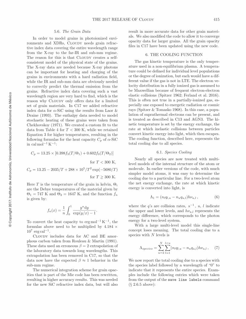
© C
op
yri
gh
t 2
01
7: In
stitu
to d
e A
stro
no
mía
, U
niv
ers
ida
d N
ac
ion
al A
utó
no
ma
de
Mé
xic
o
THE 2017 RELEASE OF Cloudy 415
5.6. The Grain Data
In order to model grains in photoionized envi-ronments and XDRs, Cloudy needs grain refrac-tive index data covering the entire wavelength rangefrom the X-ray to the far-IR and sub-mm regime.The reason for this is that Cloudy creates a self-consistent model of the physical state of the grains.The X-ray data are needed because X-ray photonscan be important for heating and charging of thegrains in environments with a hard radiation field,while the IR and sub-mm data are obviously neededto correctly predict the thermal emission from thegrains. Refractive index data covering such a vastwavelength region are very hard to find, which is thereason why Cloudy only offers data for a limitedset of grain materials. In C17 we added refractiveindex data for α-SiC using the results from Laor &Draine (1993). The enthalpy data needed to modelstochastic heating of these grains were taken fromChekhovskoy (1971). We created a custom fit to thedata from Table 4 for T < 300 K, while we retainedEquation 3 for higher temperatures, resulting in thefollowing formulas for the heat capacity Cp of α-SiCin calmol−1 K−1:
Cp = 13.25× [0.398f3(T/Θ1) + 0.602f3(T/Θ2)]
for T < 300 K,
Cp = 13.25− 2035/T + 288× 105/T 2 exp(−5680/T )
for T ≥ 300 K.
Here T is the temperature of the grain in kelvin, Θi
are the Debye temperatures of the material given byΘ1 = 747 K and Θ2 = 1647 K, and the function fnis given by:
fn(x) =1
n
∫ 1
0
yndy
exp(y/x)− 1.
To convert the heat capacity to ergmol−1 K−1, theformulas above need to be multiplied by 4.184 ×
107 erg cal−1.Cloudy includes data for AC and BE amor-
phous carbon taken from Rouleau & Martin (1991).These data used an erroneous β = 2 extrapolation ofthe laboratory data towards long wavelengths. Thisextrapolation has been removed in C17, so that thedata now have the expected β ≈ 1 behavior in thesub-mm regime.
The numerical integration scheme for grain opac-ities that is part of the Mie code has been rewritten,resulting in higher accuracy results. This was neededfor the new SiC refractive index data, but will also
result in more accurate data for other grain materi-als. We also modified the code to allow it to convergeopacity data for larger grains. All the grain opacityfiles in C17 have been updated using the new code.
6. THE COOLING FUNCTION
The gas kinetic temperature is the only temper-ature used in a non-equilibrium plasma. A tempera-ture could be defined for individual level populationsor the degree of ionization, but each would have a dif-ferent value if the gas is not in LTE. The electron ve-locity distribution in a fully ionized gas is assumed tobe Maxwellian because of frequent electron-electronelastic collisions (Spitzer 1962; Ferland et al. 2016).This is often not true in a partially-ionized gas, es-pecially one exposed to energetic radiation or cosmicrays (Spitzer & Tomasko 1968). In this case, a popu-lation of suprathermal electrons can be present, andis treated as described in C13 and AGN3. The ki-netic temperature is set by the energy exchange, therate at which inelastic collisions between particlesconvert kinetic energy into light, which then escapes.The cooling function, described here, represents thetotal cooling due to all species.
6.1. Species Cooling
Nearly all species are now treated with multi-level models of the internal structure of the atom ormolecule. In earlier versions of the code, with muchsimpler model atoms, it was easy to determine thecooling due to a particular line. For a two-level atomthe net energy exchange, the rate at which kineticenergy is converted into light, is
Λ1 = (nlql,u − nuqu,l)hνu,l , (6)
where the q’s are collision rates, s−1 , u, l indicatethe upper and lower levels, and hνu,l represents theenergy difference, which corresponds to the photonenergy for a two-level system.
With a large multi-level model this single-lineconcept loses meaning. The total cooling due to aspecies with N levels is
Λspecies =
N∑u=2
l<u∑l=1
(nlql,u − nuqu,l)hνu,l , (7)
We now report the total cooling due to a species withthe species label followed by a wavelength of “0” toindicate that it represents the entire species. Exam-ples include the following entries which were takenfrom the output of the save line labels command(§ 2.6.5 above):
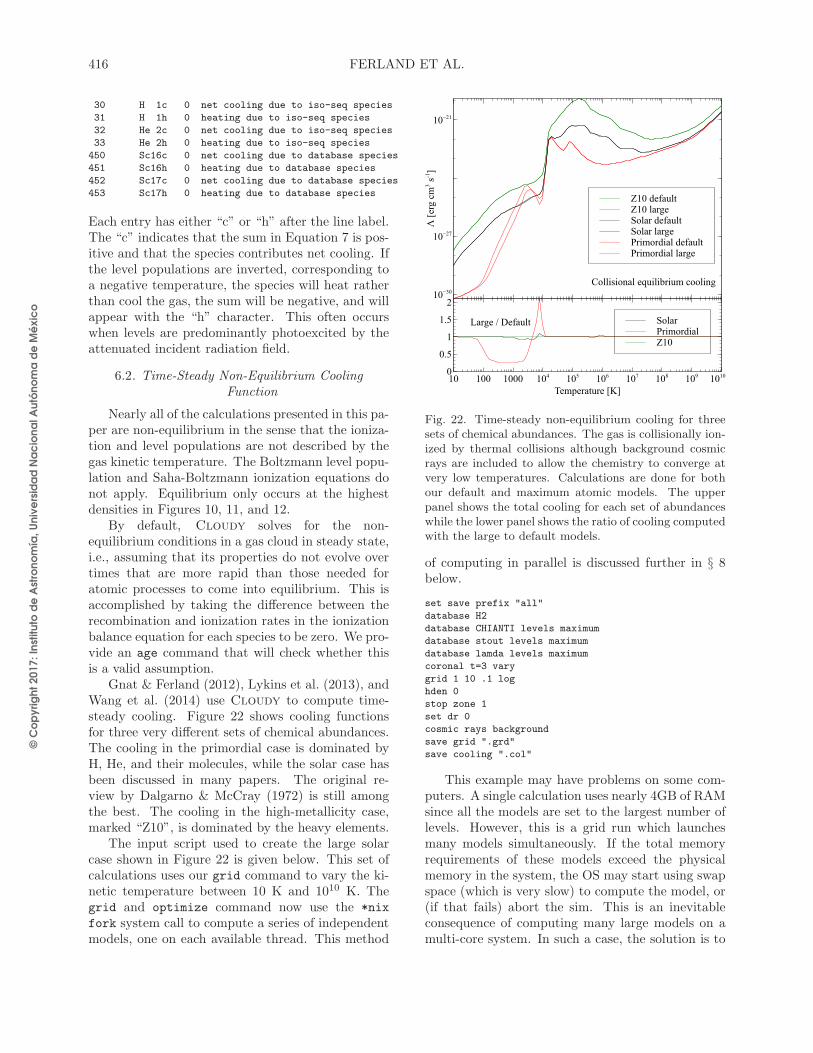
© C
op
yri
gh
t 2
01
7: In
stitu
to d
e A
stro
no
mía
, U
niv
ers
ida
d N
ac
ion
al A
utó
no
ma
de
Mé
xic
o
416 FERLAND ET AL.
30 H 1c 0 net cooling due to iso-seq species
31 H 1h 0 heating due to iso-seq species
32 He 2c 0 net cooling due to iso-seq species
33 He 2h 0 heating due to iso-seq species
450 Sc16c 0 net cooling due to database species
451 Sc16h 0 heating due to database species
452 Sc17c 0 net cooling due to database species
453 Sc17h 0 heating due to database species
Each entry has either “c” or “h” after the line label.The “c” indicates that the sum in Equation 7 is pos-itive and that the species contributes net cooling. Ifthe level populations are inverted, corresponding toa negative temperature, the species will heat ratherthan cool the gas, the sum will be negative, and willappear with the “h” character. This often occurswhen levels are predominantly photoexcited by theattenuated incident radiation field.
6.2. Time-Steady Non-Equilibrium CoolingFunction
Nearly all of the calculations presented in this pa-per are non-equilibrium in the sense that the ioniza-tion and level populations are not described by thegas kinetic temperature. The Boltzmann level popu-lation and Saha-Boltzmann ionization equations donot apply. Equilibrium only occurs at the highestdensities in Figures 10, 11, and 12.
By default, Cloudy solves for the non-equilibrium conditions in a gas cloud in steady state,i.e., assuming that its properties do not evolve overtimes that are more rapid than those needed foratomic processes to come into equilibrium. This isaccomplished by taking the difference between therecombination and ionization rates in the ionizationbalance equation for each species to be zero. We pro-vide an age command that will check whether thisis a valid assumption.
Gnat & Ferland (2012), Lykins et al. (2013), andWang et al. (2014) use Cloudy to compute time-steady cooling. Figure 22 shows cooling functionsfor three very different sets of chemical abundances.The cooling in the primordial case is dominated byH, He, and their molecules, while the solar case hasbeen discussed in many papers. The original re-view by Dalgarno & McCray (1972) is still amongthe best. The cooling in the high-metallicity case,marked “Z10”, is dominated by the heavy elements.
The input script used to create the large solarcase shown in Figure 22 is given below. This set ofcalculations uses our grid command to vary the ki-netic temperature between 10 K and 1010 K. Thegrid and optimize command now use the *nix
fork system call to compute a series of independentmodels, one on each available thread. This method
Fig. 22. Time-steady non-equilibrium cooling for threesets of chemical abundances. The gas is collisionally ion-ized by thermal collisions although background cosmicrays are included to allow the chemistry to converge atvery low temperatures. Calculations are done for bothour default and maximum atomic models. The upperpanel shows the total cooling for each set of abundanceswhile the lower panel shows the ratio of cooling computedwith the large to default models.
of computing in parallel is discussed further in § 8below.
set save prefix "all"
database H2
database CHIANTI levels maximum
database stout levels maximum
database lamda levels maximum
coronal t=3 vary
grid 1 10 .1 log
hden 0
stop zone 1
set dr 0
cosmic rays background
save grid ".grd"
save cooling ".col"
This example may have problems on some com-puters. A single calculation uses nearly 4GB of RAMsince all the models are set to the largest number oflevels. However, this is a grid run which launchesmany models simultaneously. If the total memoryrequirements of these models exceed the physicalmemory in the system, the OS may start using swapspace (which is very slow) to compute the model, or(if that fails) abort the sim. This is an inevitableconsequence of computing many large models on amulti-core system. In such a case, the solution is to
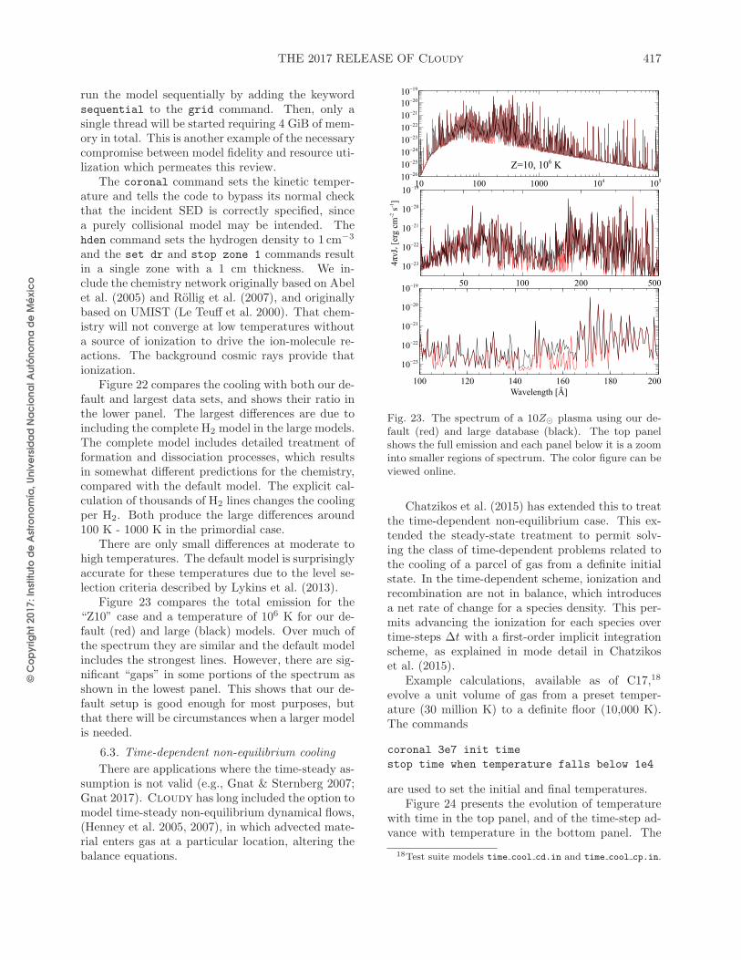
© C
op
yri
gh
t 2
01
7: In
stitu
to d
e A
stro
no
mía
, U
niv
ers
ida
d N
ac
ion
al A
utó
no
ma
de
Mé
xic
o
THE 2017 RELEASE OF Cloudy 417
run the model sequentially by adding the keywordsequential to the grid command. Then, only asingle thread will be started requiring 4 GiB of mem-ory in total. This is another example of the necessarycompromise between model fidelity and resource uti-lization which permeates this review.
The coronal command sets the kinetic temper-ature and tells the code to bypass its normal checkthat the incident SED is correctly specified, sincea purely collisional model may be intended. Thehden command sets the hydrogen density to 1 cm−3
and the set dr and stop zone 1 commands resultin a single zone with a 1 cm thickness. We in-clude the chemistry network originally based on Abelet al. (2005) and Rollig et al. (2007), and originallybased on UMIST (Le Teuff et al. 2000). That chem-istry will not converge at low temperatures withouta source of ionization to drive the ion-molecule re-actions. The background cosmic rays provide thationization.
Figure 22 compares the cooling with both our de-fault and largest data sets, and shows their ratio inthe lower panel. The largest differences are due toincluding the complete H2 model in the large models.The complete model includes detailed treatment offormation and dissociation processes, which resultsin somewhat different predictions for the chemistry,compared with the default model. The explicit cal-culation of thousands of H2 lines changes the coolingper H2. Both produce the large differences around100 K - 1000 K in the primordial case.
There are only small differences at moderate tohigh temperatures. The default model is surprisinglyaccurate for these temperatures due to the level se-lection criteria described by Lykins et al. (2013).
Figure 23 compares the total emission for the“Z10” case and a temperature of 106 K for our de-fault (red) and large (black) models. Over much ofthe spectrum they are similar and the default modelincludes the strongest lines. However, there are sig-nificant “gaps” in some portions of the spectrum asshown in the lowest panel. This shows that our de-fault setup is good enough for most purposes, butthat there will be circumstances when a larger modelis needed.
6.3. Time-dependent non-equilibrium cooling
There are applications where the time-steady as-sumption is not valid (e.g., Gnat & Sternberg 2007;Gnat 2017). Cloudy has long included the option tomodel time-steady non-equilibrium dynamical flows,(Henney et al. 2005, 2007), in which advected mate-rial enters gas at a particular location, altering thebalance equations.
Fig. 23. The spectrum of a 10Z⊙ plasma using our de-fault (red) and large database (black). The top panelshows the full emission and each panel below it is a zoominto smaller regions of spectrum. The color figure can beviewed online.
Chatzikos et al. (2015) has extended this to treatthe time-dependent non-equilibrium case. This ex-tended the steady-state treatment to permit solv-ing the class of time-dependent problems related tothe cooling of a parcel of gas from a definite initialstate. In the time-dependent scheme, ionization andrecombination are not in balance, which introducesa net rate of change for a species density. This per-mits advancing the ionization for each species overtime-steps ∆t with a first-order implicit integrationscheme, as explained in mode detail in Chatzikoset al. (2015).
Example calculations, available as of C17,18
evolve a unit volume of gas from a preset temper-ature (30 million K) to a definite floor (10,000 K).The commands
coronal 3e7 init time
stop time when temperature falls below 1e4
are used to set the initial and final temperatures.Figure 24 presents the evolution of temperature
with time in the top panel, and of the time-step ad-vance with temperature in the bottom panel. The
18Test suite models time cool cd.in and time cool cp.in.

© C
op
yri
gh
t 2
01
7: In
stitu
to d
e A
stro
no
mía
, U
niv
ers
ida
d N
ac
ion
al A
utó
no
ma
de
Mé
xic
o
418 FERLAND ET AL.
104
105
106
107
108
101 102
Tem
pera
ture
/ K
Time / Myr
� = const
� = const, CIE
P = const
P = const, CIE
10-1
100
101
102
103
104
105
106
107
104 105 106 107
�
t / yr
Temperature / K
✁ = const
✁ = const, CIE
P = const
P = const, CIE
Fig. 24. Time-dependent cooling of a unit volume ofgas. Evolution of temperature with time (top panel) andtime-step advance with temperature (bottom panel) un-der isobaric and isochoric conditions. The dashed curvesshow the evolution assuming collisional ionization equi-librium (CIE). The color figure can be viewed online.
solver adapts the time-step to track the changingconditions in the gas. At high temperatures, the sys-tem evolves slowly, and large time-steps are taken,while at lower temperatures, the time-step size is re-duced and a larger number of steps is required forfixed fractional change in temperature. In both iso-choric and isobaric cases, cooling down to 10 mil-lion K overwhelms the total cooling time of the gas,which subsequently cools down to 10,000 K about4–15 times faster. This is related to the peak of thecooling function around 300,000 K, see Figure 22.For isobaric conditions, the density rises with de-creasing temperature, which enhances the coolingrate of the gas, and leads to the shorter cooling time-
steps seen in the bottom panel of Figure 24. Com-pared to the collisional equilibrium ionization case,the system generally takes longer time-steps, becausethe cooling function is suppressed, as explained inGnat & Sternberg (2007).
As Figure 25 shows, the time-dependent schemeis able to reproduce the known behavior that devia-tions from equilibrium at fixed temperature becomeimportant only below the peak of the cooling curveat ≈300,000 K (Chatzikos et al. 2015). We illustratethis effect by forcing equilibrium conditions with thecommand19
set dynamics populations equilibrium
In that Figure, the equilibrium ionization fractionof Fe6+ drops quickly with decreasing temperature.This comparison highlights the non-equilibrium ori-gin for the tail to moderate ionization fraction valuesat lower temperatures.
In time-steady calculations, Cloudy reports theinstantaneous intrinsic and emergent emission pro-duced by the cloud, where the latter has beencorrected for extinction occurring outside the line-forming region. These are reported by default in themain output of the program.
In time-dependent calculations, integrations overtime of the instantaneous intrinsic and emergentemission are performed, referred to as “cumulative”emission. The general form of the integration is
F =
∫dt j(t)w(t) , (8)
where w(t) is a weighting function. Its application toline emission is presented in Chatzikos et al. (2015),equation (3). The integration may be performed intwo fashions, or not done at all, through the com-mands
set cumulative mass
set cumulative flux
set cumulative off
By default, weighting by mass is performed, whichuses a weighting function w(t) = 1/ρ(t), where ρ(t)is the mass density at time t. Notice that the unitsof the time-integral of the emissivity are erg g−1.Obviously then, this choice closely traces the pre-dictions of the cooling flow model (Fabian et al.1984). Specifically for lines, the integral reducesto the usual line Γ factors (Chatzikos et al. 2015;Graney & Sarazin 1990). Luminosities may be ob-tained from these estimates by multiplication by the
19See test suite model time cool cp eq.in.
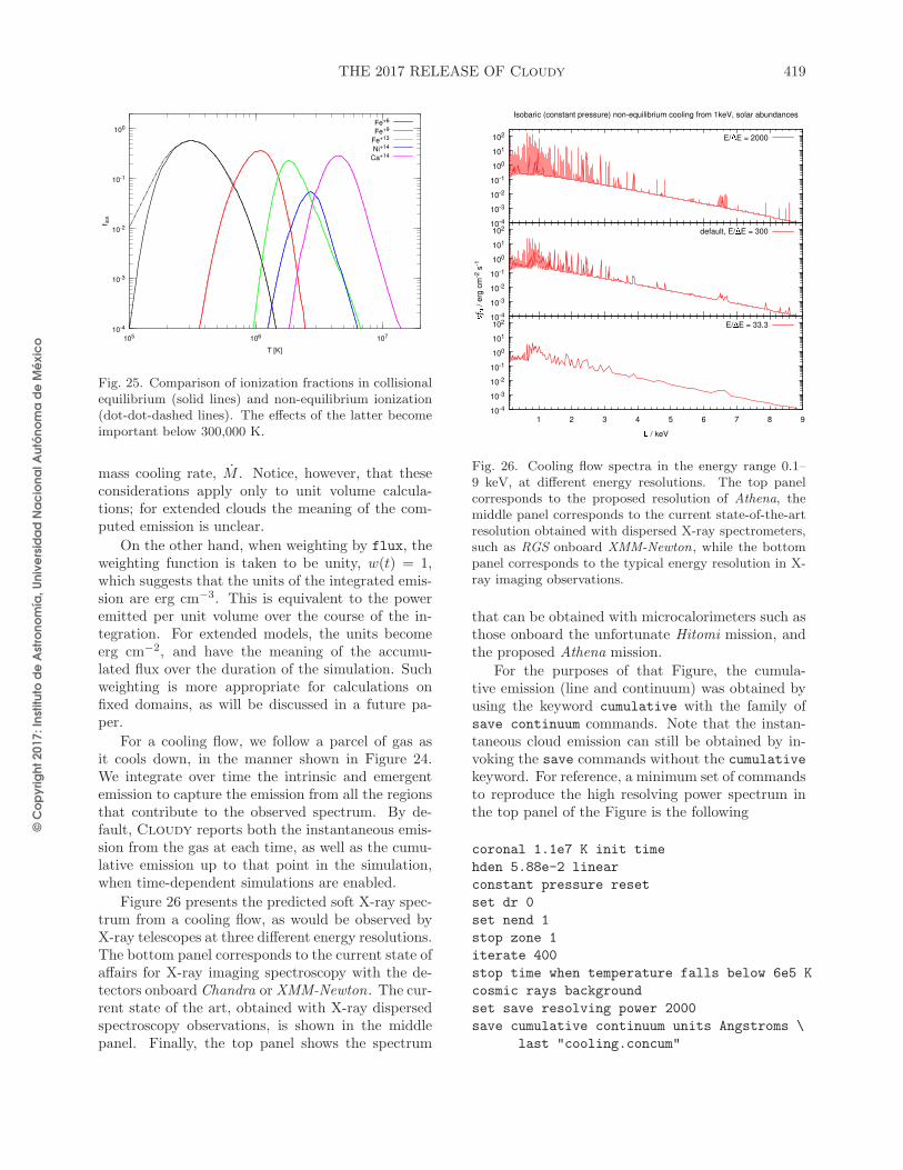
© C
op
yri
gh
t 2
01
7: In
stitu
to d
e A
stro
no
mía
, U
niv
ers
ida
d N
ac
ion
al A
utó
no
ma
de
Mé
xic
o
THE 2017 RELEASE OF Cloudy 419
10-4
10-3
10-2
10-1
100
105 106 107
f ion
T [K]
Fe+6
Fe+9
Fe+13
Ni+14
Ca+14
Fig. 25. Comparison of ionization fractions in collisionalequilibrium (solid lines) and non-equilibrium ionization(dot-dot-dashed lines). The effects of the latter becomeimportant below 300,000 K.
mass cooling rate, M . Notice, however, that theseconsiderations apply only to unit volume calcula-tions; for extended clouds the meaning of the com-puted emission is unclear.
On the other hand, when weighting by flux, theweighting function is taken to be unity, w(t) = 1,which suggests that the units of the integrated emis-sion are erg cm−3. This is equivalent to the poweremitted per unit volume over the course of the in-tegration. For extended models, the units becomeerg cm−2, and have the meaning of the accumu-lated flux over the duration of the simulation. Suchweighting is more appropriate for calculations onfixed domains, as will be discussed in a future pa-per.
For a cooling flow, we follow a parcel of gas asit cools down, in the manner shown in Figure 24.We integrate over time the intrinsic and emergentemission to capture the emission from all the regionsthat contribute to the observed spectrum. By de-fault, Cloudy reports both the instantaneous emis-sion from the gas at each time, as well as the cumu-lative emission up to that point in the simulation,when time-dependent simulations are enabled.
Figure 26 presents the predicted soft X-ray spec-trum from a cooling flow, as would be observed byX-ray telescopes at three different energy resolutions.The bottom panel corresponds to the current state ofaffairs for X-ray imaging spectroscopy with the de-tectors onboard Chandra or XMM-Newton. The cur-rent state of the art, obtained with X-ray dispersedspectroscopy observations, is shown in the middlepanel. Finally, the top panel shows the spectrum
10-4
10-3
10-2
10-1
100
101
102
Isobaric (constant pressure) non-equilibrium cooling from 1keV, solar abundances
E/�E = 2000
10-4
10-3
10-2
10-1
100
101
102 default, E/�E = 300
10-4
10-3
10-2
10-1
100
101
102
1 2 3 4 5 6 7 8 9
✁
ƒ ✂
/ e
rg c
m-2
s-1
✄ / keV
E/�E = 33.3
Fig. 26. Cooling flow spectra in the energy range 0.1–9 keV, at different energy resolutions. The top panelcorresponds to the proposed resolution of Athena, themiddle panel corresponds to the current state-of-the-artresolution obtained with dispersed X-ray spectrometers,such as RGS onboard XMM-Newton, while the bottompanel corresponds to the typical energy resolution in X-ray imaging observations.
that can be obtained with microcalorimeters such asthose onboard the unfortunate Hitomi mission, andthe proposed Athena mission.
For the purposes of that Figure, the cumula-tive emission (line and continuum) was obtained byusing the keyword cumulative with the family ofsave continuum commands. Note that the instan-taneous cloud emission can still be obtained by in-voking the save commands without the cumulativekeyword. For reference, a minimum set of commandsto reproduce the high resolving power spectrum inthe top panel of the Figure is the following
coronal 1.1e7 K init time
hden 5.88e-2 linear
constant pressure reset
set dr 0
set nend 1
stop zone 1
iterate 400
stop time when temperature falls below 6e5 K
cosmic rays background
set save resolving power 2000
save cumulative continuum units Angstroms \
last "cooling.concum"
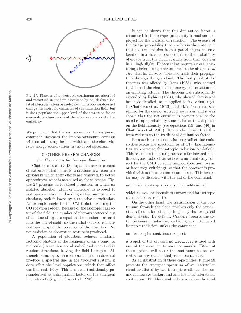
© C
op
yri
gh
t 2
01
7: In
stitu
to d
e A
stro
no
mía
, U
niv
ers
ida
d N
ac
ion
al A
utó
no
ma
de
Mé
xic
o
420 FERLAND ET AL.
Fig. 27. Photons of an isotropic continuum are absorbedand reemitted in random directions by an idealized iso-lated absorber (atom or molecule). This process does notchange the isotropic character of the radiation field, butit does populate the upper level of the transition for anensemble of absorbers, and therefore moderates the lineemissivity.
We point out that the set save resolving power
command increases the line-to-continuum contrastwithout adjusting the line width and therefore vio-lates energy conservation in the saved spectrum.
7. OTHER PHYSICS CHANGES
7.1. Corrections for Isotropic Radiation
Chatzikos et al. (2013) expanded our treatmentof isotropic radiation fields to produce new reportingoptions in which their effects are removed, to betterapproximate what is measured at the telescope. Fig-ure 27 presents an idealized situation, in which anisolated absorber (atom or molecule) is exposed toisotropic radiation, and undergoes two successive ex-citations, each followed by a radiative deexcitation.An example might be the CMB photo-exciting theCO rotation ladder. Because of the isotropic charac-ter of the field, the number of photons scattered outof the line of sight is equal to the number scatteredinto the line-of-sight, so the radiation field remainsisotropic despite the presence of the absorber. Nonet emission or absorption feature is produced.
A population of absorbers behaves similarly.Isotropic photons at the frequency of an atomic (ormolecular) transition are absorbed and reemitted inrandom directions, leaving the field isotropic. Al-though pumping by an isotropic continuum does notproduce a spectral line in the two-level system, itdoes affect the level populations, which then affectthe line emissivity. This has been traditionally pa-rameterized as a diminution factor on the emergentline intensity (e.g., D’Cruz et al. 1998).
It can be shown that this diminution factor isconnected to the escape probability formalism em-ployed for the transfer of radiation. The essence ofthe escape probability theorem lies in the statementthat the net emission from a parcel of gas at somelocation in a cloud is proportional to the probabilityof escape from the cloud starting from that locationin a single flight. Photons that require several scat-terings before escape are assumed to be absorbed insitu, that is, Cloudy does not track their propaga-tion through the gas cloud. The first proof of thetheorem was offered by Irons (1978), who showedthat it had the character of energy conservation foran emitting volume. The theorem was subsequentlyextended by Rybicki (1984), who showed that it wasfar more detailed, as it applied to individual rays.In Chatzikos et al. (2013), Rybicki’s formalism wasrefined for the case of isotropic radiation, and it wasshown that the net emission is proportional to theusual escape probability times a factor that dependson the field intensity (see equations (39) and (40) inChatzikos et al. 2013). It was also shown that thisform reduces to the traditional diminution factor.
Because isotropic radiation may affect line emis-sivities across the spectrum, as of C17, line intensi-ties are corrected for isotropic radiation by default.This resembles the usual practice in far infrared, mil-limeter, and radio observations to automatically cor-rect for the CMB by some method (position, beam,or frequency switching), so that the observer is pro-vided with net line or continuum fluxes. This behav-ior may be disabled with the aid of the command:
no lines isotropic continuum subtraction
which causes line intensities uncorrected for isotropicradiation to be reported.
On the other hand, the transmission of the con-tinuum through the cloud involves only the attenu-ation of radiation at some frequency due to opticaldepth effects. By default, Cloudy reports the to-tal continuum radiation, including any attenuatedisotropic radiation, unless the command:
no isotropic continuua report
is issued, or the keyword no isotropic is used withany of the save continuum commands. Either ofthese options will cause the continuum to be cor-rected for any (attenuated) isotropic radiation.
As an illustration of these capabilities, Figure 28presents the emergent spectrum of an interstellarcloud irradiated by two isotropic continua: the cos-mic microwave background and the local interstellarcontinuum. The black and red curves show the total
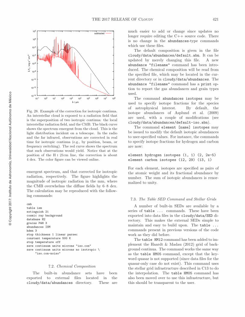
© C
op
yri
gh
t 2
01
7: In
stitu
to d
e A
stro
no
mía
, U
niv
ers
ida
d N
ac
ion
al A
utó
no
ma
de
Mé
xic
o
THE 2017 RELEASE OF Cloudy 421
10-14
10-12
10-10
10-8
10-6
10-4
10-2
100
102
10-1 100 101 102 103 104 105 106 107 108
�
F
✁
/ e
rg s
-1 c
m-2
✂ / µm
subtracted
Fig. 28. Example of the correction for isotropic continua.An interstellar cloud is exposed to a radiation field thatis the superposition of two isotropic continua: the localinterstellar radiation field, and the CMB. The black curveshows the spectrum emergent from the cloud. This is thelight distribution incident on a telescope. In the radioand the far infrared, observations are corrected in realtime for isotropic continua (e.g., by position, beam, orfrequency switching). The red curve shows the spectrumthat such observations would yield. Notice that at theposition of the H i 21cm line, the correction is about4 dex. The color figure can be viewed online.
emergent spectrum, and that corrected for isotropicradiation, respectively. The figure highlights themagnitude of isotropic radiation in the mm, wherethe CMB overwhelms the diffuse fields by 6–8 dex.The calculation may be reproduced with the follow-ing commands:
cmb
table ism
extinguish 21
cosmic ray background
database H2
grains PAH 3
abundances ISM
hden 3
stop thickness 1 linear parsec
constant temperature 500 K
stop temperature off
save continuum units microns "iso.con"
save continuum units microns no isotropic \
"iso.con-noiso"
7.2. Chemical Composition
The built-in abundance sets have beenexported to external files located in thecloudy/data/abundances directory. These are
much easier to add or change since updates nolonger require editing the C++ source code. Thereis no change in the abundances-type commandswhich use these files.
The default composition is given in the filecloudy/data/abundances/default.abn. It can beupdated by merely changing this file. A newabundance "filename" command has been intro-duced. The chemical composition will be read fromthe specified file, which may be located in the cur-rent directory or in cloudy/data/abundances. Theabundance "filename" command has a print op-tion to report the gas abundances and grain typesused.
The command abundances isotopes may beused to specify isotope fractions for the speciesof astrophysical interest. By default, theisotope abundances of Asplund et al. (2009)are used, with a couple of modifications (seecloudy/data/abundances/default-iso.abn).
The command element [name] isotopes maybe issued to modify the default isotopic abundancesto user-specified values. For instance, the commandsto specify isotope fractions for hydrogen and carbonare now:
element hydrogen isotopes (1, 1) (2, 2e-5)
element carbon isotopes (12, 29) (13, 1)
For each element, isotopes are specified as pairs ofthe atomic weight and its fractional abundance bynumber. The sum of isotopic abundances is renor-malized to unity.
7.3. The Table SED Command and Stellar Grids
A number of built-in SEDs are available by aseries of table ... commands. These have beenexported into data files in the cloudy/data/SED di-rectory. This makes the external SEDs simple tomaintain and easy to build upon. The table ...
commands present in previous versions of the codework as they did before.
The table HM12 command has been added to im-plement the Haardt & Madau (2012) grid of back-ground continua. The command works the same wayas the table HM05 command, except that the key-word quasar is not supported (since data files for thequasar-only case do not exist). This command usesthe stellar grid infrastructure described in C13 to dothe interpolation. The table HM05 command hasalso been moved over to use this infrastructure, butthis should be transparent to the user.
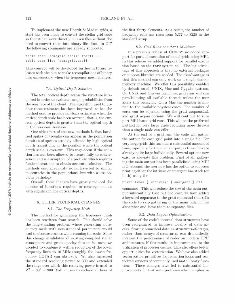
© C
op
yri
gh
t 2
01
7: In
stitu
to d
e A
stro
no
mía
, U
niv
ers
ida
d N
ac
ion
al A
utó
no
ma
de
Mé
xic
o
422 FERLAND ET AL.
To implement the new Haardt & Madau grids, astart has been made to convert the stellar grid codeso that it can work directly on ascii files without theneed to convert them into binary files first. In C17the following commands are already supported.
table star "somegrid.ascii" <par1> ...
table star list "somegrid.ascii"
This concept will be developed further in future re-leases with the aim to make recompilations of binaryfiles unnecessary when the frequency mesh changes.
7.4. Optical Depth Solution
The total optical depth across the structure is re-quired in order to evaluate escape probabilities fromthe rear face of the cloud. The algorithm used to up-date these estimates has been improved, as has themethod used to provide fall-back estimates when theoptical depth scale has been overrun, that is, the cur-rent optical depth is greater than the optical depthin the previous iteration.
One side-effect of the new methods is that local-ized spikes or troughs can appear in the populationdensities of species strongly affected by high opticaldepth transitions, at the position where the opticaldepth scale is over-run. This may occur if the solu-tion has not been allowed to iterate fully to conver-gence, and is a symptom of a problem which requiresfurther iterations to obtain accurate solutions. Themethods used previously would have led to similarinaccuracies in the populations, but with a less ob-vious pathology.
Overall, these changes have greatly reduced thenumber of iterations required to converge modelswith significant line optical depths.
8. OTHER TECHNICAL CHANGES
8.1. The Frequency Mesh
The method for generating the frequency meshhas been rewritten from scratch. This should solvethe long-standing problem where generating a fre-quency mesh with non-standard parameters wouldlead to obscure crashes while running the code. Sincethis change invalidates all existing compiled stellaratmosphere and grain opacity files on its own, wedecided to combine it with a reduction of the lowerfrequency limit to 10 MHz (roughly the lowest fre-quency LOFAR can observe). We also increasedthe standard resolving power to 300 and extendedthe range over which this resolving power is used toZ2 = 302 = 900 Ryd, chosen to include all lines of
the first thirty elements. As a result, the number offrequency cells has risen from 5277 to 8228 in thestandard setup.
8.2. Grid Runs now fork Multicore
In a previous release of Cloudy we added sup-port for parallel execution of model grids using MPI.In this release we added support for parallel execu-tion based on the fork system call. The big advan-tage of this approach is that no external packagesor support libraries are needed. The disadvantage isthat this method can only work on a single shared-memory machine. We offer this possibility enabledby default on all UNIX, Mac and Cygwin systems.On UNIX and Cygwin machines, grid runs will runparallel using all available threads unless the useralters this behavior. On a Mac the number is lim-ited to the available physical cores. The number ofcores can be adjusted using the grid sequential
and grid ncpus options. We will continue to sup-port MPI-based grid runs. This will be the preferredmethod for very large grids requiring more threadsthan a single node can offer.
At the end of a grid run, the code will gatherthe output for each grid point into a single file. Forvery large grids this can take a substantial amount oftime, especially for the main output, as these files arealready quite large individually. Several options nowexist to alleviate this problem. First of all, gather-ing the main output has been parallelized using MPII/O. Second, the user now has the option to suppressprinting either the intrinsic or emergent line stack (orboth) using the
print lines [ intrinsic | emergent ] off
command. This will reduce the size of the main out-put substantially Last but not least, we have addeda keyword separate to the grid command that tellsthe code to skip gathering of the main output filesaltogether and leave them as separate files.
8.3. Data Layout Optimizations
Some of the code’s internal data structures havebeen reorganized to improve locality of data ac-cess. Storing numerical data as structures-of-arrays,rather than arrays-of-structures, can dramaticallyincrease the performance of codes on modern CPUarchitectures, if this results in improvements to theutilization of processor caches. This also offers betteropportunities for vectorization. We have also addedvectorization primitives for reduction loops and vec-torized versions of commonly used math library func-tions. These changes have led to substantial im-provements for test suite problems which emphasize
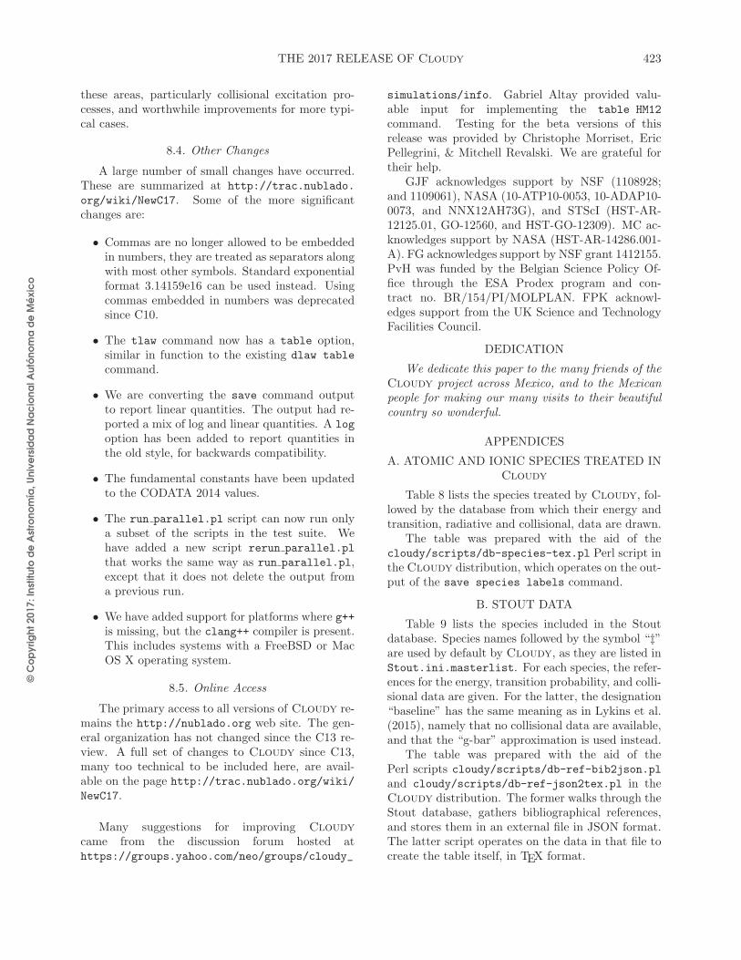
© C
op
yri
gh
t 2
01
7: In
stitu
to d
e A
stro
no
mía
, U
niv
ers
ida
d N
ac
ion
al A
utó
no
ma
de
Mé
xic
o
THE 2017 RELEASE OF Cloudy 423
these areas, particularly collisional excitation pro-cesses, and worthwhile improvements for more typi-cal cases.
8.4. Other Changes
A large number of small changes have occurred.These are summarized at http://trac.nublado.
org/wiki/NewC17. Some of the more significantchanges are:
• Commas are no longer allowed to be embeddedin numbers, they are treated as separators alongwith most other symbols. Standard exponentialformat 3.14159e16 can be used instead. Usingcommas embedded in numbers was deprecatedsince C10.
• The tlaw command now has a table option,similar in function to the existing dlaw table
command.
• We are converting the save command outputto report linear quantities. The output had re-ported a mix of log and linear quantities. A log
option has been added to report quantities inthe old style, for backwards compatibility.
• The fundamental constants have been updatedto the CODATA 2014 values.
• The run parallel.pl script can now run onlya subset of the scripts in the test suite. Wehave added a new script rerun parallel.pl
that works the same way as run parallel.pl,except that it does not delete the output froma previous run.
• We have added support for platforms where g++is missing, but the clang++ compiler is present.This includes systems with a FreeBSD or MacOS X operating system.
8.5. Online Access
The primary access to all versions of Cloudy re-mains the http://nublado.org web site. The gen-eral organization has not changed since the C13 re-view. A full set of changes to Cloudy since C13,many too technical to be included here, are avail-able on the page http://trac.nublado.org/wiki/NewC17.
Many suggestions for improving Cloudy
came from the discussion forum hosted athttps://groups.yahoo.com/neo/groups/cloudy_
simulations/info. Gabriel Altay provided valu-able input for implementing the table HM12
command. Testing for the beta versions of thisrelease was provided by Christophe Morriset, EricPellegrini, & Mitchell Revalski. We are grateful fortheir help.
GJF acknowledges support by NSF (1108928;and 1109061), NASA (10-ATP10-0053, 10-ADAP10-0073, and NNX12AH73G), and STScI (HST-AR-12125.01, GO-12560, and HST-GO-12309). MC ac-knowledges support by NASA (HST-AR-14286.001-A). FG acknowledges support by NSF grant 1412155.PvH was funded by the Belgian Science Policy Of-fice through the ESA Prodex program and con-tract no. BR/154/PI/MOLPLAN. FPK acknowl-edges support from the UK Science and TechnologyFacilities Council.
DEDICATION
We dedicate this paper to the many friends of theCloudy project across Mexico, and to the Mexicanpeople for making our many visits to their beautifulcountry so wonderful.
APPENDICES
A. ATOMIC AND IONIC SPECIES TREATED INCloudy
Table 8 lists the species treated by Cloudy, fol-lowed by the database from which their energy andtransition, radiative and collisional, data are drawn.
The table was prepared with the aid of thecloudy/scripts/db-species-tex.pl Perl script inthe Cloudy distribution, which operates on the out-put of the save species labels command.
B. STOUT DATA
Table 9 lists the species included in the Stoutdatabase. Species names followed by the symbol “‡”are used by default by Cloudy, as they are listed inStout.ini.masterlist. For each species, the refer-ences for the energy, transition probability, and colli-sional data are given. For the latter, the designation“baseline” has the same meaning as in Lykins et al.(2015), namely that no collisional data are available,and that the “g-bar” approximation is used instead.
The table was prepared with the aid of thePerl scripts cloudy/scripts/db-ref-bib2json.pland cloudy/scripts/db-ref-json2tex.pl in theCloudy distribution. The former walks through theStout database, gathers bibliographical references,and stores them in an external file in JSON format.The latter script operates on the data in that file tocreate the table itself, in TEX format.
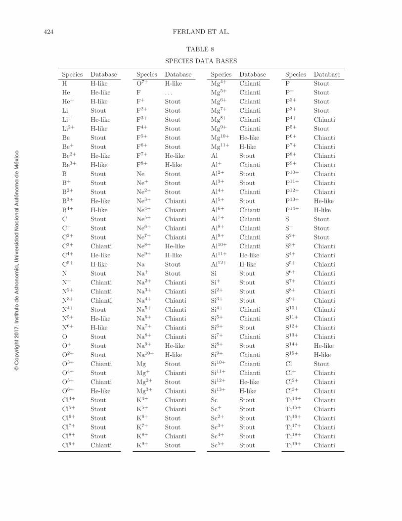
© C
op
yri
gh
t 2
01
7: In
stitu
to d
e A
stro
no
mía
, U
niv
ers
ida
d N
ac
ion
al A
utó
no
ma
de
Mé
xic
o
424 FERLAND ET AL.
TABLE 8
SPECIES DATA BASES
Species Database Species Database Species Database Species Database
H H-like O7+ H-like Mg4+ Chianti P Stout
He He-like F . . . Mg5+ Chianti P+ Stout
He+ H-like F+ Stout Mg6+ Chianti P2+ Stout
Li Stout F2+ Stout Mg7+ Chianti P3+ Stout
Li+ He-like F3+ Stout Mg8+ Chianti P4+ Chianti
Li2+ H-like F4+ Stout Mg9+ Chianti P5+ Stout
Be Stout F5+ Stout Mg10+ He-like P6+ Chianti
Be+ Stout F6+ Stout Mg11+ H-like P7+ Chianti
Be2+ He-like F7+ He-like Al Stout P8+ Chianti
Be3+ H-like F8+ H-like Al+ Chianti P9+ Chianti
B Stout Ne Stout Al2+ Stout P10+ Chianti
B+ Stout Ne+ Stout Al3+ Stout P11+ Chianti
B2+ Stout Ne2+ Stout Al4+ Chianti P12+ Chianti
B3+ He-like Ne3+ Chianti Al5+ Stout P13+ He-like
B4+ H-like Ne4+ Chianti Al6+ Chianti P14+ H-like
C Stout Ne5+ Chianti Al7+ Chianti S Stout
C+ Stout Ne6+ Chianti Al8+ Chianti S+ Stout
C2+ Stout Ne7+ Chianti Al9+ Chianti S2+ Stout
C3+ Chianti Ne8+ He-like Al10+ Chianti S3+ Chianti
C4+ He-like Ne9+ H-like Al11+ He-like S4+ Chianti
C5+ H-like Na Stout Al12+ H-like S5+ Chianti
N Stout Na+ Stout Si Stout S6+ Chianti
N+ Chianti Na2+ Chianti Si+ Stout S7+ Chianti
N2+ Chianti Na3+ Chianti Si2+ Stout S8+ Chianti
N3+ Chianti Na4+ Chianti Si3+ Stout S9+ Chianti
N4+ Stout Na5+ Chianti Si4+ Chianti S10+ Chianti
N5+ He-like Na6+ Chianti Si5+ Chianti S11+ Chianti
N6+ H-like Na7+ Chianti Si6+ Stout S12+ Chianti
O Stout Na8+ Chianti Si7+ Chianti S13+ Chianti
O+ Stout Na9+ He-like Si8+ Stout S14+ He-like
O2+ Stout Na10+ H-like Si9+ Chianti S15+ H-like
O3+ Chianti Mg Stout Si10+ Chianti Cl Stout
O4+ Stout Mg+ Chianti Si11+ Chianti Cl+ Chianti
O5+ Chianti Mg2+ Stout Si12+ He-like Cl2+ Chianti
O6+ He-like Mg3+ Chianti Si13+ H-like Cl3+ Chianti
Cl4+ Stout K4+ Chianti Sc Stout Ti14+ Chianti
Cl5+ Stout K5+ Chianti Sc+ Stout Ti15+ Chianti
Cl6+ Stout K6+ Stout Sc2+ Stout Ti16+ Chianti
Cl7+ Stout K7+ Stout Sc3+ Stout Ti17+ Chianti
Cl8+ Stout K8+ Chianti Sc4+ Stout Ti18+ Chianti
Cl9+ Chianti K9+ Stout Sc5+ Stout Ti19+ Chianti

© C
op
yri
gh
t 2
01
7: In
stitu
to d
e A
stro
no
mía
, U
niv
ers
ida
d N
ac
ion
al A
utó
no
ma
de
Mé
xic
o
THE 2017 RELEASE OF Cloudy 425
TABLE 8 (CONTINUED)
Species Database Species Database Species Database Species Database
Cl10+ Chianti K10+ Chianti Sc6+ Stout Ti20+ He-like
Cl11+ Chianti K11+ Chianti Sc7+ Stout Ti21+ H-like
Cl12+ . . . K12+ Chianti Sc8+ Stout V . . .
Cl13+ Chianti K13+ Chianti Sc9+ Stout V+ . . .
Cl14+ . . . K14+ Chianti Sc10+ Stout V2+ . . .
Cl15+ He-like K15+ Chianti Sc11+ Stout V3+ Stout
Cl16+ H-like K16+ Chianti Sc12+ Stout V4+ . . .
Ar Stout K17+ He-like Sc13+ Stout V5+ Stout
Ar+ Stout K18+ H-like Sc14+ Stout V6+ Stout
Ar2+ Stout Ca Stout Sc15+ Stout V7+ Stout
Ar3+ Stout Ca+ Chianti Sc16+ Stout V8+ Stout
Ar4+ Stout Ca2+ Stout Sc17+ Stout V9+ Stout
Ar5+ Stout Ca3+ Stout Sc18+ . . . V10+ Stout
Ar6+ Chianti Ca4+ Chianti Sc19+ He-like V11+ Stout
Ar7+ Chianti Ca5+ Stout Sc20+ H-like V12+ Stout
Ar8+ Chianti Ca6+ Chianti Ti . . . V13+ . . .
Ar9+ Chianti Ca7+ Chianti Ti+ . . . V14+ Stout
Ar10+ Chianti Ca8+ Chianti Ti2+ Stout V15+ Stout
Ar11+ Chianti Ca9+ Chianti Ti3+ Stout V16+ Stout
Ar12+ Chianti Ca10+ Chianti Ti4+ Stout V17+ Stout
Ar13+ Chianti Ca11+ Chianti Ti5+ Stout V18+ Stout
Ar14+ Chianti Ca12+ Chianti Ti6+ Stout V19+ Stout
Ar15+ Chianti Ca13+ Chianti Ti7+ Stout V20+ Stout
Ar16+ He-like Ca14+ Chianti Ti8+ Stout V21+ He-like
Ar17+ H-like Ca15+ Chianti Ti9+ Stout V22+ H-like
K Stout Ca16+ Chianti Ti10+ Chianti Cr . . .
K+ Stout Ca17+ Chianti Ti11+ Chianti Cr+ Stout
K2+ Stout Ca18+ He-like Ti12+ Stout Cr2+ . . .
K3+ Stout Ca19+ H-like Ti13+ Chianti Cr3+ Stout
Cr4+ Stout Mn15+ Stout Fe25+ H-like Ni6+ Stout
Cr5+ . . . Mn16+ Chianti Co . . . Ni7+ . . .
Cr6+ Chianti Mn17+ Chianti Co+ . . . Ni8+ Stout
Cr7+ Chianti Mn18+ Chianti Co+ Stout Ni9+ . . .
Cr8+ Chianti Mn19+ Chianti Co2+ Stout Ni10+ Stout
Cr9+ Stout Mn20+ Chianti Co3+ . . . Ni11+ Chianti
Cr10+ Stout Mn21+ Chianti Co4+ . . . Ni12+ Chianti
Cr11+ Stout Mn22+ Chianti Co5+ . . . Ni13+ Chianti
Cr12+ Chianti Mn23+ He-like Co6+ . . . Ni14+ Stout
Cr13+ Chianti Mn24+ H-like Co7+ Stout Ni15+ Chianti
Cr14+ Stout Fe Stout Co8+ . . . Ni16+ Chianti
Cr15+ Chianti Fe+ Stout Co9+ Stout Ni17+ Chianti
Cr16+ Chianti Fe2+ Stout Co10+ Stout Ni18+ Chianti
Cr17+ Chianti Fe3+ Chianti Co11+ Stout Ni19+ Chianti
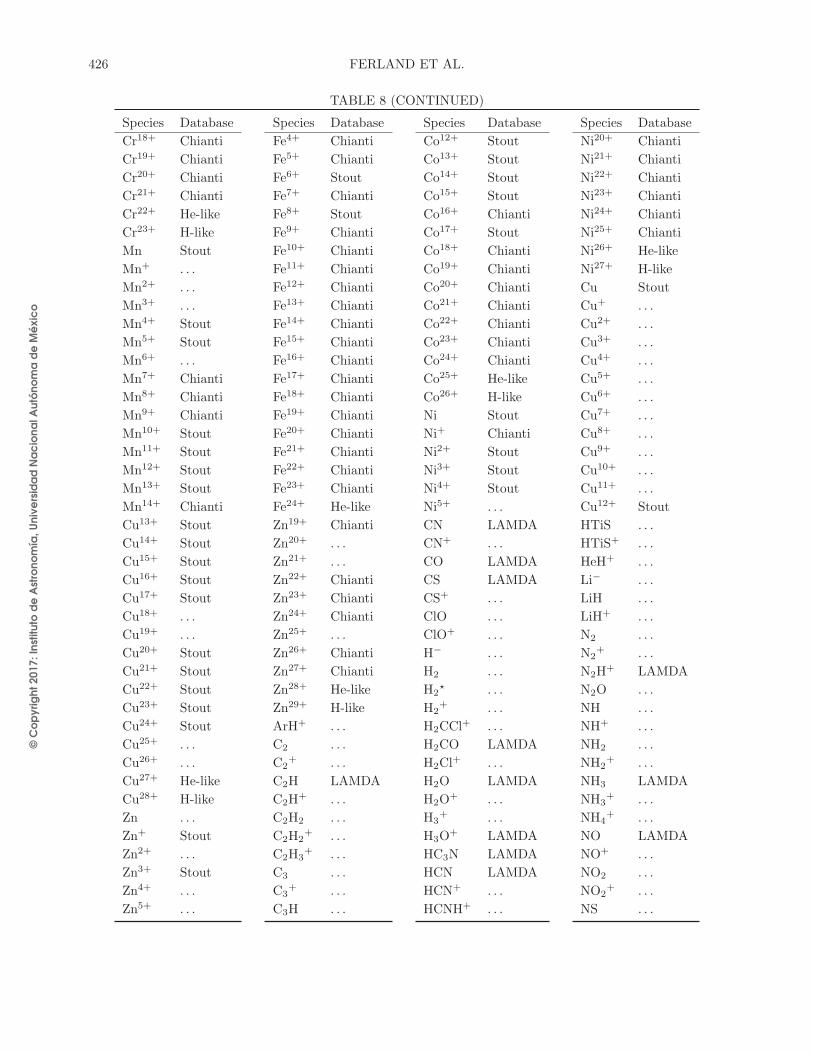
© C
op
yri
gh
t 2
01
7: In
stitu
to d
e A
stro
no
mía
, U
niv
ers
ida
d N
ac
ion
al A
utó
no
ma
de
Mé
xic
o
426 FERLAND ET AL.
TABLE 8 (CONTINUED)
Species Database Species Database Species Database Species Database
Cr18+ Chianti Fe4+ Chianti Co12+ Stout Ni20+ Chianti
Cr19+ Chianti Fe5+ Chianti Co13+ Stout Ni21+ Chianti
Cr20+ Chianti Fe6+ Stout Co14+ Stout Ni22+ Chianti
Cr21+ Chianti Fe7+ Chianti Co15+ Stout Ni23+ Chianti
Cr22+ He-like Fe8+ Stout Co16+ Chianti Ni24+ Chianti
Cr23+ H-like Fe9+ Chianti Co17+ Stout Ni25+ Chianti
Mn Stout Fe10+ Chianti Co18+ Chianti Ni26+ He-like
Mn+ . . . Fe11+ Chianti Co19+ Chianti Ni27+ H-like
Mn2+ . . . Fe12+ Chianti Co20+ Chianti Cu Stout
Mn3+ . . . Fe13+ Chianti Co21+ Chianti Cu+ . . .
Mn4+ Stout Fe14+ Chianti Co22+ Chianti Cu2+ . . .
Mn5+ Stout Fe15+ Chianti Co23+ Chianti Cu3+ . . .
Mn6+ . . . Fe16+ Chianti Co24+ Chianti Cu4+ . . .
Mn7+ Chianti Fe17+ Chianti Co25+ He-like Cu5+ . . .
Mn8+ Chianti Fe18+ Chianti Co26+ H-like Cu6+ . . .
Mn9+ Chianti Fe19+ Chianti Ni Stout Cu7+ . . .
Mn10+ Stout Fe20+ Chianti Ni+ Chianti Cu8+ . . .
Mn11+ Stout Fe21+ Chianti Ni2+ Stout Cu9+ . . .
Mn12+ Stout Fe22+ Chianti Ni3+ Stout Cu10+ . . .
Mn13+ Stout Fe23+ Chianti Ni4+ Stout Cu11+ . . .
Mn14+ Chianti Fe24+ He-like Ni5+ . . . Cu12+ Stout
Cu13+ Stout Zn19+ Chianti CN LAMDA HTiS . . .
Cu14+ Stout Zn20+ . . . CN+ . . . HTiS+ . . .
Cu15+ Stout Zn21+ . . . CO LAMDA HeH+ . . .
Cu16+ Stout Zn22+ Chianti CS LAMDA Li− . . .
Cu17+ Stout Zn23+ Chianti CS+ . . . LiH . . .
Cu18+ . . . Zn24+ Chianti ClO . . . LiH+ . . .
Cu19+ . . . Zn25+ . . . ClO+ . . . N2 . . .
Cu20+ Stout Zn26+ Chianti H− . . . N2+ . . .
Cu21+ Stout Zn27+ Chianti H2 . . . N2H+ LAMDA
Cu22+ Stout Zn28+ He-like H2⋆ . . . N2O . . .
Cu23+ Stout Zn29+ H-like H2+ . . . NH . . .
Cu24+ Stout ArH+ . . . H2CCl+ . . . NH+ . . .
Cu25+ . . . C2 . . . H2CO LAMDA NH2 . . .
Cu26+ . . . C2+ . . . H2Cl
+ . . . NH2+ . . .
Cu27+ He-like C2H LAMDA H2O LAMDA NH3 LAMDA
Cu28+ H-like C2H+ . . . H2O
+ . . . NH3+ . . .
Zn . . . C2H2 . . . H3+ . . . NH4
+ . . .
Zn+ Stout C2H2+ . . . H3O
+ LAMDA NO LAMDA
Zn2+ . . . C2H3+ . . . HC3N LAMDA NO+ . . .
Zn3+ Stout C3 . . . HCN LAMDA NO2 . . .
Zn4+ . . . C3+ . . . HCN+ . . . NO2
+ . . .
Zn5+ . . . C3H . . . HCNH+ . . . NS . . .

© C
op
yri
gh
t 2
01
7: In
stitu
to d
e A
stro
no
mía
, U
niv
ers
ida
d N
ac
ion
al A
utó
no
ma
de
Mé
xic
o
THE 2017 RELEASE OF Cloudy 427
TABLE 8 (CONTINUED)
Species Database Species Database Species Database Species Database
Zn6+ . . . C3H+ . . . HCO+ LAMDA NS+ . . .
Zn7+ . . . CCl . . . HCS+ LAMDA NeH+ . . .
Zn8+ . . . CCl+ . . . HCTi . . . O2 LAMDA
Zn9+ . . . CH . . . HCTi+ . . . O2+ . . .
Zn10+ . . . CH+ . . . HCl LAMDA OCN . . .
Zn11+ . . . CH2 . . . HCl+ . . . OCN+ . . .
Zn12+ . . . CH2+ . . . HNC LAMDA OCS LAMDA
Zn13+ . . . CH3 . . . HNO . . . OCS+ . . .
Zn14+ . . . CH3+ . . . HNO+ . . . OH LAMDA
Zn15+ . . . CH3OH LAMDA HNTi . . . OH+ LAMDA
Zn16+ . . . CH4 . . . HNTi+ . . . S2 . . .
Zn17+ . . . CH4+ . . . HS . . . S2
+ . . .
Zn18+ Stout CH5+ . . . HS+ . . . SO LAMDA
SO+ . . . SiO+ . . . TiH+ . . . TiO+ . . .
SO2 LAMDA SiOH+ . . . TiH2 . . . TiO2 . . .
SiC2 LAMDA TiC . . . TiH2+ . . . TiOH+ . . .
SiH . . . TiC+ . . . TiN . . . TiS . . .
SiH2+ . . . TiC2 . . . TiN+ . . . TiS+ . . .
SiN . . . TiC2+ . . . TiNC . . . 13CO LAMDA
SiN+ . . . TiF+ . . . TiNC+ . . .
SiO LAMDA TiH . . . TiO . . .
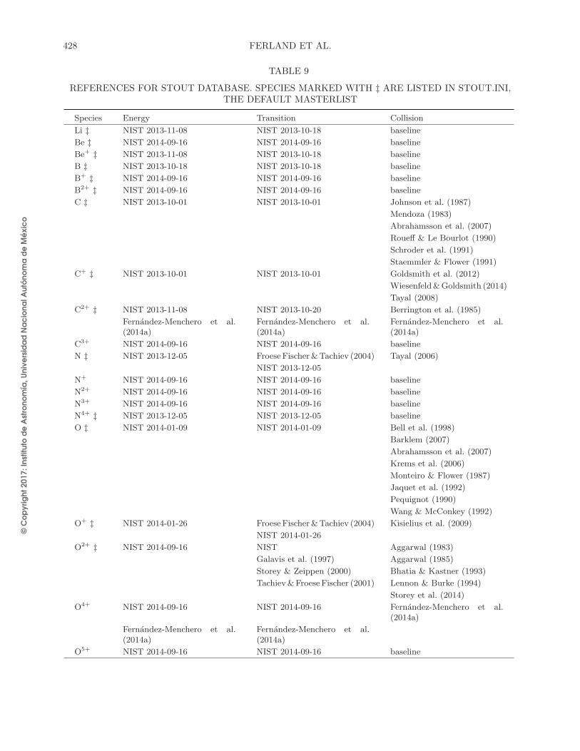
© C
op
yri
gh
t 2
01
7: In
stitu
to d
e A
stro
no
mía
, U
niv
ers
ida
d N
ac
ion
al A
utó
no
ma
de
Mé
xic
o
428 FERLAND ET AL.
TABLE 9
REFERENCES FOR STOUT DATABASE. SPECIES MARKED WITH ‡ ARE LISTED IN STOUT.INI,THE DEFAULT MASTERLIST
Species Energy Transition Collision
Li ‡ NIST 2013-11-08 NIST 2013-10-18 baseline
Be ‡ NIST 2014-09-16 NIST 2014-09-16 baseline
Be+ ‡ NIST 2013-11-08 NIST 2013-10-18 baseline
B ‡ NIST 2013-10-18 NIST 2013-10-18 baseline
B+ ‡ NIST 2014-09-16 NIST 2014-09-16 baseline
B2+ ‡ NIST 2014-09-16 NIST 2014-09-16 baseline
C ‡ NIST 2013-10-01 NIST 2013-10-01 Johnson et al. (1987)
Mendoza (1983)
Abrahamsson et al. (2007)
Roueff & Le Bourlot (1990)
Schroder et al. (1991)
Staemmler & Flower (1991)
C+ ‡ NIST 2013-10-01 NIST 2013-10-01 Goldsmith et al. (2012)
Wiesenfeld&Goldsmith (2014)
Tayal (2008)
C2+ ‡ NIST 2013-11-08 NIST 2013-10-20 Berrington et al. (1985)
Fernandez-Menchero et al.(2014a)
Fernandez-Menchero et al.(2014a)
Fernandez-Menchero et al.(2014a)
C3+ NIST 2014-09-16 NIST 2014-09-16 baseline
N ‡ NIST 2013-12-05 Froese Fischer&Tachiev (2004) Tayal (2006)
NIST 2013-12-05
N+ NIST 2014-09-16 NIST 2014-09-16 baseline
N2+ NIST 2014-09-16 NIST 2014-09-16 baseline
N3+ NIST 2014-09-16 NIST 2014-09-16 baseline
N4+ ‡ NIST 2013-12-05 NIST 2013-12-05 baseline
O ‡ NIST 2014-01-09 NIST 2014-01-09 Bell et al. (1998)
Barklem (2007)
Abrahamsson et al. (2007)
Krems et al. (2006)
Monteiro & Flower (1987)
Jaquet et al. (1992)
Pequignot (1990)
Wang & McConkey (1992)
O+ ‡ NIST 2014-01-26 Froese Fischer&Tachiev (2004) Kisielius et al. (2009)
NIST 2014-01-26
O2+ ‡ NIST 2014-09-16 NIST Aggarwal (1983)
Galavis et al. (1997) Aggarwal (1985)
Storey & Zeippen (2000) Bhatia & Kastner (1993)
Tachiev&Froese Fischer (2001) Lennon & Burke (1994)
Storey et al. (2014)
O4+ NIST 2014-09-16 NIST 2014-09-16 Fernandez-Menchero et al.(2014a)
Fernandez-Menchero et al.(2014a)
Fernandez-Menchero et al.(2014a)
O5+ NIST 2014-09-16 NIST 2014-09-16 baseline

© C
op
yri
gh
t 2
01
7: In
stitu
to d
e A
stro
no
mía
, U
niv
ers
ida
d N
ac
ion
al A
utó
no
ma
de
Mé
xic
o
THE 2017 RELEASE OF Cloudy 429
TABLE 9 (CONTINUED)
Species Energy Transition Collision
F+ ‡ NIST 2013-10-01 NIST 2013-10-01 Butler & Zeippen (1994)
F2+ ‡ NIST 2014-09-16 NIST 2014-09-16 baseline
F3+ ‡ NIST 2013-10-01 NIST 2013-10-01 Lennon & Burke (1994)
F4+ ‡ NIST 2014-09-16 NIST 2014-09-16 baseline
F5+ ‡ NIST 2014-09-16 NIST 2014-09-16 Fernandez-Menchero et al.(2014a)
Fernandez-Menchero et al.(2014a)
Fernandez-Menchero et al.(2014a)
F6+ ‡ NIST 2014-09-16 NIST 2014-09-16 baseline
Ne ‡ NIST 2014-09-16 NIST 2014-09-16 baseline
Ne+ ‡ NIST 2013-10-01 NIST 2013-10-01 Griffin et al. (2001)
Hollenbach & McKee (1989)
Ne2+ ‡ NIST McLaughlin et al. (2011) McLaughlin et al. (2011)
McLaughlin et al. (2011)
Ne3+ NIST 2014-09-16 NIST 2014-09-16 baseline
Ne4+ NIST 2014-09-16 NIST 2014-09-16 baseline
Ne6+ NIST 2014-09-16 NIST 2014-09-16 baseline
Ne7+ NIST 2014-09-16 NIST 2014-09-16 baseline
Na ‡ NIST 2013-10-01 NIST 2013-10-01 Verner, private communication
Na+ ‡ NIST 2014-09-16 NIST 2014-09-16 baseline
Na2+ NIST 2014-09-16 NIST 2014-09-16 baseline
Na3+ NIST 2014-09-16 NIST 2014-09-16 baseline
Na4+ NIST 2014-09-16 NIST 2014-09-16 baseline
Na5+ NIST 2014-09-16 NIST 2014-09-16 baseline
Na6+ NIST 2014-09-16 NIST 2014-09-16 baseline
Na7+ NIST 2014-09-16 NIST 2014-09-16 baseline
Na8+ NIST 2014-09-16 NIST 2014-09-16 baseline
Mg ‡ NIST 2013-10-01 NIST 2013-10-01 Barklem et al. (2012)
Osorio et al. (2015)
Mg+ NIST 2014-09-16 NIST 2014-09-16 baseline
Mg2+ ‡ NIST 2013-10-01 NIST 2013-10-01 Liang & Badnell (2010)
NIST 2013-09-07
Mg3+ NIST 2014-09-16 NIST 2014-09-16 baseline
Mg4+ NIST 2014-09-16 NIST 2014-09-16 baseline
Mg5+ NIST 2014-09-16 NIST 2014-09-16 baseline
Mg6+ NIST 2014-09-16 NIST 2014-09-16 baseline
Mg7+ NIST 2014-09-16 NIST 2014-09-16 baseline
Mg8+ NIST 2014-09-16 NIST 2014-09-16 baseline
Mg9+ NIST 2014-09-16 NIST 2014-09-16 baseline
Al ‡ NIST 2013-10-01 NIST 2013-10-01 baseline
Al+ NIST 2014-09-16 NIST 2014-09-16 baseline
Al2+ ‡ NIST 2013-10-01 NIST 2013-10-01 Dufton & Kingston (1987)
Al3+ ‡ NIST 2014-09-16 NIST 2014-09-16 baseline
Al4+ NIST 2014-09-16 NIST 2014-09-16 baseline
Al5+ ‡ NIST 2014-05-24 NIST 2014-05-24 Butler & Zeippen (1994)
Al6+ NIST 2014-09-16 NIST 2014-09-16 baseline
Al7+ NIST 2014-09-16 NIST 2014-09-16 baseline
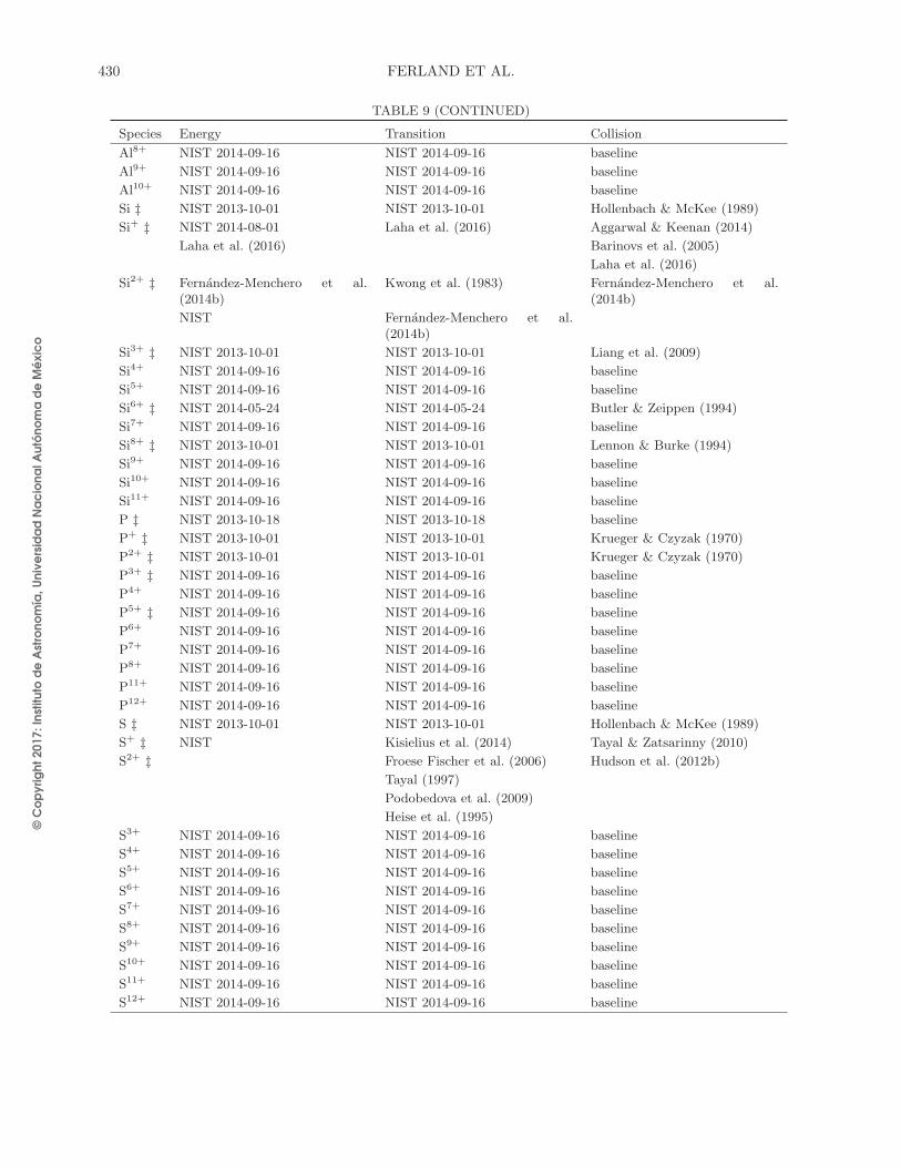
© C
op
yri
gh
t 2
01
7: In
stitu
to d
e A
stro
no
mía
, U
niv
ers
ida
d N
ac
ion
al A
utó
no
ma
de
Mé
xic
o
430 FERLAND ET AL.
TABLE 9 (CONTINUED)
Species Energy Transition Collision
Al8+ NIST 2014-09-16 NIST 2014-09-16 baseline
Al9+ NIST 2014-09-16 NIST 2014-09-16 baseline
Al10+ NIST 2014-09-16 NIST 2014-09-16 baseline
Si ‡ NIST 2013-10-01 NIST 2013-10-01 Hollenbach & McKee (1989)
Si+ ‡ NIST 2014-08-01 Laha et al. (2016) Aggarwal & Keenan (2014)
Laha et al. (2016) Barinovs et al. (2005)
Laha et al. (2016)
Si2+ ‡ Fernandez-Menchero et al.(2014b)
Kwong et al. (1983) Fernandez-Menchero et al.(2014b)
NIST Fernandez-Menchero et al.(2014b)
Si3+ ‡ NIST 2013-10-01 NIST 2013-10-01 Liang et al. (2009)
Si4+ NIST 2014-09-16 NIST 2014-09-16 baseline
Si5+ NIST 2014-09-16 NIST 2014-09-16 baseline
Si6+ ‡ NIST 2014-05-24 NIST 2014-05-24 Butler & Zeippen (1994)
Si7+ NIST 2014-09-16 NIST 2014-09-16 baseline
Si8+ ‡ NIST 2013-10-01 NIST 2013-10-01 Lennon & Burke (1994)
Si9+ NIST 2014-09-16 NIST 2014-09-16 baseline
Si10+ NIST 2014-09-16 NIST 2014-09-16 baseline
Si11+ NIST 2014-09-16 NIST 2014-09-16 baseline
P ‡ NIST 2013-10-18 NIST 2013-10-18 baseline
P+ ‡ NIST 2013-10-01 NIST 2013-10-01 Krueger & Czyzak (1970)
P2+ ‡ NIST 2013-10-01 NIST 2013-10-01 Krueger & Czyzak (1970)
P3+ ‡ NIST 2014-09-16 NIST 2014-09-16 baseline
P4+ NIST 2014-09-16 NIST 2014-09-16 baseline
P5+ ‡ NIST 2014-09-16 NIST 2014-09-16 baseline
P6+ NIST 2014-09-16 NIST 2014-09-16 baseline
P7+ NIST 2014-09-16 NIST 2014-09-16 baseline
P8+ NIST 2014-09-16 NIST 2014-09-16 baseline
P11+ NIST 2014-09-16 NIST 2014-09-16 baseline
P12+ NIST 2014-09-16 NIST 2014-09-16 baseline
S ‡ NIST 2013-10-01 NIST 2013-10-01 Hollenbach & McKee (1989)
S+ ‡ NIST Kisielius et al. (2014) Tayal & Zatsarinny (2010)
S2+ ‡ Froese Fischer et al. (2006) Hudson et al. (2012b)
Tayal (1997)
Podobedova et al. (2009)
Heise et al. (1995)
S3+ NIST 2014-09-16 NIST 2014-09-16 baseline
S4+ NIST 2014-09-16 NIST 2014-09-16 baseline
S5+ NIST 2014-09-16 NIST 2014-09-16 baseline
S6+ NIST 2014-09-16 NIST 2014-09-16 baseline
S7+ NIST 2014-09-16 NIST 2014-09-16 baseline
S8+ NIST 2014-09-16 NIST 2014-09-16 baseline
S9+ NIST 2014-09-16 NIST 2014-09-16 baseline
S10+ NIST 2014-09-16 NIST 2014-09-16 baseline
S11+ NIST 2014-09-16 NIST 2014-09-16 baseline
S12+ NIST 2014-09-16 NIST 2014-09-16 baseline

© C
op
yri
gh
t 2
01
7: In
stitu
to d
e A
stro
no
mía
, U
niv
ers
ida
d N
ac
ion
al A
utó
no
ma
de
Mé
xic
o
THE 2017 RELEASE OF Cloudy 431
TABLE 9 (CONTINUED)
Species Energy Transition Collision
S13+ NIST 2014-09-16 NIST 2014-09-16 baseline
Cl ‡ NIST 2013-10-01 NIST 2013-10-01 Hollenbach & McKee (1989)
Cl+ NIST 2014-09-16 NIST 2014-09-16 baseline
Cl2+ NIST 2014-09-16 NIST 2014-09-16 baseline
Cl3+ NIST 2014-09-16 NIST 2014-09-16 baseline
Cl4+ ‡ NIST 2014-09-16 NIST 2014-09-16 baseline
Cl5+ ‡ NIST Fernandez-Menchero et al.(2014b)
Fernandez-Menchero et al.(2014b)
Fernandez-Menchero et al.(2014b)
Cl6+ ‡ Liang et al. (2009) Liang et al. (2009) Liang et al. (2009)
Cl7+ ‡ Liang & Badnell (2010) Liang & Badnell (2010) Liang & Badnell (2010)
Cl8+ ‡ NIST 2013-10-01 NIST 2013-10-01 Berrington et al. (1998)
Cl9+ NIST 2014-09-16 NIST 2014-09-16 baseline
Ar ‡ NIST 2013-11-08 NIST 2013-10-01 baseline
Ar+ ‡ NIST 2013-10-01 NIST 2013-10-01 Pelan & Berrington (1995)
Ar2+ ‡ NIST 2013-10-01 NIST 2013-10-01 Galavis et al. (1995)
Ar3+ ‡ NIST 2013-10-01 NIST 2013-10-01 Ramsbottom et al. (1997)
Ar4+ ‡ NIST 2013-10-01 NIST 2013-10-01 Galavis et al. (1995)
Ar5+ ‡ NIST 2013-10-01 NIST 2013-10-01 Saraph & Storey (1996)
Ar6+ NIST 2014-09-16 NIST 2014-09-16 baseline
Ar7+ NIST 2014-09-16 NIST 2014-09-16 baseline
Ar8+ NIST 2014-09-16 NIST 2014-09-16 baseline
Ar9+ NIST 2014-09-16 NIST 2014-09-16 baseline
Ar10+ NIST 2014-09-16 NIST 2014-09-16 baseline
Ar12+ NIST 2014-09-16 NIST 2014-09-16 baseline
Ar13+ NIST 2014-09-16 NIST 2014-09-16 baseline
K ‡ NIST 2013-10-01 NIST 2013-10-01 baseline
K+ ‡ NIST 2014-09-16 NIST 2014-09-16 baseline
K2+ ‡ NIST 2013-10-01 NIST 2013-10-01 Pelan & Berrington (1995)
K3+ ‡ NIST 2013-10-01 NIST 2013-10-01 Galavis et al. (1995)
K4+ NIST 2014-09-16 NIST 2014-09-16 baseline
K5+ NIST 2014-09-16 NIST 2014-09-16 baseline
K6+ ‡ NIST 2013-10-01 NIST 2013-10-01 Saraph & Storey (1996)
K7+ ‡ NIST Fernandez-Menchero et al.(2014b)
Fernandez-Menchero et al.(2014b)
Fernandez-Menchero et al.(2014b)
K8+ NIST 2014-09-16 NIST 2014-09-16 baseline
K9+ ‡ NIST 2014-09-16 NIST 2014-09-16 baseline
K10+ NIST 2014-09-16 NIST 2014-09-16 baseline
K11+ NIST 2014-09-16 NIST 2014-09-16 baseline
K12+ NIST 2014-09-16 NIST 2014-09-16 baseline
K13+ NIST 2014-09-16 NIST 2014-09-16 baseline
K14+ NIST 2014-09-16 NIST 2014-09-16 baseline
K15+ NIST 2014-09-16 NIST 2014-09-16 baseline
K16+ NIST 2014-09-16 NIST 2014-09-16 baseline

© C
op
yri
gh
t 2
01
7: In
stitu
to d
e A
stro
no
mía
, U
niv
ers
ida
d N
ac
ion
al A
utó
no
ma
de
Mé
xic
o
432 FERLAND ET AL.
TABLE 9 (CONTINUED)
Species Energy Transition Collision
Ca ‡ NIST 2013-10-01 NIST 2013-10-01 baseline
Ca+ NIST 2014-09-16 NIST 2014-09-16 baseline
Ca2+ ‡ NIST 2014-09-16 NIST 2014-09-16 baseline
Ca3+ ‡ NIST 2013-10-01 NIST 2013-10-01 Pelan & Berrington (1995)
Ca4+ NIST 2014-09-16 NIST 2014-09-16 baseline
Ca5+ ‡ NIST 2014-09-16 NIST 2014-09-16 baseline
Ca6+ NIST 2014-09-16 NIST 2014-09-16 baseline
Ca7+ NIST 2014-09-16 NIST 2014-09-16 baseline
Ca9+ NIST 2014-09-16 NIST 2014-09-16 baseline
Ca10+ NIST 2014-09-16 NIST 2014-09-16 baseline
Ca11+ NIST 2014-09-16 NIST 2014-09-16 baseline
Ca12+ NIST 2014-09-16 NIST 2014-09-16 baseline
Ca14+ NIST 2014-09-16 NIST 2014-09-16 baseline
Sc ‡ NIST 2013-10-18 NIST 2013-10-18 baseline
Sc+ ‡ NIST 2013-10-01 NIST 2013-10-01 Wasson et al. (2011)
Sc2+ ‡ NIST 2013-10-01 NIST 2013-10-01 baseline
Sc3+ ‡ NIST 2014-09-16 NIST 2014-09-16 baseline
Sc4+ ‡ NIST 2013-10-01 NIST 2013-10-01 Pelan & Berrington (1995)
Sc5+ ‡ NIST 2013-10-01 NIST 2013-10-01 baseline
Sc6+ ‡ NIST 2014-09-16 NIST 2014-09-16 baseline
Sc7+ ‡ NIST 2014-09-16 NIST 2014-09-16 baseline
Sc8+ ‡ NIST 2014-09-16 NIST 2014-09-16 baseline
V10+ ‡ NIST 2014-09-16 NIST 2014-09-16 baseline
V11+ ‡ NIST Fernandez-Menchero et al.(2014b)
Fernandez-Menchero et al.(2014b)
V12+ ‡ NIST 2014-09-16 NIST 2014-09-16 baseline
V14+ ‡ NIST NIST Berrington et al. (1998)
NIST NIST
V15+ ‡ NIST 2014-09-16 NIST 2014-09-16 baseline
V16+ ‡ NIST 2014-09-16 NIST 2014-09-16 baseline
V17+ ‡ NIST 2014-09-16 NIST 2014-09-16 baseline
V18+ ‡ NIST 2014-09-16 NIST 2014-09-16 baseline
V19+ ‡ NIST 2014-09-16 NIST 2014-09-16 baseline
V20+ ‡ NIST 2014-09-16 NIST 2014-09-16 baseline
Cr+ ‡ NIST 2013-10-01 NIST 2013-10-01 Grieve & Ramsbottom (2012)
Cr3+ ‡ NIST 2013-10-01 NIST 2013-10-01 baseline
Cr4+ ‡ NIST 2013-10-01 NIST 2013-10-01 baseline
Cr6+ NIST 2014-09-16 NIST 2014-09-16 baseline
Cr8+ NIST 2014-09-16 NIST 2014-09-16 baseline
Cr9+ ‡ NIST 2014-09-16 NIST 2014-09-16 baseline
Cr10+ ‡ NIST 2014-09-16 NIST 2014-09-16 baseline
Cr11+ ‡ NIST 2014-09-16 NIST 2014-09-16 baseline
Cr12+ NIST 2014-09-16 NIST 2014-09-16 baseline
Cr13+ NIST 2014-09-16 NIST 2014-09-16 baseline
Cr14+ ‡ NIST 2014-09-16 NIST 2014-09-16 baseline
Cr15+ NIST 2014-09-16 NIST 2014-09-16 baseline
Cr16+ NIST 2014-09-16 NIST 2014-09-16 baseline
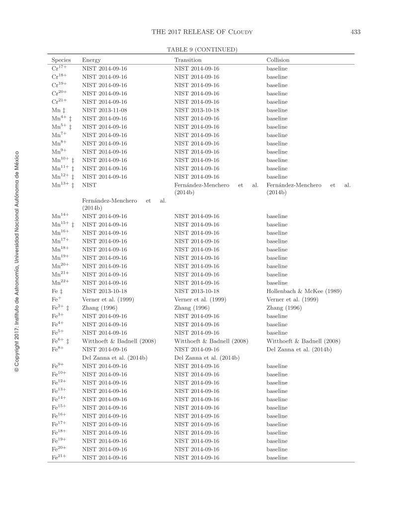
© C
op
yri
gh
t 2
01
7: In
stitu
to d
e A
stro
no
mía
, U
niv
ers
ida
d N
ac
ion
al A
utó
no
ma
de
Mé
xic
o
THE 2017 RELEASE OF Cloudy 433
TABLE 9 (CONTINUED)
Species Energy Transition Collision
Cr17+ NIST 2014-09-16 NIST 2014-09-16 baseline
Cr18+ NIST 2014-09-16 NIST 2014-09-16 baseline
Cr19+ NIST 2014-09-16 NIST 2014-09-16 baseline
Cr20+ NIST 2014-09-16 NIST 2014-09-16 baseline
Cr21+ NIST 2014-09-16 NIST 2014-09-16 baseline
Mn ‡ NIST 2013-11-08 NIST 2013-10-18 baseline
Mn4+ ‡ NIST 2014-09-16 NIST 2014-09-16 baseline
Mn5+ ‡ NIST 2014-09-16 NIST 2014-09-16 baseline
Mn7+ NIST 2014-09-16 NIST 2014-09-16 baseline
Mn8+ NIST 2014-09-16 NIST 2014-09-16 baseline
Mn9+ NIST 2014-09-16 NIST 2014-09-16 baseline
Mn10+ ‡ NIST 2014-09-16 NIST 2014-09-16 baseline
Mn11+ ‡ NIST 2014-09-16 NIST 2014-09-16 baseline
Mn12+ ‡ NIST 2014-09-16 NIST 2014-09-16 baseline
Mn13+ ‡ NIST Fernandez-Menchero et al.(2014b)
Fernandez-Menchero et al.(2014b)
Fernandez-Menchero et al.(2014b)
Mn14+ NIST 2014-09-16 NIST 2014-09-16 baseline
Mn15+ ‡ NIST 2014-09-16 NIST 2014-09-16 baseline
Mn16+ NIST 2014-09-16 NIST 2014-09-16 baseline
Mn17+ NIST 2014-09-16 NIST 2014-09-16 baseline
Mn18+ NIST 2014-09-16 NIST 2014-09-16 baseline
Mn19+ NIST 2014-09-16 NIST 2014-09-16 baseline
Mn20+ NIST 2014-09-16 NIST 2014-09-16 baseline
Mn21+ NIST 2014-09-16 NIST 2014-09-16 baseline
Mn22+ NIST 2014-09-16 NIST 2014-09-16 baseline
Fe ‡ NIST 2013-10-18 NIST 2013-10-18 Hollenbach & McKee (1989)
Fe+ Verner et al. (1999) Verner et al. (1999) Verner et al. (1999)
Fe2+ ‡ Zhang (1996) Zhang (1996) Zhang (1996)
Fe3+ NIST 2014-09-16 NIST 2014-09-16 baseline
Fe4+ NIST 2014-09-16 NIST 2014-09-16 baseline
Fe5+ NIST 2014-09-16 NIST 2014-09-16 baseline
Fe6+ ‡ Witthoeft & Badnell (2008) Witthoeft & Badnell (2008) Witthoeft & Badnell (2008)
Fe8+ NIST 2014-09-16 NIST 2014-09-16 Del Zanna et al. (2014b)
Del Zanna et al. (2014b) Del Zanna et al. (2014b)
Fe9+ NIST 2014-09-16 NIST 2014-09-16 baseline
Fe10+ NIST 2014-09-16 NIST 2014-09-16 baseline
Fe12+ NIST 2014-09-16 NIST 2014-09-16 baseline
Fe13+ NIST 2014-09-16 NIST 2014-09-16 baseline
Fe14+ NIST 2014-09-16 NIST 2014-09-16 baseline
Fe15+ NIST 2014-09-16 NIST 2014-09-16 baseline
Fe16+ NIST 2014-09-16 NIST 2014-09-16 baseline
Fe17+ NIST 2014-09-16 NIST 2014-09-16 baseline
Fe18+ NIST 2014-09-16 NIST 2014-09-16 baseline
Fe19+ NIST 2014-09-16 NIST 2014-09-16 baseline
Fe20+ NIST 2014-09-16 NIST 2014-09-16 baseline
Fe21+ NIST 2014-09-16 NIST 2014-09-16 baseline
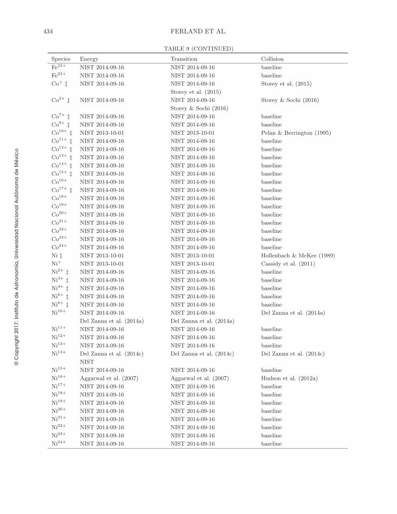
© C
op
yri
gh
t 2
01
7: In
stitu
to d
e A
stro
no
mía
, U
niv
ers
ida
d N
ac
ion
al A
utó
no
ma
de
Mé
xic
o
434 FERLAND ET AL.
TABLE 9 (CONTINUED)
Species Energy Transition Collision
Fe22+ NIST 2014-09-16 NIST 2014-09-16 baseline
Fe23+ NIST 2014-09-16 NIST 2014-09-16 baseline
Co+ ‡ NIST 2014-09-16 NIST 2014-09-16 Storey et al. (2015)
Storey et al. (2015)
Co2+ ‡ NIST 2014-09-16 NIST 2014-09-16 Storey & Sochi (2016)
Storey & Sochi (2016)
Co7+ ‡ NIST 2014-09-16 NIST 2014-09-16 baseline
Co9+ ‡ NIST 2014-09-16 NIST 2014-09-16 baseline
Co10+ ‡ NIST 2013-10-01 NIST 2013-10-01 Pelan & Berrington (1995)
Co11+ ‡ NIST 2014-09-16 NIST 2014-09-16 baseline
Co12+ ‡ NIST 2014-09-16 NIST 2014-09-16 baseline
Co13+ ‡ NIST 2014-09-16 NIST 2014-09-16 baseline
Co14+ ‡ NIST 2014-09-16 NIST 2014-09-16 baseline
Co15+ ‡ NIST 2014-09-16 NIST 2014-09-16 baseline
Co16+ NIST 2014-09-16 NIST 2014-09-16 baseline
Co17+ ‡ NIST 2014-09-16 NIST 2014-09-16 baseline
Co18+ NIST 2014-09-16 NIST 2014-09-16 baseline
Co19+ NIST 2014-09-16 NIST 2014-09-16 baseline
Co20+ NIST 2014-09-16 NIST 2014-09-16 baseline
Co21+ NIST 2014-09-16 NIST 2014-09-16 baseline
Co22+ NIST 2014-09-16 NIST 2014-09-16 baseline
Co23+ NIST 2014-09-16 NIST 2014-09-16 baseline
Co24+ NIST 2014-09-16 NIST 2014-09-16 baseline
Ni ‡ NIST 2013-10-01 NIST 2013-10-01 Hollenbach & McKee (1989)
Ni+ NIST 2013-10-01 NIST 2013-10-01 Cassidy et al. (2011)
Ni2+ ‡ NIST 2014-09-16 NIST 2014-09-16 baseline
Ni3+ ‡ NIST 2014-09-16 NIST 2014-09-16 baseline
Ni4+ ‡ NIST 2014-09-16 NIST 2014-09-16 baseline
Ni6+ ‡ NIST 2014-09-16 NIST 2014-09-16 baseline
Ni8+ ‡ NIST 2014-09-16 NIST 2014-09-16 baseline
Ni10+ NIST 2014-09-16 NIST 2014-09-16 Del Zanna et al. (2014a)
Del Zanna et al. (2014a) Del Zanna et al. (2014a)
Ni11+ NIST 2014-09-16 NIST 2014-09-16 baseline
Ni12+ NIST 2014-09-16 NIST 2014-09-16 baseline
Ni13+ NIST 2014-09-16 NIST 2014-09-16 baseline
Ni14+ Del Zanna et al. (2014c) Del Zanna et al. (2014c) Del Zanna et al. (2014c)
NIST
Ni15+ NIST 2014-09-16 NIST 2014-09-16 baseline
Ni16+ Aggarwal et al. (2007) Aggarwal et al. (2007) Hudson et al. (2012a)
Ni17+ NIST 2014-09-16 NIST 2014-09-16 baseline
Ni18+ NIST 2014-09-16 NIST 2014-09-16 baseline
Ni19+ NIST 2014-09-16 NIST 2014-09-16 baseline
Ni20+ NIST 2014-09-16 NIST 2014-09-16 baseline
Ni21+ NIST 2014-09-16 NIST 2014-09-16 baseline
Ni22+ NIST 2014-09-16 NIST 2014-09-16 baseline
Ni23+ NIST 2014-09-16 NIST 2014-09-16 baseline
Ni24+ NIST 2014-09-16 NIST 2014-09-16 baseline
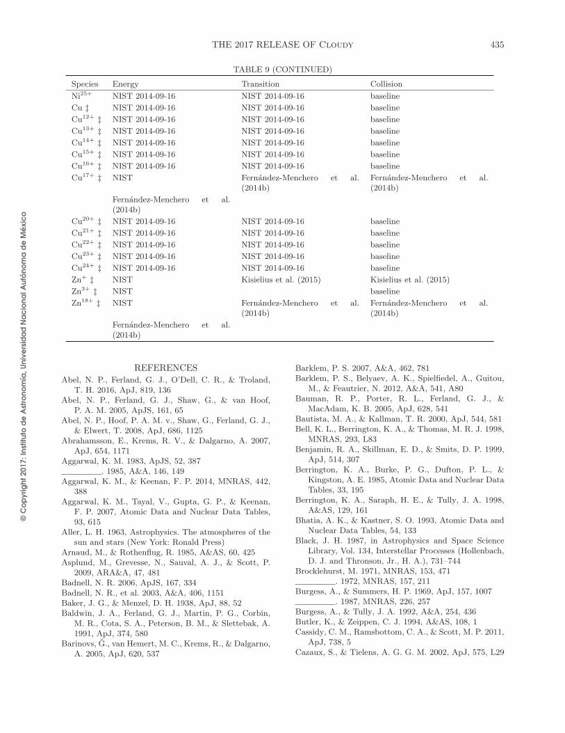
© C
op
yri
gh
t 2
01
7: In
stitu
to d
e A
stro
no
mía
, U
niv
ers
ida
d N
ac
ion
al A
utó
no
ma
de
Mé
xic
o
THE 2017 RELEASE OF Cloudy 435
TABLE 9 (CONTINUED)
Species Energy Transition Collision
Ni25+ NIST 2014-09-16 NIST 2014-09-16 baseline
Cu ‡ NIST 2014-09-16 NIST 2014-09-16 baseline
Cu12+ ‡ NIST 2014-09-16 NIST 2014-09-16 baseline
Cu13+ ‡ NIST 2014-09-16 NIST 2014-09-16 baseline
Cu14+ ‡ NIST 2014-09-16 NIST 2014-09-16 baseline
Cu15+ ‡ NIST 2014-09-16 NIST 2014-09-16 baseline
Cu16+ ‡ NIST 2014-09-16 NIST 2014-09-16 baseline
Cu17+ ‡ NIST Fernandez-Menchero et al.(2014b)
Fernandez-Menchero et al.(2014b)
Fernandez-Menchero et al.(2014b)
Cu20+ ‡ NIST 2014-09-16 NIST 2014-09-16 baseline
Cu21+ ‡ NIST 2014-09-16 NIST 2014-09-16 baseline
Cu22+ ‡ NIST 2014-09-16 NIST 2014-09-16 baseline
Cu23+ ‡ NIST 2014-09-16 NIST 2014-09-16 baseline
Cu24+ ‡ NIST 2014-09-16 NIST 2014-09-16 baseline
Zn+ ‡ NIST Kisielius et al. (2015) Kisielius et al. (2015)
Zn3+ ‡ NIST baseline
Zn18+ ‡ NIST Fernandez-Menchero et al.(2014b)
Fernandez-Menchero et al.(2014b)
Fernandez-Menchero et al.(2014b)
REFERENCES
Abel, N. P., Ferland, G. J., O’Dell, C. R., & Troland,T. H. 2016, ApJ, 819, 136
Abel, N. P., Ferland, G. J., Shaw, G., & van Hoof,P. A. M. 2005, ApJS, 161, 65
Abel, N. P., Hoof, P. A. M. v., Shaw, G., Ferland, G. J.,& Elwert, T. 2008, ApJ, 686, 1125
Abrahamsson, E., Krems, R. V., & Dalgarno, A. 2007,ApJ, 654, 1171
Aggarwal, K. M. 1983, ApJS, 52, 387. 1985, A&A, 146, 149
Aggarwal, K. M., & Keenan, F. P. 2014, MNRAS, 442,388
Aggarwal, K. M., Tayal, V., Gupta, G. P., & Keenan,F. P. 2007, Atomic Data and Nuclear Data Tables,93, 615
Aller, L. H. 1963, Astrophysics. The atmospheres of thesun and stars (New York: Ronald Press)
Arnaud, M., & Rothenflug, R. 1985, A&AS, 60, 425Asplund, M., Grevesse, N., Sauval, A. J., & Scott, P.
2009, ARA&A, 47, 481Badnell, N. R. 2006, ApJS, 167, 334Badnell, N. R., et al. 2003, A&A, 406, 1151Baker, J. G., & Menzel, D. H. 1938, ApJ, 88, 52Baldwin, J. A., Ferland, G. J., Martin, P. G., Corbin,
M. R., Cota, S. A., Peterson, B. M., & Slettebak, A.1991, ApJ, 374, 580
Barinovs, G., van Hemert, M. C., Krems, R., & Dalgarno,A. 2005, ApJ, 620, 537
Barklem, P. S. 2007, A&A, 462, 781Barklem, P. S., Belyaev, A. K., Spielfiedel, A., Guitou,
M., & Feautrier, N. 2012, A&A, 541, A80Bauman, R. P., Porter, R. L., Ferland, G. J., &
MacAdam, K. B. 2005, ApJ, 628, 541Bautista, M. A., & Kallman, T. R. 2000, ApJ, 544, 581Bell, K. L., Berrington, K. A., & Thomas, M. R. J. 1998,
MNRAS, 293, L83Benjamin, R. A., Skillman, E. D., & Smits, D. P. 1999,
ApJ, 514, 307Berrington, K. A., Burke, P. G., Dufton, P. L., &
Kingston, A. E. 1985, Atomic Data and Nuclear DataTables, 33, 195
Berrington, K. A., Saraph, H. E., & Tully, J. A. 1998,A&AS, 129, 161
Bhatia, A. K., & Kastner, S. O. 1993, Atomic Data andNuclear Data Tables, 54, 133
Black, J. H. 1987, in Astrophysics and Space ScienceLibrary, Vol. 134, Interstellar Processes (Hollenbach,D. J. and Thronson, Jr., H. A.), 731–744
Brocklehurst, M. 1971, MNRAS, 153, 471. 1972, MNRAS, 157, 211
Burgess, A., & Summers, H. P. 1969, ApJ, 157, 1007. 1987, MNRAS, 226, 257
Burgess, A., & Tully, J. A. 1992, A&A, 254, 436Butler, K., & Zeippen, C. J. 1994, A&AS, 108, 1Cassidy, C. M., Ramsbottom, C. A., & Scott, M. P. 2011,
ApJ, 738, 5Cazaux, S., & Tielens, A. G. G. M. 2002, ApJ, 575, L29
© C
op
yri
gh
t 2
01
7: In
stitu
to d
e A
stro
no
mía
, U
niv
ers
ida
d N
ac
ion
al A
utó
no
ma
de
Mé
xic
o
436 FERLAND ET AL.
. 2004, ApJ, 604, 222
. 2010, ApJ, 715, 698Chandrasekhar, S. 1957, An introduction to the study of
stellar structure. (New York, Dover Publications). 1960, Radiative transfer (New York: Dover)
Chatzikos, M., Ferland, G. J., Williams, R. J. R., Porter,R., & van Hoof, P. A. M. 2013, ApJ, 779, 122
Chatzikos, M., et al. 2015, MNRAS, 446, 1234Chekhovskoy, V. Y. 1971, J. Chem. Thermodynamics, 3,
289Chung, H.-K., Bowen, C., Fontes, C. J., Hansen, S. B.,
& Ralchenko, Y. 2013, High Energy Density Physics,9, 645
Chung, H.-K., Chen, M. H., Morgan, W. L., Ralchenko,Y., & Lee, R. W. 2005, High Energy Density Physics,1, 3
Dalgarno, A., & McCray, R. A. 1972, ARA&A, 10, 375Davidson, K. 1975, ApJ, 195, 285D’Cruz, N. L., Sarazin, C. L., & Dubau, J. 1998, ApJ,
501, 414Del Zanna, G., Storey, P. J., & Badnell, N. R. 2014a,
A&A, 566, A123Del Zanna, G., Storey, P. J., Badnell, N. R., & Mason,
H. E. 2014b, A&A, 565, A77Del Zanna, G., Storey, P. J., & Mason, H. E. 2014c, A&A,
567, A18Dere, K. P. 2007, A&A, 466, 771Dere, K. P., Landi, E., Mason, H. E., Monsignori Fossi,
B. C., & Young, P. R. 1997, A&AS, 125Draine, B. T. 2011, Physics of the Interstellar and Inter-
galactic Medium (Princeton University Press)Draine, B. T., & Bertoldi, F. 1996, ApJ, 468, 269Dufton, P. L., & Kingston, A. E. 1987, Journal of Physics
B Atomic Molecular Physics, 20, 3899Elwert, T., Ferland, G. J., Henney, W. J., & Williams,
R. J. R. 2005, in IAU Symposium, Vol. 235, IAU Sym-posium, 132P
Fabian, A. C., Nulsen, P. E. J., & Canizares, C. R. 1984,Nature, 310, 733
Ferland, G. J. 1980, PASP, 92, 596. 2003, ARA&A, 41, 517
Ferland, G. J., Henney, W. J., O’Dell, C. R., & Peimbert,M. 2016, RMxAA, 52, 261
Ferland, G. J., Henney, W. J., O’Dell, C. R., Porter,R. L., van Hoof, P. A. M., & Williams, R. J. R. 2012,ApJ, 757, 79
Ferland, G. J., Korista, K. T., Verner, D. A., Ferguson,J. W., Kingdon, J. B., & Verner, E. M. 1998, PASP,110, 761
Ferland, G. J., Peterson, B. M., Horne, K., Welsh, W. F.,& Nahar, S. N. 1992, ApJ, 387, 95
Ferland, G. J., & Rees, M. J. 1988, ApJ, 332, 141Ferland, G. J., & Williams, R. J. R. 2016, in Modern
Methods in Collisional-Radiative Modeling of Plas-mas, ed. Y. Ralchenko (Cham: Springer InternationalPublishing), 153–180
Ferland, G. J., et al. 2013, RMxAA, 49, 137
Fernandez-Menchero, L., Del Zanna, G., & Badnell, N. R.2014a, A&A, 566, A104
. 2014b, A&A, 572, A115Flower, D. R., Le Bourlot, J., Pineau des Forets, G., &
Roueff, E. 2000, MNRAS, 314, 753Froese Fischer, C., & Tachiev, G. 2004, Atomic Data and
Nuclear Data Tables, 87, 1Froese Fischer, C., Tachiev, G., & Irimia, A. 2006,
Atomic Data and Nuclear Data Tables, 92, 607Galavis, M. E., Mendoza, C., & Zeippen, C. J. 1995,
A&AS, 111, 347. 1997, A&AS, 123, 159
Garstang, R. H. 1993, in Bulletin of the American As-tronomical Society, Vol. 25, American AstronomicalSociety Meeting Abstracts #182 (Washington, AAS),934
Glover, S. C. O., & Abel, T. 2008, MNRAS, 388, 1627Gnat, O. 2017, ApJS, 228, 11Gnat, O., & Ferland, G. J. 2012, ApJS, 199, 20Gnat, O., & Sternberg, A. 2007, ApJS, 168, 213Goldsmith, P. F., Langer, W. D., Pineda, J. L., &
Velusamy, T. 2012, ApJS, 203, 13Graney, C. M., & Sarazin, C. L. 1990, ApJ, 364, 561Grieve, M. F. R., & Ramsbottom, C. A. 2012, MNRAS,
424, 2461Griffin, D. C., Mitnik, D. M., & Badnell, N. R. 2001,
Journal of Physics B Atomic Molecular Physics, 34,4401
Guzman, F., Badnell, N. R., Chatzikos, M., van Hoof,P. A. M., Williams, R. J. R., & Ferland, G. J. 2017a,MNRAS, 467, 3944
Guzman, F., Badnell, N. R., Williams, R. J. R., vanHoof, P. A. M., Chatzikos, M., & Ferland, G. J. 2016,MNRAS, 459, 3498
. 2017b, MNRAS, 464, 312Haardt, F., & Madau, P. 2012, ApJ, 746, 125He, X., Chen, A., Zhang, C., & Li, B. 1990, Journal of
Physics B Atomic Molecular Physics, 23, 661Heise, C., Smith, P. L., & Calamai, A. G. 1995, ApJ, 451,
L41Henney, W. J., Arthur, S. J., Williams, R. J. R., & Fer-
land, G. J. 2005, ApJ, 621, 328Henney, W. J., Williams, R. J. R., Ferland, G. J., Shaw,
G., & O’Dell, C. R. 2007, ApJ, 671, L137Hollenbach, D., & McKee, C. F. 1989, ApJ, 342, 306Hubeny, I., & Mihalas, D. 2014, Theory of Stellar Atmo-
spheres (Princeton, NJ: Princeton University Press)Hudson, C. E., Norrington, P. H., Ramsbottom, C. A.,
& Scott, M. P. 2012a, A&A, 537, A12Hudson, C. E., Ramsbottom, C. A., & Scott, M. P. 2012b,
ApJ, 750, 65Hummer, D. G., & Storey, P. J. 1987, MNRAS, 224, 801
. 1998, MNRAS, 297, 1073Irons, F. E. 1978, MNRAS, 182, 705Izotov, Y. I., Thuan, T. X., & Guseva, N. G. 2014,
Monthly Notices of the Royal Astronomical Society,445, 778
© C
op
yri
gh
t 2
01
7: In
stitu
to d
e A
stro
no
mía
, U
niv
ers
ida
d N
ac
ion
al A
utó
no
ma
de
Mé
xic
o
THE 2017 RELEASE OF Cloudy 437
Jaquet, R., Staemmler, V., Smith, M. D., & Flower, D. R.1992, Journal of Physics B Atomic Molecular Physics,25, 285
Johnson, C. T., Burke, P. G., & Kingston, A. E. 1987,Journal of Physics B Atomic Molecular Physics, 20,2553
Jordan, C. 1969, MNRAS, 142, 501Kisielius, R., Kulkarni, V. P., Ferland, G. J., Bog-
danovich, P., & Lykins, M. L. 2014, ApJ, 780, 76Kisielius, R., Kulkarni, V. P., Ferland, G. J., Bog-
danovich, P., Som, D., & Lykins, M. L. 2015, ApJ,804, 76
Kisielius, R., Storey, P. J., Ferland, G. J., & Keenan,F. P. 2009, MNRAS, 397, 903
Kramida, A., Yu. Ralchenko, Reader, J., & andNIST ASD Team. 2014, NIST Atomic Spec-tra Database (ver. 5.2), [Online]. Available:http://physics.nist.gov/asd [2014, November28]. National Institute of Standards and Technology,Gaithersburg, MD.
Krems, R. V., Jamieson, M. J., & Dalgarno, A. 2006,ApJ, 647, 1531
Krueger, T. K., & Czyzak, S. J. 1970, Proceedings of theRoyal Society of London Series A, 318, 531
Kwon, D.-H., & Savin, D. W. 2014, ApJ, 784, 13Kwong, H. S., Johnson, B. C., Smith, P. L., & Parkinson,
W. H. 1983, Phys. Rev. A, 27, 3040Laha, S., et al. 2016, MNRAS, 455, 3405Landi, E., Del Zanna, G., Young, P. R., Dere, K. P., &
Mason, H. E. 2012, ApJ, 744, 99Laor, A., & Draine, B. T. 1993, ApJ, 402, 441Le Bourlot, J., Le Petit, F., Pinto, C., Roueff, E., & Roy,
F. 2012, A&A, 541, A76Le Bourlot, J., Pineau des Forets, G., & Flower, D. R.
1999, MNRAS, 305, 802Le Teuff, Y. H., Millar, T. J., & Markwick, A. J. 2000,
A&AS, 146, 157Lennon, D. J., & Burke, V. M. 1994, A&AS, 103, 273Liang, G. Y., & Badnell, N. R. 2010, A&A, 518, A64Liang, G. Y., Whiteford, A. D., & Badnell, N. R. 2009,
A&A, 500, 1263Lique, F. 2015, MNRAS, 453, 810Luridiana, V., Simon-Dıaz, S., Cervino, M., Delgado,
R. M. G., Porter, R. L., & Ferland, G. J. 2009, ApJ,691, 1712
Lykins, M. L., Ferland, G. J., Porter, R. L., van Hoof,P. A. M., Williams, R. J. R., & Gnat, O. 2013,MNRAS, 429, 3133
Lykins, M. L., et al. 2015, ApJ, 807, 118Mao, J., Kaastra, J., & Badnell, N. R. 2017, A&A, 599,
A10McElroy, D., Walsh, C., Markwick, A. J., Cordiner,
M. A., Smith, K., & Millar, T. J. 2013, A&A, 550,A36
McLaughlin, B. M., Lee, T.-G., Ludlow, J. A., Landi, E.,Loch, S. D., Pindzola, M. S., & Ballance, C. P. 2011,Journal of Physics B Atomic Molecular Physics, 44,175206
Mehdipour, M., Kaastra, J. S., & Kallman, T. 2016,A&A, 596, A65
Mendoza, C. 1983, in IAU Symposium, Vol. 103, Plane-tary Nebulae, ed. D. R. Flower, 143–172
Menzel, D. H., & Pekeris, C. L. 1935, MNRAS, 96, 77Monteiro, T. S., & Flower, D. R. 1987, MNRAS, 228, 101Nikolic, D., Gorczyca, T. W., Korista, K. T., Ferland,
G. J., & Badnell, N. R. 2013, ApJ, 768, 82Osorio, Y., Barklem, P. S., Lind, K., Belyaev, A. K.,
Spielfiedel, A., Guitou, M., & Feautrier, N. 2015,A&A, 579, A53
Osterbrock, D. E., & Ferland, G. J. 2006, Astrophysicsof gaseous nebulae and active galactic nuclei, 2nd. ed.(Sausalito, CA: University Science Books)
Pelan, J., & Berrington, K. A. 1995, A&AS, 110, 209Pengelly, R. M., & Seaton, M. J. 1964, MNRAS, 127, 165Pequignot, D. 1986, in Model Nebulae, ed. D. Pequignot,
363Pequignot, D. 1990, A&A, 231, 499Piron, R., et al. 2017, High Energy Density Physics, 23,
38Podobedova, L. I., Kelleher, D. E., & Wiese, W. L. 2009,
Journal of Physical and Chemical Reference Data, 38,171
Porter, R. L., Bauman, R. P., Ferland, G. J., &MacAdam, K. B. 2005, ApJ, 622, L73
Porter, R. L., & Ferland, G. J. 2007, ApJ, 664, 586Porter, R. L., Ferland, G. J., Kraemer, S. B., Armen-
trout, B. K., Arnaud, K. A., & Turner, T. J. 2006,PASP, 118, 920
Porter, R. L., Ferland, G. J., & MacAdam, K. B. 2007,ApJ, 657, 327
Porter, R. L., Ferland, G. J., Storey, P. J., & Detisch,M. J. 2012, MNRAS, 425, L28
Ramsbottom, C. A., Bell, K. L., & Keenan, F. P. 1997,MNRAS, 284, 754
Rollig, M., Szczerba, R., Ossenkopf, V., & Gluck, C.2013, A&A, 549, A85
Rollig, M., et al. 2007, A&A, 467, 187Roueff, E., & Le Bourlot, J. 1990, A&A, 236, 515Rouleau, F., & Martin, P. G. 1991, ApJ, 377, 526Rybicki, G. B. 1984, in Methods in Radiative Transfer,
ed. W. Kalkofen (Cambridge University Press), 21–64Rybicki, G. B., & Lightman, A. P. 1979, Radia-
tive processes in astrophysics (New York, Wiley-Interscience), 393 p.
Saraph, H. E., & Storey, P. J. 1996, A&AS, 115, 151Saraph, H. E., & Tully, J. A. 1994, A&AS, 107, 29Schirmer, M. 2016, PASP, 128, 114001Schoier, F. L., van der Tak, F. F. S., van Dishoeck, E. F.,
& Black, J. H. 2005, A&A, 432, 369Schroder, K., Staemmler, V., Smith, M. D., Flower,
D. R., & Jaquet, R. 1991, Journal of Physics BAtomic Molecular Physics, 24, 2487
Seaton, M. 1987, Journal of Physics B Atomic MolecularPhysics, 20, 6363
Seaton, M. J. 1959, MNRAS, 119, 81

© C
op
yri
gh
t 2
01
7: In
stitu
to d
e A
stro
no
mía
, U
niv
ers
ida
d N
ac
ion
al A
utó
no
ma
de
Mé
xic
o
438 FERLAND ET AL.
. 1962, Proceedings of the Physical Society,79, 1105
. 1964, MNRAS, 127, 177
Sellgren, K., Tokunaga, A. T., & Nakada, Y. 1990, ApJ,349, 120
Shaw, G., Ferland, G. J., Abel, N. P., Stancil, P. C., &van Hoof, P. A. M. 2005, ApJ, 624, 794
Spitzer, L. 1962, Physics of Fully Ionized Gases (2nd edi-tion) (New York: Interscience)
. 1978, Physical processes in the interstellarmedium (New York Wiley-Interscience), 333 p.
Spitzer, L. J., & Tomasko, M. G. 1968, ApJ, 152, 971
Staemmler, V., & Flower, D. R. 1991, Journal of PhysicsB Atomic Molecular Physics, 24, 2343
Storey, P. J., & Hummer, D. G. 1995, MNRAS, 272,41, on the web at http://adc.gsfc.nasa.gov/adc-cgi/cat.pl?/catalogs/6/6064/
Storey, P. J., & Sochi, T. 2016, MNRAS, 459, 2558
Storey, P. J., Sochi, T., & Badnell, N. R. 2014, MNRAS,441, 3028
Storey, P. J., & Zeippen, C. J. 2000, MNRAS, 312, 813Storey, P. J., Zeippen, C. J., & Sochi, T. 2015, ArXiv
e-printsSummers, H. P., et al. 2006, Plasma Physics and Con-
trolled Fusion, 48, 263Sunyaev, R. A., & Vainshtein, L. A. 1968, Astro-
phys. Lett., 1, 69Sutherland, R. S., & Dopita, M. A. 1993, ApJS, 88, 253
Tachiev, G., & Froese Fischer, C. 2001, Canadian Journalof Physics, 79, 955
Tayal, S. S. 1997, Atomic Data and Nuclear Data Tables,67, 331
. 2006, ApJS, 163, 207
. 2008, A&A, 486, 629Tayal, S. S., & Zatsarinny, O. 2010, ApJS, 188, 32
Tielens, A. G. G. M. 2005, The Physics and Chemistry ofthe Interstellar Medium (Cambridge, UK: CambridgeUniversity Press)
Nicholas P. Abel: Department of Physics, University of Cincinnati, 4200 Clermont College Drive, Batavia, Ohio,45103, USA ([email protected]).
N. R. Badnell: Department of Physics, University of Strathclyde, Glasgow, G4 0NG, UK ([email protected]).
M. Chatzikos, F. Guzman, Gary J. Ferland and Matthew L. Lykins: Department of Physics and Astron-omy, University of Kentucky, Lexington, KY 40506, USA ([email protected], [email protected], [email protected], [email protected]).
Francis P. Keenan: Astrophysics Research Centre, School of Mathematics and Physics, Queen’s UniversityBelfast, Belfast BT7 1NN, Northern Ireland, U.K. ([email protected]).
Ryan L. Porter and Phillip Stancil: Department of Physics and Astronomy and Center for SimulationalPhysics, The University of Georgia, Athens, Georgia 30602-2451, USA ([email protected], [email protected]).
Peter A. M. van Hoof: Royal Observatory of Belgium, Ringlaan 3, 1180 Brussels, Belgium ([email protected]).Robin J. R. Williams: AWE plc, Aldermaston, Reading RG7 4PR, UK ([email protected]).
Tielens, A. G. G. M., & Hollenbach, D. 1985, ApJ, 291,722
van Hoof, P. A. M., Ferland, G. J., Williams, R. J. R.,Volk, K., Chatzikos, M., Lykins, M., & Porter, R. L.2015, MNRAS, 449, 2112
van Hoof, P. A. M., Weingartner, J. C., Martin, P. G.,Volk, K., & Ferland, G. J. 2004, MNRAS, 350, 1330
van Hoof, P. A. M., Williams, R. J. R., Volk, K.,Chatzikos, M., Ferland, G. J., Lykins, M., Porter,R. L., & Wang, Y. 2014, MNRAS, 444, 420
Verner, D. A., Ferland, G. J., Korista, K. T., & Yakovlev,D. G. 1996, ApJ, 465, 487
Verner, E. M., Verner, D. A., Korista, K. T., Ferguson,J. W., Hamann, F., & Ferland, G. J. 1999, ApJS, 120,101
Voronov, G. S. 1997, Atomic Data and Nuclear Data Ta-bles, 65, 1
Vrinceanu, D., & Flannery, M. R. 2001a, Phys. Rev. A,63, 032701
. 2001b, Journal of Physics B Atomic Molec-ular Physics, 34, L1
Vrinceanu, D., Onofrio, R., & Sadeghpour, H. R. 2012,ApJ, 747, 56
Wang, S., & McConkey, J. W. 1992, Journal of PhysicsB Atomic Molecular Physics, 25, 5461
Wang, Y., Ferland, G. J., Lykins, M. L., Porter, R. L.,van Hoof, P. A. M., & Williams, R. J. R. 2014,MNRAS, 440, 3100
Wasson, I. R., Ramsbottom, C. A., & Scott, M. P. 2011,ApJS, 196, 24
Wiesenfeld, L., & Goldsmith, P. F. 2014, ApJ, 780, 183Williams, R. J. R., Guzman, F., Badnell, N. R., van
Hoof, P. A. M., Chatzikos, M., & Ferland, G. J. 2017,Journal of Physics B Atomic Molecular Physics, 50,115201
Witthoeft, M. C., & Badnell, N. R. 2008, A&A, 481, 543Wrathmall, S. A., Gusdorf, A., & Flower, D. R. 2007,
MNRAS, 382, 133Zhang, H. 1996, A&AS, 119, 523