Embed Size (px)
Citation preview
REVIEW:
• ELECTRIC FORCE, ELECTRIC FIELD, • ELECTRIC FIELD LINES, ELECTRIC FLUX, GAUSS’S LAW, • ELECTRIC POTENTIAL, • CONTINUOUS CHARGE DISTRIBUTIONS (ELECTRIC FIELD, ELECTRIC
POTENTIAL, GAUSS’S LAW), • ELECTRIC CURRENT, • MAGNETIC FORCE ON MOVING CHARGES AND WIRES, • BIO-SAVART-LAW, • FORCE BETWEEN PARALLEL CURRENT CARRYING WIRES
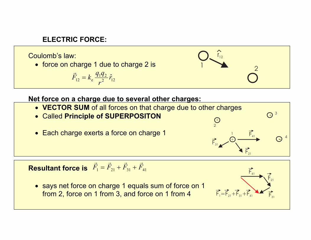
ELECTRIC FORCE: Coulomb’s law: • force on charge 1 due to charge 2 is
12221
e12 rrqqkF =
r
Net force on a charge due to several other charges: • VECTOR SUM of all forces on that charge due to other charges • Called Principle of SUPERPOSITON
• Each charge exerts a force on charge 1
Resultant force is 4131211 FFFF
rrrr++=
• says net force on charge 1 equals sum of force on 1
from 2, force on 1 from 3, and force on 1 from 4

ELECTRIC FIELD
• If the force on 0q at a point is Fr
, then electric field at that point is 0q
FEr
r=
• If the electric field at a point is Er
, then the force on 0q at point is EqFrr
0=
• Electric field at P due to a point charge is rrqkE ˆ
2eP =r
o Unit vector r points from q → P
• Electric field points away from positive charge • Electric field points toward negative charge

Superposition: Total E
r at point P due to an arrangement of point charges is the VECTOR SUM
of the electric field contributions from all charges around P • Total electric field at P is:
43212
ˆEEEE
rrqkE
i i
iieT
rrrrr+++== ∑
o iq is the charge at i
o ir is the distance from iq → P
o ir is the unit vector from iq → P
o the sum is a VECTOR SUM
Did example with electric dipole

ELECTRIC FIELD LINES: • E
r vector at a point in space is tangent to the EFL through that point
• “Density” of EFL is proportional to E (magnitude) in that region
o Larger E→ closer packing of lines
• EFL start on positive charges and end on negative charges
• Number of EFL starting/ending on charge is proportional to its magnitude
• Electric field lines do not cross

Looked at motion of a particle in a uniform electric field:
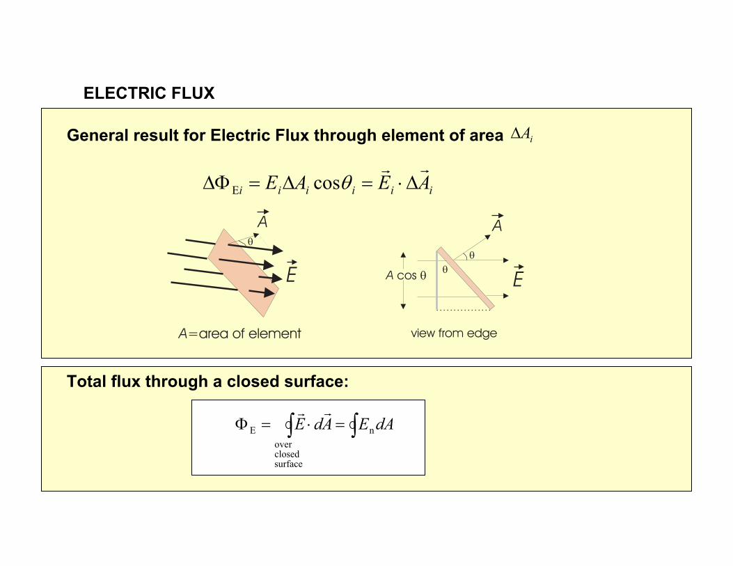
ELECTRIC FLUX
General result for Electric Flux through element of area iA∆
iiiiii AEAErr
∆⋅=∆=∆Φ θcosE
Total flux through a closed surface:
∫∫ =⋅=Φ dAEAdE n
surfaceclosedover
E
rr

GAUSS’S LAW (general statement):
0
enclosed
surfaceclosed
e εqAdE∫ =⋅=Φ
rr
• Powerful way to calculate electric field if we can factor nE out of integral
o Trick is to choose surface so that nE is uniform over all or part of surface No charge inside: • net number of lines leaving = 0 • all lines go through
Positive charge inside: • non-zero net number of lines leaving • lines start on charge inside sphere
Used Gauss’s Law to calculate electric field around a point charge

ELECTRIC POTENTIAL Difference in electric potential between points A and B is:
0qUVVV AB
∆=−=∆
SO: ∫ ⋅−=−=∆B
AAB sdEVVV rr
o Potential difference between two points depends on electric field o Note sign and order of integration limits
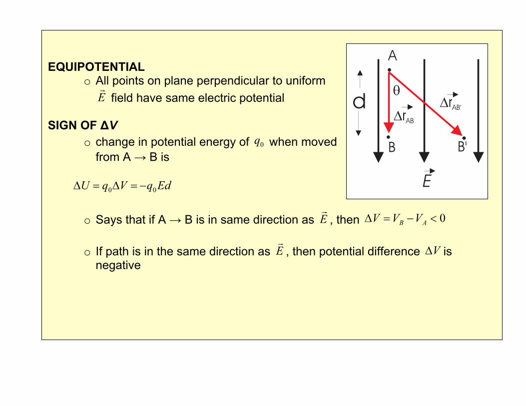
EQUIPOTENTIAL o All points on plane perpendicular to uniform
Er
field have same electric potential
SIGN OF ∆V o change in potential energy of 0q when moved
from A → B is
EdqVqU 00 −=∆=∆ o Says that if A → B is in same direction as E
r, then 0<−=∆ AB VVV
o If path is in the same direction as E
r, then potential difference V∆ is
negative
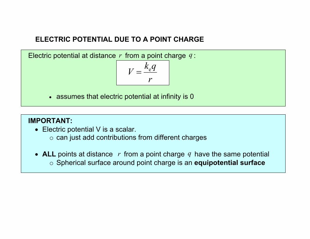
ELECTRIC POTENTIAL DUE TO A POINT CHARGE Electric potential at distance r from a point charge q :
rqkV e=
• assumes that electric potential at infinity is 0 IMPORTANT: • Electric potential V is a scalar.
o can just add contributions from different charges
• ALL points at distance r from a point charge q have the same potential o Spherical surface around point charge is an equipotential surface

Electric Potential due to multiple point charges: SUPERPOSITION • Electric potential at P is
∑=i i
i
rqkV e
o Not a vector sum. Contributions to V add as scalars
Can get components of E
r from derivatives of V
Implies: dxdVEx −= dy
dVEy −= dzdVEz −=
• Says: E
r is always perpendicular to equipotential surfaces
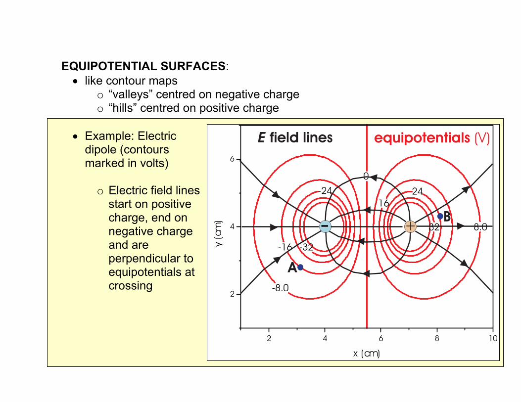
EQUIPOTENTIAL SURFACES: • like contour maps
o “valleys” centred on negative charge o “hills” centred on positive charge
• Example: Electric dipole (contours marked in volts)
o Electric field lines
start on positive charge, end on negative charge and are perpendicular to equipotentials at crossing
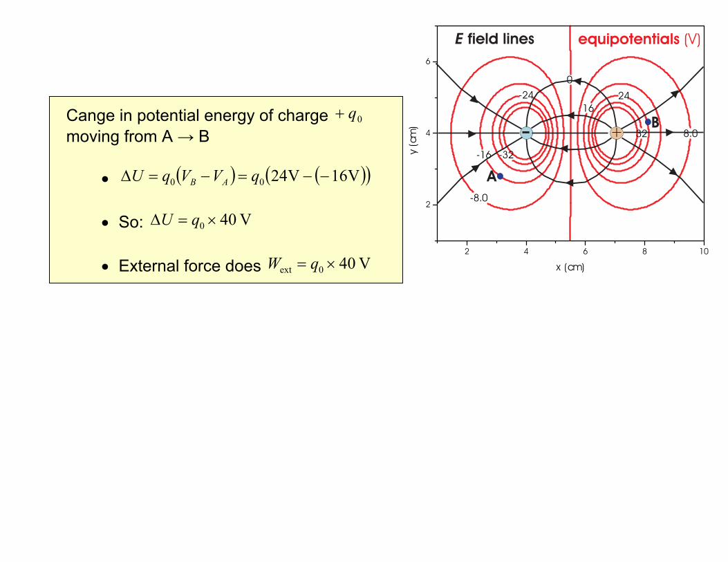
Cange in potential energy of charge 0q+ moving from A → B
• ( ) ( )( )V16V2400 −−=−=∆ qVVqU AB • So: V 400 ×=∆ qU • External force does V 400ext ×= qW
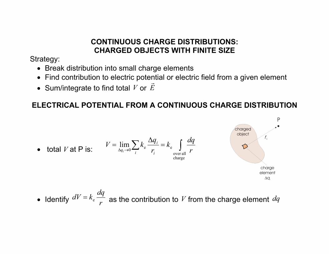
CONTINUOUS CHARGE DISTRIBUTIONS: CHARGED OBJECTS WITH FINITE SIZE
Strategy: • Break distribution into small charge elements • Find contribution to electric potential or electric field from a given element • Sum/integrate to find total V or E
r
ELECTRICAL POTENTIAL FROM A CONTINUOUS CHARGE DISTRIBUTION
• total V at P is: ∫∑ =∆
=→∆
chargeallover
ee0lim
rdqk
rqkV
i i
i
qi
• Identify rdqkdV e= as the contribution to V from the charge element dq
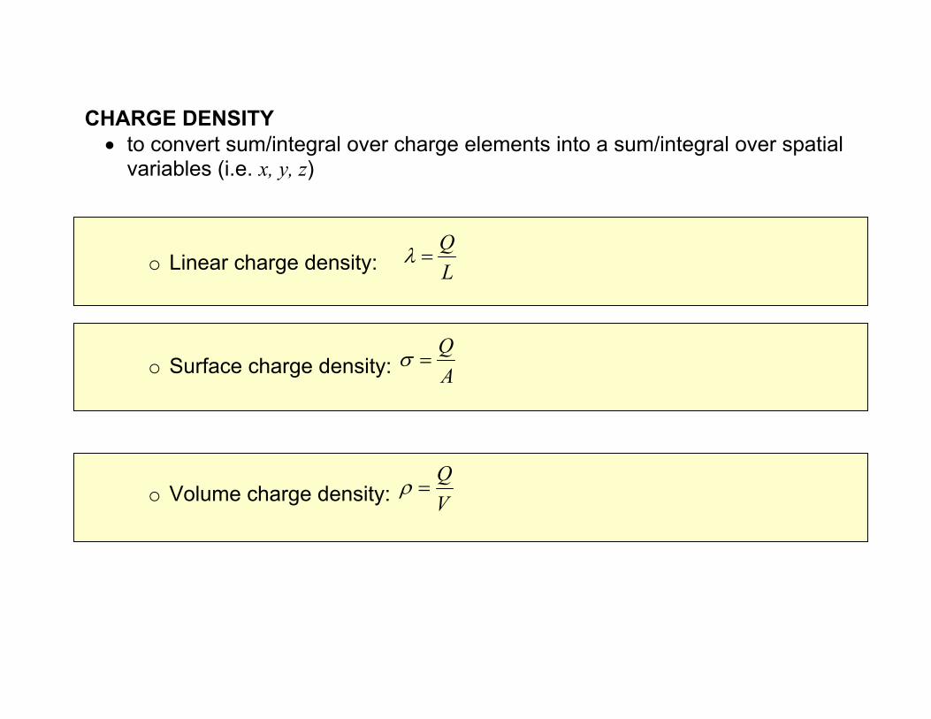
CHARGE DENSITY • to convert sum/integral over charge elements into a sum/integral over spatial
variables (i.e. x, y, z)
o Linear charge density: LQ
=λ
o Surface charge density: AQ
=σ
o Volume charge density: VQ
=ρ

ELECTRIC FIELDS DUE TO CONTINUOUS CHARGE DISTRIBUTIONS Approach: • Break charge distribution into small elements (treat each as a point charge) • Write vector sum of contributions from elements • Take limit as elements become infinitesimally small → INTEGRAL
o ir is unit vector pointing from iq∆ toward P
o iEr
∆ is the contribution to Er
due to iq∆
∫
∑
=
∆=
→∆
rrdqk
rrqkE
ii
i
iqi
ˆ
ˆlim
2e
2e0
r
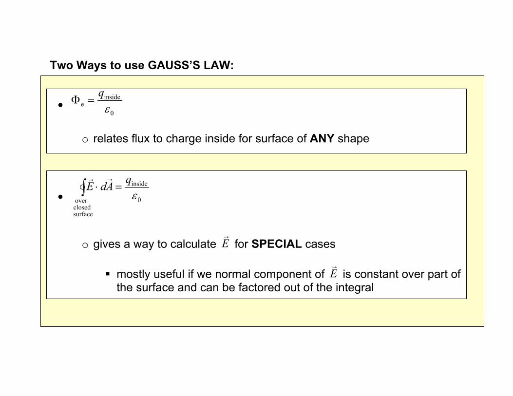
Two Ways to use GAUSS’S LAW:
• 0
insidee ε
q=Φ
o relates flux to charge inside for surface of ANY shape
• 0
inside
surface closed over ε
qAdE =⋅∫rr
o gives a way to calculate E
r for SPECIAL cases
mostly useful if we normal component of E
r is constant over part of
the surface and can be factored out of the integral

Using Gauss’s law to calculate Electric Field Er
• Must know direction of electric field from symmetry of problem
o radial (spherical symmetry) for point charge
o radial (cylindrical symmetry) for a long line of
charge
o uniform for a large flat sheet of charge

• Must choose Gaussian surface that allows us to calculate ∫ ⋅=Φ
surface closed over
e AdErr
o Must be able to factor Er
out of flux integral in region of space where we want to find electric field
Two cases for which we can evaluate ∫ ⋅surface
AdErr
for all or part of surface
• E
r uniform and perpendicular to part or all of Gaussian surface
o then flux is ∫ =⋅ AEAdE n
rr for that part of the surface
• Er
parallel (tangent) to part of the Gaussian surface

CONDUCTORS IN ELECTROSTATIC EQUILIBRIUM (19.11) PROPERTIES: ISOLATED CONDUCTOR IN ELECTROSTATIC EQUILIBRIUM
1st: 0=E
r everywhere inside a conductor
• Must be true or else charges would move until 0=E
r
2nd: Any NET CHARGE on conductor must be on surface • can prove with Gauss’s Law
ANY NET CHARGE ON THE CONDUCTOR MUST BE ON THE SURFACE
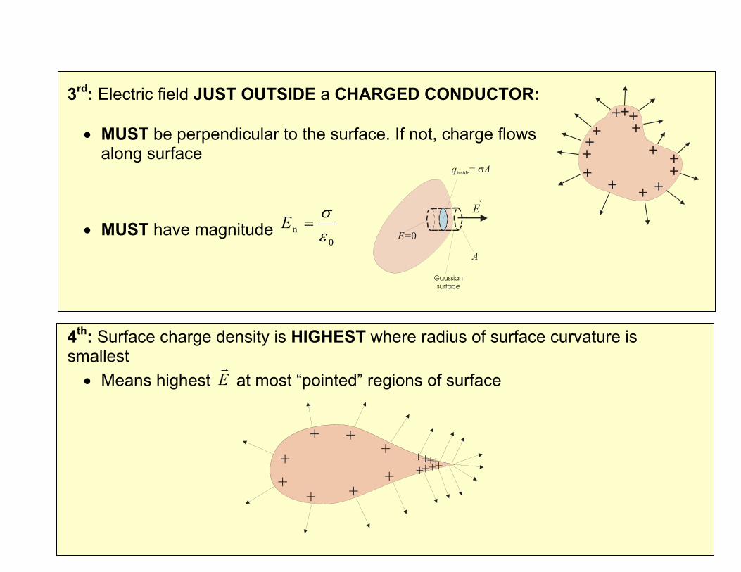
3rd: Electric field JUST OUTSIDE a CHARGED CONDUCTOR: • MUST be perpendicular to the surface. If not, charge flows
along surface
• MUST have magnitude 0
n εσ
=E
4th: Surface charge density is HIGHEST where radius of surface curvature is smallest • Means highest E
r at most “pointed” regions of surface

ELECTRIC POTENTIAL AT THE SURFACE OF AND INSIDE CHARGED CONDUCTORS (text section 20.6)
• ⊥E
rsurface means that the surface is an equipotential
• 0=E
r inside says potential V inside conductor must be
same as potential V at surface
o entire conductor is an equipotential
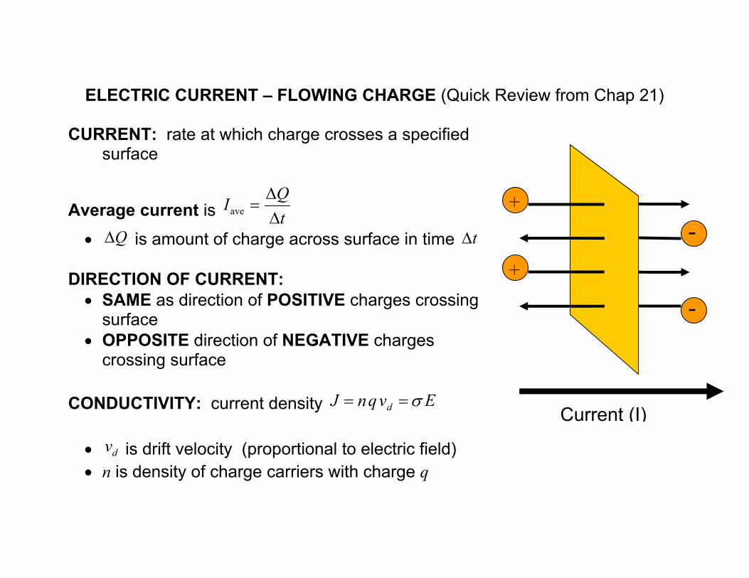
ELECTRIC CURRENT – FLOWING CHARGE (Quick Review from Chap 21)
CURRENT: rate at which charge crosses a specified surface
Average current is tQI∆∆
=ave
• Q∆ is amount of charge across surface in time t∆ DIRECTION OF CURRENT: • SAME as direction of POSITIVE charges crossing
surface • OPPOSITE direction of NEGATIVE charges
crossing surface CONDUCTIVITY: current density EvqnJ d σ== • dv is drift velocity (proportional to electric field) • n is density of charge carriers with charge q
+
+
-
-
Current (I)
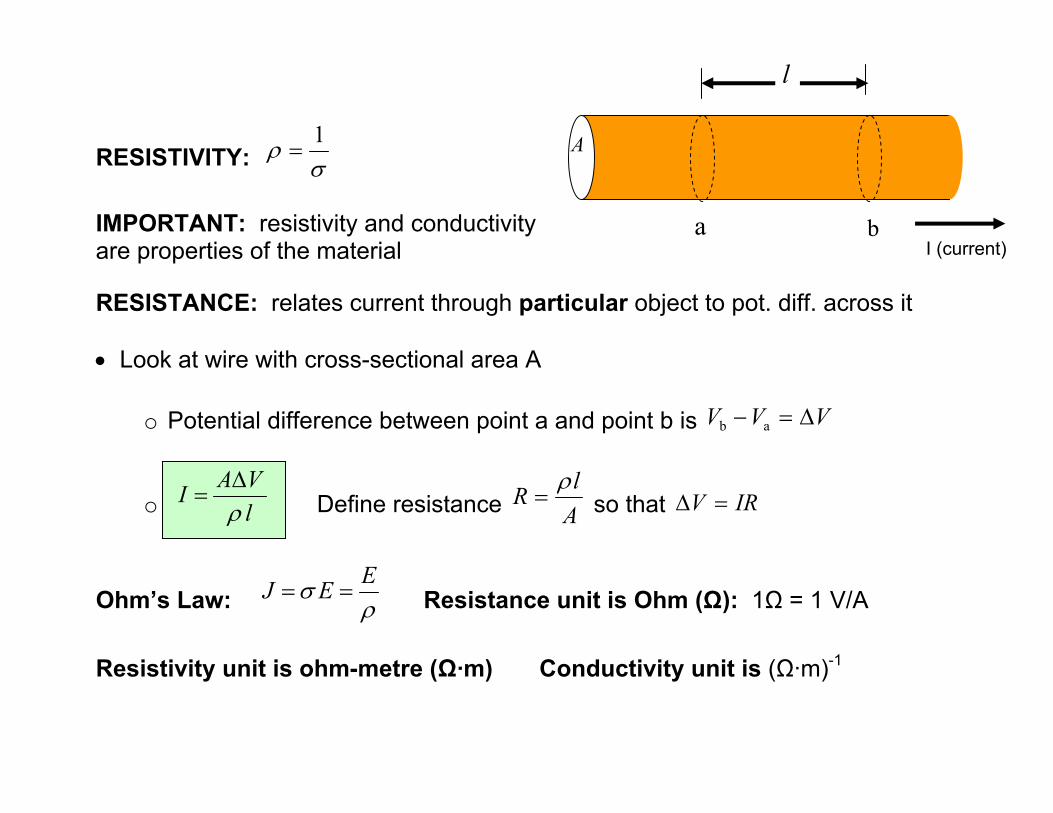
RESISTIVITY: σρ 1=
IMPORTANT: resistivity and conductivity are properties of the material RESISTANCE: relates current through particular object to pot. diff. across it • Look at wire with cross-sectional area A
o Potential difference between point a and point b is VVV ∆=− ab
o lVAI
ρ∆
= Define resistance AlR ρ
= so that IRV =∆
Ohm’s Law: ρσ EEJ == Resistance unit is Ohm (Ω): 1Ω = 1 V/A
Resistivity unit is ohm-metre (Ω·m) Conductivity unit is (Ω·m)-1
A
I (current) a b
l
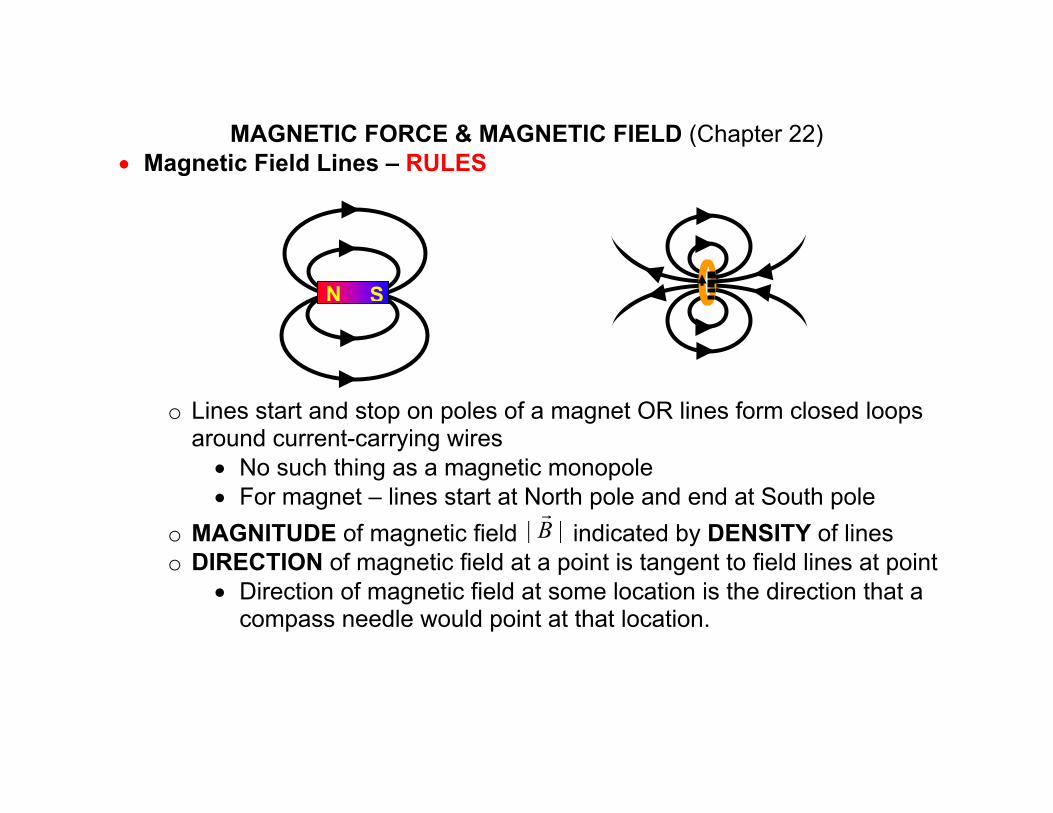
MAGNETIC FORCE & MAGNETIC FIELD (Chapter 22) • Magnetic Field Lines – RULES
o Lines start and stop on poles of a magnet OR lines form closed loops around current-carrying wires • No such thing as a magnetic monopole • For magnet – lines start at North pole and end at South pole
o MAGNITUDE of magnetic field || Br
indicated by DENSITY of lines o DIRECTION of magnetic field at a point is tangent to field lines at point
• Direction of magnetic field at some location is the direction that a compass needle would point at that location.
N S
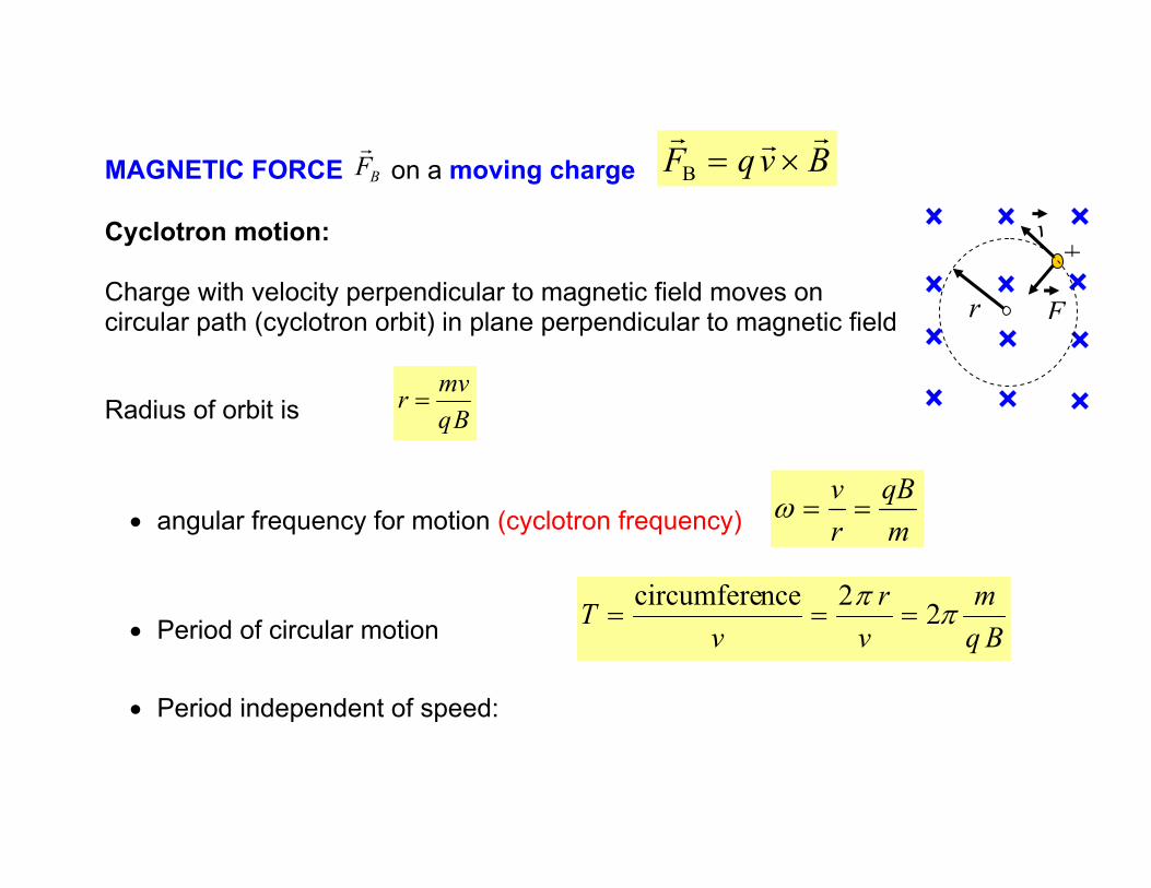
MAGNETIC FORCE BFr
on a moving charge BvqFrrr
×=B Cyclotron motion: Charge with velocity perpendicular to magnetic field moves on circular path (cyclotron orbit) in plane perpendicular to magnetic field
Radius of orbit is Bqmvr =
• angular frequency for motion (cyclotron frequency) mqB
rv==ω
• Period of circular motion Bqm
vr
vT ππ 22ncecircumfere
===
• Period independent of speed:
F
+v
r

Devices that use magnetic force on a moving charge (22.4)
In space with Er
and Br
, force on moving charge is Force) (Lorentz BvqEqFrrrr
×+= VELOCITY SELECTOR • Contains region of space with uniform electric and magnetic fields
o perpendicular to each other o perpendicular to path of charged particle
• In selector region:
o BvqFrrr
×=B is “up” by RHR o EqF
rr=E is “down”
• Net force on charge is zero IF EqBvq =
• So particles with speed BEv= are undeflected
+ + + + + + +
- - - - - - -
Barrier with hole E (down)
B (into screen)
+q v

MASS SPECTROMETER
• 1st: ionize molecules and fragments • 2nd: use velocity selector to pick out
fragments with sss BEv /=
• 3rd: inject ions with speed sv into uniform Br
with magnitude 0B
o Radius of path is 0Bq
vmr s=
• SO: s
s
EBrB
qm 0=
+ + + + + + +
- - - - - - -
velocity selectorBs, Es
+qv
+qvs
Detector
r
B0

CYCLOTRON – device to accelerate charged particles to high energy • for charge q in uniform B
r
o found Bqvmr =
o period of orbit is: Bqm
vr
vcircumfT ππ 22.
===
• NOTICE: period (i.e. timing of “kick”) does NOT depend on speed
alternating voltage source
• Potential difference across gap changes each time particle reaches gap
o “kick” raises K by q∆V
+q
Bup
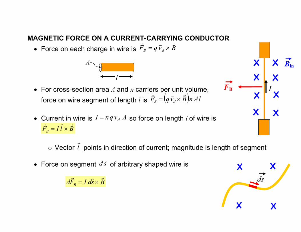
MAGNETIC FORCE ON A CURRENT-CARRYING CONDUCTOR • Force on each charge in wire is BvqF dB
rrr×=
• For cross-section area A and n carriers per unit volume,
force on wire segment of length l is ( ) lAnBvqF dB
rrr×=
• Current in wire is AvqnI d= so force on length l of wire is
BlIFB
rrr×=
o Vector l
r points in direction of current; magnitude is length of segment
• Force on segment sd r of arbitrary shaped wire is
BsdIFd B
rrr×=
I
Bin
FB
l
A
ds

Magnetic Dipole Moment • For current I circulating around loop of area A
o AIrr
=µ is the magnetic dipole moment of the loop o Magnitude: IA=µ o Direction:
• vector µr
perpendicular to the plane of the loop • direction by Right-hand rule:
• fingers curl in direction of current • thumb shows direction of µ
r
• Units of magnetic dipole moment: A·m2 • For a coil of n loops, nIA=µ
I A
µ = IA
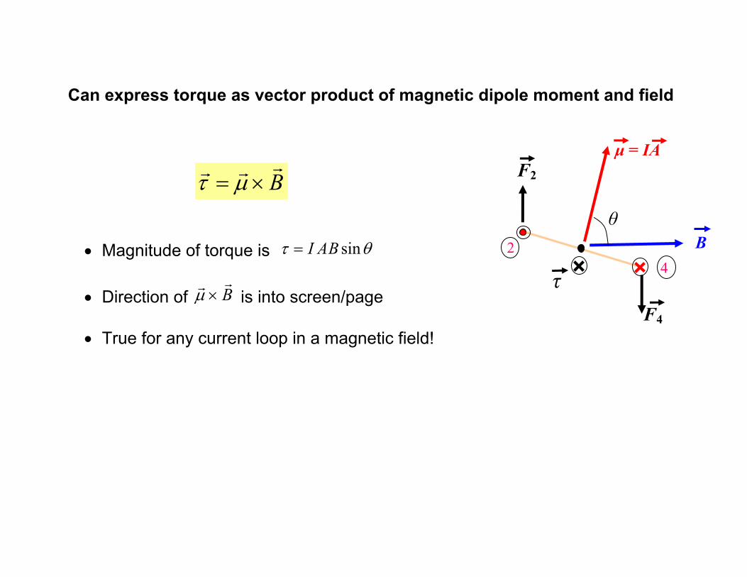
Can express torque as vector product of magnetic dipole moment and field
Brrr
×= µτ • Magnitude of torque is θτ sinBAI= • Direction of B
rr×µ is into screen/page
• True for any current loop in a magnetic field!
2 4
B
F2
F4
θ
µ = IA
τ

BIOT-SAVART LAW: 20 ˆ
4 rrsdI
Bd×
=rr
πµ
• For drawing, direction of rsd ˆ×
r is out of screen/page
o So Bd
r at P due to sdr points out of screen/page
• Magnitude θsinˆ dsrsd =×
r
o For a given r, contributions Bd
r from sdr are maximum for points on
plane perpendicular to sdr
o Current in sdr makes NO contribution to Bdr
at points along direction sdr
I
ds
r
P
θ
r

MAGNETIC FIELD AROUND A LONG (INFINITE) WIRE • Result of using Biot-Savart Law:
o Magnetic field lines circle wire → no component of Br
parallel to wire
• Magnitude of Br
inversely proportional to perpendicular a distance from wire
aIB
πµ2
0=r
(IMPORTANT RESULT)
• Direction of magnetic field lines:
o Another Right-Hand Rule: thumb along I ; fingers curl in direction of Br
B I
Iout

USE aIB
πµ2
0= TO FIND MAGNETIC FORCE BETWEEN PARALLEL WIRES
• Field at I1 due to I2 is aI
Bπ
µ2
202 =
• Force on I1 per unit length is aII
lF
πµ2
2101 = toward I2 (for currents in same dir.)
• Force on I2 per unit length is aII
lF
πµ2
2102 = toward I1 (for currents in same dir.)
o By Newton’s 3rd law.
a B2
I1
I2F1
F1
I2
I1B2
a
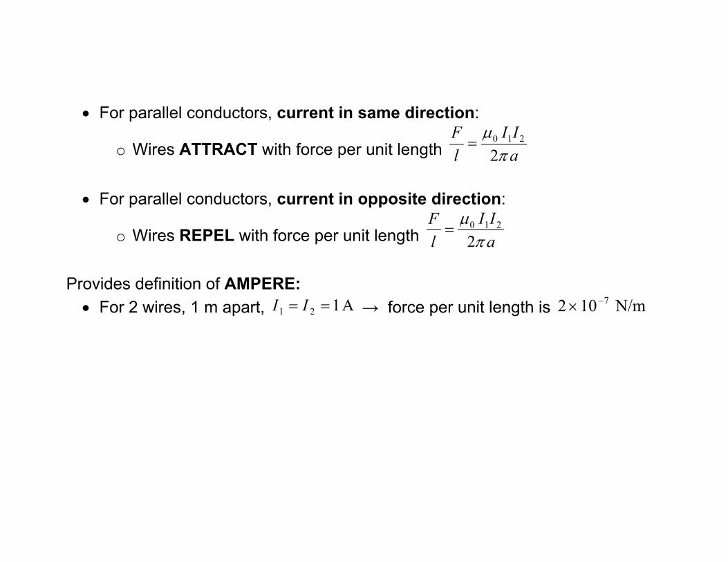
• For parallel conductors, current in same direction:
o Wires ATTRACT with force per unit length aII
lF
πµ2
210=
• For parallel conductors, current in opposite direction:
o Wires REPEL with force per unit length aII
lF
πµ2
210=
Provides definition of AMPERE: • For 2 wires, 1 m apart, A 121 == II → force per unit length is N/m 102 7−×


![The Relativistic Electron Density [1ex] and Electron ... · PDF fileThe Relativistic Electron Density and Electron Correlation Markus Reiher ... Electron density distributions for](https://img.dokumen.tips/doc/110x75/5ab2020e7f8b9aea528d15ec/the-relativistic-electron-density-1ex-and-electron-relativistic-electron-density.jpg)