Review of the API RP 14E erosional velocity equation ... Fazlollah Madani Sani.… · ©2019 by NACE International. Requests for permission to publish this manuscript in any form,

©2019 by NACE International.

Requests for permission to publish this manuscript in any form, in part or in whole, must be in writing to

NACE International, Publication Division, 15835 Park Ten Place, Houston, Texas 77084. The material presented and the views expressed in this paper are solely those of the author(s) and are not necessarily endorsed by the Association

1

Review of the API RP 14E erosional velocity equation: origin, applications, misuses and limitations

Fazlollah Madani Sani, Srdjan Nesic Institute for Corrosion and Multiphase

Technology, Ohio University 342 W State Street

Athens, Ohio, 45701 USA

Khlefa Esaklul

Occidental Petroleum Corporation 5 Greenway Plaza Suite 110

Houston, Texas, 77046 USA

Sytze Huizinga Sytze Corrosion Consultancy

Medemblikhof 39 6843 BV Arnhem The Netherlands

ABSTRACT Oil and gas companies apply different methods to limit erosion-corrosion of mild steel lines and equipment during the production of hydrocarbons from underground reservoirs. One of the frequently used methods is limiting the flow velocity to a so-called “erosional velocity,” under which it is assumed that no erosion-corrosion would occur. Over the last 40 years, the American Petroleum Institute recommended practice 14E (API RP 14E) equation has been used by many operators to estimate the erosional velocity. The API RP 14E equation has become popular because it is simple to apply and requires little in the way of inputs. However, due to its simplicity the API RP 14E equation has been frequently misused through generalizing the observed empirical 𝑐-factors to conditions and applications where it was invalid. Even when constrained to its defined conditions and applications, the API RP 14E has some serious limitations; such as not providing any quantitative guidelines for estimating the erosional velocity in the two commonest scenarios in the field, when solid particles are present in the production fluids and when erosion and corrosion are both involved. Field data showed that the API RP 14E equation is inadequate for estimating the erosional velocity and other operating parameters involved in erosion, corrosion and erosion-corrosion such as material properties, flow geometry, flow regime, sand production rate, and concentration of corrosive species; all need to be accounted for in establishing a correct estimation of the erosional velocity. Key words: API RP 14E, erosional velocity, velocity limit, erosion, erosion-corrosion, sand erosion




2

INTRODUCTION Erosion of carbon steel piping and equipment is a major problem during the production of hydrocarbons from underground reservoirs. It becomes even more complicated when electrochemical corrosion is involved. Operators continuously dig deeper in the reservoirs or use proppants and reservoir fracturing techniques in order to maintain production rates. Thus, deeper aquifers are encountered, water cuts are increased, more multiphase streams are produced, and more solids and corrosive species are introduced into the production, transportation and processing systems, which in turn leads to increased erosion-corrosion problems.1–4 The terms erosion and erosion-corrosion are often not distinguished properly. For clarity, erosion is defined as pure mechanical removal of the base metal, usually due to impingement by solid particles, although liquid droplets impingement can cause the same type of damage. Corrosion is considered to be an (electro)chemical mode of metal loss, where iron dissolves in an aqueous solution, a process that can be enhanced by intense turbulent flow. Erosion-corrosion is a combined chemo-mechanical mode of attack where both erosion and corrosion are involved. The resulting erosion-corrosion rate can be larger than the sum of erosion and corrosion rates, due to synergistic effects.5,6 Oil and gas companies have always tried to develop proper methods to limit erosion-corrosion to an acceptable level.1 One of the commonly used methods is reducing the flow velocity to a so-called “erosional velocity”, where it is thought that no erosion-corrosion would occur below this velocity.1,7 However, there have been concerns all the time about the accuracy of methods used for estimating the erosional velocity. When the estimated erosional velocity is overly conservative (low), the companies unjustifiably lose production; when it is too optimistic (high) then they risk erosion-corrosion damage and loss of system integrity. One of the method that has been extensively used over the last 40 years for estimating the erosional velocity is a recommended practice proposed by the American Petroleum Institute(1) called API RP 14E.1,8,9 The API RP 14E was originally developed for sizing of new piping systems on production platforms located offshore that carry single or two-phase flow.10 Overtime, the application of the API RP 14E mostly shifted to estimation of the erosional velocity, so that the API RP 14E is typically acknowledged as the “API RP 14E erosional velocity equation” in the field of oil and gas production. The widespread use of the API RP 14E erosional velocity equation is a result of it being simple to apply and requiring little in the way of inputs.11,12 However, it is often quoted that the API RP 14E erosional velocity equation is overly conservative and frequently unjustifiably restricts the production rate or overestimates pipe sizes.13–15 The present work provides a review of literature on the origins of the API RP 14E erosional velocity equation, its applications, misuses, and limitations.

Summary of API RP 14E The API RP 14E provides minimum requirements and guidelines for design and installation of new piping systems on production platforms located offshore. The API RP 14E offers sizing criteria for platform piping lines across three categories based on flow regime: single-phase liquid, single-phase gas and two-phase gas/liquid. The API RP 14E sizing criteria for each category are discussed below. Single-phase liquid flow lines The primary basis for sizing single-phase liquid lines is flow velocity and pressure drop. It is recommended that the pressure should always be above the vapor pressure of liquid at the given

(1) American Petroleum Institute (API), 1220 L St., N.W., Washington, DC 20005-4070.




3

temperature, in order to avoid cavitation that could lead to erosion. On the other hand, it is suggested that the velocity should not be less than 3 ft/s to minimize deposition of sand and other solids10, what presumably may lead to underdeposit corrosion attack. No other limiting criteria for determining flow velocity are mentioned that are related to erosion or erosion-corrosion. Single-phase gas flow lines For single-phase gas lines, pressure drop is the primary basis for sizing. Only a passing reference is made to a velocity limitation related to “stripping a corrosion inhibitor film from the pipe wall,” which clearly points towards erosion-corrosion.10 However, no specific guidance is offered on how to determine this limitation. Gas/liquid two-phase lines The API RP 14E lists erosional velocity, minimum velocity and pressure drop as criteria for sizing gas/liquid two-phase lines. In the appendix A of the API RP 14E two other criteria are also mentioned for sizing flow line piping: noise and pressure containment. The guideline states that “Flow lines, production manifolds, process headers and other lines transporting gas and liquid in two-phase flow should be sized primarily based on flow velocity.” On this basis, the API RP 14E recommends that when no other specific information as to erosive or corrosive properties of the fluid is available, the mixture velocity should be kept below the so-called “erosional velocity” obtained from the following empirical equation:10

𝑉𝑒 =𝑐

√𝜌𝑚

(1)

where 𝑉𝑒 is fluid erosional velocity in ft/s, 𝑐 is empirical constant in √(lb/(ft∙s2 )) (multiply by 1.21 for SI

units) and 𝜌m is gas/liquid mixture density at flowing pressure and temperature in lb/ft3. For two-phase flow, the API RP 14E states that “for solid-free fluids values of 𝑐 = 100 for continuous service and 𝑐 = 125

for intermittent service are conservative,” i.e. higher 𝑐-factors may be used. Although it is not clearly specified in the API RP 14E, this condition could be referred to a situation where corrosion is involved. For non-corrosive fluids or when corrosion is controlled by inhibition or when corrosion resistant alloys are used, the API RP 14E recommends a higher 𝑐-factor of 150 to 200 for continuous service and up to 250 for intermittent service.10 This obviously refers to situations where only mechanical erosion of the metal is of concern, and the name “erosional velocity criterion” is actually appropriate. However, it is difficult to imagine a situation where two-phase flow (without sold particles) can lead to pure mechanical erosion of the base metal without corrosion being involved. One speculation could be the mechanical removal of organic corrosion inhibitors adsorbed on the steel surface. However this is a largely controversial subject where not justifiable guidance can be offered.16 The API RP 14E further instructs that when solid production is expected, fluid velocities should be significantly reduced; however, it does not offer any specific guidance, even though this is the most critical scenario. Instead, the API RP 14E suggests that suitable 𝑐-factors need to be found from “specific application studies,” i.e. through customized testing. Finally the API RP 14E recommends what seems to be an insurance policy that in conditions under which solids are present, or corrosion is a concern or 𝑐-factors higher than 100 for continuous service are somehow used –practically cover all imaginable scenarios– periodic surveys are required in order to assess pipe wall thickness.10 In this statement, a mixture of erosion and erosion-corrosion scenarios is mentioned by the API RP 14E, which they are not

distinguishable at all. Table 1 summarizes the 𝑐-factors suggested by the API RP 14E for different conditions.




4

Table 1: Suggested 𝒄-factors by the API RP 14E for Eq. (1)10

Fluid Suggested 𝑐-factor

Continuous service Intermittent service

Solids-free

Non-corrosive Corrosive + inhibitor Corrosive + CRA*

150-200 250

Corrosive? 100 125

With solids Determine from specific application studies * Corrosion resistant alloy ? It is not exactly specified in the API RP 14E and it is the authors’ understanding

The API RP 14E erosional velocity equation needs only one input: the gas/liquid mixture density (𝜌𝑚),

which makes it easy to use. The API RP 14E suggests that 𝜌𝑚 can be calculated using the following equation:10

𝜌𝑚 = 12409𝑆𝑙𝑃 + 2.7𝑅𝑆𝑔𝑃

198.7𝑃 + 𝑅𝑇Ƶ (2)

where 𝑃 is operating pressure in psia, 𝑆𝑙 is liquid specific gravity at standard conditions (water = 1), 𝑆𝑔 is

gas specific gravity at standard conditions (air = 1), 𝑅 is gas/liquid ratio at standard conditions, 𝑇 is operating temperature in Rankine scale (oR) and Ƶ is gas compressibility factor. Once the erosional

velocity (𝑉𝑒) is determined, the minimum cross-sectional area required to avoid erosion can be calculated using the following equation:10

𝐴 = 9.35 +

𝑅𝑇Ƶ21.25𝑃

𝑉𝑒 (3)

where 𝐴 is minimum pipe cross-sectional flow area required in in2/1000 barrels liquid per day. While the API RP 14E presents a simple erosional velocity criterion, as expressed by Eq. (1), it is not clear at all clear how such a simple expression, with only one adjustable constant, can cover a broad array of scenarios seen across different two-phase gas/liquid flow regimes (stratified, slug, annular-mist, bubble, churn, etc.), with and without solids, in the presence or absence of corrosion, with and without inhibition, for mild steel as well as CRAs. The differences in erosion and erosion-corrosion mechanisms are so large that it seems next to impossible to capture all the possible scenarios with one such simple expression. However, before jumping to any conclusion, the origin of this empirical equation should be examined because it may form a rationale for its use.

Origin of API RP 14E erosional velocity equation The API RP 14E was first published in 1978. Ever since, its origin has been the subject of much debate in the open literature. The oldest reference found proposing an equation similar to the API RP 14E equation is the Coulson and Richardson’s Chemical Engineering book from 1979.17 It suggests the following empirical equation to obtain the velocity at which erosion becomes significant:

𝜌𝑀𝑢𝑀2 = 15,000 (4)




5

where 𝜌𝑀 is the mean density of two-phase mixture in kg/m3 and 𝑢M is the mean velocity of two-phase

mixture in m/s. When Eq. (4) is solved for 𝑢𝑀 the same expression as the API RP 14 equation will be obtained with a 𝑐-factor of 122 (in SI units), which is equivalent to a 𝑐-factor of 100 in the imperial units. However, there is no information in the book about the origin of Eq. (4) either. It can be speculated that Eq. (4) represents some sort of an energy balance, with the left side representing kinetic energy of the flow (probably liquid droplets) and the right side being the amount of energy required to cause erosion. A qualitatively similar argument was presented later by Lotz and Badhuisweg.18 In 1983, Salama and Venkatesh2 speculated that the API RP 14E equation might not be a pure empirical equation and suggested one of the following three approaches could be its origin: (1) Bernoulli equation with a constant pressure drop

Solving the Bernoulli equation for velocity (𝑉) with the assumptions of no gravity effects and an initial velocity of zero results in Eq. (5), which has a similar form as the API RP 14E equation.

𝑉 = √2∆𝑃

√𝜌 (5)

where 𝑉 is the fluid velocity in ft/s, ∆𝑃 is the total pressure drop along the flow path in psi, and

𝜌 is the fluid density in lb/ft3. Salama and Venkatesh2 claimed that a typical total pressure drop for high capacity wells is between 3000 and 5000 psi. Plugging these numbers into Eq. (5) results in a 𝑐-factor in the range of 77 to 100. They concluded that although Eq. (5) and the API RP 14E equation seem to be similar, “they should have no correlation because they represent two completely different phenomena.”2 Indeed, it is difficult to imagine how the Bernoulli equation can be connected to erosion of a metal, without introducing speculative assumptions along the way. One such hypothetical scenario would be flow of a fluid through a sudden constriction, such as a valve, which would cause sudden acceleration of the fluid and an associated pressure drop that can be estimated by using Eq. (5).19 If the total pressure of the system falls below the vapor pressure of the liquid, cavitation could happen that leads to metal erosion. (2) Erosion due to liquid impingement In another attempt to justify the origin of the API RP 14E equation, Salama and Venkatesh2 used the following equation, which they attributed to Griffith and Rabinowicz, for calculating erosion due to liquid impingement:

ℎ =𝐾𝜈𝜌𝑉2

2𝑃𝑔 (

2

27

𝜌𝑉2

𝑔𝑃𝜖𝑐2)

21

𝐴 (6)

where ℎ is penetration rate in mpy, 𝐾 is high-speed erosion coefficient (≅0.01), 𝜈 is impacting fluid volume rate in ft3/s (𝜈 =𝐴𝑉), 𝜌 is fluid density in lb/ft3, 𝑉 is impact velocity of the fluid in ft/s, 𝑃 is target material hardness in psi (= 1.55105 psi for steel), 𝑔 is gravitational constant (32.2 ft/s2), 𝜖𝑐 is critical strain to failure (0.1 for steel) and 𝐴 is cross-sectional area of pipe in ft2. By making a number of arbitrary assumptions, Salama and Venkatesh2 were apparently able to reduce this equation to a form similar to the API RP 14E equation:

𝑉 ≅300

√𝜌 (7)

where 𝑉 and 𝜌 are the same as those in Eq. (6). For more details on the simplification procedure, the reader is referred to the original paper. Eq. (7) is similar in form to the API RP 14E equation with a




6

corresponding 𝑐-factor of 300. However, it was not possible for the authors to reproduce this derivation

and recover the same 𝑐-factor, as it seems there was an inconsistency in the units in the original publication.2 Craig20 altered Salama and Venkatesh’s approach by using the same equation as Eq. (6) with a high

speed coefficient (𝐾) of 10-5 and units of ft/s for penetration rate (ℎ) and psf for target material hardness (𝑃). Craig20 proposed that liquid droplet impingement causes damage by removing the corrosion product film from the surface and not removing the base metal itself. Thus, he substituted the values of 𝑃 and the

critical failure strain (𝜖𝑐) for steel (used by Salama and Venkatesh) with those for magnetite (Fe3O4) (𝑃 = 1.23×108 psf and 𝜖𝑐 = 0.003) in Eq. (6). He simplified Eq. (6) to obtain the following equation by considering a penetration rate of 10-11 ft/s:

𝑉 =150

√𝜌37 (8)

where 𝑉 and 𝜌 are the same as those in Eq. (6). Using an argument similar to Craig, Smart21 stated that the API RP 14E equation represents velocities needed to remove a corrosion product films by “droplet impingement fatigue,” as the flow regime in multiphase systems transits to annular mist flow (presumably as erosion-corrosion scenario). However, Arabnejad et al.22 showed that the trend of the erosional velocity calculated by the API RP 14E equation did not correlate well with empirical data on erosion-corrosion caused by liquid droplet impingement. Deffenbaugh et al.23 suggested that 400 ft/s is the approximate droplet impingement erosional velocity. The DNV GL recommended practice O501 suggests a threshold velocity of 230-262 ft/s to avoid droplet impingement erosion in gas-condensate systems.24

If these velocities are plugged into the API RP 14E equation with a 𝑐-factor ranging from 100 to 300, the resulting mixture density falls between 0.06 to 1.7 lb/ft3, which is extremely low for a gas/liquid two-phase flow, making the linkage between the API RP 14E equation and liquid impingement implausible. Moreover, typical fluid velocities seen in oil and gas piping applications are far below the abovementioned droplet impingement erosional velocities, casting doubts that liquid droplet impingement can be considered as a reasonable erosional mechanism behind the API RP 14E equation.23 (3) Removal of corrosion inhibitor films As their last attempt, Salama and Venkatesh2 assumed that the API RP 14E equation presents a velocity above which the flow could remove a protective corrosion inhibitor film from the surface of steel tubulars (a possible erosion-corrosion scenario). According to Salama and Venkatesh2, the erosional velocity can be calculated from the following equation:

𝑉 =√

8𝑔𝜏𝑓

√𝜌

(9)

where 𝑉 is the velocity to remove the corrosion inhibitor film from the surface in ft/s, 𝑔 is the gravitational constant (32.2 ft/s2), 𝜏 is the shear strength of the inhibitor interface in psi, 𝑓 is the friction factor and 𝜌 is the fluid density in lb/ft3. Eq. (9) is apparently obtained by setting the flow-induced wall shear stress equal to the shear strength (𝜏) of the inhibitor film. However, Eq. (9) is not consistent when it comes to the units, i.e. the gravitational constant (𝑔) does not fit into the equation. Despite this, Salama and Venkatesh2

simplified Eq. (9) by considering 𝜏 equals 8000 psi and 𝑓 equals 0.0015 and derived an equation similar to the API RP 14E equation:

𝑉 =35,000

√𝜌 (10)




7

where 𝑉 and 𝜌 are the same as those in Eq. (9). Craig20 mentioned that 𝑓 = 0.0015 is meant for smooth pipes and a value of 0.03 is more consistent with scale-roughened surfaces. In addition, Craig20 used psf

unit instead of psi for 𝜏 in Eq. (9), resulting in a constant value of approximately 100,000. Either way, Eq. (10) has the same form as the API RP 14E equation; however, the constants found by Salama and

Venkatesh2, and Craig20 were much larger than the 𝑐-factors considered for the API RP 14E equation, leading to very high erosional velocities, orders of magnitude higher than those seen in oil and gas wells. Even if the error in the units is ignored, it seems that the removal of corrosion inhibitor film could not have been used as a background for deriving the API RP 14E equation. Finally, quite a few researchers simply stated that the API RP 14E equation has no theoretical justification and it is a pure empirical equation. For example, Smart25 stated that the API RP 14E equation was apparently obtained from Keeth’s report26 on erosion-corrosion problems encountered in steam power plants, where multiphase steam-condensate piping systems were used. However, no information on velocity limitation could be found in this report.26–28 Castle et al.29 believed that the API RP 14E equation was formulated based on the field experience with wells in the Gulf Coast area, as a criterion for the maximum velocity in carbon steel piping needed to avoid the removal of protective inhibitor films or corrosion products (an erosion-corrosion scenario). Heidersbach30 suggested that the API RP 14E equation was adapted from a petroleum refinery practice in which the flow velocity was kept below the API RP 14E erosional velocity to minimize pumping requirements that become prohibitively expensive at

high flow velocities. Salama27 cited Gipson who mentioned that the proposed 𝑐-factor in the API RP 14E equation is to prevent excessive noise in a piping system. Wood31 stated that the origin of the API RP 14E equation was from US Naval steam pipe specifications. Patton32 reported that the API RP 14E equation was developed by the US Navy during World War II with a 𝑐-factor of 160 for carbon steel piping in solid-free fluids. Subsequently, the 𝑐-factor was changed to 100 when the equation was incorporated

by the API. Another anecdote is that similar equations to the API RP 14E equation with 𝑐-factors ranging from 80 to 160 had been used in various oil companies before the API committee members wrote the API 14E recommended practice.25 Clearly, none of the abovementioned theoretical explanations (energy balance, Bernoulli equation, liquid impingement, corrosion inhibitor/product removal) that supposedly underpin the API RP 14E equation seem to properly justify its form. The alternative explanations involving anecdotal evidence are even less convincing. Subscribing to any of the above explanations about the origin of the API RP 14E does not change the fact that the API RP 14E equation has been used widely in the oil and gas industry, albeit with varying degrees of success. Therefore, it is worthwhile reviewing some of the publicized applications of the API RP 14E equation, followed by its misuses and limitations.

Some applications of API RP 14E erosional velocity equation Although the origin and even the validity of the API RP 14E equation has been questioned by many, its application within the oil and gas industry has been widespread. The following are a few examples of the application of the API RP 14E equation in the oil and gas industry. According to Smart25, the first application of the API RP 14E equation was in the corrosive gas-condensate fields of Gulf of Mexico. Deffenbaugh and Buckingham23 reported that Atlantic Richfield Company (ARCO) considered the API RP 14E equation as overly conservative for straight tubing with non-corrosive solid-free fluids. ARCO recommended a 𝑐-factor of 150 for continuous service and a 𝑐-factor of 250 for intermittent service when corrosion is prevented or controlled by dehydrating the fluids, using corrosion inhibitors or employing CRAs.23 It is not entirely clear in this scenario how metal loss happens at all, when there are no solid particles in the flow stream, neither is there any corrosion, and




8

therefore from a mechanistic point of view it is difficult to justify these 𝑐-factors and the associated velocity limits. Salama9 has quoted Erichsen who reported data from a condensate field in the North Sea operating with a 𝑐-factor of 726 (equivalent to a flow velocity of 286 ft/s) for 3 years until a failure occurred in AISI 4140 carbon steel tubing at the flow coupling, which was attributed to liquid droplet impingement. Another operator in North Sea chose a 𝑐-factor of 300 as the upper limit for Gullfaks subsea water injectors completed with API L80 13Cr tubing. Chevron produced from a gas-condensate reservoir in North West Shelf of Western Australia with pressure of 4500 psi and temperature of 110oC at a velocity just below the wellhead of 121 ft/s (corresponded to a 𝑐-factor of 400 ) in 7” OD tubing and at 59 ft/s (corresponded to a 𝑐-factor of 200) in 9 5/8” OD tubing with no failure.33 At North Rankin offshore gas field in the North West region of Western Australia, velocities up to 98 ft/s, three times the API erosional velocity were used in carbon steel tubing over long periods of production without any sign of erosion.29 In a case study done by the National Iranian Oil Company on four gas wells in Parsian gas-condensate field in southern Iran, 𝑐-factors in the range of 149 (velocity of 55 ft/s) to 195 (velocity of 74 ft/s) caused

no unexpected erosion damage. Therefore, the operator suggested to use an average 𝑐-factor of 170 as a safe value for all those wells.12 In a similar research conducted in South Pars gas field in southern Iran

on four gas-condensate wells, it was reported that 𝑐-factors in the range of 138 to 193 were safe for production.34 BP Amoco limited the velocities in production from gas wells in Endicott field, Alaska North Slope to approximately 3 times the API erosional velocity based on an experience that fluids with very small amount of entrained solids flowing through SS pipelines caused minimal risk of erosion at those velocities.35 Before 1993, Shell used a modified version of the API RP 14E equation with a 𝑐-factor of 160 for sand-free service, 120 for moderate-sand service and 80 for severe-sand services. Since 1993 and before switching to a modified version of the Tulsa Model36, Shell stopped using the API RP 14E equation and set the limiting erosional velocity directly according to the type of failure mechanism, and verified that velocity with appropriate monitoring and inspection.37 It is quite possible that the above practices no longer reflect the current practices being used in the mentioned companies.23 Even then, in almost all the reported field cases, 𝑐-factors higher than those suggested by the API RP 14E were used, with a very large spread.

Misuses of API RP 14E erosional velocity equation The API RP 14E equation is intended for use in flow lines, production manifolds, process headers and other lines transporting gas and liquid two-phase fluids on production platforms located offshore. The API RP 14E clearly states a specific range of 𝑐-factors for “solid-free fluids where corrosion is not anticipated or when corrosion is controlled by inhibition or by employing corrosion resistant alloys.” These conditions are commonly recognized as “clean” service. Presumably, for solid-free corrosive fluids the API RP 14E

equation can also be used with a 𝑐-factor of 100, although it is considered conservative. In the presence of solids, reduced 𝑐-factors are recommended if “specific application studies have shown them to be appropriate.” However, no explicit guideline is provided by the API RP 14E.10 Obviously, in conditions




9

other than those mentioned above, the API RP 14E equation should not be used, at least not without special justification. However, probably due to lack of alternatives, the API RP 14E equation has been used widely with arbitrary choice of 𝑐-factors for a variety of conditions such as single-phase flow service, uninhibited corrosive systems with a corrosion product film as well as for flow containing solids.9,28 Another problematic use of the API RP 14E equation was for sizing downhole tubulars, which were not included in the original recommended practice.8,25,30 The recommended steel grade for downhole tubulars is API 5A which is generally harder and stronger than API 5L steel grade recommended the by API RP 14E.30 Therefore, if applicable at all, the original API RP 14E erosional velocity would be conservative for downhole tubulars. The lack of generality of the API RP 14E equation was clearly recognized in the past, and some attempts

were made to improve its performance by presenting functions for calculation of the 𝑐-factor. However, this just compounded the problem where an empirical equation —already performed inadequately and could not be extrapolated across different conditions— was altered by making it even more complex, without proper justification. In the most general sense, the misuse of the API RP 14E equation stems from its doubtful origin and the fact that it has been used in all kinds of conditions and applications for which it was not intended for. This is based on a problematic assumption (often implicit) that the API RP 14E equation can be used as means of generalizing observed empirical erosion, flow-affected corrosion (FAC) or erosion-corrosion data to derive safe operational velocities for a broad variety of conditions (usually fall outside the experimental range). This assumption ignores the fact that the mechanism and the rate of degradation can be very different (by orders of magnitude) depending on type of service or even within the same type of service. Thus, the API RP 14E equation cannot be simply used in different conditions by just modifying the 𝑐-factor, assuming that it is universally valid and it will give reasonable values. Even if the use of the API RP 14E equation is narrowed down to applications for which it was originally proposed and the API RP 14E equation is assumed to be fundamentally correct, which seems to be a stretch, it has some limitations that are presented in the following section.

Limitations of API RP 14E erosional velocity equation The API RP 14E equation while offering a simple approach to calculate the erosional velocity, has some serious limitations:8

The equation only considers the density of fluid in calculating the erosional velocity, while many other influential factors such as pipe material, fluid properties, flow geometry and flow regime are not accounted.8,38,39

In calculation of the mixture density in the API RP 14E equation, it is assumed that there is no slip between gas and liquid and that both phases flow at a same velocity in the pipe. However, in many flow regimes, such as stratified flow, the gas and liquid velocities are not equal (there is slip between the two phases), and the liquid moves much slower than the gas. Therefore, the actual mixture density at any discrete location in the pipe can be considerably different from the no-slip mixture density.38

The API RP 14E equation suggests that the limiting erosional velocity increases when the fluid density decreases. This does not agree with experimental observations for liquid droplet impingement and sand erosion in which the erosion is higher in low-density fluids.2,8 In high-density fluids, most of the solid particles are carried in the center of the flow stream without significantly impacting the surface2.




10

Moreover, the presence of a high-density fluid cushions the impact of solid particles or droplets at the pipe wall, so that the limiting erosional velocity actually increases.7

The API RP 14E equation only considers flow lines, production manifolds and process headers, treating them all in the same way in terms of limiting the velocity. However, areas with flow disturbances such as chokes, elbows, long radius bends, tees, etc., where most of the erosion/corrosion problems occur are not differentiated by the equation.38,40

The API RP 14E equation does not offer any guideline on how to estimate the erosion rate, neither below nor above the limiting erosional velocity. It also does not specify a generally allowable amount of erosion, in terms of rate of wall thickness loss (e.g. 5 to 10 mpy).8

Probably the most significant limitation of the API RP 14E equation is that it does not provide any quantitative guidelines for estimating the erosional velocity when solid particles are present in the

production fluid (erosion) or when both are an issue (erosion-corrosion), assuming that 𝑐 = 100 is defined for corrosive conditions.

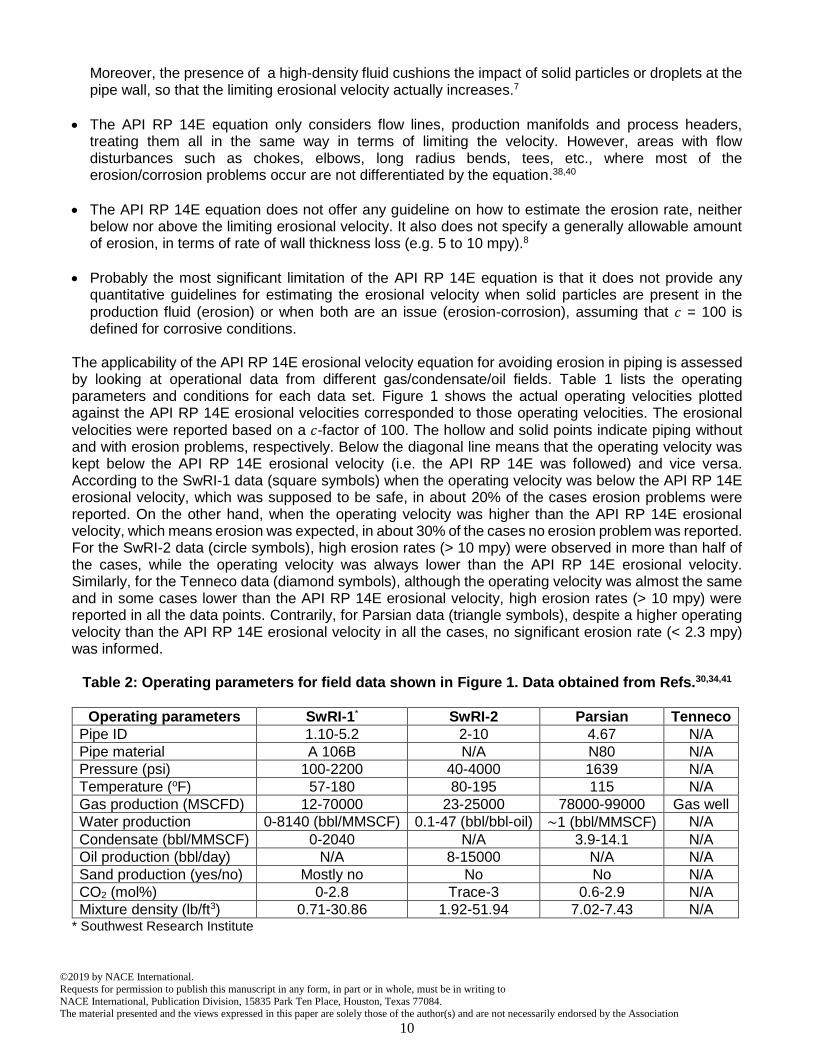
The applicability of the API RP 14E erosional velocity equation for avoiding erosion in piping is assessed by looking at operational data from different gas/condensate/oil fields. Table 1 lists the operating parameters and conditions for each data set. Figure 1 shows the actual operating velocities plotted against the API RP 14E erosional velocities corresponded to those operating velocities. The erosional

velocities were reported based on a 𝑐-factor of 100. The hollow and solid points indicate piping without and with erosion problems, respectively. Below the diagonal line means that the operating velocity was kept below the API RP 14E erosional velocity (i.e. the API RP 14E was followed) and vice versa. According to the SwRI-1 data (square symbols) when the operating velocity was below the API RP 14E erosional velocity, which was supposed to be safe, in about 20% of the cases erosion problems were reported. On the other hand, when the operating velocity was higher than the API RP 14E erosional velocity, which means erosion was expected, in about 30% of the cases no erosion problem was reported. For the SwRI-2 data (circle symbols), high erosion rates (> 10 mpy) were observed in more than half of the cases, while the operating velocity was always lower than the API RP 14E erosional velocity. Similarly, for the Tenneco data (diamond symbols), although the operating velocity was almost the same and in some cases lower than the API RP 14E erosional velocity, high erosion rates (> 10 mpy) were reported in all the data points. Contrarily, for Parsian data (triangle symbols), despite a higher operating velocity than the API RP 14E erosional velocity in all the cases, no significant erosion rate (< 2.3 mpy) was informed.

Table 2: Operating parameters for field data shown in Figure 1. Data obtained from Refs.30,34,41

Operating parameters SwRI-1* SwRI-2 Parsian Tenneco

Pipe ID 1.10-5.2 2-10 4.67 N/A

Pipe material A 106B N/A N80 N/A

Pressure (psi) 100-2200 40-4000 1639 N/A

Temperature (oF) 57-180 80-195 115 N/A

Gas production (MSCFD) 12-70000 23-25000 78000-99000 Gas well

Water production 0-8140 (bbl/MMSCF) 0.1-47 (bbl/bbl-oil) ~1 (bbl/MMSCF) N/A

Condensate (bbl/MMSCF) 0-2040 N/A 3.9-14.1 N/A

Oil production (bbl/day) N/A 8-15000 N/A N/A

Sand production (yes/no) Mostly no No No N/A

CO2 (mol%) 0-2.8 Trace-3 0.6-2.9 N/A

Mixture density (lb/ft3) 0.71-30.86 1.92-51.94 7.02-7.43 N/A * Southwest Research Institute




11

Figure 2 shows the empirical erosion rate data as a function of equivalent API RP 14E 𝑐-factor, which was calculated by substituting the actual operating velocity and its corresponding mixture velocity into Eq. (1). The operating conditions for Tabnak, Shanoul, Kangan, and Varavy gas fields (in southern Iran) were similar to Parsian gas field shown in Table 1. It is assumed that an erosion rate of 5 mpy is the maximum allowable erosion rate. The SwRI-2 data show that even though the equivalent 𝑐-factor was

sufficiently below 100 (the recommended 𝑐-factor by API RP 14E), the erosion rate was significantly higher than 5 mpy in approximately 60% of the cases. Oppositely, for the four gas fields despite equivalent 𝑐-factors higher than 100, the erosion rates were negligible. Jordan37 by using SwRI data showed that for two-phase flows with high liquid velocities, the estimated erosional velocity by the API RP 14E equation is conservative (high). However, for two-phase flows with low liquid and high gas velocities the estimated erosional velocity can be risky (low). Therefore, it can be concluded that the API RP 14E erosional velocity criterion underpredicted the erosional velocity in some cases (risky) and overpredicted that in some other cases (conservative). Therefore, the API RP 14E erosional velocity equation is not adequate for estimating the erosional velocity and other operating parameters such as material properties, flow geometry, flow regime, sand production rate, and concentration of corrosive species need to be accounted for a correct estimation of the erosional velocity.

Figure 1: Operating velocity vs. corresponding API RP 14E erosional velocity. Data are borrowed from Refs.30,34,41




12

Figure 2: Empirical average erosion rate vs. corresponding equivalent API RP 14E 𝒄-factor; 5 mpy is assumed to be the maximum allowable erosion rate; data are taken from Refs.34,41

Recommendation The following iterative procedure in Figure 3 is recommended for estimating the erosional velocity in erosive/corrosive service based on a model proposed by Al-Mutahar et al.42:

Define an allowable material loss rate for the system (e.g. 5 mpy).

Choose a superficial liquid velocity (Vsl) and a superficial gas velocity (Vsg) starting from low values (the average fluid velocity (V0) is assumed to be the summation of Vsl and Vsg)

Estimate the formation rate of corrosion product film (FRCP) on the surface by using a thermodynamic/corrosion prediction software such as MULTICORP™, OLI Systems or Thermo-Calc.

Estimate the erosion rate of the bare metal (ER) and the corrosion product film (ERCP) by using an erosion model such as the Tulsa model (SPPS software) or the DNV GL model (Pipeng Toolbox). For ERCP, the target material in the erosion models should be the corrosion product film. For example, in CO2 environments, the iron carbonate (FeCO3), which its hardness is around 240 Brinell, should be considered as the target material in the erosion models.

If a corrosion product film does not form on the surface (thermodynamically unfavorable) or the formation rate of the corrosion product film is smaller than its erosion rate (ERCP) (the film does not remain on the surface because of erosion), the total erosion-corrosion rate is assumed to be the summation of the erosion rate (ER) and the corrosion rate (CR).

If the formation rate of the corrosion product film is greater than its erosion rate (ERCP), increase the scale thickness (e.g. h) in the corrosion prediction software (increments of (∆h)) until the formation rate of the corrosion product film and its erosion rate become equal. At this stage (steady state), it is assumed that the erosion rate (ERCP) is zero and the total erosion-corrosion rate is equal to the corrosion rate of the bare metal covered with a corrosion product film (thickness of hsteady state) (CRCP).




13

If the predicted erosion-corrosion rate is equal to the defined allowable material loss, the chosen V0 is the erosional velocity limit, otherwise, iterate the above steps with a higher Vsg and Vsl.

Figure 3: The flowchart for estimating the erosional velocity, considering both erosion and

corrosion (based on a model by Al-Mutahar et al.42)

Conclusion

The widespread use of the API RP 14E erosional velocity equation is due to its simplicity in terms of required inputs.11,12 However, the API RP 14E equation does not account for most of the key parameters involved in erosion, corrosion and erosion-corrosion.

The origin of the API RP 14E erosional velocity equation remains unclear. The theoretical explanations (e.g., energy balance, Bernoulli equation, liquid droplet impingement, and corrosion inhibitor/product removal) that supposedly underpin the API RP 14E equation do not seem to properly justify its form. Alternative explanations involving anecdotal evidence on empirical origins of the API RP 14E equation are even less convincing.

Despite its widespread use, the API RP 14E equation has many limitations. Probably the most critical one is that it does not provide any quantitative guidelines for estimating the erosional velocity in the two most seen scenarios in the field: when solid particles are present in the production fluids (erosion) or when erosion and corrosion are both an issue (erosion-corrosion),

assuming that 𝑐 = 100 is defined for corrosive conditions (corrosion). A reduction in the 𝑐-factor is recommended for these scenarios, although it is unclear how to obtain its exact value.

When the API RP 14E equation is used for two-phase flows with high liquid velocities (Vsl), the estimated erosional velocity will be conservative (high). However, for two-phase flows with low liquid and high gas velocities (Vsg) the estimated erosional velocity can be risky (low).

Data Collection

Corrosion product film

forms? Yes

No Yes

No

Yes

Needed data: component properties (material, geometry, diameter), sand properties (size, shape, density, flow rate), flow conditions

(temperature, PCO2, PH2S, pH, [Fe2+

], ionic strength), flow regime

(annular-mist, slug, stratified, bubbly, etc.)

E/CR = ER + CR

Estimate erosion rate of bare metal (ER)

and corrosion product film (ERCP)

Estimate formation rate of corrosion

product film (FRCP)

Erosion prediction models such as Tulsa or DNV GL models. For ERCP, the

target material used in the models should be the corrosion product film. FeCO3 hardness ~ 240 Brinell

Corrosion prediction software such as MULTICORP™, OLI Systems and Thermo-Calc. Corrosion products such as iron carbonate, iron sulfide

Add film layer (∆h) and recalculate FRCP FR

CP < ER

CP? FR

CP = ER

CP?

E/CR = CRCP

No

Choose/change Vsl and Vsg

(V0 = Vsl +Vsg)

E/CR=allowable material loss

rate? Yes

No

V0 = erosional velocity

Define an allowable material loss rate

(e.g. 5 mpy)

E/CR: total erosion-corrosion rate ER: erosion rate of bare metal CR: corrosion rate of bare metal

CRCP: corrosion rate of bare

metal covered with a corrosion product film




14

Empirical data showed that the API RP 14E erosional velocity equation is inadequate for estimating the erosional velocity and other operating parameters such as material properties, flow geometry, flow regime, sand production rate, and concentration of corrosive species need to be accounted for to establish a correct estimation of the erosional velocity.

A proper erosion-corrosion model applicable to the vast majority of conditions in oil and gas production systems, determining whether there is a feasible case for increasing the flow velocity limit, allows higher production rates, cheaper materials to be used or smaller diameter pipelines.

ACKNOWLEDGEMENTS The authors would like to gratefully acknowledge the constructive help of Dr. David Young and Dr. Hamed Mansouri (Institute for Corrosion and Multiphase Technology (ICMT)), Anthony James Bianco Jr., Patrick Andrew Kelley and Quinten Orantek (Ohio University), Mr. Kamal Pakdaman (BACO for Oil Industry Construction, Basra), and Mr. Hossein Jafari (Iranian Offshore Engineering and Construction Company) during the writing of this review paper.

REFERENCES 1. McLaury, B.S., J. Wang, S.A. Shirazi, J.R. Shadley, and E.F. Rybicki, “Solid Particle Erosion in Long

Radius Elbows and Straight Pipes” (Society of Petroleum Engineers, 1997). 2. Salama, M.M., and E.S. Venkatesh, “Evaluation of API RP 14E Erosional Velocity Limitations for

Offshore Gas Wells” (OnePetro, 1983). 3. Arabnejad, H., A. Mansouri, S.A. Shirazi, and B.S. McLaury, Wear 376–377, Part B (2017): pp.

1194–1199. 4. Lusk, D., M. Gupta, and K. Boinapally, “Armoured against Corrosion” (Hydrocarbon Engineering,

2008). 5. Wood, R.J.K., and S.P. Hutton, Wear 140 (1990): pp. 387–394. 6. Malka, R., S. Nešić, and D.A. Gulino, Wear 262 (2007): pp. 791–799. 7. Arabnejad, H., S.A. Shirazi, B.S. McLaury, and J.R. Shadley, “Calculation of Erosional Velocity Due

to Liquid Droplets with Application to Oil and Gas Industry Production” (Society of Petroleum Engineers, 2013).

8. Shirazi, S.A., B.S. McLaury, J.R. Shadley, and E.F. Rybicki, J. Pet. Technol. 47 (1995): pp. 693–698.

9. Salama, M.M., J. Energy Resour. Technol. 122 (2000): pp. 71–77. 10. “API RP 14E : Recommended Practice for Design and Installation of Offshore Production Platform

Piping Systems” (American Petroleum Institute, 1991). 11. McLaury, B.S., S.A. Shirazi, and E.F. Rybicki, “Sand Erosion in Multiphase Flow for Slug and

Annular Flow Regimes,” in CORROSION (San Antonio, TX: NACE International, 2010), p. No. 10377.

12. Mansoori, H., F. Esmaeilzadeh, D. Mowla, and A.H. Mohammadi, Oil Gas J. (2013). 13. Mofrad, S.R., “Erosional Velocity Limit” (2014). 14. Russell, R., S. Shirazi, and J. Macrae, “A New Computational Fluid Dynamics Model to Predict Flow

Profiles and Erosion Rates in Downhole Completion Equipment” (Society of Petroleum Engineers, 2004).

15. Arabnejad Khanouki, H., S.A. Shirazi, B.S. McLaury, and J.R. Shadley, “A Guideline to Calculate Erosional Velocity Due to Liquid Droplets for Oil and Gas Industry” (Society of Petroleum Engineers, 2014).

16. Li, W., B.F.M. Pots, X. Zhong, and S. Nesic, Corros. Sci. 126 (2017): pp. 208–226.




15

17. Coulson, J.M., and J.F. Richardson, Chemical Engineering, Vol. 1: SI Units, 3rd edition (Pergamon Press, 1977).

18. Lotz, U., “Velocity Effects in Flow Induced Corrosion,” in CORROSION (NACE International, 1990), p. No. 27.

19. Hattori, S., and M. Takinami, Wear 269 (2010): pp. 310–316. 20. Craig, B., Oil Gas J. 83 (1985): pp. 99–100. 21. Smart, J.S., “The Meaning of the API RP 14E Formula for Erosion Corrosion in Oil and Gas

Production” (Cincinnati, OH: NACE International, 1991), p. No. 468. 22. Arabnejad, H., A. Mansouri, S.A. Shirazi, B.S. McLaury, and J.R. Shadley, “Erosion-Corrosion Study

of Oil-Field Materials Due to Liquid Impact,” in CORROSION (Dallas, TX: NACE International, 2015), p. No. 6136.

23. Deffenbaugh, D.M., and J.C. Buckingham, “A Study of the Erosional Corrosional Velocity Criterion for Sizing Multi-Phase Flow Lines, Phase I” (Reston, VA: Southwest Research Institute, 1989).

24. “DNV Gl-RP-O501 Recommended Practice: Erosive Wear in Piping Systems, Revision 4.2” (Det Norske Veritas, 2011).

25. Smart, J.S., “A Review of Erosion Corrosion in Oil and Gas Production,” in CORROSION (Las Vegas, NV: NACE International, 1990), p. No. 10.

26. Keeth, J.A., Corrosion 11 (1946): pp. 101–124. 27. Salama, M.M., Mater. Perform. 32 (1993): p. 7. 28. Andrews, P., T.F. Illson, and S.J. Matthews, Wear 233–235 (1999): pp. 568–574. 29. Castle M.J., and Teng D.T., “Extending Gas Well Velocity Limits: Problems and Solutions,” in Soc.

Pet. Eng. SPE (Perth, Western Australia, 1991), pp. 135–144. 30. Heidersbach, R., “Velocity Limits for Erosion-Corrosion” (Dallas, TX, 1985). 31. Wood, R.J.K., Wear 261 (2006): pp. 1012–1023. 32. Patton, C.C., “Are We out of the Iron Age Yet?,” in CORROSION (NACE International, 1993), p. No.

93056. 33. Panic, D., and J. House, “Challenging Conventional Erosional Velocity Limitations for High Rate

Gas Wells” (2009), p. 6. 34. Ariana, M.A., F. Esmaeilzadeh, and D. Mowla, Phys. Chem. Res. 6 (2018): pp. 193–207. 35. “Annual Report to Alaska Department of Environmental Conservation: Commitment to Corrosion

Monitoring” (Corrosion, Inspection and Chemicals (CIC) Group, BP Exploration (Alaska) Inc., 2002). 36. Parsi, M., K. Najmi, F. Najafifard, S. Hassani, B.S. McLaury, and S.A. Shirazi, J. Nat. Gas Sci. Eng.

21 (2014): pp. 850–873. 37. Jordan, K., “Erosion in Multiphase Production of Oil & Gas,” in CORROSION (San Diego, California,

1998), p. No. 5834. 38. Svedeman, S.J., and K.E. Arnold, SPE Prod. Facil. 9 (1994): pp. 74–80. 39. Richard Udoh, R., “Sand and Fines in Multiphase Oil and Gas Production,” Master’s thesis,

Norwegian University of Science and Technology, 2013. 40. Salazar, A.T., “Erosional Velocity Limitations for Oil and Gas Wells - Extracted from Neotec Wellflow

Manual” (2012). 41. Svedeman, S.J., “A Study of the Erosional/Corrosional Velocity Criterion for Sizing Multiphase Flow

Lines, Phase II” (Reston, VA: Southwest Research Institute, 1990). 42. Al-Mutahar, F.M., K.P. Roberts, S.A. Shirazi, E.F. Rybicki, and J.R. Shadley, “Modeling and

Experiments of FeCO3 Scale Growth and Removal for Erosion-Corrosion Conditions,” in CORROSION (NACE International, 2012), p. No. 1132.

Documents

Review of the API RP 14E erosional velocity equation ... Fazlollah Madani Sani.… · ©2019 by NACE International. Requests for permission to publish this manuscript in any form,