Embed Size (px)
Citation preview
REVIEW OF METHODS FOR ASSESSING THE APPLICABILTY
DOMAINS OF SARS AND QSARS
PAPER 1: Review of methods for QSAR applicability domain
estimation by the training set
Author:
Dr Joanna Jaworska (Procter & Gamble, Strombeek – Bever, Belgium) E-mail: [email protected] Dr Tom Aldenberg (RIVM, Bilthoven, NL) E-mail: [email protected] Dr Nina Nikolova (Bulgarian Academy of Sciences, Sofia, Bulgaria) E-mail: [email protected] Sponsor: The European Commission - Joint Research Centre Institute for Health & Consumer Protection - ECVAM 21020 Ispra (VA) Italy Contact: Dr Andrew Worth E-mail: [email protected] http://ecb.jrc.it/QSAR JRC Contract ECVA-CCR.496575-Z
VERSION OF 28 JANUARY 2005

REVIEW OF STATISTICAL METHODS FOR QSAR AD ESTIMATION BY THE TRAINING SET
Joanna Jaworska1, Nina Nikolova-Jeliazkova2, Tom Aldenberg3
1Procter & Gamble, Eurocor, Strombeek-Bever, Belgium; 2 Institute of Parallel Processing - Bulgarian
Academy of Sciences, Sofia, Bulgaria; 3RIVM, Bilthoven, Netherlands
Address for the correspondence and reprints: Joanna Jaworska Procter & Gamble, Eurocor, Central Product
Safety, 100 Temselaan, B-1853 Strombeek – Bever, Belgium (email address: [email protected]; fax nr.
+32-2-568.3098)
1
Summary
As QSAR models use for decision making related to chemical management increases, the reliability of the
model predictions is a growing concern. One of the conditions that will assure reliable predictions by the
model is its use within AD. The Setubal Workshop report (1) provided a conceptual guidance on a (Q)SAR
AD definition but it is difficult to use it directly. Practical application of AD requires an operational
definition allowing designing an automatic (computerized) and quantifiable procedure to determine the
domain of a model. In this paper, we attempt to address this need and review methods and criteria for
estimating AD through training set interpolation. We propose to include response space in the training set
representation. Thus, training set chemicals are points in n-dimensional descriptor space and m-dimensional
modelled response space. We review and compare four major approaches for estimating interpolation
regions in a multivariate space: range, distance, geometrical and probability density distribution.
Key words: QSAR, AD, multivariate interpolation
2
Introduction
As QSAR models use for decision making related to chemical management increases, the reliability of the
model predictions is a growing concern. One of the conditions that will assure reliable predictions by the
model is its use within AD (AD). The Setubal Workshop report (1) provided a conceptual guidance on a
(Q)SAR AD definition but it is difficult to use it directly. It states: “The AD of a (Q)SAR is the physico-
chemical, structural, or biological space, knowledge or information on which the training set of the model
has been developed, and for which it is applicable to make predictions for new compounds. The AD of a
(Q)SAR should be described in terms of the most relevant parameters i.e. usually those that are descriptors
of the model. Ideally, the (Q)SAR should only be used to make predictions within that domain by
interpolation not extrapolation”. This definition is helpful in explaining the intuitive meaning of the “AD”
concept, but practical application of AD requires an operational definition allowing designing an automatic
(computerized) and quantifiable procedure to determine the domain of a model.
A model will yield reliable prediction when model assumptions are met and unreliable prediction when the
assumptions are violated. The chemical space occupied by the training data set is the basis for estimating
where predictions are reliable because interpolation is in general more reliable than extrapolation. Training
set can be analysed in the model descriptor space where chemicals are represented as points in a multivariate
space or directly by structural similarity analysis. Approximating the training set coverage in a multivariate
space is equivalent to the estimation of interpolation regions in that space. The similarity approach to AD
estimation relies on the premise that a QSAR prediction is reliable if the compound is “similar” to the
compounds in the training set. This approach is more difficult than the one based on interpolation, because
the “similarity” is a subjective term and different notions of similarity are relevant to different endpoints (2).
3
This paper considers only the statistical approach and examines various methods to estimate training set
coverage by interpolation.
Methods
There are four major approaches to define interpolation regions in a multivariate space: range based,
distance based, geometrical and probability density distribution based. Our choice of the methods is certainly
not exhaustive; is focuses on approaches most suitable to regression and classification model. Interpolation
is the process of estimating values at arbitrary points between the points with known values. An interpolation
region in one-dimensional descriptor space is simply the interval between the minimum and the maximum
value of the training data set. Convex hull defines an interpolation region in multivariate descriptor space.
The convex hull of a bounded subset of space is the smallest convex area that contains the original set.
Training sets in QSAR research
In practice, QSARs developers use retrospective data, often from different sources. Therefore, the selection
of training data sets does not follow experimental design patterns, resulting in large empty regions within the
convex hull enclosing the data set. The convex hull of the data set used later in this paper as a case study (3,
4) is shown on Figure 1. It can be noted that there are chemicals within the convex hull, but in an empty
space not covered by the training set. There are also chemicals outside the convex hull, but inside the ranges
of the training set. The significance of this fact is that different methods to estimate AD will yield different
results whether the given chemical is inside the domain, or outside of the domain. In order to provide some
guidance on the choice of the method we pay particular attention to assumptions for each method reviewed.
4
Some authors considered the training set as set consisting only of dependent variables [5,6,7]. Considering
only the x-space part of the training set leaves the information about the prediction space i.e. y-space left
unused. Including both x and y -space allows to fully benefit from all the information contained in the
training set and prevents situation where chemical, deemed to be interpolated in x- space, is extrapolated in
y- space. This situation can happen in models with two or more descriptors. The less empty space a
particular interpolation approach covers, the less are needs to include y-space in the assessment.
We suggest to evaluate the training data set in n-dimensional descriptor space and m (most often m=1)
dependent variables (property) space. While it is possible to combine x and y space and estimate joint
interpolation space, in this paper, we take a most simple approach and assess x-space and y-space separately
(8). Since usually dimensionality of y is one, we assess it with range. A chemical will be in the domain if
both conditions are satisfied.
Ranges
Descriptor Ranges
The simplest method to assess the convex hull is by taking ranges of the individual descriptors. The ranges
define an n –dimensional hyper-rectangle with sides parallel to the coordinate axes. The data distribution is
assumed to be uniform. The hyper-rectangle neither detects interior empty space nor corrects for correlations
(linear or nonlinear) between descriptors. This approach may cover lots of empty space if data are not
uniformly distributed.
5
Principal components ranges
Principal components analysis (PCA) is a rotation of the data set to correct for the correlations between the
descriptors. The PCA procedure consists of centering the data about the standard mean and then extracting
eigenvalues and eigenvectors of the covariance matrix of the transformed data. The eigenvectors (or
principal components) form a new orthogonal coordinate system. The rotation yields axes aligned with the
directions of the greatest variations in the data set. The points between the minimum and maximum value of
each principal component define an n–dimensional hyper-rectangle with sides parallel to the principal
components. This hyper-rectangle will also include empty space, but the volume enclosed will be less empty
than in the original descriptor ranges case.
TOPKAT Optimal Prediction Space
The Optimum Prediction Space (OPS) from TOPKAT (5) is using a variation of PCA. The data are also
centered, but around the average of each parameter range ((xmax-xmin)/2). Then, the new orthogonal
coordinate system is obtained (named the OPS coordinate system) by the same procedure of extracting
eigenvalues and eigenvectors of the covariance matrix of the transformed data. The minimum and maximum
values of the data points on each axis of the OPS coordinate system define the OPS boundary. In addition,
the Property Sensitive object Similarity (PSS) between the training set and a queried point assesses
confidence of the prediction. PSS is the TOPKAT implementation of a heuristic solution to reflect dense and
sparse regions of the data set and to include the response variable (y). A "similarity search" enables the user
to check the performance of TOPKAT in predicting the effects of a chemical, which is structurally similar to
the test structure. The user has also access to references to the original sources of information.
6
Geometric methods
The empirical method to define the coverage of an n-dimensional set is the direct convex hull calculation.
Computing the convex hull is a computational geometry problem (9). Efficient algorithms for convex hull
calculation are available for two and three dimensions, however, the complexity of the algorithms rapidly
increases in higher dimensions (for n points and d dimensions the complexity is of order O(n[d/2]+1). The
approach does not consider data distribution as it only analyses the boundary of the set. Convex hull cannot
identify potential interior empty spaces.
Distance based methods
We review three methods that are most useful in QSAR research: Euclidean, Mahalanobis and City block
distances. Distance- based approaches calculate the distance from a point to a particular point in the data set.
Distance to the mean, averaged distance between the query point and all points in the data set, maximum
distance between the query point and data set points are examples of the many options. The decision whether
a data point is close to/in the data set depends on the threshold chosen by the user.
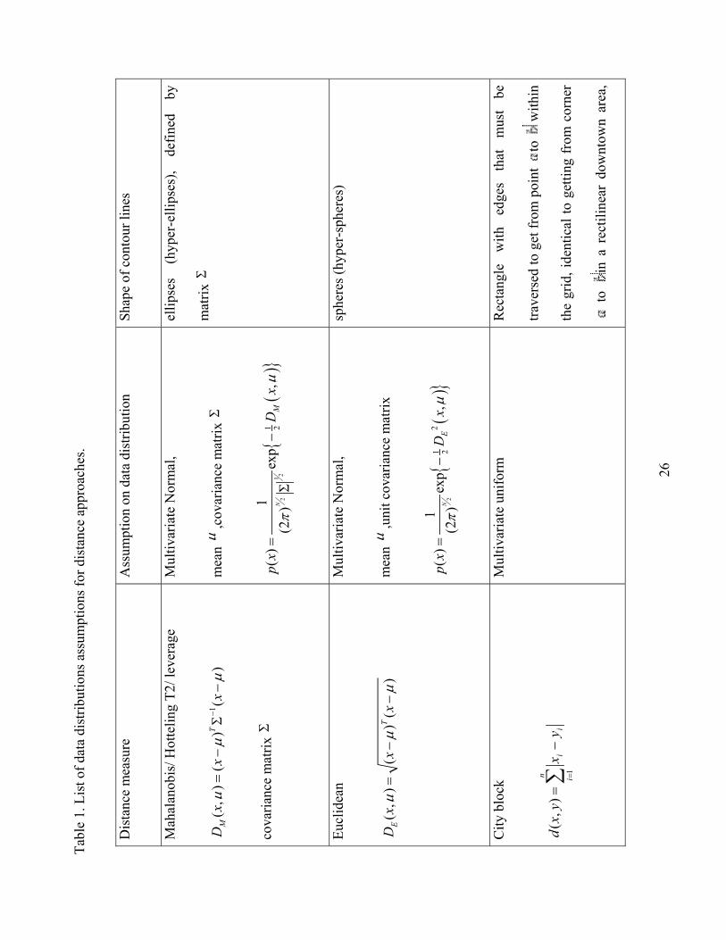
Euclidean and Mahalanobis distance methods identify the interpolation regions assuming that the data is
normally distributed (10,11). City-block distance assumes a triangular distribution. Mahalanobis distance is
unique because it automatically takes into account the correlation between descriptor axes through a
covariance matrix. Other approaches require the additional step of PC rotation to correct for correlated axes.
City block distance is particularly useful for the discrete type of descriptors. The shape of the iso-distance
7

contours, the regions at a constant distance, depends on the particular distance measure used (see Table 1)
and on the particular approach of measuring the distance between a point and a data set.
Hotteling T2/ leverage
Hotelling T2 test and leverage belong to distance methods and their use to assess AD was previously
recommended (12, 13). These measures are proportional to each other and to the Mahalanobis distance.
Hotelling's T2 method is a multivariate Student's-t test and assumes Normal distribution of the data points ().
Leverage approach is also is based on the assumption of a Gaussian data distribution. In regression, the term
leverage values refers to the diagonal elements of the hat matrix H=(X(X'X)-1X'). A given diagonal element
(h(ii)) is represents the distance between X values for the i-th observation and the means of all X values.
These values indicate whether X values could be outliers (14,15). Both Hoteling T2 and leverage are
correcting for collinear descriptors through use of the covariance matrix.
The Hotteling T2 and leverage measure the distance of an observation to the center of X observations. For
Hoteling T2 a tolerance volume is derived. For leverage, most often leverage of 3 is taken as a cut-off value
to accept the points that lay +/- 3 standard deviations from the mean (to cover 99% normally distributed
data).
High leverage values are not always outliers for the model i.e. outside model domain. If high leverage points
fit the model well, (i.e. small residual), they are called “good high leverage points” or good influence points.
Such points will stabilise the model and make it more precise. High leverage points, which do not fit the
8
model (i.e. large residual) are called bad high leverage points or bad influence points. The field of robust
regression provides a number of methods to overcome Hoteling T2 and leverage sensitivity to unusual
observations, but this is out of scope of this paper.
Probability density distribution method
Another method to estimate interpolation region is by probability density. Parametric and nonparametric
methods are the two major approaches. Parametric methods assume that the density function has the shape of
a standard distribution (Gaussian, Poisson, other). Alternatively, a number of nonparametric techniques are
available, which allow the estimation of the probability density solely from data (e.g. kernel density
estimation, mixtures).
Nonparametric probability density estimation is free from any assumptions about data distribution and often
referred as distribution free methods. It is the only approach capable of identifying internal empty regions
within the convex hull. Further, if empty regions are close to the convex hull border nonparametric methods
may generate concave regions to reflect the actual data distribution. In other words, this method captures
actual data distribution. Finally, there is no need to specify a reference point in the data set, rather a
probability value to belong to the set is calculated. Because of these attractive features that other estimation
methods lack we explain probability density estimation in a detail in the Appendix.
Relationships between different interpolation approaches
9
Probability density and all distance based methods yield proportional results if the data are normal
distributed (Table 1) and the distance method uses as a point of reference the distance between a point x and
the data mean. For all other distributions the distance values are neither proportional to p(x) nor they identify
the presence of dense and empty regions. City block distance will vary most from p(x); the degree of the
difference will depend on the specific distribution of the data set. For a comparison, Figure 2 displays AD
regions estimated by Euclidean and Mahalanobis, City block distances and probability distribution based for
the same data set (3, 4).
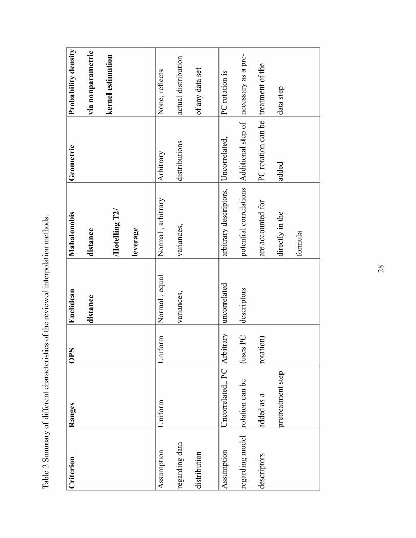
Table 2 summarizes the reviewed methods for assessing interpolation region. In addition, to technical
aspects, we compare software availability for each method. Complexity of approaches varies greatly. This
potentially could turn the user away from the more complex but more flexible ones. We note however,
increasing accessibility to sophisticated numerical methods through software packages so even the most
difficult calculations are becoming possible to apply by nonexperts.
Different results vs. different methods
As we have demonstrated, different interpolation approaches will yield different ADs (Figure 2). This may
leave a reader wondering which method to choose in specific situation. The choice of the particular method
is straightforward: data distribution needs to meet the assumptions of the method.
Although it is straightforward, the requirements for the data distribution in a training set are getting quite
complex. First data has to meet assumptions for a particular model fitting technique. Second, the data has to
10
meet also assumptions of the domain estimation method. As an example, we will use Linear Regression
model as a modelling technique and AD estimation by leverage.
When fitting data to a Linear Regression model with Ordinary Least Squares one first needs to check if: 1)
random error distribution is normal; 2) the mean of the error distribution is zero; 3) The variance of the
random error is equal to a constant for all values of x.; 4) The errors associated with any two different
observations are independent. That is, the error associated with one value of y has no effect on the errors
associated with other values. Assumptions 1 and 2 can be checked with residual analysis. To verify
assumption three requires information about the experimental data measurement error. Different
experimental tests may have different variance and this is a watch out for combining data from different
tests. While assumption 4 is usually satisfied in QSAR research, very few papers check if assumptions 1-3
are satisfied.
Next, a modeller needs to choose a method for the AD estimation that will be suitable to the data
distribution. Let us consider leverage method. The temptation is due to the fact that hat matrix needed to
identify high leverage points (here to be identified as out of the domain) is automatically calculated during
regression model development. However, the method will be suitable only if the data distribution is normal!
Note that in the model development phase developer was checking error distribution not data distribution.
In the past QSAR research verification if a particular training set is adequate for a particular modelling
technique was rare. Rather, tradition and convenience determined the choices. Now with the AD step closely
11
linked to validation we are forced to re-examine existing training sets. It will not come with surprise that
there will be a match between complexity of the training set distribution and complexity of the domain
estimation method. Use of experimental design in a training set would allow modeller to use ranges
approach, lack of representation by any standard distribution may bound the modeller to use a nonparametric
kernel fit.
AD should not be seen as a way to solve deficiencies of existing models. For example, if the existing model
is using collinear descriptors it is the model that needs to be redeveloped so that the descriptors are
orthogonal and not AD correct for this. Running PCA rotation only during AD estimation may result in
difficulties with interpretability of prediction, as the AD would use a reduced number of descriptors. One
possible way forward is to start developing modelling approaches that will allow for simultaneous model
development and AD estimation. Doing it simultaneously will avoid imposing double, often different,
requirements for the data distribution related to model development and next to AD estimation.
Case Study: Various ADs For The Salmonella Mutagenicity Of Aromatic Amines QSAR Model
Debnath et al (3) published mutagenicity model for aromatic and heteroaromatic amines:
log TA98 = 1.08 log P + 1.28EHOMO −0.73ELUMO + 1.46 IL+ 7.20 (1)
where log P – n-octanol/water partition coefficient, HOMO and LUMO – energy on highest occupied and
lowest unoccupied molecular orbitals respectively, IL is an indicator variable and t is 1 for compounds
containing three or more fused rings, and 0 for all other species. N=88, RMSE= 1.059
12

Glende et al (4) studied alkyl-substituted (ortho to the amino function) derivatives not included in original
Debnath database. Most of the new chemicals had descriptors values in the range of original chemicals.
However, with growing steric hindrance of the alkyl groups, the predicted and the experimental values
differed increasingly. Glende’s conclusion was that the QSAR equation is not appropriate to evaluate the
mutagenicity of aromatic amines, substituted with such alkyl groups. Glende’s set was used as a test set
(n=18, RMSE= 2.314).
The AD of the Debnath model was assessed by the following approaches:
1. Ranges in descriptor space and in PC rotated space
2. Euclidean distance in descriptor space and in PC rotated space
3. City-block distance in descriptor space and in PC rotated space
4. Hotelling T2
5. Probability density distribution
We developed different criteria for in and out of the domain appropriate to a given method. For the ranges it
meant that a chemical is out of domain if at least one fragment count and/or correction factors is out of
range or combination of fragments is out of range (this is equivalent to the endpoint value being out of
range). For all distances and Hotelling T2 the cut-off threshold was the largest distance of a training set point
to the center of the training data set (i.e. the distance of the most distant point. For the probabilistic density,
the cut-off threshold was the 95-th and 99-th percentile of probability density of the training set.
13
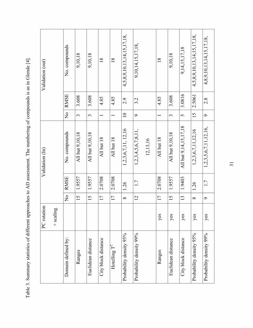
Table 3 summarizes the results of different approaches to define AD by number of chemicals in and out of
the domain, their identification number as well as root mean square error (RMSE).
First, all approaches yield RMSE of out-of-domain validation points higher than RMSE of all validation
points. This means that all approaches are able to identify “out of domain” compounds. However, the RMSE
and number of chemicals out of the domain vary and depend on the method. RMSE from probability density
is the lowest among the methods considered.
As follows, there is a considerable difference in the number of chemicals in the domain between probability
density approach (9 compounds in the domain for 99% cut off) and all others (13-17 in the domain). The
difference reflects the distribution of the data. The analyzed test set lies within the ranges of the training set,
but in empty space (Figure 1). The nonparametric probability density approach is the most suitable method
because data distribution failed normality test. This example is a clear demonstration of the need to check
the distribution of the data first and apply the method that meets the assumptions.
The Figures 3-5 illustrate the correspondence between domain assessment and prediction error for the
evaluated approaches. The upper plots of each group are classic experimental / calculated plots. These plots
show position of the points in and out of domain. In the lower two plots of each group the distance of each
point is plotted against the residual for that compound i.e. prediction error. There is a trend based on
14
average the prediction error in the domain is smaller that out of the domain for all the evaluated methods. In
that sense, the results are similar to findings of Tong et al (6).
DISCUSSION
There are many methods to assess “AD” and confusingly yield different results for the same model. We
examined an approximation of the AD by interpolation of training data set coverage and compared major
multivariate interpolation methods. By focusing on the training set, we did not discuss a particular QSAR
modelling approach. However, we would like to stress out that our discussion is more suited to low
dimension regression and classification models prevalent in modelling safety endpoints (16). The discussion
is less appropriate to partial least squares approach that come with its own set of diagnostic tools such as
distances to the model in x and y space, DMODX and DMODY, respectively (13). Similarly, to partial least
squares approach – DMODY we emphasize the need to include y-space in the AD estimation, particularly in
the interpolation of training set coverage.
The results of AD estimation on the basis of training set coverage reveal a general trend of interpolative
predictive accuracy i.e. concordance between observed and predicted values, was on average greater than
extrapolative predictive accuracy. That however, is only true on average, i.e. there are many individual
compounds with small error outside of the training set coverage, as well as individual compounds with large
error inside the domain.
15

Different interpolation approaches will yield different ADs. The ability of the data distribution should guide
the choice of a particular method. The dimensionality of the model needs to be considered as well. High
dimensionality of the model increases practical numerical complexity especially for geometric and
nonparametric probability density approaches (17).
In addition, there is a need to reconcile the methods used for model development (fit) and methods used to
estimate the AD. Separate treatment of these two steps often poses different requirements for the data
distribution in the training set making it a very demanding to meet all the assumptions. Joint fit and
estimation of AD by probability density methods is a promising approach (Aldenberg – personal
communication). This area requires more attention and further work.
By identification of the data set coverage, we make only a partial step towards defining the AD of a model.
There is always a possibility that the model is missing a descriptor needed to correctly predict a queried
chemical’s activity and despite the chemical being in the domain, the chemical’s activity will be predicted
with error. There is also always another possibility that the model extrapolates correctly outside the domain.
Therefore, in order to describe the domain more robustly, the full training set comprising both structures and
descriptor set is required. The full training set allows assessing its chemical space coverage. What we have
not discussed in this paper is the need for a global structural similarity test to ensure that the structural
features in a new test compound are covered in the original training set of chemicals, (a quantitative measure
of uniqueness relative to the training set) (D. Stanton – personal communication). The global similarity test
16

should be sufficiently robust to cover general chemistry. These two conditions: 1) being in the training set
coverage and 2) structural similarity are complementary and need not be carried out in any particular order.
However, we recommend use of different methodologies to examine training set in different ways and
maximize the chances to find a potential difference.
The discussed methodologies will help to provide us with warnings to confirm whether a chemical is inside
or outside the domain. However, they are not final measures for acceptance or rejection of a prediction. In
other words, however robust the methods become they will never enable the end user to make an ultimate
decision about a chemical. The reason for this is because we only possess the knowledge of the training size
and we do not possess the knowledge of when the model breaks down.
Acknowledgment
Funding for Nina Nikolova-Jeliazkowa was provided by Procter & Gamble as postdoctoral fellowship. All
authors acknowledge ECVAM for partial funding of this work under contract CCR.496575-Z. We thank Dr.
A. Benigni for drawing our attention to the chosen case study.
Appendix
Probability density estimation
Density estimation is an area of extensive research. Due to computational challenges most methods focus on
low dimensional (1-, 2-, 3- ) densities, unless additional assumptions are made (17). Recently developed
17
Algorithm for Multivariate Kernel Density Estimation (18,19, 20) achieves several orders of magnitude
speed improvement by using computational geometry to organize the data. This method estimates directly
true multivariate density and is very accurate. Appendix illustrates the need to be very transparent about data
processing during density estimation as different results can be obtained.
The kernel density estimation method.
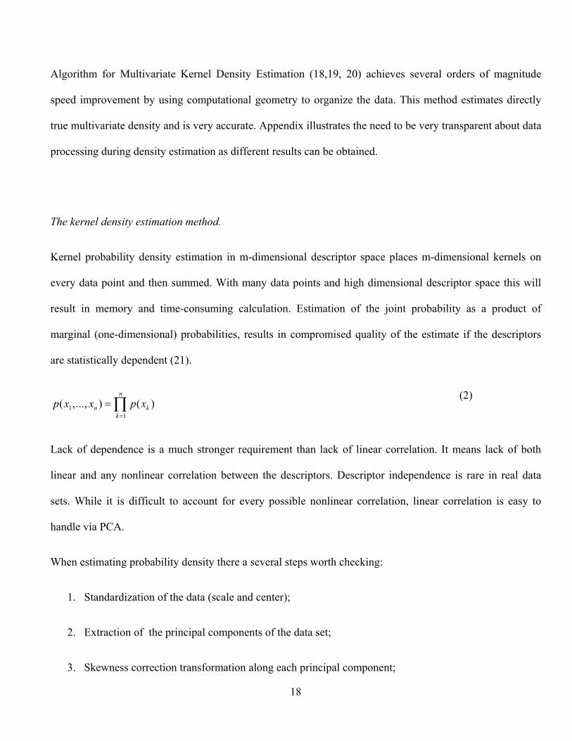
Kernel probability density estimation in m-dimensional descriptor space places m-dimensional kernels on
every data point and then summed. With many data points and high dimensional descriptor space this will
result in memory and time-consuming calculation. Estimation of the joint probability as a product of
marginal (one-dimensional) probabilities, results in compromised quality of the estimate if the descriptors
are statistically dependent (21).
11
( ,..., ) ( )n
n kk
p x x p x=
=∏
(2)
Lack of dependence is a much stronger requirement than lack of linear correlation. It means lack of both
linear and any nonlinear correlation between the descriptors. Descriptor independence is rare in real data
sets. While it is difficult to account for every possible nonlinear correlation, linear correlation is easy to
handle via PCA.
When estimating probability density there a several steps worth checking:
1. Standardization of the data (scale and center);
2. Extraction of the principal components of the data set;
3. Skewness correction transformation along each principal component;
18
4. Estimation the one-dimensional density on each transformed principal component;
Figure 6 illustrates three projections of probability density with growing degree of accuracy. The density,
obtained as the product of 1D densities in the original descriptor space is shown on 6 a., The estimated
density does not reflect the actual data density because the parameters are dependent. Figure 6b displays the
density obtained as sum of Gaussian kernels in PC space. Figure 6 c shows improved quality of the
estimated density by employing data set transformations like data standardization and skewness correction.
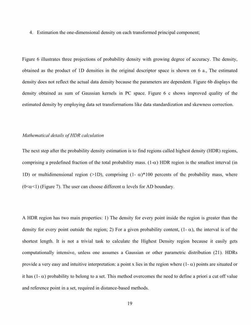
Mathematical details of HDR calculation
The next step after the probability density estimation is to find regions called highest density (HDR) regions,
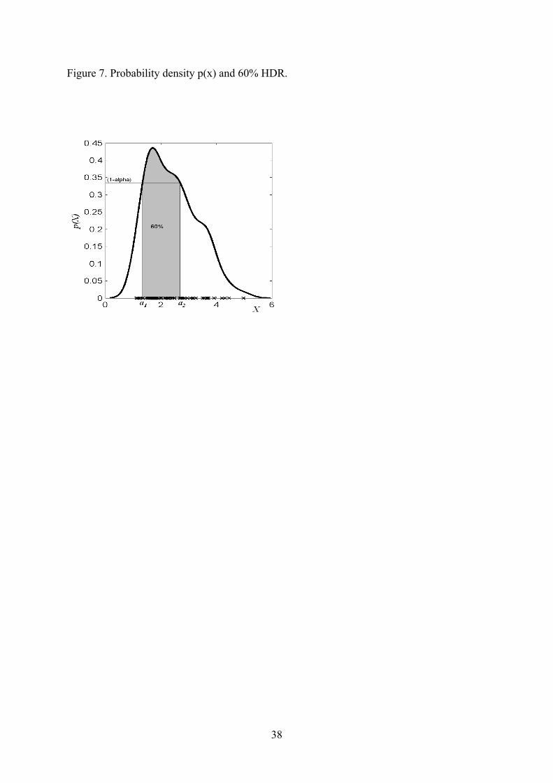
comprising a predefined fraction of the total probability mass. (1-α) HDR region is the smallest interval (in
1D) or multidimensional region (>1D), comprising (1- α)*100 percents of the probability mass, where
(0<α<1) (Figure 7). The user can choose different α levels for AD boundary.
A HDR region has two main properties: 1) The density for every point inside the region is greater than the
density for every point outside the region; 2) For a given probability content, (1- α), the interval is of the
shortest length. It is not a trivial task to calculate the Highest Density region because it easily gets
computationally intensive, unless one assumes a Gaussian or other parametric distribution (21). HDRs
provide a very easy and intuitive interpretation: a point x lies in the region where (1- α) points are situated or
it has (1- α) probability to belong to a set. This method overcomes the need to define a priori a cut off value
and reference point in a set, required in distance-based methods.
19
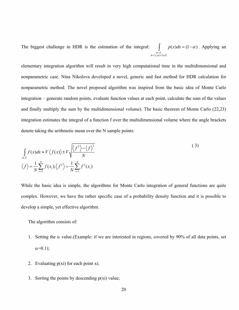
The biggest challenge in HDR is the estimation of the integral:,
{ : ( ) }
( ) (1 )x A
A x p x d
p x dx α∈
= ≤
= −∫ . Applying an
elementary integration algorithm will result in very high computational time in the multidimensional and
nonparametric case. Nina Nikolova developed a novel, generic and fast method for HDR calculation for
nonparametric method. The novel proposed algorithm was inspired from the basic idea of Monte Carlo
integration – generate random points, evaluate function values at each point, calculate the sum of the values
and finally multiply the sum by the multidimensional volume). The basic theorem of Monte Carlo (22,23)
integration estimates the integral of a function f over the multidimensional volume where the angle brackets
denote taking the arithmetic mean over the N sample points:
22
2 2
1 1
( ) ( )
1 1( ); ( )
x SN N
i ii i
f ff x dx V f x V
N
f f x f f xN N
∈
= =
−≈ ±
= =
∫
∑ ∑
( 3)
While the basic idea is simple, the algorithms for Monte Carlo integration of general functions are quite
complex. However, we have the rather specific case of a probability density function and it is possible to
develop a simple, yet effective algorithm.
The algorithm consists of:
1. Setting the α value.(Example: if we are interested in regions, covered by 90% of all data points, set
α=0.1);
2. Evaluating p(xi) for each point xi;
3. Sorting the points by descending p(xi) value;
20

4. Counting the first M points belonging to the (1-α) fraction of all the points;
The smallest p(xi) of this (1-α) set is the threshold value d= D(1-α). For a query point y, calculate p(y) is
calculated. If p(y) ≥ D (1- α) then the point is within the dense region comprising (1- α) of all the data points
probability mass.
The density value d= D(1-α) is sufficient to assess whether a query point y will fall within (1-α) Highest
Density Region. That is, we are able to assess whether a new compound is inside or outside the descriptor
space covered by a given data set. The thresholds D(1-α) for different α can be stored and used for further
evaluation of query points. The knowledge of the density value is also sufficient for HDR visualization (24).
Structures of the Glende et al. 2001 test set.
Structure R No Compound Abbreviation
NH2
H
Et
1
2
2-Aminonaphtalene
1-Ethyl 2-aminonaphtalene
2-AN
1-Et-2AN
21

iPr
nBu
tBu
3
4
5
1-iPropyl 2-aminonaphtalene
1-nButyl 2-aminonaphtalene
1-tBu 2-aminonaphtalene
1-iPr-2AN
1-nBu-2AN
1-tBu-2AN
RNH2
H
Et
iPr
nBu
tBu
6
7
8
9
10
2-Aminofluorene
1-Ethyl 2- aminofluorene
1-iPropyl 2- aminofluorene
1-nButyl 2- aminofluorene
1-tBu 2- aminofluorene
2-AF
1-Et-2 AF
1-iPr-2 AF
1-nBu-2 AF
1-tBu-2 AF
R
NH2
H
Et
iPr
nBu
tBu
11
12
13
14
15
4-Aminobiphenyl
3-Ethyl-4-aminobiphenyl
3-iPropyl-4-aminobiphenyl
1-nButyl 2- aminobiphenyl
1-tBu 2- aminobiphenyl
4-ABP
3-Et-4 ABP
3-iPr-4 ABP
3-nBu-4 ABP
3-tBu-4 ABP
R
NH2
R
Me
Et
iPr
16
17
18
3,5-Dimethyl-4-aminobiphenyl
3,5-Diethyl-4-aminobiphenyl
3,5-DiiPropyl-4-aminobiphenyl
3.5-diMe-4ABP
3.5-diEt-4-ABP
3.5-diiPr-4-ABP
22

References
1. Cefic (2002). (Q)SARs for Human Health and the Environment. In Workshop Report on Regulatory
acceptance of (Q)SARs Setubal, Portugal, March 4-6, 2002
2. Nikolova, N. & Jaworska, J. (2002). Review of chemical similarity measures, QSAR &
Combinatorial Science, 22, 1006-1026.
3. Debnath, A.K., Debnath, G., Shusterman, A.J. & Hansch, C. (1992). A QSAR investigation of the
role of hydrophobicity in regulating mutagenicity in the Ames test: 1. Mutagenicity of aromatic and
heteroaromatic amines in Salmonella typhimurium TA98 and TA100. Environmental Molecular
Mutagenesis. 19, 37-52.
4. Glende, C, Schmitt, H., Erdinger, L., Engelhardt, G. & Boche G. (2001). Transformation of
mutagenic aromatic amines into non-mutagenic species by alkyl substituents. Part I. Alkylation ortho
to the amino function. Mutation Research, 498, 19-37.
5. TOPKAT OPS (2000) , US patent no. 6 036 349 issued March 14, 2000
6. Tong W., Qian X., Huixiao H., Leming S., Hong F., Perkins R. (2004) Assessment of Prediction
Confidence and Domain Extrapolation of Two Structure–Activity Relationship Models for Predicting
Estrogen Receptor Binding Activity, Environmental Health Perspectives, 112(12), 1249-1254
7. Tunkel (2004) Practical Considerations on the Use of Predictive Models for Regulatory Purposes,
Presentation at QSAR 2004, Liverpool, UK
8. Nikolova, N. & Jaworska, J. (2005), An approach to determine AD for QSAR group contribution
models: an analysis of SRC KOWWIN, Alternatives to Laboratory Animals (this issue)
23
9. Preparata F.P. & Shamos M.I., (1991). Computational Geometry: An Introduction, pp398, Chapter 3
Convex Hulls: Basic Algorithms, p.95-148, New-York : Springer-Verlag
10. Fukunaga, K. (1990). Introduction to Statistical Pattern Recognition, 2nd ed. pp. 592, Computer
Science and Scientific Computing Series, New York, Academic Press.
11. Seber, G.A.F. (1984). Multivariate Observations, pp712, New York, NY, USA, John Wiley & Sons.
12. Tropsha A., Gramatica P. & Gombar V. (2003). The Importance of Being Earnest: validation is the
Absolute Essential for Successful Application and interpretation of QSPR Models. QSAR &
Combinatorial Sciences, 22, 69-77.
13. Eriksson, L., Jaworska, J., Worth, A., Cronin, M.T.D., McDowell, R.M. & Gramatica, P., (2003)
Methods for Reliability and Uncertainty Assessment and for Applicability Evaluations of
Classification- and Regression- Based QSARs. Environmental Health Perspectives, 111, No. 10,
1351–1375.
14. Neter, J., Kutner, M. H., Wasserman, W., Nachtsheim C., (1996), Applied Linear Statistical Models,
pp1408, McGraw-Hill, Irwin.
15. Myers, R.H. (2000). Classical and Modern Regression with Applications, 2nd ed., pp. 488, Duxbury
Press, UK
16. ECETOC (2003). Evaluation of commercially available software for human health, environmental
and physico-chemical endpoints. ECETOC QSAR TF report nr 89 (chair J. Jaworska), 164 pp.,
Brussels, Belgium
17. Silverman, B.W. (1986). Density Estimation for Statistics and Data Analysis, pp 176 Chapman &
Hall/CRC, London, UK
24

18. Gray, A., Moore, A. (2003a). Nonparametric Density Estimation: Toward Computational
Tractability, Proc. SIAM International Conference on Data Mining, San Francisco, USA,
19. Gray, A., Moore, A. (2003b). Very Fast Multivariate Kernel Density Estimation via Computational
Geometry, in Proceedings Joint Statistical Meeting, Aug 3-7,2003 , San Francisco, USA
20. Ihler A. (2004). MATLAB KDE class, Website http://ssg.mit.edu/~ihler/code/kde.shtml (Accessed 27
Jan 2005).
21. Friedman, J.H. (1987). Exploratory projection pursuit. Journal of the American Statistic Association
82, 249-266.
22. Chen, M.-H. & Shao, Q-M. (1999). Monte Carlo Estimation of Bayesian Credible and HPD
Intervals. Journal of Computational and Graphical Statistics, 8, No.1, 69-92
23. Weinzierl, S. (2000), "Introduction to Monte Carlo Methods.", Website http://arxiv.org/abs/hep-
ph/0006269 (Accessed 27 Jan 2005)
24. Press, W., Teukolsky, S., Vetterling, W., Flannery, B. (1992). Numerical Recipes in C: The Art of
Scientific Computing, 2nd ed, pp1020, Cambridge University Press, UK
25
Tabl
e 1.
Lis
t of d
ata
dist
ribut
ions
ass
umpt
ions
for d
ista
nce
appr
oach
es.
Dis
tanc
e m
easu
re
Ass
umpt
ion
on d
ata
dist
ribut
ion
Shap
e of
con
tour
line
s
Mah
alan
obis
/ Hot
telin
g T2
/ lev
erag
e
1(
,)
()
()
TM
Dx
xx
µµ
µ−
=−
Σ−
cova
rianc
e m
atrix
Σ
Mul
tivar
iate
Nor
mal
,
mea
n µ
,cov
aria
nce
mat
rix Σ
()
{}
1 22
1 21
()
exp
,(2
)NM
px
Dxµ
π=
−Σ
ellip
ses
(hyp
er-e
llips
es),
defin
ed
by
mat
rix Σ
Eucl
idea
n
(,
)(
)(
)T
ED
xx
xµ
µµ
=−
−
Mul
tivar
iate
Nor
mal
,
mea
n µ
,uni
t cov
aria
nce
mat
rix
()
{}
2
21 2
1(
)ex
p,
(2)N
Ep
xD
xµ
π=
−
sphe
res (
hype
r-sp
here
s)
City
blo
ck ∑ =
−=
n ii
iy
xy
xd
1)
,(
Mul
tivar
iate
uni
form
R
ecta
ngle
w
ith
edge
s th
at
mus
t be
trave
rsed
to g
et fr
om p
oint
to
w
ithin
the
grid
, ide
ntic
al to
get
ting
from
cor
ner
to
in a
rec
tilin
ear
dow
ntow
n ar
ea,
26

henc
e th
e na
me
“city
-blo
ck m
etric
.”
27
Tabl
e 2
Sum
mar
y of
diff
eren
t cha
ract
eris
tics o
f the
revi
ewed
inte
rpol
atio
n m
etho
ds.
Cri
teri
on
Ran
ges
OPS
E
uclid
ean
dist
ance
Mah
alon
obis
dist
ance
/Hot
ellin
g T
2/
leve
rage
Geo
met
ric
Pr
obab
ilit y
den
sity
via
nonp
aram
etri
c
kern
el e
stim
atio
n
Ass
umpt
ion
rega
rdin
g da
ta
dist
ribut
ion
Uni
form
U
nifo
rm
Nor
mal
, eq
ual
varia
nces
,
Nor
mal
, ar
bitra
ry
varia
nces
,
Arb
itrar
y
dist
ribut
ions
Non
e, re
flect
s
actu
al d
istri
butio
n
of a
ny d
ata
set
Ass
umpt
ion
rega
rdin
g m
odel
desc
ripto
rs
Unc
orre
late
d,, P
C
rota
tion
can
be
adde
d as
a
pret
reat
men
t ste
p
Arb
itrar
y
(use
s PC
rota
tion)
unco
rrel
ated
desc
ripto
rs
arbi
trary
des
crip
tors
,
pote
ntia
l cor
rela
tions
are
acco
unte
d fo
r
dire
ctly
in th
e
form
ula
Unc
orre
late
d,
Add
ition
al st
ep o
f
PC ro
tatio
n ca
n be
adde
d
PC ro
tatio
n is
nece
ssar
y as
a p
re-
treat
men
t of t
he
data
step
28

abili
ty to
disc
over
inte
rnal
dens
e an
d sp
arse
regi
ons o
f the
inte
rpol
ated
spac
e
no
no
nono
noye
s
Abi
lity
to
quan
tify
dist
ance
from
the
cent
er o
f
the
set
no
ye
sye
sye
sno
Yes
easi
ness
of
appl
icat
ion
of th
e
met
hod
in m
any
dim
ensi
ons
easy
ea
sy
easy
Ea
sy, i
nvol
ves
inve
rsio
n of
the
cova
rianc
e m
atrix
(cou
ld b
e sl
ow fo
r
man
y di
men
sion
s)
diff
icul
t abo
ve 3
D
Use
d to
be
diff
icul
t
abov
e 3d
;
A re
cent
ver
y fa
st
met
hod
in M
atla
b
wor
ks in
man
y
dim
ensi
ons
29

Ava
ilabi
lity
of
tool
s i.e
. sof
twar
e
usin
g th
e m
etho
d. St
atis
tical
softw
are
for
gene
ral u
se
TOPK
AT
S
tatis
tical
softw
are
for
gene
ral u
se
Sta
tistic
al so
ftwar
e
for g
ener
al u
se, m
ay
requ
ire so
me
prog
ram
min
g
Com
puta
tiona
l
geom
etry
pack
ages
; mos
t
mat
hem
atic
al
pack
ages
Mat
lab,
Mat
hem
atic
a
HD
R c
alcu
latio
n
requ
ires
prog
ram
min
g
30
Tabl
e 3.
Sum
mar
y st
atis
tics o
f diff
eren
t app
roac
hes t
o A
D a
sses
smen
t. Th
e nu
mbe
ring
of c
ompo
unds
is a
s in
Gle
nde
[4].
PC ro
tatio
n
+ sc
alin
g
Val
idat
ion
(In)
V
alid
atio
n (o
ut)
Dom
ain
defin
ed b
y:
N
oR
MSE
N
o. c
ompo
unds
N
oR
MSE
No.
com
poun
ds
Ran
ges
15
1.
9557
A
ll bu
t 9,1
0,18
3
3.60
8 9,
10,1
8
Eucl
idea
n di
stan
ce
15
1.
9557
A
ll bu
t 9,1
0,18
3
3.60
8 9,
10,1
8
City
blo
ck d
ista
nce
17
2.
0708
A
ll bu
t 18
1 4.
85
18
Hot
ellin
g T2
17
2.
0708
A
ll bu
t 18
1 4.
85
18
Prob
abili
ty d
ensi
ty 9
5%
8
1.26
1,
2,3,
6,7,
11, 1
2,16
10
2.
9 4,
5,8,
9,10
,13,
14,1
5,17
,18,
Prob
abili
ty d
ensi
ty 9
9%
12
1.
7 1,
2,3,
4,5,
6,7,
8,11
,
12,1
3,16
9
3.
29,
10,1
4,15
,17,
18,
Ran
ges
yes
17
2.07
08
All
but 1
8 1
4.85
18
Eucl
idea
n di
stan
ce
yes
15
1.95
57
All
but 9
,10,
18
3 3.
608
9,10
,18
City
blo
ck d
ista
nce
yes
13
1.94
03
All
but 9
,14,
15,1
7,18
5
3.08
169,
14,1
5,17
,18
Prob
abili
ty d
ensi
ty 9
5%
yes
8 1.
26
1,2,
3,6,
7,11
,12,
16
15
2.50
614,
5,8,
9,10
,13,
14,1
5,17
,18,
Prob
abili
ty d
ensi
ty 9
9%
yes
9 1.
7 1,
2,3,
5,6,
7,11
,12,
16,
9 2.
8 4,
8,9,
10,1
3,14
,15,
17,1
8,
31

Figure 1. A eLUMO- Log P 2D projection of a training data set chemicals (3) - and test set
chemicals from (4) - .
.
32
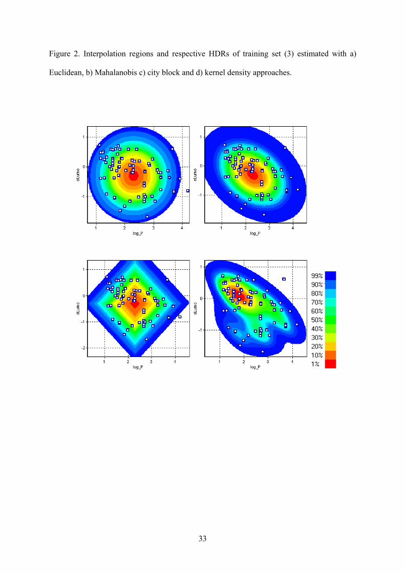
Figure 2. Interpolation regions and respective HDRs of training set (3) estimated with a)
Euclidean, b) Mahalanobis c) city block and d) kernel density approaches.
33
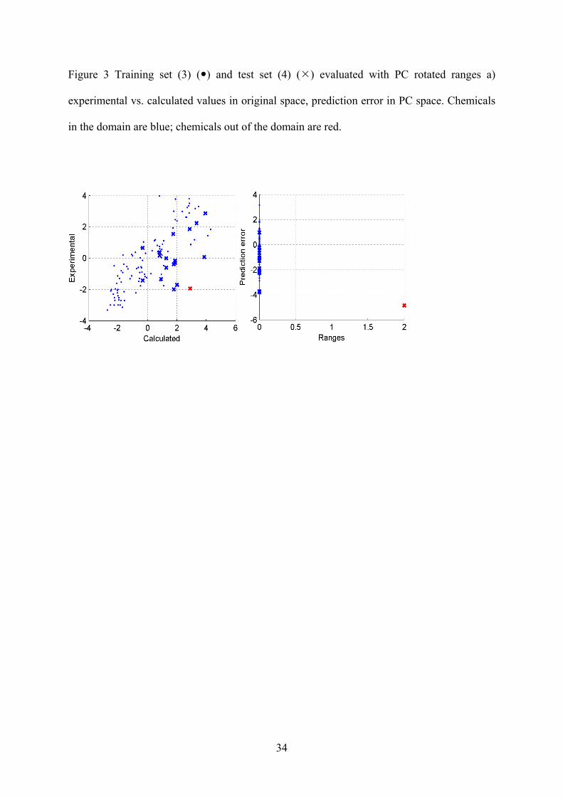
Figure 3 Training set (3) ( ) and test set (4) ( ) evaluated with PC rotated ranges a)
experimental vs. calculated values in original space, prediction error in PC space. Chemicals
in the domain are blue; chemicals out of the domain are red.
34
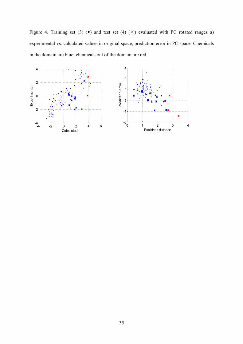
Figure 4. Training set (3) ( ) and test set (4) ( ) evaluated with PC rotated ranges a)
experimental vs. calculated values in original space, prediction error in PC space. Chemicals
in the domain are blue; chemicals out of the domain are red.
35
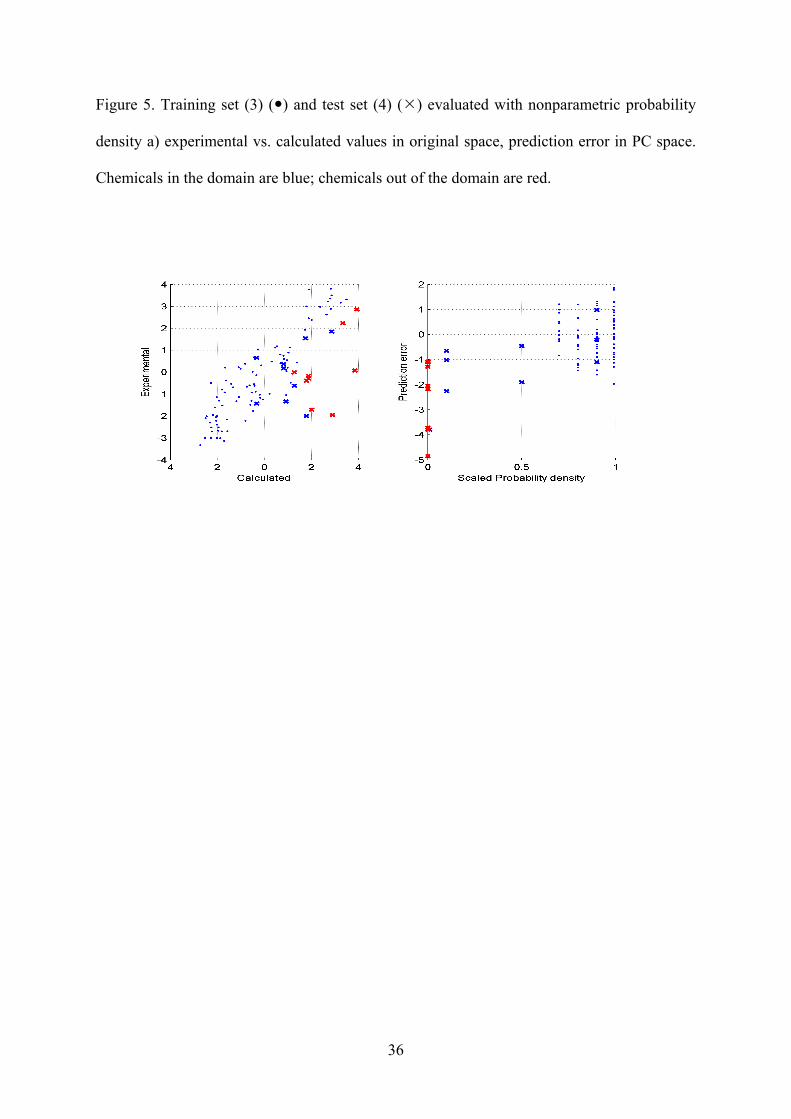
Figure 5. Training set (3) ( ) and test set (4) ( ) evaluated with nonparametric probability
density a) experimental vs. calculated values in original space, prediction error in PC space.
Chemicals in the domain are blue; chemicals out of the domain are red.
36
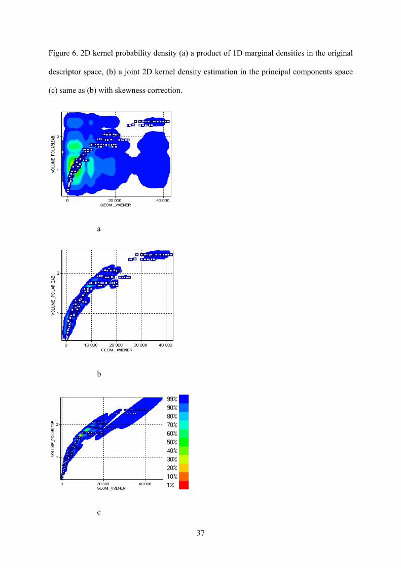
Figure 6. 2D kernel probability density (a) a product of 1D marginal densities in the original
descriptor space, (b) a joint 2D kernel density estimation in the principal components space
(c) same as (b) with skewness correction.
a
b
c
37
38
Figure 7. Probability density p(x) and 60% HDR.