Review - Jean-Luc Starckjstarck.free.fr/pasp02.pdf · 1052 STARCK, PANTIN, & MURTAGH 2002 PASP, 114:1051–1069 Fig. 1.—Active galactic nucleus of NGC 1068 observed at 20 mm. Left:

1051

Publications of the Astronomical Society of the Pacific, 114:1051–1069, 2002 October� 2002. The Astronomical Society of the Pacific. All rights reserved. Printed in U.S.A.

Review

Deconvolution in Astronomy: A Review

J. L. Starck and E. Pantin

Service d’Astrophysique, SAP/SEDI, CEA-Saclay, F-91191 Gif-sur-Yvette Cedex, France; [email protected], [email protected]

andF. Murtagh

School of Computer Science, Queen’s University Belfast, Belfast BT7 1NN, Northern Ireland; and Observatoire de Strasbourg,UniversiteLouis Pasteur, F-67000 Strasbourg, France; [email protected]

Received 2002 March 21; accepted 2002 June 28

ABSTRACT. This article reviews different deconvolution methods. The all-pervasive presence of noise is whatmakes deconvolution particularly difficult. The diversity of resulting algorithms reflects different ways ofestimating the true signal under various idealizations of its properties. Different ways of approaching signalrecovery are based on different instrumental noise models, whether the astronomical objects are pointlike orextended, and indeed on the computational resources available to the analyst. We present a number of recentresults in this survey of signal restoration, including in the areas of superresolution and dithering. In particular,we show that most recent published work has consisted of incorporating some form of multiresolution in thedeconvolution process.

1. INTRODUCTION

Deconvolution is a key area in signal and image processing.It is used for objectives in signal and image processing thatinclude the following:

1. deblurring,2. removal of atmospheric seeing degradation,3. correction of mirror spherical aberration,4. image sharpening,5. mapping detector response characteristics to those of

another,6. image or signal zooming, and7. optimizing display.

In this article, we focus on one particular but central interfacebetween model and observational data. In observationalastronomy, modeling embraces instrument models and also in-formation registration and correlation between different datamodalities, including image and catalog. The measure of ob-serving performance that is of greatest interest to us in thiscontext is the instrument degradation function, or point-spreadfunction. How the point-spread function is used to improveimage or signal quality lies in deconvolution. We will reviewa range of important recent results in deconvolution. A centraltheme for us is how nearly all deconvolution methods, arisingfrom different instrument noise models or from priority givento point-source or extended objects, now incorporate resolutionscale into their algorithms. Some other results are very excitingtoo. A recent result of importance is the potential for super-resolution, characterized by a precise algorithmic definition of

the “near-black object.” A further result of note is dithering asa form of stochastic resonance and not just as a purely ad hocapproach to getting a better signal.

Deconvolution of astronomical images has proven in somecases to be crucial for extracting scientific content. For instance,IRAS images can be efficiently reconstructed thanks to a newpyramidal maximum entropy algorithm (Bontekoe, Koper, &Kester 1994). Io volcanism can be studied with a lower res-olution of 0�.15, or 570 km on Io (Marchis, Prange´, & Christou2000). Deconvolved mid-infrared images at 20mm revealedthe inner structure of the active galactic nucleus in NGC 1068,hidden at lower wavelength because of the high extinction(Alloin et al. 2000; see Fig. 1). Research on gravitational lensesis easier and more efficient when applying deconvolution meth-ods (Courbin, Lidman, & Magain 1998). A final example isthe high resolution (after deconvolution) of mid-infraredimages revealing the intimate structure of young stellar objects(Zavagno, Lagage, & Cabrit 1999). Deconvolution will be evenmore crucial in the future in order to fully take advantage ofincreasing numbers of high-quality ground-based telescopes,for which images are strongly limited in resolution by theseeing.

The Hubble Space Telescope (HST ) provided a leading ex-ample of the need for deconvolution in the period before thedetector system was refurbished. Two proceedings (White &Allen 1990; Hanisch & White 1994) provide useful overviewsof this work, and a later reference is Adorf, Hook, & Lucy(1995). While an atmospheric seeing point-spread function(PSF) may be relatively tightly distributed around the mode,

1052 STARCK, PANTIN, & MURTAGH

2002 PASP,114:1051–1069

Fig. 1.—Active galactic nucleus of NGC 1068 observed at 20mm. Left: Raw image is highly blurred by telescope diffraction.Right: Restored image using themultiscale entropy method reveals the inner structure in the vicinity of the nucleus.

this was not the case for the spherically aberratedHST PSF.Whenever the PSF “wings” are extended and irregular, decon-volution offers a straightforward way to mitigate the effects ofthis and to upgrade the core region of a point source. One usageof deconvolution of continuing importance is in informationfusion from different detectors. For example, Faure et al. (2002)deconvolveHST images when correlating with ground-basedobservations. In Radomski et al. (2002), Keck data are decon-volved for study withHST data. VLT data are deconvolved inBurud et al. (2002), with other ESO andHST data used aswell. In planetary work, Coustenis et al. (2001) discuss CFHTdata as well asHST and other observations.

What emerges very clearly from this small sample—whichis in no way atypical—is that a major use of deconvolution isto help in cross-correlating image and signal information.

An observed signal is never in pristine condition, andimproving it involves inverting the spoiling conditions, i.e.,finding a solution to an inverse equation. Constraints relatedto the type of signal we are dealing with play an importantrole in the development of effective and efficient algorithms.The use of constraints to provide for a stable and unique so-lution is termed regularization. Examples of commonly usedconstraints include a result image or signal that is nonnegativeeverywhere, an excellent match to source profiles, necessarystatistical properties (Gaussian distribution, no correlation, etc.)for residuals, and absence of specific artifacts (ringing aroundsources, blockiness, etc.).

Our review opens in § 2 with a formalization of the problem.In § 3, we consider the issue of regularization. In § 4, theCLEAN method, which is central to radio astronomy, is de-scribed. Bayesian modeling and inference in deconvolution isreviewed in § 5. In § 6, we introduce wavelet-based methodsas used in deconvolution. These methods are based on multipleresolution or scale. In §§ 7 and 8, important issues related toresolution of the output result image are discussed. Section 7

is based on the fact that it is normally not worthwhile to targetan output result with better resolution than some limit, forinstance, a pixel size. In § 8, we investigate when, where, andhow missing information can be inferred to providesuperresolution.

2. THE DECONVOLUTION PROBLEM

Noise is the bane of the image analyst’s life. Without it wecould so much more easily rectify data, compress them, andinterpret them. Unfortunately, however, deconvolution becomesa difficult problem due to the presence of noise in high-qualityor deep imaging.

Consider an image characterized by its intensity distribution(the “data”) I, corresponding to the observation of a “realimage” O through an optical system. If the imaging system islinear and shift-invariant, the relation between the data and theimage in the same coordinate frame is a convolution:

��

I(x, y) p P(x � x , y � y )O(x , y )dx dy� � 1 1 1 1 1 1x p�� y p��1 1

� N(x, y)

p (P ∗ O)(x, y) � N(x, y), (1)

whereP is the PSF of the imaging system andN is additivenoise.

In Fourier space, we have

ˆˆ ˆ Î(u, v) p O(u, v)P(u, v) � N(u, v). (2)

We want to determine knowingI andP. This inverseO(x, y)problem has led to a large amount of work, the main difficultiesbeing the existence of (1) a cutoff frequency of the PSF and(2) the additive noise (see, for example, Cornwell 1989;

DECONVOLUTION IN ASTRONOMY 1053

2002 PASP,114:1051–1069

Katsaggelos 1993; Bertero & Boccacci 1998; Molina et al.2001).

A solution can be obtained by computing the Fourier trans-form of the deconvolved object by a simple division betweenOthe image and the PSF :ˆ Î P

ˆ Î(u, v) N(u, v)ˆ Ô(u, v) p p O(u, v) � . (3)ˆ ˆP(u, v) P(u, v)

This method, sometimes called theFourier-quotient method,is very fast. We need to do only a Fourier transform and aninverse Fourier transform. For frequencies close to the fre-quency cutoff, the noise term becomes important, and the noiseis amplified. Therefore, in the presence of noise, this methodcannot be used.

Equation (1) is usually in practice an ill-posed problem. Thismeans that there is no unique and stable solution.

The diversity of algorithms to be looked at in the followingsections reflects different ways of recovering a “best” estimateof the source. If one has good prior knowledge, then simplemodeling of PSF-convolved sources with a set of variableparameters is often used. In fact, this is often a favored ap-proach, in order to avoid deconvolution, even though its usersare unaware of the consequences of its spatially correlatedresiduals. Lacking specific source information, one then relieson general properties, which have been referred to in § 1. Thealgorithms described in our review approach these issues indifferent ways.

With linear regularized methods (§ 3) we use a smoothing/sharpening trade-off. CLEAN assumes our objects are pointsources. We discuss the powerful Bayesian methodology interms of different noise models that can be applicable. Maxi-mum entropy makes a very specific assumption about sourcestructure, but in at least its traditional formulations it was poorat addressing the expected properties of the residuals producedwhen the estimated source was compared to the observations.Some further work is reviewed that models planetary imagesor extended objects. So far, all of these methods work, usuallyiteratively, on the given data.

The story of § 6 is an answer to the question: Where andhow do we introduce resolution scale into the methods wereview in § 3, 4, and 5, and what are the benefits of doingthis?

Some varied directions that deconvolution can take are asfollows:

1. Superresolution: object spatial frequency information out-side the spatial bandwidth of the image formation system isrecovered.

2. Blind deconvolution: the PSFP is unknown.3. Myopic deconvolution: the PSFP is partially known.4. Image reconstruction: an image is formed from a series

of projections (computed tomography, positron emissiontomography [PET], and so on).

We will discuss only the deconvolution and superresolutionproblems in this paper.

In the deconvolution problem, the PSF is assumed to beknown. In practice, we have to construct a PSF from the dataor from an optical model of the imaging telescope. In astron-omy, the data may contain stars, or one can point toward areference star in order to reconstruct a PSF. The drawback isthe “degradation” of this PSF because of unavoidable noise orspurious instrument signatures in the data. So, when recon-structing a PSF from experimental data, one has to reduce verycarefully the images used (background removal, for instance)or otherwise any spurious feature in the PSF would be repeatedaround each object in the deconvolved image. Another problemarises when the PSF is highly variable with time, as is the casefor adaptive optics images. This usually means that the PSFestimated when observing a reference star, after or before theobservation of the scientific target, hassmall differences froma perfect PSF. In this particular case, one has to turn towardmyopic deconvolution methods (Christou et al. 1999) inwhich the PSF is also estimated in the iterative algorithmusing a first guess deduced from observations of referencestars.

Another approach consists of constructing a synthetic PSF.Several studies (Buonanno et al. 1983; Moffat 1969; Djorgov-ski 1983; Molina et al. 1992) have suggested a radially sym-metric approximation to the PSF:

�b2r

P(r) ∝ 1 � . (4)2( )R

The parametersb andR are obtained by fitting the model withstars contained in the data.

3. LINEAR REGULARIZED METHODS

It is easy to verify that the minimization ofk I(x, y) �, where the asterisk means convolution,2P(x, y) ∗ O(x, y)k

leads to the least-squares solution:

∗ˆ ˆP (u, v)I(u, v)Ô(u, v) p , (5)2ˆd P(u, v)F

which is defined only if (the Fourier transform of theP(u, v)PSF) is different from zero. A tilde indicates an estimate. Theproblem is generally ill-posed and we need to introducereg-ularization in order to find a unique and stable solution.

Tikhonov regularization (Tikhonov et al. 1987) consists ofminimizing the term

J (O) pk I(x, y) � (P ∗ O)(x, y) k �l k H ∗ O k , (6)T

whereH corresponds to a high-pass filter. This criterion con-tains two terms. The first, ,2kI(x, y) � P(x, y) ∗ O(x, y)kexpresses fidelity to the data , and the second,I(x, y)


2002 PASP,114:1051–1069

, expresses smoothness of the restored image;l is2l k H ∗ Okthe regularization parameter and represents the trade-off be-tween fidelity to the data and the smoothness of the restoredimage. The solution is obtained directly in Fourier space:

∗ˆ ˆP (u, v)I(u, v)Ô(u, v) p . (7)2 2ˆ ˆd P(u, v)F � l d H(u, v)F

Finding the optimal valuel necessitates use of numericaltechniques such as cross-validation (Golub, Heath, & Wahba1979; Galatsanos & Katsaggelos 1992). This method workswell, but computationally it is relatively lengthy and producessmoothed images. This second point can be a real problemwhen we seek compact structures such as is the case in astro-nomical imaging.

This regularization method can be generalized, and we write

I(u, v)ˆ Ô(u, v) p W(u, v) , (8)P(u, v)

which leads directly to Wiener filtering when theW filter de-pends on both signal and noise behavior (see eq. [16] below,which introduces Wiener filtering in a Bayesian framework);W must satisfy the following conditions (Bertero & Boccacci1998). We give here the window definition in one dimension:

1. , for any .ˆd W(n) d ≤ 1 n 1 02. , for anyn such that .ˆ ˆlim W(n) p 1 P(n) ( 0nr0

3. bounded for any .ˆ ˆW(n)/P(n) n 1 0

Any function satisfying these three conditions defines a reg-ularized linear solution. The most commonly used windowsare Gaussian, Hamming, Hanning, and Blackman (Bertero &Boccacci 1998). The function can also be derived directly fromthe PSF (Pijpers 1999). Linear regularized methods have theadvantage of being very attractive from a computation pointof view. Furthermore, the noise in the solution can easily bederived from the noise in the data and the window function.For example, if the noise in the data is Gaussian with a standarddeviation , the noise in the solution is . But2 2 2j j p j � Wd s d k

this noise estimation does not take into account errors relativeto inaccurate knowledge of the PSF, which limits its interestin practice.

Linear regularized methods present also a number of severedrawbacks:

1. Creation of Gibbs oscillations in the neighborhood of thediscontinuities contained in the data. The visual quality is there-fore degraded.

2. No a priori information can be used. For example, negativevalues can exist in the solution, while in most cases we knowthat the solution must be positive.

3. Since the window function is a low-pass filter, the reso-lution is degraded. There is trade-off between the resolutionwe want to achieve and the noise level in the solution. Othermethods such as wavelet-based methods do not have such aconstraint.

4. CLEAN

The CLEAN method (Ho¨gbom 1974) is a mainstream onein radio astronomy. This approach assumes that the object isonly composed of point sources. It tries to decompose the image(called the dirty map) into a set ofd-functions. This is doneiteratively by finding the point with the largest absolute bright-ness and subtracting the PSF (dirty beam) scaled with the prod-uct of the loop gain and the intensity at that point. The resultingresidual map is then used to repeat the process. The process isstopped when some prespecified limit is reached. The convo-lution of thed-functions with an ideal PSF (clean beam) plusthe residual equals the restored image (clean map). This so-lution is only possible if the image does not contain large-scalestructures.

In the work of Champagnat, Goussard, & Idier (1996) andKaaresen (1997), the restoration of an object composed ofpeaks, calledsparse spike trains, has been treated in a rigorousway.

5. BAYESIAN METHODOLOGY

5.1. Definition

The Bayesian approach consists of constructing the condi-tional probability density relationship

p(I d O)p(O)p(O d I) p , (9)

p(I)

where is the probability of our image data and is thep(I) p(O)probability of the real image, over all possible image realiza-tions. The Bayes solution is found by maximizing the rightpart of the equation. The maximum likelihood (ML) solutionmaximizes only the density overO:p(I d O)

ML(O) p maxp(I d O). (10)O

The maximum a posteriori (MAP) solution maximizes overOthe product of the ML and a prior:p(I d O)p(O)

MAP(O) p maxp(I d O)p(O). (11)O

The term is considered as a constant value that has nop(I)effect in the maximization process and is ignored. The ML


2002 PASP,114:1051–1069

solution is equivalent to the MAP solution assuming a uniformprobability density for .p(O)

5.2. Maximum Likelihood with Gaussian Noise

The probability isp(I d O)

21 (I � P ∗ O)p(I d O) p exp� , (12)2� 2j2pj NN

and, assuming that is a constant, maximizing isp(O) p(O d I)equivalent to minimizing

2k I � P ∗ OkJ(O) p . (13)22jn

We obtain the least-squares solution using equation (5). Thissolution is not regularized. A regularization can be derived byminimizing equation (13) using an iterative algorithm such asthe steepest descent minimization method. A typical iterationis

n�1 n ∗ nO p O � gP ∗ (I � P ∗ O ), (14)

where p P( , ), is the transpose of the PSF,∗ ∗P (x, y) �x �y Pand is the current estimate of the desired “real image.”(n)OThis method is usually called the Landweber method (Land-weber 1951), but sometimes also thesuccessive approximationsor Jacobi method (Bertero & Boccacci 1998). The number ofiterations plays an important role in these iterative methods.Indeed, the number of iterations can be considered as a reg-ularization parameter. When the number of iterations increases,the iterates first approach the unknown object and then poten-tially go away from it (Bertero & Boccacci 1998). Furthermore,some constraints can be incorporated easily in the basic iterativescheme. Commonly used constraints are the positivity (i.e., theobject must be positive), the support constraint (i.e., the objectbelongs to a given spatial domain), or the band-limited con-straint (i.e., the Fourier transform of the object belongs to agiven frequency domain). More generally, the constrainedLandweber method is written as

n�1 n nO p P [O � a(I � P ∗ O )], (15)C

where is the projection operator that enforces our set ofPC

constraints on .nO

5.3. Gaussian Bayes Model

If the object and the noise are assumed to follow Gaussiandistributions with zero mean and variance, respectively, equalto and , then a Bayes solution leads to the Wiener filter:j jO N

∗ˆ ˆP (u, v)I(u, v)O(u, v) p . (16)2 2 2ˆ [ ] [ ]d P(u, v)F � j (u, v) / j (u, v)N O

Wiener filtering has serious drawbacks (artifact creation suchas ringing effects) and needs spectral noise estimation. Itsadvantage is that it is very fast.

5.4. Maximum Likelihood with Poisson Noise

The probability isp(I d O)

I(x,y)[(P ∗ O)(x, y)] exp {�(P ∗ O)(x, y)}p(I d O) p � .

x,y I(x, y)!

(17)

The maximum can be computed by taking the derivative ofthe logarithm:

� ln p(I d O)(x, y)p 0. (18)

�O(x, y)

Assuming the PSF is normalized to unity, and using Picarditeration (Issacson & Keller 1966), we get

I(x, y)n�1 ∗ nO (x, y) p ∗ P (x, y)O (x, y), (19)[ ]n(P ∗ O )(x, y)

which is the Richardson-Lucy algorithm (Richardson 1972;Lucy 1974; Shepp & Vardi 1982), also sometimes called theexpectation maximization (EM) method (Dempster, Laird, &Rubin 1977). This method is commonly used in astronomy.Flux is preserved and the solution is always positive. Con-straints can also be added by using the following iterativescheme:

In�1 n ∗O p P O ∗ P . (20)C [ ]{ }n(P ∗ O )

5.5. Poisson Bayes Model

We formulate the object probability density function (PDF)


2002 PASP,114:1051–1069

as

O(x,y)M(x, y) exp {�M(x, y)}p(O) p � . (21)

x,y O(x, y)!

The MAP solution is

I(x, y) ∗O(x, y) p M(x, y) exp � 1 ∗ P (x, y) ,[ ]{ }(P ∗ O)(x, y)

(22)

and choosing and using Picard iteration leads tonM p O

I(x, y)n�1 n ∗O (x, y) p O (x, y) exp � 1 ∗ P (x, y) .[ ]{ }n(P ∗ O )(x, y)

(23)

5.6. Maximum Entropy Method

In the absence of any information on the solutionO exceptits positivity, a possible course of action is to derive the prob-ability of O from its entropy, which is defined from informationtheory. Then if we know the entropyH of the solution, wederive its probability as

p(O) p exp [�aH(O)]. (24)

The most commonly used entropy functions are

1. Burg (1978):1 ;H (O) p � � � ln [O(x, y)]x yb

2. Frieden (1978): ;H (O) p � � � O(x, y) ln [O(x, y)]x yf

3. Gull & Skilling (1991):

H (O) p O(x, y) � M(x, y)��gx y

� O(x, y) ln [O(x, y)FM(x, y)].

The last definition of the entropy has the advantage of havinga zero maximum whenO equals the modelM, usually takenas a flat image.

5.7. Other Regularization Models

In this section, we discuss approaches to deconvolving im-ages of extended objects.

Molina et al. (2001) present an excellent review of takingthe spatial context of image restoration into account. Someappropriate prior is used for this. One such regularization con-

1 “Multichannel Maximum Entropy Spectral Analysis,” paper presented atthe Annual Meeting of the International Society of Exploratory Geophysics.

straint is

12k CIk p I(x, y) � [I(x, y � 1) � I(x, y � 1)��4x y

� I(x � 1, y) � I(x � 1, y)]. (25)

Similar to the discussion above in § 5.2, this is equivalent todefining the prior

a 2p(O) ∝ exp � k CIk . (26){ }2

Given the form of equation (25), such regularization can beviewed as setting a constraint on the Laplacian of the resto-ration. In statistics this model is a simultaneous autoregressive(SAR) model (Ripley 1981).

Alternative prior models can be defined, related to the SARmodel of equation (25). In

2p(O) ∝ exp �a [I(x, y) � I(x, y � 1)]��{x y

2� [I(x, y) � I(x � 1, y)] , (27)}constraints are set on first derivatives.

Blanc-Feraud & Barlaud (1996) and Charbonnier et al.(1997) consider the following prior:

p(O) ∝ exp �a f(k ∇I k (x, y)) (28)��{ }x y

2∝ exp �a f(I(x, y) � I(x, y � 1))�� [{ x y

2� f(I(x, y) � I(x � 1, y)) . (29)]}The function f, called a potential function, is an edge-preserving function. The term cana � � f(k ∇I k (x, y))x y

also be interpreted as the Gibbs energy of a Markov randomfield.

The ARTUR method (Charbonnier et al. 1997), which hasbeen used for helioseismic inversion (Corbard et al. 1999), usesthe function . Anisotropic diffusion (Perona2f(t) p log (1� t )& Malik 1990; Alvarez, Lions, & Morel 1992) uses similarfunctions, but in this case the solution is computed usingpartialdifferential equations.

The function leads to thetotal variation methodf(t) p t


2002 PASP,114:1051–1069

(Rudin, Osher, & Fatemi 1992; Acar & Vogel 1994); the con-straints are on first derivatives, and the model is a special caseof a conditional autoregressive (CAR) model. Molina et al.(2001) discuss the applicability of CAR models to image res-toration involving galaxies. They argue that such models areparticularly appropriate for the modeling of luminosity expo-nential and laws.1/4r

The priors reviewed above can be extended to more complexmodels. In Molina et al. (1996, 2000), a compound GaussMarkov random field (CGMRF) model is used, one of the mainproperties of which is to target the preservation and improve-ment of line processes. Another prior again was used in Molina& Cortijo (1992) for the case of planetary images.

6. WAVELET-BASED DECONVOLUTION

6.1. Introduction

The regularized methods presented in the previous sectionsgive rise to a range of limitations: Fourier-based methods suchas Wiener or Tikhonov methods lead to a band-limited solution,which is generally not optimal for astronomical image resto-ration, especially when the data contain point sources. TheCLEAN method cannot correctly restore extended sources. Themaximum entropy method (MEM) cannot recover simulta-neously both compact and extended sources. MEM regulari-zation presents several drawbacks, which are discussed inStarck et al. (2001b). The main problems are (1) results dependon the background level; (2) the proposed entropy functionsgive poor results for negative structures, i.e., structures underthe background level (such as absorption bands in a spectrum);and (3) spatial correlation in the images is not taken into ac-count. Iterative regularized methods such as Richardson-Lucyor the Landweber method do not prevent noise amplificationduring the iterations. Finally, if Markov random field basedmethods can be very useful for images with edges such asplanetary images, they are ill-adapted for other cases, insofaras the majority of astronomical images contain objects that arerelatively diffuse and do not have a “border.”

6.2. Toward Multiresolution

The Fourier domain diagonalizes the convolution operator,and we can identify and reduce the noise that is amplified duringthe inversion. When the signal can be modeled as stationaryand Gaussian, the Wiener filter is optimal. But when the signalpresents spatially localized features such as singularities oredges, these features cannot be well represented with Fourierbasis functions, which extend over the entire spatial domain.Other basis functions, such as wavelets, are better suited torepresent a large class of signals.

The wavelet transform, its conceptual links with Fourier andGabor transforms, its indirect links with Karhunen-Loe`ve andother transforms, and its generalization to multiresolution trans-forms, are all dealt with at length in Starck, Murtagh, & Bijaoui

(1998a), Starck & Murtagh (2002), and many articles in themainstream astronomy literature. Perhaps among the most im-portant properties of the wavelet transform are the following:

1. A resolution scale decomposition of the data is provided,using high-pass, bandpass or detail, and low-pass or smoothcoefficients.

2. The transformed data are more compact than the original.Indeed, the noise is uniformly distributed over all coefficientswhile the signal of interest is concentrated in a few coefficients.Therefore, the signal-to-noise ratio of these coefficients is high,which opens the way toward data filtering and denoising.

3. Of even greater relevance for data denoising, noise modelsdefined for the original data often carry over well into wavelettransform space.

The last point is of tremendous importance in the physicalsciences: as a result of the instrument or sensor used, we gen-erally know the noise model we are dealing with. Direct def-inition of this noise model’s parameters from the observed datais not at all easy. Determining the noise parameters in waveletspace is a far more effective procedure.

In this short briefing on the capital reasons explaining theimportance of wavelet and multiresolution transforms, we notethat wavelet transforms differ in the wavelet function used andin a few different schemes for arranging the high- and low-frequency information used to define our data in wavelet space.Such schemes include the graphical “frequency domain tiling”used below in §§ 6.3 and 6.4, which provide powerful sum-maries of transform properties. We have generally espousedso-called redundant transforms (i.e., each wavelet resolutionscale has exactly the same number of pixels as the originaldata) whenever “pattern recognition” uses of the wavelet scaleare uppermost in our minds, as opposed to compression.

A final point to note: the manner in which the wavelet trans-form is incorporated into more traditional deconvolution ap-proaches varies quite a bit. In CLEAN, the scale-based decom-position is used to help us focus in on the solution. In § 6.4below, the question of how noise is propagated into multi-resolution transform space is uppermost in our minds. In § 6.5,we “siphon off” part of the restored data at each iteration ofan iterative deconvolution, clean it by denoising, and feed itback into the following iteration.

We will return below to look at particular wavelet transformalgorithms. In the remainder of this section, we will reviewvarious approaches that have links or analogies with multi-resolution approaches.

The concept of multiresolution was first introduced for de-convolution by Wakker & Schwarz (1988) when they proposedthe multiresolution CLEAN algorithm for interferometric im-age deconvolution. During the last 10 years, many develop-ments have taken place in order to improve the existing meth-ods (CLEAN, Landweber, Lucy, MEM, and so on), and theseresults have led to the use of different levels of resolution.


2002 PASP,114:1051–1069

Fig. 2.—Frequency domain tiling by the one-dimensional wavelet transform.The filter pair, and , are, respectively, low pass and bandpass. The tree¯ ¯h gshows the order of application of these filters. The tiling shows where thesefilters have an effect in frequency space.

The Lucy algorithm was modified (Lucy 1994) in order totake into account a priori information about stars in the fieldwhere both position and brightness are known. This is doneby using a two-channel restoration algorithm, one channel rep-resenting the contribution relative to the stars, and the secondto the background. A smoothness constraint is added on thebackground channel. This method, called PLUCY, was thenrefined first (and called CPLUCY) for considering subpixelpositions (Hook 1999), and a second time (and called GIRA;Pirzkal, Hook, & Lucy 2000) for modifying the smoothnessconstraint.

A similar approach has been followed by Magain, Courbin,& Sohy (1998), but more in the spirit of the CLEAN algorithm.Again, the data are modeled as a set of point sources on topof spatially varying background, leading to a two-channelalgorithm.

MEM has also been modified by several authors (Weir 1992;Bontekoe et al. 1994; Pantin & Starck 1996; Nuńez & Llacer1998; Starck et al. 2001b). First, Weir proposed themulti-channel MEM, in which an object is modeled as the sum of

objects at different levels of resolution. The method was thenimproved by Bontekoe et al. (1994) with thepyramid MEM.In particular, many regularization parameters were fixed by theintroduction of the dyadic pyramid. The link between pyramidMEM and wavelets was underlined in Pantin & Starck (1996)and Starck et al. (2001b), and it was shown that all the reg-ularization parameters can be derived from the noise modeling.Wavelets were also used in Nuńez & Llacer (1998) in orderto create a segmentation of the image, each region being thenrestored with a different smoothness constraint, depending onthe resolution level where the region was found. This lastmethod, however, has the drawback of requiring user inter-action for deriving the segmentation threshold in the waveletspace.

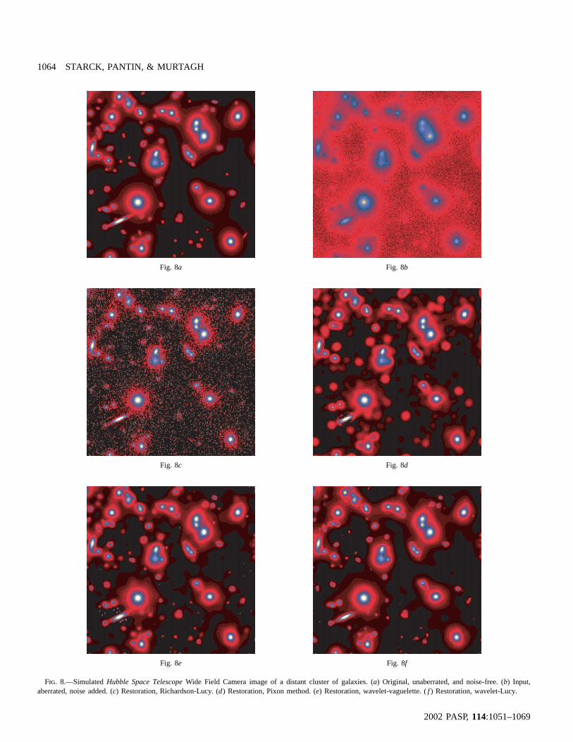
ThePixon method (Dixon et al. 1996; Puetter & Yahil 1999)is relatively different from the previously described methods.This time, an object is modeled as the sum of pseudoimagessmoothed locally by a function with position-dependent scale,called the Pixon shape function. The set of pseudoimages de-fines a dictionary, and the image is supposed to contain onlyfeatures included in this dictionary. But the main problem liesin the fact that features that cannot be detected directly in thedata or in the data after a few Lucy iterations will not bemodeled with the Pixon functions, and they will be stronglyregularized as background. The result is that the faintest objectsare overregularized while strong objects are well restored. Thisis striking in the example shown in Figure 8.

Wavelets offer a mathematical framework for the multi-resolution processing. Furthermore, they furnish an ideal wayto include noise modeling in the deconvolution methods. Sincethe noise is the main problem in deconvolution, wavelets arevery well adapted to the regularization task.

6.3. The Wavelet Transform

We begin with the wavelet transform used in the over-whelming majority of practical applications, for the simple rea-son that its performance in compression is well proven. It isused in the JPEG2000 standard, for instance. Of course, forcompression, it is a nonredundant transform. The schema usedin the wavelet transform output, and the associated frequencydomain tiling, will be familiar to anyone who has studied wave-lets in the nonastronomy (and compression) context. In § 6.4,we will contrast the bi-orthogonal wavelet transform with therecently developed innovative use of the wavelet-vagueletteapproach to noise filtering.

We denote the (bi-) orthogonal wavelet transform andwW

the wavelet transform of a signals, ; w is composedw p Wsof a set of wavelet bands and a coarse version ofs,w cj J

, whereJ is the number of scales usedw p {w , … , w , c }1 J J

in the wavelet transform. Roughly speaking, the Fourier trans-form of a given wavelet band is localized in a frequencywj

band with support , and the Fourier transform ofj�1 j[1/2 , 1/2 ]the smoothed array is localized in the frequency band withcJ


2002 PASP,114:1051–1069

Fig. 3.—Orthogonal wavelet transform representation of an image.

support . Thus, the algorithm outputs subbandJ[0, 1/2 ] J � 1arrays. The indexing is such that, here, corresponds to thej p 1finest scale (high frequencies). Coefficients and are ob-c wj,l j,l

tained by means of the filtersh andg, c p � h(k � 2l)ckj�1,l j,k

and , where the filtersh andg are de-w p � g(k � 2l)ckj�1,l j,k

rived from the analysis wavelet functionw; h and g can beinterpreted as, respectively, a low- and a high-pass filter. An-other important point in this algorithm is the critical sampling.Indeed, the number of pixels in the transformed dataw is equalto the number of pixelsN in the original signal. This is possiblebecause of the decimation performed at each resolution level.The signal at resolution levelj (with pixels and )c N c p sj j 0

is decomposed into two bands and , both of themw cj�1 j�1

containing pixels. Finally, the signals can be reconstructedN /2j

from its wavelet coefficients: , using the inverse�1s p W wwavelet transform.

Figure 2 shows the frequency domain tiling by the one-dimensional wavelet transform. The first convolution step bythe two filtersh andg separates the frequency band into twoparts, the high frequencies and the low frequencies. The firstscale of the wavelet transform corresponds to the high fre-w1

quencies. The same process is then repeated several times onthe low-frequency band, which is separated into two parts ateach step. We get the wavelet scales , …, and . Thew w c2 J J

wavelet transform can be seen as a set of passband filters thathas the properties of being reversible (the original data can bereconstructed from the wavelet coefficients) and nonredundant.

The two-dimensional algorithm is based on separate varia-bles leading to prioritizing of horizontal, vertical, and diagonaldirections. The detail signal is obtained from three wavelets:

the vertical wavelet, the horizontal wavelet, and the diagonalwavelet. This leads to three wavelet subimages at each reso-lution level. This transform is nonredundant, which means thatthe number of pixels in the wavelet-transformed data is thesame as in the input data.

Figure 3 shows the spatial representation of a two-dimen-sional wavelet transform. The first step decomposes the imageinto three wavelet coefficient bands (i.e., horizontal band, ver-tical band, and diagonal band) and the smoothed array. The sameprocess is then repeated on the smoothed array. Figure 4 showsthe wavelet transform of a galaxy (NGC 2997) using four res-olution levels.

Other discrete wavelet transforms exist. The a` trous wavelettransform is very well suited for astronomical data and hasbeen discussed in many papers and books (Starck et al. 1998a).By using the a` trous wavelet transform algorithm, an imageIcan be defined as the sum of itsJ wavelet scales and the lastsmooth array: , where the firstJI(x, y) p c (x, y) � � wjp1J j, x, y

term on the right is the last smoothed array andw denotes awavelet scale. This algorithm is quite different from the pre-vious one. It is redundant; i.e., the number of pixels in thetransformed data is larger than in the input data (each waveletscale has the same size as the original image, hence theredundancy factor is ); and it is isotropic (there are noJ � 1favored orientations). Both properties are useful for the purposeof astronomical image restoration.

Figure 5 shows the a` trous transform of the galaxy NGC2997. Three wavelet scales are shown (upper left, upper right,lower left) and the final smoothed plane (lower right). Theoriginal image is given exactly by the sum of these four images.

Since the wavelet transform is a linear transform, the noisebehavior in wavelet space can be well understood and correctlymodeled. This point is fundamental since one of the main prob-lems of deconvolution is the presence of noise in the data.

6.4. Wavelet-Vaguelette Decomposition

The wavelet-vaguelette decomposition, proposed by Donoho(1995), consists of first applying an inverse filtering:

�1 �1F p P ∗ I � P ∗ N p O � Z, (30)

where is the inverse filter [ ]. The�1 �1ˆ ˆP P (u, v) p 1/P(u, v)noise is not white but remains Gaussian. It is�1Z p P ∗ Namplified when the deconvolution problem is unstable. Thena wavelet transform is applied toF, the wavelet coefficientsare soft- or hard-thresholded (Donoho 1993), and the inversewavelet transform furnishes the solution.

The method has been refined by adapting the wavelet basisto the frequency response of the inverse ofP (Kalifa 1999;Kalifa, Mallat, & Rouge2000). Thismirror wavelet basis hasa time-frequency tiling structure different from conventionalwavelets, and it isolates the frequency where is close to zero,Pbecause a singularity in influences the noise vari-�1P (u , v )s s


2002 PASP,114:1051–1069

Fig. 4.—Galaxy NGC 2997 and its bi-orthogonal wavelet transform.

Fig. 5.—Wavelet transform of NGC 2997 by the a` trous algorithm.

ance in the wavelet scale corresponding to the frequency bandthat includes . Figures 6 and 7 show the decomposition(u , v )s s

of the Fourier space, respectively, in one dimension and twodimensions.

Because it may be not possible to isolate all singularities,Neelamani (1999) and Neelamani, Choi, & Baraniuk (2001)

advocated a hybrid approach, proposing to still use the Fourierdomain so as to restrict excessive noise amplification. Regu-larization in the Fourier domain is carried out with the windowfunction :Wl

2ˆd P(u, v)FW (u, v) p , (31)l 2ˆd P(u, v)F � lT(u, v)

where ,S being the power spectral density2 ˆT(u, v) p j /S(u, v)of the observed signal:

�1 �1F p W ∗ P ∗ I � W ∗ P ∗ N. (32)l l

The regularization parameterl controls the amount of Fourier-domain shrinkage and should be relatively small (!1; Neela-mani et al. 2001). The estimateF still contains some noise,and a wavelet transform is performed to remove the remainingnoise. The optimall is determined using a given cost function.See Neelamani et al. (2001) for more details.

This approach is fast and competitive compared to linearmethods, and the wavelet thresholding removes the Gibbs os-cillations. It presents, however, several drawbacks:

1. The regularization parameter is not so easy to find inpractice (Neelamani et al. 2001) and requires some computationtime, which limits the usefulness of the method.

2. The positivity a priori is not used.3. The power spectrum of the observed signal is generally

not known.4. It is not trivial to consider non-Gaussian noise.


2002 PASP,114:1051–1069

Fig. 6.—Frequency domain tiling using a wavelet packet decompositionwith a mirror basis. The variance of the noise has a hyperbolic growth. Seetext for discussion of the implications of the noise variation.

Fig. 7.—Mirror wavelet basis in two-dimensional space. See text for dis-cussion of the implications of the noise variation.

The second point is important for astronomical images. It iswell known that the positivity constraint has a strong influenceon the solution quality (Kempen & van Vliet 2000). We willsee in the following that it is straightforward to modify thestandard iterative methods in such a way that they benefit fromthe capacity of wavelets to separate the signal from the noise.

6.5. Regularization from the Multiresolution Support

6.5.1. Noise Suppression Based on the Wavelet Transform

We have noted how, in using an iterative deconvolution al-gorithm such as van Cittert or Richardson-Lucy, we define

, the residual at iterationn:(n)R (x, y)

n nR (x, y) p I(x, y) � (P ∗ O )(x, y). (33)

By using the a` trous wavelet transform algorithm, can benRdefined as the sum of itsJ wavelet scales and the last smootharray:

J

nR (x, y) p c (x, y) � w , (34)�J j, x, yjp1

where the first term on the right is the last smoothed array andw denotes a wavelet scale.

The wavelet coefficients provide a mechanism to extract onlythe significant structures from the residuals at each iteration.Normally, a large part of these residuals are statistically non-significant. The significant residual (Murtagh & Starck 1994;Starck & Murtagh 1994) is then

J

nR (x, y) p c � M( j, x, y)w , (35)�J, x, y j, x, yjp1

where is the multiresolution support and is definedM( j, x, y)by

1 if w is significant,j, x, yM( j, x, y) p (36){0 if w is nonsignificant.j, x, y

This describes in a logical or Boolean way if the data containinformation at a given scalej and at a given position .(x, y)Assuming that the noise follows a given distribution,

is significant if the probability that the wavelet coef-w (x, y)j

ficient is due to noise is small [ ]. In theP(d W 1 w d) ! ej, x, y

case of Gaussian noise, is significant if , wherew w 1 kjj, x, y j, x, y j

is the noise standard deviation at scalej andk is a constantjj

generally taken between 3 and 5. Different noise models arediscussed in Starck et al. (1998a). If a priori information isavailable, such as star positions, it can easily be introducedinto the multiresolution support.

An alternative approach was outlined in Murtagh, Starck, &Bijaoui (1995) and Starck, Bijaoui, & Murtagh (1995): thesupport was initialized to zero and built up at each iteration ofthe restoration algorithm. Thus, in equation (35) above,

was additionally indexed byn, the iteration number.M( j, x, y)


2002 PASP,114:1051–1069

In this case, the support was specified in terms of significantpixels at each scale,j; in addition, pixels could become sig-nificant as the iterations proceeded but could not be madenonsignificant.

6.5.2. Regularization of Van Cittert’s Algorithm

Van Cittert’s iteration (van Cittert 1931) is

n�1 n nO (x, y) p O (x, y) � aR (x, y), (37)

with . Regularizationn n nR (x, y) p I (x, y) � (P ∗ O )(x, y)using significant structures leads to

n�1 n n¯O (x, y) p O (x, y) � aR (x, y). (38)

The basic idea of this regularization method consists of de-tecting, at each scale, structures of a given size in the residual

and putting them in the restored image . Then nR (x, y) O (x, y)process finishes when no more structures are detected. Then,we have separated the image into two images˜I(x, y) O(x, y)and ; is the restored image, which ought not to contain˜R(x, y) Oany noise, and is the final residual, which ought not toR(x, y)contain any structure;R is our estimate of the noise .N(x, y)

6.5.3. Regularization of the One-Step Gradient Method

The one-step gradient iteration is

n�1 n ∗ nO (x, y) p O (x, y) � P (x, y) ∗ R (x, y), (39)

with . Regularization byn nR (x, y) p I(x, y) � (P ∗ O )(x, y)significant structures leads to

n�1 n ∗ n¯O (x, y) p O (x, y) � P (x, y) ∗ R (x, y). (40)

6.5.4. Regularization of the Richardson-Lucy Algorithm

From equation (1), we have . Thenn nI (x, y) p (P ∗ O )(x, y), and hencen n nR (x, y) p I(x, y) � I (x, y) I(x, y) p I (x, y) �

.nR (x, y)The Richardson-Lucy equation is

n nI (x, y) � R (x, y)n�1 n ∗O (x, y) p O (x, y) ∗ P (x, y),[ ]nI (x, y)

and regularization leads to

n n¯I (x, y) � R (x, y)n�1 n ∗O (x, y) p O (x, y) ∗ P (x, y).[ ]nI (x, y)

6.5.5. Convergence

The standard deviation of the residual decreases until nomore significant structures are found. Convergence can beestimated from the residual. The algorithm stops when a user-specified threshold is reached:

(j � j )/j ! e. (41)n�1 n nR R R

6.5.6. Examples

A simulatedHubble Space Telescope Wide Field Cameraimage of a distant cluster of galaxies is shown in Figure 8a.The image used was one of a number described in Caulet &Freudling (1993) and Freudling & Caulet (1993). The simulateddata are shown in Figure 8b. Four deconvolution methods weretested: Richardson-Lucy, Pixon, wavelet-vaguelette, and wavelet-Lucy. Deconvolved images are presented, respectively, in Fig-ures 8c, 8d, 8e, and 8f. The Richardson-Lucy method amplifiesthe noise, which implies that the faintest objects disappear inthe deconvolved image. The Pixon method introduces regu-larization, and the noise is under control, while objects where“Pixons” have been detected are relatively well protected fromthe regularization effect. Since the “Pixon” features are detectedfrom noisy partially deconvolved data, the faintest objects arenot in the Pixon map and are strongly regularized. The wavelet-vaguelette method is very fast and produces rela-tively high quality results when compared to Pixon orRichardson-Lucy, but the wavelet-Lucy method seems clearlythe best of the four methods. There are fewer spurious objectsthan in the wavelet-vaguelette method, it is stable for any kindof PSF, and any kind of noise modeling can be considered.

6.6. Wavelet CLEAN

The CLEAN solution is only available if the image does notcontain large-scale structures. Wakker & Schwarz (1988)introduced the concept of multiresolution CLEAN (MRC) inorder to alleviate the difficulties occurring in CLEAN for ex-tended sources. The MRC approach consists of building twointermediate images, the first one (called the smooth map) bysmoothing the data to a lower resolution with a Gaussian func-tion, and the second one (called the difference map) by sub-tracting the smoothed image from the original data. Both ofthese images are then processed separately. By using a standardCLEAN algorithm on them, the smoothed clean map and dif-ference clean map are obtained. The recombination of thesetwo maps gives the clean map at the full resolution. This al-gorithm may be viewed as an artificial recipe, but it has beenshown (Starck et al. 1994, 1998a; Starck & Bijaoui 1994) thatit is linked to multiresolution analysis. Wavelet analysis leadsto a generalization of MRC from a set of scales. The waveletCLEAN (WCLEAN) method consists of the following steps:

1. Apply the wavelet transform to the image: we get .WI


2002 PASP,114:1051–1069

2. Apply the wavelet transform to the PSF: we get .WP

3. Apply the wavelet transform to the CLEAN beam: we get.WC

4. For each scalej of the wavelet transform, apply the CLEANalgorithm using the wavelet scalej of both and .W WI P

5. Apply an iterative reconstruction algorithm using .WC

More details can be found in Starck et al. (1994, 1998a).

6.7. Multiscale Entropy

6.7.1. Introduction

In Starck, Murtagh, & Gastaud (1998b), Starck et al. (2001b),and Starck & Murtagh (1999), the benchmark properties for agood “physical” definition of entropy were discussed, and itwas proposed to consider that the entropy of a signal is thesum of the information at each scale of its wavelet transform(Starck et al. 1998b), and the information of a wavelet coefficientis related to the probability of it being due to noise. Denotinghthe information relative to a single wavelet coefficient, we have

, with , whereJNJ jp1H(X) p � � h(w ) h(w ) p � ln p(w )j kp1 j,k j,k j,k

is the number of scales and is the number of samples (pixels,Nj

time-, or wavelength-interval values) in band (scale)j. ForGaussian noise, the information is proportional to the energyof the wavelet coefficients. The larger the value of a normalizedwavelet coefficient, then the lower will be its probability ofbeing noise and the higher will be the information furnishedby this wavelet coefficient. SinceH is corrupted by the noise,it can be decomposed into two components, one ( ) corre-Hs

sponding to the noncorrupted part and the other ( ) to theHn

corrupted part (Starck et al. 1998b): ;H(X) p H (X) � H (X)s n

is called the signal information and the noise information.H Hs n

For each wavelet coefficient , we have to estimate the pro-wj,k

portions and ofh [with ] thath h h(w ) p h (w ) � h (w )n s j,k n j,k s j,k

should be assigned to and . Hence, signal informationH Hn s

and noise information are defined by

NjJ

H (X) p h (w ),��s s j,kjp1 kp1

NjJ

H (X) p h (w ). (42)��n n j,kjp1 kp1

If a wavelet coefficient is small, its value can be due to noise,and the informationh relative to this single-wavelet coefficientshould be assigned to . More details can be found in StarckHn

et al. (2001b).Following the Bayesian scheme, the functional to minimize

is

NjN J2 2[I � (P ∗ O) ] wk k j,kJ(O) p � a , (43)� ��2 22j 2jkp1 jp1 kp1I j

where is the noise at scalej, is the number of pixels atj Nj j

the scalej, is the noise standard deviation in the data, andjI

J is the number of scales.Rather than minimizing the amount of information in the

solution, we may prefer to minimize the amount of informationthat can be due to the noise. The function is now

N 2[I � (P ∗ O) ]k kJ(O) p � aH (O), (44)� n22jkp1 I

and for Gaussian noise, has been defined byHn

N d w dj j,kJ 1 d w d �uj,kH (X) p u erf du. (45)��n �2 ( )�jjp1 kp1 2jj 0 j

Minimizing can be seen as a kind of adaptive soft-thres-Hn

holding in the wavelet terminology. Finally, equation (44) canbe generalized by (Starck et al. 2001b)

J(O) p H (I � P ∗ O) � aH (O); (46)s n

i.e., we want to minimize the minimum of information due tothe signal in the residual and the minimum of information dueto the noise in the solution.

6.7.2. Example: b Pictoris Image Deconvolution

The b Pictoris image (Pantin & Starck 1996) was obtainedby integrating 5 hr on-source using a mid-infrared camera,TIMMI, placed on the 3.6 ESO telescope (La Silla, Chile). Theraw image has a peak signal-to-noise ratio of 80. It is stronglyblurred by a combination of seeing, diffraction (0�.7 on a 3 mclass telescope), and additive Gaussian noise. The initial diskshape in the original image has been lost after the convolutionwith the PSF (see Fig. 9a). Thus, we need to deconvolve suchan image to get the best information on this object, i.e., theexact profile and thickness of the disk, and subsequently tocompare the results to models of thermal dust emission.

After filtering (see Fig. 9b), the disk appears clearly. Fordetection of faint structures (the disk here), one can calculatethat the application of such a filtering method to this imageprovides a gain of observing time of a factor of around 60.The deconvolved image (Fig. 9c) shows that the disk is ex-tended at 10mm and asymmetrical. The multiscale entropymethod is more effective for regularizing than other standardmethods and leads to good reconstruction of the faintest struc-tures of the dust disk.

6.8. Summary of Scale-based Deconvolution

As already mentioned, our objective in § 6 has been to takethe major categories of deconvolution methods—linear inver-sion, CLEAN, Bayesian optimization, and maximum entropy(respectively, §§ 3, 4, and 5)—and seek where and how res-olution scale information could be incorporated. A key re-quirement for us is that the basic method should stay the same


2002 PASP,114:1051–1069

Fig. 8a Fig. 8b

Fig. 8c Fig. 8d

Fig. 8e Fig. 8f

Fig. 8.—SimulatedHubble Space Telescope Wide Field Camera image of a distant cluster of galaxies. (a) Original, unaberrated, and noise-free. (b) Input,aberrated, noise added. (c) Restoration, Richardson-Lucy. (d) Restoration, Pixon method. (e) Restoration, wavelet-vaguelette. (f ) Restoration, wavelet-Lucy.


2002 PASP,114:1051–1069

in all cases (e.g., well-behaved convergence properties shouldremain well behaved, new artifacts or other degradation mustnot be introduced, and so on). It follows that the essentialproperties of the methods described earlier (e.g., appropriate-ness of particular noise models, use or otherwise of particulara priori assumptions, etc.) hold in the multiple-resolution settingalso. We have cited examples of further reading on theseenhanced methods.

7. DECONVOLUTION AND RESOLUTION

In many cases, there is no sense in trying to deconvolve animage at the resolution of the pixel (especially when the PSFis very large). The idea to limit the resolution is relatively old,because it is already this concept that is used in the CLEANalgorithm (Hogbom 1974). Indeed, the clean beam fixes theresolution in the final solution. This principle was also devel-oped by Lannes & Roques (1987) in a different form. Thisconcept was reinvented, first by Gull & Skilling (1991), whocalled the clean beam theintrinsic correlation function (ICF),and more recently by Magain et al. (1998) and Pijpers (1999).

The ICF is usually a Gaussian, but in some cases it may beuseful to take another function. For example, if we want tocompare two images and , which are obtained with twoI I1 2

wavelengths or with two different instruments, their PSFsP1

and will certainly be different. The classic approach wouldP2

be to deconvolve with and with , so we are sure thatI P I P1 2 2 1

both are at the same resolution. Unfortunately, however, welose some resolution in doing this. Deconvolving both imagesis generally not possible because we can never be sure thatboth solutions and will have the same resolution.O O1 2

A solution would be to deconvolve only the image that hasthe worse resolution (say, ) and to limit the deconvolution toI1

the second image resolution ( ). Then, we just have to takeI2

for the ICF. The deconvolution problem is to find (hidden˜P O2

solution) such that

˜I p P ∗ P ∗ O, (47)1 1 2

and our real solution at the same resolution as is obtainedO I1 2

by convolving with ; and can then be compared.O P O I2 1 2

Introducing an ICFG in the deconvolution equation leadsto just considering a new PSF , which is the convolution of′PP and G. The deconvolution is carried out using , and the′Psolution must be reconvolved withG at the end. In this way,the solution has a constrained resolution, but aliasing may occurduring the iterative process, and it is not sure that the artifactswill disappear after the reconvolution withG. Magain et al.(1998) proposed an innovative alternative to this problem byassuming that the PSF can be considered as the convolutionproduct of two terms, the ICFG and an unknownS:

. UsingS instead ofP in the deconvolution processP p G ∗ Sand a sufficiently large FWHM value forG implies that the

Shannon sampling theorem (Shannon 1948) is never violated.But the problem is now to calculateS, knowingP andG, whichis again a deconvolution problem. Unfortunately, this delicatepoint was not discussed in the original paper. Propagation ofthe error on theS estimation in the final solution has also untilnow not been investigated, even if this issue seems to be quiteimportant.

8. SUPERRESOLUTION

8.1. Definition

Superresolution consists of recovering object spatial fre-quency information outside the spatial bandwidth of the imageformation system. In other terms, frequency components where

have to be recovered. It has been demonstratedP(n) p 0(Donoho et al. 1992) that this is possible under certain con-ditions. The observed object must benearly black, i.e., nearlyzero in all but a small fraction of samples. Denotingn as thenumber of samples,m as the number of nonzero values in theFourier transform of the PSF, and as the incomplete-e p m/nness ratio, it has been shown that an image (Donoho et al.1992):

1. Must admit superresolution if the object is -black.1e2

2. Might admit superresolution if the object ise-black. Inthis case, it depends on the noise level and the spacing ofnonzero elements in the object. Well-spaced elements favor thepossibility of superresolution.

3. Cannot admit superresolution if the object is note-black.

Near-blackness is both necessary and sufficient for super-resolution. Astronomical images often give rise to such datasets, where the real information (stars and galaxies) is containedin very few pixels. If the -blackness of the object is not1e2

verified, a solution is to limit the Fourier domainQ of therestored object. Several methods have been proposed in dif-ferent contexts for achieving superresolution.

8.2. Gerchberg-Saxon-Papoulis Method

The Gerchberg-Saxon-Papoulis (Gerchberg 1974) method isiterative and uses the a priori information on the object, whichis its positivity and its support in the spatial domain. It wasdeveloped for interferometric image reconstruction, where wewant to recover the objectO from some of itsvisibilities, i.e.,some of its frequency components. Hence, the object is sup-posed to be known in a given Fourier domainQ, and we needto recover the object outside this domain. The problem canalso be seen as a deconvolution problem , whereI p P ∗ O

1 if (u, v) � Q,P(u, v) p (48){0 otherwise.

We denote and the projection operators in the spatialP PC Cs f


2002 PASP,114:1051–1069

Fig. 9a Fig. 9b

Fig. 9c

Fig. 9.—(a) b Pictoris raw data; (b) filtered image; (c) deconvolved image.

and the Fourier domain:

X(x, y) if ( x, y) � D,P (X(x, y)) p (49)Cs {0 otherwise;

Î(u, v) p O(u, v) if (u, v) � Q,ˆP (X(u, v)) pC ˆf { X(u, v) otherwise.

The projection operator replaces by zero all pixel valuesPCs

that are not in the spatial support defined by , and replacesD PCf

all frequencies in the Fourier domainQ by the frequencies ofthe objectO. The Gerchberg algorithm is as follows:

1. Compute p inverse Fourier transform of , and set0˜ Ô I.i p 0

2. Compute .i˜X p P (O )1 Cs

3. Compute p Fourier transform of .X X1 1

4. Compute .ˆ ˆX p P (X )2 C 1f

5. Compute p inverse Fourier transform of .ˆX X2 2

6. Compute .i�1˜ Ô p P (X )C 2s

7. Set , , and go to 2.i�1˜X p O i p i � 11

The algorithm consists just of forcing iteratively the solutionto be zero outside the spatial domain and equal to the ob-D

served visibilities inside the Fourier domainQ. It has been


2002 PASP,114:1051–1069

shown that this algorithm can be derived from the Landwebermethod (Bertero & Boccacci 1998), and therefore its conver-gence and regularization properties are the same as for theLandweber method. It is straightforward to introduce the pos-itivity constraint by replacing by :�P PC Cs s

max (X(x, y),0) if (x, y) � D,�P (X(x, y)) p (50)Cs {0 otherwise.

The Gerchberg method can be generalized (Bertero & Boc-cacci 1998) using the Landweber iteration:

n�1 � n ∗ ∗ nO p P [O � a(P ∗ L � P ∗ P ∗ O )], (51)Cs

where .�L p P (I)Cs

8.3. Deconvolution with Interpolation

The MAP Poisson algorithm, combined with an interpola-tion, can be used to achieve superresolution (Hunt 1994):

In�1 n ∗O p O exp � 1 ∗ P , (52)F( ){ }n(P ∗ O )f

where up-arrow and down-arrow notation describes, respec-tively, the oversampling and downsampling operators. The PSFP must be sampled on the same grid as the object.

8.4. Undersampled PSF

When considering sampling, we should remember that de-tector pixels are “bins” for capturing flux and hence that thereis inherent area integration. At all times, therefore, signal de-tection implies signal convolution. Passing from one spatialresolution to another (which is implicit, for example, whencross-correlating signals from different detectors) necessarilyinvolves deconvolution, however this is actually achieved inpractice.

We now look at the case where observations are made withan undersampled PSF. When the observation is repeated severaltimes with a small shift between two measurements, we canreconstruct a deconvolved image on a smaller grid. We denote

the kth observation ( …,n), , the shiftD(i, j, k) k p 1 D Di,k j,k

in both directions relative to the first frame, the operatorLF

that co-adds all the frame on a smaller grid, and the operator�1Lf

that estimatesD from using shifting and downsamplingL DF

operations. The , shifts are generally derived from theD Di,k j,k

observations using correlation methods or a PSF fitting (if astar is in the field) but can also be the jitter information if thedata are obtained from space. Note also that . The�1L L D ( Df F

PSFP can generally be derived on a finer grid using a set ofobservations of a star or using an optical modeling of the

instrument. The deconvolution iteration becomes

n�1 n ∗ �1 nO p O � aP [L (D � L (P ∗ O ))] (53)F f

and the positivity and spatial constraints can also be used:

n�1 � n ∗ �1 nO p P {O � aP [L (D � L (P ∗ O ))]}. (54)C F fs

The co-addition operator can be implemented in differentLF

ways. All frames can first be interpolated to the finer grid size,shifted using an interpolation function, and then co-added.

“Dithering” or “jitter” have been terms applied to purposefuluse of offsets in imaging (Hook & Fruchter 2000). An ad-hocmethod called “drizzling” was developed by Hook & Fruchter(2000) and implemented in IRAF, based on mapping pixels toa finer grid and assuming knowledge of geometric distortion.

Dithering may be described as a way of recovering Nyquistsampling. Moving the source image to get new samples is easyto understand, particularly with the effective PSF concept,where the effective PSF combines the native optical PSF andthe areal integral within the detector. In recent work, Gam-maitoni et al. (1998) consider dithering as a special case of“stochastic resonance,” which in general seeks to amplify weaksignals by the assistance of small quantities of noise.

Lauer (1999) ignores geometric distortion and instead ad-dresses the problem of aliasing resulting from combiningundersampled images. A linear combination of Fourier trans-forms of the offset images is used, which mitigates aliasingartifacts in direct space.

8.5. Multiscale Support Constraint

The constraint operator may not always be easy to de-�PCs

termine, especially when the observed object is extended. Fur-thermore, if the object is very extended, the support will bevery large and the support constraint may have very smallinfluence on the final result. For this reason, it may be con-venient to replace the support constraint by the multiresolutionsupport constraint. The advantages are the following:

1. It can be automatically calculated from the noise modelingin the wavelet space.

2. Extended objects are generally also smooth. This meansthat the support on the small scales will be small, and thereforethis introduces a smoothness constraint on extended objectsand no constraint on pointlike objects.

9. CONCLUSIONS

We conclude with a short look at how multiscale methodsused in deconvolution are evolving and maturing.

We have seen that the recent improvement in deconvolutionmethods has led to use of multiscale approaches. These can besummarized as follows:


2002 PASP,114:1051–1069

1. Linear inverse filtering leading to wavelet-vaguelettedecomposition.

2. CLEAN leading to wavelet-CLEAN.3. Fixed-step gradient, Lucy, and van Cittert leading to reg-

ularization by the multiresolution support.4. MEM leading to the multiscale entropy method.

The multiscale entropy method (Starck et al. 2001b), whichgeneralized the wavelet-regularized iterative methods, allowsus to separate the deconvolution problem into two separateproblems: noise control from one side and solution smoothnesscontrol on the other side. The advantage of this approach isthat noise control is better carried out in the image domain,while smoothness control can only be carried out in the objectdomain.

The success of wavelets is due to the fact that wavelet basesrepresent well a large class of signals. Other multiscale meth-ods, such as the ridgelet or the curvelet transform (Cande`s &Donoho 1999, 2000; Donoho & Duncan 2000; Starck, Cande`s,& Donoho 2001a) will certainly play a role in the future.

An old view of astronomy in practice is that of the obser-vational specialist, aided by one or more data-analysis spe-cialists. This view is changing fast with the coming of astron-omy “collaboratories” supported by middleware and Webservices. Our review of deconvolution is addressed to the teamsthat are leading the evolution toward use of the Grid and“virtual observatory.”

The virtual observatory in astronomy is premised on the factthat all usable astronomy data are digital. High-performanceinformation cross-correlation and fusion, and long-term avail-ability of information, are required. The term “virtual” in thiscontext means the use of reduced or processed on-line data.

A second and closely associated development is that of theGrid. The computational Grid is to provide an algorithmic andprocessing infrastructure for the virtual science of the future.The data Grid is to allow ready access to information from ourtera- and petabyte data stores. The information Grid is toprovide active and dynamic retrieval of information, not justpointers to where information might or might not exist.

The evolution of the way we do science, driven by thesethemes, is inextricably linked to the problem areas and oftenrecently developed algorithmic solutions surveyed in thisarticle.

As just one location for further information on innovativedevelopments in this broad area, see “Computational andInformation Infrastructure in the Astronomical DataGrid” onthe iAstro Web site.2 This is a 4 year (from late 2001) Europeancollaborative project.

We are grateful to an anonymous referee for various com-ments on an earlier version of this article.

2 http://www.iAstro.org.

REFERENCES

Acar, R., & Vogel, C. 1994, Physica D, 10, 1217Adorf, H., Hook, R., & Lucy, L. 1995, Int. J. Imaging Syst. Tech.,

6, 339Alloin, D., Pantin, E., Lagage, P. O., & Granato, G. L. 2000, A&A,

363, 926Alvarez, L., Lions, P.-L., & Morel, J.-M. 1992, SIAM J. Numer. Anal.,

29, 845Bertero, M., & Boccacci, P. 1998, Introduction to Inverse Problems

in Imaging (London: Inst. Phys.)Blanc-Feraud, L., & Barlaud, M. 1996, Vistas Astron., 40, 531Bontekoe, T., Koper, E., & Kester, D. 1994, A&A, 284, 1037Buonanno, R., Buscema, G., Corsi, C., Ferraro, I., & Iannicola, G.

1983, A&A, 126, 278Burg, J. 1978, in Modern Spectral Analysis, ed. D. G. Childers (New

York: IEEE Press), 34Burud, I., et al. 2002, A&A, 383, 71Candes, E. & Donoho, D. 1999, Philos. Trans. R. Soc. London A,

357, 2495———. 2000, Proc. SPIE, 4119, 1Caulet, A., & Freudling, W. 1993, ST-ECF Newsl., 20, 5Champagnat, F., Goussard, Y., & Idier, J. 1996, IEEE Trans. Image

Process., 44, 2988Charbonnier, P., Blanc-Fe´raud, L., Aubert, G., & Barlaud, M. 1997,

IEEE Trans. Image Process., 6, 298Christou, J. C., Bonnacini, D., Ageorges, N., & Marchis, F. 1999,

Messenger, 97, 14

Corbard, T., Blanc-Fe´raud, L., Berthomieu, G., & Provost, J. 1999,A&A, 344, 696

Cornwell, T. 1989, in Diffraction-Limited Imaging with Very LargeTelescopes, ed. D. Alloin & J. Mariotti (Dordrecht: Kluwer), 273

Courbin, F., Lidman, C., & Magain, P. 1998, A&A, 330, 57Coustenis, A., et al. 2001, Icarus, 154, 501Dempster, A., Laird, N., & Rubin, D. 1977, J. Royal Stat. Soc. B, 39, 1Dixon, D., et al. 1996, A&AS, 120, 683Djorgovski, S. 1983, J. Astrophys. Astron., 4, 271Donoho, D. 1993, in Proc. Symp. Applied Mathematics 47, Different

Perspectives on Wavelets, ed. I. Daubechies (Providence: Am.Math. Soc.), 173

———. 1995, Appl. Comput. Harmonic Anal., 2, 101Donoho, D., & Duncan, M. 2000, Proc. SPIE, 4056, 12Donoho, D., Johnson, I., Hoch, J., & Stern, A. 1992, J. Royal Stat.

Soc. B, 54, 41Faure, C., Courbin, F., Kneib, J. P., Alloin, D., Bolzonella, M., &

Burud, I. 2002, A&A, 386, 69Freudling, W., & Caulet, A. 1993, in Proc. 5th ESO/ST-ECF Data

Analysis Workshop, ed. P. Grosbøl (Garching: ESO), 63Frieden, B. 1978, Image Enhancement and Restoration (Berlin:

Springer)Galatsanos, N., & Katsaggelos, A. 1992, IEEE Trans. Image Process.,

1, 322Gammaitoni, L., Ha¨nggi, P., Jung, P., & Marchesoni, F. 1998, Rev.

Mod. Phys., 70, 223Gerchberg, R. 1974, Opt. Acta, 21, 709


2002 PASP,114:1051–1069

Golub, G., Heath, M., & Wahba, G. 1979, Technometrics, 21, 215Gull, S., & Skilling, J. 1991, MEMSYS5 Quantified Maximum

Entropy User’s Manual (Suffolk: Maximum Entropy DataConsultants)

Hanisch, R. J. & White, R. L., eds. 1994, Proc. STScI Workshop, TheRestoration of HST Images and Spectra II (Baltimore: STScI)

Hogbom, J. 1974, A&AS, 15, 417Hook, R. 1999, ST-ECF Newsl., 26, 3Hook, R., & Fruchter, A. 2000, in ASP Conf. Ser. 216, Astronomical

Data Analysis Software and Systems IX, ed. N. Manset, C. Veillet,& D. Crabtree (San Francisco: ASP), 521

Hunt, B. 1994, Int. J. Mod. Phys. C, 5, 151Issacson, E., & Keller, H. 1966, Analysis of Numerical Methods (New

York: Wiley)Kaaresen, K. 1997, IEEE Trans. Image Process., 45, 1173Kalifa, J. 1999, Ph.D. thesis, Ecole PolytechniqueKalifa, J., Mallat, S., & Rouge´, B. 2000, IEEE Trans. Image Process.,

submittedKatsaggelos, A. 1993, Digital Image Processing (Berlin: Springer)Kempen, G., & van Vliet, L. 2000, J. Opt. Soc. Am. A, 17, 425Landweber, L. 1951, Am. J. Math., 73, 615Lannes, A., & Roques, S. 1987, J. Opt. Soc. Am., 4, 189Lauer, T. 1999, PASP, 111, 227Lucy, L. 1974, AJ, 79, 745———. 1994, in The Restoration of HST Images and Spectra II, ed.

R. J. Hanisch & R. L. White (Boston: STScI), 79Magain, P., Courbin, F., & Sohy, S. 1998, ApJ, 494, 472Marchis, R., Prange´, R., & Christou, J. 2000, Icarus, 148, 384Moffat, A. 1969, A&A, 3, 455Molina, R., & Cortijo, F. 1992, in Proc. International Conference on

Pattern Recognition, ed. E. S. Gelsema & E. Backer (Vol. 3; LosAlamitos: IEEE IEEE Comp. Soc.), 147

Molina, R., Katsaggelos, A., Mateos, J., & Abad, J. 1996, VistasAstron., 40, 539

Molina, R., Katsaggelos, A., Mateos, J., Hermoso, A., & Segall, A.2000, Pattern Recognition, 33, 555

Molina, R., Nunez, J., Cortijo, F., & Mateos, J. 2001, IEEE SignalProcess. Magazine, 18, 11

Molina, R., Ripley, B., Molina, A., Moreno, F., & Ortiz, J. 1992, AJ,104, 1662

Murtagh, F., & Starck, J. 1994, ST-ECF Newsl., 21, 19Murtagh, F., Starck, J., & Bijaoui, A. 1995, A&AS, 112, 179Neelamani, R. 1999, M.S. thesis, Rice Univ.Neelamani, R., Choi, H., & Baraniuk, R. G. 2001, IEEE Trans. Image

Process., submitted

Nunez, J., & Llacer, J. 1998, A&AS, 131, 167Pantin, E., & Starck, J. 1996, A&AS, 118, 575Perona, P. & Malik, J. 1990, IEEE Trans. Pattern Analysis and Ma-

chine Intelligence, 12, 629Pijpers, F. P. 1999, MNRAS, 307, 659Pirzkal, N., Hook, R., & Lucy, L. 2000, in ASP Conf. Ser. 216,

Astronomical Data Analysis Software and Systems IX, ed. N. Man-set, C. Veillet, & D. Crabtree (San Francisco: ASP), 655

Puetter, R., & Yahil, A. 1999, in ASP Conf. Ser. 172, AstronomicalData Analysis Software and Systems VIII, ed. D. M. Mehringer,R. L. Plante, & D. A. Roberts (San Francisco: ASP), 307

Radomski, J. T., Pinã, R. K., Packham, C., Telesco, C. M., & Tad-hunter, C. N. 2002, ApJ, 566, 675

Richardson, W. 1972, J. Opt. Soc. Am., 62, 55Ripley, B. 1981, Spatial Statistics (New York: Wiley)Rudin, L., Osher, S., & Fatemi, E. 1992, Physica D, 60, 259Shannon, C. 1948, Bell Syst. Tech. J., 27, 379Shepp, L., & Vardi, Y. 1982, IEEE Trans. Medical Imaging, 2, 113Starck, J., & Bijaoui, A. 1994, Signal Process., 35, 195Starck, J., Bijaoui, A., Lopez, B., & Perrier, C. 1994, A&A, 283, 349Starck, J., Bijaoui, A., & Murtagh, F. 1995, CVGIP: Graphical Models

& Image Processing, 57, 420Starck, J., Cande`s, E., & Donoho, D. 2001a, IEEE Trans. Image Pro-

cess., 11, 670Starck, J., & Murtagh, F. 1994, A&A, 288, 342———. 1999, Signal Process., 76, 147———. 2002, Astronomical Image and Data Analysis (Berlin:

Springer), in pressStarck, J., Murtagh, F., & Bijaoui, A. 1998a, Image Processing and

Data Analysis: The Multiscale Approach (Cambridge: CambridgeUniv. Press)

Starck, J., Murtagh, F., & Gastaud, R. 1998b, IEEE Trans. on Circuitsand Systems II, 45, 1118

Starck, J., Murtagh, F., Querre, P., & Bonnarel, F. 2001b, A&A, 368,730

Tikhonov, A., Goncharski, A., Stepanov, V., & Kochikov, I. 1987,Sov. Phys.–Doklady, 32, 456

van Cittert, P. 1931, Z. Phys., 69, 298Wakker, B., & Schwarz, U. 1988, A&A, 200, 312Weir, N. 1992, in ASP Conf. Ser. 25, Astronomical Data Analysis,

Software, and Systems I, ed. D. Worral, C. Biemesderfer, & J.Barnes (San Francisco: ASP), 186

White, R. L., & Allen, R. J., eds. 1990, Proc. STScI Workshop, TheRestoration of HST Images and Spectra (Baltimore: STScI)

Zavagno, A., Lagage, P. O., & Cabrit, S. 1999, A&A, 344, 499

Documents

Review - Jean-Luc Starckjstarck.free.fr/pasp02.pdf · 1052 STARCK, PANTIN, & MURTAGH 2002 PASP, 114:1051–1069 Fig. 1.—Active galactic nucleus of NGC 1068 observed at 20 mm. Left: