Review

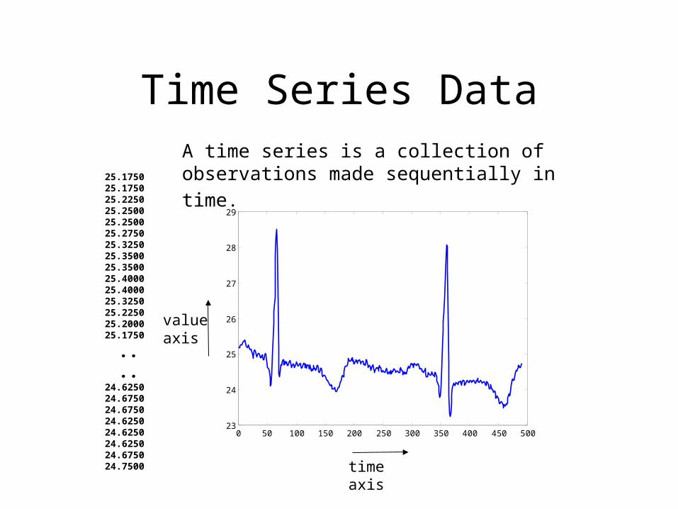
Time Series Data

0 50 100 150 200 250 300 350 400 450 50023

24

25

26

27

28

29

25.1750 25.1750 25.2250 25.2500 25.2500 25.2750 25.3250 25.3500 25.3500 25.4000 25.4000 25.3250 25.2250 25.2000 25.1750

.. .. 24.6250 24.6750 24.6750 24.6250 24.6250 24.6250 24.6750 24.7500

A time series is a collection of observations

made sequentially in time.

time axis

valueaxis

Time Series Problems (from a databases perspective)

• The Similarity Problem

X = x1, x2, …, xn and Y = y1, y2, …, yn

• Define and compute Sim(X, Y)– E.g. do stocks X and Y have similar movements?

• Retrieve efficiently similar time series (Similarity Queries)

Similarity Models

• Euclidean and Lp based• Dynamic Time Warping• Edit Distance and LCS based• Probabilistic (using Markov Models)• Landmarks

• How appropriate a similarity model is depends on the application

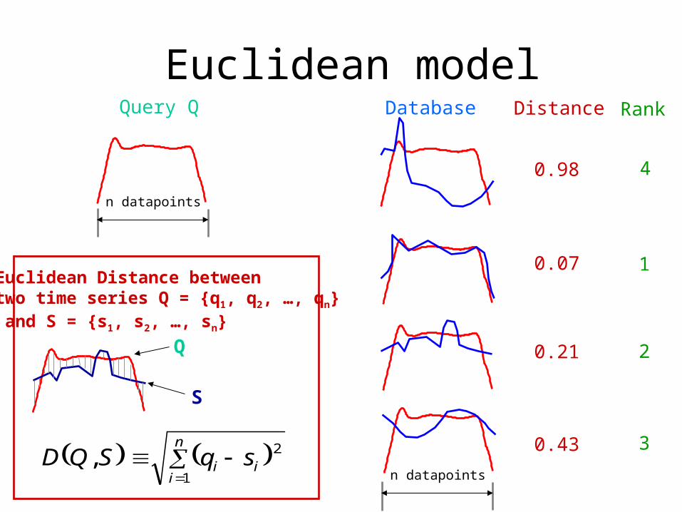
Euclidean modelQuery Q

n datapoints

n

iii sqSQD

1

2,

S

Q

Euclidean Distance betweentwo time series Q = {q1, q2, …, qn} and S = {s1, s2, …, sn}

Distance

0.98

0.07

0.21

0.43

Rank

4

1

2

3

Database

n datapoints

Dynamic Time Warping[Berndt, Clifford, 1994]

• Allows acceleration-deceleration of signals along the time dimension

• Basic idea

– Consider X = x1, x2, …, xn , and Y = y1, y2, …, yn

– We are allowed to extend each sequence by repeating elements

– Euclidean distance now calculated between the extended sequences X’ and Y’

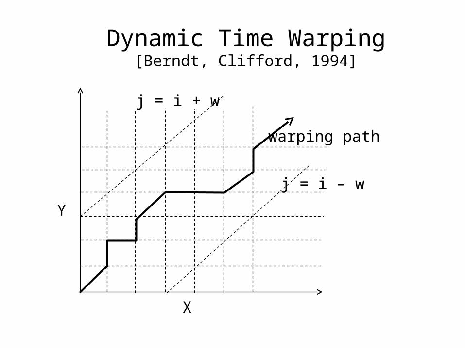
X

Y

warping path

j = i – w

j = i + w

Dynamic Time Warping[Berndt, Clifford, 1994]

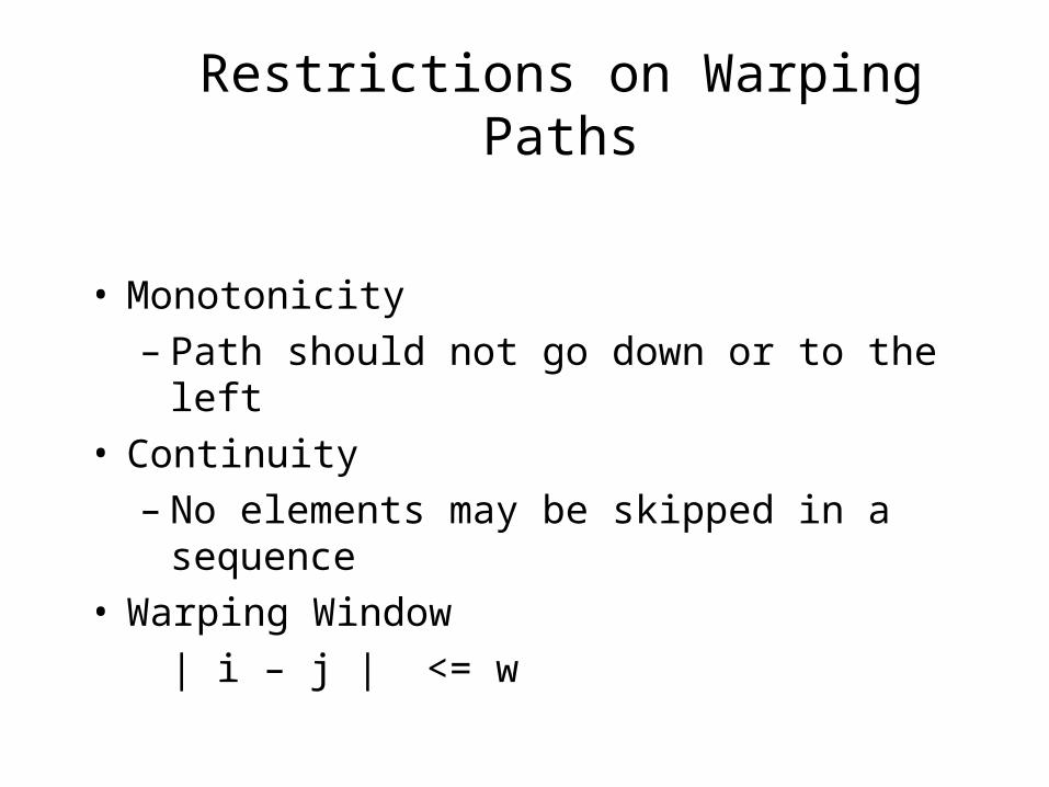
Restrictions on Warping Paths

• Monotonicity– Path should not go down or to the left

• Continuity– No elements may be skipped in a sequence

• Warping Window

| i – j | <= w

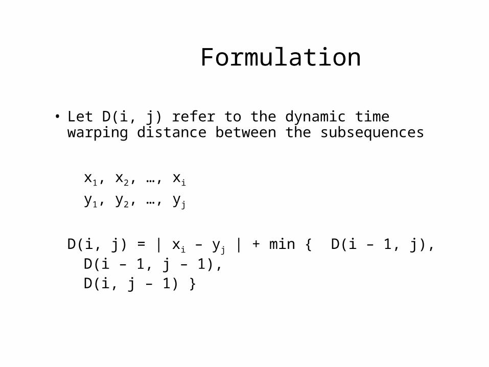
Formulation

• Let D(i, j) refer to the dynamic time warping distance between the subsequences

x1, x2, …, xi

y1, y2, …, yj

D(i, j) = | xi – yj | + min { D(i – 1, j), D(i – 1, j – 1), D(i, j – 1) }

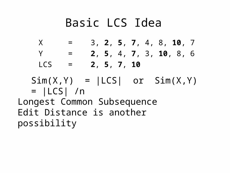
Basic LCS Idea

X = 3, 2, 5, 7, 4, 8, 10, 7

Y = 2, 5, 4, 7, 3, 10, 8, 6

LCS = 2, 5, 7, 10

Sim(X,Y) = |LCS| or Sim(X,Y) = |LCS| /n

Longest Common SubsequenceEdit Distance is another possibility

Indexing Time Series using ‘GEMINI’

(GEneric Multimedia INdexIng)

Extract a few numerical features, for a ‘quick and dirty’ test

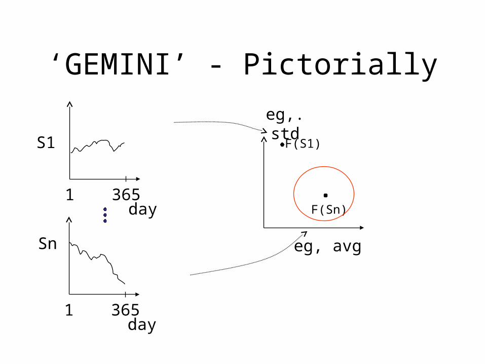
day1 365

day1 365

S1

Sn

F(S1)

F(Sn)

‘GEMINI’ - Pictorially

eg, avg

eg,. std

GEMINI

Solution: Quick-and-dirty' filter:

• extract n features (numbers, eg., avg., etc.)

• map into a point in n-d feature space

• organize points with off-the-shelf spatial access method (‘SAM’)

• discard false alarms

GEMINI

Important: Q: how to guarantee no false dismissals?

A1: preserve distances (but: difficult/impossible)

A2: Lower-bounding lemma: if the mapping ‘makes things look closer’, then there are no false dismissals

Feature Extraction

• How to extract the features? How to define the feature space?

• Fourier transform

• Wavelets transform

• Averages of segments (Histograms or APCA)

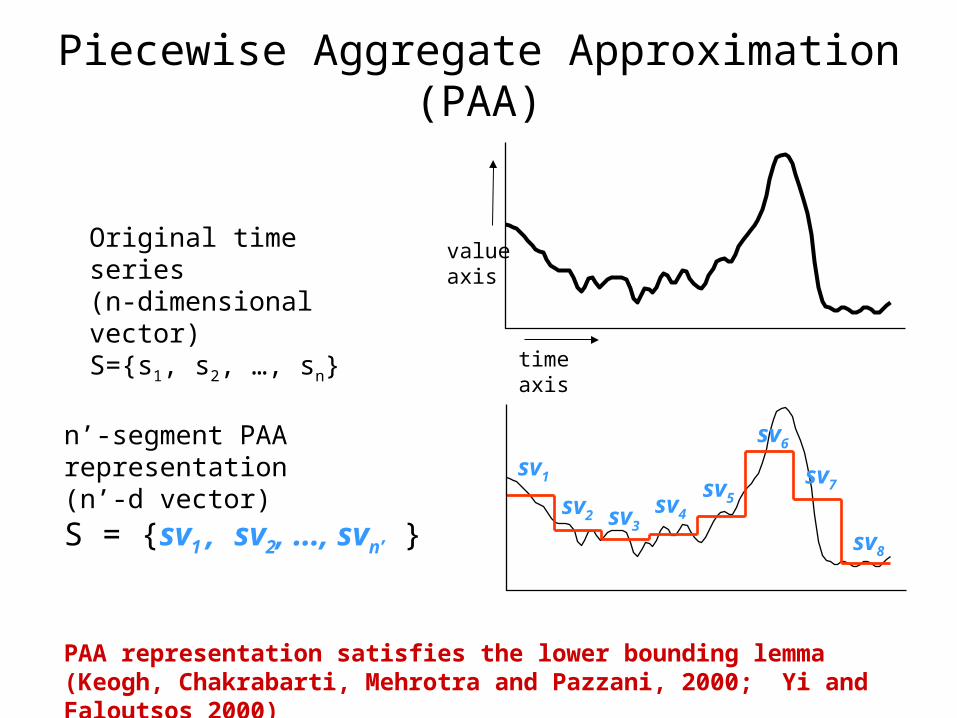
Piecewise Aggregate Approximation (PAA)

valueaxis

time axis

Original time series(n-dimensional vector)S={s1, s2, …, sn}

n’-segment PAA representation (n’-d vector)

S = {sv1 , sv2, …, svn’ }sv1

sv2 sv3sv4

sv5

sv6

sv7

sv8

PAA representation satisfies the lower bounding lemma(Keogh, Chakrabarti, Mehrotra and Pazzani, 2000; Yi and Faloutsos 2000)

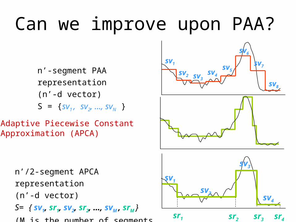
Can we improve upon PAA?

n’-segment PAA representation

(n’-d vector)

S = {sv1 , sv2, …, svN }

sv1

sv2 sv3sv4

sv5

sv6

sv7

sv8

sv1

sv2

sv3

sv4

sr1 sr2 sr3 sr4

n’/2-segment APCA representation

(n’-d vector)

S= { sv1, sr1, sv2, sr2, …, svM , srM }

(M is the number of segments = n’/2)

Adaptive Piecewise Constant Approximation (APCA)

Dimensionality Reduction

• Many problems (like time-series and image similarity) can be expressed as proximity problems in a high dimensional space

• Given a query point we try to find the points that are close…

• But in high-dimensional spaces things are different!

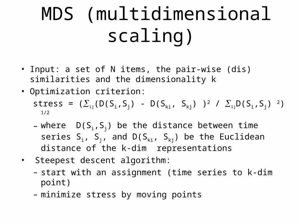
MDS (multidimensional scaling)

• Input: a set of N items, the pair-wise (dis) similarities and the dimensionality k

• Optimization criterion:

stress = (ij(D(Si,Sj) - D(Ski, Skj) )2 / ijD(Si,Sj) 2) 1/2

– where D(Si,Sj) be the distance between time series Si, Sj, and D(Ski, Skj) be the Euclidean distance of the k-dim representations

• Steepest descent algorithm:

– start with an assignment (time series to k-dim point)

– minimize stress by moving points

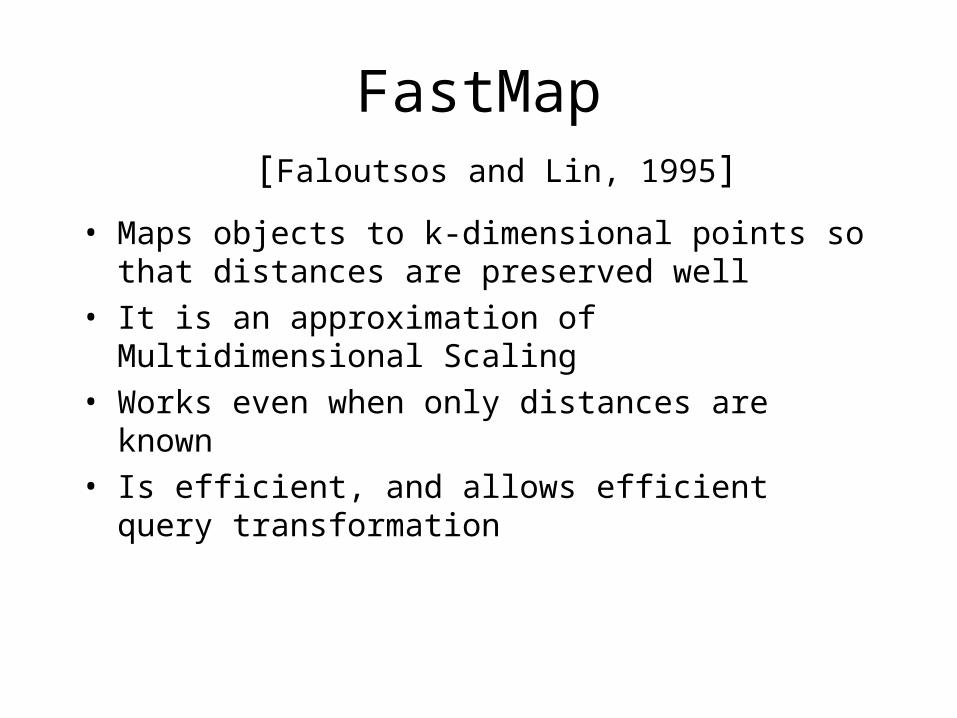
FastMap [Faloutsos and Lin, 1995]

• Maps objects to k-dimensional points so that distances are preserved well

• It is an approximation of Multidimensional Scaling

• Works even when only distances are known

• Is efficient, and allows efficient query transformation

Other DR methods

• PCA (Principle Component Analysis)

Move the center of the dataset to the center of the origins. Define the covariance matrix ATA. Use SVD and project the items on the first k eigenvectors

• Random projections

What is Data Mining?

• Data Mining is:(1) The efficient discovery of previously

unknown, valid, potentially useful, understandable patterns in large datasets

(2) The analysis of (often large) observational data sets to find unsuspected relationships and to summarize the data in novel ways that are both understandable and useful to the data owner

What is Data Mining?

• Data Mining is:(1) The efficient discovery of previously

unknown, valid, potentially useful, understandable patterns in large datasets

(2) The analysis of (often large) observational data sets to find unsuspected relationships and to summarize the data in novel ways that are both understandable and useful to the data owner

Association Rules• Given: (1) database of transactions, (2) each transaction is

a list of items (purchased by a customer in a visit)• Find: all association rules that satisfy user-specified

minimum support and minimum confidence interval• Example: 30% of transactions that contain beer also

contain diapers; 5% of transactions contain these items– 30%: confidence of the rule– 5%: support of the rule

• We are interested in finding all rules rather than verifying if a rule holds

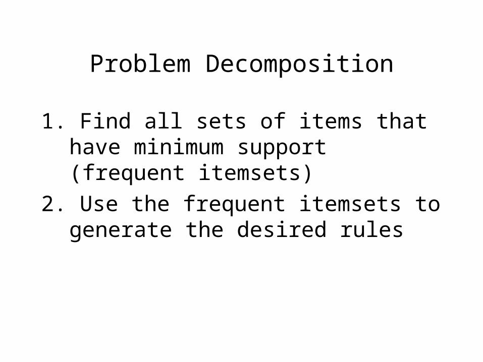
Problem Decomposition

1. Find all sets of items that have minimum support (frequent itemsets)

2. Use the frequent itemsets to generate the desired rules

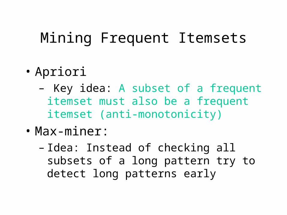
Mining Frequent Itemsets

• Apriori– Key idea: A subset of a frequent itemset must

also be a frequent itemset (anti-monotonicity)

• Max-miner:– Idea: Instead of checking all subsets of a long

pattern try to detect long patterns early

FP-tree

• Compress a large database into a compact, Frequent-Pattern tree (FP-tree) structure– highly condensed, but complete for frequent

pattern mining

• Create the tree and then run recursively the algorithm over the tree (conditional base for each item)

Association Rules

• Multi-level association rules: each attribute has a hierarchy. Find rules per level or at different levels

• Quantitative association rules– Numerical attributes

• Other methods to find correlation:– Lift, correlation coefficient

)()(

)(, BPAP

BAPcorr BA

Major Clustering Approaches

• Partitioning algorithms: Construct various partitions and then

evaluate them by some criterion

• Hierarchical algorithms: Create a hierarchical decomposition of

the set of data (or objects) using some criterion

• Density-based algorithms: based on connectivity and density

functions

• Model-based: A model is hypothesized for each of the clusters

and the idea is to find the best fit of that model to each other

Partitioning Algorithms: Basic Concept

• Partitioning method: Construct a partition of a database D of n objects into a set of k clusters

• Given a k, find a partition of k clusters that optimizes the chosen partitioning criterion

– Global optimal: exhaustively enumerate all partitions

– Heuristic methods: k-means and k-medoids algorithms

– k-means (MacQueen’67): Each cluster is represented by the center of the cluster

– k-medoids or PAM (Partition around medoids) (Kaufman & Rousseeuw’87): Each cluster is represented by one of the objects in the cluster

Optimization problem

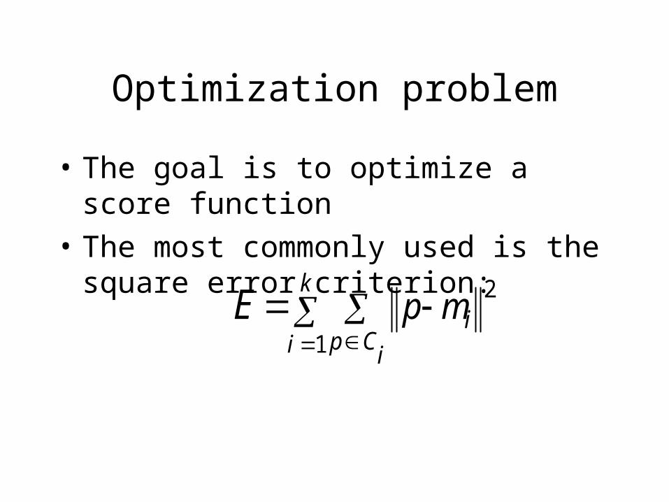
• The goal is to optimize a score function

• The most commonly used is the square error criterion:

k

i iCp

impE1

2

CLARANS (“Randomized” CLARA)

• CLARANS (A Clustering Algorithm based on Randomized Search) (Ng and Han’94)

• CLARANS draws sample of neighbors dynamically

• The clustering process can be presented as searching a graph where every node is a potential solution, that is, a set of k medoids

• If the local optimum is found, CLARANS starts with new randomly selected node in search for a new local optimum

• It is more efficient and scalable than both PAM and CLARA

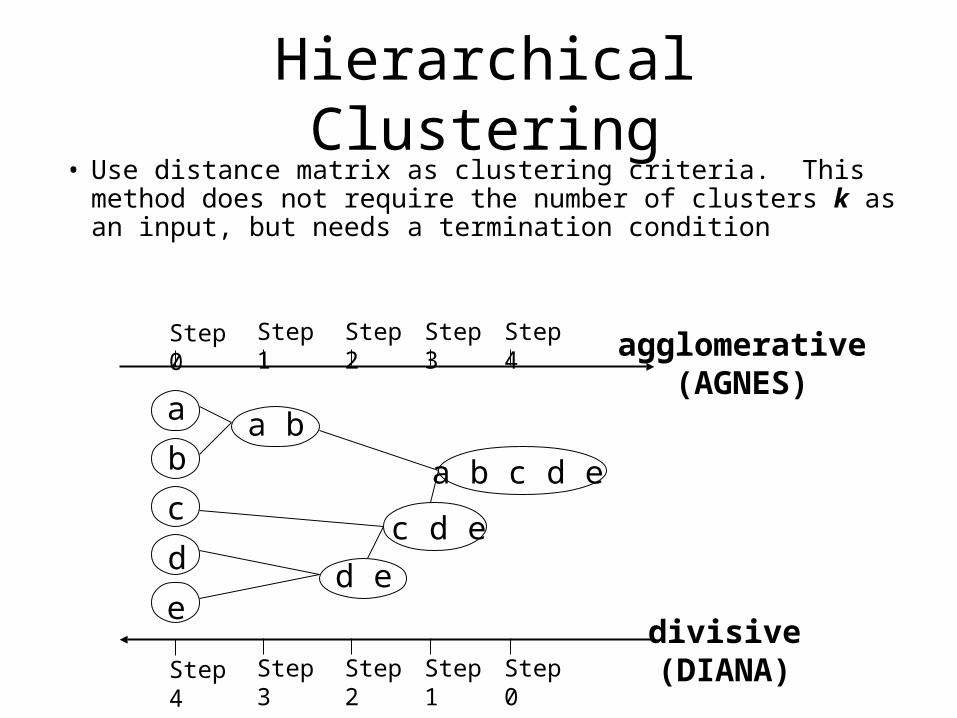
Hierarchical Clustering• Use distance matrix as clustering criteria. This method does

not require the number of clusters k as an input, but needs a termination condition

Step 0 Step 1 Step 2 Step 3 Step 4

b

d

c

e

a a b

d e

c d e

a b c d e

Step 4 Step 3 Step 2 Step 1 Step 0

agglomerative(AGNES)

divisive(DIANA)

HAC

• Different approaches to merge clusters:– Min distance– Average distance– Max distance– Distance of the centers

BIRCH • Birch: Balanced Iterative Reducing and Clustering using

Hierarchies, by Zhang, Ramakrishnan, Livny (SIGMOD’96)

• Incrementally construct a CF (Clustering Feature) tree, a hierarchical data structure for multiphase clustering

– Phase 1: scan DB to build an initial in-memory CF tree (a multi-level compression of the data that tries to preserve the inherent clustering structure of the data)

– Phase 2: use an arbitrary clustering algorithm to cluster the leaf nodes of the CF-tree

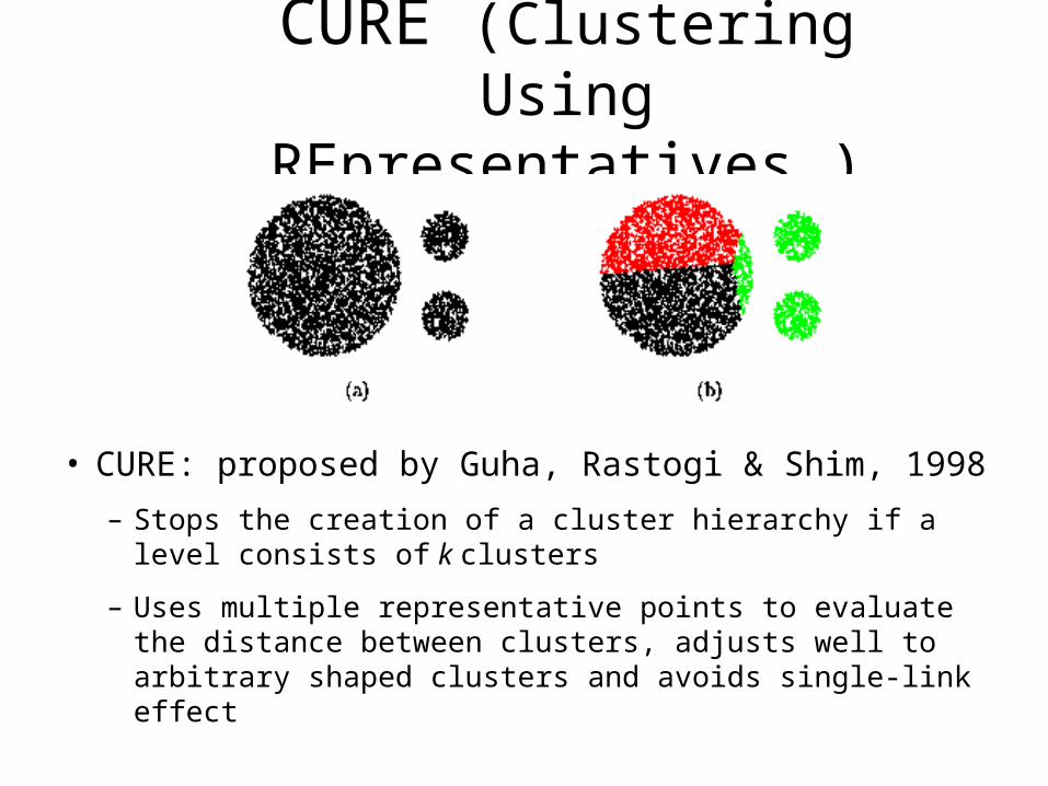
CURE (Clustering Using REpresentatives )

• CURE: proposed by Guha, Rastogi & Shim, 1998

– Stops the creation of a cluster hierarchy if a level consists of k clusters

– Uses multiple representative points to evaluate the distance between clusters, adjusts well to arbitrary shaped clusters and avoids single-link effect

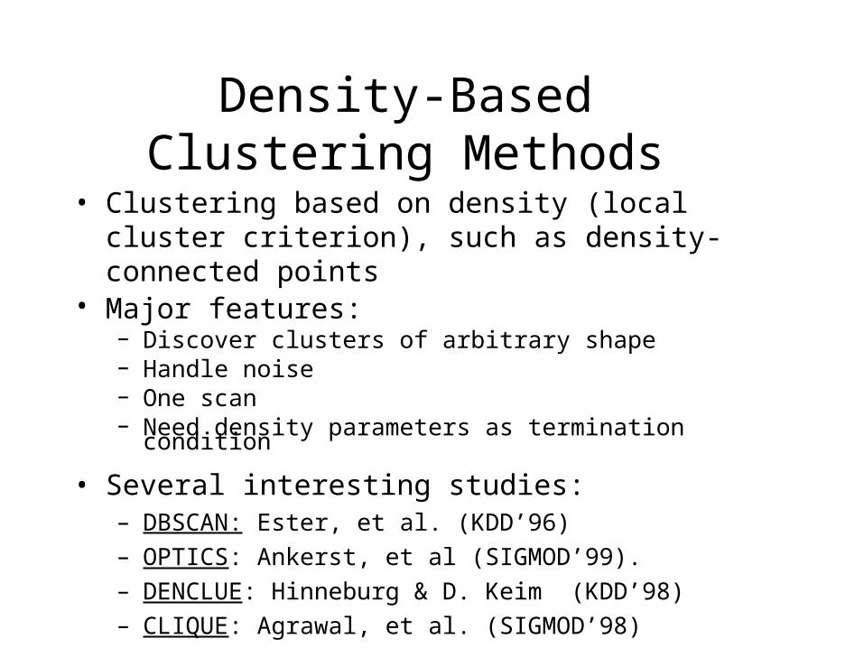
Density-Based Clustering Methods

• Clustering based on density (local cluster criterion), such as density-connected points

• Major features:– Discover clusters of arbitrary shape– Handle noise– One scan– Need density parameters as termination condition

• Several interesting studies:– DBSCAN: Ester, et al. (KDD’96)

– OPTICS: Ankerst, et al (SIGMOD’99).

– DENCLUE: Hinneburg & D. Keim (KDD’98)

– CLIQUE: Agrawal, et al. (SIGMOD’98)

Model based clustering

• Assume data generated from K probability distributions

• Typically Gaussian distribution Soft or probabilistic version of K-means clustering

• Need to find distribution parameters.

• EM Algorithm

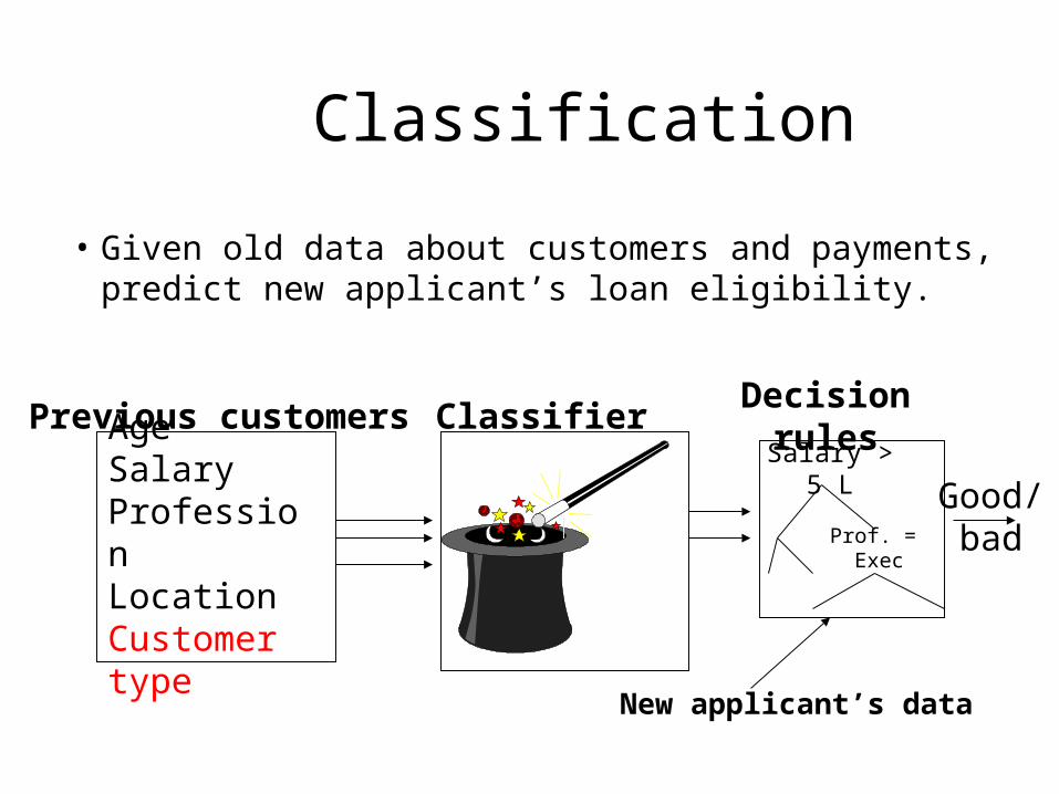
Classification

• Given old data about customers and payments, predict new applicant’s loan eligibility.

AgeSalaryProfessionLocationCustomer type

Previous customers Classifier Decision rules

Salary > 5 L

Prof. = Exec

New applicant’s data

Good/bad

• Tree where internal nodes are simple decision rules on one or more attributes and leaf nodes are predicted class labels.

Decision trees

Salary < 1 M

Prof = teaching

Good

Age < 30

BadBad Good

Building treeGrowTree(TrainingData D)

Partition(D);

Partition(Data D)if (all points in D belong to the same class) then

return;for each attribute A do

evaluate splits on attribute A;use best split found to partition D into D1 and D2;Partition(D1);Partition(D2);

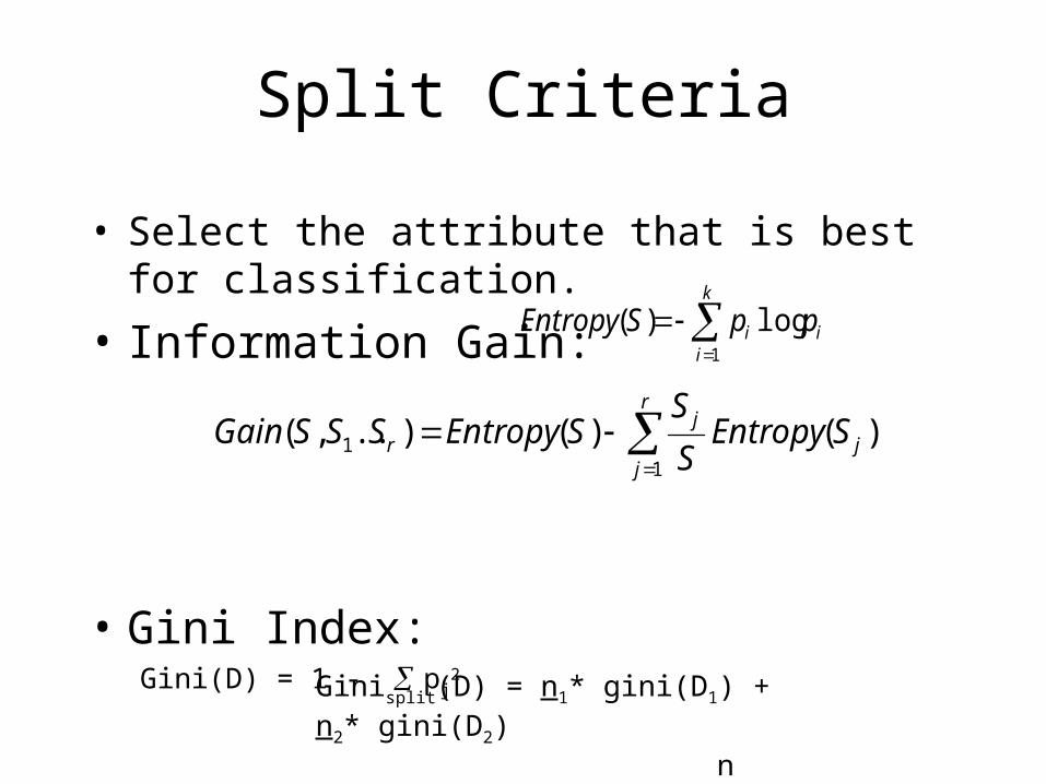
Split Criteria

• Select the attribute that is best for classification.

• Information Gain:

• Gini Index:Gini(D) = 1 - pj

2

k

iii ppSEntropy

1

log)(

r

jj

jr SEntropy

S

SSEntropySSSGain

11 )()()..,(

Ginisplit(D) = n1* gini(D1) + n2* gini(D2) n n

SLIQ (Supervised Learning In Quest)

• Decision-tree classifier for data mining

• Design goals:– Able to handle large disk-resident training sets– No restrictions on training-set size

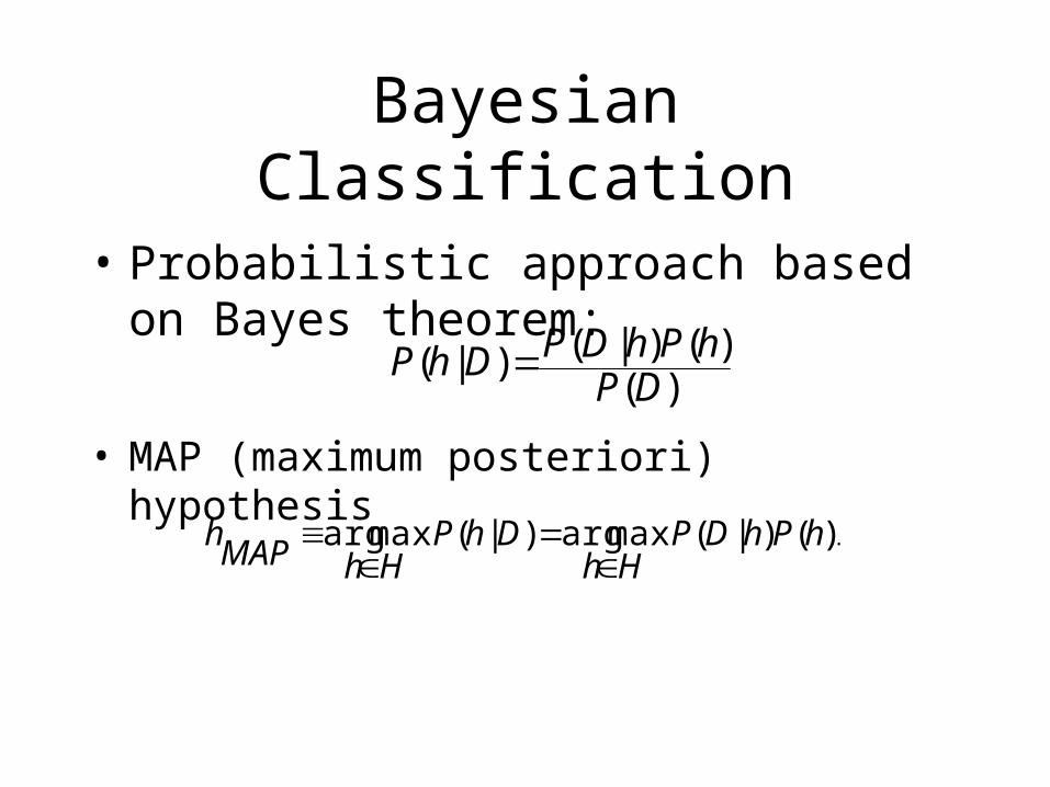
Bayesian Classification

• Probabilistic approach based on Bayes theorem:

• MAP (maximum posteriori) hypothesis

)()()|()|(

DPhPhDPDhP

.)()|(maxarg)|(maxarg hPhDPHh

DhPHhMAP

h

Bayesian Belief Networks (I)Age

Diabetes

Insulin

FamilyH

Mass

Glucose

M

~M

(FH, A) (FH, ~A)(~FH, A)(~FH, ~A)

0.8

0.2

0.5

0.5

0.7

0.3

0.1

0.9

Bayesian Belief Networks

The conditional probability table for the variable Mass