Reverse Top-k Search using Random Walk with Restart ∗

Adams Wei Yu†§, Nikos Mamoulis§, Hao Su‡†School of Computer Science, Carnegie Mellon University

§Department of Computer Science, The University of Hong Kong‡Computer Science Department, Stanford University

weiyu@cs.cmu.edu, nikos@cs.hku.hk, haosu@cs.stanford.edu

ABSTRACTWith the increasing popularity of social networks, large volumesof graph data are becoming available. Large graphs are also de-rived by structure extraction from relational, text, or scientific data(e.g., relational tuple networks, citation graphs, ontology networks,protein-protein interaction graphs). Node-to-node proximity is thekey building block for many graph-based applications that searchor analyze the data. Among various proximity measures, randomwalk with restart (RWR) is widely adopted because of its abilityto consider the global structure of the whole network. AlthoughRWR-based similarity search has been well studied before, there isno prior work on reverse top-k proximity search in graphs based onRWR. We discuss the applicability of this query and show that itsdirect evaluation using existing methods on RWR-based similaritysearch has very high computational and storage demands. To ad-dress this issue, we propose an indexing technique, paired with anon-line reverse top-k search algorithm. Our experiments show thatour technique is efficient and has manageable storage requirementseven when applied on very large graphs.

1. INTRODUCTIONGraph is a fundamental model for capturing the structure of data

in a wide range of applications. Examples of real-life graphs in-clude, social networks, the Web, transportation networks, citationgraphs, ontology networks, and protein-protein interaction graphs.In most applications, a key concept is the node-to-node proxim-ity, which captures the relevance between two nodes in a graph. Awidely adopted proximity measure, due to its ability to capture theglobal structure of the graph, is random walk with restart (RWR).RWR proximity from node u to node v, is the probability for arandom walk starting from u to reach v after infinite time; at anytransition there is a chance α (0 < α < 1) that the random walkrestarts at u. Compared to other measures (like shortest path dis-tance), a significant advantage of RWR is that it takes into accountall the possible paths between two nodes. Other merits of RWR isthat it can model the multi-faceted relationship between two nodes∗Supported by grant HKU 715413E from Hong Kong RGC. Workdone while the first author was with HKU.

This work is licensed under the Creative Commons Attribution-NonCommercial-NoDerivs 3.0 Unported License. To view a copy of this li-cense, visit http://creativecommons.org/licenses/by-nc-nd/3.0/. Obtain per-mission prior to any use beyond those covered by the license. Contactcopyright holder by emailing info@vldb.org. Articles from this volumewere invited to present their results at the 40th International Conference onVery Large Data Bases, September 1st - 5th 2014, Hangzhou, China.Proceedings of the VLDB Endowment, Vol. 7, No. 5Copyright 2014 VLDB Endowment 2150-8097/14/01.

[13] and that RWR is stable to small changes in the graph [20].RWR has been successfully applied in the search engine Google[21] to rank the importance of web pages. In addition, several othermeasures build upon RWR, including Personalized Pagerank [12],ObjectRank [5], Escape Probability [25], and PathSim [23].

Many search and analysis tasks rely on proximity computations.These include, citation analysis in bibliographical graphs [14], linkprediction in social networks [19], graph clustering [2], and makingrecommendations [16]. The top-k RWR proximity query retrievesthe k nodes with the highest proximity from a given query nodeq in a graph. This problem has been investigated previously andefficient solutions have been proposed for it (e.g., [11, 3, 10]).

In this paper, we study the reverse top-k RWR proximity query:given a node q, find all the nodes that have q in their top-k RWRproximity sets. Reverse top-k queries can be used for detection ofspam nodes in a graph. Search engines, such as Google, aggregatethe RWR proximities from all other nodes to one node in a singlevalue, known as PageRank. Thus, the proximity from web page uto v can be interpreted as the PageRank contribution that u makesto v. When a node q is suspected to be a spam web page, one couldrun a reverse top-k search on q, and find out the pages which giveone of their top-k contributions to q. If the answer set contains alarge proportion of web pages already labeled as spam, then q islikely to be a spam too. As another application, consider an authorin a co-authorship network who wishes to find the set of people thatregard himself as the one of their most important direct or indirectcollaborators. The reverse top-k result can be used for identifyingthe likelihood of successful collaborations in the future. The size ofan author’s reverse top-k list is also an indicator of his popularity inthe community. Finally, in a product co-purchase graph, a reversetop-k query of a product q can identify which products influencethe buying of q. One can leverage this information to promote q infuture transactions.

To the best of our knowledge, there is no previous work on re-verse top-k RWR-based search in large graphs. In addition, ex-tending solutions for top-k RWR search to compute reverse top-kqueries is not trivial. Specifically, while for a top-k search we onlyneed to find the top-k proximity set of a single node q, the reversetop-k search must compute the top-k sets of all nodes in the graphand check whether q appears in each of them. Therefore, a re-verse top-k query is substantially more expensive than top-k RWRsearch. Figure 1 illustrates a toy graph of 6 nodes and the entireproximity matrix P computed from it; the i-th column pi of Pcontains the proximity values from node i to all nodes in the graph(e.g., the proximity from node 1 to node 3 is 0.12). In each columnpi, the k = 2 largest entries are shaded; these indicate the results ofa top-2 query from node i (e.g., the top-2 query from node 3 returnsnodes 2 and 3). Observe that for any given node q, to answer a top-

401

1

5

6

4

2

3

The  node  1,  2  is  the  hubs�

0.32  0.28  0.12  0.13  0.06  0.09  

0.24  0.39  0.17  0.10  0.04  0.07  

0.24  0.29  0.27  0.10  0.04  0.07  

0.19  0.31  0.13  0.23  0.10  0.05  

0.20  0.33  0.14  0.08  0.18  0.06  

0.18  0.30  0.13  0.14  0.06  0.20  

p1 p2 p3 p4 p5 p6P

Figure 1: Example graph and its proximity matrix

2 query, we only have to compute and access the values of a singlecolumn, whereas a reverse top-2 query for a node i requires findingall the shaded entries in the i-th row (e.g., the reverse top-2 queryfor node 1 returns nodes 1, 2, and 5). To find whether an entry isshaded or not, we have to compute the entire matrixP and rank thevalues in each column. Computing the whole proximity matrix isboth time and space-consuming, especially for large graphs.

We propose a reverse top-k query evaluation framework whichalleviates this issue. In a nutshell, our approach computes (at a pre-processing step) from the graph G (having |V | nodes) a graph in-dex, which is based on aK×|V |matrix, containing in each columnv the K largest approximate proximity values from v to any othernodes in G. K is application-dependent and represents the highestvalue of k in a practical query. At each column v of the index, theapproximate values are lower bounds of the K largest proximityvalues from v to all other nodes, computed after adapting and par-tially executing Berkhin’s Bookmark Coloring Algorithm (BCA)[7]. Given the graph index and a reverse top-k query q (k ≤ K),we prove that the exact proximities from any node v to query q canbe efficiently computed by applying the power method. By com-paring these with the corresponding lower bounds taken from thek-th row of the graph index, we are able to determine which nodes(i.e., columns ofP ) are certainly not in the reverse top-k result of q.For some of the remaining nodes, we may also be able to determinethat they are certainly in the reverse top-k result, based on derivedupper bounds for the k-th largest proximity value from them. Fi-nally, for any candidate that remains, we progressively refine itsapproximate proximities, until based on its lower or upper boundwe can determine if it should be in the result. The proximities re-fined during query processing can be updated into the graph index,making its values progressively more accurate for future queries.

Our contributions can be summarized as follows:

• We study for the first time reverse top-k proximity queriesbased on RWR in large graphs.• We propose a dynamically refined, space-efficient index

structure, which supports reverse top-k query evaluation.The index is paired with an efficient online query algorithm,which prunes a large number of nodes that are definitely inor not in the reverse top-k result and minimizes the requiredrefinement for the remaining candidates.• A side contribution of our online algorithm is a proof that we

can apply the power method for computing the exact proxim-ities from all nodes to a given node q. This result can serveas a module of any applications that need to compute RWRproximities to a given node.• We conduct an experimental study demonstrating the effi-

ciency of our framework, as well as the effectiveness of thereverse top-k RWR query in real graph applications.

The remainder of this paper is organized as follows. Section 2provides a definition for the RWR-based proximity vector whichcaptures the proximities from a given node to all other nodes and

GeneralA Transition probability matrixP Proximity matrixpu Proximity vector from node u to other nodeseu Unit vector having eu(u) = 1, and eu(v) = 0 ∀v 6= u

pkmaxu The k-th largest entry of pu

BCA starting from node uptu (rtu) Retained (residue) ink distribution at iteration tstu (wt

u) Ink accumulated at hubs (non-hubs) at iteration tpu (ptu) Descending ranked list of pu(ptu)lbtu (ubtu) Lower (upper) bound of ptu(k)

Table 1: Main notations

reviews methods for computing it. The reverse top-k RWR prox-imity search problem is formalized in Section 3 and the baselinebrute force solution is discussed. In Section 4, we present our so-lution which is experimentally evaluated in Section 5. In Section6, we briefly discuss previous work related to reverse top-k RWRproximity search. Finally, Section 7 concludes the paper.

2. PRELIMINARIESIn this section, we first provide definitions for the RWR proxim-

ity matrix of a graph and the proximity vectors of nodes in it. Then,we review the Bookmark Coloring Algorithm (BCA) [7] for com-puting the RWR proximity from a given node to all other nodes,based on which our offline index is built. For a matrix M , mj orm∗,j denotes its j-th column, mi,∗ denotes its i-th row, and mi,j

denotes the element of its i-th row and j-th column. For a vectorv, v(i) denotes its i-th entry and v(1 : i) denotes its first i entries.Table 1 summarizes the main symbols used in the paper.

2.1 DefinitionsLetG = (V,E) be a directed graph, with a set V = {1, 2, ..., n}

of vertices and a set E ⊂ V × V of edges. Let n = |V |,m = |E|,A = [a1,a2, ...,an] ∈ Rn×n be the column-stochastic transitionprobability matrix, and OD(i) be the out-degree of node i. Weassume that ai,j = 1

OD(j)if edge j → i exists and ai,j = 0,

otherwise.1 In other words, the RWR transition probability fromnode j to any of its out-neighbors i only depends on the out-degreeof j (i.e., all out-neighbors are equally likely to be visited). For agiven node u, the RWR proximity values from it to other nodes isthe solution of the following linear system w.r.t. pu:

pu = (1− α)Apu + αeu, (1)

where pu ∈ Rn is the proximity vector of node u, with pu(v)denoting the proximity from u to v; eu ∈ Rn is a unit vector havingeu(u) = 1 and all other values set to 0, and α ∈ [0, 1] denotes therestart probability in RWR (typically, α = 0.15). The analyticalsolution is

pu = Peu, (2)

where P = α · (I − (1− α)A)−1 = [p1,p2, ...,pn] is called theproximity matrix. In fact, P can also be used to compute the Pager-ank (pr) and any Personalized Pagerank (ppr) vector as follows:

pr =1

nPe, pprv = Pv, (3)

1In the case where dangling nodes with no outgoing edges exist,we can simply delete them, or add a sink node which links to itselfand is pointed by each dangling node.

402

where e ∈ Rn has 1 in all entries and v ∈ Rn is any given per-sonalized vector such that ∀1 ≤ i ≤ n, vi ≥ 0 and ‖v‖1 =∑ni=1 |vi| = 1.Computing P at its entirety or partially is a key problem in dif-

ferent applications. Approaches like the iterative Power Method(PM) [21] and Monte Carlo Simulation (MCS) [9] can be used tocompute an approximate value for a single proximity vector puand/or the entire matrix P . PM converges to an accurate pu whileMCS is less accurate but faster. Next, we discuss in detail an effi-cient technique for deriving a lower-bound of pu.

2.2 Bookmark Coloring Algorithm (BCA)Basic model. Berkhin [7] models RWR by a bookmark coloring

process, which facilitates the efficient estimation of pu. We beginby injecting a unit amount of colored ink into u, with an α portionretained in u and the rest (1−α) portion evenly distributed to eachof u’s out-neighbors. Each node which receives ink retains an αportion of the ink and distributes the rest to its out-neighbors. Atan intermediate step t(= 0, 1, 2, ...), we can use two vectors ptu,rtu ∈ Rn to capture the ink distribution in the whole graph, whereptu(v) is the ink retained at node v, and rtu(v) is the residue ink tobe distributed from v. When rtu(v) reaches 0 for all v ∈ V (i.e.,‖ru‖1 = 0), ptu is exactly pu; the proximity vector pu can be seenas a stable distribution of ink. In fact, BCA can stop early, at a timet, where rtu(v) values are small at all nodes v; ptu is then a sparselower-bound approximation of pu [7].

Hub effects. In the process of ink propagation, some of thenodes may have a high probability to receive new ink and distributepart of it again and again. Such nodes are called hubs and their set isdenoted by H = {h1, h2, ..., h|H|}. Without loss of generality, weassume that the first |H| nodes in V are the hubs. If we knew howhubs distribute their ink across the graph (i.e., if we have precom-puted the exact proximity vector ph for each h ∈ H), we wouldnot need to distribute their residue ink during the process of com-puting pu for a node u ∈ V \ H . Instead, we could accumulateall the residue ink at hubs, and distribute it in batch at the end bya simple matrix multiplication. In [7], a greedy scheme is adoptedto select hubs and implement this idea. It starts by applying BCAon one node and selecting the node with the largest retained ink asa hub. This process is repeated from another starting node to selectanother hub, until a sufficient number of hubs are chosen. Oncethe hub nodes are selected, we can use the power method (PM) tocalculate the exact vector ph for each h ∈ H.

BCA using hubs. Assume that we have selected a set of hubsHand have pre-computed ph for each h ∈ H. To compute pu for anon-hub node u, BCA [7] (and its revised version [2]) first injectsa unit amount of ink to u, then u retains an α portion of the ink,and distributes the rest to u’s out-neighbors. At each propagationstep t, BCA picks a non-hub node vt and distributes the residueink rt−1

u (vt) to its out-neighbors. Two vectors stu and wtu ∈ Rn

are introduced and maintained in this process. stu is used to storethe ink accumulated at hubs so far and wt

u is used to store the inkretained at non-hub nodes. Thus, for a hub node h, stu(h) is the inkaccumulated at h by time t; this ink will be distributed to all nodesin batch after the final iteration, with the help of the (pre-computed)ph. For a non-hub node v, wt

u(v) stores the ink retained so far atv (which will never be distributed). wt

u(v) (stu(v)) is always zerofor a hub (non-hub) node v. The following equations show how allvectors are updated at each step:

wtu = αrt−1

u (vt) · evt +wt−1u (4)

rtu = (1− α)rt−1u (vt) · avt + [rt−1

u − rt−1u (vt) · evt ] (5)

stu =∑i∈H

rt−1u (i) · ei + st−1

u (6)

According to the first part of Eq. (4), an α ink portion ofrt−1u (vt) is retained at vt. Eq. (5) subtracts the residue inkrt−1u (vt) from vt (second part) and evenly distributes the remain-

ing (1− α) portion to vt’s out-neighbors (first part). Eq. (6) accu-mulates the ink that arrives at hub nodes. At any step t, BCA cancompute ptu and use it to approximate pu, as follows:

ptu = wtu + PH · stu (7)

where PH = [p1,p2, ...,p|H|,0n×(n−|H|)] ∈ Rn×n, i.e., PH isthe proximity matrix including only the (precomputed) proximityvectors of hub nodes and having 0’s in all proximity entries of non-hub nodes. ptu is computed only when all residue values are small;in this case, it is deemed that ptu is a good approximation of pu. Inorder to reach this stage, at each step, a vt with large residue inkshould be selected. In [7], vt is selected to be the node with thelargest residue ink, while in [2] vt is any node with more residueink than a propagation threshold η. BCA terminates when the to-tal residue ink does not exceed a convergence threshold ε or whenthere is no node with at least η residue ink.

3. PROBLEM FORMALIZATIONThe reverse top-k RWR query is formally defined as follows:

PROBLEM 1. Given a graph G(V,E), a query node q ∈ Vand a positive integer k, find all nodes u ∈ V , for which pkmaxu ≤pu(q), where pu is obtained by Eq. (1) and pkmaxu is the k-thlargest value in pu.

A brute-force (BF) method for evaluating the query is to (i) com-pute the proximity vector pu of every node u in the graph, and (ii)find all nodes u for which pkmaxu ≤ pu(q). BF requires the com-putation of the entire proximity matrix P . No matter which methodis used to compute the exact P (e.g., PM or the state-of-the-art K-dash algorithm [10]), examining the top-k values at each columnpu results in a O(n3) total time complexity for BF (or O(nm)for sparse graphs with n nodes and m edges), which is too high,especially for online queries on large-scale graphs.

There are several observations that guide us to the design of anefficient reverse top-k RWR algorithm. First, the expected num-ber of nodes in the answer set of a reverse top-k query is k; thusthere is potential of building an index, which can prune the major-ity of nodes definitely not in the answer set. Second, as noted in [4]and observed in our experiments, the power law distribution phe-nomenon applies on each proximity vector: typically, only few en-tries have significantly large and meaningful proximities, while theremaining values are tiny. Third, we observe that verifying whetherthe query node q lies in the top-k proximity set of a certain node uis a far easier problem than computing the exact top-k set of nodeu; we can efficiently derive upper and lower bounds for the prox-imities from u to all other nodes and use them for verification. Inthe next section, we introduce our approach, which achieves signif-icantly better performance than BF.

4. OUR APPROACHOur method focuses on two aspects: (i) avoiding the computa-

tions of unnecessary top-k proximity sets and (ii) terminating thecomputation of each top-k proximity set as early as possible. Theoverall framework contains two parts: an offline indexing module(Section 4.1) and an online querying algorithm (Section 4.2).

403

4.1 Offline IndexingFor our index design, we assume that the maximum k in any

query does not exceed a predefined value K, i.e. k ≤ K. For eachnode v, we compute proximity lower bounds to all other nodes andstore the K largest bounds to a compact data structure. The indexis relatively efficient to obtain, compared to computing the exactproximity matrix P . Given a query q and a k ≤ K, with the helpof the index, we can prune nodes that are guaranteed not to have q intheir top-k sets, thus avoiding a large number of unnecessary prox-imity vector computations. The index is stored in a compact format,so that it can fit in main memory even for large graphs. It also sup-ports dynamic updating after a query has been completed; this way,its performance potentially improves for any future queries.

The lower bounds used in our index are based on the fact that,while running BCA from any node u ∈ V , each entry of ptu atiteration t is monotonically increasing w.r.t. t; formally:

PROPOSITION 1. ∀u, v ∈ V , p1u(v) ≤ p2

u(v) ≤ ... ≤ pu(v).

PROOF. See [29].

Thus, after each iteration t of BCA from u ∈ V , we can have alower bound ptu(v) of the real proximity value pu(v) from u to anynode v ∈ V . The following proposition shows that the k-th largestvalue in ptu serves as a lower bound for the k-th largest proximityvalue in pu:

PROPOSITION 2. Let ptu(k) be the k-th largest value in ptu af-ter t iterations of BCA from u. Let pu(k) be the k-th largest valuein pu. Then, ptu(k) ≤ pu(k) = pkmaxu .

PROOF. See [29].

Note that this is a nice property of BCA, which is not presentin alternative proximity vector computation techniques (i.e., PMand MCS). Besides, we observe that by running BCA from a nodeu, the high proximity values stand out after only a few iterations.Thus, to construct the index, we run an adapted version of BCAfrom each node u ∈ V that stops after a few iterations t to derivea lower-bound proximity vector ptu. Only the K largest values ofthis vector are kept in descending order in a ptu(1 : K) vector.Our index consists of all these lower bounds; in Section 4.2, weexplain how it can be used for query evaluation. In the remain-der of this subsection, we provide details about our hub selectiontechnique (Section 4.1.1), our adaptation of BCA for deriving thelower-bound proximity vectors and constructing the index (Section4.1.2), and a compression technique that reduces the storage re-quirements of the index (Section 4.1.3).

4.1.1 Hub SelectionThe hub selection method in [7], runs BCA itself to find hubs;

its efficiency thus heavily relies on the graph size and the numberof selected hubs. We use a simpler approach, which is independentof these factors and hence can be used for large-scale graphs. Weclaim that nodes with high in-degree or out-degree are already goodcandidates to be suitable hubs. Therefore we define H as the unionof the sets of high in-degree nodes Hin and high out-degree nodesHout. Hin (Hout) is the set ofB nodes in V with the largest in-degree(out-degree). In Section 5, we investigate choices for parameter B.

4.1.2 BCA AdaptationWe propose an improved ink propagation strategy for BCA com-

pared to those suggested by [7] and [2]. Instead of propagatinga single node’s residue ink at each iteration t, our strategy se-lects a subset of nodes Lt, which includes those having no less

residue ink than a given propagation threshold η; i.e., Lt = {v ∈V \ H|rt−1

u (v) ≥ η}. η is selected such that only significantresidue ink is propagated. The rules for updating stu and ptu arethe same as shown in Eq. (6) and (7), respectively. However, theupdateswt

u and rtu are performed as follows:

wtu =

∑i∈Lt

αrt−1u (i) · ei +wt−1

u (8)

rtu =∑i∈Lt

(1− α)rt−1u (i) · ai + [rt−1

u −∑i∈Lt

rt−1u (i) · ei] (9)

To understand the advantage of our strategy, note that the maincost of BCA at each iteration consists of two parts. The first isthe time spent for selecting nodes to propagate ink from and thesecond is the time spent on updating vectors rtu, stu, andwt

u.2 Ourapproach reduces both costs. First, selecting a batch of nodes at atime significantly reduces the total remaining residue ‖rtu‖1 in asingle iteration and greatly reduces the overall number of iterationsand thus the total number of vector updates. Second, since at eachiteration both finding a single node or a set of nodes to propagateink from requires a linear scan of rt−1

u , the total node selectiontime is also reduced.

Our BCA adaptation ends as soon as the total remaining ink‖rtu‖1 is no greater than a residue threshold δ. We observe that‖rtu‖1 drops drastically in the first few iterations of BCA and thenslowly in the latter iterations. Thus, we select δ such that our BCAadaptation terminates only after a few iterations, deriving a roughapproximation of pu that is already sufficient to prune the majorityof nodes during search.

The complete lower bound indexing procedure is described byAlgorithm 1. Let tu be the number of iterations until the termina-tion of BCA from u and t = [t1, t2, ..., tn]. The index resultingfrom Algorithm 1 is denoted by It = (P t,Rt,W t,St,PH),where P t = [pt11 (1 : K), ..., ptnn (1 : K)] is the top-K lowerbound matrix storing the K largest values of each ptuu , Rt =[rt11 , ..., r

tnn ] is the residue ink matrix,W t = [wt1

1 , ...,wtnn ] is the

non-hub retained ink matrix, St = [st11 , ..., stnn ] is the hub accu-

mulated ink matrix and PH is the hub proximity matrix. Wheneverthe context is clear, we simply denote ptuu by ptu and the index byI = (P ,R,W ,S,PH).

Algorithm 1 Lower Bound Indexing (LBI)Input: Matrix A, number K, Hubs H , Residue threshold δ, Propaga-tion threshold η.Output: Index I = (P ,R,W ,S,PH ).

1: for all h ∈ H do2: Compute ph by power method or BCA;3: for all nodes u ∈ V do4: tu = 0; rtuu = eu; stuu = wtu

u = 0;5: while ‖rtuu ‖1 > δ do6: tu = tu + 1;7: Update rtuu , stuu , wtu

u by Eq. (9), (6), (8);8: Compute ptuu by Eq. (7);9: ptuu = top K entries of ptuu in descending order;

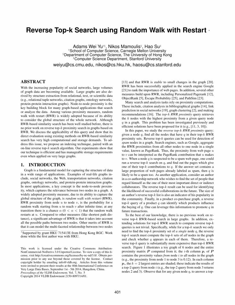
Figure 2 illustrates the result of our indexing approach on thetoy graph of Figure 1, for α = 0.15. First, by setting B = 1,we select the two nodes with the highest in- and out-degrees tobecome hubs. These are nodes 1 and 2. For these two nodes theexact proximity vectors p1 and p2 are computed and stored in the2Recall that ptu needs not be updated at each iteration and is onlycomputed at the end of BCA or when an approximation of pushould be obtained.

404

The  nodes  1,  2  are  the  hubs�

0.32  0.28  0.12  0.13  0.06  0.09  

0.24  0.39  0.17  0.10  0.04  0.07  

0.24  0.29  0.27  0.10  0.04  0.07  

0.10  0.17  0.07  0.19  0.08  0.03  

0.20  0.33  0.14  0.08  0.18  0.06  

0.10  0.17  0.07  0.10  0.02  0.18  

0.32  0.28  0.13  

0.39  0.24  0.17  

0.29  0.27  0.24  

0.19  0.17  0.10  

0.33  0.20  0.18  

0.18  0.17  0.10  

1

5

6

4

2

3

p1 p2 pt33 pt4

4 pt55 pt6

6

Pp1 p2 pt3

3 pt44 pt5

5 pt66

Figure 2: Example of top-3 lower bound index

hub proximity matrix PH = [p1,p2,0,0,0,0]. For the remainingnodes, we run our BCA adaptation with propagation threshold η =10−4 and residue threshold δ = 0.8, which results in the pt33 –pt66 vectors shown in the figure. Finally, we select from each of{p1,p2,p

t33 , . . . ,p

t66 } the top-K values (for K = 3) and create

the lower bound matrix P = [p1, p2, pt33 , p

t44 , p

t55 , p

t66 ], as shown

in the figure. Note that ‖rt33 ‖1 = ‖rt55 ‖1 = 0 and ‖rt44 ‖1 =‖rt66 ‖1 = 0.36.

4.1.3 Compact Storage of the IndexThe space complexity for the hub proximity matrix PH of I is

O(|H|n), where |H| (n) is the number of hub (total) nodes. Thematrix may not fit in memory if n and |H| are large. We apply acompression technique for PH , based on the observation that thevalues of a proximity vector follow a power law distribution; ineach vector ph ∈ PH , the great majority of values are tiny; onlya small percentage of these values are significantly large. There-fore, we perform rounding by zeroing all values lower than a givenrounding threshold ω. In our implementation, we choose an ω thatcan save much space without losing reverse top-k search precision.If sufficient hubs are selected, matrices R,W ,S are sparse, sothe storage cost for the index I will mainly be due to P and therounded PH . The following theorem gives an estimation for thetotal index storage requirements after the rounding operation.

THEOREM 1. ∀h ∈ H , given rounding threshold ω, if the val-ues of ph follow a power law distribution, i.e., the sorted valueph(i) ∝ i−β , where 0 < β < 1 is the exponent parameter,then the space required to store the whole index is O(Kn + (1 −β)

1β |H|ω−

1β n

1− 1β ).

PROOF. Let ph(i) = γi−β . As

1 =

n∑i=1

ph(i) = γ

n∑i=1

i−β ≈ γnβ−1

∫ 1

0

x−βdx =γnβ−1

1− β

we have γ ≈ (1 − β)nβ−1 and ph(i) ≈ (1 − β)nβ−1i−β . Letph(l∗) ≥ ω, then we have

l∗ ≤ (1− β)1β ω− 1β n

1− 1β

Since only less than l∗ entries need to be stored for a single hubnode, we need (1−β)

1β |H|ω−

1β n

1− 1β space forPH . Plus the top-

K lower bound space requirement O(Kn), the total index storagewould be O(Kn+ (1− β)

1β |H|ω−

1β n

1− 1β ).

Let ptuu

be the approximated proximities constructed by Eq. (7)with rounded hub proximities PH . We can trivially show that

Propositions 1 and 2 hold for ptuu

. Thus, ptuu

is still an increas-ing lower bound of pu and ptu

ucan replace the ptuu in our index. In

the following, we give a bound for the error caused by rounding.

PROPOSITION 3. Given rounding threshold ω and ph(i) ≈γi−β , where γ = (1− β)nβ−1, then for ∀u ∈ V ,

‖ptuu − ptuu ‖1 ≤ 1− (1− βωn

)1β−1.

PROOF. See [29].

We empirically observed (see Section 5) that our rounding ap-proach can save huge amounts of space and the real storage re-quirements are even much smaller than the theoretical bound givenby Theorem 1. Meanwhile, the actual error is much smaller thanthe theoretical bound by Proposition 3, and more importantly, it hasminimal effect to the reverse top-k results. To keep the index nota-tion uncluttered, we use PH to also denote the rounded hub prox-imities (i.e., PH ) and ptuu to denote the corresponding roundedproximity vectors ptu

ucomputed using PH .

4.2 Online Query AlgorithmThis section introduces our online reverse top-k search tech-

nique. Given a query node q ∈ V , we perform search in two steps.First, we compute the exact proximity from each u ∈ V to q us-ing a novel and efficient method (Section 4.2.1). In the second step(Section 4.2.2), for each node u we use the index described in Sec-tion 4.1 to prune u or add u to the search result, by deriving a lowerand an upper bound (denoted as lbtu and ubtu) of u’s k-th largestproximity value pkmaxu to other nodes and comparing it with itsproximity to q. For nodes u that cannot be pruned or confirmed asresults, we refine lbtu and ubtu using our index incrementally, until uis pruned or becomes a confirmed result. The refinement is used toupdate the index for faster future query processing (Section 4.2.3).In this section, we use pu and p∗,u interchangeably to denote theu-th column of the proximity matrixP ; also note that lbtu = ptu(k)and ubtu is the upper bound of pu(k) (= pkmaxu ) w.r.t. to ptu.

4.2.1 RWR Proximity to the Query NodeThe first step of our method is to compute the exact proximities

from all other nodes to the query q. Although a lot of previouswork has focused on computing the proximities from a given nodeu to all other nodes (i.e., a column p∗,u of the proximity matrixP ),there have only been a few efforts on how to find the proximitiesfrom all nodes to a node q (i.e., a row pq,∗ of P ). The authors ofthe SpamRank algorithm [6] suggest computing approximate prox-imity vectors p∗,u for all u ∈ V , and taking all pq,u to form pq,∗.However, to get an exact result, which is our target, such a methodwould require the computation of the entire P to a very high preci-sion, which leads to unacceptably high cost. A heuristic algorithmis proposed in [8], which first selects the nodes with high proba-bility to be the large proximity contributors to the query node, andthen computes their proximity vectors. This method requires thecomputation of several proximity vectors p∗,u to find only a subsetof entries in pq,∗. [1] introduces a local search algorithm that ex-amines only a small fraction of nodes, deriving, however, only anapproximation of pq,∗.

Although it seems inevitable to compute the whole matrix Pto get the exact proximities from all nodes to q, we show that thisproblem can be solved by the power method and has the same com-plexity as calculating a single column of P . Our result is novel andconstitutes an important contribution not only for the reverse top-ksearch problem that we study in this paper, but also for any problemthat includes finding the proximities from all nodes to a given node.

405

For example, our method could be used as a module in SpamRank[6] to find PageRank contributions that all nodes make to a givenweb page q precisely and efficiently.

First of all, we note that pq,∗ is essentially the q-th row of P ,hence, pq,∗ = eTq P = αeTq · (I − (1− α)A)−1, or equivalently

pTq,∗ = (1− α)ATpTq,∗ + αeq

(see Section 2 for the definitions of A, eq , and e). An interestingobservation is that p∗,u and pq,∗ are actually the solutions of thefollowing linear systems respectively,

xu = (1− α)Axu + αeu (10)

xq = (1− α)ATxq + αeq (11)

which share the same structure except, that eitherA orAT is usedas the coefficient matrix. This similarity motivates us to apply thepower method. Just as Eq. (10) can be solved by the iterative powermethod on matrix [(1− α)A+ αeue

T ]:

xi+1u = (1− α)Axiu + αeu = [(1− α)A+ αeue

T ]xiu, (12)

we hope that the linear system (11) could be solved by the follow-ing iterative method:

xi+1q = (1− α)ATxiq + αeq. (13)

However, showing that the sequence generated by Eq. (13) cansuccessfully converge to the solution of Eq. (11) is not trivial, asthe proof of the convergence of Eq. (12) does not apply for Eq.(13). The main difference between the two is as follows. In Eq.(12), if ‖x0

u‖1 = 1, then ‖xiu‖1 = eTxiu = 1 for i = 1, 2, ....Hence we can have the r.h.s. of Eq. (12) to prove {xiu}i to bea power method’s series and thus converges. Conversely, the se-quence {xiq}i is not non-expansive in the general case and we mayhave ‖xi+1

q ‖1 > ‖xiq‖1. In other words, we cannot transform Eq.(13) to the form of the r.h.s. of Eq. (12) to prove {xiq}i to be apower method’s series, so there is no obvious guarantee that it willconverge. We therefore have to prove that Eq. (13) converges to aunique vector, which is the solution of Eq. (11). Fortunately, us-ing techniques very different from the original convergence proofof Eq. (12), we show that Eq. (13) indeed converges to a uniquesolution, from an arbitrary initialization.

Let us lift xq ∈ Rn to space Rn+1 by introducing zq =

[xq1

].

The affine Equation (11) is now equivalent to

zq = Dqzq (14)

where Dq =

[(1− α)AT αeq

01×n 1

]∈ R(n+1)×(n+1). Then the

first n columns of (14) is exactly (11). Note that zq is an eigen-vector ofDq corresponding to eigenvalue 1. We will prove that zqis in fact the dominant eigenvector, therefore System (14) can besolved by the power method.

THEOREM 2. Let λ1 and λ2 be the first two largest eigenvaluesof Dq . Let z0

q = [(x0q)T , 1]T ,z∗q = [pq,∗, 1]T ∈ R(n+1), where

x0q is any vector in Rn, and let

zi+1q = Dqz

iq = Di+1

q z0q (15)

then the following conclusions hold:

(a) λ1 = 1 with multiplicity 1, and limi→∞ ziq = z∗q ,

limi→∞ xiq = pq,∗.

(b) λ2 = 1−α; the convergence rate of (15) and (13) is 1−α;

(c) For convergence tolerance ε, if i > log εα/ log(1− α), then

‖zi+1q − ziq‖1 ≡ ‖xi+1

q − xiq‖1 < ε.

PROOF. (a) Note that the row sum of Dq cannot exceed 1. Infact, for α > 0, it is obvious that the q-th row and the last rowhave row sum 1 and all other rows have row sum 1−α < 1. So thespectral radius ρ(Dq) ≤ maxi

∑j(Dq)ij ≤ 1. On the other hand,

z∗q 6= 0 satisfies Eq. (14), which implies that z∗q is the eigenvectorofDq with eigenvalue 1. Thus, λ1 = ρ(Dq) = 1.

Note that any eigenvector of value 1 must be a fixed point of Eq.(14). Therefore, if we can show that the sequence {ziq}i convergesto a nonzero point, it must be the unique eigenvector, and then themultiplicity of λ1 is 1. In the following, we will prove that thisstatement is true. It is easy to verify that

Diq =

[(1− α)i(AT )i α

∑i−1j=0(1− α)j(AT )jeq

01×n 1

]Since ‖AT ‖ = ρ(AT ) = 1, it follows that

‖(1− α)i(AT )i‖ ≤ (1− α)i‖AT ‖i ≤ (1− α)i, so

limi→∞

Diq =

[0n×n α[I − (1− α)AT )]−1eq01×n 1

]=

[0 P Teq0 1

],

implying that

limi→∞

ziq = limi→∞

Diqz

0q =

[0 P Teq0 1

] [x0q

1

]=

[pTq,∗

1

],

where pTq,∗ = P Teq . Hence limi→∞ ziq = z∗q and limi→∞ x

iq =

pq,∗. This also certifies that there is a unique convergence point of(15), so the multiplicity of λ1 is 1.

(b) RewriteDq = (1−α)

[AT 0n×1

01×n 1

]+αFq , where Fq =[

0n×n eq0n×1 1

]. Let ξ =

[01×n

1

]. It is easy to verify thatDT

q ξ = ξ.

As ρ(DTq ) = ρ(Dq) = 1, ξ is the eigenvector corresponding to the

largest eigenvalue of DTq and it is unique, since Dq and DT

q hasthe same eigenvalue multiplicity. Now we leverage the followinglemma to assist the rest of proof.

LEMMA 1. (From page 4 of [27]) If ξi is an eigenvector of Acorresponding to the eigenvalue λi, ζj is an eigenvector of AT

corresponding to λj and λi 6= λj , then ξTi ζj = 0.

By Lemma 1, the second largest eigenvector ζ of Dq must beorthogonal to ξ, i.e., ζT ξ = 0. By the structure of ξ, it must

be true that ζ =

[µ0

], µ is some vector in Rn, which implies

Fqζ = 0. Hence,Dqζ = (1−α)

[AT 00 1

]ζ = (1−α)

[ATµ

0

].

As Dqζ = λ2ζ, we have ATµ = λ21−αµ, indicating that µ is an

eigenvector ofAT . SinceA is a transition matrix, λ21−α ≤ ρ(A) =

1, so λ2 ≤ 1 − α. It is easy to verify that for ζ =

[en×1

0

],

Dqζ = (1 − α)ζ, so λ2 = 1 − α. In addition, the convergencerate of (15) is dictated by |λ2|/|λ1| = 1− α.

(c) Since {ziq}i is the power method’s series of Dq , we have‖zi+1q − ziq‖1 ≈ ‖( |λ2|

|λ1|)i(1 − |λ2|

|λ1|)‖ = (1 − α)iα. Hence, i >

log εα/ log(1− α) can lead to ‖zi+1

q − ziq‖1 < ε.

Theorem 2 shows that sequence {xiq}i, computed by Eq. (13) in-deed converges and also gives the estimated number of iterations.

406

Since it is part of the power method series {ziq}i, we can call Eq.(13) a power method; Algorithm 2 illustrates how to use it in solv-ing System (11) and deriving pq,∗. Note that the algorithm ter-minates as soon as the series converges based on the convergencethreshold ε (line 6).As it takes O(m) operations in each iteration(where m = |E| is the number of edges), the time complexity of

the algorithm is O(

log εα

log(1−α) ·m)

.

Algorithm 2 Power Method for Proximity to Node (PMPN)Input: Matrix A, Query q, Convergence tolerance ε.Output: Proximities pq,∗ from all nodes to q.

1: Initialize x0q as any vector ∈ Rn;

2: i = 0;3: repeat4: xi+1

q = (1− α)ATxiq + αeq ;5: i = i+ 1;6: until ‖xiq − xi−1

q ‖ < ε . convergence of PMPN7: pq,∗ = (xiq)

T ;

4.2.2 Upper Bound for the k-largest ProximityAfter having computed pq,∗, we know for each u ∈ V , the exact

proximity pu(q)(= pq,u) from u to q. Now, we access the k-throw of the lower bound matrix P of the index (see Section 4.1) andprune all nodes u for which lbtu = ptu(k) > pu(q). Obviously,if the k-th largest lower bound from u to any other node exceedspu(q), then it is not possible for q to be in the set of k closestnodes to u. For each node u that is not pruned, we compute anupper bound ubtu for the k-th largest proximity from u to any othernode, using the information that we have about u in the index. Ifpu(q) ≥ ubtu, then u is definitely in the answer set of the reversetop-k query. Otherwise, node u needs further processing.

We now show how to compute ubtu for a node u. Note that fromthe index, we have the descending top-K lower bound list ptu andthe residue ink vector rtu. For j = 1, 2, ..., k − 1, let

∆tj = ptu(j)− ptu(j + 1) (16)

zt0 = 0, and ztj = ztj−1 + j ·∆tk−j , 1 ≤ j ≤ k − 1 (17)

Then,

ubtu =

ptu(k − j)− ztj−‖r

tu‖1

j, if ∃ j ∈ [1, k − 1],

s.t. ztj−1 < ‖rtu‖1 ≤ ztjptu(1) +

‖rtu‖1−ztk−1

k, if ‖rtu‖1 > ztk−1

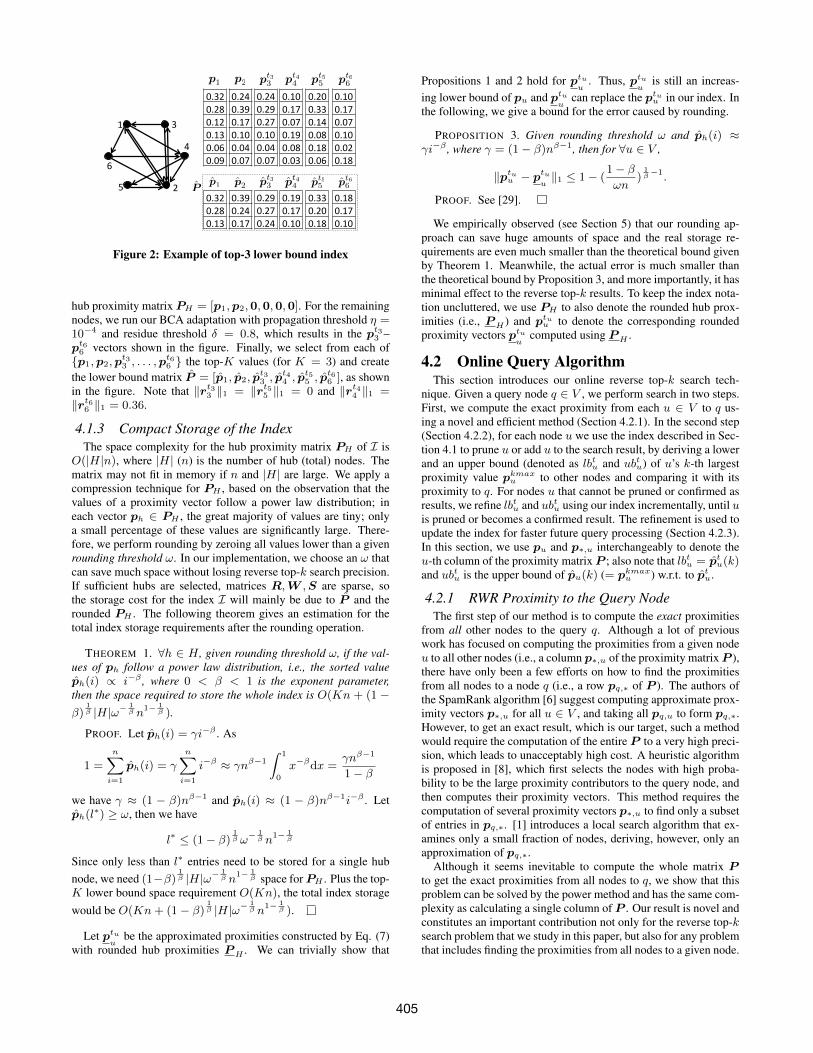
(18)Figures 3 and 4 illustrate the intuition and the derivation of ubtu.

Assume that k = 5 and the first k values of ptu are as shown on theleft of the figures, while the total remaining ink ‖rtu‖1 is shown onthe right of the figures. The best possible case for the k-th valueof pu is when ‖rtu‖1 is distributed such that (i) only the first kvalues may receive some ink, while all others receive zero ink and(ii) the ink is distributed in a way that maximizes the updated k-th value. To achieve (ii), ptu could be viewed as a staircase the khighest steps of which are fit tightly in a container. If we pour thetotal residue ink ‖rtu‖1 into the container, the level of the ink willcorrespond to the value of ubtu. ∆t

j is the difference between j-thand (j + 1)-th step of the staircase, while ztj is the ink required topour in order for its level in the container to reach the (k − j)-thstep. The first line of Eq. (18) corresponds to the case illustratedby Figure 3, where ubtu is smaller than pu(1), while the exampleof Figure 4 corresponds to the case of the second line, where thewhole staircase is covered by residue ink (‖rtu‖1 > ztk−1).

¢t1¢t1

¢t2¢t2

¢t3¢t3

¢t4¢t4

ptu(1)ptu(1)

ubtuubtu

krtuk1krtuk1

zt1zt1

zt2zt2

zt3zt3

ptu(2)ptu(2) pt

u(3)ptu(3) pt

u(4)ptu(4) pt

u(5)ptu(5) pt

u(6)ptu(6) pt

u(7)ptu(7)

Figure 3: Upper bound, k = 5, zt2 < ‖rtu‖1 ≤ zt3

ptu(7)ptu(7)pt

u(6)ptu(6)pt

u(5)ptu(5)pt

u(4)ptu(4)pt

u(3)ptu(3)pt

u(2)ptu(2)pt

u(1)ptu(1)

¢t1¢t1

¢t2¢t2

¢t3¢t3

¢t4¢t4

ubtuubtu

krtuk1krtuk1

zt4zt4

Figure 4: Upper bound, k = 5, ‖rtu‖1 > zt4

The following proposition states that ubtu is indeed an upperbound of the real k-largest value pkmaxu and is monotonically de-creasing as ptu(ptu) is refined by later iterations.

PROPOSITION 4. ∀u ∈ V , ub1u ≥ ub2u ≥ ... ≥ pkmaxu .

PROOF. See [29].

Algorithm 3 is a procedure for deriving the upper bound ubtu,given pu, ‖rtu‖1, and k. The algorithm simulates pouring ‖rtu‖1into the container by gradually computing the ztj values for j =1, 2, . . . , k− 1, until ztj−1 < ‖rtu‖1 ≤ ztj , which indicates that theresidue ink ‖rtu‖1 can level up to ptu(k− j). If ‖rtu‖1 > ztk−1, thewhole staircase is covered and the algorithm computes ubtu by thesecond line of Eq. (18). The complexity of Algorithm 3 is O(k),which is quite low compared to other modules.

Algorithm 3 Upper Bound Computation (UBC)Input: Matrix A, Number k, Node u, Lower bound vector ptu, Residueink vector rtu.Output: Upper bound ubtu of the k-th largest proximity from u.

1: zt0 = 0;2: for j = 1 to k − 1 do3: Compute ∆t

k−j by Eq. (16);4: Compute ztj by Eq. (17);5: if ztj−1 < ‖rtu‖1 ≤ ztj then6: Compute ubtu by first line of Eq. (18);7: return ubtu;8: Compute and return ubtu by second line of Eq. (18);

4.2.3 Candidate Refinement and Index UpdateWhen ptu(k) ≤ pq,u < ubtu, we cannot be sure whether u is a

reverse top-k result or not and we need to further refine the bounds

407

ptu(k) and ubtu. First, we apply one step of BCA in continuingthe computation of ptu and update ptu (lines 6-7 of Algorithm 1).Then, we apply Algorithm 3 to compute a new ubtu. This step-wiserefinement process is repeated while ptu(k) ≤ pq,u < ubtu; it stopsonce (i) pq,u < ptu(k), which means that q is not contained in thetop-k list of u, or (ii) pq,u ≥ ubtu, which means that u definitelyhas q as one of its top-k nearest nodes. In our empirical study, weobserved that for most of the candidates u, the process terminatesmuch earlier before the lower and upper bounds approach the exactvalue pq,u. Thus, many computations are saved.

If, due to a reverse top-k search, ptu(ptu) has been updated, wedynamically update the index to include this change. In addition,we update the corresponding stored values for rtu, stu, and wt

u.Due to this update, future queries will use tighter lower and upperbounds for u.

The complete online query (OQ) method is summarized by Al-gorithm 4. After computing the exact proximities to q (line 1), thealgorithm examines all u ∈ V and while a node u is a candidatebased on the lower bound ptuu (k) (line 4), we first check (line 5)whether the lower bound is the actual proximity (this happens when‖rtuu ‖1 = 0); in this case, u is added to the result set C and theloop breaks. Otherwise, the upper bound ubtuu is computed (line 8)to verify whether u can be confirmed to be a result; if u is not aresult (line 13), lines 6-7 of Algorithm 1 are run to refine ptuu (k);after the update, the lower bound condition is re-checked to seewhether u can be pruned or another loop is necessary. Note thatthe update besides increasing the values of ptuu (k) (i.e., increasingthe chances for pruning), it also reduces ubtuu , therefore the revisedupper bound ubtuu may render u a query result.

Algorithm 4 Online Query (OQ)Input: Matrix A, Query q, Number k, Index I.Output: Reverse top-k Set C of q, Updated Index I.

1: Compute the exact proximities pq,∗ by Algorithm 2;2: Initialize C = ∅;3: for all u ∈ V do4: while pu,q ≥ ptuu (k) do5: if ‖rtuu ‖1 = 0 then6: C = C ∪ u; . ptuu (k) = pu(k), so u is a result7: break;8: Compute ubtuu by Algorithm 3;9: if pu,q ≥ ubtuu then

10: C = C ∪ u; . u becomes a result11: break;12: else13: Update ptuu (k) by Algorithm 1;14: Save the updated P ,R,W ,S to I;

We now illustrate OQ with our running example. Consider thegraph and the constructed index shown in Figure 2. Assume thatq = 1 (i.e., the query node is node 1 in the graph) and k = 2.The first step is to compute pq,∗ using Algorithm 2; the resultis pq,∗ = [0.32, 0.24, 0.24, 0.19, 0.20, 0.18]. Now OQ loopsthrough all nodes u and checks whether pu,q ≥ ptuu (k). For thefirst node u = 1, we have 0.32 > 0.28 and ptuu (k) is the actualproximity pu(k) (recall that node 1 is a hub in our example, whoseproximities to other nodes have been computed), thus 1 is a result.The same holds for u = 2 (0.24 ≥ 0.24 and node 2 is a hub). Foru = 3, observe that pu,q < ptuu (k) (i.e., 0.24 < 0.27); thereforenode 3 is safely pruned (i.e., OQ does not enter the while loop foru = 3). Node u = 4 satisfies pu,q ≥ ptuu (k) (0.19 > 0.17) and‖rtuu ‖1 > 0, therefore the upper bound ubtuu = 0.36 is computedby Algorithm 3, however, pu,q < ubtuu , therefore we are still uncer-tain whether node 4 is a reverse top-k result. A loop of Algorithm

1 is run to update ptuu (k) to 0.23 (line 13); now node 4 is prunedbecause pu,q < ptuu (k) (0.19 < 0.23). Continuing the example,node 5 is immediately added to the result since p5,q = pt55 (k) and‖rt55 ‖1 = 0, whereas node 6 is pruned after the refinement of pt66 .

The following theorem shows the time complexity of OQ.

THEOREM 3. The time complexity of OQ in worst case is

O

((log ε

α+ |Cand| · log η

δ

log(1− α)

)·m)

where the ε is the convergence threshold of Algorithm 2, δ is theresidue threshold and η is the propagation threshold of Algorithm1, Cand is the set of candidates that could not be pruned immedi-ately by the index and m = |E| is the number of graph edges.

PROOF. The cost of a query includes the cost of Algorithm 2,which is O

(log ε

αlog(1−α) ·m

), as discussed in Section 4.2.1, and the

cost of examining and refining the candidates (lines 2 to 14 of OQ).The worst case is that all nodes in Cand cannot be pruned or con-firmed as result until we compute their exact k-th largest proximityvalues by repeating line 7 of Algorithm 1, i.e., until the maximumresidue ink maxi{rtuu (i)} at any node drops below η. Within aniteration, the update of one node u requires at most O(m) opera-tions Besides, each iteration is expected to shrink maxi{rtuu (i)}by a factor around (1 − α). Recall that since maxi{rtuu (i)} ≤ δ,the total number of iterations τ required to terminate BCA by mak-ing it smaller than η satisfies maxi{rtuu (i)} · (1 − α)τ ≈ η, i.e.,

τ ≈log η

maxi{rtuu (i)}

log (1−α) ≤ log ηδ

log(1−α) . Therefore, the total time com-

plexity in the worst case is O((

log εα+|Cand|·log η

δlog(1−α)

)·m)

.

As we show in Section 5.3, in practice, |Cand| is extremelysmall compared to n and most of the candidates can be pruned orconfirmed within significantly fewer than τ iterations. Hence, theempirical performance of OQ is far better than the worst case.

5. EXPERIMENTAL EVALUATIONThis section experimentally evaluates our approach , which is

implemented in Matlab 2012b. Our testbed is a cluster of 500 AMDOpteron cores (800MHz per core) with a total of 1TB RAM. Sinceour indexing algorithm can be fully parallelized (i.e., the approxi-mate proximity vectors of nodes are computed independently), weevenly distributed the workload to 100 cores to implement the in-dexing task. Each online query was executed at a single core andthe memory used at runtime corresponds to the size of our index(i.e., at most a few GBs as reported in Table 2). Hence, our solu-tion can also run on a commodity machine.

5.1 DatasetsWe conducted our efficiency experiments on a set of unlabeled

graphs. The number n = |V | (m = |E|) of nodes (edges) of eachgraph are shown in Table 2. Web-stanford-cs3 and Web-stanford4

were crawled from stanford.edu. Each node is a web domain and adirected link stands for a hyperlink between two nodes. Epinions4

is a ‘who-trust-whom’ social network from a consumer review siteepinions.com; each node is a member of this site, and a directededge i → j means that member i trusts j. Web-google4 a webgraph collected by Google. Experiments on two additional datasetsare included in [29].

3law.di.unimi.it/datasets.php4snap.stanford.edu/data/

408

5.2 Index ConstructionWe first evaluate the cost for constructing our index (Section 4.1)

and its storage requirements for different graphs and sizes |H| ofhub sets. After tuning, we set the index construction parameters(see Section 4.1) as follows: propagation threshold η = 10−4,residue threshold δ = 0.1, hub vector rounding threshold ω =10−6 for the first three graphs, and ω = 5 · 10−6 for the largestone. In all cases, K=200, the convergence threshold ε = 10−10

and the restart parameter α = 0.15. For a study on the effect ofthe different parameters and the rationale of choosing their defaultvalues, see [29].

Table 2 shows the index construction time for different graphs,for various values of the hub selection parameterB, which result indifferent sizes |H| of hub sets. The last column shows the time tocompute the entire proximity matrix P and its size on disk, whichrepresents the brute-force (BF) approach of just pre-computing andusing P for reverse top-k queries. The value in parentheses in thelast column is the minimum possible cost for our index, derived byjust storing the top-K lower bound matrix P and disregarding thestorage of the hub proximitiesPH and matricesR,W , andS. Thelast three rows for each graph show the space that our index wouldhave if we had not applied the compression technique discussed inSection 4.1.3, the actual space of our index, and the predicted spaceaccording to our analysis in Section 4.1.3 (i.e., using Theorem 1with β = 0.76, as indicated by [4]). The reported times sum up therunning time at each core, assuming the worst case of having justone single-core machine. Note that the actual time is roughly thereported time divided by the number of cores (100).

We observe that the best number of hubs to select in terms ofboth index construction cost and index size on disk depends onthe graph sparsity. For Web-stanford-cs, which is sparse graph, itsuffices to select less than 1% of the nodes with the highest in-and out- degrees as hubs, while for the denser Epinions and Web-stanford graphs 1% − 2% of the nodes should be selected. Theindex construction is much faster than the entire P computation,especially for larger and sparser graphs (e.g., for Web-google ittakes as little as 1.8% of the time to construct P ). The time is notaffected too much by the number of selected hubs.

The same observation also holds for the size of our index, whichis much smaller than the entire P and a few times larger than thebaseline storage of the top-K lower bound matrix P . Although ourindex also stores the hub matrix PH and matrices R, W , and S,its space is reasonable; the index can easily be accommodated inthe main memory of modern commodity hardware. The predictedspace according to our analysis is in most cases an overestimation,due to an under-estimation of the power law effect on the sparsityof proximity matrices. Note that our rounding approach generallyachieves significant space savings especially on large graphs (e.g.,Web-google). For each dataset, the index that we are using in sub-sequent experiments is marked in bold.

5.3 Online Query PerformanceWe now evaluate the performance of our index and our on-line

reverse top-k algorithm. We run a sequence of 500 queries on theindexes created in Section 5.2 and report average statistics for them.

Query Efficiency. Figure 5 shows the average runtime cost ofreverse top-k queries on different graphs, for different values ofk and with different options for using the index. Series “update”denotes that after each query is evaluated, the index is updated to“save” the changes in the P , R, W , and S matrices, while “no-update” means that the original index is used for each of the 500queries. We separated these cases in order to evaluate whether ourindex update policy brings benefits to subsequent queries which

Web-stanford-cs (|V | = 9914, |E| = 36854)B 50 100 200 300|H| 82 175 355 530

time (s) 31.5 31.6 34.2 40.4 365.5no rounding (MB) 55.2 57.4 65.3 77.9actual space (MB) 39.6 41.8 49.7 62.4 786 (15.8)pred. space (MB) 44.7 93.5 188 280

Epinions (|V | = 75879, |E| = 508837)B 1000 1500 2000 3000|H| 1484 2101 2690 3853

time (s) 15827 12285 11565 10792 139860no rounding (MB) 2778 2309 2284 2721actual space (MB) 2310 1696 1538 1716 46071 (121)pred. space (MB) 4220 5924 7551 10763

Web-stanford (|V | = 281903, |E| = 2312497)B 1000 1500 2000 3000|H| 1932 2866 3804 5586

time (s) 85503 89196 97462 111200 3263500no rounding (MB) 6506 8237 10209 14069actual space (MB) 1907 1639 1595 1638 635754 (451)pred. space (MB) 3977 5681 7393 10645

Web-google (|V | = 875713, |E| = 5105039)B 5000 10000 20000 50000|H| 9598 18871 37148 86246

time (s) 1024200 1107400 2206300 2865300 60162000no rounding (MB) 73362 137113 264315 607615actual space (MB) 5387 4727 4888 6897 6718720 (1466)pred. space (MB) 2874 4298 7103 14639

Table 2: Index construction time and space cost

apply on a more refined index. The case of “update” also bearsthe cost of updating the corresponding matrices. In either case,query evaluation is very fast compared to the brute-force approachof computing the entire P (the time needed for this is already re-ported in the last column of Table 2) for each graph. The updatepolicy results in significant reduction of the average query time insmall and dense graphs; however, for larger and sparser graphs theindex update has marginal effect in the query time improvementbecause there is a higher chance that subsequent queries are lessdependent on the index refinement done by previous ones. Notethat the workload includes 500 queries, which is a small numbercompared to the size of the graphs; we expect that for larger work-loads the difference will be amplified on large graphs.

Pruning Power of Bounds. Figure 6 shows, for the samequeries and the “update” case only, the average number (per query)of the candidates that are not immediately filtered using the lowerbounds of the index and also the number of nodes from these candi-dates that are immediately identified as hits (i.e., results) after theirupper bound computation. This means that only (candidates−hits)nodes (i.e., columns of P ) need to be refined on average for eachquery. We also show the average number of actual results for eachexperimental setting. The plots show that the number of candi-dates are in the order of k and a significant percentage of themare immediately identified as results (based on their upper bounds)without needing refinement, a fact that explains the efficiency ofour approach. In addition, the cost required for the refinement ofthese candidates is much lower compared to the cost for computingtheir exact proximity vectors. For example, computing the exactproximity vector pu for a node u in Web-google takes more than65 seconds, while our method requires just 0.15 seconds to refine acandidate in a reverse top-100 query on the same graph, on average.Another observation is that in some graphs, like Web-stanford-csand Web-google, the hits number is very close to the results num-ber. This suggests that when the accuracy demand is not high, anapproximated query algorithm, which only takes the hits as resultand stops further exploration, would save even more time.

409

0

0.5

1

1.5

2

5 10 20 50 100k

Que

ry ti

me

(s)

updateno−update

(a) Web-stanford-cs

0

5

10

15

5 10 20 50 100k

Que

ry ti

me

(s)

updateno−update

(b) Epinions

0

50

100

150

5 10 20 50 100k

Que

ry ti

me

(s)

updateno−update

(c) Web-stanford

0

50

100

150

5 10 20 50 100k

Que

ry ti

me

(s)

updateno−update

(d) Web-google

Figure 5: Search performance on different graphs, varying k

0

100

200

300

400

5 10 20 50 100k

Nod

e N

umbe

r

candhitsresult

(a) Web-stanford-cs

0

20

40

60

80

100

120

5 10 20 50 100k

Nod

e N

umbe

r

candhitsresult

(b) Epinions

0

500

1000

1500

2000

5 10 20 50 100k

Nod

e N

umbe

r

candhitsresult

(c) Web-stanford

0

200

400

600

800

1000

5 10 20 50 100k

Nod

e N

umbe

r

candhitsresult

(d) Web-google

Figure 6: Number of candidates and immediate hits on different graphs, varying k

Effectiveness of Index Refinement. Figure 7 shows the cost ofindividual reverse top-100 queries in the 500-query workload onthe Web-stanford graph, with and without the index update option.Obviously, some queries are harder than others, depending on thenumber of candidates that should be refined and the refinement costfor them. We observe an increase in the gap between the querycosts as the query ID increases, which is due to the fact that asthe index gets updated the next queries in the sequence are likely totake advantage of the update to avoid redundant refinements (whichwould have to be performed if the index was not updated). For thesequeries that take advantage of the updates (i.e., the ones toward theend of the sequence), the cost is much lower compared to the casewhere they are run against a non-updated index. In the following,all experiments refer to the “update” case, i.e., the index is updatedafter each query evaluation.

Cumulative Cost. Figure 8 compares the cumulative cost of aworkload that includes all nodes from the Web-stanford-cs graph asqueries with the cumulative cost of two versions of the BF methodon the same workload (k=10). The infeasible BF method (IBF) firstconstructs the exactP matrix, keeps the exact top-K proximity val-ues for each node u, and then evaluates each reverse top-k queryq at the minimal cost of accessing the q-th row of P and the k-thproximity value for each u ∈ V . However, since IBF requires ma-terializing in memory the whole P (e.g., 6.7TB for Web-google),it becomes infeasible for large graphs. An alternative, feasible BF(FBF) method computes the entire P , but keeps in memory onlythe exact top-K proximities of each node. Then, at query evalua-tion, FBF uses our approach in Section 4.2.1 to compute the exactRWR proximities to the query node from each node in the graphand then uses the exact pre-computed proximities to verify the re-verse top-k results. As the figure shows, IBF has a high initial costfor computing P and afterward the cost for each query is very low.FBF bears the same overhead as IBF to compute P , but requireslonger query time. Our approach has little initial overhead of con-structing our index and thereafter a modest cost for evaluating eachquery and updating the index. From the figure, we can see that the

cumulative cost of our method is always lower than that of FBF andlower than IBF at the first 60% queries. (We emphasize again thatIBF is infeasible for large graphs.) Besides, in practice, reverse top-k search is only applied on a small percentage of nodes (e.g., lessthan 10%); thus, its cumulative cost is low even when comparedto that of IBF. In summary, the overhead of computing P in bothversions of BF is very high, especially for large graphs, given thefact that not too many reverse top-k queries are issued, in practice.

Rounding Effect. We also tested the effect of using of therounded hub proximity matrixPH in our index instead of the exacthub proximity matrix PH on the query results (see Section 4.1.3).We used the 500 query workload on the Web-stanford-cs graph andfor each query, we recorded the Jaccard similarity |R1∪R2|

|R1∩R2|between

the exact query resultsR1 when using PH and the resultsR2 whenusing PH (i.e., our compressed index). Figure 9 plots the aver-age similarity between the results of the same query when usingPH or PH , for different values of k and the ω rounding threshold.Observe that for ω = 10−5 or smaller (as adopted in our setting),the results obtained with PH for different k are exactly the sameas those obtained with PH . Even a larger threshold ω = 10−4

achieves an average precision of around 99% for all the tested kvalues. Thus, the rounding technique (Section 4.1.3) loses almostno accuracy, while saving a lot of space, as indicated by the resultsof Table 2.

5.4 Search EffectivenessThe experiments of this section demonstrate the effectiveness of

reverse RWR top-k search in some real graph-based applications.Spam detection. Webspam5 is a web host graph containing

11402 web hosts, out of which, 8123 are manually labeled as “nor-mal”, 2113 are “spam”, and the remaining ones are “undecided”.There are 730774 directed edges in the graph. We verify the use ofreverse RWR top-k search on spam detection by applying reversetop-5 search on all the spam and normal nodes, and check what

5barcelona.research.yahoo.net/webspam/datasets/uk2006/

410

0 100 200 300 400 5000

50

100

150

200

250

300

Query ID

Que

ry T

ime(

s)

updateno−update

Figure 7: Cost of individual queries

0 2000 4000 6000 8000 100000

100

200

300

400

500

600

700

Number of queries

Acc

umul

ated

que

ry ti

me(

s)

Infeasible Brute Force (IBF)Feasible Brute Force (FBF)Our method

Figure 8: Cumulative cost in a workload

0.98

0.985

0.99

0.995

1

1.005

5 10 20 50 100k

Res

ult s

imila

rity

ω = 10−4

ω = 10−5

ω = 10−6

Figure 9: Effect of rounding

author reverse top-5 size # coauthorsPhilip S. Yu 2020 231Jiawei Han 2007 253

Christos Faloutsos 1932 221Zheng Chen 162 137Qiang Yang 161 166

Daphne Koller 157 98C. Lee Giles 155 132

Gerhard Weikum 149 130Michael I. Jordan 147 125

Bernhard Scholkopf 140 134

Table 3: Longest reverse top-5 lists of DBLP authors

types of web hosts give their top-5 PageRank contributions to eachquery node. Our experimental results show that if a query web hostis classified as spam, on average 96.1% web hosts in its reversetop-5 set are also spam nodes; on the other hand, if the query is anormal web host, on average 97.4% web hosts in its reverse top-5result are normal. Therefore, reverse top-k results using RWR are avery strong indicator toward detection of spam web hosts. In a realscenario, we can apply a reverse top-k RWR search on any suspi-cious web host, and make a judgement according to the spam ratioof the labeled answer set.

Popularity of authors in a coauthorship network. The size ofa reverse top-k query can also be an indicator of the popularity ofthe query node in the graph. We extracted from DBLP6 the publica-tions in top venues in the fields of databases, data mining, machinelearning, artificial intelligence, computer vision, and informationretrieval. We generated a coauthorship network, with 44528 nodesand 121352 edges where each node corresponds to an author andan edge indicates coauthorship. To reflect the different weights incoauthorships, we changed the RWR transition matrix as follows:

ai,j =

{ wi,jwj

if edge j → i exists,0 otherwise.

where wj is the number of publications of author j and wi,j is thenumber of papers that i and j coauthored. We carried out reversetop-5 search from all the nodes in the graph, and obtained a de-scending ranked list of authors w.r.t. the size of their answer set.The 10 authors with the longest reverse top-5 lists are shown in Ta-ble 3. The table indicates that there are three “popular” authors with

6dblp.uni-trier.de/xml/

very long reverse top-5 lists, which stand out.7 More importantly,the reverse top-k lists of these three authors are much longer thantheir coauthor lists (third column of Table 3), which indicates thatthere are many non-coauthors having them in their reverse top-ksets. Therefore, the size of a reverse top-k query can be a strongerindicator for popularity, compared to the node’s degree.

6. RELATED WORK

6.1 Random Walk with RestartRandom work with restart has been a widely used node-to-node

proximity in graph data, especially after its successful applicationby the search engine Google [21] to derive the importance (i.e.,PageRank) of web pages.

Early works focused on how to efficiently solve the linear system(1). Although non-iterative methods such as Gaussian eliminationcan be applied, their high complexity of O(n3) makes them unaf-fordable in real scenarios. Iterative approaches such as the PowerMethod (PM) [21] and Jacobi algorithm have a lower complex-ity of O(Dm), where D(� n < m) is the number of iterations.Later on, faster (but less accurate) methods such as Hub-vector de-composition [15] have been proposed. As this method restricts therestarting only to a specific node set, it does not compute exactlythe proximity vectors of all nodes in the graph.

To further accelerate the computation of RWR, approximate ap-proaches have been introduced. [22] leverages the block structureof the graph and only calculates the RWR similarity within the par-tition containing the query node. Later, Monte Carlo (MC) methodsare introduced to simulate the random walk process, such as [9, 3,18]. The simulation can be stored as a fingerprint for fast onlineRWR estimation. Recently, a scheduled approximation strategy isproposed by [30] to compute RWR proximity. From another view-point of RWR, Bookmark Coloring Algorithm (BCA) [7] has beenproposed to derive a sparse lower bound approximation of the realproximity vector (see Section 2 for details). Our offline index isbased on approximations derived by partial execution of BCA andnot on other approaches, such as PM or MC simulation, because thelatter do not guarantee that their approximations are lower boundsof the exact proximities and therefore do not fit into our frameworkof using lower and upper proximity bounds to accelerate search.7By “popular” here we mean authors who are likely to be approach-able by many other authors and intuitively have higher chance tocollaborate with them in the future. Indeed, there are many otherauthors who are very popular (e.g., in terms of visibility) and theydo not show up in Table 3, but these authors are likely to work insmaller groups and do not have so much open collaboration, com-pared to those having larger reverse top-k sets.

411

6.2 Top-k RWR Proximity SearchBahmani et al. [4] observed that the majority of entries in a

proximity vector are extremely small. Thus, in many cases, it isunnecessary to compute the exact RWR proximity from the querynode to all remaining nodes, especially to those with extremelylow proximities. Based on this observation, several top-k prox-imity search algorithms are introduced. Based on BCA [7], [11]proposed the Basic Push Algorithm (BPA). At each iteration, BPAmaintains a set of top-k candidates and estimates an upper boundfor the (k+1)-th largest proximity. BPA stops as soon as the upperbound is not greater than the current k-th largest proximity. Re-cently, another method, K-dash [10] was proposed. In an indexingstage, K-dash applies LU decomposition on the proximity matrixPand stores the sparse matrices L−1 andU−1. In the query stage, itbuilds a BFS tree rooted at the query node and estimates an upperbound for each visited node. Such estimation can help determinewhether K-dash should continue or terminate.

When the exact order of the top-k list is not important and a fewmisplaced elements are acceptable, Monte Carlo methods can beused to simulate RWR from the query node u. [3] designs two suchalgorithms; MC End Point and MC Complete Path. The formerevaluates RWR proximity pu(v) as the fraction of t random walkswhich end at node v, while the latter evaluates pu(v) as the numberof visits to node v multiplied by (1− c)/t.

6.3 Reverse k-NN and Reverse Top-k SearchReverse k nearest neighbors (RkNN) search aims at finding all

objects in a set T that have a given query object from T in their k-NN sets. In the Euclidean space, RkNN queries were introduced in[17]; an efficient geometric solution was proposed in [24]. RkNNsearch has also been studied for objects lying on large graphs, al-beit using shortest path as the proximity measure, which makes theproblem much easier [28]. The reverse top-k query is defined byVlachou et al. in [26] as follows. Given a set of multi-dimensionaldata points and a query point q, the goal is to find all linear prefer-ence functions that define a total ranking in the data space such thatq lies in the top-k result of the functions. Solutions for RkNN andreverse top-k queries cannot be applied to solve our problem, due tothe special nature of graph data and/or the use of RWR proximity.

7. CONCLUSIONSIn this paper, we have studied for the first time the problem of re-

verse top-k proximity search in large graphs, based on the randomwalk with restart (RWR) measure. We showed that the naive evalu-ation of this problem is too expensive and proposed an index whichkeeps track of lower bounds for the top proximity values from eachnode. Our online query evaluation technique first computes the ex-act RWR proximities from the query node q to all graph nodes andthen compares them with the top-k lower bounds derived from theindex. For nodes that cannot be pruned, we compute upper boundsfor their k-th proximities and use them to test whether they are inthe reverse top-k result. For any remaining candidates, their k-thproximity lower and upper bounds are progressively refined untilthey become results or they are pruned. Our experiments confirmthe efficiency of our approach; in addition we demonstrate the useof reverse top-k queries in identifying spam web hosts or popu-lar authors in co-authorship networks. As future work, we plan togeneralize the problem of reverse top-k search to other proximitymeasures such as SimRank [14]. Since the current framework doesnot consider the dynamics of the graph, we would also like to ex-tend our method to do reverse top-k search on evolving graphs. Thekey challenge is how to maintain the index incrementally.

8. REFERENCES[1] R. Andersen, C. Borgs, J. T. Chayes, J. E. Hopcroft, V. S. Mirrokni,

and S.-H. Teng. Local computation of pagerank contributions. InWAW, 2007.

[2] R. Andersen, F. R. K. Chung, and K. J. Lang. Local graphpartitioning using pagerank vectors. In FOCS, 2006.

[3] K. Avrachenkov, N. Litvak, D. Nemirovsky, E. Smirnova, andM. Sokol. Quick detection of top-k personalized pagerank lists. InWAW, 2011.

[4] B. Bahmani, A. Chowdhury, and A. Goel. Fast incremental andpersonalized pagerank. PVLDB, 4(3):173–184, 2010.

[5] A. Balmin, V. Hristidis, and Y. Papakonstantinou. Objectrank:Authority-based keyword search in databases. In VLDB, 2004.

[6] A. A. Benczur, K. Csalogany, T. Sarlos, and M. Uher. Spamrank –fully automatic link spam detection. In AIRWeb, 2005.

[7] P. Berkhin. Bookmark-coloring approach to personalized pagerankcomputing. Internet Mathematics, 3(1):41–62, 2006.

[8] Y.-Y. Chen, Q. Gan, and T. Suel. Local methods for estimatingpagerank values. In CIKM, 2004.

[9] D. Fogaras, B. Racz, K. Csalogany, and T. Sarlos. Towards scalingfully personalized pagerank: Algorithms, lower bounds, andexperiments. Internet Mathematics, 2(3):333–358, 2005.

[10] Y. Fujiwara, M. Nakatsuji, M. Onizuka, and M. Kitsuregawa. Fastand exact top-k search for random walk with restart. PVLDB,5(5):442–453, 2012.

[11] M. S. Gupta, A. Pathak, and S. Chakrabarti. Fast algorithms for topkpersonalized pagerank queries. In WWW, 2008.

[12] T. H. Haveliwala. Topic-sensitive pagerank. In WWW, 2002.[13] J. He, M. Li, H. Zhang, H. Tong, and C. Zhang. Manifold-ranking

based image retrieval. In ACM Multimedia, 2004.[14] G. Jeh and J. Widom. Simrank: a measure of structural-context

similarity. In KDD, 2002.[15] G. Jeh and J. Widom. Scaling personalized web search. In WWW,

2003.[16] I. Konstas, V. Stathopoulos, and J. M. Jose. On social networks and

collaborative recommendation. In SIGIR, 2009.[17] F. Korn and S. Muthukrishnan. Influence sets based on reverse

nearest neighbor queries. In SIGMOD Conference, 2000.[18] N. Li, Z. Guan, L. Ren, J. Wu, J. Han, and X. Yan. giceberg: Towards

iceberg analysis in large graphs. In ICDE, 2013.[19] D. Liben-Nowell and J. M. Kleinberg. The link prediction problem

for social networks. In CIKM, 2003.[20] A. Y. Ng, A. X. Zheng, and M. I. Jordan. Link analysis, eigenvectors

and stability. In IJCAI, 2001.[21] L. Page, S. Brin, R. Motwani, and T. Winograd. The pagerank

citation ranking: Bringing order to the web. Technical Report1999-66, Stanford InfoLab, 1999.

[22] J. Sun, H. Qu, D. Chakrabarti, and C. Faloutsos. Neighborhoodformation and anomaly detection in bipartite graphs. In ICDM, 2005.

[23] Y. Sun, J. Han, X. Yan, P. S. Yu, and T. Wu. Pathsim: Metapath-based top-k similarity search in heterogeneous informationnetworks. PVLDB, 4(11), 2011.

[24] Y. Tao, D. Papadias, and X. Lian. Reverse knn search in arbitrarydimensionality. In VLDB, 2004.

[25] H. Tong, C. Faloutsos, and Y. Koren. Fast direction-aware proximityfor graph mining. In KDD, 2007.

[26] A. Vlachou, C. Doulkeridis, Y. Kotidis, and K. Nørvag. Reversetop-k queries. In ICDE, 2010.

[27] J. H. Wilkinson. The algebraic eigenvalue problem, volume 155.Oxford Univ Press, 1965.

[28] M. L. Yiu, D. Papadias, N. Mamoulis, and Y. Tao. Reverse nearestneighbors in large graphs. In ICDE, 2005.

[29] A. W. Yu, N. Mamoulis, and H. Su. Reverse top-k search usingrandom walk with restart. Technical Report TR-2013-08, CSDepartment, HKU, September 2013.

[30] F. Zhu, Y. Fang, K. C.-C. Chang, and J. Ying. Incremental andaccuracy-aware personalized pagerank through scheduledapproximation. PVLDB, 6(6), 2013.

412