Econ 312:

1

Returns to education for French and English speakers in Canada

Raphael Deem Andrew Dubay

Tyrone Lee Luis López

Econ 312:

2

Introduction: Canada is a country located in North America. It is the second largest country of the world with a total surface area of 9,984,670 km2. The land occupied by Canada was originally occupied for thousands of years by several groups of aboriginal people (referred in Canada as “first nations”). Starting in the late 15th century, the French and the British colonizers explored and later settled in the Atlantic coast. In 1793, as a result of the Seven Years' War France had to give up its colonies in North America. 1867, with the unification of three British North American colonies through Confederation, Canada was created as a federal dominion of four provinces. These historical events explain the origins of a bilingual Canada. English Canada is represented by the following provinces: Alberta, British Columbia, Manitoba, New Brunswick, Newfoundland and Labrador, Nova Scotia, Ontario, Prince Edward Island and Saskatchewan French Canada is only represented by the province of Quebec. 90.92% of French speaking Canadians live in Quebec. In total, French speaking Canadians represent 21.4% of the Canadian population, making them a minority within the country. The following table shows how Quebec is the only province where French is the most spoken language. It is worth noting that besides Quebec, New Brunswick is the only province with a sizeable French speaking population (almost 30%), however, New Brunswick’s population does not even reach a million people. For the other provinces French speakers do not represent more than 3% of the province’s population

Source: Statistics Canada, 2006 Census Profile of Federal Electoral Districts (2003 Representation Order): Language, Mobility and Migration and Immigration and Citizenship. (Figures combine single and multiple responses. Multiple responses for “French/English”, “French/Other” and “English/Other” were allocated with one-half of all respondents placed in either linguistic category. Multiple responses for English/French/Other” were allocated with one-third of all respondents being placed in each of the three categories.).

Econ 312:

3

Quebec’s education system differs from other provinces, both in terms of structure and in terms of tuition costs. Education starts at the age of 5 with kindergarten (maternelle) and grades 1-6 as elementary school (école primaire). Secondary School (école secondaire) is five years, from grade 7 to grade 11. High school students who complete grade 11 obtain the governmental Diplôme d'études secondaires (DES). Usually students complete High school at age 17. It should be noted that in the other provinces students are required to do grade 12 in order to graduate from high school. However, provinces other than Quebec do not consider the secondary diploma of Quebec to be sufficient for university admission. Quebec uses the term “college” for institutions called general and professional education colleges (Collège d' enseignement général et professionel). These institutions overlap the definitions of both secondary and post-secondary education. In Quebec, these institutions are promptly considered post-secondary, but Quebec is the only province that requires 11 years of study in order to obtain the high school diploma. While standard admission to college is based on the secondary school diploma of Quebec (representing completion of grade 11), completion of the two-year college program does not give students the equivalent of a university diploma. Therefore, holders of the two-year college diploma still have to complete a minimum of three years of university education in order to obtain a Bachelor's degree. Consequently, it takes the same amount of years of study (16 years) to get a Bachelor’s degree anywhere in Canada. Canadian Law considers Bachelor degrees from government-accredited universities in Canada considered equal, either from Quebec or other provinces. The main difference between the provinces, with respect to universities, is the quantity of funding they receive. Universities in Quebec receive the most funding and have the lowest tuitions. The following graph is taken from Canada’s statistical Agency. It can be seen that the average undergraduate university tuition fees are considerably lower. Average undergraduate university tuition fees, Canada, Quebec, Ontario and Manitoba, 1991/1992 to 2005/2006 (in 2001 constant dollars)

Econ 312:

4

Objective Considering the differences stated before between French-Canada and English Canada, we want to test whether these differences affect returns to education. More specifically, we want to examine whether returns to education are different depending on languages in Canada. We will be using the Canadian census of 2001. Theory Assessing the impact of determinants on wage is a sketchy process at best. Our ability to measure wages is itself tricky because many workers receive payments in the form of benefits, rather than a wage. People are also likely to forget, when reporting, their actual earnings per week. Additionally, when people are not paid by the hour, it is sometimes difficult to ascertain how many hours such people work, so it becomes complicated to measure their earnings per hour worked. The determinants themselves are not often easily defined, either. It is reasonable to expect that education would have an impact on wages, but how does one quantify an education? Using years of schooling is probably inadequate, first because not all people attain the same level of educational achievement in the same number of years, but also because there is a much greater difference between completing high school and not completing high school than there is between completing eleven years of high school and completing ten. These, and innumerable other problems, plague the econometrician who would try to analyze determinants of wages. To address some of these issues, we’ve made some modifications to the form of wage determining equation cited by Berndt as equation 5.1. First, the only independent variables we used which were not dummy variables were weeks worked over the year, hours worked over the year, experience (and experience squared), and education. We could not accurately obtain data on hourly earnings because the weekly data may not have been representative of one’s working behavior throughout the year; as a result, we used the natural logs of weeks worked and hours worked to make the scales of the independent variables consistent with that of the dependent variable. To normalize the distribution of income, we went with Berndt’s recommendation of using the natural log of income. We used the term for experience squared to account for a negative impact of age on wages after a certain point. The dummy variables for industry account for all the industries listed by the Canadian Census, and we omitted unemployment. Also, to deal with the problem listed above with quantifying education, we first tried using dummy variables for all the possible years of schooling; this was found to be unnecessarily unwieldy. Instead, we ended up using all years of schooling through the end of one’s post-secondary education as a discrete variable, but for all education thereafter, each value corresponds to a level of degree achievement. Finally, we chose to examine only Census respondents between the ages of 25 and 60, to avoid unnecessarily large values of unemployment.

Econ 312:

5

Model: LNWAGES= β0 + β1LNWKSPWKP+β2LNHRSW0KP+ β3YOSCHOOLING+ β4YOSCHOOLING_ENG+ β5YOSCHOOLING_FRE+ β6YOSCHOOLING_BOTH +β7ENGLISH_ONLY+ β8FRENCH_ONLY+ β9BOTH_OFFICIAL+ β10MALE + β11MARRIED_DUMMY+ β12MARRIED_MAN+ β13EXPERIENCE+ β14EXPER2+ β15OTHERINDS+ β16AGRICULTURE+ β17MANUFACTURNG+ β18CONSTRUT+ β19TRANSSTORAGE+ β20COMMUTILITES+ β23WHOLESALE+ β24RETAIL+ β25FINACEREALEST+ β26BUSINESS+ β27GOVFED+ β28GOVOTHER+ β29EDUCATION+ β30HEALTH+ β31ACCOFOOD+ µ0 LNWAGES = Natural logarithm of annual income from wages LNWKSPWKP = Natural logarithm of weeks worked for pay or in self-employment LNHRSW0KP = Natural logarithm of hours worked for pay or in self-employment for the week prior to census day. YOSCHOOLING = Total years of schooling which are controlled for the highest degree earned additional years added for post-graduate level YOSCHOOLING_ENG = Total years of schooling × Speaks only English YOSCHOOLING_FRE = Total years of schooling × Speaks only French YOSCHOOLING_BOTH = Total years of schooling × Speaks both official languages ONLP= Categorial variable for the knolege or profici in the offical languages ENGLISH_ONLY = 1 if individual Speaks only English, otherwise is 0 FRENCH_ONLY = 1 if individual Speaks only French, otherwise is 0 BOTH_OFFICIAL = 1 if individual Speaks both official languages, otherwise is 0 NEITHER_OFFICIAL =1 if individual Speaks neither official languages, otherwise is 0, Omitted as control for languages MALE = 1 if gender is male, otherwise is 0 MARRIED_DUMMY = 1 if individual is married, otherwise is 0 MARRIED_MAN = gender × marriage EXPERIENCE= Potential on-the-job years of training determined by “Age - Total years of schooling- 5” EXPER2 = Potential on-the-job years of training ^ 2 OTHERINDS =1 if individual is employed in other uncategorized industrial labor, otherwise is 0 AGRICULTURE =1 if individual is employed in agricultural labor, otherwise is 0 MANUFACTURNG =1 if individual is employed in manufacturing labor, otherwise is 0 CONSTRUT =1 if individual is employed in construction labor, otherwise is 0 TRANSSTORAGE =1 if individual is employed in transportation or storage industries, otherwise is 0 COMMUTILITES =1 if individual is employed in communication or utilities industries, otherwise is 0 WHOLESALE =1 if individual is employed in wholesale businesses, otherwise is 0 RETAIL =1 if individual is employed in retail businesses, otherwise is 0 FINACEREALEST= 1 if individual is employed in financial or real estate services, otherwise is 0 BUSINESS = 1 if individual is employed in business services, otherwise is 0 GOVFED = 1 if individual is employed in a federal government position, otherwise is 0

Econ 312:

6

GOVOTHER =1 if individual is employed in a provincial or local government position, otherwise is 0 EDUCATION =1 if individual is employed in educational services, otherwise is 0 HEALTH =1 if individual is employed in healthcare services, otherwise is 0 ACCOFOOD = 1 if individual is employed in accommodation or food services, otherwise is 0 OTHER =1 if individual is employed in some other occupation food services, otherwise is 0, Omitted as control for Industry. PROVP_QUEBEC = 1 if individual is a resident in the province of Quebec, otherwise is 0 Data & Methods Our data comes from the 2001 Census Public Use Microdata File. There are a few things worth noting about our data: some of the small territories and provinces were not include in the census, some of the variables were recorded as “Not Available,” the data on income is censored – namely it has lower and upper limits. We dealt with these problems by making some adjustments. For instance we changed all of the “Not Available” responses to mere missing data points. Although the income was censored we didn’t feel that running a censored regression was necessary since our results make sense and the people with salaries outside of the limits can be viewed simply as statistical outliers. We used STATA 11 to perform all of the computation for this project. Each of our regressions uses an ordinary least squares regression. This makes a host of assumptions, which are familiar to most econometrics students. We used a number of statistical techniques acquired throughout the semester including dummy variables, interaction terms and nonlinear parameters. In order to assist in generating the interaction terms  we  used  STATA’s  “xi  reg” command,  which  performs  an  interaction  expansion,  and  runs  the  desired regression with the interaction terms.

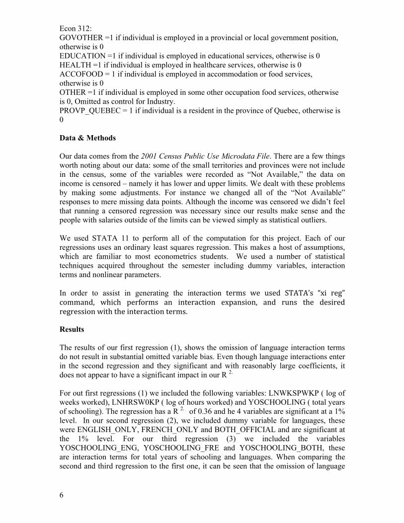
Results The results of our first regression (1), shows the omission of language interaction terms do not result in substantial omitted variable bias. Even though language interactions enter in the second regression and they significant and with reasonably large coefficients, it does not appear to have a significant impact in our R 2.

For out first regressions (1) we included the following variables: LNWKSPWKP ( log of weeks worked), LNHRSW0KP ( log of hours worked) and YOSCHOOLING ( total years of schooling). The regression has a R 2. of 0.36 and he 4 variables are significant at a 1% level. In our second regression (2), we included dummy variable for languages, these were ENGLISH_ONLY, FRENCH_ONLY and BOTH_OFFICIAL and are significant at the 1% level. For our third regression (3) we included the variables YOSCHOOLING_ENG, YOSCHOOLING_FRE and YOSCHOOLING_BOTH, these are interaction terms for total years of schooling and languages. When comparing the second and third regression to the first one, it can be seen that the omission of language

Econ 312:

7

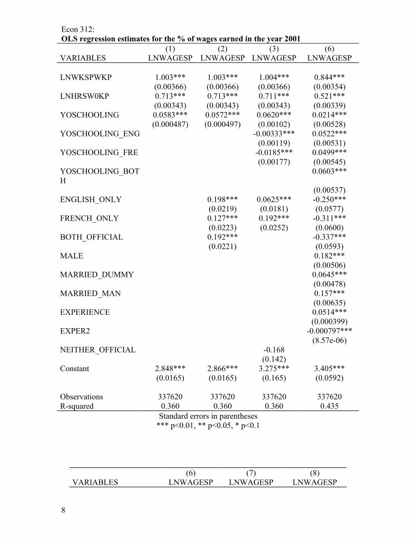
dummy variables and interaction terms do not result in substantial omitted variable bias. Even though all of these new included variables are significant and have reasonably large coefficients, it does not appear to have a significant impact in our R 2.. The R 2. is 0.360 for the three regressions, which means that 36% of the variation in the data is explained through this regression. It is worth noting the coefficient change of the ENGLISH_ONLY variable from the second regression to the third regression. In the second regression the ENGLISH_ONLY variable has a coefficient of 0.198, which is larger than the coefficient for FRENCH_ONLY (0.127), however, in the third regression the coefficient for ENGLISH_ONLY is much smaller (0.0625). We suspect that the reason for this is the addition of the interaction terms, which probably capture part of this effect. It can be seen that the YOSCHOOLING_ENG variable coefficient in the third regression is larger (less negative) than the YOSCHOOLING_FRE variable coefficient. Which goes along with out intuition of English speakers having a higher return to education. To address other potential omitted variables bias, we included other variables besides the ones for education and languages. We included variables that we thought to be relevant in an individual’s potential wage such as gender, marital status and experience (both linear and quadratic form). The results from this fourth regression (4) show that all of the new included variables are significant at a 1% level. The R2 for this regression is 0.435. This is a considerable increase from our past regressions. This shows the importance of including these variable when determining wage. The positive coefficients for MALE, MARRIED_DUMMY, MARRIED_MAN and EXPERIENCE have positive coefficients. These results follow our intuition. Men tend to have higher wages whether because of potential discrimination against women or perhaps as noted by Berndt; women take more time off their career due to maternity leave. Also, it is very reasonable to expect married people (specially men) to have higher wages. The costs of having a “family” motivate individuals to work harder. We ran a fifth (5) and a sixth (6) regression where we included dummy variables for different kinds of industries. We included these variables because we thought that they were relevant to explain wages. The difference between the 2 regressions is our control variable. For the fifth regression we controlled for OTHERINDS and for the sixth regression we controlled for OTHER. However, the meaning of the results was not very different. For example, it can be seen in both that being in the business sector (coefficients of -0.236 and 0.366) is more profitable than being in the agricultural sector (coefficients of -0.827 and -0.255). We tested for the joint significance of the industry variables and they proved to be significant. The R2 for the two regressions was 0.459. Which is an improvement from the fourth regression (0.435).

For our final regression (7), we included the PROVP_QUEBEC dummy variable, to determine the effects of living in Quebec. We previously used the STATA xi command to create interaction terms of PROVP_QUEBEC with all the other variables and ran an F-test. The results of this test lead us to include the PROVP_QUEBEC variable. The coefficient for this variable is -0.0327 and it is significant at a 1% level.

Econ 312:

8

OLS regression estimates for the % of wages earned in the year 2001 (1) (2) (3) (6) VARIABLES LNWAGESP LNWAGESP LNWAGESP LNWAGESP LNWKSPWKP 1.003*** 1.003*** 1.004*** 0.844*** (0.00366) (0.00366) (0.00366) (0.00354) LNHRSW0KP 0.713*** 0.713*** 0.711*** 0.521*** (0.00343) (0.00343) (0.00343) (0.00339) YOSCHOOLING 0.0583*** 0.0572*** 0.0620*** 0.0214*** (0.000487) (0.000497) (0.00102) (0.00528) YOSCHOOLING_ENG -0.00333*** 0.0522*** (0.00119) (0.00531) YOSCHOOLING_FRE -0.0185*** 0.0499*** (0.00177) (0.00545) YOSCHOOLING_BOTH

0.0603***

(0.00537) ENGLISH_ONLY 0.198*** 0.0625*** -0.250*** (0.0219) (0.0181) (0.0577) FRENCH_ONLY 0.127*** 0.192*** -0.311*** (0.0223) (0.0252) (0.0600) BOTH_OFFICIAL 0.192*** -0.337*** (0.0221) (0.0593) MALE 0.182*** (0.00506) MARRIED_DUMMY 0.0645*** (0.00478) MARRIED_MAN 0.157*** (0.00635) EXPERIENCE 0.0514*** (0.000399) EXPER2 -0.000797*** (8.57e-06) NEITHER_OFFICIAL -0.168 (0.142) Constant 2.848*** 2.866*** 3.275*** 3.405*** (0.0165) (0.0165) (0.165) (0.0592) Observations 337620 337620 337620 337620 R-squared 0.360 0.360 0.360 0.435

Standard errors in parentheses *** p<0.01, ** p<0.05, * p<0.1

(6) (7) (8) VARIABLES LNWAGESP LNWAGESP LNWAGESP

Econ 312:

9

LNWKSPWKP 0.832*** 0.832*** 0.832*** (0.00348) (0.00348) (0.00348) LNHRSW0KP 0.486*** 0.486*** 0.486*** (0.00335) (0.00335) (0.00335) YOSCHOOLING 0.0215*** 0.0215*** 0.0214*** (0.00517) (0.00517) (0.00517) YOSCHOOLING_ENG 0.0427*** 0.0427*** 0.0428*** (0.00520) (0.00520) (0.00520) YOSCHOOLING_FRE 0.0416*** 0.0417*** 0.0419*** (0.00533) (0.00533) (0.00533) YOSCHOOLING_BOTH 0.0501*** 0.0501*** 0.0502*** (0.00526) (0.00526) (0.00526) ENGLISH_ONLY -0.200*** -0.200*** -0.203*** (0.0565) (0.0565) (0.0565) FRENCH_ONLY -0.276*** -0.276*** -0.249*** (0.0587) (0.0587) (0.0590) BOTH_OFFICIAL -0.293*** -0.293*** -0.277*** (0.0580) (0.0580) (0.0581) MALE 0.140*** 0.140*** 0.141*** (0.00505) (0.00505) (0.00505) MARRIED_DUMMY 0.0472*** 0.0471*** 0.0471*** (0.00469) (0.00469) (0.00469) MARRIED_MAN 0.156*** 0.156*** 0.156*** (0.00622) (0.00622) (0.00622) EXPERIENCE 0.0446*** 0.0446*** 0.0447*** (0.000396) (0.000396) (0.000396) EXPER2 -0.000686*** -0.000686*** -0.000687*** (8.45e-06) (8.45e-06) (8.45e-06) AGRICULTURE -0.827*** -0.225*** -0.225*** (0.0153) (0.0122) (0.0122) MANUFACTURNG -0.236*** 0.366*** 0.367*** (0.0116) (0.00708) (0.00708) CONSTRUT -0.280*** 0.322*** 0.321*** (0.0127) (0.00886) (0.00886) TRANSSTORAGE -0.289*** 0.313*** 0.313*** (0.0131) (0.00940) (0.00940) COMMUTILITES -0.131*** 0.471*** 0.471*** (0.0138) (0.0102) (0.0102) WHOLESALE -0.274*** 0.328*** 0.329*** (0.0127) (0.00860) (0.00861) RETAIL -0.585*** 0.0164** 0.0164** (0.0119) (0.00723) (0.00723) FINACEREALEST -0.177*** 0.425*** 0.425*** (0.0127) (0.00852) (0.00852) BUSINESS -0.236*** 0.366*** 0.366*** (0.0123) (0.00795) (0.00795) GOVFED -0.0897*** 0.512*** 0.509***

Econ 312:

10

(0.0145) (0.0110) (0.0110) GOVOTHER -0.169*** 0.433*** 0.433*** (0.0135) (0.00972) (0.00972) EDUCATION -0.297*** 0.305*** 0.304*** (0.0125) (0.00807) (0.00807) HEALTH -0.365*** 0.237*** 0.237*** (0.0122) (0.00755) (0.00755) ACCOFOOD -0.728*** -0.126*** -0.126*** (0.0126) (0.00826) (0.00826) OTHER -0.602*** (0.0125) OTHERINDS 0.604*** 0.603*** (0.0126) (0.0126) NEITHER_OFFICIAL PROVP_QUEBEC -0.0327*** (0.00600) Constant 4.121*** 3.519*** 3.521*** (0.0591) (0.0582) (0.0582) Observations 337620 337620 337620 R-squared 0.459 0.459 0.459

When determining the variables to use for our model, we had to look at particular interactions between potentially correlated variables. These interaction terms were studied separately from the models presented above. First, we wanted to determine if our dummy variables for language had any interaction with our YOSCHOOLING variables. Berndt suggested that years of education could be estimated by category since, at least after secondary education, it mostly mattered what kind of degree an individual held rather than total years at school. To test for interaction, we ran a regression using STATA’s “xi“ command to generate dummy variables for our categories with YOSCHOOLING ∗ OLNP as the interaction term.

Econ 312:

11

The joint F-statistic for the joint hypothesis that both the dummy variable for OLNP and the interaction terms are significant is 21456.61, which indicates significance at the 1% level. Most of the YOSCHOOLING dummy variables are significant at the 5% level but the dummies for OLNP and the interaction terms are not significant even at the 10% level. It seems contradictory that the joint F-statistic says the joint hypothesis that the dummies have the same slope and intercept can be rejected but the individual t-statistics

Econ 312:

12

fail to reject it. We can infer that there is a high degree of correlation between the OLNP variable and the interaction terms. Though it is hard to tell which of the coefficients is non-zero, there is strong evidence against the hypothesis that both are zero. Also, the program had dropped YOSCHOOLING terms for 5-7 years of schooling. This is probably due to collinearity among the controlling dummy variables for YOSCHOOLING=5, since there is not much difference for wage for individuals in primary school. This suggests that primary education does not have a significant effect on wages. Also, we had the same thought with our industry variables. We wanted to determine if the effect of schooling depended on what industry you are employed and how should it be controlled for. We then used an xi regression with YOSCHOOLING*IND80P (list of industry by category) as the interaction term. The resulting regression has an overall F-statistic that is significant at the 1% level but determining the significance on individual regressions was difficult. The high standard errors in some of the interaction terms, such as COMMUTILI and GOVFED indicate high correlation between YOSCHOOLING and corresponding industry dummy. It would be safe to assume some industry professions require more schooling than others.

Econ 312:

13

Econ 312:

14

Econ 312:

15

Econ 312:

16

Econ 312:

17

Econ 312:

18

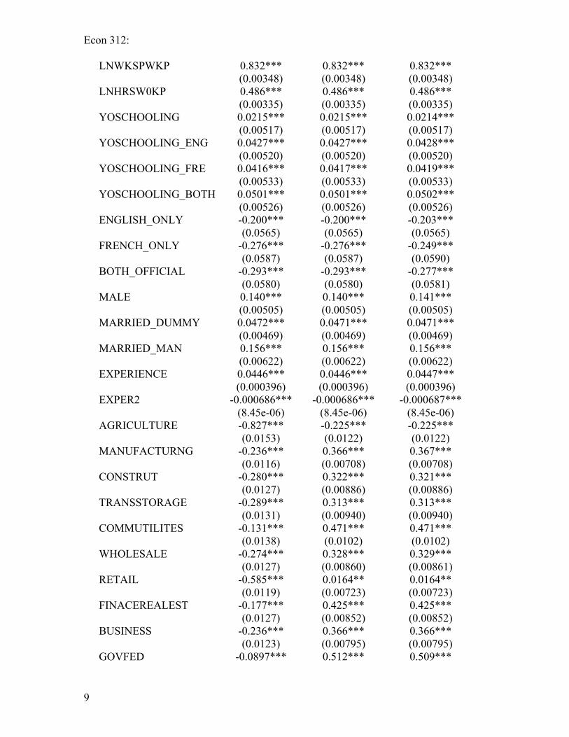
Finally, we tested the interaction of the dummy variable for residence in Quebec and years of schooling. The corresponding xi regression with YOSCHOOLING* PROVP_QUEBEC gave similar responses to the hyposteses as did our OLNP regression. Both terms are highly correlated. We believe that since the population of French speakers in Canada and the population of people in Quebec are nearly identical, it stands to reason that the 2 variables would be directly correlated.

Econ 312:

19

_cons 3.39646 .0287257 118.24 0.000 3.340159 3.452762

_IYOSXPR~5_1 .0701028 .0698018 1.00 0.315 -.0667066 .2069123

_IYOSXP~23_1 .0843622 .0617521 1.37 0.172 -.03667 .2053945

_IYOSXP~19_1 .0581904 .0433305 1.34 0.179 -.0267362 .1431169

_IYOSXP~18_1 .0437302 .0410593 1.07 0.287 -.0367449 .1242052

_IYOSXPR~7_1 .0093045 .0394393 0.24 0.813 -.0679955 .0866045

_IYOSXP~13_1 .0386919 .0401943 0.96 0.336 -.0400878 .1174716

_IYOSXPR~2_1 .0722234 .0402305 1.80 0.073 -.0066272 .151074

_IYOSXPR~1_1 .1251912 .0411471 3.04 0.002 .0445441 .2058384

_IYOSXPR~0_1 .0425975 .0423435 1.01 0.314 -.0403946 .1255895

_IYOSXP~_9_1 .0431895 .0443842 0.97 0.331 -.0438023 .1301812

_IYOSXP~_8_1 .0210799 .0434024 0.49 0.627 -.0639876 .1061475

_IPROVP_QU~1 -.0674575 .0389126 -1.73 0.083 -.1437251 .0088102

_IYOSCHOO~25 .832733 .0375325 22.19 0.000 .7591703 .9062956

_IYOSCHOO~23 .9323936 .0328408 28.39 0.000 .8680266 .9967606

_IYOSCHOO~19 .7919572 .0257475 30.76 0.000 .7414927 .8424216

_IYOSCHOO~18 .5882323 .0252187 23.33 0.000 .5388044 .6376602

_IYOSCHOO~17 .4490066 .0243441 18.44 0.000 .4012929 .4967202

_IYOSCHOO~13 .1940319 .0247737 7.83 0.000 .1454761 .2425876

_IYOSCHOO~12 .1707191 .0244331 6.99 0.000 .122831 .2186071

_IYOSCHOO~11 .0489081 .0252924 1.93 0.053 -.0006642 .0984804

_IYOSCHOO~10 .0743335 .0253633 2.93 0.003 .024622 .1240449

_IYOSCHOO~_9 .0559024 .0272835 2.05 0.040 .0024276 .1093773

_IYOSCHOO~_8 .0922048 .0269003 3.43 0.001 .039481 .1449287

LNHRSW0KP .7070666 .003428 206.26 0.000 .7003479 .7137854

LNWKSPWKP 1.00266 .0036587 274.05 0.000 .9954888 1.009831

LNWAGESP Coef. Std. Err. t P>|t| [95% Conf. Interval]

Total 461531.455337619 1.36701861 Root MSE = .93346

Adj R-squared = 0.3626

Residual 294160.017337594 .871342549 R-squared = 0.3626

Model 167371.439 25 6694.85754 Prob > F = 0.0000

F( 25,337594) = 7683.38

Source SS df MS Number of obs = 337620

i.Y~ING*i.PRO~C _IYOSXPRO_#_# (coded as above)

i.PROVP_QUEBEC _IPROVP_QUE_0-1 (naturally coded; _IPROVP_QUE_0 omitted)

i.YOSCHOOLING _IYOSCHOOLI_5-25 (naturally coded; _IYOSCHOOLI_5 omitted)

. xi:reg LNWAGESP LNWKSPWKP LNHRSW0KP i.YOSCHOOLING*i.PROVP_QUEBEC

Econ 312:

20

Concluding remarks Summary of model results Language known change in Earnings (LNWAGE)

outside Quebec for an additional year of school

change in Earnings (LNWAGE) in Quebec for an additional year of school

English 0.642 0.315 French 0.633 0.306 Both Languagues 0.726 0.395

When examining the results of these regressions, it is clear that the interaction terms for years of schooling and language always show a higher coefficient for the English speakers than for French speakers. It is also worth mentioning the negative coefficient for the Quebec province dummy variable. It can be argued that this variable works as a proxy for French speakers (considering the demographics of Quebec). Taking all of this evidence into account, it can be concluded that the returns to education are higher for English speakers than for French speakers.

It is hard to know all the factors that lead to this language “discrimination”. Perhaps, the most important reason for this difference is that English speakers are the majority in Canada (roughly 80% against 20% French). This is a reason for employers to hire English speakers rather than French speakers. In addition, there are a higher percentage of native French speakers that speak English than native English speakers that speak French. This reinforces the relevance of English. Since Canada is 80% English, this likely increases the chances of getting a job in an English-speaking city (such as Toronto, Vancouver, Calgary, etc).