Retiring Adult: New Datasets for Fair Machine Learning

Retiring Adult: New Datasets for Fair Machine Learning

Frances Ding∗

UC BerkeleyMoritz Hardt∗

UC BerkeleyJohn Miller∗

UC BerkeleyLudwig Schmidt∗

Toyota Research Institute

Abstract

Although the fairness community has recognized the importance of data, researchers in thearea primarily rely on UCI Adult when it comes to tabular data. Derived from a 1994 US Censussurvey, this dataset has appeared in hundreds of research papers where it served as the basis forthe development and comparison of many algorithmic fairness interventions. We reconstructa superset of the UCI Adult data from available US Census sources and reveal idiosyncrasiesof the UCI Adult dataset that limit its external validity. Our primary contribution is a suiteof new datasets derived from US Census surveys that extend the existing data ecosystem forresearch on fair machine learning. We create prediction tasks relating to income, employment,health, transportation, and housing. The data span multiple years and all states of the UnitedStates, allowing researchers to study temporal shift and geographic variation. We highlighta broad initial sweep of new empirical insights relating to trade-offs between fairness criteria,performance of algorithmic interventions, and the role of distribution shift based on our newdatasets. Our findings inform ongoing debates, challenge some existing narratives, and point tofuture research directions.

1 Introduction

Datasets are central to the machine learning ecosystem. Besides providing training and testingdata for model builders, datasets formulate problems, organize communities, and interface betweenacademia and industry. Influential works relating to the ethics and fairness of machine learningrecognize the centrality of datasets, pointing to significant harms associated with data, as well asbetter data practices [11, 17, 21, 25, 27]. While the discourse about data has prioritized cognitivedomains such as vision, speech, or language, numerous consequential applications of predictivemodeling and risk assessment involve bureaucratic, organizational, and administrative records bestrepresented as tabular data [8, 15, 26].

When it comes to tabular data, surprisingly, most research papers on algorithmic fairness continue toinvolve a fairly limited collection of datasets, chief among them the UCI Adult dataset [22]. Derivedfrom the 1994 Current Population Survey conducted by the US Census Bureau, this dataset hasmade an appearance in more than three hundred research papers related to fairness where it servedas the basis for the development and comparison of many algorithmic fairness interventions.

Our work begins with a critical examination of the UCI Adult dataset—its origin, impact, andlimitations. To guide this investigation we identify the previously undocumented exact source of

∗Authors ordered alphabetically

1

arX

iv:2

108.

0488

4v2

[cs

.LG

] 1

8 O

ct 2

021

the UCI Adult dataset, allowing us to reconstruct a superset of the data from available US Censusrecords. This reconstruction reveals a significant idiosyncrasy of the UCI Adult prediction task thatlimits its external validity.

While some issues with UCI Adult are readily apparent, such as its age, limited documentation, andoutdated feature encodings, a significant problem may be less obvious at first glance. Specifically,UCI Adult has a binary target label indicating whether the income of a person is greater or lessthan fifty thousand US dollars. This income threshold of $50k US dollars corresponds to the 76thquantile of individual income in the United States in 1994, the 88th quantile in the Black population,and the 89th quantile among women. We show how empirical findings relating to algorithmicfairness are sensitive to the choice of the income threshold, and how UCI Adult exposes a ratherextreme threshold. Specifically, the magnitude of violations in different fairness criteria, trade-offsbetween them, and the effectiveness of algorithmic interventions all vary significantly with the incomethreshold. In many cases, the $50k threshold understates and misrepresents the broader picture.

Turning to our primary contribution, we provide a suite of new datasets derived from US Censusdata that extend the existing data ecosystem for research on fair machine learning. These datasetsare derived from two different data products provided by the US Census Bureau. One is the PublicUse Microdata Sample of the American Community Survey, involving millions of US householdseach year. The other is the Annual Social and Economic Supplement of the Current PopulationSurvey. Both released annually, they represent major surveying efforts of the Census Bureau thatare the basis of important policy decisions, as well as vital resources for social scientists.

We create prediction tasks in different domains, including income, employment, health, transportation,and housing. The datasets span multiple years and all states of the United States, in particular,allowing researchers to study temporal shift and geographic variation. Alongside these predictiontasks, we release a Python package called folktables which interfaces with Census data sourcesand allows users to both access our new predictions tasks and create new tasks from Census datathrough a simple API1.

We contribute a broad initial sweep of new empirical insights into algorithmic fairness based on ournew datasets. Our findings inform ongoing debates and in some cases challenge existing narrativesabout statistical fairness criteria and algorithmic fairness interventions. We highlight three robustobservations:

1. Variation within the population plays a major role in empirical observations and how theyshould be interpreted:

(a) Fairness criteria and the effect size of different interventions varies greatly by state. Thisshows that statistical claims about algorithmic fairness must be qualified carefully bycontext, even though they often are not.

(b) Training on one state and testing on another generally leads to unpredictable results.Accuracy and fairness criteria could change in either direction. This shows that algorithmictools developed in one context may not transfer gracefully to another.

(c) Somewhat surprisingly, fairness criteria appear to be more stable over time than predictiveaccuracy. This is true both before and after intervention.

1The datasets and Python package are available for download at https://github.com/zykls/folktables.

2

https://github.com/zykls/folktables

2. Algorithmic fairness interventions must specify a locus of intervention. For example, a modelcould be trained on the entire US population, or on a state-by-state basis. The results differsignificantly. Recognition of the need for such a choice is still lacking, as is scholarship guidingthe practitioner on how to navigate this choice and its associated trade-offs.

3. Increased dataset size does not necessarily help in reducing observed disparities. Neither doessocial progress as measured in years passed. This is in contrast to intuition from cognitivemachine learning tasks where more representative data can improve metrics such as error ratedisparities between different groups.

Our observations apply to years of active research into algorithmic fairness, and our work providesnew datasets necessary to re-evaluate and extend the empirical foundations of the field.

2 Archaeology of UCI Adult: Origin, Impact, LimitationsArchaeology organises the past to understand the present. It lifts the dust-cover off a world that we takefor granted. It makes us reconsider what we experience as inevitable.

— Ian Hacking

Although taken for granted today, the use of benchmark datasets in machine learning emergedonly in late 1980s [19]. Created in 1987, the UCI Machine Learning Repository contributed to thisdevelopment by providing researchers with numerous datasets each with a fixed training and testingsplit [23]. As of writing, the UCI Adult dataset is the second most popular dataset among morethan five hundred datasets in the UCI repository. An identical dataset is called “Census IncomeData Set” and a closely related larger dataset goes by “Census-Income (KDD) Data Set”.

At the outset, UCI Adult contains 48,842 rows each apparently describing one individual with 14attributes. The dataset information reveals that it was extracted from the “1994 Census database”according to certain filtering criteria. Since the US Census Bureau provides several data products,as we will review shortly, this piece of information does not identify the source of the dataset.

The fourteen features of UCI Adult include what the fairness community calls sensitive or protectedattributes, such as, age, sex, and race. The earliest paper on algorithmic fairness that used UCIAdult to our knowledge is a work by Calders et al. [12] from 2009. The availability of sensitiveattributes contributed to the choice of the dataset for the purposes of this work. An earlier paper inthis context by Pedreschi et al. [29] used the UCI German credit dataset, which is smaller and endedup being less widely used in the community. Another highly cited paper on algorithmic fairnessthat popularized UCI Adult is the work of Zemel et al. [34] on learning fair representations (LFR).Published in 2013, the work introduced the idea of changing the data representation to achieve aparticular fairness criterion, in this case, demographic parity, while representing the original data aswell as possible. This idea remains popular in the community and the LFR method has become astandard baseline.

Representation learning is not the only topic for which UCI Adult became the standard test case.The dataset has become broadly used throughout the area for purposes including the developmentof new fairness criteria, algorithmic interventions and fairness promoting methods, as well as causalmodeling. Major software packages, such as AI Fairness 360 [7] and Fairlearn [9], expose UCI Adultas one of a few standard examples. Indeed, based on bibliographic information available on Google

3

Scholar there appear to be more than 300 papers related to algorithmic fairness that used the UCIAdult dataset at the time of writing.

2.1 Reconstruction of UCI Adult

Creating a dataset involves a multitude of design choices that substantially affect the validity ofexperiments conducted with the dataset. To fully understand the context of UCI Adult and explorevariations of its design choices, we reconstructed a closely matching superset from the original Censussources. We now describe our reconstruction in detail and then investigate one specific design choice,the income binarization threshold, in Section 2.2.

The first step in our reconstruction of UCI Adult was identifying the original data source. Asmentioned above, the “1994 census database“ description in the UCI Adult documentation does notuniquely identify the data product provided by the US Census Bureau. Based on the documentationof the closely related “Census-Income (KDD) Data Set,”2 we decided to start with the CurrentPopulation Survey (CPS) data, specifically the Annual Social and Economic Supplement (ASEC)from 1994. We utilized the IPUMS interface to the CPS data [16] and hence refer to our reconstructionas IPUMS Adult.

The next step in the reconstruction was matching the 15 features in UCI Adult to the CPS data.This was a non-trivial task: the UCI Adult documentation does not mention any specific CPSvariable names and IPUMS CPS contains more than 400 candidate variables for the 1994 ASEC.To address this challenge, we designed the following matching procedure that we repeated for eachfeature in UCI Adult: First, identify a set of candidate variables in CPS via the IPUMS keywordsearch. For each candidate variable, use the CPS documentation to manually derive a mapping fromthe CPS encoding to the UCI Adult encoding. Finally, match each row in UCI Adult to its nearestneighbor in the partial reconstruction assembled from previous exact variable matches.

We only included a candidate variable if the nearest neighbor match was exact, i.e., we could find anexact match in the IPUMS CPS data for each row in UCI Adult that matched both the candidatevariable and all earlier variables also identified via exact matches. There were only two exceptions tothis rule. We discuss them in Appendix A. After completing the variable matching, our reconstructionhas 49,531 rows when we use the same inclusion criteria as UCI Adult to the extent possible, whichis slightly more than the 48,842 rows in UCI Adult. The discrepancy likely stems from the fact thatUCI Adult used the variable “fnlwgt” in its inclusion criteria and we did not due to the lack of anexact match for this variable. This made our inclusion criteria slightly more permissive than thoseof UCI Adult. The fact that we found exact matches for 13 of the 15 UCI Adult variables and avery close match for “native-country” is evidence that our reconstruction of UCI Adult is accurate.

2.2 Varying income threshold

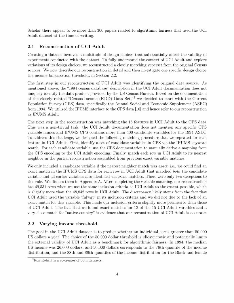
The goal in the UCI Adult dataset is to predict whether an individual earns greater than 50,000US dollars a year. The choice of the 50,000 dollar threshold is idiosyncratic and potentially limitsthe external validity of UCI Adult as a benchmark for algorithmic fairness. In 1994, the medianUS income was 26,000 dollars, and 50,000 dollars corresponds to the 76th quantile of the incomedistribution, and the 88th and 89th quantiles of the income distribution for the Black and female

2Ron Kohavi is a co-creator of both datasets.

4

20000 40000 60000Income threshold

0.65

0.70

0.75

0.80

0.85

0.90

0.95

1.00

Accu

racy

IPUMS Adult


0.0

0.1

0.2

0.3

0.4

P(Y

=1

Mal

e)P(

Y=

1Fe

mal

e)

Demographic parity (DP) violation


0.2

0.1

0.0

0.1

0.2

0.3

0.4

P(Y

=1

Mal

e,Y

=1)

P(Y

=1

Fem

ale,

Y=

1)

Equality of opportunity (EO) violation

GBM GBM w / LFR GBM w/ Postprocessing (DP) GBM w/ ExpGrad (DP) UCI Adult threshold

Figure 1: Fairness interventions with varying income threshold on IPUMS Adult. We comparethree methods for achieving demographic parity: a pre-processing method (LFR), an in-trainingmethod based on Agarwal et al. [2] (ExpGrad), and a post-processing adjustment method [20]. Weapply each method using a gradient boosted decision tree (GBM) as the base classifier. Confidenceintervals are 95% Clopper-Pearson intervals for accuracy and 95% Newcombe intervals for DP.

populations, respectively. Consequently, almost all of the Black and female instances in the datasetfall below the threshold and models trained on UCI adult tend to have substantially higher accuracieson these subpopulations. For instance, a standard logistic regression model trained on UCI Adultdataset achieves 85% accuracy overall, 91.4% accuracy on the Black instances, and 92.7% on Femaleinstances. This is a rather untypical situation since often machine learning models perform morepoorly on historically disadvantaged groups.

To understand the sensitivity of the empirical findings on UCI Adult to the choice of threshold, weleverage our IPUMS Adult reconstruction, which includes the continuous, unthresholded incomevariable, and construct a new collection of datasets where the income threshold varies from 6,000 to70,000. For each threshold, we first train a standard gradient boosted decision tree and evaluateboth its accuracy and its violation of two common fairness criteria: demographic parity (equalityof positive rates) and equal opportunity (equality of true positive rates). See the text by Barocaset al. [6] for background. The results are presented in Figure 1, where we see both accuracy and themagnitude of violations of these criteria vary substantially with the threshold choice.

We then evaluate how the choice of threshold affects three common classes of fairness interventions:the preprocessing method LFR [34] mentioned earlier, an in-processing or in-training method basedon the reductions approach in Agarwal et al. [2], and the post-processing method from Hardt et al.[20]. In Figure 1, we plot model accuracy after applying each intervention to achieve demographicparity as well as violations of both demographic parity and equality of opportunity as the incomethreshold varies. In Appendix A, we conduct the same experiment for methods to achieve equalityof opportunity. There are three salient findings. First, the effectiveness of each intervention dependson the threshold. For values of the threshold near 25,000, the accuracy drop needed to achievedemographic parity or equal opportunity is significantly larger than closer to 50,000. Second, thetrade-offs between different criteria vary substantially with the threshold. Indeed, for the in-processingmethod enforcing demographic parity, as the threshold varies, the equality of opportunity violationis monotonically increasing. Third, for high values of the threshold, the small number of positiveinstances substantially enlarges the confidence intervals for equality of opportunity, which makes it

5

Table 1: New prediction task details instantiated on 2018 US-wide ACS PUMS data

Task Features Datapoints Constantpredictor acc LogReg acc GBM acc

ACSIncome 10 1,599,229 63.1% 77.1% 79.7%ACSPublicCoverage 19 1,127,446 70.2% 75.6% 78.5 %ACSMobility 21 620,937 73.6% 73.7% 75.7%ACSEmployment 17 2,320,013 56.7% 74.3% 78.5%ACSTravelTime 16 1,428,642 56.3% 57.4% 65.0%

difficult to meaningfully compare the performance of methods for satisfying this constraint.

3 New datasets for algorithmic fairness

At least one aspect of UCI Adult is remarkably positive. The US Census Bureau invests heavilyin high quality data collection, surveying methodology, and documentation based on decades ofexperience. Moreover, responses to some US Census Bureau surveys are legally mandated andhence enjoy high response rates resulting in a representative sample. In contrast, some notabledatasets in machine learning are collected in an ad-hoc manner, plagued by skews in representation[10, 13, 32, 33], often lacking copyright [24] or consent from subjects [30], and involving unskilled orpoorly compensated labor in the form of crowd workers [18].

In this work, we tap into the vast data ecosystem of the US Census Bureau to create new machinelearning tasks that we hope help to establish stronger empirical evaluation practices within thealgorithmic fairness community.

As previously discussed, UCI Adult was derived from the Annual Social and Economic Supplement(ASEC) of the Current Population Survey (CPS). The CPS is a monthly survey of approximately60,000 US households. It’s used to produce the official monthly estimates of employment andunemployment for the United States. The ASEC contains additional information collected annually.

Another US Census data product most relevant to us are the American Community Survey (ACS)Public Use Microdata Sample (PUMS). ACS PUMS differs in some significant ways from CPS ASEC.The ACS is sent to approximately 3.5 million US households each year gathering information relatingto ancestry, citizenship, education, employment, language proficiency, income, disability, and housingcharacteristics. Participation in the ACS is mandatory under federal law. Responses are confidentialand governed by strict privacy rules. The Public Use Microdata Sample contains responses to everyquestion from a subset of respondents. The geographic information associated with any given recordis limited to a level that aims to prevent re-identification of survey participants. A number of otherdisclosure control heuristics are implemented. Extensive documentation is available on the websitesof the US Census Bureau.

3.1 Available prediction tasks

We use ACS PUMS as the basis for the following new prediction tasks:

6

ACSIncome: predict whether an individual’s income is above $50,000, after filtering the ACSPUMS data sample to only include individuals above the age of 16, who reported usual workinghours of at least 1 hour per week in the past year, and an income of at least $100. The threshold of$50,000 was chosen so that this dataset can serve as a replacement to UCI Adult, but we also offerdatasets with other income cutoffs described in Appendix B.

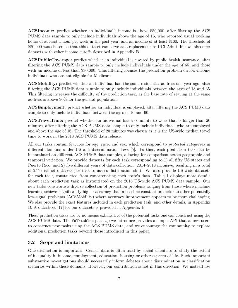
ACSPublicCoverage: predict whether an individual is covered by public health insurance, afterfiltering the ACS PUMS data sample to only include individuals under the age of 65, and thosewith an income of less than $30,000. This filtering focuses the prediction problem on low-incomeindividuals who are not eligible for Medicare.

ACSMobility: predict whether an individual had the same residential address one year ago, afterfiltering the ACS PUMS data sample to only include individuals between the ages of 18 and 35.This filtering increases the difficulty of the prediction task, as the base rate of staying at the sameaddress is above 90% for the general population.

ACSEmployment: predict whether an individual is employed, after filtering the ACS PUMS datasample to only include individuals between the ages of 16 and 90.

ACSTravelTime: predict whether an individual has a commute to work that is longer than 20minutes, after filtering the ACS PUMS data sample to only include individuals who are employedand above the age of 16. The threshold of 20 minutes was chosen as it is the US-wide median traveltime to work in the 2018 ACS PUMS data release.

All our tasks contain features for age, race, and sex, which correspond to protected categories indifferent domains under US anti-discrimination laws [5]. Further, each prediction task can beinstantiated on different ACS PUMS data samples, allowing for comparison across geographic andtemporal variation. We provide datasets for each task corresponding to 1) all fifty US states andPuerto Rico, and 2) five different years of data collection: 2014–2018 inclusive, resulting in a totalof 255 distinct datasets per task to assess distribution shift. We also provide US-wide datasetsfor each task, constructed from concatenating each state’s data. Table 1 displays more detailsabout each prediction task as instantiated on the 2018 US-wide ACS PUMS data sample. Ournew tasks constitute a diverse collection of prediction problems ranging from those where machinelearning achieves significantly higher accuracy than a baseline constant predictor to other potentiallylow-signal problems (ACSMobility) where accuracy improvement appears to be more challenging.We also provide the exact features included in each prediction task, and other details, in AppendixB. A datasheet [17] for our datasets is provided in Appendix E.

These prediction tasks are by no means exhausitive of the potential tasks one can construct using theACS PUMS data. The folktables package we introduce provides a simple API that allows usersto construct new tasks using the ACS PUMS data, and we encourage the community to exploreadditional prediction tasks beyond those introduced in this paper.

3.2 Scope and limitations

One distinction is important. Census data is often used by social scientists to study the extentof inequality in income, employment, education, housing or other aspects of life. Such importantsubstantive investigations should necessarily inform debates about discrimination in classificationscenarios within these domains. However, our contribution is not in this direction. We instead use

7

0.78 0.80 0.82 0.84State accuracy

0.0

0.1

0.2

0.3P(

Y=

1W

hite

)P(

Y=

1Bl

ack) GBM w/ LFR

0.78 0.80 0.82 0.84State accuracy

0.0

0.1

0.2

0.3GBM w/ ExpGrad (DP)

0.78 0.80 0.82 0.84State accuracy

0.0

0.1

0.2

0.3GBM w/ Post-processing (DP)

AL CA HI IN ME MI NM NY WA

Figure 2: The effect size of fairness interventions varies by state. Each panel shows the change inaccuracy and demographic parity on the ACSIncome task after applying a fairness intervention toan unconstrained gradient boosted decision tree (GBM). Each arrow corresponds to a different statedistribution. The arrow base represents the (accuracy, DP) point corresponding to the unconstrainedGBM, and the head represents the (accuracy, DP) point obtained after applying the intervention.The arrow for HI in the LFR plot is entirely covered by the start and end points.

census data for the empirical study of algorithmic fairness. This generally may include performanceclaims about specific methods, the comparison of different methods for achieving a given fairnessmetric, the relationships of different fairness criteria in concrete settings, causal modeling of differentscenarios, and the ability of different methods to transfer successfully from one context to another.We hope that our work leads to more comprehensive empirical evaluations in research papers onthe topic, at the very least reducing the overreliance on UCI Adult and providing a complementto the flourishing theoretical work on the topic. The distinction we draw between benchmark dataand substantive domain-specific investigations resonates with recent work that points out issueswith using data about risk assessments tools from the criminal justice domain as machine learningbenchmarks [4].

A notable if obvious limitation of our work is that it is entirely US-centric. A richer dataset ecosystemcovering international contexts within the algorithmic fairness community is still lacking. Althoughempirical work in the Global South is central in other disciplines, there continues to be much needfor the North American fairness community to engage with it more strongly [1].

4 A tour of empirical observations

In this section, we highlight an initial sweep of empirical observations enabled by our new ACS PUMSderived prediction tasks. Our experiments focus on three fundamental issues in fair machine learning:(i) variation within the population of interest, e.g., how does the effectiveness of interventions varybetween different states or over time?, (ii) the locus of intervention, e.g. should interventions beperformed at the state or national level?, and (iii) whether increased dataset size or the passage oftime mitigates observed disparities?

Our experiments are not exhaustive and are intended to highlight the perspective a broader empiricalevaluation with our new datasets can contribute to addressing questions within algorithmic fairness.The goal of the experiments is not to provide a complete overview of all the questions that one can

8

0.65 0.70 0.75 0.80 0.85Accuracy

0.1

0.0

0.1

0.2

0.3

0.4

P(Y

=1

Whi

te)

P(Y

=1

Blac

k) GBM, train on CAID (CA) evaluationOOD evaluation

0.65 0.70 0.75 0.80 0.85Accuracy

0.1

0.0

0.1

0.2

0.3

0.4GBM, train on TX

ID (TX) evaluationOOD evaluation

0.65 0.70 0.75 0.80 0.85Accuracy

0.1

0.0

0.1

0.2

0.3

0.4GBM, train on IN

ID (IN) evaluationOOD evaluation

0.65 0.70 0.75 0.80 0.85Accuracy

0.1

0.0

0.1

0.2

0.3

0.4GBM, train on NY

ID (NY) evaluationOOD evaluation

ACSIncome 2018 1-Year

0.65 0.70 0.75 0.80 0.85Accuracy

0.1

0.0

0.1

0.2

0.3

0.4

P(Y

=1

Whi

te)

P(Y

=1

Blac

k) Postprocess (DP) on CAID (CA) evaluationOOD evaluation

0.65 0.70 0.75 0.80 0.85Accuracy

0.1

0.0

0.1

0.2

0.3

0.4

Postprocess (DP) on TXID (TX) evaluationOOD evaluation

0.65 0.70 0.75 0.80 0.85Accuracy

0.1

0.0

0.1

0.2

0.3

0.4

Postprocess (DP) on INID (IN) evaluationOOD evaluation

0.65 0.70 0.75 0.80 0.85Accuracy

0.1

0.0

0.1

0.2

0.3

0.4

Postprocess (DP) on NYID (NY) evaluationOOD evaluation

Figure 3: Transfer from one state to another gives unpredictable results in terms of predictiveaccuracy and fairness criteria. Top: Each panel shows an unconstrained GBM trained on a particularstate on the ACSIncome task and evaluated both in-distribution (ID) on the same state and out-of-distribution (OOD) on the 49 other states in terms of accuracy and demographic parity violation.Bottom: Each panel shows an GBM with post-processing to enforce demographic parity on thestate on which it was trained and evaluated both ID and OOD on all 50 states. Confidence intervalsare 95% Clopper-Pearson intervals for accuracy and 95% Newcombe intervals for demographic parity.

answer using our datasets. Rather, we hope to inspire other researchers to creatively use our datasetsto further probe these question as well as propose new ones leveraging the ACS PUMS data.

4.1 Variation within the population

The ACS PUMS prediction tasks present two natural axes of variation: geographic variation betweenstates and temporal variation between years the ACS is conducted. This variation allows us toboth measure the performance of different fairness interventions on a broad collection of differentdistributions, as well as study the performance of these interventions under geographical and temporaldistribution shift when the test dataset differs from the one on which the model was trained.

Due to space constraints, we focus our experiments in this section on the ACSIncome predictiontask with demographic parity as the fairness criterion of interest. We present similar results for ourother prediction tasks and fairness criteria, as well as full experimental details in Appendix D.

Intervention effect sizes vary across states. The fifty US states which comprise the ACSPUMS data present a broad set of different experimental conditions on which to evaluate theperformance of fairness interventions. At the most basic level, we can train and evaluate differentfairness interventions on each of the states and compare the interventions’ efficacy on these different

9

distributions. Concretely, we first train an unconstrained gradient boosted decision tree (GBM)on each state, and we compare the accuracy and fairness criterion violation of this unconstrainedmodel with the same model after applying one of three common fairness intervention: pre-processing(LFR), the in-processing fair reductions methods from Agarwal et al. [2] (ExpGrad), and the simplepost-processing method that adjusts group-based acceptance thresholds to satisfy a constraint [20].Figure 2 shows the result of this experiment for the ACSIncome prediction task for interventions toachieve demographic parity. For a given method, performance can differ markedly between states.For instance, LFR decreases the demographic parity violation by 10% in some states and in otherstates the decrease is close to zero. Similarly, the post-processing adjustment to enforce demographicparity incurs accuracy drops of less than 1% in some states, whereas in others the drop is closer to5%.

Training and testing on different states leads to unpredictable results. Beyond trainingand evaluating interventions on different states, we also use the ACS PUMS data to study theperformance of interventions under geographic distribution shift, where we train a model on onestate and test it on another. In Figure 3, we plot accuracy and demographic parity violation withrespect to race for both an unconstrained GBM and the same model after applying a post-processingadjustment to achieve demographic parity on a natural suite of test sets: the in-distribution (samestate test set) and the out-of-distribution test sets for the 49 other states. For both the unconstrainedand post-processed model, model accuracy and demographic parity violation varies substantiallyacross different state test sets. In particular, even when a method achieves demographic parity inone state, it may no longer satisfy the fairness constraint when naively deployed on another.

Fairness criteria are more stable over time than predictive accuracy. In contrast tothe unpredictable results that occur under geographic distribution shift, the fairness criteria andinterventions we study are much more stable under temporal distribution shift. Specifically, inFigure 4, we plot model accuracy and demographic parity violation for GBM trained on theACSIncome task using US-wide data from 2014 and evaluated on the test sets for the same taskdrawn from years 2014-2018. Perhaps unsurprisingly, model accuracy degrades slightly over time.However, the associated fairness metric is stable and essentially constant over time. Moreover, thissame trend holds for the fairness interventions previously discussed. The same base GBM withpre-processing (LFR), in-processing (ExpGrad), or post-processing to satisfy demographic parity in2014, all have a similar degradation in accuracy, but the fairness metrics remain stable. Thus, aclassifier that satisfies demographic parity on the 2014 data continues to satisfy the constraint on2015-2018 data.

4.2 Specifying a locus of intervention

On the ACSPUMs prediction task, fairness interventions can be applied either on a state-by-statebasis or on the entire US population. In Table 2, we compare the performance of LFR and thepost-processing adjustment method applied at the US-level with the aggregate performance of bothmethods applied on a state-by-state basis, using a GBM as the base classifier. In both cases, applyingthe intervention on a state-by-state improves US-wide accuracy while still preserving demographicparity (post-processing) or further mitigating violations of demographic parity (LFR).

10

2014 2015 2016 2017 2018Evaluation year

0.76

0.78

0.80

0.82

0.84

0.86

Accu

racy

2014 2015 2016 2017 2018Evaluation year

0.000

0.025

0.050

0.075

0.100

0.125

0.150

0.175

P(Y

=1

Whi

te)

P(Y

=1

Blac

k)

ACSIncome US-Wide (Trained on 2014 data)

GBM GBM w/ ExpGrad (DP) GBM w/ Postprocessing (DP) GBM w/ LFR

Figure 4: Fairness criteria are more stable over time than accuracy. Left: Models trained in 2014on US-wide ACSIncome with and without fairness interventions to achieve demographic parity andevaluated on data in subsequent years suffer a drop in accuracy over time. Right: However, theviolation of demographic parity remains essentially constant over time. Confidence intervals are 95%Clopper-Pearson intervals for accuracy and 95% Newcombe intervals for demographic parity.

Table 2: Comparison of two different strategies for applying an intervention to achieve demographicparity (DP) on the US-wide ACSIncome task. US-level corresponds to training one classifier andapplying the intervention on the entire US population. State-level corresponds to training a classifierand applying the intervention separately for each state and then aggregating the results over allstates. Here, DP refers to P (Y = 1 | White) − P (Y = 1 | Black). Confidence intervals are 95%Clopper-Pearson intervals for accuracy and 95% Newcombe intervals for DP.

US-level acc US-levelDP violation State-level acc State-level

DP violation

Unconstrained GBM 81.7± 0.1 % 17.7± 0.2% 82.8± 0.1 % 16.9± 0.2%GBM w/ LFR 78.7± 0.1 % 16.6± 0.2% 79.4± 0.1% 14.0± 0.2%GBM w/ post-processing (DP) 79.2± 0.1 % 0.3± 0.3 % 80.2± 0.1% −0.6± 0.3%

11

Table 3: Disparities persist despite increasing dataset size and social progress.Dataset Year Datapoints GBM acc TPR White TPR Black TPR disparity

IPUMS Adult 1994 49,531 86.4% 58.0% 46.5 % 11.5%ACSIncome 2018 1,599,229 80.8% 66.5% 51.7% 14.8%

4.3 Increased dataset size doesn’t necessarily mitigate observed disparities

To mitigate disparities in error rates, commonly suggested remedies include collecting a) largerdatasets and b) more representative data reflective of social progress. For example, in responseto research revealing the stark accuracy disparities of commercial facial recognition algorithms,particularly for dark-skinned females [11], IBM collected a more diverse training set of images,retrained its facial recognition model, and reported a 10-fold decrease in error for this subgroup [31].However, on our tabular datasets, larger datasets collected in more socially progressive times do notautomatically mitigate disparities. Table 3 shows that unconstrained gradient boosted decision treetrained on a newer, larger dataset (ACSIncome vs. IPUMS Adult), does not improve disparitiessuch as in true positive rate (TPR). A fundamental reason for this is the persistent social inequalitythat is reflected in the data. It is well known that given a disparity in base rates between groups, apredictive model cannot be both calibrated and equal in error rates across groups [14], except if themodel has 100% accuracy. This observation highlights a key difference between cognitive machinelearning and tabular data prediction – the Bayes error rate is zero for cognitive machine learning.Thus larger and more representative datasets eventually address disparities by pushing error rates tozero for all subgroups. In the tabular datasets we collect, the Bayes error rate of an optimal classifieris almost certainly far from zero, so some individuals will inevitably be incorrectly classified. Ratherthan hope for future datasets to implicitly address disparities, we must directly contend with howdataset and model design choices distribute the burden of these errors.

5 Discussion and future directions

Rather than settled conclusions, our empirical observations are intended to spark additional workon our new datasets. Of particular interest is a broad and comprehensive evaluation of existingmethods on all datasets. We only evaluated some methods so far. One interesting question is ifthere is a method for achieving either demographic parity or error rate parity that outperformsthreshold adjustment (based on the best known unconstrained classifier) on any of our datasets?We conjecture that the answer is no. The reason is that we believe on our datasets a well-tunedtree-ensemble achieves classification error close to the Bayes error bound. Existing theory (Theorem5.3 in [20]) would then show that threshold adjustment based on this model is, in fact, optimal. Ourconjecture motivates drawing a distinction between classification scenarios where a nearly Bayesoptimal classifier is known and those where there isn’t. How close we are to Bayes optimal on any ofour new prediction tasks is a good question. The role of distribution shift also deserves more attention.Are there methods that achieve consistent performance across geographic contexts? Why does thereappear to be more temporal than geographic stability? What does the sensitivity to distributionshift say about algorithmic tools developed in one context and deployed in another? Answers tothese questions seem highly relevant to policy-making around the deployment of algorithmic riskassessment tools. Finally, our datasets are also interesting test cases for causal inference methods,

12

which we haven’t yet explored. How would, for example, methods like invariant risk minimization[3] perform on different geographic contexts?

Acknowledgements

We thank Barry Becker and Ronny Kohavi for answering our many questions around the origin andcreation of the UCI Adult dataset. FD and JM are supported by the National Science FoundationGraduate Research Fellowship Program under Grant No. DGE 1752814. FD is additionally supportedby the Open Philanthropy Project AI Fellows Program.

References[1] R. Abebe, K. Aruleba, A. Birhane, S. Kingsley, G. Obaido, S. L. Remy, and S. Sadagopan.

Narratives and counternarratives on data sharing in africa. In Proc. of the ACM Conference onFairness, Accountability, and Transparency, pages 329–341, 2021.

[2] A. Agarwal, A. Beygelzimer, M. Dudík, J. Langford, and H. Wallach. A reductions approach tofair classification. In International Conference on Machine Learning, pages 60–69. PMLR, 2018.

[3] M. Arjovsky, L. Bottou, I. Gulrajani, and D. Lopez-Paz. Invariant risk minimization. arXivpreprint arXiv:1907.02893, 2019.

[4] M. Bao, A. Zhou, S. Zottola, B. Brubach, S. Desmarais, A. Horowitz, K. Lum, and S. Venkata-subramanian. It’s compaslicated: The messy relationship between rai datasets and algorithmicfairness benchmarks. arXiv preprint arXiv:2106.05498, 2021.

[5] S. Barocas and A. D. Selbst. Big data’s disparate impact. California Law Review, 104, 2016.

[6] S. Barocas, M. Hardt, and A. Narayanan. Fairness and Machine Learning. fairmlbook.org,2019. http://www.fairmlbook.org.

[7] R. K. Bellamy, K. Dey, M. Hind, S. C. Hoffman, S. Houde, K. Kannan, P. Lohia, J. Martino,S. Mehta, A. Mojsilović, et al. Ai fairness 360: An extensible toolkit for detecting and mitigatingalgorithmic bias. IBM Journal of Research and Development, 63(4/5):4–1, 2019.

[8] R. Benjamin. Race after Technology. Polity, 2019.

[9] S. Bird, M. Dudík, R. Edgar, B. Horn, R. Lutz, V. Milan, M. Sameki, H. Wallach, andK. Walker. Fairlearn: A toolkit for assessing and improving fairness in ai. Microsoft, Tech. Rep.MSR-TR-2020-32, 2020.

[10] T. Bolukbasi, K.-W. Chang, J. Y. Zou, V. Saligrama, and A. T. Kalai. Man is to computerprogrammer as woman is to homemaker? debiasing word embeddings. Advances in NeuralInformation Processing Systems, 2016.

[11] J. Buolamwini and T. Gebru. Gender shades: Intersectional accuracy disparities in commercialgender classification. In Fairness, Accountability and Transparency, pages 77–91, 2018.

13

http://www.fairmlbook.org

[12] T. Calders, F. Kamiran, and M. Pechenizkiy. Building classifiers with independency constraints.In In Proc. IEEE ICDMW, pages 13–18, 2009.

[13] A. Caliskan, J. J. Bryson, and A. Narayanan. Semantics derived automatically from languagecorpora contain human-like biases. Science, 356(6334):183–186, 2017.

[14] A. Chouldechova. Fair prediction with disparate impact: A study of bias in recidivism predictioninstruments. Big data, 5(2):153–163, 2017.

[15] V. Eubanks. Automating inequality: How high-tech tools profile, police, and punish the poor. St.Martin’s Press, 2018.

[16] S. Flood, M. King, R. Rodgers, S. Ruggles, and J. R. Warren. Integrated Public Use MicrodataSeries, Current Population Survey: Version 8.0 [dataset], 2020. Minneapolis, MN: IPUMS,https://doi.org/10.18128/D030.V8.0.

[17] T. Gebru, J. Morgenstern, B. Vecchione, J. W. Vaughan, H. Wallach, H. Daumé III, andK. Crawford. Datasheets for datasets. arXiv:1803.09010, 2018.

[18] M. L. Gray and S. Suri. Ghost work: how to stop Silicon Valley from building a new globalunderclass. Eamon Dolan Books, 2019.

[19] M. Hardt and B. Recht. Patterns, predictions, and actions: A story about machine learning.https://mlstory.org, 2021.

[20] M. Hardt, E. Price, and N. Srebro. Equality of opportunity in supervised learning. In Proc. 29thNIPS, pages 3315–3323, 2016.

[21] E. S. Jo and T. Gebru. Lessons from archives: strategies for collecting sociocultural data inmachine learning. In Fairness, Accountability, and Transparency, pages 306–316, 2020.

[22] R. Kohavi and B. Becker. Uci adult data set. UCI Meachine Learning Repository, 5, 1996.

[23] P. Langley. The changing science of machine learning, 2011.

[24] A. Levendowski. How copyright law can fix artificial intelligence’s implicit bias problem. Wash.L. Rev., 93:579, 2018.

[25] M. Onuoha. The point of collection. Data & Society: Points, 2016.

[26] F. Pasquale. The black box society. Harvard University Press, 2015.

[27] A. Paullada, I. D. Raji, E. M. Bender, E. Denton, and A. Hanna. Data and its (dis) con-tents: A survey of dataset development and use in machine learning research. arXiv preprintarXiv:2012.05345, 2020.

[28] F. Pedregosa, G. Varoquaux, A. Gramfort, V. Michel, B. Thirion, O. Grisel, M. Blondel,P. Prettenhofer, R. Weiss, V. Dubourg, J. Vanderplas, A. Passos, D. Cournapeau, M. Brucher,M. Perrot, and E. Duchesnay. Scikit-learn: Machine learning in Python. Journal of MachineLearning Research, 12:2825–2830, 2011.

14

https://doi.org/10.18128/D030.V8.0

https://mlstory.org

[29] D. Pedreschi, S. Ruggieri, and F. Turini. Discrimination-aware data mining. In Proc. 14thSIGKDD. ACM, 2008.

[30] V. U. Prabhu and A. Birhane. Large image datasets: A pyrrhic win for computer vision? arXivpreprint arXiv:2006.16923, 2020.

[31] R. Puri. Mitigating bias in artificial intelligence (ai) models – ibm research, Feb 2019. URLhttps://www.ibm.com/blogs/research/2018/02/mitigating-bias-ai-models/.

[32] A. Torralba and A. A. Efros. Unbiased look at dataset bias. In CVPR 2011, pages 1521–1528.IEEE, 2011.

[33] K. Yang, K. Qinami, L. Fei-Fei, J. Deng, and O. Russakovsky. Towards fairer datasets: Filteringand balancing the distribution of the people subtree in the imagenet hierarchy. In Proceedingsof the 2020 Conference on Fairness, Accountability, and Transparency, pages 547–558, 2020.

[34] R. Zemel, Y. Wu, K. Swersky, T. Pitassi, and C. Dwork. Learning fair representations. InProceedings of the 30th International Conference on International Conference on MachineLearning, pages III–325, 2013.

15

https://www.ibm.com/blogs/research/2018/02/mitigating-bias-ai-models/

Contents

A Adult reconstruction 16A.1 Additional reconstruction details . . . . . . . . . . . . . . . . . . . . . . . . . . . . . 16A.2 Varying the income threshold experiments . . . . . . . . . . . . . . . . . . . . . . . . 17

B New prediction task details 17B.1 ACSIncome . . . . . . . . . . . . . . . . . . . . . . . . . . . . . . . . . . . . . . . . . 18B.2 ACSPublicCoverage . . . . . . . . . . . . . . . . . . . . . . . . . . . . . . . . . . . . 21B.3 ACSMobility . . . . . . . . . . . . . . . . . . . . . . . . . . . . . . . . . . . . . . . . 25B.4 ACSEmployment . . . . . . . . . . . . . . . . . . . . . . . . . . . . . . . . . . . . . . 31B.5 ACSTravelTime . . . . . . . . . . . . . . . . . . . . . . . . . . . . . . . . . . . . . . . 35B.6 Dataset access and license . . . . . . . . . . . . . . . . . . . . . . . . . . . . . . . . . 39B.7 Table 1 experiment details . . . . . . . . . . . . . . . . . . . . . . . . . . . . . . . . . 39

C Tour of empirical observations: missing experimental details 39

D Additional experiments 40D.1 Intervention effect sizes across states . . . . . . . . . . . . . . . . . . . . . . . . . . . 40D.2 Geographic distribution shift . . . . . . . . . . . . . . . . . . . . . . . . . . . . . . . 41D.3 Temporal distribution shift . . . . . . . . . . . . . . . . . . . . . . . . . . . . . . . . 41

E Datasheet 49E.1 Motivation . . . . . . . . . . . . . . . . . . . . . . . . . . . . . . . . . . . . . . . . . . 49E.2 Composition . . . . . . . . . . . . . . . . . . . . . . . . . . . . . . . . . . . . . . . . . 49E.3 Collection process . . . . . . . . . . . . . . . . . . . . . . . . . . . . . . . . . . . . . . 52E.4 Preprocessing / cleaning / labeling . . . . . . . . . . . . . . . . . . . . . . . . . . . . 54E.5 Uses . . . . . . . . . . . . . . . . . . . . . . . . . . . . . . . . . . . . . . . . . . . . . 54E.6 Distribution . . . . . . . . . . . . . . . . . . . . . . . . . . . . . . . . . . . . . . . . . 56E.7 Maintenance . . . . . . . . . . . . . . . . . . . . . . . . . . . . . . . . . . . . . . . . . 57

A Adult reconstruction

A.1 Additional reconstruction details

We only included a candidate variable if the nearest neighbor match was exact, i.e., we could find anexact match in the IPUMS CPS data for each row in UCI Adult that matched both the candidatevariable and all earlier variables also identified via exact matches. There were only two exceptions tothis rule:

• The UCI Adult feature “native-country”. Here we could match the vast majority of rows in UCIAdult to the IPUMS CPS variable “UH_NATVTY_A1”. To get an exact match for all rows,we had to map the country codes for Russia and Guyana in “UH_NATVTY_A1” to the valuefor “unknown”. The documentation for UCI Adult also mentions neither Russia nor Guyana aspossible values for “native-country”. We do not know the reason for this discrepancy.

• The UCI Adult feature “fnlwgt”. This column is actually not a demographic feature of an

16

individual but a weight value computed by the Census Bureau to make the sample representativefor the US population. We compared the “fnlwgt” data to all weight variables available in IPUMSCPS but did not find an exact match. The closest match is the variable “UH_WGTS_A1”,which has a similar distribution. Since we did not identify an exact match for “fnlwgt” and thevariable is not a property of an individual, we do not utilize it further in our experiments.

A.2 Varying the income threshold experiments

In our experiments, we randomly split the 49,531 examples in the IPUMS Adult reconstruction intoa training set of size 32,094 and a test-set of size 13,755. We vary the threshold from 6,000 to 72,000.Concretely, for a given threshold, e.g. 25,000, the task is to predict whether the individual’s incomeis greater than 25,000. We use a one-hot encoding for the categorical features, and we use the sameclustering preprocessing for the Education-Num and Age features as Bellamy et al. [7]. All featuresare further scaled to be zero-mean and have unit variance.

In our experiments, as the “unconstrained” base classifier, we use the gradient boosted decision treeclassifier provided by Pedregosa et al. [28] with exponential loss, num_estimators 5, max_depth 5,and all other hyperparameters set to the default. We found this to slightly outperform the defaultgradient boosting machine at threshold 50,000. For the three fairness interventions, we used theimplementation of LFR [34] provided by Bellamy et al. [7] with hyperparameters Ax 1e-4, Ay 1.0, Az1000, maxiter 20000, and maxfun 20000, which were chosen by a grid search at threshold 50,000to maximize the difference between accuracy and the demographic parity disparity. We used theimplementation of the reductions approach of Agarwal et al. [2] provided by Bird et al. [9] with thedefault hyperparameters, and we used implementation of post-processing [20] provided by Bellamyet al. [7].

In Figure 1 in the main text, we compare the performance of these three fairness interventions whenenforcing demographic parity as the threshold varies. In Figure 5, we additionally compare theperformance of in-processing method (ExpGrad) and the post-processing method when enforcingequality of opportunity (EO). We exclude LFR from the comparison because this method does notenforce equality of opportunity without additional modification. The results from this experiment arevery similar to the experiment enforcing demographic parity. As the threshold varies, the accuracydrop needed to enforce EO varies substantially, as does the trade-off between criteria when enforcingEO. Moreover, for high values of the threshold, the small number of positive instances substantiallyincreases the confidence intervals around the report EO values and makes it difficult to compare thedifferent interventions.

B New prediction task details

In this section we detail the target variable, features, and filters that comprise each of our predictiontasks; more information about each feature can be found from the ACS PUMS documentation.3 Foreach feature, we list the variable code as provided by the ACS PUMS data sample, its extendeddescription in parentheses, and finally the range of values for the variable.

3https://www.census.gov/programs-surveys/acs/microdata/documentation.html

17


0.65

0.70

0.75

0.80

0.85

0.90

0.95

1.00

Accu

racy

IPUMS Adult


0.0

0.1

0.2

0.3

0.4

P(Y

=1

Mal

e)P(

Y=

1Fe

mal

e)

Demographic parity (DP) violation


0.000.050.100.150.200.250.300.350.40

P(Y

=1

Mal

e,Y

=1)

P(Y

=1

Fem

ale,

Y=

1)

Equality of opportunity (EO) violation

GBM GBM w/ Postprocessing (EO) GBM w/ ExpGrad (EO) UCI Adult threshold

Figure 5: Fairness interventions with varying income threshold on IPUMS Adult. Comparison ofin-processing and post-processing methods for achieving equality of opportunity (EO). LFR doesnot target EO, so we exclude it from the comparison. Confidence intervals are 95% Clopper-Pearsonintervals for accuracy and 95% Newcombe intervals for equality of opportunity.

B.1 ACSIncome

Predict whether US working adults’ yearly income is above $50,000.

Target: PINCP (Total person’s income): an individual’s label is 1 if PINCP > 50000, otherwise 0.Note that with our software package, this chosen income threshold can be toggled easily to label theACS PUMS data differently, and construct a new prediction task.

Features:

• AGEP (Age): Range of values:

– 0 - 99 (integers)

– 0 indicates less than 1 year old.

• COW (Class of worker): Range of values:

– N/A (not in universe)

– 1: Employee of a private for-profit company or business, or of an individual, for wages,salary, or commissions

– 2: Employee of a private not-for-profit, tax-exempt, or charitable organization

– 3: Local government employee (city, county, etc.)

– 4: State government employee

– 5: Federal government employee

– 6: Self-employed in own not incorporated business, professional practice, or farm

– 7: Self-employed in own incorporated business, professional practice or farm

– 8: Working without pay in family business or farm

18

– 9: Unemployed and last worked 5 years ago or earlier or never worked

• SCHL (Educational attainment): Range of values:

– N/A (less than 3 years old)

– 1: No schooling completed

– 2: Nursery school/preschool

– 3: Kindergarten

– 4: Grade 1

– 5: Grade 2

– 6: Grade 3

– 7: Grade 4

– 8: Grade 5

– 9: Grade 6

– 10: Grade 7

– 11: Grade 8

– 12: Grade 9

– 13: Grade 10

– 14: Grade 11

– 15: 12th Grade - no diploma

– 16: Regular high school diploma

– 17: GED or alternative credential

– 18: Some college but less than 1 year

– 19: 1 or more years of college credit but no degree

– 20: Associate’s degree

– 21: Bachelor’s degree

– 22: Master’s degree

– 23: Professional degree beyond a bachelor’s degree

– 24: Doctorate degree

• MAR (Marital status): Range of values:

– 1: Married

– 2: Widowed

19

– 3: Divorced

– 4: Separated

– 5: Never married or under 15 years old

• OCCP (Occupation): Please see ACS PUMS documentation for the full list of occupationcodes

• POBP (Place of birth): Range of values includes most countries and individual US states;please see ACS PUMS documentation for the full list.

• RELP (Relationship): Range of values:

– 0: Reference person

– 1: Husband/wife

– 2: Biological son or daughter

– 3: Adopted son or daughter

– 4: Stepson or stepdaughter

– 5: Brother or sister

– 6: Father or mother

– 7: Grandchild

– 8: Parent-in-law

– 9: Son-in-law or daughter-in-law

– 10: Other relative

– 11: Roomer or boarder

– 12: Housemate or roommate

– 13: Unmarried partner

– 14: Foster child

– 15: Other nonrelative

– 16: Institutionalized group quarters population

– 17: Noninstitutionalized group quarters population

• WKHP (Usual hours worked per week past 12 months): Range of values:

– N/A (less than 16 years old / did not work during the past 12 months)

– 1 - 98 integer valued: usual hours worked

– 99: 99 or more usual hours

• SEX (Sex): Range of values:

20

– 1: Male

– 2: Female

• RAC1P (Recoded detailed race code): Range of values:

– 1: White alone

– 2: Black or African American alone

– 3: American Indian alone

– 4: Alaska Native alone

– 5: American Indian and Alaska Native tribes specified, or American Indian or AlaskaNative, not specified and no other races

– 6: Asian alone

– 7: Native Hawaiian and Other Pacific Islander alone

– 8: Some Other Race alone

– 9: Two or More Races

Filters:

• AGEP (Age): Must be greater than 16

• PINCP (Total person’s income): Must be greater than 100

• WKHP (Usual hours worked per week past 12 months): Must be greater than 0

• PWGTP (Person weight (relevant for re-weighting dataset to represent the general US popula-tion most accurately)): Must be greater than or equal to 1

B.2 ACSPublicCoverage

Predict whether a low-income individual, not eligible for Medicare, has coverage from public healthinsurance.

Target: PUBCOV (Public health coverage): an individual’s label is 1 if PUBCOV == 1 (withpublic health coverage), otherwise 0.

Features:






21



– 3: Kindergarten

– 4: Grade 1

– 5: Grade 2

– 6: Grade 3

– 7: Grade 4

– 8: Grade 5

– 9: Grade 6

– 10: Grade 7

– 11: Grade 8

– 12: Grade 9

– 13: Grade 10

– 14: Grade 11












– 1: Married

– 2: Widowed

– 3: Divorced

– 4: Separated


22


– 1: Male

– 2: Female

• DIS (Disability recode): Range of values:

– 1: With a disability

– 2: Without a disability

• ESP (Employment status of parents): Range of values:

– N/A (not own child of householder, and not child in subfamily)

– 1: Living with two parents: both parents in labor force

– 2: Living with two parents: Father only in labor force

– 3: Living with two parents: Mother only in labor force

– 4: Living with two parents: Neither parent in labor force

– 5: Living with father: Father in the labor force

– 6: Living with father: Father not in labor force

– 7: Living with mother: Mother in the labor force

– 8: Living with mother: Mother not in labor force

• CIT (Citizenship status): Range of values:

– 1: Born in the U.S.

– 2: Born in Puerto Rico, Guam, the U.S. Virgin Islands, or the Northern Marianas

– 3: Born abroad of American parent(s)

– 4: U.S. citizen by naturalization

– 5: Not a citizen of the U.S.

• MIG (Mobility status (lived here 1 year ago): Range of values:

– N/A (less than 1 year old)

– 1: Yes, same house (nonmovers)

– 2: No, outside US and Puerto Rico

– 3: No, different house in US or Puerto Rico

• MIL (Military service): Range of values:


– 1: Now on active duty

23

– 2: On active duty in the past, but not now

– 3: Only on active duty for training in Reserves/National Guard

– 4: Never served in the military

• ANC (Ancestry recode): Range of values:

– 1: Single

– 2: Multiple

– 3: Unclassified

– 4: Not reported

– 8: Suppressed for data year 2018 for select PUMAs

• NATIVITY (Nativity): Range of values:

– 1: Native

– 2: Foreign born

• DEAR (Hearing difficulty): Range of values:

– 1: Yes

– 2: No

• DEYE (Vision difficulty): Range of values:

– 1: Yes

– 2: No

• DREM (Cognitive difficulty): Range of values:


– 1: Yes

– 2: No

• PINCP (Total person’s income): Range of values:

– integers between -19997 and 4209995 to indicate income in US dollars

– loss of $19998 or more is coded as -19998.

– income of $4209995 or more is coded as 4209995.

• ESR (Employment status recode): Range of values:


– 1: Civilian employed, at work

– 2: Civilian employed, with a job but not at work

24

– 3: Unemployed

– 4: Armed forces, at work

– 5: Armed forces, with a job but not at work

– 6: Not in labor force

• ST (State code): Please see ACS PUMS documentation for the correspondence between codedvalues and state name.

• FER (Gave birth to child within the past 12 months): Range of values:

– N/A (less than 15 years/greater than 50 years/male)

– 1: Yes

– 2: No


– 1: White alone





– 6: Asian alone




Filters:

• AGEP (Age) must be less than 65.

• PINCP (Total person’s income) must be less than $30,000.

B.3 ACSMobility

Predict whether a young adult moved addresses in the last year.

Target: MIG (Mobility status): an individual’s label is 1 if MIG == 1, and 0 otherwise.

25

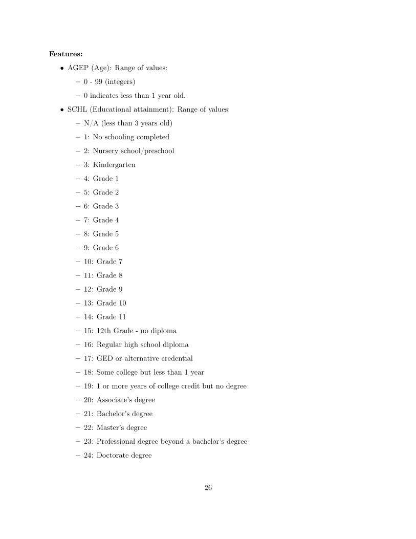
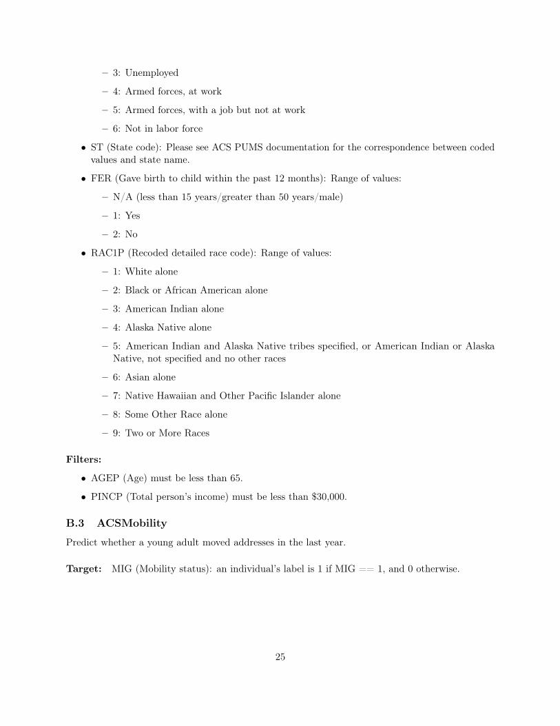
Features:








– 3: Kindergarten

– 4: Grade 1

– 5: Grade 2

– 6: Grade 3

– 7: Grade 4

– 8: Grade 5

– 9: Grade 6

– 10: Grade 7

– 11: Grade 8

– 12: Grade 9

– 13: Grade 10

– 14: Grade 11











26


– 1: Married

– 2: Widowed

– 3: Divorced

– 4: Separated



– 1: Male

– 2: Female






















27






– 1: Single

– 2: Multiple

– 3: Unclassified

– 4: Not reported



– 1: Native

– 2: Foreign born



– 1: Husband/wife






– 7: Grandchild









28




– 1: Yes

– 2: No


– 1: Yes

– 2: No



– 1: Yes

– 2: No


– 1: White alone





– 6: Asian alone




• GCL (Grandparents living with grandchildren): Range of values:

– N/A (less than 30 years/institutional GQ)

– 1: Yes

– 2: No

• COW (Class of worker): Range of values:

– N/A (not in universe)

– 1: Employee of a private for-profit company or business, or of an individual, for wages,salary, or commissions

29

– 2: Employee of a private not-for-profit, tax-exempt, or charitable organization

– 3: Local government employee (city, county, etc.)

– 4: State government employee

– 5: Federal government employee

– 6: Self-employed in own not incorporated business, professional practice, or farm

– 7: Self-employed in own incorporated business, professional practice or farm

– 8: Working without pay in family business or farm

– 9: Unemployed and last worked 5 years ago or earlier or never worked

• ESR (Employment status recode): Range of values:


– 1: Civilian employed, at work

– 2: Civilian employed, with a job but not at work

– 3: Unemployed

– 4: Armed forces, at work

– 5: Armed forces, with a job but not at work

– 6: Not in labor force

• WKHP (Usual hours worked per week past 12 months): Range of values:

– N/A (less than 16 years old / did not work during the past 12 months)

– 1 - 98 integer valued: usual hours worked

– 99: 99 or more usual hours

• JWMNP (Travel time to work): Range of values:

– N/A (not a worker or a worker that worked at home)

– integers 1 - 200 for minutes to get to work

– top-coded at 200 so values above 200 are coded as 200

• PINCP (Total person’s income): Range of values:

– integers between -19997 and 4209995 to indicate income in US dollars

– loss of $19998 or more is coded as -19998.

– income of $4209995 or more is coded as 4209995.

Filters:

• AGEP (Age) must be greater than 18 and less than 35.

30

B.4 ACSEmployment

Predict whether an adult is employed.

Target: ESR (Employment status recode): an individual’s label is 1 if ESR == 1, and 0 otherwise.

Features:








– 3: Kindergarten

– 4: Grade 1

– 5: Grade 2

– 6: Grade 3

– 7: Grade 4

– 8: Grade 5

– 9: Grade 6

– 10: Grade 7

– 11: Grade 8

– 12: Grade 9

– 13: Grade 10

– 14: Grade 11








31





– 1: Married

– 2: Widowed

– 3: Divorced

– 4: Separated



– 1: Male

– 2: Female



















32














– 1: Single

– 2: Multiple

– 3: Unclassified

– 4: Not reported



– 1: Native

– 2: Foreign born



– 1: Husband/wife






– 7: Grandchild

33












– 1: Yes

– 2: No


– 1: Yes

– 2: No



– 1: Yes

– 2: No


– 1: White alone





– 6: Asian alone




34

• GCL (Grandparents living with grandchildren): Range of values:

– N/A (less than 30 years/institutional GQ)

– 1: Yes

– 2: No

Filters:

• AGEP (Age) must be greater than 16 and less than 90.

• PWGTP (Person weight) must be greater than or equal to 1.

B.5 ACSTravelTime

Predict whether a working adult has a travel time to work of greater than 20 minutes.

Target: JWMNP (Travel time to work): an individual’s label is 1 if JWMNP > 20, and 0 otherwise.

Features:








– 3: Kindergarten

– 4: Grade 1

– 5: Grade 2

– 6: Grade 3

– 7: Grade 4

– 8: Grade 5

– 9: Grade 6

– 10: Grade 7

– 11: Grade 8

– 12: Grade 9

– 13: Grade 10

35

– 14: Grade 11












– 1: Married

– 2: Widowed

– 3: Divorced

– 4: Separated



– 1: Male

– 2: Female











36











– 1: Husband/wife






– 7: Grandchild












– 1: White alone


37




– 6: Asian alone




• PUMA (Public use microdata area code (PUMA) based on 2010 Census definition (areaswith population of 100,000 or more, use with ST for unique code)): Please see ACS PUMSdocumentation for details on the PUMA codes (which range from 100 to 70301)

• ST (State code): Please see ACS PUMS documentation for the correspondence between codedvalues and state name.







• OCCP (Occupation): Please see ACS PUMS documentation for the full list of occupationcodes

• JWTR (Means of transportation to work): Range of values:

– N/A (not a worker–not in the labor force, including persons under 16 years, unemployed,employed, with a job but not at work, Armed Forces, with a job but not at work)

– 1: Car, truck, or van

– 2: Bus or trolley bus

– 3: Streetcar or trolley car (carro publico in Puerto Rico)

– 4: Subway or elevated

– 5: Railroad

– 6: Ferryboat

– 7: Taxicab

– 8: Motorcycle

38

– 9: Bicycle

– 10: Walked;

– 11: Worked at home

– 12: Other method

• POWPUMA (Place of work PUMA based on 2010 Census definitions): Please see ACS PUMSdocumentation for details on PUMA codes

• POVPIP (Income-to-poverty ratio recode): Range of values:

– N/A

– integers 0-500

– 501 for 501 percent or more

Filters:

• AGEP (Age) must be greater than 16.

• PWGTP (Person weight) must be greater than or equal to 1.

• ESR (Employment status recode) must be equal to 1 (employed).

B.6 Dataset access and license

We provide a flexible software package to download ACS PUMS data and construct both the newprediction tasks discussed in Section 3, as well as new tasks using ACS PUMS data products.The ACS PUMS data itself is governed by the terms of service from the US Census Bureau.For more information, see https://www.census.gov/data/developers/about/terms-of-service.html Similarly, the IPUMS adult reconstruction is governed by the IPUMS terms of use. For moreinformation, see https://ipums.org/about/terms.

B.7 Table 1 experiment details

For each of the tasks listed in Table 1 (ACSIncome, ACSPublicCoverage, ACSMobility, ACSEm-ployment, ACSTravelTime), we use the 1-year 2018 US-Wide ACS PUMS data. We randomly split80% of the dataset into a training split and the remaining 20% into a test split. All features arestandardized to be zero-mean and unit-variance. Constant Predictor refers to the majority classbaseline, LogReg refers to a logistic regression baseline, and GBM refers to a gradient boosted decisiontree classifier. For each models, we use the implementation provided by Pedregosa et al. [28] withthe default hyperparameters.

C Tour of empirical observations: missing experimental details

Models and hyperparameters. All of the experiments in this section use the same uncon-strained base model: a gradient boosted decision tree (GBM). We use the implementation providedby Pedregosa et al. [28] and use exponential loss, num_estimators 5, max_depth 5, and all other

39

https://www.census.gov/data/developers/about/terms-of-service.html


https://ipums.org/about/terms

hyperparameters set to the default. These hyperparameters were chosen via a small grid search tomaximize accuracy on the ACSIncome task. We use the implementation of LFR [34] from Bellamyet al. [7] with hyperparameters k=10, Ax=0.1, Ay=1.0, Az = 2.0, maxiter=5000, and maxfun=5000.The hyperparameters are the same as those used in the UCI Adult tutorial provided by Bellamy et al.[7]. For the in-processing method (ExpGrad) from Agarwal et al. [2], we use the implementationfrom Bird et al. [9] with the default hyperparameters, and for the post-processing method, we usethe threshold adjustment method of Hardt et al. [20], which is also implemented in Bellamy et al.[7]. In Section 4, we use all of the methods to enforce demographic parity. We detail additionalexperiments enforcing equality of opportunity in Appendix D.

Datasets. Throughout this section, we use the ACSIncome task described in Section 3 andAppendix B. With the exception of the distribution shift across time experiments, we use the 20181-Year ACS PUMS data. For each state, we randomly split 80% of the dataset into a training splitand use the remaining 20% as a test split. The US-Wide dataset is constructed by combining thesetraining and testing sets over all 50 states and Puerto Rico. For the distribution shift across timeexperiments, we use the same procedure for the 2014-2017 1-Year ACS PUMS data.

Confidence intervals. To account for random variation in estimating model accuracies andviolations of demographic parity and equality of opportunity, we report each of these metrics withappropriate confidence intervals. We report and plot accuracy numbers with 95% Clopper-Pearsonintervals. We report and plot violations of demographic parity and equality of opportunity with 95%Newcombe intervals for the difference between two binomial proportions.

Compute environment. All of our experiments are run on CPUs on a cluster computer with 24Intel Xeon E7 CPUs and 300 GB of RAM.

D Additional experiments

In this section, we conduct the same set of experiments conducted in Section 4 on the 5 otherprediction tasks we introduced in Section 3. Throughout we keep the experimental details (models,hyperparameters, etc) identical to those detailed in Appendix C.

D.1 Intervention effect sizes across states

As in Section 4, we train an unconstrained gradient boosted decision tree (GBM) on each state,and we compare the accuracy and fairness criterion violation of this unconstrained model with thesame model after applying one of three common fairness intervention: pre-processing (LFR), the in-processing fair reductions methods from Agarwal et al. [2] (ExpGrad), and the simple post-processingmethod that adjusts group-based acceptance thresholds to satisfy a constraint [20]. Figure 6 showsthe result of this experiment for the ACSIncome prediction task for interventions to achieve equalityof opportunity.

In Figure 7, we conduct the same experiment for demographic parity on four other ACS data tasks:ACSPublicCoverage, ACSEmployment, ACSMobility, and ACSTravelTime, respectively.

40

0.78 0.80 0.82 0.84State accuracy

0.0

0.1

0.2

0.3

P(Y

=1

Whi

te,Y

=1)

P(Y

=1

Blac

k,Y

=1)

GBM w/ LFR

0.78 0.80 0.82 0.84State accuracy

0.0

0.1

0.2

0.3GBM w/ ExpGrad (EO)

0.78 0.80 0.82 0.84State accuracy

0.0

0.1

0.2

0.3GBM w/ Post-processing (EO)

ACSIncome


Figure 6: The effect size of fairness interventions varies by state. Each panel shows the change inaccuracy and equality of opportunity violation (EO) on the ACSIncome task after applying a fairnessintervention to an unconstrained gradient boosted decision tree (GBM). Each arrow corresponds toa different state distribution. The arrow base represents the (accuracy, EO) point corresponding tothe unconstrained GBM, and the head represents the (accuracy, EO) point obtained after applyingthe intervention. The arrow for HI in the LFR plot and ME in all three plots is entirely covered bythe start and end points.

D.2 Geographic distribution shift

In Figure 8, we plot accuracy and equality of opportunity violation with respect to race for both anunconstrained GBM and the same model after applying a post-processing adjustment to achieveequality of opportunity on a natural suite of test sets: the in-distribution (same state test set) andthe out-of-distribution test sets for the 49 other states. This is the same experiment as in Section 4,but with equality of opportunity rather than demographic parity as the metric of interest. InFigures 9, 10 11, and 12 we conduct the same experiment for demographic parity on four other ACSdata tasks: ACSPublicCoverage, ACSEmployment, ACSMobility, and ACSTravelTime, respectively.

D.3 Temporal distribution shift

In Figure 13, we plot model accuracy and equality of opportunity violation for a GBM trained onthe ACSIncome task using US-wide data from 2014 and evaluated on the test sets for the sametask drawn from years 2014-2018. This is the same experiment as conducted in Section 4; however,here we consider interventions to satisfy equality of opportunity rather than demographic parity.In Figure 14, we conduct repeat this experiment for interventions to satisfy demographic parity on4 other ACS PUMS predictions tasks: ACSPublicCoverage, ACSMobility, ACSEmployment, andACSTravelTime.

41

0.65 0.70 0.75 0.80 0.85State accuracy

0.3

0.2

0.1

0.0

0.1

P(Y

=1

Whi

te)

P(Y

=1

Blac

k) GBM w/ LFR

0.70 0.75 0.80 0.85State accuracy

0.3

0.2

0.1

0.0

0.1

GBM w/ ExpGrad (DP)

0.70 0.75 0.80 0.85State accuracy

0.30.20.10.00.1

GBM w/ Post-processing (DP)ACSPublicCoverage


0.74 0.76 0.78 0.80State accuracy

0.10

0.05

0.00

0.05

0.10

P(Y

=1

Whi

te)

P(Y

=1

Blac

k) GBM w/ LFR

0.77 0.78 0.79 0.80State accuracy

0.10

0.05

0.00

0.05


0.76 0.77 0.78 0.79 0.80State accuracy

0.10

0.05

0.00

0.05


ACSEmployment


0.700 0.725 0.750 0.775 0.800 0.825State accuracy

0.0

0.1

0.2

0.3

P(Y

=1

Whi

te)

P(Y

=1

Blac

k) GBM w/ LFR

0.74 0.76 0.78 0.80 0.82State accuracy

0.0

0.1

0.2


0.72 0.74 0.76 0.78 0.80 0.82State accuracy

0.0

0.1

0.2


ACSMobility


0.60 0.65 0.70 0.75State accuracy

0.4

0.3

0.2

0.1

0.0

P(Y

=1

Whi

te)

P(Y

=1

Blac

k) GBM w/ LFR

0.66 0.68 0.70 0.72 0.74State accuracy

0.4

0.3

0.2

0.1

0.0

GBM w/ ExpGrad (DP)

0.66 0.68 0.70 0.72 0.74State accuracy

0.4

0.3

0.2

0.1

0.0

GBM w/ Post-processing (DP)ACSTravelTime


Figure 7: The effect size of fairness interventions varies by state. Each panel shows the change inaccuracy and demographic parity violation (DP) on the ACSIncome task after applying a fairnessintervention to an unconstrained gradient boosted decision tree (GBM). Each arrow corresponds toa different state distribution. The arrow base represents the (accuracy, DP) point corresponding tothe unconstrained GBM, and the head represents the (accuracy, DP) point obtained after applyingthe intervention. When only a single point is visible, the entire arrow is covered by the point,representing an intervention that has essentially no effect.

42

0.7 0.8Accuracy

0.4

0.2

0.0

0.2

0.4

0.6

P(Y

=1

Whi

te,Y

=1)

P(Y

=1

Blac

k,Y

=1)

GBM, train on CAID (CA) evaluationOOD evaluation

0.75 0.80Accuracy

0.40.20.00.20.40.6

GBM, train on TXID (TX) evaluationOOD evaluation

0.7 0.8Accuracy

0.2

0.0

0.2

0.4

GBM, train on IN


0.70 0.75 0.80Accuracy

0.2

0.0

0.2

0.4

0.6

GBM, train on NYID (NY) evaluationOOD evaluation

ACSIncome 2018 1-Year

0.6 0.7Accuracy

0.4

0.2

0.0

0.2

0.4

0.6

P(Y

=1

Whi

te,Y

=1)

P(Y

=1

Blac

k,Y

=1) Postprocess (EO) on CA

ID (CA) evaluationOOD evaluation

0.65 0.70 0.75 0.80Accuracy

0.4

0.2

0.0

0.2

0.4

0.6Postprocess (EO) on TX


0.6 0.7 0.8Accuracy

0.50

0.25

0.00

0.25

0.50Postprocess (EO) on IN


0.70 0.75Accuracy

0.4

0.2

0.0

0.2

0.4

0.6Postprocess (EO) on NY


Figure 8: Transfer from one state to another gives unpredictable results in terms of predictiveaccuracy and fairness criteria. Top: Each panel shows an unconstrained GBM trained on a particularstate on the ACSIncome task and evaluated both in-distribution (ID) on the same state and out-of-distribution (OOD) on the 49 other states in terms of accuracy and equality of opportunity violation.Bottom: Each panel shows an GBM with post-processing to enforce equality of opportunity onthe state on which it was trained and evaluated both ID and OOD on all 50 states. Confidenceintervals are 95% Clopper-Pearson intervals for accuracy and 95% Newcombe intervals for equalityof opportunity violation.

43

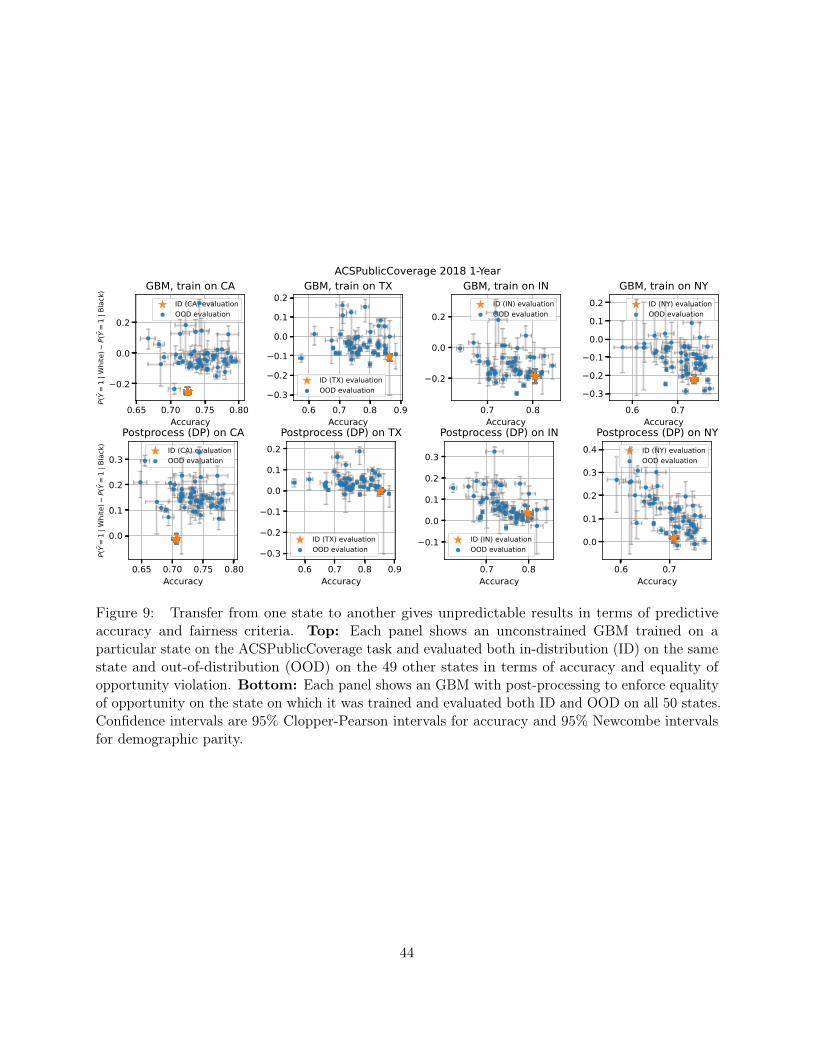
0.65 0.70 0.75 0.80Accuracy

0.2

0.0

0.2

P(Y

=1

Whi

te)

P(Y

=1

Blac

k)


0.6 0.7 0.8 0.9Accuracy

0.3

0.2

0.1

0.0

0.1

0.2GBM, train on TX


0.7 0.8Accuracy

0.2

0.0

0.2

GBM, train on INID (IN) evaluationOOD evaluation

0.6 0.7Accuracy

0.30.20.10.00.10.2


ACSPublicCoverage 2018 1-Year

0.65 0.70 0.75 0.80Accuracy

0.0

0.1

0.2

0.3

P(Y

=1

Whi

te)

P(Y

=1

Blac

k)

Postprocess (DP) on CAID (CA) evaluationOOD evaluation

0.6 0.7 0.8 0.9Accuracy

0.3

0.2

0.1

0.0

0.1

0.2Postprocess (DP) on TX


0.7 0.8Accuracy

0.1

0.0

0.1

0.2

0.3

Postprocess (DP) on IN


0.6 0.7Accuracy

0.0

0.1

0.2

0.3

0.4Postprocess (DP) on NY


Figure 9: Transfer from one state to another gives unpredictable results in terms of predictiveaccuracy and fairness criteria. Top: Each panel shows an unconstrained GBM trained on aparticular state on the ACSPublicCoverage task and evaluated both in-distribution (ID) on the samestate and out-of-distribution (OOD) on the 49 other states in terms of accuracy and equality ofopportunity violation. Bottom: Each panel shows an GBM with post-processing to enforce equalityof opportunity on the state on which it was trained and evaluated both ID and OOD on all 50 states.Confidence intervals are 95% Clopper-Pearson intervals for accuracy and 95% Newcombe intervalsfor demographic parity.

44

0.70 0.75Accuracy

0.2

0.0

0.2

P(Y

=1

Whi

te)

P(Y

=1

Blac

k)

GBM, train on CA


0.70 0.75 0.80Accuracy

0.1

0.0

0.1

0.2

0.3GBM, train on TX


0.70 0.75 0.80Accuracy

0.1

0.0

0.1

0.2

0.3


0.70 0.75 0.80Accuracy

0.2

0.1

0.0

0.1

0.2


ACSEmployment 2018 1-Year

0.70 0.75Accuracy

0.2

0.0

0.2

P(Y

=1

Whi

te)

P(Y

=1

Blac

k)


0.70 0.75 0.80Accuracy

0.2

0.1

0.0

0.1

0.2

Postprocess (DP) on TX


0.70 0.75 0.80Accuracy

0.2

0.1

0.0

0.1

0.2

0.3Postprocess (DP) on IN


0.70 0.75Accuracy

0.3

0.2

0.1

0.0

0.1

0.2


Figure 10: Transfer from one state to another gives unpredictable results in terms of predictiveaccuracy and fairness criteria. Top: Each panel shows an unconstrained GBM trained on aparticular state on the ACSEmployment task and evaluated both in-distribution (ID) on the samestate and out-of-distribution (OOD) on the 49 other states in terms of accuracy and equality ofopportunity violation. Bottom: Each panel shows an GBM with post-processing to enforce equalityof opportunity on the state on which it was trained and evaluated both ID and OOD on all 50 states.Confidence intervals are 95% Clopper-Pearson intervals for accuracy and 95% Newcombe intervalsfor demographic parity.

45

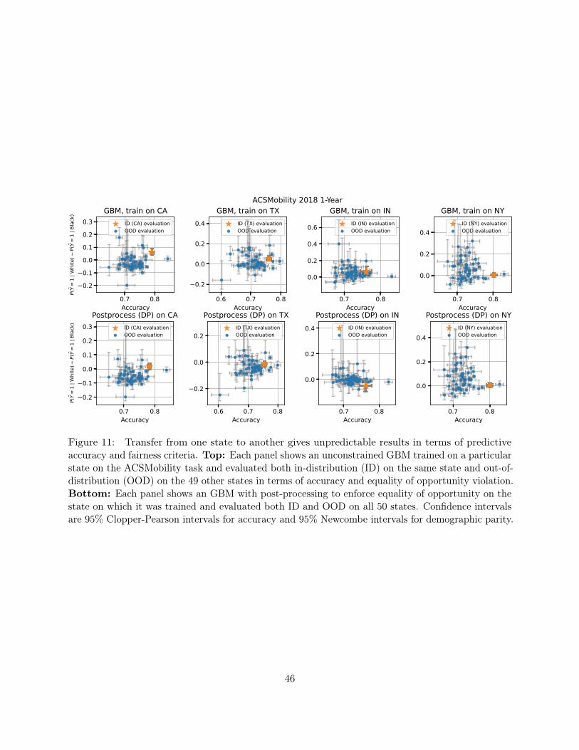
0.7 0.8Accuracy

0.20.10.00.10.20.3

P(Y

=1

Whi

te)

P(Y

=1

Blac

k)


0.6 0.7 0.8Accuracy

0.2

0.0

0.2

0.4GBM, train on TX


0.7 0.8Accuracy

0.0

0.2

0.4

0.6


0.7 0.8Accuracy

0.0

0.2

0.4


ACSMobility 2018 1-Year

0.7 0.8Accuracy

0.2

0.1

0.0

0.1

0.2

0.3

P(Y

=1

Whi

te)

P(Y

=1

Blac

k)


0.6 0.7 0.8Accuracy

0.2

0.0

0.2

Postprocess (DP) on TXID (TX) evaluationOOD evaluation

0.7 0.8Accuracy

0.0

0.2

0.4

Postprocess (DP) on INID (IN) evaluationOOD evaluation

0.7 0.8Accuracy

0.0

0.2

0.4


Figure 11: Transfer from one state to another gives unpredictable results in terms of predictiveaccuracy and fairness criteria. Top: Each panel shows an unconstrained GBM trained on a particularstate on the ACSMobility task and evaluated both in-distribution (ID) on the same state and out-of-distribution (OOD) on the 49 other states in terms of accuracy and equality of opportunity violation.Bottom: Each panel shows an GBM with post-processing to enforce equality of opportunity on thestate on which it was trained and evaluated both ID and OOD on all 50 states. Confidence intervalsare 95% Clopper-Pearson intervals for accuracy and 95% Newcombe intervals for demographic parity.

46

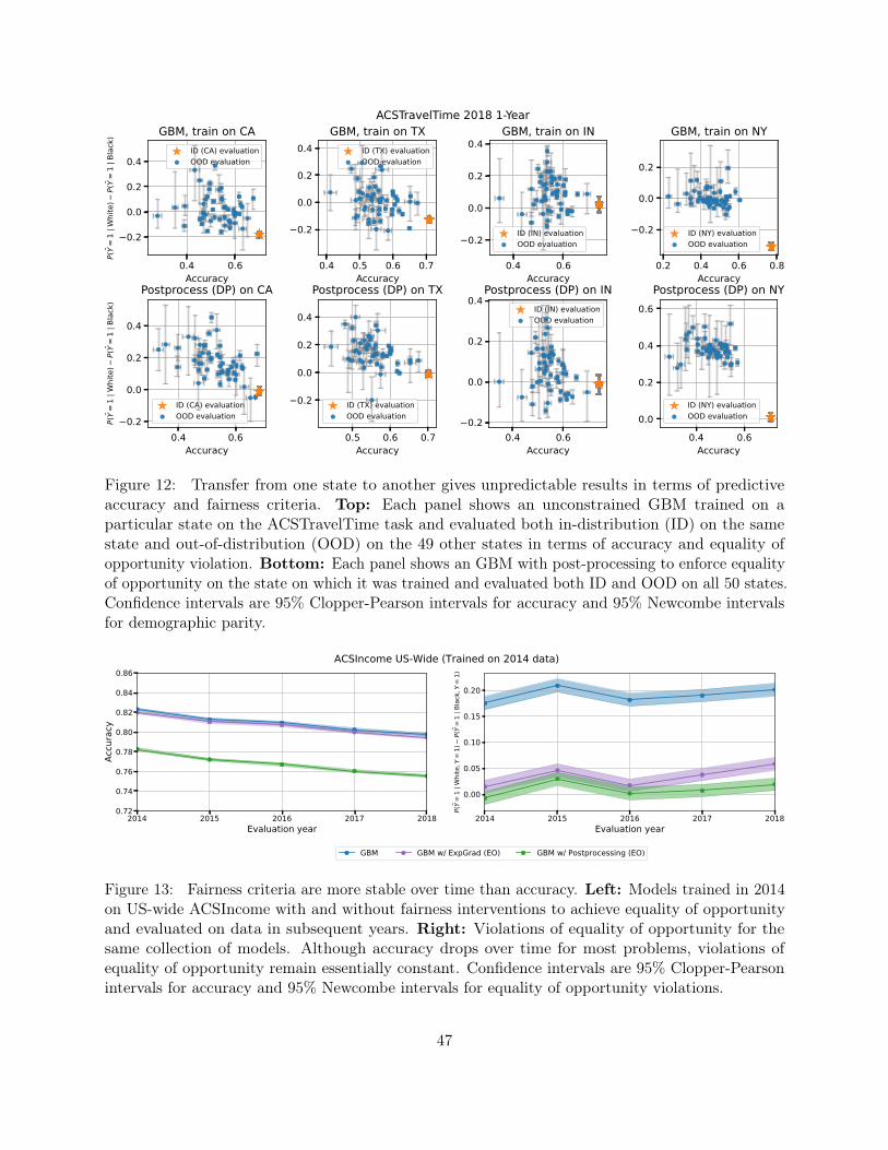
0.4 0.6Accuracy

0.2

0.0

0.2

0.4

P(Y

=1

Whi

te)

P(Y

=1

Blac

k)


0.4 0.5 0.6 0.7Accuracy

0.2

0.0

0.2

0.4GBM, train on TX


0.4 0.6Accuracy

0.2

0.0

0.2

0.4GBM, train on IN


0.2 0.4 0.6 0.8Accuracy

0.2

0.0

0.2

GBM, train on NY


ACSTravelTime 2018 1-Year

0.4 0.6Accuracy

0.2

0.0

0.2

0.4

P(Y

=1

Whi

te)

P(Y

=1

Blac

k)

Postprocess (DP) on CA


0.5 0.6 0.7Accuracy

0.2

0.0

0.2

0.4

Postprocess (DP) on TX


0.4 0.6Accuracy

0.2

0.0

0.2

0.4Postprocess (DP) on IN


0.4 0.6Accuracy

0.0

0.2

0.4

0.6Postprocess (DP) on NY


Figure 12: Transfer from one state to another gives unpredictable results in terms of predictiveaccuracy and fairness criteria. Top: Each panel shows an unconstrained GBM trained on aparticular state on the ACSTravelTime task and evaluated both in-distribution (ID) on the samestate and out-of-distribution (OOD) on the 49 other states in terms of accuracy and equality ofopportunity violation. Bottom: Each panel shows an GBM with post-processing to enforce equalityof opportunity on the state on which it was trained and evaluated both ID and OOD on all 50 states.Confidence intervals are 95% Clopper-Pearson intervals for accuracy and 95% Newcombe intervalsfor demographic parity.

2014 2015 2016 2017 2018Evaluation year

0.72

0.74

0.76

0.78

0.80

0.82

0.84

0.86

Accu

racy

2014 2015 2016 2017 2018Evaluation year

0.00

0.05

0.10

0.15

0.20

P(Y

=1

Whi

te,Y

=1)

P(Y

=1

Blac

k,Y

=1)

ACSIncome US-Wide (Trained on 2014 data)

GBM GBM w/ ExpGrad (EO) GBM w/ Postprocessing (EO)

Figure 13: Fairness criteria are more stable over time than accuracy. Left: Models trained in 2014on US-wide ACSIncome with and without fairness interventions to achieve equality of opportunityand evaluated on data in subsequent years. Right: Violations of equality of opportunity for thesame collection of models. Although accuracy drops over time for most problems, violations ofequality of opportunity remain essentially constant. Confidence intervals are 95% Clopper-Pearsonintervals for accuracy and 95% Newcombe intervals for equality of opportunity violations.

47

2014 2015 2016 2017 2018Evaluation year

0.72

0.74

0.76

0.78

0.80

0.82

0.84

Accu

racy

2014 2015 2016 2017 2018Evaluation year

0.14

0.12

0.10

0.08

0.06

0.04

0.02

0.00

P(Y

=1

Whi

te)

P(Y

=1

Blac

k)

PUMSPublicCoverage US-Wide (Trained on 2014 data)

GBM GBM w/ Postprocessing (DP) GBM w/ LFR

2014 2015 2016 2017 2018Evaluation year

0.72

0.74

0.76

0.78

0.80

0.82

0.84

Accu

racy

2014 2015 2016 2017 2018Evaluation year

0.00

0.02

0.04

0.06

0.08

P(Y

=1

Whi

te)

P(Y

=1

Blac

k)

PUMSEmployment US-Wide (Trained on 2014 data)


2014 2015 2016 2017 2018Evaluation year

0.70

0.72

0.74

0.76

0.78

0.80

Accu

racy

2014 2015 2016 2017 2018Evaluation year

0.00

0.02

0.04

0.06

0.08

0.10

P(Y

=1

Whi

te)

P(Y

=1

Blac

k)

PUMSMobility US-Wide (Trained on 2014 data)


2014 2015 2016 2017 2018Evaluation year

0.60

0.62

0.64

0.66

0.68

0.70

Accu

racy

2014 2015 2016 2017 2018Evaluation year

0.12

0.10

0.08

0.06

0.04

0.02

0.00

0.02

P(Y

=1

Whi

te)

P(Y

=1

Blac

k)

PUMSTravelTime US-Wide (Trained on 2014 data)


Figure 14: Fairness criteria are more stable over time than accuracy. Left: Models trained in2014 on US-wide ACS data with and without fairness interventions to achieve demographic parityand evaluated on data in subsequent years. Right: Violations of demographic parity for thesame collection of models. Although accuracy drops over time for most problems, violations ofdemographic parity remain essentially constant. Confidence intervals are 95% Clopper-Pearsonintervals for accuracy and 95% Newcombe intervals for demographic parity.

48

E Datasheet

This datasheet covers both the prediction tasks we introduce and the underlying US Census datasources. However, due to the extensive documentation available about the US Census data we oftenpoint to relevant available resources rather than recreating them here. For the most up-to-date versionof this datasheet, please refer to https://github.com/zykls/folktables/blob/main/datasheet.md.

E.1 Motivation

• For what purpose was the dataset created? Was there a specific task in mind? Was therea specific gap that needed to be filled? Please provide a description.

The motivation for creating prediction tasks on top of US Census data was to extend the datasetecosystem available for algorithmic fairness research as outlined in this paper.

• Who created the dataset (e.g., which team, research group) and on behalf of whichentity (e.g., company, institution, organization)?

The new prediction tasks were created from available US Census data sources by Frances Ding,Moritz Hardt, John Miller, and Ludwig Schmidt.

• Who funded the creation of the dataset? If there is an associated grant, please provide thename of the grantor and the grant name and number.

Frances Ding, Moritz Hardt, and John Miller were employed by the University of California forthe duration of this research project, funded by grants administered through the University ofCalifornia. Ludwig Schmidt was employed by Toyota Research throughout this research project.

• Any other comments?

No.

E.2 Composition

• What do the instances that comprise the dataset represent (e.g., documents, photos,people, countries)? Are there multiple types of instances (e.g., movies, users, and ratings;people and interactions between them; nodes and edges)? Please provide a description.

Each instance in our IPUMS Adult reconstruction represents an individual. Similarly, our datasetsderived from ACS contains instances representing individuals. The ACS data our datasets arederived from also contain household-level information and the relationship between householdsand individuals.

• How many instances are there in total (of each type, if appropriate)?

Our IPUMS Adult reconstruction contains 49,531 rows (see Section 2.1). Table 1 contains thesizes of our datasets derived from ACS.

• Does the dataset contain all possible instances or is it a sample (not necessarilyrandom) of instances from a larger set? If the dataset is a sample, then what is the largerset? Is the sample representative of the larger set (e.g., geographic coverage)? If so, please describe

49

https://github.com/zykls/folktables/blob/main/datasheet.md

https://github.com/zykls/folktables/blob/main/datasheet.md

how this representativeness was validated/verified. If it is not representative of the larger set,please describe why not (e.g., to cover a more diverse range of instances, because instances werewithheld or unavailable)

Both IPUMS Adult and our ACS datasets are samples of the US population. Please see Sections2.1 & 3 and the corresponding documentation provided by the US Census Bureau. Note that theper-instance weights have to be taken into account if the sample is meant to represent the USpopulation.

• What data does each instance consist of? “Raw” data (e.g., unprocessed text or images) orfeatures? In either case, please provide a description.

Each instance consists of features. IPUMS Adult uses the same features as the original UCI Adultdataset. Appendix B describes each feature in our new datasets derived from ACS.

• Is there a label or target associated with each instance? If so, please provide a description.

Similar to UCI Adult, our IPUMS Adult reconstruction uses the income as label (where thecontinuous values as opposed to only the binarized values are now available). Appendix B describesthe labels in our new datasets derived from ACS.

• Is any information missing from individual instances? If so, please provide a description,explaining why this information is missing (e.g., because it was unavailable). This does not includeintentionally removed information, but might include, e.g., redacted text.

Some features (e.g., the country of origin in IPUMS Adult) contain missing values. We again referto the respective documentation from the US Census Bureau for details.

• Are relationships between individual instances made explicit (e.g., users’ movie rat-ings, social network links)? If so, please describe how these relationships are made explicit.

Our versions of the datasets contain no relationships between individuals. The original datasources from the US Census contain relationships between individuals and households.

• Are there recommended data splits (e.g., training, development/validation, testing)?If so, please provide a description of these splits, explaining the rationale behind them.

For IPUMS Adult, it is possible to follow the same train / test split as the original UCI Adult. Ingeneral, we recommend k-fold cross-validation for all of our datasets.

• Are there any errors, sources of noise, or redundancies in the dataset? If so, pleaseprovide a description.

Our IPUMS Adult reconstruction contains slightly more rows than the original UCI Adult, seeSection 2.1. Beyond IPUMS Adult, we refer to the documentation of CPS and ACS provided bythe US Census Bureau.

• Is the dataset self-contained, or does it link to or otherwise rely on external resources(e.g., websites, tweets, other datasets)? If it links to or relies on external resources, a) arethere guarantees that they will exist, and remain constant, over time; b) are there official archivalversions of the complete dataset (i.e., including the external resources as they existed at the timethe dataset was created); c) are there any restrictions (e.g., licenses, fees) associated with any

50

of the external resources that might apply to a future user? Please provide descriptions of allexternal resources and any restrictions associated with them, as well as links or other access points,as appropriate.

Due to restrictions on the re-distribution of the original IPUMS and ACS data sources, we do notprovide our datasets as standalone data files. Instead, we provide scripts to generate our datasetsfrom the respective sources.

Both the US Census Bureau and IPUMS aim to provide stable long-term access to their data.Hence we consider these data sources to be reliable. We refer to the IPUMS website and thewebsite of the US Census Bureau for specific usage restrictions. Neither data source has feesassociated with it.

• Does the dataset contain data that might be considered confidential (e.g., data that isprotected by legal privilege or by doctor patient confidentiality, data that includes thecontent of individuals’ non-public communications)? If so, please provide a description.

Our datasets are subsets of datasets released publicly by the US Census Bureau.

• Does the dataset contain data that, if viewed directly, might be offensive, insulting,threatening, or might otherwise cause anxiety? If so, please describe why.

No.

• Does the dataset relate to people? If not, you may skip the remaining questions in thissection.

Yes, each instance in our datasets corresponds to a person.

• Does the dataset identify any subpopulations (e.g., by age, gender)? If so, pleasedescribe how these subpopulations are identified and provide a description of their respectivedistributions within the dataset.

Our datasets identify subpopulations since each individual has features such as age, gender, orrace. Please see the main text of our paper for experiments exploring the respective distributions.

• Is it possible to identify individuals (i.e., one or more natural persons), either directlyor indirectly (i.e., in combination with other data) from the dataset? If so, pleasedescribe how.

To the best of our knowledge, it is not possible to identify individuals directly from our datasets.However, the possibility of reconstruction attacks combining data from the US Cenus Bureau(such as CPS and ACS) and other data sources are a concern and actively investigated by theresearch community.

• Does the dataset contain data that might be considered sensitive in any way (e.g.,data that reveals racial or ethnic origins, sexual orientations, religious beliefs, politi-cal opinions or union memberships, or locations; financial or health data; biometricor genetic data; forms of government identification, such as social security numbers;criminal history)? If so, please provide a description.

51

Our datasets contain features such as race, age, or gender that are often considered sensitive. Thisis by design since we assembled our datasets to test algorithmic fairness interventions.


No.

E.3 Collection process

• How was the data associated with each instance acquired? Was the data directly observ-able (e.g., raw text, movie ratings), reported by subjects (e.g., survey responses), or indirectlyinferred/derived from other data (e.g., part-of-speech tags, model-based guesses for age or lan-guage)? If data was reported by subjects or indirectly inferred/derived from other data, was thedata validated/verified? If so, please describe how.

The data was reported by subjects as part of the ACS and CPS surveys. The respective docu-mentation provided by the US Census Bureau contains further information, see https://www.census.gov/programs-surveys/acs/methodology/design-and-methodology.html and https://www.census.gov/programs-surveys/cps/technical-documentation/methodology.html.

• What mechanisms or procedures were used to collect the data (e.g., hardware appa-ratus or sensor, manual human curation, software program, software API)? How werethese mechanisms or procedures validated?

The ACS relies on a combination of internet, mail, telephone, and in-person interviews. CPS usesin-person and telephone interviews. Please see the aforementioned documentation from the USCensus Bureau for detailed information.

• If the dataset is a sample from a larger set, what was the sampling strategy (e.g.,deterministic, probabilistic with specific sampling probabilities)?

For the ACS, the US Census Bureau sampled housing units uniformly for each county. See Chapter4 in the ACS documentation (https://www2.census.gov/programs-surveys/acs/methodology/design_and_methodology/acs_design_methodology_report_2014.pdf) for details.

CPS is also sampled by housing unit from certain sampling areas, see Chapters 3 and 4 inhttps://www.census.gov/prod/2006pubs/tp-66.pdf.

• Who was involved in the data collection process (e.g., students, crowdworkers, con-tractors) and how were they compensated (e.g., how much were crowdworkers paid)?

The US Census Bureau employs interviewers for conducting surveys. According to online jobinformation platforms such as indeed.com, an interviewer earns about $15 per hour.

• Over what timeframe was the data collected? Does this timeframe match the creationtimeframe of the data associated with the instances (e.g., recent crawl of old news articles)? Ifnot, please describe the timeframe in which the data associated with the instances was created.

Both CPS and ACS collect data annually. Our IPUMS Adult reconstruction contains data fromthe 1994 CPS ASEC. Our new tasks derived from ACS can be instantiated for various surveyyears.

52

https://www.census.gov/programs-surveys/acs/methodology/design-and-methodology.html

https://www.census.gov/programs-surveys/acs/methodology/design-and-methodology.html

https://www.census.gov/programs-surveys/cps/technical-documentation/methodology.html


https://www2.census.gov/programs-surveys/acs/methodology/design_and_methodology/acs_design_methodology_report_2014.pdf

https://www2.census.gov/programs-surveys/acs/methodology/design_and_methodology/acs_design_methodology_report_2014.pdf

https://www.census.gov/prod/2006pubs/tp-66.pdf

indeed.com

• Were any ethical review processes conducted (e.g., by an institutional review board)?If so, please provide a description of these review processes, including the outcomes, as well as alink or other access point to any supporting documentation.

Both ACS and CPS are regularly reviewed by the US Census Bureau. As a government agency,the US Census Bureau is also subject to government oversight mechanisms.

• Does the dataset relate to people? If not, you may skip the remainder of the questionsin this section.

Yes.

• Did you collect the data from the individuals in question directly, or obtain it viathird parties or other sources (e.g., websites)?

Data collection was performed by the US Census Bureau. We obtained the data from publiclyavailable US Census repositories.

• Were the individuals in question notified about the data collection? If so, please describe(or show with screenshots or other information) how notice was provided, and provide a link orother access point to, or otherwise reproduce, the exact language of the notification itself.

Yes. A sample ACS form is available online: https://www.census.gov/programs-surveys/acs/about/forms-and-instructions/2021-form.html

Information about the CPS collection methodology is available here: https://www.census.gov/programs-surveys/cps/technical-documentation/methodology.html

• Did the individuals in question consent to the collection and use of their data? If so,please describe (or show with screenshots or other information) how consent was requested andprovided, and provide a link or other access point to, or otherwise reproduce, the exact languageto which the individuals consented.

Participation in the US Census American Community Survey is mandatory. Participation in the USCorrent Population Survey is voluntary and consent is obtained at the beginning of the interview:https://www2.census.gov/programs-surveys/cps/methodology/CPS-Tech-Paper-77.pdf

• If consent was obtained, were the consenting individuals provided with a mechanismto revoke their consent in the future or for certain uses? If so, please provide a description,as well as a link or other access point to the mechanism (if appropriate).

We are not aware that the Census Bureau would provide such a mechanism.

• Has an analysis of the potential impact of the dataset and its use on data subjects(e.g., a data protection impact analysis) been conducted? If so, please provide a descriptionof this analysis, including the outcomes, as well as a link or other access point to any supportingdocumentation.

The US Census Bureau assesses privacy risks and invests in statistical disclosure control. Seehttps://www.census.gov/topics/research/disclosure-avoidance.html. Our derived predic-tion tasks do not increase privacy risks.


53

https://www.census.gov/programs-surveys/acs/about/forms-and-instructions/2021-form.html

https://www.census.gov/programs-surveys/acs/about/forms-and-instructions/2021-form.html



https://www2.census.gov/programs-surveys/cps/methodology/CPS-Tech-Paper-77.pdf

https://www.census.gov/topics/research/disclosure-avoidance.html

No.

E.4 Preprocessing / cleaning / labeling

• Was any preprocessing/cleaning/labeling of the data done (e.g., discretization orbucketing, tokenization, part-of-speech tagging, SIFT feature extraction, removal ofinstances, processing of missing values)? If so, please provide a description. If not, you mayskip the remainder of the questions in this section.

We used two US Census data products – we reconstructed UCI Adult from the Annual Socialand Economic Supplement (ASEC) of the Current Population Survey (CPS), and we constructednew prediction tasks from the American Community Survey (ACS) Public Use Microdata Sample(PUMS). Before releasing CPS data publicly, the Census Bureau top-codes certain variables andconducts imputation of certain missing values, as documented here: https://www.census.gov/programs-surveys/cps/technical-documentation/methodology.html. In our IPUMS Adultreconstruction, we include a subset of the variables available from the CPS data and do not altertheir values.

The ACS data release similarly top-codes certain variables and conducts imputation of certain miss-ing values, as documented here: https://www.census.gov/programs-surveys/acs/microdata/documentation.html. For the new prediction tasks that we define, we further process the ACSdata as documented at the folktables GitHub page, https://github.com/zykls/folktables. Inmost cases, this involves mapping missing values (NaNs) to −1. We release code so that newprediction tasks may be defined on the ACS data, with potentially different preprocessing. Eachprediction task also defines a binary label by discretizing the target variable into two classes; thiscan be easily changed to define a new labeling in a new prediction task.

• Was the “raw” data saved in addition to the preprocessed/cleaned/labeled data (e.g.,to support unanticipated future uses)? If so, please provide a link or other access point tothe “raw” data.

Yes, our package provides access to the data as released by the U.S. Census Bureau. The “raw”survey answers collected by the Census Bureau are not available for public release due to privacyconsiderations.

• Is the software used to preprocess/clean/label the instances available? If so, pleaseprovide a link or other access point.

The software to is available at the folktables GitHub page, https://github.com/zykls/folktables.


No.

E.5 Uses

• Has the dataset been used for any tasks already? If so, please provide a description.

In this paper we create five new prediction tasks from the ACS PUMS data:

1. ACSIncome: Predict whether US working adults’ yearly income is above $50,000.

54



https://www.census.gov/programs-surveys/acs/microdata/documentation.html

https://www.census.gov/programs-surveys/acs/microdata/documentation.html



2. ACSPublicCoverage: Predict whether a low-income individual, not eligible for Medicare, hascoverage from public health insurance.

3. ACSMobility: Predict whether a young adult moved addresses in the last year.

4. ACSEmployment: Predict whether a US adult is employed.

5. ACSTravelTime: Predict whether a working adult has a travel time to work of greater than20 minutes.

Further details about these tasks can be found at the folktables GitHub page, https://github.com/zykls/folktables, and in Appendix B.

• Is there a repository that links to any or all papers or systems that use the dataset?If so, please provide a link or other access point.

At the folktables GitHub page, https://github.com/zykls/folktables, any public forks to thepackage are visible, and papers or systems that use the datasets should cite the paper linked atthat Github page.

• What (other) tasks could the dataset be used for?

New prediction tasks may be defined on the ACS PUMS data that use different subsets ofvariables as features and/or different target variables. Different prediction tasks may have differentproperties such as Bayes error rate, or the base rate disparities between subgroups, that can helpto benchmark machine learning models in diverse settings.

• Is there anything about the composition of the dataset or the way it was collectedand preprocessed/cleaned/labeled that might impact future uses? For example, is thereanything that a future user might need to know to avoid uses that could result in unfair treatmentof individuals or groups (e.g., stereotyping, quality of service issues) or other undesirable harms(e.g., financial harms, legal risks) If so, please provide a description. Is there anything a futureuser could do to mitigate these undesirable harms?

Both the CPS and ACS are collected through surveys of a subset of the US population, andin their documentation, they acknowledge that statistical trends in individual states may benoisy compared to those found by analyzing US data as a whole, due to small sample sizes incertain states. In particular, there may be very few individuals with particular characteristics(e.g. ethnicity) in certain states, and generalizing conclusions from these few individuals maybe highly inaccurate. Further, benchmarking fair machine learning algorithms on datasets withfew representatives of certain subgroups may provide the illusion of “checking a box” for fairness,without substantive merit.

• Are there tasks for which the dataset should not be used? If so, please provide adescription.

This dataset contains personal information, and users should not attempt to re-identify individualsin it. Further, these datasets are meant primarily to aid in benchmarking machine learningalgorithms; Census data is often crucial for substantive, domain-specific work by social scientists,but our dataset contributions are not in this direction. Substantive investigations into inequality,

55




demographic shifts, and other important questions should not be based purely on the datasets weprovide.


No.

E.6 Distribution

• Will the dataset be distributed to third parties outside of the entity (e.g., company,institution, organization) on behalf of which the dataset was created? If so, pleaseprovide a description.

The dataset will be available for public download on the folktables GitHub page, https://github.com/zykls/folktables.

• How will the dataset will be distributed (e.g., tarball on website, API, GitHub)?Does the dataset have a digital object identifier (DOI)?

The dataset will be be distributed via GitHub, see https://github.com/zykls/folktables. Thedataset does not have a DOI.

• When will the dataset be distributed?

The dataset will be released on August 1, 2021 and available thereafter for download and publicuse.

• Will the dataset be distributed under a copyright or other intellectual property (IP)license, and/or under applicable terms of use (ToU)? If so, please describe this licenseand/or ToU, and provide a link or other access point to, or otherwise reproduce, any relevantlicensing terms or ToU, as well as any fees associated with these restrictions.

The folktables package and data loading code will be available under the MIT license. Thefolktables data itself is based on data from the American Community Survey (ACS) Public UseMicrodata Sample (PUMS) files managed by the US Census Bureau, and it is governed by theterms of use provided by the Census Bureau. For more information, see https://www.census.gov/data/developers/about/terms-of-service.html

Similarly, the IPUMS adult reconstruction is governed by the IPUMS terms of use. For moreinformation, see https://ipums.org/about/terms.

• Have any third parties imposed IP-based or other restrictions on the data associatedwith the instances? If so, please describe these restrictions, and provide a link or other accesspoint to, or otherwise reproduce, any relevant licensing terms, as well as any fees associated withthese restrictions.

The folktables data and the adult reconstruction data are governed by third-party terms ofuse provided by the US Census Bureau and IPUMS, respectively. See https://www.census.gov/data/developers/about/terms-of-service.html and https://ipums.org/about/termsfor complete details. The IPUMS Adult Reconstruction is a subsample of the IPUMS CPS dataavailable from cps.ipums.org These data are intended for replication purposes only. Individuals

56










cps.ipums.org

analyzing the data for other purposes must submit a separate data extract request directly viaIPUMS CPS. Individuals should contact [email protected] for redistribution requests.

• Do any export controls or other regulatory restrictions apply to the dataset or toindividual instances? If so, please describe these restrictions, and provide a link or other accesspoint to, or otherwise reproduce, any supporting documentation.

To our knowledge, no export controls or regulatory restrictions apply to the dataset.


No.

E.7 Maintenance

• Who is supporting/hosting/maintaining the dataset?

The dataset will be hosted on GitHub, and supported and maintained by the folktables team. Asof June 2021, this team consists of Frances Ding, Moritz Hardt, John Miller, and Ludwig Schmidt.

• How can the owner/curator/manager of the dataset be contacted (e.g., email ad-dress)?

Please send issues and requests to [email protected].

• Is there an erratum? If so, please provide a link or other access point.

An erratum will be hosted on the dataset website, https://github.com/zykls/folktables.

• Will the dataset be updated (e.g., to correct labeling errors, add new instances, deleteinstances)? If so, please describe how often, by whom, and how updates will be communicatedto users (e.g., mailing list, GitHub)?

The dataset will be updated as required to address errors and refine the prediction problemsbased on feedback from the community. The package maintainers will update the dataset andcommunicate these updates on GitHub.

• If the dataset relates to people, are there applicable limits on the retention of thedata associated with the instances (e.g., were individuals in question told that theirdata would be retained for a fixed period of time and then deleted)? If so, pleasedescribe these limits and explain how they will be enforced.

The data used in folktables is based on data from the American Community Survey (ACS) PublicUse Microdata Sample (PUMS) files managed by the US Census Bureau. The data inherits andwill respect the corresponding retention policies of the ACS. Please see https://www.census.gov/programs-surveys/acs/about.html for more details. For the Adult reconstruction dataset, thedata is based on Current Population Survey (CPS) released by IPUMS and thus inherits and willrespect the corresponding retention policies for the CPS. Please see https://cps.ipums.org/cps/for more details.

• Will older versions of the dataset continue to be supported/hosted/maintained? Ifso, please describe how. If not, please describe how its obsolescence will be communicated to users.

57

[email protected]

[email protected]


https://www.census.gov/programs-surveys/acs/about.html

https://www.census.gov/programs-surveys/acs/about.html

https://cps.ipums.org/cps/

Older versions of the datasets in folktables will be clearly indicated, supported, and maintainedon the GitHub website. Each new version of the dataset will be tagged with version metadataand an associated GitHub release.

• If others want to extend/augment/build on/contribute to the dataset, is there amechanism for them to do so? If so, please provide a description. Will these contributionsbe validated/verified? If so, please describe how. If not, why not? Is there a process forcommunicating/distributing these contributions to other users? If so, please provide a description.

Users wishing to contribute to folktables datasets are encouraged to do so by submitting a pullrequest on the website https://github.com/zykls/folktables/pulls. The contributions willbe reviewed by the maintainers. These contributions will be reflected in new version of the datasetand broadcasted as part of each Github release.


No.

58

https://github.com/zykls/folktables/pulls

Documents

Retiring Adult: New Datasets for Fair Machine Learning