Results of Operations Volume 03 – Depreciation Study of Operations Volume 03 – Depreciation Study Before the Public Utilities Commission of the State of California Rosemead, California

Application No.: A.16-09- Exhibit No.: SCE-09, Vol. 03 Witnesses: P. Joseph

A. Varvis R. White

(U 338-E)

Results of Operations Volume 03 – Depreciation Study

Before the

Public Utilities Commission of the State of California

Rosemead, California

September 1, 2016

SCE-09: Results of Operation Volume 03 - Depreciation Study

Table Of Contents Section Page Witness

-i-

I. INTRODUCTION .............................................................................................1 A. Varvis

A. Organization of Testimony ....................................................................2

B. SCE’s Depreciation Proposals ...............................................................3

C. Application of Gradualism Principle to SCE’s Proposal .......................5

D. Summary Tables ....................................................................................8

II. COMMISSION DIRECTIVES FROM SCE’S 2015 GRC DECISION .......................................................................................................11

A. The Four Directives Established in the 2015 GRC Decision ..............11

B. SCE’s Approach to Addressing the Compliance Directives from the 2015 GRC Decision ..............................................................12

1. The First Directive – Per Unit Net Salvage Analysis ..............14

a) Traditional Approaches to Analyzing Historical and Future Net Salvage ...............................15

b) Comparing the Differences Between Calculating Net Salvage Ratios Using a Traditional Analysis Versus Per-Unit Analysis........................................................................16

2. The Second Directive – Retirement Mix .................................18

3. The Third Directive – The Age of Retirements and Integration of Salvage and Life Analyses ................................19

4. The Fourth Directive – Process for Assigning Costs ...............20

C. Process for Assigning Costs to Installation and Removal (The Fourth Directive) .........................................................................20

1. Project-Specific Estimating (Bulk-Power Transmission, Substation, and Generation/Other) ...................21

a) Bulk Power Transmission and Substation (Accounts 350-359) .....................................................21


Table Of Contents (Continued) Section Page Witness

-ii-

b) Generation and Other (Accounts 301-348, and 390-398) ................................................................21

2. Design Manager (DM) Estimating (Distribution/Sub-Transmission Assets) ..................................22

a) Building a Project Estimate in DM Using Compatible Units (CUs) ..............................................22

b) Cost Allocation in PowerPlan ......................................23

3. Substantiating SCE’s Standard Rates Table Allocation Factors ....................................................................25

a) 2004 Study ...................................................................26

b) 2006 Study ...................................................................27

c) 2016 Study ...................................................................28

(1) Background of Development of Compatible Units (CUs). .................................28

(2) 2009-2010 Labor Study ...................................28 P. Joseph

(3) 2016 Comparison of Standard Rates Table and CUs ..................................................30 A. Varvis

D. SCE’s Experience with Increasingly Negative Net Salvage Rates .....................................................................................................30

1. The Average Age of Retirements is Increasing .......................31

a) Age and Inflation Impacts on Recorded Net Salvage Ratios ..............................................................31

b) SCE’s Aging Retirements ............................................32

2. Total Cost Increases Affect Cost of Removal ..........................33

3. SCE’s Per-Unit Analysis is Indifferent to the Realized Net Salvage Ratios ....................................................34

III. DEPRECIATION STUDY ..............................................................................36



-iii-

A. T&D - Average Service Life and Net Salvage Proposals ....................37 R. White

1. Development of Depreciation Rates ........................................37

2. 2016 Service–Life Study..........................................................39

3. 2016 Net Salvage Study ...........................................................43

a) Directive No. 1 .............................................................45

b) Directive No. 2 .............................................................49

c) Directive No. 3 .............................................................49

d) Directive No. 4 .............................................................50

B. Generation and G&I - Average Service Life and Net Salvage Proposals ................................................................................51 A. Varvis

1. Purpose and Scope ...................................................................51

2. Generation-Related Property ...................................................51

a) Average Service Lives for Generation Assets ...........................................................................51

(1) Palo Verde Nuclear Generating Station (PVNGS) .............................................53

(2) Hydro Generation .............................................53

(3) Pebbly Beach ...................................................54

(4) Mountainview ..................................................55

(5) Peakers .............................................................55

(6) Solar Photovoltaic ............................................55

(7) Fuel Cells .........................................................56

(8) Energy Storage .................................................56

b) Net Salvage Rates for Generation Assets ....................56



-iv-

(1) Palo Verde Net Salvage ...................................58

(2) Hydro Net Salvage ...........................................58

(3) Pebbly Beach Net Salvage ...............................59

(4) Mountainview Net Salvage ..............................59

(5) Peakers Net Salvage .........................................59

(6) Solar Photovoltaic Net Salvage .......................60

(7) Fuel Cell Net Salvage ......................................60

(8) Energy Storage Net Salvage ............................61

3. Forecast Service Lives for G&I Assets ....................................61

4. Forecast Service Lives – Account-By-Account .......................63

a) General Plant ................................................................63

(1) Account 391.1 – Office Furniture ....................63

(2) Account 391.2 And 391.3 – Computer Equipment .......................................63

(3) Account 391.4 – Power Management System ..............................................................63

(4) Account 391.5 and 391.6 – Office Equipment; Duplicating Equipment ................66

(5) Account 393 – Stores Equipment ....................66

(6) Account 394 – Tools & Work Equipment ........................................................66

(7) Account 395 – Laboratory Equipment ........................................................66

(8) Account 397 – Telecommunication Equipment ........................................................66

(9) Account 398 – Miscellaneous ..........................68



-v-

b) Intangibles ....................................................................68

(1) Miscellaneous Intangibles ................................68

(2) Capitalized Software ........................................68

(3) Easements ........................................................68

Appendix A 2016 Service-Life and Net Salvage Study

Appendix B Formulation of Per Unit Net Salvage Rates

1

I. 1

INTRODUCTION 2

Depreciation is the means by which SCE’s investors recover the costs of the fixed capital 3

investments they have made to provide electric service to SCE’s customers. Depreciation provides a 4

mechanism for recovery of the original cost of the investment and the future cost to retire the investment 5

over its useful life. In each GRC, SCE submits a depreciation study that presents analyses of service 6

lives and retirement costs. In Volume 2 of SCE-09, SCE set forth its proposed depreciation expense 7

accruals for 2018-2020. This Volume 3 of SCE-09 describes the depreciation study undertaken by 8

SCE’s in-house and outside experts. 9

In this rate case, unlike prior ones, SCE undertook an actuarial analysis to estimate life 10

parameters for its transmission and distribution (T&D) assets. Actuarial analyses rely on aged data, not 11

on the unaged plant records that SCE used in the past to derive its proposed depreciation expense. SCE’s 12

actuarial analysis revealed that for 18 of 20 T&D accounts, the forecast service life of many assets is the 13

same or longer than what had been authorized in the past. When service lives are extended, depreciation 14

expense will decrease, all other things being equal. 15

However, a large driver impacting depreciation expense is cost of removal. As assets age, the 16

effect of inflation increases cost of removal. Indeed, depreciation is a major expense in large part 17

because it includes an allocation of the original cost of fixed capital and its estimated future cost of 18

removal. This future removal cost, called net salvage, is defined as gross salvage minus cost of removal. 19

When cost of removal is higher than gross salvage, as is commonly experienced in the utility industry, 20

the value is negative and results in an increase to total depreciation expense. When that increasing cost 21

to remove is expressed as a percentage of the original cost—a computation known as the net salvage 22

ratio, or NSR—it becomes more negative as SCE’s infrastructure ages. 23

In the 2015 GRC, the Commission directed SCE to conduct a more detailed analysis of its cost of 24

removal for at least five of SCE’s largest plant accounts as measured by proposed depreciation expense. 25

That rigorous analysis, known as a “per-unit” analysis, differs from the traditional way in which SCE 26

forecasts net salvage. Section C of Chapter II describes these differences in detail, but the main point is 27

that under a per-unit analysis, SCE divides each plant account into “sub-populations” of similar assets, 28

determines the historical cost to remove each unit in the sub-populations, and then applies the per-unit 29

cost to the quantities identified in the surviving plant balance. SCE uses the surviving plant balance (i.e., 30

the mix of assets on SCE’s books today) as the “window” into what future costs of removal will be, 31

2

given the projected timing of the assets’ retirement. This work is detailed and rigorous, and meets the 1

Commission’s compliance directives described in Chapter II. A traditional cost of removal analysis, 2

applied to the balance of accounts, takes a more aggregated approach and generally assumes that future 3

removal costs and activity will mimic what SCE experienced in the past. Both are accepted methods of 4

forecasting the cost of removal, but the per-unit analysis is more detailed and labor-intensive. 5

The study results confirmed that SCE’s NSRs are increasingly negative. That fact is not 6

surprising given SCE’s recorded history and the many other drivers SCE discusses in Section D of 7

Chapter II. In fact, applying the results of the study would result in an estimated increase in depreciation 8

expense of $963 million. However, SCE is not requesting to recover that sum over this GRC cycle given 9

the resulting impact it would have on customers’ retail rates. Rather, for reasons described in Section B 10

of Chapter II, SCE elects to moderate its proposal in service of a public policy principle on which the 11

Commission has relied before in the depreciation context—“gradualism.” The idea is to spread the 12

increases in depreciation expense over time to mitigate the immediate rate impact on customers. Thus, 13

for T&D accounts where SCE’s depreciation study results in an increase greater than 25% of currently 14

authorized NSRs, SCE proposes to cap the increase at 25%. The result of applying this cap is to reduce 15

SCE’s proposal to $71 million above currently authorized, $892 million less than what the study results 16

justify, as shown in Figure I-1 below. 17

A. Organization of Testimony 18

This chapter summarizes SCE’s depreciation proposal comparing the “full” (un-tempered) 19

empirical study results with SCE’s moderated proposal. Section D of this chapter shows average life and 20

NSR values for all accounts. 21

Sections A through C of Chapter II address the Commission’s four compliance directives from 22

SCE’s 2015 GRC, which required additional quantitative detail to support SCE’s net salvage proposals.1 23

Section D of the same chapter offers qualitative reasons for SCE’s increasingly negative net salvage 24

rates. 25

Chapter III sets forth the results of SCE’s depreciation study, based on plant assets as of 26

December 31, 2015, separated into: (1) a life and net salvage analysis of Transmission and Distribution 27

(T&D) assets, undertaken by SCE’s outside expert (Section A of Chapter III); and (2) a life and net 28

1 The compliance directives are also addressed in Chapter III, Section A.3.

3

salvage analysis of Generation assets, plus General and Intangible (G&I) assets, undertaken by SCE’s 1

in-house expert (Section B of Chapter III). 2

B. SCE’s Depreciation Proposals 3

As shown in Table I-1, SCE’s total proposed depreciation expense resulting from the study’s 4

revised parameters (using the moderated approach) is approximately five percent higher than recorded 5

2015 depreciation expense using the 2015 GRC-authorized depreciation rates. 6

Table I-12 Depreciation Expense Proposal

SCE’s depreciation rate proposals (Line 3a above) can be separated into major functional 7

categories as shown in Figure I-1 below. 8

2 Refer to WP SCE-09 Vol. 03, Book A, pp. 1-20 (Depreciation Rate Proposals).

% ChangeDepreciation from 2015

Line Expense RecordedNo. Item (Nominal $M) (Line 1)

1. Recorded 2015 Depreciation Expense at Authorized Depreciation Rates (from 2015 GRC) $1,656

2. Change due to 2016-2018 Plant Growth at Authorized Depreciation Rates

$266 16.1%

3a. Change due to proposed Depreciation Rates applied to Year-End 2015 Recorded Plant

$71 4.3%

3b. Change due to Proposed Depreciation Rates applied to 2018 Forecast Plant $10 0.6%

3. Total Change due to Depreciation Study(Sum of 3a and 3b)

$81 4.9%

4. Proposed Test Year 2018 Depreciation Expense (Sum of Lines 1,2, and 3)

$2,003 21.0%

4

Figure I-13 Impact of Proposed Depreciation Rates by Class of Plant (Based on Year-End 2015 CPUC-Jurisdictional Plant Balances, $M)

The increase in generation accruals is due primarily to shorter life proposals for hydro and solar 1

facilities (See Section B of Chapter III). For T&D, SCE proposes to extend or retain average service 2

lives for 18 of 20 accounts, and proposes more negative NSRs for 13 of 20 T&D accounts. The small 3

change in General & Intangible accruals is the result of SCE’s proposal to recover recorded reserve 4

deficits. 5

As shown in Figure I-1 above, the results of SCE’s net salvage analysis support a total increase 6

in the annual accruals for net salvage of $976 million (assuming 2.72% inflation) consisting of SCE’s 7

requested $84 million plus an additional $892 million not requested in this rate case. Section C below 8

3 Because this figure is based on CPUC-jurisdictional plant balances as of Year-End 2015, it does not include

the impact of forecast plant additions from 2016-2018. The estimated impact of these forecast additions is shown in Line 2 of Table I-1 above.

Note: The far left bar in the figure above shows a different number ($1,521M) from Table I 1 ($1,656) for tworeasons: (1) It is calculated using only year end 2015 plant balance instead of the full year 2015 recorded plantbalances; and (2) it represents CPUC jurisdictional depreciation expense only.

$1,521 1,592

18

( 25 )

84

( 6 )

892

$0

$500

$1,000

$1,500

$2,000

$2,500

Accrual atAuthorized

Rates

Generation T&D LifeProposal

T&D NetSalvageProposal

General &Intangible

2018 GRCProposed

StuW

Mo

SCE's 2018 GRCDepreciation Proposal

Total Increase: $71 million

Incremental NetSalvage ExpenseSupported by

Depreciation Study(Not Requested)

5

discusses SCE’s approach to moderating its T&D net salvage expense proposals to the requested $84 1

million. 2

C. Application of Gradualism Principle to SCE’s Proposal 3

The results of the more rigorous per-unit net salvage analysis required as part of the 4

Commission’s directives from the 2015 GRC (see Chapter II), together with a forecast of the timing of 5

retirements,4 supports increasing SCE’s annual accruals for T&D net salvage by $976 million above 6

currently authorized levels. This depreciation proposal “as is” would translate into a large revenue 7

requirement increase if the Commission were to adopt it. Given the magnitude of the impact this 8

proposal would have on retail rates, SCE requests only $84 million for T&D net salvage accruals. 9

SCE chooses to “temper” its depreciation request in light of the Commission’s recognition that 10

while a utility could substantiate large depreciation expense requests through “empirical analysis of cost 11

trends,”5 more moderated rates may be in the public interest for reasons unrelated to empirical analyses. 12

The Commission discussed this principle—known as “gradualism”—relatively recently in its Decision 13

Authorizing Pacific Gas and Electric Company’s (PG&E’s) General Rate Case Revenue Requirement 14

for 2014-2016, D.14-08-032, where it approved increased negative net salvage rates relative to PG&E’s 15

then-current rates “but at a reduced level relative to PG&E’s forecasts to mitigate ratepayer impacts and 16

to reflect the principle of gradualism.”6 17

Specifically, the Commission concluded that for all asset accounts in which net salvage amounts 18

were contested, it would adopt no more than 25% of the estimated net increase from current rates that 19

would otherwise result from applying PG&E’s net negative salvage rates (e.g., if the previously 20

approved NSR was -50% and PG&E requested -100%, the Commission adopted an NSR no more 21

negative than -62.5%). The Commission concluded that 25% of the difference between then-current 22

rates and proposed rates “gives some credence to the empirical methods used by PG&E while declining 23

4 To estimate the timing of retirements, SCE used the average retirement life and dispersion curves determined

through its actuarial analyses, and then applied a 2.72% capital escalation assumption to determine forecast net salvage. For an explanation about the basis of the inflation assumption, refer to WP SCE-09 Vol. 03, Book A, p. 24 (Capital Escalation).

5 D.14-08-032, p. 596. 6 Id., p. 11.

6

to pass along the full amount of PG&E’s forecasted increase in negative salvage rates to current 1

ratepayers.”7 2

SCE’s gradualism proposal in this proceeding uses a different formula than the one the 3

Commission applied in PG&E’s 2014 GRC Decision because SCE proposes to cap increases at 25% 4

more than currently authorized NSRs rather than proposing an increase equal to 25% of the difference 5

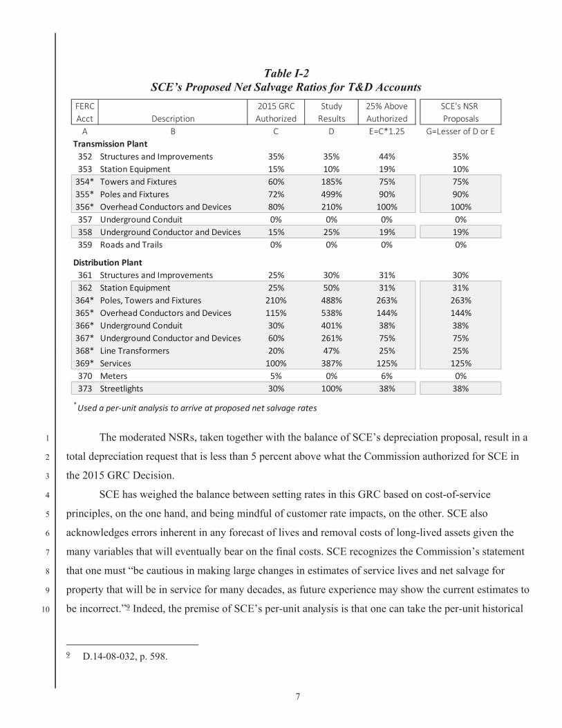
between proposed and authorized NSRs.8 See Table I-2, below, for a summary of SCE’s capping 6

proposal (which was applied only to the accounts with gray highlights given that the study results would 7

have increased the NSRs by more than 25% from authorized rates). 8

7 Id., p. 602. In SCE’s 2015 GRC, the Commission relied on its rationale from the PG&E case, stating that

“[c]onsistent with the logic of gradualism that we applied to PG&E,” it adopted a negative net salvage rate for Account 364 of -210% instead of the -225% that SCE had requested. D.15-11-021, p. 421. Similarly, for Account 369, SCE proposed an increase from -85% to -125%. “Consistent with gradualism,” and for other reasons, the Commission adopted an increase to -100%. Id., p. 425. In SCE’s 2009 GRC, the Commission did not refer to “gradualism” as a doctrine but nonetheless tempered SCE’s otherwise reasonable removal cost estimates “because of economic difficulties facing ratepayers.” D.14-08-032, p. 599 (citing D.09-03-025, pp. 179-180).

8 SCE’s proposal, using the same calculation method as the Commission applied in the 2014 PG&E Decision, is equal to roughly 10% of the difference between currently authorized NSRs T&D accounts and what SCE’s study results would justify.

7

Table I-2 SCE’s Proposed Net Salvage Ratios for T&D Accounts

The moderated NSRs, taken together with the balance of SCE’s depreciation proposal, result in a 1

total depreciation request that is less than 5 percent above what the Commission authorized for SCE in 2

the 2015 GRC Decision. 3

SCE has weighed the balance between setting rates in this GRC based on cost-of-service 4

principles, on the one hand, and being mindful of customer rate impacts, on the other. SCE also 5

acknowledges errors inherent in any forecast of lives and removal costs of long-lived assets given the 6

many variables that will eventually bear on the final costs. SCE recognizes the Commission’s statement 7

that one must “be cautious in making large changes in estimates of service lives and net salvage for 8

property that will be in service for many decades, as future experience may show the current estimates to 9

be incorrect.”9 Indeed, the premise of SCE’s per-unit analysis is that one can take the per-unit historical 10

9 D.14-08-032, p. 598.

FERC 2015 GRC Study 25% Above SCE's NSRAcct Description Authorized Results Authorized ProposalsA B C D E=C*1.25 G=Lesser of D or E

Transmission Plant352 Structures and Improvements 35% 35% 44% 35%353 Station Equipment 15% 10% 19% 10%354* Towers and Fixtures 60% 185% 75% 75%355* Poles and Fixtures 72% 499% 90% 90%356* Overhead Conductors and Devices 80% 210% 100% 100%357 Underground Conduit 0% 0% 0% 0%358 Underground Conductor and Devices 15% 25% 19% 19%359 Roads and Trails 0% 0% 0% 0%

Distribution Plant361 Structures and Improvements 25% 30% 31% 30%362 Station Equipment 25% 50% 31% 31%364* Poles, Towers and Fixtures 210% 488% 263% 263%365* Overhead Conductors and Devices 115% 538% 144% 144%366* Underground Conduit 30% 401% 38% 38%367* Underground Conductor and Devices 60% 261% 75% 75%368* Line Transformers 20% 47% 25% 25%369* Services 100% 387% 125% 125%370 Meters 5% 0% 6% 0%373 Streetlights 30% 100% 38% 38%

*Used a per unit analysis to arrive at proposed net salvage rates

8

cost to remove assets, and apply that per-unit cost to the quantities of assets in the surviving plant 1

balance to obtain a reasonable forecast of the cost to remove the assets given projections about the 2

timing of the assets’ retirements. A key assumption in this analysis is the per-unit cost to retire each 3

asset. While the proposals presented in SCE’s depreciation study substantiate sound estimates of the 4

future costs to retire, SCE does not overlook that future rate cases will provide updates to SCE’s 5

recorded experience that will further refine the expectations of future net salvage. That is, in future rate 6

cases, SCE will have the ability to take its then-surviving plant balances to even better refine its 7

projections about the future in light of then-available conclusions about historical costs-per-unit. By 8

moderating SCE’s depreciation expense, the Commission will make progress towards SCE’s current 9

estimate of forecast net salvage while permitting the Company in future rate cases to rely on additional 10

data to refine its forecasts. 11

D. Summary Tables 12

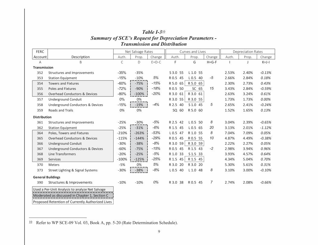
Table I-3, Table I-4, and Table I-5 below summarize the life and net salvage parameters resulting 13

from the analyses described in the chapters below. 14

9

Table I-310 Summary of SCE’s Request for Depreciation Parameters -

Transmission and Distribution

10 Refer to WP SCE-09 Vol. 03, Book A, pp. 5-20 (Rate Determination Schedule).

FERC Net Salvage Rates Curves and Lives Depreciation RatesAccount Description Auth. Prop. Change Auth. Prop. Change Auth. Prop. Change

A B C D E=D C F G H=G F I J K=J ITransmission

352 Structures and Improvements -35% 35% S 3.0 55 L 1.0 55 2.53% 2.40% 0.13%353 Station Equipment -15% 10% 5% R 0.5 45 L 0.5 40 -5 2.66% 2.84% 0.18%354 Towers and Fixtures -60% 75% -15% R 5.0 65 R 5.0 65 2.30% 2.73% 0.43%355 Poles and Fixtures -72% 90% -18% R 0.5 50 SC 65 15 3.43% 2.84% 0.59%356 Overhead Conductors & Devices -80% 100% -20% R 3.0 61 R 3.0 61 2.63% 3.24% 0.61%357 Underground Conduit 0% 0% R 3.0 55 R 3.0 55 1.73% 1.73% 0.00%358 Underground Conductors & Devices -15% 19% -4% R 2.5 40 S 1.0 45 5 2.65% 2.41% 0.24%359 Roads and Trails 0% 0% SQ 60 R 5.0 60 1.52% 1.65% 0.13%

Distribution361 Structures and Improvements 25% 30% -5% R 2.5 42 L 0.5 50 8 3.04% 2.39% 0.65%362 Station Equipment 25% 31% -6% R 1.5 45 L 0.5 65 20 3.13% 2.01% 1.12%364 Poles, Towers and Fixtures 210% 263% -53% L 0.5 47 R 1.0 55 8 7.04% 7.09% 0.05%365 Overhead Conductors & Devices 115% 144% -29% R 0.5 45 R 0.5 55 10 4.87% 4.49% 0.38%366 Underground Conduit 30% 38% -8% R 3.0 59 R 3.0 59 2.22% 2.27% 0.05%367 Underground Conductors & Devices 60% 75% -15% R 0.5 45 R 1.5 43 -2 2.98% 3.94% 0.96%368 Line Transformers 20% 25% -5% R 1.0 33 S 1.5 33 3.93% 4.57% 0.64%369 Services 100% 125% -25% R 1.5 45 R 1.5 45 4.34% 5.04% 0.70%370 Meters 5% 0% 5% R 3.0 20 R 3.0 20 5.30% 5.61% 0.31%373 Street Lighting & Signal Systems 30% 38% -8% L 0.5 40 L 1.0 48 8 3.10% 3.00% 0.10%

General Buildings390 Structures & Improvements 10% 10% 0% R 3.0 38 R 0.5 45 7 2.74% 2.08% 0.66%

Used a Per Unit Analysis to analyze Net Salvage

Moderated as discussed in Chapter 1, Section C

Proposed Retention of Currently Authorized Lives

10

Table I-411 Summary of SCE’s Request for Book Depreciation

Generation Plant

Table I-512 Summary of SCE’s Request for Book Depreciation

General and Intangible Plant

1

11 Id., pp. 5-7. 12 Id., pp. 9-12.

Generation Facility Auth. Prop. Auth. Prop.A B C D E

Nuclear Production Palo Verde 30.5 yrs. 28.0 yrs.Hydro Production 26.0 yrs. 19.9 yrs. $79.3 M $95.3 MOther ProductionPebbly Beach 45 yrs. 25 yrs. $6.6 MMountainview 35 yrs. 35 yrs. $16.3 M $18.5 MPeakers 35 yrs. 35 yrs. $12.1 M $15.1 MSolar Photovoltaic 25 yrs. 20 yrs. $81.9 M $80.9 MFuel Cells 10 yrs. 10 yrs.Energy Storage N/A 10 yrs. N/A

Covered under NDCTP

Life Spans Net Salvage

FERCAccount Description Auth. Prop. Auth. Prop.

A B C D E FGeneral Plant389.2 Easements 60 60 1.67% 1.67%391.1 Office Furniture 20 20 5.00% 5.00%391.2 Personal Computers 5 5 20.00% 20.00%391.3 Mainframe Computers 5 5 20.00% 20.00%391.4 DDSMS Security Monitoring System Various Various 12.90% 9.84%391.5 Office Equipment 5 5 20.00% 20.00%391.6 Duplicating Equipment 5 5 20.00% 20.00%391.7 PC Software 5 5 20.00% 20.00%393 Stores Equipment 20 20 5.00% 5.00%394 Tools &Work Equipment 10 10 10.00% 10.00%395 Laboratory Equipment 15 15 6.67% 6.67%397 Telecommunication Equipment Various Various 9.77% 11.65%398 Misc. Power Plant Equipment 20 20 5.00% 5.00%

Intangible Plant302.020 Hydro Relicensing Various Various 2.52% 2.47%303.640 Radio Frequency 40 40 2.50% 2.50%302.050 Miscellaneous Intangibles 20 20 5.00% 5.00%303.105 Capitalized Software 5 year 5 5 20.00% 20.00%303.707 Capitalized Software 7 year 7 7 14.29% 14.29%303.210 Capitalized Software 10 year 10 10 10.00% 10.00%303.315 Capitalized Software 15 year 15 15 6.67% 6.67%

Lives Depreciation Rates

11

II. 1

COMMISSION DIRECTIVES FROM SCE’S 2015 GRC DECISION 2

In the 2015 GRC Decision, the Commission gave four directives for SCE’s net salvage proposals 3

in this 2018 GRC proceeding. Most of the remainder of this chapter explains SCE’s approach to meeting 4

each of the directives. Section D addresses SCE’s experience with increasingly negative net salvage 5

rates (this testimony refers to “higher” net salvage rates, for simplicity’s sake) and demonstrates how the 6

advancing age of SCE’s infrastructure and the increasing urbanization within its service territory has 7

contributed to more negative NSRs. 8

A. The Four Directives Established in the 2015 GRC Decision 9

Ordering Paragraph 9 of the 2015 GRC Decision required SCE to “provide considerably more 10

detail in support of its net salvage proposals for at least five of the largest accounts, as measured by 11

proposed annual depreciation expense” including at least the following:13 12

The First Directive 13

“A quantitative discussion of historical and anticipated future Cost of Removal (COR) on a 14 per unit basis for the large (greater than 15% as measured by portion of plant balance) asset 15 classes in the account. This discussion should identify and explain the key factors in 16 changing or maintaining the per-unit COR.” 17

The Second Directive 18

“A quantitative discussion of historical and anticipated future retirement mix (i.e., 19 retirements among different asset classes), identifying and explaining the key factors in 20 changing or maintaining this mix.” 21

The Third Directive 22

“A quantitative discussion of the life of assets and original cost of assets being retired, in 23 relation to the COR, on both a historical and anticipated future basis. This discussion should 24 be integrated with and/or cross-reference the proposal for life characteristics.” 25

The Fourth Directive 26

“An account-specific discussion of the process for allocating costs to COR.”14 27

The per-unit analysis required by the Commission involves substantially more work than a “traditional” 28

net salvage analysis that is typically performed by the industry (as described in Standard Practice U-4).15 29

13 D.15-11-021, Ordering Paragraph 9, p. 554. 14 Id., pp. 554-555. 15 For the purpose of this testimony, the term “traditional approach” will be used to describe Standard U-4.

12

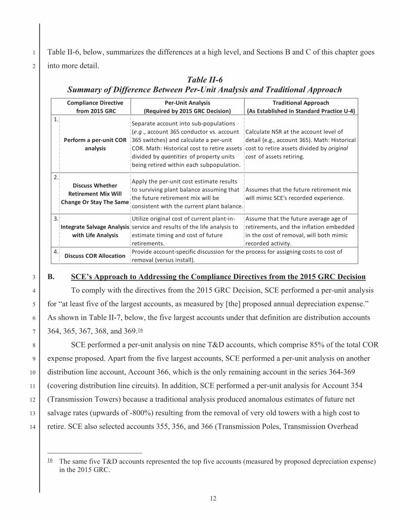
Table II-6, below, summarizes the differences at a high level, and Sections B and C of this chapter goes 1

into more detail. 2

Table II-6 Summary of Difference Between Per-Unit Analysis and Traditional Approach

B. SCE’s Approach to Addressing the Compliance Directives from the 2015 GRC Decision 3

To comply with the directives from the 2015 GRC Decision, SCE performed a per-unit analysis 4

for “at least five of the largest accounts, as measured by [the] proposed annual depreciation expense.” 5

As shown in Table II-7, below, the five largest accounts under that definition are distribution accounts 6

364, 365, 367, 368, and 369.16 7

SCE performed a per-unit analysis on nine T&D accounts, which comprise 85% of the total COR 8

expense proposed. Apart from the five largest accounts, SCE performed a per-unit analysis on another 9

distribution line account, Account 366, which is the only remaining account in the series 364-369 10

(covering distribution line circuits). In addition, SCE performed a per-unit analysis for Account 354 11

(Transmission Towers) because a traditional analysis produced anomalous estimates of future net 12

salvage rates (upwards of -800%) resulting from the removal of very old towers with a high cost to 13

retire. SCE also selected accounts 355, 356, and 366 (Transmission Poles, Transmission Overhead 14

16 The same five T&D accounts represented the top five accounts (measured by proposed depreciation expense)

in the 2015 GRC.

Compliance Directivefrom 2015 GRC

Per Unit Analysis(Required by 2015 GRC Decision)

Traditional Approach(As Established in Standard Practice U 4)

1.

Perform a per unit CORanalysis

Separate account into sub populations(e.g ., account 365 conductor vs. account365 switches) and calculate a per unitCOR. Math: Historical cost to retire assetsdivided by quantities of property unitsbeing retired within each subpopulation.

Calculate NSR at the account level ofdetail (e.g., account 365). Math: Historicalcost to retire assets divided by originalcost of assets retiring.

2.Discuss Whether

Retirement Mix WillChange Or Stay The Same

Apply the per unit cost estimate resultsto surviving plant balance assuming thatthe future retirement mix will beconsistent with the current plant balance.

Assumes that the future retirement mixwill mimic SCE's recorded experience.

3.Integrate Salvage Analysis

with Life Analysis

Utilize original cost of current plant inservice and results of the life analysis toestimate timing and cost of futureretirements.

Assume that the future average age ofretirements, and the inflation embeddedin the cost of removal, will both mimicrecorded activity.

4.Discuss COR Allocation

Provide account specific discussion for the process for assigning costs to cost ofremoval (versus install).

13

Conductor, and Distribution Underground Conduit respectively) given their similarity to corresponding 1

distribution account assets for which SCE conducted a per-unit analysis. 2

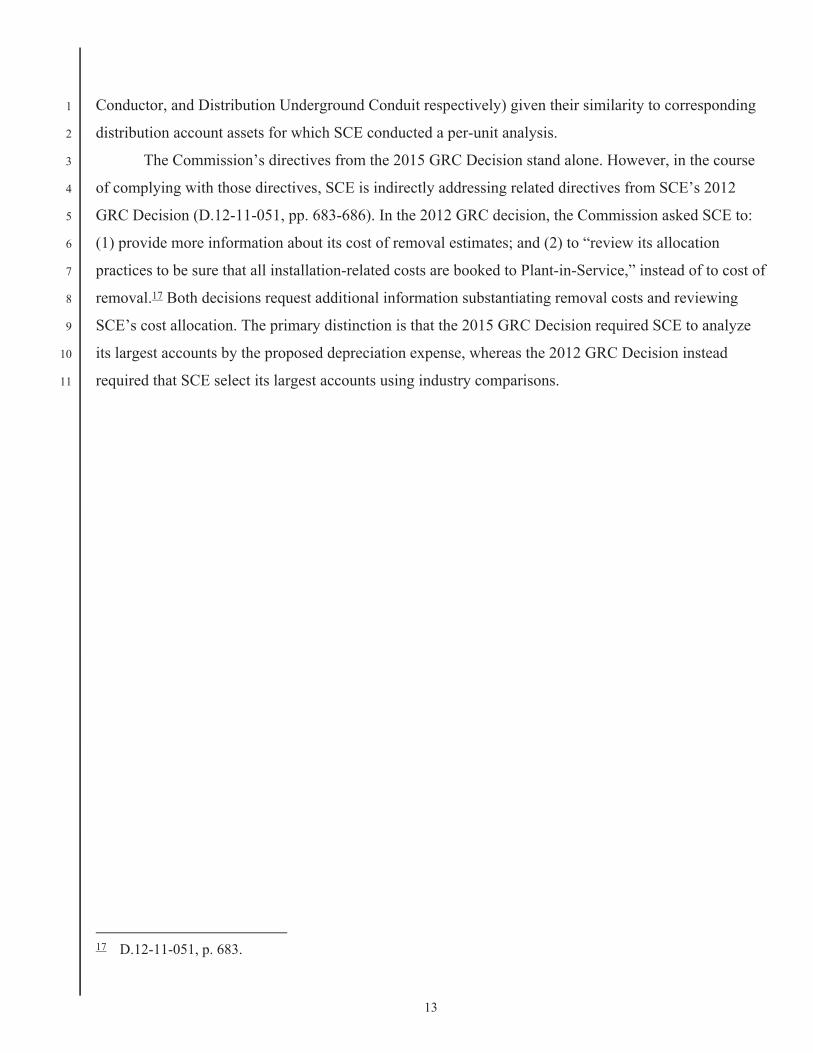
The Commission’s directives from the 2015 GRC Decision stand alone. However, in the course 3

of complying with those directives, SCE is indirectly addressing related directives from SCE’s 2012 4

GRC Decision (D.12-11-051, pp. 683-686). In the 2012 GRC decision, the Commission asked SCE to: 5

(1) provide more information about its cost of removal estimates; and (2) to “review its allocation 6

practices to be sure that all installation-related costs are booked to Plant-in-Service,” instead of to cost of 7

removal.17 Both decisions request additional information substantiating removal costs and reviewing 8

SCE’s cost allocation. The primary distinction is that the 2015 GRC Decision required SCE to analyze 9

its largest accounts by the proposed depreciation expense, whereas the 2012 GRC Decision instead 10

required that SCE select its largest accounts using industry comparisons. 11

17 D.12-11-051, p. 683.

14

Table II-7 T&D Accounts Ranked by Proposed Annual Depreciation Expense

(Based on CPUC-Jurisdictional Depreciation Expense ($M))

1. The First Directive – Per Unit Net Salvage Analysis 1

The per-unit net salvage analysis segments each FERC plant account into large 2

subpopulations (i.e., dollar value of assets representing more than 15% of the total account balance).18 3

To calculate the average per-unit cost to remove, SCE divided the net salvage dollars incurred by the 4

quantity of units retired for each of the identified subpopulations. For example, Account 368—5

18 In the first compliance directive from the 2015 GRC Decision, the Commission referred to “large . . . asset

classes in the account” as measured by 15% or more of the portion of plant balance. D.15-11-021, p. 398. SCE uses the term “subpopulation” to refer to those large asset classes within each FERC account.

FERC ProposedAccount Description Depr. Exp. Rank

Transmission Plant352 Structures and Improvements 5,101 15353 Station Equipment 62,978 6354 Towers and Fixtures 2,603 16355 Poles and Fixtures 19,820 11356 Overhead Conductors & Devices 7,856 13357 Underground Conduit 1,053 17358 Underground Conductors & Devices 6,160 14359 Roads and Trails 114 18

Distribution Plant361 Structures and Improvements 13,783 12362 Station Equipment 45,110 8364 Poles, Towers and Fixtures 174,654 2365 Overhead Conductors & Devices 64,341 5366 Underground Conduit 44,209 9367 Underground Conductors & Devices 218,724 1368 Line Transformers 160,345 3369 Services 65,591 4370 Meters 50,205 7373 Streetlights 26,163 10Total 968,810

Proposals based on results of Per Unit Analysis ($758M or 78% of Total Expense)

15

Distribution Line Transformers—consists of three major subpopulations; overhead (OH) transformers, 1

underground (UG) transformers, and fuseholders. For each subpopulation, SCE divided the net salvage 2

incurred from 2009-201519 by the quantity of units retired, as shown in Figure II-3, below. This per-unit 3

cost to remove each asset formed one part of the basis for forecasting SCE’s expected future net salvage 4

proposals presented in this GRC. 5

a) Traditional Approaches to Analyzing Historical and Future Net Salvage 6

Standard Practice U-4, Determination of Straight-Line Remaining Life 7

Depreciation Accruals (“U-4,” or “Standard Practice U-4”), “sets forth various factors influencing the 8

determination of depreciation accruals and describes methods of calculating these accruals”20 with the 9

purpose of assisting “the Commission staff in determining proper depreciation expenses.”21 Although 10

over 50 years old, Standard Practice U-4 represents conventional utility depreciation practices. The 11

depreciation rates proposed in this study are consistent with the standard practices described in U-4. In 12

addition, SCE conducted a more rigorous per-unit analysis for nine T&D accounts in response to the 13

Commission’s directives from the 2015 GRC. 14

To meet requirements set forth in U-4, SCE uses different approaches to estimate 15

NSRs based on the plant’s retirement characteristics and recorded experience. Broadly speaking, SCE’s 16

net salvage study analyzes mass property differently than life-span property and other non-mass plant 17

accounts. Mass property accounts (e.g., transmission and distribution plant accounts) are those that have 18

a significant number of property units which are generally retired separately. Life-span property refers to 19

accounts which are comprised of a few major units which individually are expected to retire at a single 20

point in time (e.g., generating plants). 21

Mass property plant accounts, such as T&D, can contain a significant number of 22

components and generally experience large numbers of retirement transactions under a diverse number 23

of retirement circumstances. The large number of retirement units and retirement occurrences for mass 24

property generally necessitate an analysis of aggregate historical NSRs and per-unit costs. To 25

accomplish this, Standard Practice U-4 describes how to estimate future net salvage rates using the 26

19 This period contains detailed net salvage data by CPR, available in PowerPlan, SCE’s capital system of

record. Net salvage data prior to this period is maintained at the FERC prime account level only. 20 Standard Practice U-4 is available at

http://docs.cpuc.ca.gov/PublishedDocs/Published/G000/M042/K177/42177433.PDF and includes methods to analyze net salvage.

21 Id., p. 6.

16

experienced ratios of net salvage, gross salvage, and removal cost (in today’s dollars) as a percent of the 1

original installed costs (in older dollars) of retirements. The average net salvage rate by FERC account is 2

then applied to the total plant balance to determine the estimated future net salvage amount, barring any 3

adjustments. Understanding the inputs involved in the calculation and the calculation itself is important 4

to interpreting the resulting NSRs. The calculations are as follows: 5

Figure II-2 Computing NSRs Under the Traditional Approach

b) Comparing the Differences Between Calculating Net Salvage Ratios Using a 6

Traditional Analysis Versus Per-Unit Analysis 7

The first and most important way that a per-unit analysis differs from the 8

traditional analysis is that the NSRs are computed using the original cost of the surviving plant balance 9

(i.e., the current plant balance), as opposed to a traditional analysis’ use of the original cost of the plant 10

that has already retired. That is, a traditional net salvage analysis examines the historical NSRs as the 11

principal factor used to estimate future NSRs. By contrast, the per-unit analysis takes historical per unit 12

costs and applies them to surviving plant quantities to project future removal costs given projections 13

(from the life analysis) of when assets are expected to retire. The traditional approach implicitly assumes 14

that factors such as the age of retirements, changes in SCE’s operating environment, levels of inflation 15

and other factors will, in the future, be the same as they were in the past. By contrast, a per-unit analysis 16

develops forward-looking estimates of net salvage by relying on recorded costs, surviving plant 17

balances, and assumptions about the timing of future retirements. 18

An illustration of SCE’s approach to the per-unit analysis computation is 19

instructive, especially compared to the calculation in Figure II-2, above. First, the net salvage cost per-20

unit is calculated by summing seven years’ worth of recorded history—in both dollars used to remove 21

assets, and quantities of assets removed—to arrive at a per-unit net salvage value by sub-population: 22

Net Salvage % = Gross Salvage % Removal Cost %

Net Salvage ($) Gross Salvage ($) Removal Cost ($)Retirements ($) Retirements ($) Retirements ($)

=

17

Figure II-3 Calculation of Per-Unit Net Salvage Costs

(Recorded 2009-2015 values for Account 368 – Line Transformers)

Next, the per-unit cost derived above is applied to a forecast using anticipated 1

rates of inflation, as opposed to inflation experienced in the past. A simplified (no-inflation) calculation 2

of future net salvage is shown in Figure II-4, as it shows the per-unit net salvage from Figure II-3 3

multiplied by the year-end 2015 surviving quantities (the study date). The resulting value is equivalent 4

to an estimate of the cost to remove all of the assets in Account 368 as of the study date. 5

Figure II-4 22 Calculation of Future Net Salvage Using a Per-Unit Methodology

(for Account 368 – Line Transformers; excluding future inflation)

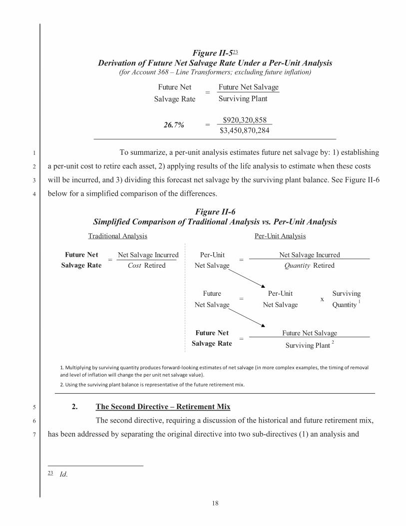
This forecast of future net salvage can be divided by the costs of assets currently 6

serving customers (the denominator, or surviving plant balance) to arrive at an estimated future NSR. 7

This no-inflation estimate of the future NSR is shown in Figure II-5 below. 8

22 Refer to WP SCE-09 Vol. 03, Book A, pp. 21-24 (Per-Unit Calculations).

Per-UnitNet Salvage

Overhead UndergroundTransformer Transformer Fuseholder Others

Per-Unit $79,500,742 $78,642,058 $44,409,667 $19,071,340Net Salvage 141,838 53,904 275,472 19,862

= $560.50 $1,458.93 $161.21 $960.19

=

=Net Salvage ($)Quantity Retired

Overhead UndergroundTransformer Transformer Fuseholder Others

$560.50 $1,458.93 $161.21 $960.19x x x x

456,611 259,299 1,400,640 62,788

$920,320,858 = $255,932,428 $378,298,499 $225,801,375 $60,288,556

+

Future Net Salvage =

Per-Unit NSx

Per-Unit Surviving Quantity

Future Net Salvage = + +

18

Figure II-523 Derivation of Future Net Salvage Rate Under a Per-Unit Analysis

(for Account 368 – Line Transformers; excluding future inflation)

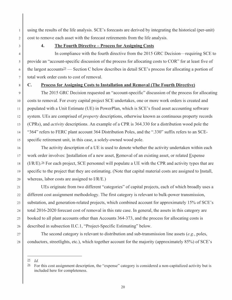
To summarize, a per-unit analysis estimates future net salvage by: 1) establishing 1

a per-unit cost to retire each asset, 2) applying results of the life analysis to estimate when these costs 2

will be incurred, and 3) dividing this forecast net salvage by the surviving plant balance. See Figure II-6 3

below for a simplified comparison of the differences. 4

Figure II-6 Simplified Comparison of Traditional Analysis vs. Per-Unit Analysis

2. The Second Directive – Retirement Mix 5

The second directive, requiring a discussion of the historical and future retirement mix, 6

has been addressed by separating the original directive into two sub-directives (1) an analysis and 7

23 Id.

Future Net Future Net SalvageSalvage Rate

$920,320,858$3,450,870,284

=Surviving Plant

26.7% =

Future Net Net Salvage Incurred Per-UnitSalvage Rate Cost Retired Net Salvage

Future Per-Unit SurvivingNet Salvage Net Salvage Quantity 1

Future NetSalvage Rate

Traditional Analysis

= =

Per-Unit Analysis

Quantity RetiredNet Salvage Incurred

1. Multiplying by surviving quantity produces forward looking estimates of net salvage (in more complex examples, the timing of removaland level of inflation will change the per unit net salvage value).

2. Using the surviving plant balance is representative of the future retirement mix.

Surviving Plant 2

= x

=Future Net Salvage

19

discussion of the historical retirements, and (2) a discussion of the expected future retirement mix. The 1

per-unit analysis described above complies with the first sub-directive because it requires review of the 2

historical mix of retirements to determine an average per-unit cost to retire. To address the second sub-3

directive, SCE assumes that the future retirement mix will be consistent with the asset mix in the 4

surviving plant balance as of year-end 2015. (In future rate cases, when the retirement mix changes, the 5

forecast NSR will change accordingly.) 6

Analyzing the account by subpopulation achieves a more detailed “weighting” than 7

looking at the account-based retirement mix in the aggregate. That is, the traditional approach focuses 8

solely on the backward-looking ratios, which are used to estimate future net salvage. The blunt 9

assumption underlying this approach is that the mixture of asset retirements in the past is representative 10

of what one could expect in the future without regard to the composition of the then-current plant 11

balance. Under the per-unit approach, by contrast, one focus is on the surviving plant balance, which 12

offers a “snapshot” in real time that forms the basis for estimating the future mix of retirements. In 13

determining its proposed depreciation expense, SCE did not identify or rely on factors that would cause 14

it to modify the future retirement mix relative to the mix that currently exists in its plant accounts. 15

Should factors in the future modify the retirement mix, the surviving plant balances examined at the 16

relevant time will integrate and reflect those changes. 17

3. The Third Directive – The Age of Retirements and Integration of Salvage and Life 18

Analyses 19

The third directive requires SCE to provide a quantitative discussion of the life of assets 20

and original cost of assets being retired in relation to the cost of removal. This directive has been 21

addressed by separating the original directive into two sub-directives requiring (1) a discussion of the 22

age of retirements experienced and (2) a forecast of the future age of retirements given the results of the 23

life analysis. The Commission intended this directive to “integrate” the life analysis with the COR 24

analysis: “This [COR] discussion should be integrated with and/or cross-reference the proposal for life 25

characteristics.”24 The only way to properly integrate both prongs of the analysis is to factor in the 26

impact of the passage of time, or inflation, on the per-unit costs. To address this directive, SCE has 27

provided the average age and original cost of assets retired, together with a forecast of future retirements 28

24 D.15-11-021, p. 398 (see also Ordering Paragraph 9.i., pp. 554-555).

20

using the results of the life analysis. SCE’s forecasts are derived by integrating the historical (per-unit) 1

cost to remove each asset with the forecast retirements from the life analysis. 2

4. The Fourth Directive – Process for Assigning Costs 3

In compliance with the fourth directive from the 2015 GRC Decision—requiring SCE to 4

provide an “account-specific discussion of the process for allocating costs to COR” for at least five of 5

the largest accounts25 — Section C below describes in detail SCE’s process for allocating a portion of 6

total work order costs to cost of removal. 7

C. Process for Assigning Costs to Installation and Removal (The Fourth Directive) 8

The 2015 GRC Decision requested an “account-specific” discussion of the process for allocating 9

costs to removal. For every capital project SCE undertakes, one or more work orders is created and 10

populated with a Unit Estimate (UE) in PowerPlan, which is SCE’s fixed asset accounting software 11

system. UEs are comprised of property descriptions, otherwise known as continuous property records 12

(CPRs), and activity descriptions. An example of a CPR is 364.330 for a distribution wood pole the 13

“364” refers to FERC plant account 364 Distribution Poles, and the “.330” suffix refers to an SCE-14

specific retirement unit, in this case, a solely-owned wood pole. 15

The activity description of a UE is used to denote whether the activity undertaken within each 16

work order involves: Installation of a new asset, Removal of an existing asset, or related Expense 17

(I/R/E).26 For each project, SCE personnel will populate a UE with the CPR and activity types that are 18

specific to the project that they are estimating. (Note that capital material costs are assigned to Install, 19

whereas, labor costs are assigned to I/R/E.) 20

UEs originate from two different “categories” of capital projects, each of which broadly uses a 21

different cost assignment methodology. The first category is relevant to bulk-power transmission, 22

substation, and generation-related projects, which combined account for approximately 15% of SCE’s 23

total 2016-2020 forecast cost of removal in this rate case. In general, the assets in this category are 24

booked to all plant accounts other than Accounts 364-373, and the process for allocating costs is 25

described in subsection II.C.1, “Project-Specific Estimating” below. 26

The second category is relevant to distribution and sub-transmission line assets (e.g., poles, 27

conductors, streetlights, etc.), which together account for the majority (approximately 85%) of SCE’s 28

25 Id. 26 For this cost assignment description, the “expense” category is considered a non-capitalized activity but is

included here for completeness.

21

total 2016-2020 forecast COR in this rate case. At a high level, the assets in this second category 1

(sometimes referred to as “mass plant” assets) are booked to Accounts 364 to 373, and the process for 2

assigning costs is described in subsection II.C.2., “Design Manager (DM) Estimating” below. 3

1. Project-Specific Estimating (Bulk-Power Transmission, Substation, and 4

Generation/Other) 5

For project-specific estimating, SCE personnel create a detailed cost estimate for each of 6

the activities required at the outset of each job. The cost estimate reflects the total estimated costs of 7

installation separate from the total estimated costs of removal. 8

a) Bulk Power Transmission and Substation (Accounts 350-359 and 362) 9

For bulk power transmission and substation estimates,27 engineers and technical 10

experts use the Scope and Cost Management Tool (SCMT) to document, track, and communicate the 11

scope for each project. Cost estimators then complete the costs for each project identifying and 12

separating the installation, removal and expense activities. They assign CPR accounts that serve as the 13

basis for creating the UEs that will ultimately be uploaded into the PowerPlan system. 14

For example, a capital project to replace a bulk power (e.g., 500/220 kV) 15

transformer begins when the estimator develops a specific cost estimate by itemizing the scope of major 16

activities (e.g., removing the old transformer, trench cover, power/control cable, conduits, etc. and then 17

installing the new equipment).28 The installation and removal activities are separately identified by hours 18

required to install and/or remove the particular assets. In other words, there is a specific estimate of the 19

labor, equipment, and associated overheads required to remove assets, and it is not a template-based 20

“allocation” of total hours required for the job. The work is also broken out by the specific classification 21

of employee who will be performing the task and also whether or not SCE crews or contract crews will 22

be performing the work. The details of this estimate are compiled and used to create the UE in 23

PowerPlan that will assign the ultimate costs recorded as “installation” costs versus “removal” costs. 24

b) Generation and Other (Accounts 301-348, and 390-398) 29 25

Generation, Information Technology, and Operational Services also use project-26

specific estimating. That is, a detailed scope of work is set by engineers and other technical experts. The 27

27 Examples of accounts with related assets are Accounts 350 to 359 and 362. 28 Refer to WP SCE-09 Vol. 03, Book A, pp. 25-41 (Project-Specific Estimating) for an example of a project-

specific estimate. 29 Examples of some of these accounts are: Accounts 301 to 348 and 390 to 398.

22

scope of work is separated into installation and removal activities and becomes the foundation for 1

building the UEs that are put in the PowerPlan System. 2

2. Design Manager (DM) Estimating (Distribution/Sub-Transmission Assets) 3

For the large majority of capital assets, such as distribution and some sub-transmission 4

line assets (e.g., poles, conductors, streetlights, etc.), it is impractical for SCE to use project-specific 5

estimating every time a new capital project is undertaken. That is because in any given year, SCE will 6

install and replace thousands of these units of property. For example, in 2015 alone, SCE replaced over 7

40,000 wood poles, 25,000 transformers, and 3,000 miles of conductor.30 8

To manage the high volume of work, SCE uses a template-based estimating approach to 9

assign a capital project’s total costs to Installation, Removal, and Related Expense (I/R/E). Since 2010, 10

SCE’s planners have been using Design Manager to estimate labor hours, schedule work, and price 11

distribution and sub-transmission projects. The DM estimating approach is commonly used for 12

emergency work, planned/routine work, and customer-driven projects including relocations, 13

overhead/underground conversions, new service connections and meter installations. A subset of data 14

from DM is sent to PowerPlan, and that is where SCE’s allocation methodology is applied for fixed 15

asset accounting purposes, as explained in more detail below. 16

a) Building a Project Estimate in DM Using Compatible Units (CUs) 17

A planner tasked with initiating a project (e.g., a pole replacement) will open a 18

work order and, based on the project scope (including site visits, where applicable), begin identifying 19

Compatible Units (CUs) required to complete the job. CUs are building blocks of material and labor 20

used to develop the distribution design and work order cost estimates. They eliminate the need for 21

planners to manually identify and select every material component for frequently installed equipment 22

and structures on SCE’s electrical system. CUs identify the quantity and type of property needed for a 23

project (e.g., wood poles, transformers, conductors, etc.) and associated estimates of labor hours and 24

costs. DM contains legend codes to indicate the type of activity to be performed for each asset (i.e., 25

installation vs. removal). DM incorporates the use of over 4,500 distribution CUs, to help planners build 26

cost estimates and schedule work depending on the requirements of the job. 27

30 Refer to WP SCE-09 Vol. 03, Book D, pp. 2-40 (Per-Unit Net Salvage Analysis). Estimates are taken from

per-unit analysis quantity.

23

b) Cost Allocation in PowerPlan 1

For purposes of fixed asset accounting, the CUs and legend codes from DM work 2

orders are migrated to PowerPlan. CUs are paired with—and converted to—one of over 100 CPR 3

accounts.31 At this point, the CPR account consists only of quantities and types of property to be 4

installed and, if applicable, quantities and types of property to be removed. The estimated costs and 5

labor hours from DM are not carried over to PowerPlan. For fixed asset accounting purposes, SCE uses 6

a “Standard Rates Table”32 to allocate installation and removal costs relative to total project costs of 7

individual work orders. The Standard Rates Table is also used to allocate costs among the appropriate 8

FERC accounts. 9

Each CU relates to a specific, individual piece of property. For example, different 10

CUs are used to reflect the various height, class, material, and treatment status33 of poles. Likewise, 11

different CUs are used to reflect the various size, voltage and even manufacturer of transformers. The 12

number of CUs that planners use to build a UE is many times greater than the number of CPRs to which 13

the CUs are paired in PowerPlan. The Standard Rates Table allocation is therefore performed at an 14

aggregated level that accounts for the various types of property the CPRs encompass. The table has been 15

in continuous use since approximately the 1970s and it sets forth allocation factors that have been 16

studied but that have not been materially modified over the years. However, in Chapter II.C.2.c., SCE 17

describes three studies validating that the Standard Rates Table’s general allocations continue to be 18

reasonable, if not more conservative in assigning costs to removal versus installation. 19

An example of how the Standard Rates Table works in PowerPlan is illustrated in 20

the three tables below, Table II-8, Table II-9, and Table II-10. Assume that a project to replace a wood 21

pole also requires replacing an attached streetlight fixture. The table below lists the CPRs and the 22

associated allocation factors by activity:34 23

31 A CPR account is defined as the combination of a FERC plant account and a retirement unit subaccount. 32 In prior rate cases, this “Standard Rates Table” has sometimes been referred to as “Table 34.” 33 Treatment processes vary and are used to minimize pole decay (e.g., through-boring, treatments, etc.). 34 Note that the numbers are neither dollars nor hours; they are allocation factors from the Standard Rates Table.

Refer to WP SCE-09 Vol. 03, Book A, pp. 47-51 (Standard Rates Table).

24

Table II-8 Standard Rates Table Values

The Standard Rates Table values are not important as absolute values; they are 1

only meaningful in relation to each other. In the example above, the value assigned to removing the pole 2

(600) is—appropriately—much larger than the value assigned to removing the fixture (74). 3

Table II-9 below converts the values in the rows and columns above to 4

percentages of the total. Comparing the values across columns shows the allocation between install and 5

removal. Comparing the values between rows shows the allocation between CPR accounts. 6

Table II-9 Percent of Sum of Standard Rates

For fixed asset accounting purposes, the percentages from the table above are 7

applied to the allocable dollars35 in the project’s work order, as shown in Table II-10 below. 8

35 Material costs are generally allocated to installation, not removal.

CPRAccount Description364.330 Distribution Wood Pole 1,286 600 1,886

+ +373.390 Streetlight fixture 105 74 179

= =Total 1,391 674 2,065=

+

+

+

Install RemovalStandard Rates Table Values

Total=

=

CPRAccount Description364.330 Distribution Wood Pole 62% 29% 91% Allocation

+ + between CPR373.390 Streetlight fixture 5% 4% 9% Accounts

= =Total 67% 33% 100%

Allocation between Install and Removalfor replacement project

Percent of Sum of Standard Rates ValuesInstall Removal Total

+ =

+ =

+ =

25

Table II-10 Application of Standard Rates to $1,000 of Labor

As illustrated in Table II-8, Table II-9, and Table II-10 above, while the Standard 1

Rates Table uses a template approach to setting allocation factors, the resulting cost assignment for each 2

project is “customized” in several ways. First, by virtue of the planner’s initial designation of CU legend 3

codes, the activity for each CPR is appropriately designated as “installation” versus “removal,” and these 4

splits are specific to each project depending on the properties and quantities that are installed or 5

removed. Second, the quantities of property estimated by planners are drawn into PowerPlan and trued 6

up by the end of every project to reflect what was actually removed and installed. Third, and most 7

importantly, as units of property and quantities change with each work order, the matrix of cost 8

assignment becomes more complex and reflective of the work performed in that project. For example, if 9

another CPR account were added to the illustration above, the resulting allocations would be modified to 10

reflect the weight of each CPR account relative to the total. 11

3. Substantiating SCE’s Standard Rates Table Allocation Factors 12

SCE has conducted three studies substantiating the results of the Standard Rates Table’s 13

installation and removal allocation factors—in 2004, 2006, and 2016. The results of these three studies 14

are summarized in Table II-11, which shows the CORs as a percentage of total costs under the Standard 15

Rates Table compared to the COR percentages from the 2004, 2006 and 2016 Studies. The table 16

demonstrates that SCE’s allocation practice continues to be reasonable and appropriate. In fact, the 17

Standard Rates Table COR allocations (on which the proposals for depreciation expense are based) are 18

the most conservative with respect to removal costs given that the study results indicate that more 19

dollars could be assigned to removal using cost assignment data from field experts. 20

CPRAccount Description364.330 Distribution Wood Pole $623 $290 $913

+ +373.390 Streetlight fixture $51 $36 $87

= =Total $674 $326 $1,000

TotalRemovalInstall+ =

+ =

+ =

Application of Standard Rates to $1,000 of Labor

26

Table II-1136 Comparison of Cost Assignment Ratios Across Three Studies Relative to the Standard

Rates Table (Stated as Percentage of Total Cost)

a) 2004 Study 37 1

In the 2004 Study, performed for the 2006 GRC, SCE assembled field operations 2

experts who compiled and analyzed work requirements for replacement projects of various assets under 3

many different scenarios. The 2004 Study approached replacement costs from the perspective of SCE 4

operations and maintenance personnel who had an average of 21 years of experience working with T&D 5

assets. These subject matter experts, who had experience performing and supervising work activities, 6

reviewed and assessed the time and work requirements for each of several scenarios including total time 7

spent on the project, equipment requirements, and crew size requirements. The work activities were 8

evaluated and separated into installation and removal activities. The experts compared the results from 9

the study to the existing allocations in the Standard Rates Table and determined that no update to the 10

Standard Rates Table was required because the estimated costs of removal were not overstated using the 11

existing process. 12

36 The nine accounts listed on this table are the same ones for which SCE performed a per-unit analysis. Refer to

WP SCE-09 Vol. 03, Book A, pp. 42-46 (Summary of Study Results). 37 Refer to WP SCE-09 Vol. 03, Book A, pp. 52-172 (2004 Study Results).

FERC Standard 2004 2006 2016Account Description Rates Table Study Study StudyTransmission Plant

354 Towers and Fixtures355 Poles and Fixtures 27.2% 30.2% 31.4% Not Studied356 Overhead Conductors & Devices 42.1% 56.1% 56.7% Not Studied

Distribution Plant364 Poles, Towers and Fixtures 36.6% 43.0% 39.4% 46.1%365 Overhead Conductors & Devices 34.7% 38.6% 37.1% 35.6%366 Underground Conduit 20.0% 42.3% 41.9% 41.7%367 Underground Conductors & Devices 34.7% 32.1% 33.7% 35.7%368 Line Transformers 27.3% 47.4% 48.8% 41.6%369 Services 35.5% 44.2% 44.5% 33.8%

Weighted Average* 33.0% 38.8% 38.3% 37.5%

*Weighted by 2009-2015 Recorded Net Salvage

Not Applicable - Non-Mass Plant

27

In preparing this testimony, SCE revisited the rebuttal testimony of its outside 1

depreciation expert from the 2015 GRC. Appendix A of the witness’s rebuttal testimony was a copy of 2

the 2004 study, and, in response to a question about the “historical documentation describing . . . the 3

development of allocation factors used by SCE,” the witness referred to the 2004 study in Appendix A 4

(among other things) as evidence that “SCE used a very robust and detailed process to develop its 5

allocation factors.”38 As a point of clarification, the allocation factors to which the witness referred in his 6

testimony are not the Standard Rates Table allocations that formed the basis of SCE’s depreciation 7

request in the 2015 GRC and this 2018 GRC.39 Rather, the witness testified to the allocation process and 8

results from the 2004 Study together with his own observations and discussions with field personnel 9

about cost assignment. Any lack of clarity in distinguishing between the Standard Rates Table 10

allocations and the 2004 Study’s allocations is not material as demonstrated in Table II-11, above. In 11

fact, the results of the 2004 Study would have assigned a larger percentage of costs to removal than does 12

the Standard Rates Table (by approximately 5%), as shown in that table. 13

b) 2006 Study 40 14

In 2006, SCE updated the 2004 Study in preparation for the 2009 GRC. Using a 15

similar approach to the one utilized for the 2004 Study, SCE assembled a team of field operations 16

experts to gather consensus estimates for labor hours for the job configuration scenarios used in the 2004 17

Study. The panel of study participants included overhead and underground experts from metropolitan 18

and rural areas of SCE’s service territory and others who reviewed job conditions, crew sizes, and labor 19

hour estimates. In addition, as an enhancement to the 2004 Study, the field experts weighted the 20

installation and removal activities by the likelihood of the scenarios’ occurrence in the field. The results 21

from the analysis were compared to the Standard Rates Table allocations, and the experts determined 22

that if they were to update the Standard Rates Table allocations to incorporate the results of the 2006 23

Study, the cost of removal allocations would increase by over 5%. For this reason, and because SCE 24

planned to implement new work planning and accounting software in 2010, SCE elected to continue 25

using the Standard Rates Table. 26

38 2015 GRC, SCE-26, Volume 3, p. 13. Later in the same volume, SCE’s witness testified that the study in

Appendix A shows that “the allocation factor will change based on more complex installations.” Id., p. 115 (emphasis in original). This was a reference to the study results, not to the way in which the Standard Rates Table allocations are applied today.

39 The Standard Rates Table was used to assign costs for several GRCs even prior to 2015. 40 Refer to WP SCE-09 Vol. 03, Book A, pp. 173-188 (2006 Study Results).

28

c) 2016 Study 1

(1) Background of Development of Compatible Units (CUs). 2

Before explaining the results of the 2016 Study, it is important to 3

understand the development beginning in 2009 of the CUs that T&D employees use to plan, estimate, 4

schedule and bill work. As explained in section II.C.2, above, DM incorporates the use of over 4,500 5

distribution CUs to assist planners with building cost estimates and scheduling work depending on the 6

specific requirements of the job. When CUs are migrated to PowerPlan, they are mapped to CPRs and, 7

for fixed asset accounting purposes only, the Standard Rates Table is used to allocate costs between 8

removal and installation. The labor hours embedded in the CUs in DM are not used in the cost allocation 9

process, but are important to facilitating the planning, scheduling, execution and closure of work orders 10

for the T&D Operating Unit. 11

(2) 2009-2010 Labor Study 12

In 2009-2010, SCE undertook a year-long process to review and update 13

the precursors to CUs, called “assembly kits,” in preparation for integration into DM and SAP. This 14

effort to examine CU hours was internally referred to as the “Labor Study,” and it leveraged the results 15

of the 2004 and 2006 Studies described above. The participants in the Labor Study—including 16

construction managers and supervisors, foremen, trouble men, and standards and engineering teams 17

from across SCE’s service territory41 — examined over 4,500 CUs of distribution assets and modified 18

1,800 of them.42 The purpose was not to modify CUs for depreciation plant accounting purposes; rather, 19

the intent of the study was to refine the “building blocks” of SCE’s thousands of work orders (CUs) to 20

improve planning, crew scheduling, estimating and pricing jobs and work order closure processes. 21

For three to four months of eight-hour days, the teams went line-by-line 22

through SCE’s old Material Management System (the old mainframe system in which the assembly kits 23

resided) to remove obsolete items.43 The initial part of the Labor Study was devoted to just clearing 24

SCE’s planning system of obsolete assembly kits. In the latter phase, the teams updated the labor hours 25

41 Specifically, the experts came from the Metro West, Metro East, North Cost, Desert and Orange areas of

SCE’s service territory. 42 Separately, approximately 3,900 CUs for substation and sub-transmission assets were reviewed and migrated

into SAP. 43 For example, if the Material Management System referred to a transformer with certain voltage requirements

that were no longer applicable, that assembly kit was removed.

29

of the most commonly used CUs—transformers, switches and poles. The goal was to approximate labor 1

hours as precisely as possible in order to improve crew scheduling times and cost estimates.44 The team 2

based labor hour estimates on the expert judgment and analysis of T&D employees, taking into 3

consideration factors such as crew size, whether the work is performed energized, and whether the crews 4

would have vehicle access. The work also involved examining individual CUs to assign updated 5

removal and installation hours. The end result of the panel of experts’ process was to review—and, if 6

necessary, revise—the installation and removal hours (the removal hours assigned in the old assembly 7

kits had been set at roughly half of installation hours). The updated labor values were developed using 8

an average of the best, typical and worst case scenario specific to the installation and removal of a CU. 9

By 2010, the update process for the CUs had been completed, but SCE 10

uses an ongoing governance structure to further update CUs on an ad hoc basis when required. There are 11

three full-time employees whose job is focused on maintaining and updating CUs so that 12

proposed/required changes flow through a standard process. The CU team receives an average of 22 13

requests each year to create new CUs (from planning, engineering, apparatus and meter services). The 14

team also receives approximately 60 requests each year to review the accuracy of specific CUs 15

(requesting review of hours or material components). Of the approximately one thousand field requests 16

that have come through to examine CUs since 2010, less than a handful of requests actually resulted in 17

changes to the installation/removal hours. This is due both to the comprehensiveness of the 2009-2010 18

Labor Study and the reality that work processes/practices do not change so significantly over time as to 19

impact cost of removal ratios. 20

When planners use CUs to design and estimate particular jobs, they may—21

based on their own experience or through discussions with field personnel—supplement the labor 22

estimates with additional Install, Removal or Expense labor hours on a work order-by-work-order basis. 23

Any changes made to the project based on job complexity, additional crew tailboards, additional traffic 24

control requirements, travel time, etc. are used for that specific work order only, and do not result in 25

updating the master CU in the CU library. Updates to the CUs in the CU library occur occasionally. For 26

example, in August 2012, a manager within the Street and Outdoor Lighting Organization requested that 27

the CU team review the installation hours for street light photocells given his assessment that the 0.5 28

44 Work under Rules 2, 15, 16 and 20 benefit from accurate cost estimates built into CUs because those

estimates form the basis for how customers are billed.

30

man hours for installation of this CU appeared high. The CU team pulled together a team of subject 1

matter experts to assess and recommend a revision to the hours and determined that it should be reduced 2

to 0.1 hours. Upon approval, the update was made in DM. 3

(3) 2016 Comparison of Standard Rates Table and CUs 4

In 2016, SCE undertook a study comparing the Standard Rates Table 5

allocations with what the allocations would be if SCE’s fixed asset accounting process mapped the CU 6

process described above. The scope of the study included a review of over 70,000 individually planned 7

distribution orders developed in Design Manager in 2015, which collectively amounted to $1.7 billion, 8

or approximately 84% of that year’s capital expenditures. The review included comparing the 9

installation and removal cost allocation from DM against the Standard Rates Table allocation for all 10

70,000 orders. The results indicate that the planners’ CU-based approach, which is more detailed than 11

the higher-level aggregation of the CPR-based allocations in the Standard Rates Table, results in cost 12

assignments substantially similar to the Standard Rates Table (validated by the 2004 and 2006 Study 13

results based on the panels of T&D experts).45 14

D. SCE’s Experience with Increasingly Negative Net Salvage Rates 15

NSRs are typically negative because gross salvage is largely negligible compared to the cost of 16

removal. The main reason for more negative NSRs can be attributed to the results of this mathematical 17

formula: (1) costs to retire assets (numerator) in today’s dollars divided by (2) the age and original cost 18

of assets retired (denominator). Since 2002, SCE’s 5-year rolling average NSR has more than tripled for 19

distribution infrastructure, from -66% to -283% as shown in Figure II-7 below. 20

45 Refer to WP SCE-09 Vol. 03, Book A, pp. 189-197 (2016 Study Results).

31

Figure II-7 Realized Net Salvage Ratios

Distribution Plant 2002-2015

For the last twenty years, SCE has experienced increasingly negative net salvage ratios for reasons 1

explained in the next sections. 2

1. The Average Age of Retirements is Increasing 3

a) Age and Inflation Impacts on Recorded Net Salvage Ratios 4

An important consideration for the net salvage ratio calculation is that the 5

numerator (net salvage cost) and the denominator (original cost) are stated in dollars spent at different 6

points in time. The original cost retired in the denominator are measured in dollars from the time the 7

plant was first placed in service (i.e., older dollars) and the net salvage amounts in the numerator are 8

measured when the plant is retired from service (i.e., using more recent dollars). For example, a 9

distribution pole placed into service in 1970 and retired in 2015 will have an original cost stated in 1970 10

dollars, but the removal costs will be incurred using 2015 dollars. Consequently, the temporal distance 11

between installation and removal can have a significant effect on net salvage ratios primarily due to the 12

effects of inflation. The effects of inflation are most apparent in the removal cost ratio, as the cost to 13

retire (i.e., labor) is what is subject to the forces of inflation.46 14

46 Refer to WP SCE-09 Vol. 03, Book A, pp. 198-201 (Experienced Net Salvage Rates) - Depreciation Systems,

Frank K. Wolf and W. Chester Fitch, Iowa State University Press, pp. 53-55.

66.5%

238.3%

300.0%

250.0%

200.0%

150.0%

100.0%

50.0%

0.0%2002 2003 2004 2005 2006 2007 2008 2009 2010 2011 2012 2013 2014 2015

NetSalvageRatio

Year

Growth in Net Salvage Ratios 10.31%

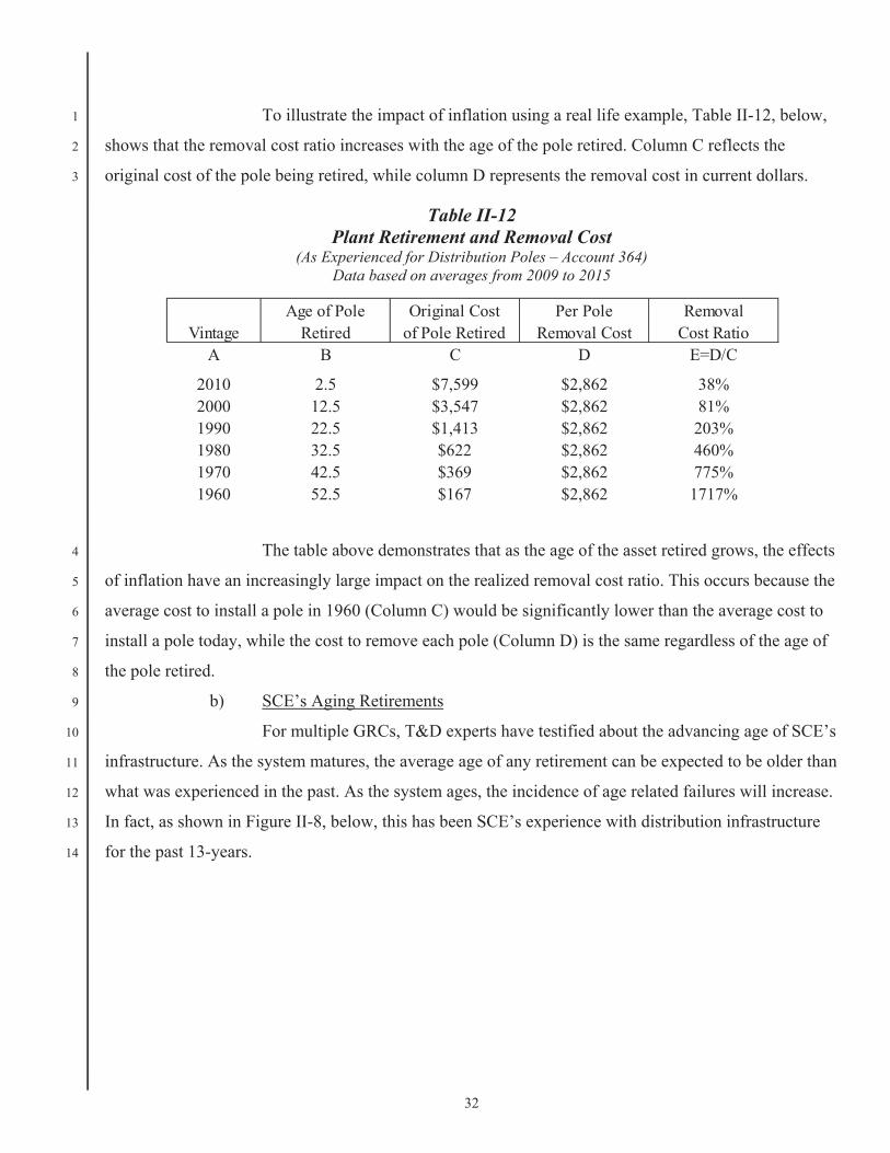
32

To illustrate the impact of inflation using a real life example, Table II-12, below, 1

shows that the removal cost ratio increases with the age of the pole retired. Column C reflects the 2

original cost of the pole being retired, while column D represents the removal cost in current dollars. 3

Table II-12 Plant Retirement and Removal Cost

(As Experienced for Distribution Poles – Account 364) Data based on averages from 2009 to 2015

The table above demonstrates that as the age of the asset retired grows, the effects 4

of inflation have an increasingly large impact on the realized removal cost ratio. This occurs because the 5

average cost to install a pole in 1960 (Column C) would be significantly lower than the average cost to 6

install a pole today, while the cost to remove each pole (Column D) is the same regardless of the age of 7

the pole retired. 8

b) SCE’s Aging Retirements 9

For multiple GRCs, T&D experts have testified about the advancing age of SCE’s 10

infrastructure. As the system matures, the average age of any retirement can be expected to be older than 11

what was experienced in the past. As the system ages, the incidence of age related failures will increase. 12

In fact, as shown in Figure II-8, below, this has been SCE’s experience with distribution infrastructure 13

for the past 13-years. 14

VintageAge of Pole

RetiredOriginal Cost

of Pole RetiredPer Pole

Removal CostRemoval

Cost RatioA B C D E=D/C

2010 2.5 $7,599 $2,862 38%2000 12.5 $3,547 $2,862 81%1990 22.5 $1,413 $2,862 203%1980 32.5 $622 $2,862 460%1970 42.5 $369 $2,862 775%1960 52.5 $167 $2,862 1717%

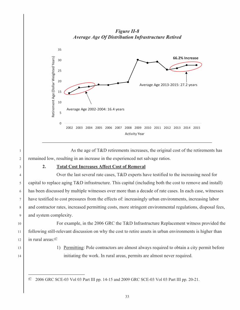
33

Figure II-8 Average Age Of Distribution Infrastructure Retired

As the age of T&D retirements increases, the original cost of the retirements has 1

remained low, resulting in an increase in the experienced net salvage ratios. 2

2. Total Cost Increases Affect Cost of Removal 3

Over the last several rate cases, T&D experts have testified to the increasing need for 4

capital to replace aging T&D infrastructure. This capital (including both the cost to remove and install) 5

has been discussed by multiple witnesses over more than a decade of rate cases. In each case, witnesses 6

have testified to cost pressures from the effects of: increasingly urban environments, increasing labor 7

and contractor rates, increased permitting costs, more stringent environmental regulations, disposal fees, 8

and system complexity. 9

For example, in the 2006 GRC the T&D Infrastructure Replacement witness provided the 10

following still-relevant discussion on why the cost to retire assets in urban environments is higher than 11

in rural areas:47 12

1) Permitting: Pole contractors are almost always required to obtain a city permit before 13

initiating the work. In rural areas, permits are almost never required. 14

47 2006 GRC SCE-03 Vol 03 Part III pp. 14-15 and 2009 GRC SCE-03 Vol 03 Part III pp. 20-21.

0

5

10

15

20

25

30

35

2002 2003 2004 2005 2006 2007 2008 2009 2010 2011 2012 2013 2014 2015

Retirem

entA

ge(DollarW

eightedYears)

Activity Year

Average Age 2002 2004: 16.4 years

Average Age 2013 2015: 27.2 years

66.2% Increase

34

2) Accessibility: Urban areas are frequently inaccessible by trucks and require that a 1

crane be rented or that the pole be carried into the back yard and set manually. Rural 2

areas are typically truck-accessible. 3

3) Congestion: Higher customers per circuit in urban areas contribute to higher 4

congestion per pole than in rural areas. For example, an urban pole can be expected to 5

be taller, as well as have more conductors, transformers, and cross-arms than a rural 6

pole. In addition, the work may be performed on energized lines requiring specially 7

trained crews and safety requirements. 8

4) Repairs: Urban areas frequently require that repairs are made to the concrete 9

sidewalks, a requirement not typically necessary in rural areas. 10

Los Angeles County’s population experienced significant growth48 in the post-World 11

War II period through the 1970s. This post-war population growth has increased the level of 12

urbanization across SCE’s service territory, putting upward pressure on costs. As a result of this, when 13

assets originally installed in a rural environment are removed, the net salvage ratio reflects a very low 14

original install cost for these assets. But these same assets are likely being replaced in a now more urban 15

environment, adding to the upward pressure on removal cost. This experience can have a significant 16

effect on the net salvage ratios—lower original cost (denominator) and higher cost of removal 17

(numerator). 18

Given the increasing age of this infrastructure and the increasing urbanization associated 19

with the post-war population growth, increases in the realized net salvage ratios is not surprising. As a 20

result, however, the conditions present in SCE’s service territory over this period of time may not be a 21

realistic expectation of the future. In this case, and as further discussed immediately below, a per-unit 22

analysis controls for this variation, and better represents SCE’s expectation about the future levels of net 23

salvage. 24

3. SCE’s Per-Unit Analysis is Indifferent to the Realized Net Salvage Ratios 25

As described in Section B.1 of Chapter II, a per-unit analysis takes a different approach 26

than Standard Practice U-4 in analyzing the expected levels of future net salvage. Rather than reviewing 27

the relationship between historical costs of assets and the net salvage experienced in the past, the per-28

unit analysis uses the recorded average cost to retire each unit of property, and then applies per-unit 29

48 2009 GRC SCE-03 Vol 03 Part 3 p. 15 (SCE Territory – Population and System Demand).

35

costs to existing plant balances to forecast future net salvage given the anticipated timing of retirements. 1

This approach to estimating future net salvage helps ensure that the results of the analysis are applicable 2

to the mixture of plant that is serving customers today. Over time, as this mix of plant balances change, 3

SCE will have the opportunity to reflect these changes in future per-unit analyses presented in its rate 4

cases. 5

36

III. 1

DEPRECIATION STUDY 2

Chapter II, above, explained how SCE complied with the Commission’s compliance directives 3

and addressed the difference between traditional and per-unit analyses. The depreciation study 4

addressing T&D assets, presented in Section A in Q&A format, was undertaken by an external 5

consultant, Ronald E. White Ph.D. of Foster Associates Consultants, LLC. Dr. White provided SCE with 6

life and net salvage parameters that SCE then used to calculate the proposed depreciation rates. SCE 7

also conducted an in-house depreciation study of its Generation and G&I depreciable plant assets, 8

discussed by an in-house SCE expert witness in Section B, below. 9

Unlike the Simulated Plant Record (SPR) procedure used in prior SCE rate cases, Dr. White 10

performed an actuarial service life analysis using aged data from 2002 to 2015. In the 2012 GRC, the 11

Commission stated that aged data is likely to be more reliable than SPR data, and it ordered SCE to 12

“inform the Commission whether it used any aged data, and if not, when sufficient data is expected to be 13

available.”49 In its 2015 GRC testimony, SCE stated that it began collecting aged data in 2008 and that it 14

did not have sufficient aged data to perform an effective actuarial life analysis for the 2015 GRC.50 This 15

statement was based on an incorrect assumption that the Company began collecting aged data in 2008 16

when it implemented PowerPlan as its capital system of record.51 In preparing its showing for this 17

proceeding, SCE discovered that PowerPlan contains reconciled aged plant activity from 2002 forward. 18

Thus, for this GRC, Foster Associates LLC performed an actuarial life analysis using the aged data from 19

2002 to 2015.52 20

Section A of Chapter III, below, which is in Q&A format, is the direct testimony of Dr. Ronald 21

E. White of Foster Associates LLC. 22

49 D.12-11-051 p. 685. 50 See Testimony in 2015 GRC, SCE-10, Vol. 02, Revision 1A, p. 33. SCE stated that it expected that aged data

may become useful “in 10 years or so.” Id. 51 PowerPlan was used only as the depreciation system of record prior to 2008. 52 SCE possesses some aged retirement data from 1994 through 2001 in Excel format outside of SCE’s current

capital system of record (PowerPlan). Neither SCE nor its outside expert evaluated or relied on the aged data in the 1994-2001 Excel sheets.

37

A. T&D - Average Service Life and Net Salvage Proposals 1

1. Development of Depreciation Rates 2

Q. PLEASE EXPLAIN WHY DEPRECIATION STUDIES ARE NEEDED FOR 3

ACCOUNTING AND RATEMAKING PURPOSES. 4

A. The goal of depreciation accounting is to charge to operations a reasonable estimate of the cost 5

of the service potential of an asset (or group of assets) consumed during an accounting interval.53 6

A number of depreciation systems have been developed to achieve this objective, most of which 7

employ time as the apportionment base. 8

Implementation of a time–based (or age–life) system of depreciation accounting requires the 9

estimation of several parameters or statistics related to a plant account. The average service life 10

of a vintage, for example, is a statistic that will not be known with certainty until all units from 11

the original placement have been retired from service. A vintage average service life, therefore, 12

must be estimated initially and periodically revised as indications of the eventual average service 13

life becomes more certain. Future net salvage rates and projection curves, which describe the 14

expected distribution of retirements over time, are also estimated parameters of a depreciation 15

system that are subject to future revisions. Depreciation studies should be conducted periodically 16

to assess the continuing reasonableness of parameters and accrual rates derived from prior 17

estimates. 18

The need for periodic depreciation studies is also a derivative of the ratemaking process 19

which establishes prices for utility services based on costs. Absent regulation, deficient or 20

excessive depreciation rates will produce no adverse consequence other than a systematic over or 21

understatement of the accounting measurement of earnings. While a continuance of such 22

practices may not comport with the goals of depreciation accounting, the achievement of capital 23

recovery is not dependent upon either the amount or the timing of depreciation expense for an 24

unregulated firm. In the case of a regulated utility, however, recovery of investor–supplied 25

capital is dependent upon allowed revenues, which are in turn dependent upon approved levels of 26

depreciation expense. Periodic reviews of depreciation rates are, therefore, essential to the 27

53 The service potential of an asset is the present value of future net revenue (i.e., revenue less expenses

exclusive of depreciation and other non–cash expenses) or cash inflows attributable to the use of that asset alone.

38

achievement of timely capital recovery for a regulated utility. 1

It is also important to recognize that revenue associated with depreciation is a significant 2

source of internally generated funds used to finance plant replacements and new capacity 3

additions. This is not to suggest that internal cash generation should be substituted for the goals 4

of depreciation accounting. However, the potential for realizing a reduction in the marginal cost 5

of external financing provides an added incentive for conducting periodic depreciation studies 6

and adopting proper depreciation rates. 7

Q. PLEASE DESCRIBE THE PRINCIPAL STEPS INVOLVED IN 8

CONDUCTING A DEPRECIATION STUDY. 9

A. The first step in conducting a depreciation study is the collection of plant accounting data needed 10

to conduct a statistical analysis of past retirement experience. Data are also collected to permit an 11

analysis of the relationship between retirements and realized gross salvage and cost of removal. 12

The data collection phase should include a verification of the accuracy of the plant accounting 13

records and a reconciliation of the assembled data to the official plant records of the Company. 14

The next step in a depreciation study is the estimation of service life statistics from an 15

analysis of past retirement experience. The term life analysis is used to describe the activities 16

undertaken in this step to obtain a mathematical description of the forces of retirement acting 17

upon a plant category. The mathematical expressions used to describe these forces are known as 18

survival functions or survivor curves. 19

Life indications obtained from an analysis of past retirement experience are blended with 20

expectations about the future to obtain an appropriate projection life curve. This step, called life 21

estimation, is concerned with predicting the expected remaining life of property units still 22

exposed to the forces of retirement. The amount of weight given to the analysis of historical data 23

will depend upon the extent to which past retirement experience is considered descriptive of the 24

future. 25

Average and future net salvage rates are ideally estimated from a historical analysis of the 26

cost per unit to install and the net cost per unit to retire major retirement units. A per unit 27

analysis explicitly recognizes that the cost per unit to retire an asset is independent of the age of 28

the asset when it is retired from service. The cost to retire a foot of conductor today, for example, 29

is no different for a conductor that was installed yesterday or a conductor that was installed many 30

years ago. As a result, percentage rate required to accrue for $5 per foot of removal expense on a 31

39

conductor costing $10 per foot to install is twice the rate required to accrue the same amount of 1

removal expense on a conductor costing $20 per foot to install. 2

Although a per unit analysis of installation and retirement costs is the most desirable 3

treatment of net salvage, time and cost considerations (as well as the availability of the required 4

data) often dictate a less rigorous analysis. Net salvage rates are frequently developed from a 5

historical analysis using a three to ten–year moving average of the ratio of realized salvage and 6

cost of removal to associated retirements. Net salvage estimates are also obtained from 7

engineering studies of the cost to dismantle or abandon existing facilities. 8

2. 2016 Service–Life Study 9

Q. DID SCE PROVIDE FOSTER ASSOCIATES PLANT ACCOUNTING DATA 10

FOR ESTIMATING SERVICE LIFE PARAMETERS? 11

A. Yes. Service life statistics estimated in the 2016 study were derived from plant accounting 12

transactions recorded over the period 2002 through 2015. Detailed accounting transactions were 13

extracted from the Continuing Property Record (CPR) system and assigned transaction codes 14

which describe the nature of the accounting activity. Transaction codes for plant additions, for 15

example, were used to distinguish normal additions from acquisitions, purchases, 16

reimbursements and adjustments. Similar transaction codes were used to distinguish normal 17

retirements from sales, reimbursements, abnormal retirements and adjustments. Transaction 18

codes were also assigned to transfers, capital leases, gross salvage, cost of removal and other 19

accounting activity that should be considered in a depreciation study. 20

The accuracy and completeness of the assembled database was verified for activity years 21

2002 through 2015 by comparing the beginning plant balance, additions, retirements, transfers 22

and adjustments, and the ending plant balance derived for each activity year to the official plant 23

records of the Company. Age distributions of surviving plant at December 31, 2015 were 24

reconciled to the CPR. 25

Q. HOW WERE SERVICE–LIFE ESTIMATES DERIVED FOR SCE PLANT 26

AND EQUIPMENT? 27

A. As noted above, the first step in estimating service lives is called life analysis. All transmission, 28

distribution and general depreciable plant accounts were analyzed using a technique in which 29

first, second and third degree polynomials were fitted to a set of observed retirement ratios. The 30

40

resulting function was expressed as a survivorship function, which was numerically integrated to 1

obtain an estimate of the average service life. The smoothed survivorship function was then 2

fitted by a weighted least–squares procedure to the Iowa–curve family to obtain a mathematical 3

description or classification of the dispersion characteristics of the data. Service life indications 4

derived from the statistical analyses were blended with informed judgment and expectations 5

about the future to obtain an appropriate projection life curve for each plant category. The 6

analysis of each plant account is contained in Appendix A. 7

Q. PLEASE EXPLAIN IN GREATER DETAIL HOW LIFE ANALYSES WERE 8

CONDUCTED IN THE 2016 STUDY. 9

A. The fundamental probability distribution of interest in estimating the service life of industrial 10

property is called a hazard function. This function, which is also used in reliability theory, is an 11

equation that describes the conditional probability of retirement (called a hazard rate) during an 12

age interval given survival to the beginning of the interval. So, for example, the probability that 13

plant that has been in service, say for 5 years, will be retired during the 6th year is a conditional 14

probability of retirement. In other words, the probability is conditioned upon having achieved an 15

age of 5 years. 16

Graduating or smoothing observed hazard rates is an application of inferential statistics 17

which draws inferences and predictions about a population based on samples of data taken from 18

the population of interest. Projection lives and projection curves are population parameters 19

“inferred” from a statistical analysis of the underlying forces of retirement described by 20

probability distributions. 21

The object of a statistical analysis of plant retirements is to find the form of an equation that 22

best describes the conditional probabilities of retirement, where the form of the equation is 23

driven by the underlying forces of retirement. Any number of equations can be considered as 24

candidates for selection. The so–called Iowa curves are a family of distributions most often used 25

in conducting depreciation studies. 26

Each Iowa curve has a unique hazard function derived from the ratio of its retirement 27

frequency distribution to its survivor distribution. Unfortunately, however, Iowa hazard functions 28

cannot be written as explicit equations. It is for this reason that polynomials of the form 29

2 3y a bx cx dx are used to estimate hazard functions. The variable y is the hazard rate 30

41

and x is the age interval of the rate.54 A polynomial can be transformed into a survivor function 1

and plotted against an Iowa curve to visually observe the derived survivor curve expressed as an 2

Iowa curve. 3

The problem, therefore, is to estimate the coefficients (i.e., a, b, c and d) of the polynomial 4

from an estimate of hazard rates derived from a sampling of historical retirements recorded for a 5

plant category. Different estimators of the hazard rate can be used depending upon the desired 6

statistical properties of the estimator. The ratio of retirements to exposures is most often used for 7

depreciation studies. 8

Coefficients were estimated in the 2016 study using Orthogonal Polynomials. An orthogonal 9

polynomial is not a special form of a polynomial. It is a procedure developed by Tchebysheff to 10

estimate the coefficients of a polynomial (using regression) without rewriting the normal 11

equations for each successive power of the polynomial. The coefficients of a second degree 12

equation, for example, can be derived from a first degree equation without rewriting the 13

equations used in a normal least squares regression. 14

Coefficients and polynomials were estimated for numerous trials or samples of retirements 15

recorded over various bands of activity years. An activity year is the calendar year in which 16

retirements were recorded. Retirements from vintages of like ages are combined to increase the 17

size of the samples from which hazard rates are estimated. The motivation for examining various 18

bands of activity years is to observe service–life trends to the extent they may be detectable. 19

Each polynomial was transformed or converted to a survivor function (or survivor curve 20

when plotted) from which an estimate of the projection life was derived. The polynomial form of 21

the hazard functions were also plotted and visually inspected as an aid to better understanding 22

the forces of retirement acting upon a plant category. 23

Polynomials transformed to survivor functions were then fitted to Iowa–type curves with 24

projection lives set equal to those derived from the polynomials. The purpose of fitting to Iowa 25

curves is to obtain service–life descriptors more familiar to users of Iowa curves. It would be 26

more obscure and less informative to describe survivor curves by the coefficients of a 27

polynomial. 28

54 The reason polynomials are limited to a third degree term (i.e., a polynomial having an 3x term) is that some

low modal Iowa curves exhibit two inflection points in a plot of the hazard function.

42

Q. WERE FACTORS OTHER THAN SERVICE–LIFE INDICATIONS DERIVED 1

FROM THE STATISTICAL STUDIES CONSIDERED IN ESTIMATING 2

SERVICE–LIVES FOR SCE? 3

A. Yes. As discussed earlier, estimating service lives is a two–step procedure. The first step (life 4

analysis) is largely mechanical and primarily concerned with history. Statistical techniques are 5

used in this step to obtain a mathematical description of past forces of retirement acting upon a 6

plant category and an estimate of the projection life implied from observed historical experience. 7

The second step (life estimation) is concerned with predicting the expected remaining life of 8

property units still exposed to forces of retirement and the service life of future plant additions. It 9

is a process of blending the results of a life analysis with information (mostly qualitative) and 10

informed judgment to obtain an appropriate projection life and curve descriptive of future 11

expectations. The amount of weight given to a life analysis will depend upon the extent to which 12

past retirement experience is considered descriptive of the future. Both life analysis and life 13

estimation require an understanding of the limitations of statistical studies and the need for 14

reasonable and informed judgment. 15

Q. ARE FACTORS YOU CONSIDERED IN LIFE ESTIMATION DESCRIBED 16

IN THE 2016 STUDY? 17

A. Yes. Appendix A contains a narrative explanation of both quantifiable factors (life analyses) and 18

non–quantifiable factors (largely life estimation) considered by Foster Associates in 19

recommending appropriate projection lives and curves for SCE. In those instances in which 20

statistical indications could not be derived and/or observed indications were adjusted for 21

operational, financial or ratemaking reasons, Foster Associates deferred to SCE in the selection 22

of appropriate service lives. 23

Q. IS A PROJECTION LIFE THE SAME AS AN AVERAGE SERVICE LIFE? 24

A. No. A projection life is an estimate of the mean service–life of the population from which 25

retirements are a random sample. The average service life of a plant category is a function of the 26

age distribution of surviving plant (i.e., plant currently in service by vintage–year of installation) 27

and a selected level of asset grouping such as broad–group, vintage–group or equal-life group. If 28

retirements are distributed over varying ages, the broad–group procedure (which assumes that 29

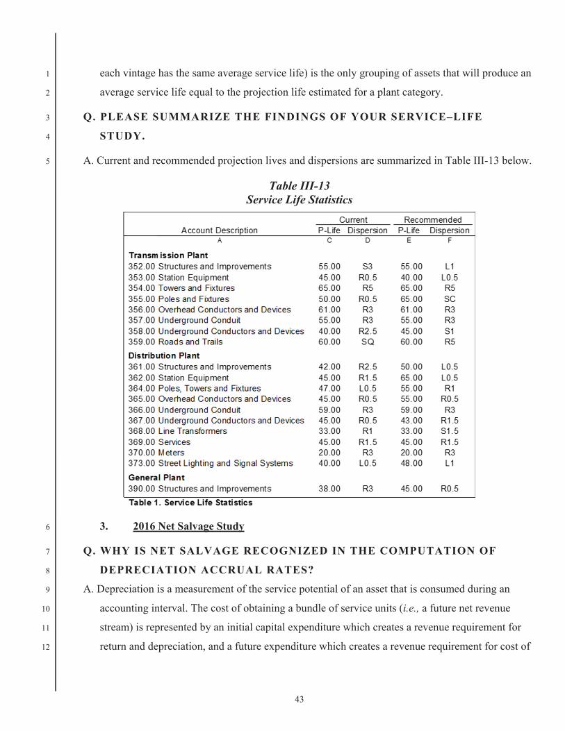
43

each vintage has the same average service life) is the only grouping of assets that will produce an 1

average service life equal to the projection life estimated for a plant category. 2

Q. PLEASE SUMMARIZE THE FINDINGS OF YOUR SERVICE–LIFE 3

STUDY. 4

A. Current and recommended projection lives and dispersions are summarized in Table III-13 below. 5

Table III-13 Service Life Statistics

3. 2016 Net Salvage Study 6

Q. WHY IS NET SALVAGE RECOGNIZED IN THE COMPUTATION OF 7

DEPRECIATION ACCRUAL RATES? 8

A. Depreciation is a measurement of the service potential of an asset that is consumed during an 9

accounting interval. The cost of obtaining a bundle of service units (i.e., a future net revenue 10

stream) is represented by an initial capital expenditure which creates a revenue requirement for 11

return and depreciation, and a future expenditure which creates a revenue requirement for cost of 12

44

removal reduced by salvage proceeds. The matching principle of accounting provides that both 1

the initial and future expenditures should be allocated to the accounting periods in which the 2

service potential of an asset is consumed. The standard or criterion that should be used to 3

determine a proper net salvage rate is, therefore, cost allocation over economic life in proportion 4

to the consumption of service potential. If some other standard (such as cash flow or revenue 5

requirements) is considered more important in setting depreciation rates, then cost allocation 6

theory must be abandoned as the foundation for depreciation accounting. 7

The need to include net salvage in the development of depreciation rates is widely recognized 8

and accepted by a substantial majority of state regulatory commissions as a standard ratemaking 9

principle. The FERC Uniform System of Accounts (USoA), for example, describes depreciation 10

as the “… loss in service value” where service value is defined as “… the difference between 11

original cost and net salvage value of gas plant.” Net salvage value means “the salvage value of 12

property retired less the cost of removal.” 13

The economic principle underlying both the accounting and ratemaking treatment of net 14

salvage is that in addition to return of and return on invested capital and taxes, a revenue 15

requirement for removal expense (or a reduction in the revenue requirement attributable to gross 16

salvage) is created when an asset is placed in service. It is customary and appropriate for 17

regulated utilities, therefore, to include a net salvage component in its depreciation rates to more 18

nearly achieve the goals of depreciation accounting and to equitably distribute the revenue 19

requirement for removal expense over the period in which the assets that created the requirement 20

are used to provide utility service. 21

Q. WHAT IS A FUTURE NET SALVAGE RATE? 22

A. Future net salvage (in percent) is the sum of future net salvage (i.e., gross salvage less cost of 23

removal) at a given observation age divided by the surviving plant investment at that age. 24

Q. WHAT IS AN AVERAGE NET SALVAGE RATE? 25

A. Average net salvage (in percent) is the sum of realized and future net salvage divided by the 26

plant investment at age zero. Stated differently, average net salvage is the total estimated salvage 27

less cost of removal for a vintage (or group of vintages) expressed as a percent of the original 28

vintage additions. Future net salvage is related to the surviving plant of a vintage (or group of 29

vintages) whereas average net salvage is associated with the original vintage addition. 30

45

Q. ARE YOU FAMILIAR WITH THE COMMISSION’S DECISION IN SCE’S 1

2015 GRC (D.15-11-021) REGARDING NET SALVAGE PROPOSALS? 2

A. Yes. In the 2015 GRC Decision, the Commission directed SCE to provide more detail in support 3

of its net salvage proposals for at least five of the largest accounts, as measured by proposed 4

annual depreciation expense. At a minimum, this detail shall include: 5

1. “A quantitative discussion of historical and anticipated future Cost of Removal 6 (COR) on a per unit basis for the large (greater than 15% as measured by the 7 portion of plant balance) asset classes in the account. This discussion should 8 identify and explain the key factors in changing or maintaining the per–unit 9 COR.” 10

2. “A quantitative discussion of historical and anticipated future retirement mix 11 (i.e., retirements among different asset classes), identifying and explaining the 12 key factors in changing or maintaining this mix.” 13

3. “A quantitative discussion of the life of assets and original cost of assets being 14 retired, in relation to the COR, on both a historical and anticipated future basis. 15 This discussion should be integrated with and/or cross–reference the proposal 16 for life characteristics.” 17

4. “An account–specific discussion of the process for allocating costs to COR.”55 18

a) Directive No. 1 19

Q. WERE HISTORICAL AND FUTURE NET SALVAGE COSTS DERIVED ON 20

A PER UNIT BASIS IN COMPLIANCE WITH THE COMMISSION’S FIRST 21

DIRECTIVE? 22

A. Yes. Per unit net salvage analyses were conducted for the nine (9) plant accounts listed in Table 23

III-14, below. 24

55 D.15-11-021, pp. 554-555.

46

Table III-14 Per Unit Net Salvage Accounts

Each of the nine plant accounts was grouped into one or more subpopulations of major 1

equipment categories. Historical per unit ratios (defined as net cost per unit to retire divided by 2

the cost per unit to install) were used in both the historical and future per unit analyses. Net costs 3

to retire (or net salvage) were used in the analysis to maintain consistency with future net salvage 4

parameters used in the formulation of remaining–life accrual rates. Gross salvage is generally 5

small in relation to cost of removal. 6

Historical per unit ratios were examined and compared with the ratio of realized net salvage 7

to the associated retirements. In most instances, the ratio of net salvage to retirements is greater 8

than historical per unit ratios observed over the period 2009–2014. This is predictable since net 9

savage is recorded in current dollars and retirements are recorded in historical dollars. 10

Future per unit ratios were derived using a weighted average of the subpopulation net salvage 11

per unit values recorded over the period 2009–2015. These values appear in the numerator of 12

future per unit ratios. This treatment was decided after multiple meetings and discussions with 13

SCE engineers and subject matter experts who reported that SCE has no planned or expected 14

changes in retirement activities that would measurably change average net salvage per unit 15

values recorded in recent activity years. Other than recognizing future inflation, historical net 16

salvage per unit values were therefore retained in the forecast of future net salvage rates. 17

Subpopulations and average historical per unit net salvage costs are summarized in Table III-15 18

below. 19

47

Table III-15 Average Net Salvage Per Unit to Retire

The per unit cost of plant additions used in forecasting future net salvage rates was obtained 1

by dividing vintaged plant in service at December 31, 2015 (i.e., age distributions of surviving 2

plant) by vintaged units in service within each subpopulation. The ratio of average net salvage 3

per unit experienced over the period 2009–2015 (adjusted for inflation) to the per unit cost of 4

plant in service is the ratio that was applied to forecasted retirements to estimate future net 5

48

salvage for each vintage. The sum of future net salvage over all vintages divided by current plant 1

account balances produces an estimated future net salvage rate for each primary account. The 2

formulation of per unit net salvage rates is contained in Appendix B. 3

Q. PLEASE SUMMARIZE THE FINDINGS OF YOUR PER UNIT NET 4

SALVAGE ANALYSIS. 5

A. Future net salvage rates derived with inflation rates ranging between zero (0) and three (3) 6

percent are summarized in below. 7

Table III-16 Future Net Salvage Rates

Q. HOW WERE NET SALVAGE RATES ESTIMATED FOR ACCOUNTS NOT 8

INCLUDED IN THE PER UNIT NET SALVAGE ANALYSIS? 9

A. A five–year moving average analysis of the ratio of realized salvage and removal expense to the 10

associated retirements was used to: a) estimate a realized net salvage rate; b) detect the 11

emergence of historical trends; and c) establish a basis for estimating a future net salvage rate. 12

Cost of removal and salvage opinions obtained from Company personnel were blended with 13

judgment and historical net salvage indications in developing estimates of the future. The 14

analysis of net salvage is contained in Appendix A. 15

Although future per unit ratios applied to a forecast of future retirements provides a more 16

rigorous estimate of future net salvage rates, it is the opinion of Foster Associates that the ratio of 17

realized net salvage to retirements provides reasonable estimates of future net salvage rates to the 18

extent that future inflation is similar to the past. Estimating depreciation rates, however, is not an 19

exact science; errors of estimate in both service lives and nets salvage rates will always remain. 20

49

b) Directive No. 2 1

Q. WERE HISTORICAL AND FUTURE RETIREMENT MIXES EVALUATED 2

IN COMPLIANCE WITH THE COMMISSION’S SECOND DIRECTIVE? 3

A. Yes. As noted above, each of the nine plant accounts was divided into one or more 4

subpopulations of major equipment categories. The mix of equipment classified in each 5

subpopulation and the size of each subpopulation as a percent of the current investment in each 6

related plant account were reviewed by SCE engineering and plant accounting personnel. No key 7

factors were identified from this review that would suggest the future retirement mix or relative 8

size of each subpopulation will be significantly different from the current composition and 9

grouping of subpopulations. 10

c) Directive No. 3 11

Q. WERE RECOMMENDED LIFE CHARACTERISTICS AND NET COST OF 12

REMOVAL INTEGRATED IN COMPLIANCE WITH THE COMMISSION’S 13

THIRD DIRECTIVE? 14

A. Yes. The directive to provide a quantitative discussion of asset life and original cost of assets 15

being retired, in relation to the COR on a historical basis, was interpreted to mean an 16

examination of the average age of retirements associated with the recording of COR. Work 17

papers supporting Appendix A provide a summary (Schedule E) of the average age of 18

retirements and recorded COR for each of the per unit accounts. Although net salvage is often 19

recorded subsequent to the recording of retirements, it can be observed that COR as a percent of 20

retirements is a function of the age of retirements and generally increases with increases in the 21

average age. 22

As noted earlier, a prospective per–unit analysis should be designed to produce estimates of 23

future net salvage rates respecting the principle that the net cost per unit to retire an asset in 24

independent of the age of the asset when it is retired from service. The percentage rate applied to 25

the cost of an old asset to accrue the same cost per unit to retire a newer asset, however, depends 26

upon the relative difference in the cost per unit incurred to install the assets. Integration of per 27

unit ratios with life characteristics necessitates forecasting vintaged retirements using projection 28

lives and curves estimated for each plant account. 29

Estimates of the amount and timing of future net salvage were derived from an application of 30

50

the ratio of per unit net costs to retire and per unit installed costs of each vintage within a 1

subpopulation, to future retirements (forecasted by vintage) using the projection lives and curves 2

estimated in the statistical life studies. Inflation rates ranging between zero and three percent 3

were employed in the analysis to recognize the likelihood of increasing net salvage solely 4

attributable to inflation. 5

Other than a range of assumed inflation rates and parameters estimated in the service–life 6

studies, no elements of qualitative judgment were required or exercised in estimating future net 7

salvage rates from the per unit analysis. 8

d) Directive No. 4 9

Q. THE COMMISSION’S FOURTH DIRECTIVE IN APPLICATION A.13–11–10

003 WAS TO PROVIDE AN ACCOUNT–SPECIFIC DISCUSSION OF THE 11

PROCESS FOR ALLOCATING COSTS TO COR. HAS SCE COMPLIED 12

WITH THIS DIRECTIVE? 13

A. Yes. The process for allocating costs is described in the direct testimony of SCE witness Alan 14

Varvis in this Exhibit. 15

Q. DOES THIS CONCLUDE YOUR DIRECT TESTIMONY? 16

A. Yes, it does.17

51

B. Generation and G&I - Average Service Life and Net Salvage Proposals 1

1. Purpose and Scope 2

This chapter covers the average service lives and net salvage proposals for SCE’s 3

Generation and General & Intangible (G&I) assets. For G&I assets, SCE proposes to retain the same 4

service lives and net salvage rates as authorized in the 2015 GRC Decision. 5

2. Generation-Related Property 6

a) Average Service Lives for Generation Assets 7

Generating facilities are life span assets that consist of large plant assets expected 8

to retire all at one time, with some smaller components retiring earlier during the service life of the plant 9

(called “interim retirements”). To determine the average life of the plant asset, SCE adjusts the life span 10

downward to take into account the shorter-lived interim retirements. The life span for a generating 11

facility as a whole depends on the factors affecting the final shutdown: operating license, fuel and 12

resource availability, contractual obligations, the relative efficiency of the generating units, and so forth. 13

The total life span is determined largely as an engineering judgment based on the factors previously 14

mentioned. 15

Interim retirements consist of such items as pumps, motors, and other individual 16

generating components that retire depending on the factors specifically affecting them—wear and tear, 17

reliability, obsolescence, and so forth. The impacts of the life span and the interim retirements on the 18

overall average service life of the plant asset are determined separately. SCE considered the interim 19

retirement adjustment first by estimating the future level of annual interim retirements as a percent of the 20

plant balance (i.e., an interim retirement rate or IR rate). The estimate of an IR rate is made by analyzing 21

the historical levels of interim retirements. The determined annual IR rate is applied to the current plant 22

balance over the remaining life of the plant to determine the necessary adjustment to the overall 23

remaining life of the generating station. For example, if a generating plant has a 10-year remaining life 24

and an IR rate of 1.4 percent per year, then about 14 percent of the current plant balance would retire as 25

interim retirements (10 years times 1.4 percent year) and the remaining 86 percent would retire as a final 26

retirement. The resulting survivor curve is shown in Figure III-9. 27

52

Figure III-9 Life Span Survivor Curve*

* Remaining Life Span = 10 years; IR Rate = 1.4%.

As Figure III-10 demonstrates, the average life is equal to the life span adjusted 1

for the shorter life of the interim retirements. The remaining life adjustment is calculated as follows: 2

Figure III-10 Life Span: Remaining Life Adjustment

Table III-17 summarizes SCE’s proposed generation average service lives as 3

compared to those authorized in the 2015 GRC. What follows is a plant-by-plant discussion of the 4

proposed average service lives. 5

0%

20%

40%

60%

80%

100%

0 1 2 3 4 5 6 7 8 9 10Years

Avg. Life = Rem. Life IR Adjustment9.3 yrs = 10 yrs 0.7 yrs

% Surviving

IR Adjustment

Remaining Life Rem. Life Span x IR Rate Rem. LifeAdjustment 2 Span

10 Years x 1.4%2

= x

0.7 Years 10 Yearsx=

53

Table III-17 Generation Service Life Spans

(1) Palo Verde Nuclear Generating Station (PVNGS) 1

The Nuclear Regulatory Committee (NRC) licenses for PVNGS Units 1, 2

2, and 3 end June 1, 2045, April 24, 2046, and November 25, 2047, respectively, resulting in an average 3

30.5 year remaining life span for the station as of December 31, 2015. In addition, recent retirement 4

activity supports adjusting the average remaining life down by 2.5 years to 28 years to account for the 5

effect of interim retirements. 6

(2) Hydro Generation 7

SCE’s hydro generation system consists of 76 generating units and 8

associated facilities accounted for in 60 different accounting locations. Nearly all of SCE’s hydro 9

facilities (99 percent) is covered by FERC licenses. The licenses have a variety of termination dates—10

from expired (either in the process of being relicensed or decommissioned) to 2046. The total life span 11

of SCE’s current license periods for those plants without expired licenses range between 5 and 30 years. 12

Recently, FERC has issued renewals with license periods averaging 40 years. 13

Prior license renewal does not guarantee that the generating plant will last 14

indefinitely. There are no guarantees that the FERC will continue to grant the company licenses or that 15

the generating units will continue to be economic. Moreover, the individual components making up a 16

generating station will continue to wear out, be retired, and need to be replaced. Consequently, SCE 17

proposes that the hydro generation plant be depreciated over the remaining life spans associated with the 18

Life SpansGeneration Facility Authorized Proposed

A B CNuclear Production Palo Verde 30.5 yrs 28.0 yrsHydro Production 26 yrs 19.9 yrsOther ProductionPebbly Beach 45 yrs 25 yrsMountainview 35 yrs 35 yrsPeakers 35 yrs 35 yrsSolar Photovoltaic 25 yrs 20 yrsFuel Cells 10 yrs 10 yrsEnergy Storage N/A 10 yrs

54

individual FERC licenses.56 For generating stations with already expired, or within five years of license 1

termination, SCE proposes that the life spans be extended by the estimated license life in its current 2

FERC license applications.57 3

(3) Pebbly Beach 4

The Pebbly Beach generating station consists of six diesel generating 5

units, ranging in capacity from 1.0 MW to 2.8 MW. In its last GRC, SCE was authorized a 45-year 6

average service life for this account on the basis that each of the six units would experience increasing 7

risk of obsolescence and failure after two overhaul cycles (approximately 22 years between overhauls). 8

Because of the difficulty in sourcing alternative supply of generation for Catalina Island, SCE engineers 9

expect these units to remain in-service for the foreseeable future. However, to help ensure continued 10

operations, SCE engineers state that the units require a zero-time overhaul58 after approximately 100 to 11

120 thousand operating hours. Based on SCE’s actual experience with the operations of these units, the 12

time between overhauls is approximately 25 years. 13

For example, the SCE is proposing to reduce the average service life for 14

this account from the currently authorized 45 years to 25 years. This change is concurrent with moving 15

the start of the amortization period from the vintage year to the date of the last overhaul. This 25-year 16

life allows SCE to recover the cost of each zero-time overhaul over its useful life with little impact to the 17

remaining life as shown in Table III-18 below. 18

56 In the case of the 1 percent of hydro plant not covered by a FERC license, SCE applies the average life

determined for the plant that is covered by FERC license. 57 The average application license period is 44 years. The exception to this life span extension is the

amortization period for the hydro relicensing costs. These relicensing costs are only amortized over the associated license period for which they were spent.

58 A zero-time overhaul restores operations of the unit to like-new operating conditions.

55

Table III-18 59 Comparison of SCE’s 2015 Authorized and 2018 Proposed Lives for

Pebbly Beach Generating Station

There have been insufficient interim retirements to estimate an IR rate for 1

this plant; consequently both the remaining life span and the average remaining life are 15.5 years for 2

this account. 3

(4) Mountainview 4

SCE is proposing to retain Mountainview’s currently authorized 35-year 5

life span as established in the 2015 GRC Decision. There have been insufficient interim retirements to 6

estimate an IR rate for this plant; consequently both the remaining life span and the average remaining 7

life are 25 years for this account. 8

(5) Peakers 9

SCE is proposing to retain the currently authorized 35-year average 10

service life for Peaker. There have been insufficient interim retirements to estimate an IR rate for this 11

plant; consequently both the remaining life span and the average remaining life are 28 years for this 12

account. 13

(6) Solar Photovoltaic 14

The currently authorized average service life for Solar Photovoltaic (PV) 15

equipment is 25 years. SCE is proposing to return to the previously authorized 20-year average service 16

life. Based on discussions with SCE engineers60 the major components of this account will have 17

significantly shorter service lives than the currently authorized 25-year life. Engineers indicate that the 18

59 Refer to WP SCE-09 Vol. 03, Book A, p. 203 (Generation Life Spans). 60 Refer to WP SCE-09 Vol. 03, Book A, p. 204 (Generation Life Spans).

Line 2015 GRC 2018 GRCNo. Item Authorized Proposed1. Average Start Date 1986 20062. Proposed ASL 45 25

3. = 1.+2. Estimated Ret. Date 2031 20314. = 3. - 2015 Rem. Life a/o 1/1/2016 15.7 15.5

56

equipment in this account is expected to fail significantly sooner than the currently authorized 25-year 1

authorized life. For example, the three main components61 include: 2

Solar Panels – 10-12 years 3

Inverters – 5-8 years (warrantied for 5 years) 4

Control System – 6-8 years for obsolescence to set in. 5

In addition, the rooftop leases granting SCE the rights to use the rooftop 6

facilities is currently 20-years. Given the uncertainty of lease renewal and short expectations about the 7

life of the equipment, a 20-year life proposal is reasonable for this account. There have been insufficient 8

interim retirements to estimate an IR rate for this plant; consequently both the remaining life span and 9

the average remaining life are 16 years for this account. 10

(7) Fuel Cells 11

SCE owns and operates two fuel cell demonstration facilities. The plants, 12

located at California State University, San Bernardino (CSUSB) and University of California Santa 13

Barbara (UCSB) were installed in September 2012 and October 2013 respectively. SCE is proposing to 14

retain the currently authorized 10-year average service life. This proposal is consistent with our 15

expectations that title to the demonstration facilities will be transferred to the site owners at the end of 16

their 10-year lease. 17

(8) Energy Storage 18

The Commission has required SCE to procure and install 580 MW of 19

energy storage facilities in its service territory by 2020. These facilities represent emerging technology 20

and face significant risk of technological obsolescence in the future. SCE estimates the life of Energy 21

Storage by the design life, cycle times of the proposed facilities, discussion with engineers, reviewing of 22

reputable engineering studies and benchmarking with industry peers. SCE proposes a 10-year average 23

service life for the Energy Storage and this represents a reasonable estimate of the expected life of these 24

facilities when they are deployed. 25

b) Net Salvage Rates for Generation Assets 26

As discussed above, generation properties are retirement units that will retire in 27

full at a specific time. Although there are interim additions and retirements that occur over the service 28

life of the plant, the plant as a whole is subject to final retirement. SCE’s generating plants—Palo Verde, 29

61 Id.

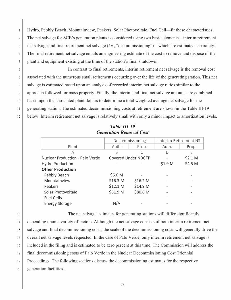
57

Hydro, Pebbly Beach, Mountainview, Peakers, Solar Photovoltaic, Fuel Cell—fit these characteristics. 1

The net salvage for SCE’s generation plants is considered using two basic elements—interim retirement 2

net salvage and final retirement net salvage (i.e., “decommissioning”)—which are estimated separately. 3

The final retirement net salvage entails an engineering estimate of the cost to remove and dispose of the 4

plant and equipment existing at the time of the station’s final shutdown. 5

In contrast to final retirements, interim retirement net salvage is the removal cost 6

associated with the numerous small retirements occurring over the life of the generating station. This net 7

salvage is estimated based upon an analysis of recorded interim net salvage ratios similar to the 8

approach followed for mass property. Finally, the interim and final net salvage amounts are combined 9

based upon the associated plant dollars to determine a total weighted average net salvage for the 10

generating station. The estimated decommissioning costs at retirement are shown in the Table III-19 11

below. Interim retirement net salvage is relatively small with only a minor impact to amortization levels. 12

Table III-19 Generation Removal Cost

The net salvage estimates for generating stations will differ significantly 13

depending upon a variety of factors. Although the net salvage consists of both interim retirement net 14

salvage and final decommissioning costs, the scale of the decommissioning costs will generally drive the 15

overall net salvage levels requested. In the case of Palo Verde, only interim retirement net salvage is 16

included in the filing and is estimated to be zero percent at this time. The Commission will address the 17

final decommissioning costs of Palo Verde in the Nuclear Decommissioning Cost Triennial 18

Proceedings. The following sections discuss the decommissioning estimates for the respective 19

generation facilities. 20

Plant Auth. Prop. Auth. Prop.A B C D E

Nuclear Production Palo Verde $2.1 MHydro Production $1.9 M $4.5 MOther ProductionPebbly Beach $6.6 MMountainview $16.3 M $16.2 MPeakers $12.1 M $14.9 MSolar Photovoltaic $81.9 M $80.8 MFuel CellsEnergy Storage N/A

Decommissioning

Covered Under NDCTP

Interim Retirement NS

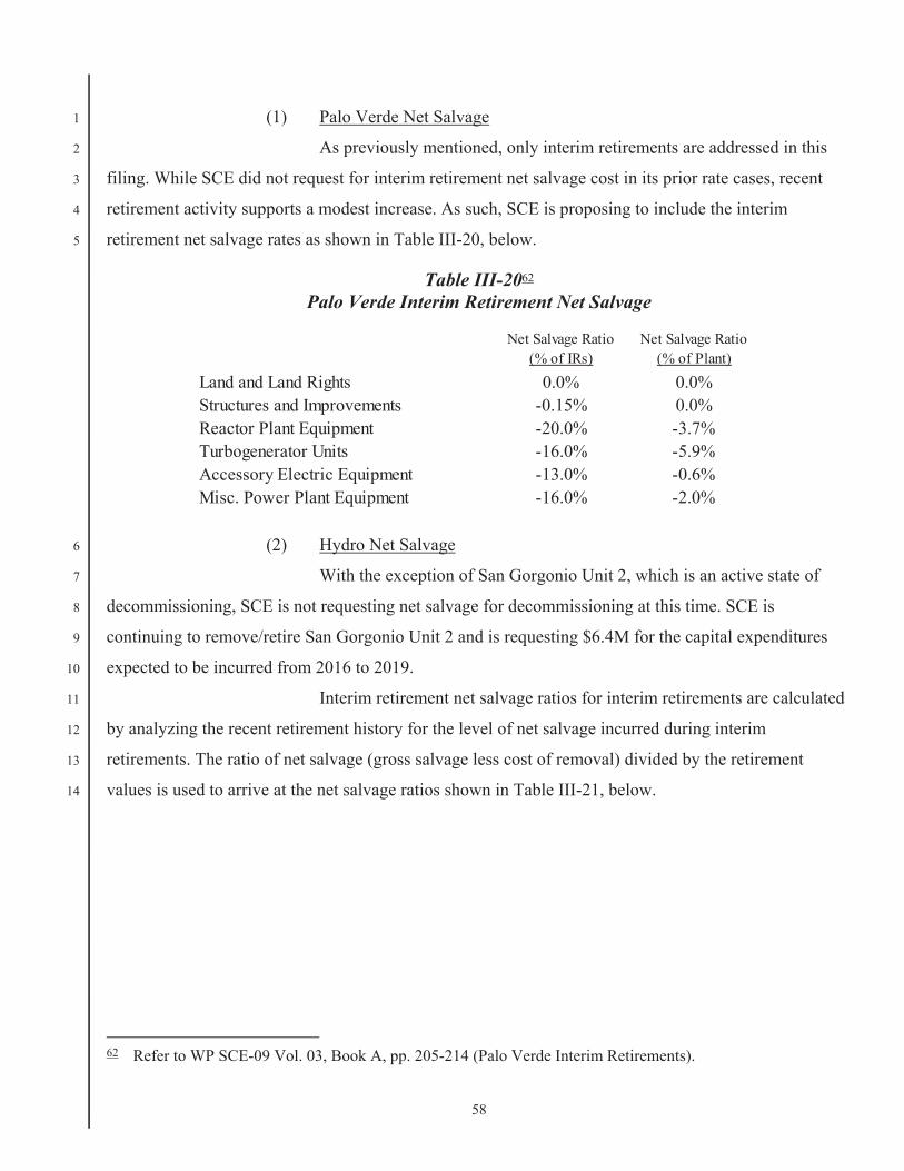
58

(1) Palo Verde Net Salvage 1

As previously mentioned, only interim retirements are addressed in this 2

filing. While SCE did not request for interim retirement net salvage cost in its prior rate cases, recent 3

retirement activity supports a modest increase. As such, SCE is proposing to include the interim 4

retirement net salvage rates as shown in Table III-20, below. 5

Table III-2062 Palo Verde Interim Retirement Net Salvage

(2) Hydro Net Salvage 6

With the exception of San Gorgonio Unit 2, which is an active state of 7

decommissioning, SCE is not requesting net salvage for decommissioning at this time. SCE is 8

continuing to remove/retire San Gorgonio Unit 2 and is requesting $6.4M for the capital expenditures 9

expected to be incurred from 2016 to 2019. 10

Interim retirement net salvage ratios for interim retirements are calculated 11

by analyzing the recent retirement history for the level of net salvage incurred during interim 12

retirements. The ratio of net salvage (gross salvage less cost of removal) divided by the retirement 13

values is used to arrive at the net salvage ratios shown in Table III-21, below. 14

62 Refer to WP SCE-09 Vol. 03, Book A, pp. 205-214 (Palo Verde Interim Retirements).

Net Salvage Ratio(% of IRs)

Net Salvage Ratio(% of Plant)

Land and Land Rights 0.0% 0.0%Structures and Improvements -0.15% 0.0%Reactor Plant Equipment -20.0% -3.7%Turbogenerator Units -16.0% -5.9%Accessory Electric Equipment -13.0% -0.6%Misc. Power Plant Equipment -16.0% -2.0%

59

Table III-2163 Hydro Interim Retirement Net Salvage

(3) Pebbly Beach Net Salvage 1

Due to the expectations that the diesel generators will continue to operate 2

in the foreseeable future, SCE is not proposing to recover any decommissioning costs in this rate case. 3

Because of limited retirement history, SCE is not proposing recovery of interim retirement net salvage at 4

this time. 5

(4) Mountainview Net Salvage 6

SCE compiled a list of equipment and facilities to be installed as part of 7

the new generation facilities and itemized them by FERC plant account.64 SCE then developed 8

demolition costs for each component. The estimated decommissioning costs for Mountainview is $8.9 9

million (2012 dollars). SCE escalated the $8.9 million out to the end of the remaining life of the station, 10

resulting in $16.265 million. Because of limited retirement history, SCE is not proposing recovery of 11

interim retirement net salvage at this time. 12

(5) Peakers Net Salvage 13

In 2007, SCE commissioned Arcadis to perform decommissioning cost 14

studies for each of its five Peaker units. Table III-22 below shows the current cost for each unit, totaling 15

$7.7M. Escalated to the estimated year of final retirement produces a total future decommissioning cost 16

of $14.9M.66 Because of limited retirement history, SCE is not proposing recovery of interim retirement 17

net salvage at this time. 18

63 Refer to WP SCE-09 Vol. 03, Book A, pp. 215-223 (Hydro Interim Retirements). 64 Refer to WP SCE-09 Vol. 03, Book A, pp. 308-313 (Mountainview Decomm). 65 Id. 66 Refer to WP SCE-09 Vol. 03, Book A, pp. 225-291 (Peakers Decomm).

Net Salvage Ratio(% of IRs)

Net Salvage Ratio(% of Plant)

Structures and Improvements -150% -10.9%Reservoirs, Dams and Waterways -250% -5.6%Water Wheels, Turbines & Generators -50% -9.5%Accessory Electric Equipment -150% -10.6%Misc. Power Plant Equipment -20% -1.9%Roads, Railroads & Bridges -100% -11.5%

60

Table III-22 Peaker Decommissioning Costs ($000’s)

(6) Solar Photovoltaic Net Salvage 1

In 2011, SCE commissioned Worley Parsons to conduct a 2

decommissioning study of its Solar Photovoltaic Equipment. The study resulted in a range of estimates 3

between $300,000 and $547,000 per megawatt in 2011 dollars based on the type of facility installed. 4

Lower cost estimates are associated with ground mount installations characterized by ease of access and 5

fewer equipment requirements, while the higher cost facilities are rooftop mounted that increase the 6

complexity of removal activities. Escalating the estimates to the end of the proposed 20-year average 7

service life results in a total decommissioning estimate of $81 million as shown in Table III-23. Because 8

of limited retirement history, SCE is not proposing recovery of interim retirement net salvage at this 9

time. 10

Table III-23 Solar Decommissioning Costs by Panel Type ($000’s)

(7) Fuel Cell Net Salvage 11

SCE is not proposing to recover decommissioning costs for Fuel Cells at 12

this time because of the expectation to transfer ownership to site hosts at the end of their 10-year life. 13

Line Peaker 2015 ($) Retirement Retirement YearNo. Unit Decomm Year Decomm ($)1. Barre $1,427 2042 $2,6762. Center $1,414 2042 $2,6523. Grapeland $1,593 2042 $2,9874. McGrath $1,683 2042 $3,1555. MiraLoma $1,604 2047 $3,407

$7,722 $14,877

Installation 2015 $ Installed Total Decomm Total DecommType Megawatt MW 2015 ($) Retirement Year ($)A B C D=B*C E

Rooftop Floating $614 54 $32,890 $47,959Rooftop Anchored $645 31 $20,071 $29,486Ground Mount $354 7 $2,395 $3,410

$55,355 $80,855

61

While SCE is not proposing decommissioning at this time, it is not unreasonable to expect that if 1

circumstances change, there will be future costs to retire these plants. 2

(8) Energy Storage Net Salvage 3

SCE is proposing to install lithium-ion battery units in a rack 4

configuration. Engineers indicate that the removal activities to retire these assets include driving to the 5

facility, removing the battery modules the rack, and shipping to recycling centers for disposal. Engineers 6

also indicate that there may be a small amount of gross salvage associated with the recycling of the 7

units. Although it is not unreasonable to assume that there may be increasing costs to retire these assets 8

in the future (e.g., if recycling salvage becomes disposal fees) SCE is not proposing decommissioning 9

costs for energy storage assets at this time. 10

3. Forecast Service Lives for G&I Assets 11

Some categories of plant do not lend themselves to statistical analysis, but do not belong 12

in the life span category. These plant assets include most general plant (i.e., FERC Accounts 391-397), 13

intangible plant (e.g., software, radio frequencies, etc.), and easements. SCE determined average service 14

lives through conducting discussions with SCE engineers familiar with the assets, considering prior 15

company procedure, and being familiar with industry practice. 16

Table III-24, below, shows the forecast depreciation service lives for general and 17

intangible plant accounts. The table compares SCE’s proposed depreciation rates to authorized service 18

lives from D.15-11-021 (the 2015 GRC Decision). As discussed in the sections below, because Power 19

Management Systems (Account 391.4) and Telecommunications Equipment (Account 397) consist of 20

sub-accounts of fairly disparate service lives, the subaccounts have been categorized based upon the 21

equipment lives. For example, in the case of Telecommunication Equipment, SCE grouped Telephone 22

Systems with Videoconferencing Equipment in a 7-year category separate from the infrastructure 23

equipment such as open wire communication conductor and antenna support structures that belong in a 24

40-year category. 25

62

Table III-2467 General and Intangible Plant Service Life Proposals

67 Refer to WP SCE-09 Vol. 03, Book A, pp. 5-12 (Rate Determination Schedule).

2015-2017 2018-2020Account Authorized Proposed

No. Account Description (Years) (Years)

General Plant391.1 Office Furniture 20 20391.2 Personal Computers 5 5391.3 Mainframe Computers 5 5391.4 DDSMS-Power Management System 7.8 10.2391.5 Office Equipment 5 5391.6 Duplicating Equipment 5 5391.7 PC Software 5 5393 Stores Equipment 20 20394 Tools & Work Equipment 10 10395 Laboratory Equipment 15 15397 Telecommunication Equipment 10.3 8.6398 Misc Power Plant Equipment 20 20

Intangibles302.020 Hydro Relicensing Various Various303.640 Radio Frequency 40 40302.050 Miscellaneous Intangibles 20 20303.105 Capitalized Software - 5 year 5 5303.707 Capitalized Software - 7 year 7 7303.210 Capitalized Software - 10 year 10 10303.315 Capitalized Software - 15 year 15 15

Easements350 Transmission Easements 60 60360 Distribution Easements 60 60389 General Easements 60 60

63

4. Forecast Service Lives – Account-By-Account 1

a) General Plant 2

Most general and intangible plant accounts contain many low value individual 3

items. Following FERC guidelines, non-structural items in these accounts are amortized by vintage 4

group over the specified service life and retired at the end of the life span.68 For example, personal 5

computers are amortized over a 5-year period (i.e., a 20 percent annual depreciation rate) and when a 6

vintage group reaches five years of age, the vintage group of computers will be fully depreciated and 7

retired off the books. Following this approach eliminates costly plant record keeping and continuous 8

physical tracking of the equipment. Over time, imbalances in the accumulated depreciation can occur if 9

there are depreciation life or rate changes and if net salvage is recorded to the books but not reflected in 10

the depreciation rate. These accumulated depreciation surpluses (deficits) are amortized over this GRC 11

cycle (2018-2020). 12

(1) Account 391.1 – Office Furniture 13

Account 391.1 contains all costs incurred to acquire office furniture. It 14

includes such items as modular furniture, desks, cabinets, and files used for general utility service that 15

are not permanently attached to buildings. A 20-year average service life is reasonable for both modular 16

and free standing furniture. 17

(2) Account 391.2 And 391.3 – Computer Equipment 18

The assets in Account 391.2 can include Central Processing Units and 19

associated components (e.g., monitors, printers, etc.) when purchased as a bundled unit, or when any of 20

these items are purchased individually and meet the capitalization threshold. Account 391.3 is where 21

SCE records all investment related to mainframe computer and file server equipment. SCE information 22

technology personnel state that the average life for this equipment should be five years or less. Retention 23

of the five-year life is reasonable. 24

(3) Account 391.4 – Power Management System 25

Account 391.4 contains Supervisory Control and Data Acquisition 26

(SCADA) equipment for controlling and monitoring the SCE electrical system. Contained within this 27

68 FERC Accounting Release Number AR15 provided for the vintage year accounting method allowing

companies to amortize vintage groups of assets over their designated service life and subsequently retire them. The FERC accounting release states that “[a]doption- of vintage year accounting will relieve companies from maintaining extensive plant records and will generate efficiencies and costs savings without degrading the quality of plant records and the associated financial reporting.”

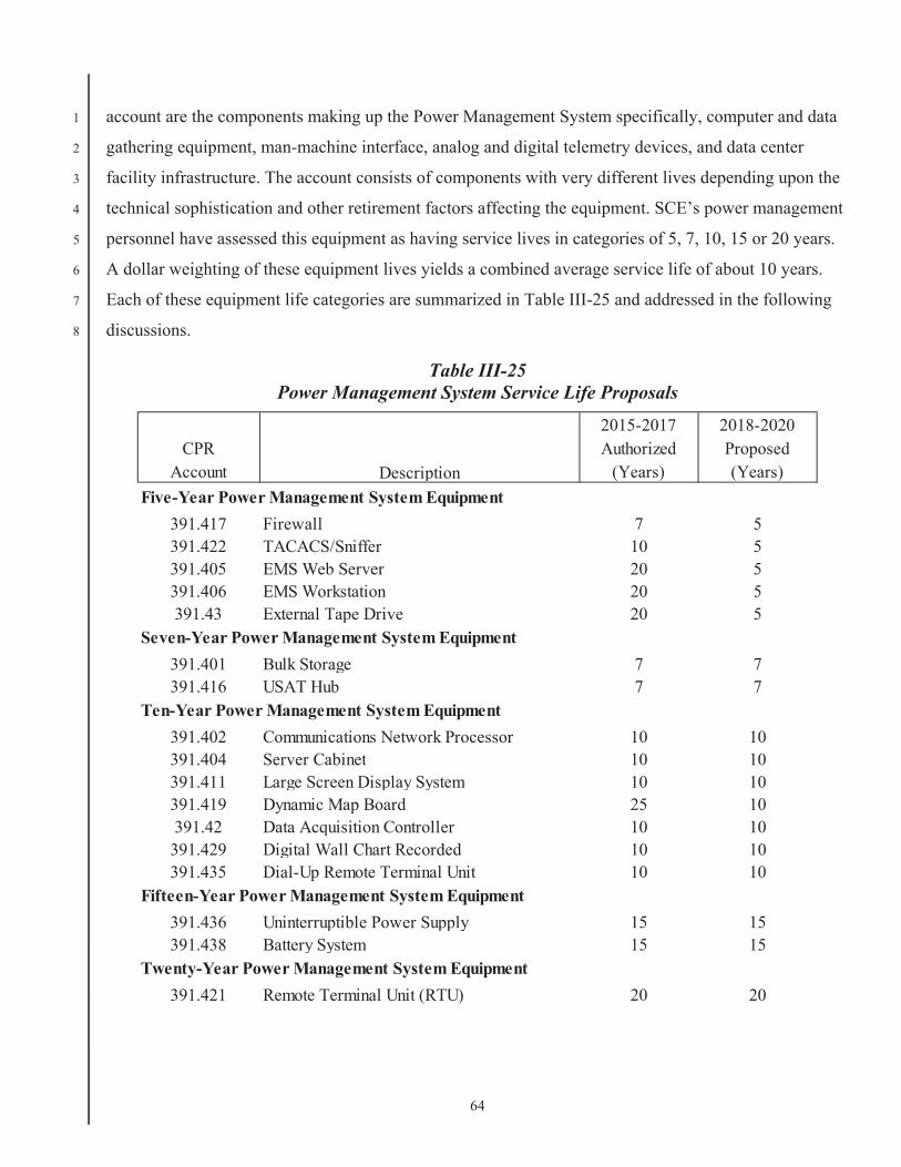
64

account are the components making up the Power Management System specifically, computer and data 1

gathering equipment, man-machine interface, analog and digital telemetry devices, and data center 2

facility infrastructure. The account consists of components with very different lives depending upon the 3

technical sophistication and other retirement factors affecting the equipment. SCE’s power management 4

personnel have assessed this equipment as having service lives in categories of 5, 7, 10, 15 or 20 years. 5

A dollar weighting of these equipment lives yields a combined average service life of about 10 years. 6

Each of these equipment life categories are summarized in Table III-25 and addressed in the following 7

discussions. 8

Table III-25 Power Management System Service Life Proposals

2015-2017 2018-2020CPR Authorized Proposed

Account (Years) (Years)

391.417 Firewall 7 5391.422 TACACS/Sniffer 10 5391.405 EMS Web Server 20 5391.406 EMS Workstation 20 5391.43 External Tape Drive 20 5

391.401 Bulk Storage 7 7391.416 USAT Hub 7 7

391.402 Communications Network Processor 10 10391.404 Server Cabinet 10 10391.411 Large Screen Display System 10 10391.419 Dynamic Map Board 25 10391.42 Data Acquisition Controller 10 10

391.429 Digital Wall Chart Recorded 10 10391.435 Dial-Up Remote Terminal Unit 10 10

391.436 Uninterruptible Power Supply 15 15391.438 Battery System 15 15

391.421 Remote Terminal Unit (RTU) 20 20

Fifteen-Year Power Management System Equipment

Twenty-Year Power Management System Equipment

DescriptionFive-Year Power Management System Equipment

Seven-Year Power Management System Equipment

Ten-Year Power Management System Equipment

65

(a) Five-Year Power Management System Equipment 1

Equipment in the 5-year category is typically modern, digital 2

electronic computer and microprocessor-based equipment which is subject to discontinued support by 3

the manufacturer or replaced with newer equipment within a short period of time. Due to these changing 4

needs, the hardware asset portfolio will become obsolete if not actively refreshed, which can 5

significantly affect operations. Furthermore, these devices contain components like processors, memory, 6

and rotating disks that become obsolete and/or worn out after five years of continuous use. 7

(b) Seven-Year Power Management System Equipment 8

Equipment in the 7-year category is typically modern, digital 9

electronic computer and microprocessor-based equipment which is subject to discontinued support by 10

the manufacturer or replaced with newer equipment within a short period of time. Furthermore, these 11

devices contain rotating disk, printers and CRTs that become obsolete and/or worn out after seven years 12

of continuous use. 13

(c) Ten-Year Power Management System Equipment 14

SCE’s power management personnel indicate that the ten-year 15

lived equipment is less sophisticated than the typical 7-year items. They contain digital electronics as 16

well as some electromechanical devices. Most of this equipment is specialized, proprietary and generally 17

supported by the vendor for 10 years. Past experience indicates this equipment will be replaced after 18

about 10 years. 19

(d) Fifteen-Year Power Management System Equipment 20

Telemetry equipment is analog devices with mostly repairable 21

parts. They do not contain a high degree of sophistication and with proper maintenance, these devices 22

should last approximately 15 years. The Uninterruptible Power System is an electromechanical device 23

with a rated life of about 15 years. Beyond 15 years both of these devices require high levels of 24

maintenance due to passive component failures and electromechanical malfunction. 25

(e) Twenty-Year Power Management System Equipment 26

Twenty-year power management system equipment contains 27

hardened substation field equipment used for data gathering. The equipment is highly fault-tolerant and 28

is typically supported by the vendor for approximately 20 years. Also included here are Wall Strip Chart 29

Recorders and Backup Control Systems. These are robust analog devices containing some passive 30

electronics typically rated for 20 years of service. 31

66

(4) Account 391.5 and 391.6 – Office Equipment; Duplicating Equipment 1

These accounts represent a $7.4 million net investment in miscellaneous 2

office equipment such as video projection equipment, public address equipment, plotters, duplicating 3

equipment, and so forth. The current service life of five years is reasonable. 4

(5) Account 393 – Stores Equipment 5

Account 393 represents a $7.6 million net investment in equipment used 6

for the receiving, shipping, handling, and storage of materials and supplies for warehouses. It includes 7

electric pallet jacks, lifting tables, stretch wrapping machine, racking rotobins/storage bins, battery 8

chargers, transformer trays, hand-held scanners, lockers, picking carts, awnings, barrel grabbers, 9

warehouse heaters, screen netting, cable cutting machines, and so forth. Based on historical Stores 10

Equipment usage and knowledge of warehouse equipment, the operational personnel state that this 11

equipment has a useful service life of 20 years or less. Retaining the current 20-year service life is 12

reasonable for this account. 13

(6) Account 394 – Tools & Work Equipment 14

Account 394 represents a $49.2 million net investment in tools and 15

equipment for construction, repair, maintenance, general shop, and garage, but not specifically 16

includable in other accounts. SCE proposes retaining the current service life of 10 years. 17

(7) Account 395 – Laboratory Equipment 18

Account 395 represents a $63.8 million net investment in laboratory and 19

field test equipment. The account has a wide variety of equipment. It includes, for example, calibrators, 20

baths, furnaces, current shunts, dew point meters, gauge calibrators, insulation testers, gas leak detectors, 21

mass comparator, micrometers, multimeters, oscilloscopes, phase meters, watthour meter testing power 22

source, power system analyzers, self-contained portable calibration carts, sound meters, metrology 23

standards, thermometer, vibration analysis data pack, and volt meters. The expected average service life 24

of lab and test equipment is impacted by two major retirement factors: technological obsolescence and 25

normal “wear and tear” from usage in both the field and lab environments. SCE proposes to retain the 26

currently authorized 15-year average service life for this account. 27

(8) Account 397 – Telecommunication Equipment 28

Account 397 represents SCE’s investment in communication equipment 29

for the company’s system. Contained within this account are the electronic and computer-based 30

equipment (such as transmission equipment, dynamic network multiplexers, data network 31

67

interconnection system, and radio equipment), as well as communication infrastructure (such as the 1

copper and fiber optic cable, conduit, microwave equipment, and the electrical power generator system). 2

SCE telecommunication engineers have assessed this equipment as having service lives of 5, 7, 10, 15, 3

25, or 40 years depending on the type of equipment. 69 These are the same service lives the Commission 4

authorized in the prior rate case. The equipment lives are addressed in the following discussions. 5

(a) Five-Year Communication Equipment 6

Equipment falling into the 5-year category experiences shorter 7

lives from lack of vendor support, facility relocations, and insufficient capacity to meet current demand. 8

(b) Seven-Year Communication Equipment 9

Equipment in the 7-year category is typically modern, state-of-the 10

art, electronic and/or computer-based equipment which is subject to being discontinued by manufacturer 11

or replaced with newer equipment within a short period of years. 12

(c) Ten-Year Communication Equipment 13

NetComm radio equipment is not as sophisticated as the other 14

electronic equipment and warrants a 10-year service life. SCE is replacing NetComm radios after about 15

10 years. 16

(d) Fifteen-Year Communication Equipment 17

Equipment in this group of assets is typically subject to 18

environmental wear and has an average life of about 15 years. The equipment fails or is replaced as a 19

result of unreliability and/or high maintenance due to failure of passive components or 20

electromechanical failure. In the case of electronic components included in this category, the 21

telecommunication engineers state that these are relatively basic and not the state-of-the art- electronics 22

reflected in the seven-year life category. 23

(e) Twenty-Five Year Communication Equipment 24

Although SCE has not yet had fiber optic cable as long as 25 years, 25

SCE telecommunication engineers believe that it may be subject to greater level of degradation than the 26

copper cable. They estimate that 25 years is a reasonable life for the fiber optic cable. 27

69 Refer to WP SCE-09 Vol. 03, Book A, pp. 314-318 (Telecomm. Engineering Data).

68

(f) Forty-Year Communication Equipment 1

The balance of the communication infrastructure includes such 2

equipment as overhead and underground communication cable, the communication conduit system, and 3

antenna support structures. This equipment has an average 40-year service life. The items are subject to 4

physical or mechanical deterioration since they are subject to outdoor environments. 5

(9) Account 398 – Miscellaneous 6

Account 398 represents a $21.8 million net investment in miscellaneous 7

utility equipment that does not fit other plant accounts. Examples can include such diverse items as 8

kitchen and infirmary equipment. The current service life of 20 years is a reasonable depreciation period 9

for this account. 10

b) Intangibles 11

SCE has investments in a number of intangible assets, including hydro 12

relicensing, radio frequencies, long term franchise fees, capitalized software, and land easements and 13

rights-of-way. As previously discussed, the hydro relicensing costs are amortized over the remaining life 14

of the FERC project license period. SCE proposes to continue amortizing the radio frequency 15

investments over the 40-year service life and land easements and rights-of-way over the 60 year service 16

life determined in prior rate case proceedings. The other categories are discussed below. 17

(1) Miscellaneous Intangibles 18

The year-end 2015 net investment for miscellaneous intangibles is 19

approximately $431 thousand, which is largely made up of long-term franchise costs (~$300 thousand). 20

SCE proposes to allocate these costs over 20 years. 21

(2) Capitalized Software 22

The depreciable life of capitalized software reflects the estimated life prior 23

to investments required to replace or optimize the software as a result of technology, vendor, or business 24

obsolescence. SCE proposes to continue the four existing service life categories of five, seven, ten, and 25

fifteen years determined in prior proceedings. 26

(3) Easements 27

SCE proposes to retain the authorized amortization period of 60 years for 28

its easements and rights-of-way. 29

Appendix A

2016 Service-Life and Net Salvage Study

2016 Service–life and Net Salvage Study

�

�

�

�

�

�

�

�

�

A1

CONTENTS

EXECUTIVE SUMMARY SECTION I INTRODUCTION .................................................................................................................. 1

SCOPE OF STUDY .............................................................................................................. 1

STUDY PROCEDURE SECTION II INTRODUCTION .................................................................................................................. 2

SCOPE .............................................................................................................................. 2

DATA COLLECTION ............................................................................................................ 3

LIFE ANALYSIS AND ESTIMATION ........................................................................................ 4

NET SALVAGE ANALYSIS .................................................................................................... 6

RECOMMENDATIONS AND ANALYSIS SECTION III RECOMMENDATIONS .......................................................................................................... 9

ANALYSIS .......................................................................................................................... 9 TRANSMISSION PLANT ACCOUNT 352.00 – STRUCTURES AND IMPROVEMENTS ................................................ 10 ACCOUNT 353.00 – STATION EQUIPMENT ..................................................................... 12 ACCOUNT 354.00 – TOWERS AND FIXTURES................................................................. 15 ACCOUNT 355.00 – POLES AND FIXTURES .................................................................... 17 ACCOUNT 356.00 – OVERHEAD CONDUCTORS AND DEVICES ........................................ 19 ACCOUNT 357.00 – UNDERGROUND CONDUIT .............................................................. 21 ACCOUNT 358.00 – UNDERGROUND CONDUCTORS AND DEVICES ................................. 23 ACCOUNT 359.00 – ROADS AND TRAILS ....................................................................... 25 DISTRIBUTION PLANT ACCOUNT 361.00 – STRUCTURES AND IMPROVEMENTS ................................................ 26 ACCOUNT 362.00 – STATION EQUIPMENT ..................................................................... 28 ACCOUNT 364.00 – POLES AND FIXTURES .................................................................... 30 ACCOUNT 365.00 – OVERHEAD CONDUCTORS AND DEVICES ........................................ 32 ACCOUNT 366.00 – UNDERGROUND CONDUIT .............................................................. 35 ACCOUNT 367.00 – UNDERGROUND CONDUCTORS AND DEVICES ................................. 37 ACCOUNT 368.00 – LINE TRANSFORMERS .................................................................... 39 ACCOUNT 369.00 – SERVICES ..................................................................................... 41 ACCOUNT 370.00 – METERS ....................................................................................... 43 ACCOUNT 373.00 – STREET LIGHTING AND SIGNAL SYSTEMS ....................................... 45 GENERAL PLANT ACCOUNT 390.00 – STRUCTURES AND IMPROVEMENTS ................................................ 47

� �August 2016

PAGE II PAGE II

A2

EXECUTIVE SUMMARY

INTRODUCTION This report presents a study and recommended service–life statistics and future net salvage rates for transmission, distribution and general depreciable plant owned and operated by Southern California Edison Company (SCE). Foster As-sociates was engaged by SCE in January 2016. The study was completed in July, 2016.

Foster Associates is a public utility economics consulting firm offering economic research and consulting services on issues and problems arising from governmen-tal regulation of business. Areas of specialization supported by the firm’s Fort Myers office include property life forecasting, technological forecasting, depre-ciation estimation, and valuation of industrial property.

Foster Associates has undertaken numerous depreciation engagements for both public and privately owned business entities including detailed statistical life stud-ies, analyses of required net salvage rates, and the selection of depreciation sys-tems that will most nearly achieve the goals of depreciation accounting under the constraints of either government regulation or competitive market pricing. Foster Associates is widely recognized for industry leadership in the development of de-preciation systems, life analysis techniques and computer software for conducting depreciation and valuation studies.

Depreciation rates currently used by SCE were approved by the California Public Utilities Commission (CPUC) in D.15–11–021, dated November 5, 2015. The ap-proved rates were derived from a study conducted on December 31, 2012 plant and depreciation reserve balances. Findings and recommendations developed in the current study are summarized in Section III of this report. SCOPE OF STUDY The principal activities undertaken in the course of the current study included:

� Collection of plant and net salvage data; � Reconciliation of data to the official records of the Company; � Field visits and discussions with SCE operations and plant accounting

personnel; � Statistical life studies and estimation of projection lives and projec-

tion curves; and � Per unit and moving average net salvage studies and estimation of

future net salvage rates. �

� �

PAGE 1

A3

STUDY PROCEDURE

INTRODUCTION The purpose of a comprehensive depreciation study for a regulated utility is to an-alyze the mortality characteristics, net salvage rates and the adequacy of deprecia-tion accruals derived from currently approved depreciation rates. The findings from such an investigation are used in the formulation of revised depreciation rates subject to regulatory approvals.

In the case of the current study, Foster Associates was engaged by SCE to only study and recommend service–life statistics and future net salvage rates in com-pliance with CPUC directives in D.15–11–021. SCE would then incorporate the recommendations in depreciation rates developed by the Company.

Regarding the directives in D.15–11–021, the CPUC directed SCE to provide full explanations of the quantitative or qualitative base for the application of judgment in future depreciation showings. The Commission further directed the Company to provide:

1. A quantitative discussion of historical and future COR on a per unit ba-sis for the large (greater than 15% as measured by the portion of plant balance) asset classes in the account. This should identify and explain the key factors in changing or maintaining the per–unit COR.

2. Quantitative discussion of historical and future retirement mix; identi-fying and explaining the key factors in changing or maintaining this mix.

3. Quantitative discussion of asset life and original cost of assets being re-tired, in relation to the COR, on both a historical and prospective basis. This discussion should be integrated with and/or cross–reference the proposal for life characteristics.

4. An account–specific discussion of the process for allocating costs to COR.

SCOPE The steps involved in conducting the depreciation study can be grouped into three major tasks:

� Data Collection; � Life Analysis and Estimation; and � Net Salvage Analysis and Estimation.

The scope of the 2016 service–life and net salvage study included a consideration of each of these tasks as described below.

PAGE 2

A4

DATA COLLECTION The minimum database required to conduct a statistical life study consists of a history of vintage year additions and unaged activity–year retirements, transfers and adjustments. These data must be appropriately adjusted for transfers, sales and other plant activity that would otherwise bias the measured service life of normal retirements. The age distribution of surviving plant for unaged data can be estimated by distributing plant in service at the beginning of the study year to pri-or vintages in proportion to the theoretical amount surviving from a projection or survivor curve identified in the life study. The statistical methods of life analysis used to examine unaged plant data are known as semi–actuarial techniques.

A far more extensive database is required to apply statistical methods of life anal-ysis known as actuarial techniques. Plant data used in an actuarial life study most often include age distributions of surviving plant at the beginning of a study year and the vintage year, activity year, and dollar amounts associated with normal re-tirements, reimbursed retirements, sales, abnormal retirements, transfers, correc-tions, and extraordinary adjustments over a series of prior activity years. An actu-arial database may include age distributions of surviving plant at the beginning of the earliest activity year, rather than at the beginning of the study year. Plant addi-tions, however, must be included in a database containing an opening age distri-bution to derive aged survivors at the beginning of the study year. All activity year transactions with vintage year identification are coded and stored in a data-base. These data are processed by a computer program and transaction summary reports are created in a format reconcilable to official plant records. The availabil-ity of such detailed information is dependent upon an accounting system that sup-ports aged property records. The Continuing Property Record (CPR) system used by SCE provides aged transactions for all plant accounts.

Service life statistics estimated in the 2016 study were derived from plant ac-counting transactions recorded over the period 2002 through 2015. Detailed ac-counting transactions were extracted from the Continuing Property Record (CPR) system and assigned transaction codes which describe the nature of the account-ing activity. Transaction codes for plant additions, for example, were used to dis-tinguish normal additions from acquisitions, purchases, reimbursements and ad-justments. Similar transaction codes were used to distinguish normal retirements from sales, reimbursements, abnormal retirements and adjustments. Transaction codes were also assigned to transfers, capital leases, gross salvage, cost of remov-al and other accounting activity that should be considered in a depreciation study.

The accuracy and completeness of the assembled database was verified for activi-ty years 2002 through 2015 by comparing the beginning plant balance, additions, retirements, transfers and adjustments, and the ending plant balance derived for each activity year to the official plant records of the Company. Age distributions of surviving plant at December 31, 2015 were reconciled to the CPR.

PAGE 3

�

A5

LIFE ANALYSIS AND ESTIMATION Life analysis and life estimation are terms used to describe a two–step procedure for estimating the mortality characteristics of a plant category. The first step (i.e., life analysis) is largely mechanical and primarily concerned with history. Statisti-cal techniques are used in this step to obtain a mathematical description of the forces of retirement acting upon a plant category and an estimate of the projection life of the account. The mathematical expressions used to describe these life char-acteristics are known as survival functions or survivor curves.

It is important to note what is being estimated in a service life study. It is not unit-years of service; it is dollar–years of service. Retirements are not recorded for plant accounting purposes in units such as feet, pounds, segments or any similar physical measurement. Plant records are maintained in dollars and service lives are measured in dollar–years of service. Estimating service lives based on engi-neering studies of how long, on average, units of property might remain in service is not equivalent to estimating dollar–years of service.

The size of a retirement unit also matters. A company that defines a span of con-ductor between supports to be a retirement unit will measure longer service lives than a company that defines one foot of conductor as a retirement unit. Replace-ment of conductor less than a retirement unit is charged to operating expense and no retirement is recorded for the replaced unit. Larger units result in less frequent recorded retirements, which translate to longer average dollar–years of service.

An added dimension of complexity is introduced when retirements occur at vary-ing ages, attributable to mixed forces of retirement. This creates a non-homogeneous account composed of two subpopulations acted upon by differing forces of retirement. The estimated projection life for such an account measured in dollar–years of service will converge toward the mean of the subpopulation most resistant to the forces of retirement.

The second step (i.e., life estimation) is concerned with predicting the expected remaining life of property units still exposed to forces of retirement. It is a process of blending the results of a life analysis with informed judgment (including expec-tations about the future) to obtain an appropriate projection life and curve descrip-tive of the parent population from which a plant account is viewed as a random sample. The amount of weight given to a life analysis will depend upon the extent to which past retirement experience is considered descriptive of the future.

The analytical methods used in a life analysis are broadly classified as actuarial and semi–actuarial techniques. Actuarial techniques can be applied to plant ac-counting records that reveal the age of a plant asset at the time of its retirement from service. Stated differently, each property unit must be identifiable by date of installation and age at retirement. Semi–actuarial techniques can be used to derive service life and dispersion estimates when age identification of retirements is not

PAGE 4

�

A6

maintained or readily available. Age identification of retirements over the period 2002–2015 was available for all plant accounts included in the 2016 study.

An actuarial life analysis program designed and developed by Foster Associates was used in this study. The first step in an actuarial analysis involves a systematic treatment of the available data for the purpose of constructing an observed life ta-ble. A complete life table contains the life history of a group of property units in-stalled during the same accounting period and various probability relationships derived from the data. A life table is arranged by age–intervals (usually defined as one year) and shows the number of units (or dollars) entering and leaving each age–interval and probability relationships associated with this activity. A life table minimally shows the age of each survivor and the age of each retirement from a group of units installed in a given accounting year.

A life table can be constructed in any one of at least five methods. The annual–rate or retirement–rate method was used in this study. The mechanics of the annu-al–rate method require the calculation of a series of ratios obtained by dividing the number of units (or dollars) surviving at the beginning of an age interval into the number of units (or dollars) retired during the same interval. This so–called “retirement ratio” (or set of ratios) is an estimator of the hazard rate or conditional probability of retirement during an age interval. The cumulative proportion sur-viving is obtained by multiplying the retirement ratio for each age interval by the proportion of the original group surviving at the beginning of that age interval and subtracting this product from the proportion surviving at the beginning of the same interval. The annual–rate method is applied to multiple groups or vintages by combining the retirements and/or survivors of like ages for each vintage in-cluded in the analysis.

The second step in an actuarial analysis involves graduating or smoothing the ob-served life table and fitting the smoothed series to a family of survival functions. The functions used in this study are the Iowa–type curves which are mathemati-cally described by the Pearson frequency curve family. Observed life tables were smoothed by a weighted least–squares procedure in which first, second and third degree orthogonal polynomials were fitted to the observed retirement ratios. The resulting function was expressed as a survivorship function and numerically inte-grated to obtain an estimate of the projection life for each plant account. The smoothed survivorship function was then fitted by a weighted least–squares pro-cedure to the Iowa–curve family to obtain a mathematical description or classifi-cation of the dispersion characteristics of the data.

The set of computer programs used in this analysis provides multiple rolling–band, shrinking–band and progressive–band analyses of an account. Observation bands are defined in terms of a "retirement era" that restricts the analysis to the re-tirement activity of all vintages represented by survivors at the beginning of a se-lected era. In a rolling–band analysis, a year of retirement experience is added to

�

PAGE 5

A7

each successive retirement band and the earliest year from the preceding band is dropped. A shrinking–band analysis begins with the total retirement experience available and the earliest year from the preceding band is dropped for each suc-cessive band. A progressive–band analysis adds a year of retirement activity to a previous band without dropping earlier years from the analysis. Rolling, shrinking and progressive band analyses are used to detect the emergence of trends in the behavior of the dispersion and projection life.

Options available in the Foster Associates actuarial life analysis program include: the width and location of both placement and observation bands; the interval of years included in a selected band analysis; the estimator of the hazard rate (actuar-ial, conditional proportion retired, or maximum likelihood); the elements to in-clude on the diagonal of a weight matrix (exposures, inverse of age, inverse of variance, or unweighted); and the age at which an observed life table is truncated. The program also provides tabular and graphics output as an aid in the analysis.

While actuarial and semi–actuarial statistical methods are well suited to an analy-sis of plant categories containing a large number of homogeneous units (e.g., poles and conductors), the concept of retirement dispersion is interpreted differ-ently for plant categories composed of major items of plant that will most likely be retired as a single unit. Plant retirements from an integrated system prior to the retirement of the entire facility are more properly viewed as interim retirements that will be replaced in order to maintain the integrity of the system. Additionally, plant facilities may be added to the existing system (i.e., interim additions) in or-der to expand or enhance its productive capacity without extending the service life of the existing system. A proper depreciation rate can be developed for an inte-grated system using a life–span method. All depreciable plant accounts classified in transmission, distribution and general were studied as full mortality categories in the 2016 study.

NET SALVAGE ANALYSIS Depreciation rates designed to achieve the goals and objectives of depreciation accounting will include a parameter for future net salvage and a variable for aver-age net salvage reflecting both realized and future net salvage rates.

Estimates of net salvage rates applicable to future retirements are most often de-rived from an analysis of gross salvage and cost of removal realized in the past. An analysis of past experience (including an examination of trends over time) provides a reasonable basis for estimating future salvage and cost of removal. However, consideration should also be given to events that may cause deviations from net salvage realized in the past. Among the factors that should be considered are: the age of plant retirements; the portion of retirements likely to be reused; changes in the method of removing plant; the type of plant to be retired in the fu-ture; inflation expectations; the shape of the projection life curve; and economic

��

PAGE 6

A8

conditions that may warrant greater or lesser weight to be given to net salvage rates observed in the past.

Average net salvage rates for an account or plant function are derived from a di-rect dollar weighting of a) historical retirements with historical (or realized) net salvage rates and b) future retirements (i.e., surviving plant) with the estimated fu-ture net salvage rate. Average net salvage rates will change, therefore, as addi-tional years of retirement and net salvage activity become available and as subse-quent plant additions alter the weighting of future net salvage estimates.

Special consideration should also be given to the treatment of insurance proceeds and other forms of third–party reimbursements credited to the depreciation re-serve. A properly conducted net salvage study will exclude such activity from the estimate of future parameters and include the activity in the computation of real-ized and average net salvage rates.

A five–year moving average analysis of the ratio of realized salvage and removal expense to the associated retirements was conducted in the 2016 study for trans-mission, distribution and general plant categories to aid in: a) estimating a real-ized net salvage rate; b) detecting the emergence of historical trends; and c) estab-lishing a basis for estimating a future net salvage rate. Cost of removal and sal-vage opinions obtained from Company personnel were also considered in the es-timation of future net salvage rates.

In compliance with the CPUC directive in D.15–11–021, per unit net salvage analyses were conducted for the nine (9) plant accounts listed in Table 1 below.

Each of the nine plant accounts was grouped into one or more subpopulations of major equipment categories. Historical per unit ratios (defined as net cost per unit to retire divided by the cost per unit to install) were used in both a historical and future per unit analyses. Net costs to retire (or net salvage) were used in the analy-sis to maintain consistency with future net salvage parameters used in the formu-lation of remaining–life accrual rates.

Future per unit ratios were derived using an average of the subpopulation net sal-

��

PAGE 7

��

Account Description

354.00 Towers and Fixtures355.00 Poles and Fixtures356.00 Overhead Conductors and Devices364.00 Poles, Towers and Fixtures365.00 Overhead Conductors and Devices366.00 Underground Conduit367.00 Underground Conductors and Devices368.00 Line Transformers369.00 Services

Table 1. Per Unit Net Salvage Accounts

A9

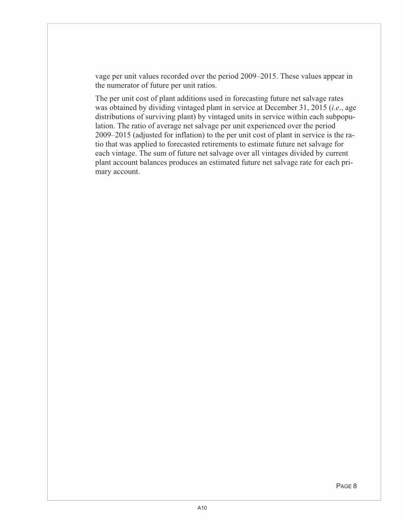
vage per unit values recorded over the period 2009–2015. These values appear in the numerator of future per unit ratios.

The per unit cost of plant additions used in forecasting future net salvage rates was obtained by dividing vintaged plant in service at December 31, 2015 (i.e., age distributions of surviving plant) by vintaged units in service within each subpopu-lation. The ratio of average net salvage per unit experienced over the period 2009–2015 (adjusted for inflation) to the per unit cost of plant in service is the ra-tio that was applied to forecasted retirements to estimate future net salvage for each vintage. The sum of future net salvage over all vintages divided by current plant account balances produces an estimated future net salvage rate for each pri-mary account.

�

PAGE 8

�

A10

RECOMMENDATIONS AND ANALYSIS

RECOMMENDATIONS Table 2 below provides a summary of current and recommended projection lives, projection curves and future net salvage rates estimated for SCE in the 2016 study.

ANALYSIS A description of each account examined in the 2016 study and factors considered in the estimation of recommended service life and net salvage parameters is con-tained in the following pages of this report.

�

PAGE 9

Current RecommendedAccount Description P-Life Dispersion Sf % P-Life Dispersion Sf %

A C D E F G H

Transmission Plant 352.00 Structures and Improvements 55.00 S3 -35.0 55.00 L1 -35.0353.00 Station Equipment 45.00 R0.5 -15.0 40.00 L0.5 -10.0354.00 Towers and Fixtures 65.00 R5 -60.0 65.00 R5 -185.0355.00 Poles and Fixtures 50.00 R0.5 -72.0 65.00 SC -499.0356.00 Overhead Conductors and Devices 61.00 R3 -80.0 61.00 R3 -210.0357.00 Underground Conduit 55.00 R3 0.0 55.00 R3 0.0358.00 Underground Conductors and Devices 40.00 R2.5 -15.0 45.00 S1 -25.0359.00 Roads and Trails 60.00 SQ 0.0 60.00 R5 0.0

Distribution Plant 361.00 Structures and Improvements 42.00 R2.5 -25.0 50.00 L0.5 -30.0362.00 Station Equipment 45.00 R1.5 -25.0 65.00 L0.5 -50.0364.00 Poles, Towers and Fixtures 47.00 L0.5 -210.0 55.00 R1 -488.0365.00 Overhead Conductors and Devices 45.00 R0.5 -115.0 55.00 R0.5 -538.0366.00 Underground Conduit 59.00 R3 -30.0 59.00 R3 -401.0367.00 Underground Conductors and Devices 45.00 R0.5 -60.0 43.00 R1.5 -261.0368.00 Line Transformers 33.00 R1 -20.0 33.00 S1.5 -47.0369.00 Services 45.00 R1.5 -100.0 45.00 R1.5 -387.0370.00 Meters 20.00 R3 -5.0 20.00 R3 0.0373.00 Street Lighting and Signal Systems 40.00 L0.5 -30.0 48.00 L1 -100.0

General Plant390.00 Structures and Improvements 38.00 R3 -5.0 45.00 R0.5 -10.0

Table 2. Service Life and Net Salvage Parameters

A11

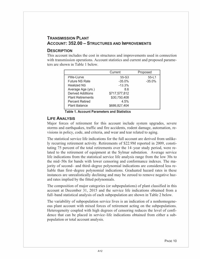
TRANSMISSION PLANT ACCOUNT: 352.00 – STRUCTURES AND IMPROVEMENTS DESCRIPTION This account includes the cost in structures and improvements used in connection with transmission operations. Account statistics and current and proposed parame-ters are shown in Table 1 below.

LIFE ANALYSIS Major forces of retirement for this account include system upgrades, severe storms and earthquakes, traffic and fire accidents, rodent damage, automation, re-visions in policy, code, and criteria, and wear and tear related to aging.

The statistical service life indications for the full account are derived from unlike-ly recurring retirement activity. Retirements of $22.9M reported in 2009, consti-tuting 75 percent of the total retirements over the 14–year study period, were re-lated to the retirement of equipment at the Sylmar substation. Average service life indications from the statistical service life analysis range from the low 30s to the mid–50s for bands with lower censoring and conformance indexes. The ma-jority of second– and third–degree polynomial indications are considered less re-liable than first–degree polynomial indications. Graduated hazard rates in these instances are unrealistically declining and may be zeroed to remove negative haz-ard rates implied by the fitted polynomials.

The composition of major categories (or subpopulations) of plant classified in this account at December 31, 2015 and the service life indications obtained from a full–band statistical analysis of each subpopulation are shown in Table 2 below.

The variability of subpopulation service lives is an indication of a nonhomogene-ous plant account with mixed forces of retirement acting on the subpopulations. Heterogeneity coupled with high degrees of censoring reduces the level of confi-dence that can be placed in service–life indications obtained from either a sub-population or total account analysis.

��

PAGE 10

Current ProposedPlife-Curve 55-S3 55-L1Future NS Rate -35.0% -35.0%Realized NS -13.3%Average Age (yrs.) 8.6Derived Additions $717,577,812Plant Retirements $30,750,408Percent Retired 4.5%Plant Balance $686,827,404

Table 1. Account Parameters and Statistics

A12

LIFE ESTIMATION Based mainly on the first–degree statistical service–life indications, thereby re-jecting origin–modal dispersions in which chance is a more pervasive force of re-tirement, a 55–L1 projection life–curve is recommended for this account. This recommendation retains the currently approved projection life and adjusts the pro-jection curve to reflect lower modal curves observed in the subpopulation analy-sis. The recommendation also reflects a lack of evidence for adjusting the service life estimates given the single retirement underlying a significant percentage of the retirement history. Foster Associates was informed that Company engineers and operations personnel do not anticipate policy or procedural changes or tech-nological advances that would introduce significantly different forces of retire-ment from those observed in the past.

NET SALVAGE ANALYSIS The adjusted historical net salvage analysis for this account exhibits an overall re-alized net salvage rate of –13.3 percent from $31M of retirement activity over the period 2002–2015. More recent 5–year moving average bands indicate realized negative net salvage exceeding –87 percent.

NET SALVAGE ESTIMATION Based on this historical experience and the expectation of continuing removal costs when these facilities are retired, retention of a –35 percent future net salvage rate is recommended for consideration by SCE. As in the service life estimation, this recommendation reflects lack of evidence for adjusting future net salvage es-timates given the single retirement underlying a significant percentage of the re-tirement history in this account.

�

��

PAGE 11

Investment Full Band CensoringCategory Amount ($) % PLife-Curve (%)

Foundations 178,220,072 26 85-L1 38.5 MEER Building 159,486,338 23 130-R0.5 73.4 Water Supply 107,675,420 16 103-R3 82.8 Alarm & Monitoring 45,931,434 7 194-S6 99.4 Power Lighting 30,490,714 4 107-L0.5 71.9 HVAC 12,046,998 2 38-L0 7.7 Non-unitized 120,611,640 18 Miscellaneous 32,364,788 5 30-L0.5 3.7

Total 686,827,404 100 107Table 2. Major Structural Components

A13

TRANSMISSION PLANT ACCOUNT: 353.00 – STATION EQUIPMENT DESCRIPTION This account includes the cost in transforming, conversion, and switching equip-ment used for the purpose of changing the characteristics of electricity in connec-tion with its transmission or for controlling transmission circuits. Account statis-tics and current and proposed parameters are shown in Table 1 below.

LIFE ANALYSIS Retirement activity in transmission station equipment is largely associated with age, obsolescence and growing or shifting loads that necessitate rebuilding to larger capacities. Company engineers report that thermal, mechanical, and electri-cal integrity issues intensify with age typically beginning around age 30 years when insulation degradation, increased in–service failures, and increased mainte-nance arises. Retirements occur when increased costs and decreased utilization rates dictate is it no longer economic to repair such equipment. Decreased spare parts availability as equipment ages also plays a major role in age–related retire-ments.

The Company utilizes a Condition Based Maintenance (CBM) approach to man-age all transformers and circuit breakers by routinely conducting off–line diagnos-tics, visual inspections, and functional checks. These analysis components are combined with other key data such as age, design, moisture levels, loading, and fault exposure to develop a health index ranking that is maintained throughout the life of these assets and used in the determination of when to repair or retire.

Average service life indications from the statistical analysis of the full account range from the low 30s to the low–40s for bands with lower censoring and con-formance indexes. The majority of second– and third–degree polynomial indica-tions are considered less reliable than first–degree polynomial indications. Gradu-ated hazard rates in these instances are unrealistically declining and may be ze-roed to remove negative hazard rates implied by the fitted polynomials.

�

PAGE 12

A14

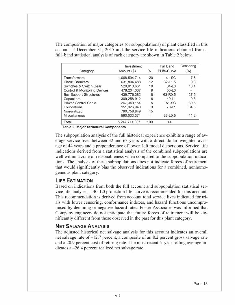
The composition of major categories (or subpopulations) of plant classified in this account at December 31, 2015 and the service life indications obtained from a full–band statistical analysis of each category are shown in Table 2 below.

The subpopulation analysis of the full historical experience exhibits a range of av-erage service lives between 32 and 63 years with a direct–dollar–weighted aver-age of 44 years and a preponderance of lower–left modal dispersions. Service–life indications derived from a statistical analysis of the combined subpopulations are well within a zone of reasonableness when compared to the subpopulation indica-tions. The analysis of these subpopulations does not indicate forces of retirement that would significantly bias the observed indications for a combined, nonhomo-geneous plant category.

LIFE ESTIMATION Based on indications from both the full account and subpopulation statistical ser-vice life analyses, a 40–L0 projection life–curve is recommended for this account. This recommendation is derived from account total service lives indicated for tri-als with lower censoring, conformance indexes, and hazard functions uncompro-mised by declining or negative hazard rates. Foster Associates was informed that Company engineers do not anticipate that future forces of retirement will be sig-nificantly different from those observed in the past for this plant category.

NET SALVAGE ANALYSIS The adjusted historical net salvage analysis for this account indicates an overall net salvage rate of –12.7 percent, a composite of an 8.2 percent gross salvage rate and a 20.9 percent cost of retiring rate. The most recent 5–year rolling average in-dicates a –26.4 percent realized net salvage rate.

�

�

PAGE 13

Full Band CensoringCategory Amount ($) % PLife-Curve (%)

Transformers 1,068,594,714 20 41-SC 7.6 Circuit Breakers 631,804,488 12 32-L1.5 0.8 Switches & Switch Gear 520,013,661 10 34-L0 10.4 Control & Monitoring Devices 478,204,337 9 50-L0 - Bus Support Structures 439,776,382 8 63-R0.5 27.5 Capacitors 309,258,912 6 49-L1 0.6 Power Control Cable 267,340,154 5 51-SC 30.6 Foundations 151,926,940 3 70-L1 34.5 Non-unitized 790,758,849 15 Miscellaneous 590,033,371 11 36-L0.5 11.2

Total 5,247,711,807 100 44Table 2. Major Structural Components

Investment

A15

NET SALVAGE ESTIMATION Minimal gross salvage, generally from scrap metal and recycling, is expected from the retirement of this equipment. Significant cost of retiring, however, is ex-pected in the form of labor and equipment such as cranes. The adjusted historical net salvage experience provides the basis for recommending a –10 percent future net salvage rate for consideration by SCE. This recommendation reflects dis-counting indications obtained from small retirements and large cost of removal recorded in 2015 and focusing more on activity years 2009�2014. The –12.7 real-ized net salvage rate and –26.4 percent realized net salvage rate observed for the most recent 5–year rolling band are somewhat distorted by the 2015 activity, which is not considered indicative of future expectations.

�

�

PAGE 14

A16

TRANSMISSION PLANT ACCOUNT: 354.00 – TOWERS AND FIXTURES DESCRIPTION This account includes the cost installed of towers and appurtenant fixtures used for supporting overhead transmission conductors. Account statistics and current and proposed parameters are shown in Table 1 below.

LIFE ANALYSIS Forces of retirement acting upon transmission towers and fixtures include line up-grades, corrosion, relocation (for lower voltage structures), and failures due to wind storms, ice, or floods. Most of these forces tend to increase with age. Alt-hough storm damage can generally be expected to impact retirements at any age, in combination with deterioration, the probability of failure is cumulative. SCE performs annual inspections on all transmission towers and performs subsequent maintenance identified from those inspections.

The statistical service life indications for the full account are derived from mini-mal and irregular retirement activity. Retirements recorded in this account amount to only $4.5M from an average plant balance exceeding $1.3B over the study pe-riod and less than 0.2 percent of derived additions. Statistical service life indica-tions derived from this minimal experience are highly censored, unrealistically long (approaching 200 years), and contrary to Company expectations of the future age of tower retirements.

The distribution of major categories of plant classified in this account at Decem-ber 31, 2015 and the service life indications obtained from a full–band statistical analysis of each category are shown in Table 2 below.

�

PAGE 15


Towers 1,139,621,027 50 132-S2 71.6 Non-unitized 1,018,898,065 45Other 101,453,734 4 178-R2.5 82.2


Investment

A17

The subpopulation analysis is also highly censored and does not produce interpre-tative life indications. The account could not be reasonably sub–divided into more than three subpopulations with miscellaneous items constituting only four percent and non–unitized items constituting 45 percent of the investment.

LIFE ESTIMATION The minimal retirement activity and resulting unreliable service life indications from both the full account and subpopulation statistical analyses do not provide a strong foundation for service–life estimation. Foster Associates, therefore, de-ferred to SCE in recommending the currently approved 65–R5 projection life–curve. Factors evaluated by SCE beyond the service–life analyses include opera-tional, accounting and ratemaking considerations.

NET SALVAGE ANALYSIS The adjusted net salvage analysis for this account indicates an overall net salvage rate of –799.7 percent realized from $4.5M of retirements recorded over the peri-od 2002–2015. However, as noted above, total retirements are less than 0.2% of derived additions.

The per–unit net salvage analysis conducted for this account indicates future net salvage rates ranging between –104 and –185 percent, depending upon the rate of future inflation. Inflation rates ranging between zero and 2.72 percent were as-sumed in the analysis. Future net salvage rates would increase with longer projec-tion lives and/or lower modal retirement dispersions.

NET SALVAGE ESTIMATION Although minimal gross salvage, generally from scrap, is expected from these as-sets, significant costs of retiring and removing (attributable to labor costs and cost of equipment such as cranes used in the retirement process) are expected to be in-curred in the future. Based on the above analysis, a future net salvage rate of �185 percent (derived from a 2.72 percent inflation rate) is recommended for considera-tion by SCE.

�

PAGE 16

A18

TRANSMISSION PLANT ACCOUNT: 355.00 – POLES AND FIXTURES DESCRIPTION This account includes the installed cost of transmission line poles, wood, steel, concrete, or other material, together with appurtenant fixtures used for supporting overhead transmission conductors. Account statistics and current and proposed parameters are shown in Table 1 below.

LIFE ANALYSIS The majority of wood poles in the Company's system are full–length and "through–boring" treated to protect against decay and insect attack. Wood poles may also be treated with a steel stub or a fiberglass wrap to provide additional support. In addition to pole treatment, the Company conducts a 10–year inspec-tion cycle to address safety and reliability. Tree trimming and vegetation man-agement are also a significant component of reliability measures undertaken by the Company.

Major forces of retirement acting upon transmission wood poles include external, internal, top rot, and split top deterioration. Additional forces include vehicles, wind, storm, fire, and bird (mainly woodpecker) damage. Response to these forc-es partly depends on the specific locale of the pole given the Company's wide ge-ographical area encompassing mainly desert but also agricultural, rural, and urban communities.

Indications from the statistical service life analysis for this account range from the mid–60s to the low–80s for bands with lower censoring and conformance indexes. The majority of third–degree polynomial indications are considered less reliable than first–degree or second–degree polynomial indications. Graduated hazard rates in these instances are unrealistically declining and may be zeroed to remove negative hazard rates implied by the fitted polynomials.

The composition of major categories (or subpopulations) of plant classified in this account at December 31, 2015 and the service life indications obtained from a

�

PAGE 17

A19

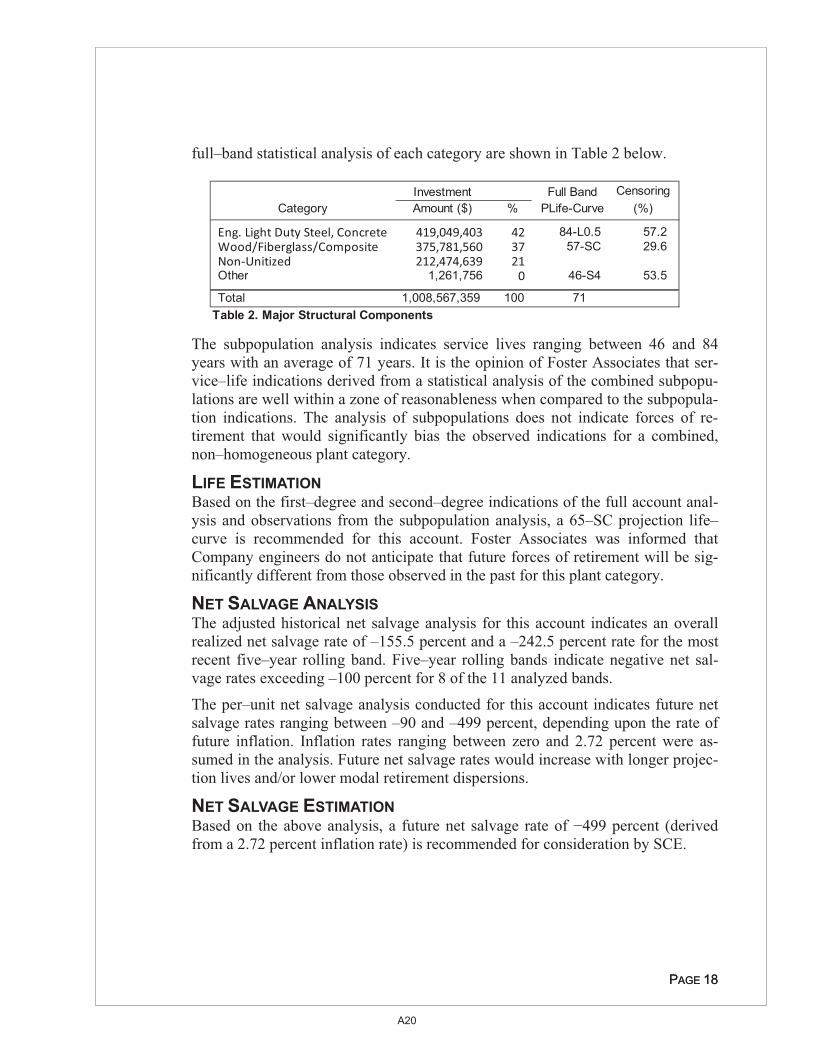
full–band statistical analysis of each category are shown in Table 2 below.

The subpopulation analysis indicates service lives ranging between 46 and 84 years with an average of 71 years. It is the opinion of Foster Associates that ser-vice–life indications derived from a statistical analysis of the combined subpopu-lations are well within a zone of reasonableness when compared to the subpopula-tion indications. The analysis of subpopulations does not indicate forces of re-tirement that would significantly bias the observed indications for a combined, non–homogeneous plant category.

LIFE ESTIMATION Based on the first–degree and second–degree indications of the full account anal-ysis and observations from the subpopulation analysis, a 65–SC projection life–curve is recommended for this account. Foster Associates was informed that Company engineers do not anticipate that future forces of retirement will be sig-nificantly different from those observed in the past for this plant category.

NET SALVAGE ANALYSIS The adjusted historical net salvage analysis for this account indicates an overall realized net salvage rate of –155.5 percent and a –242.5 percent rate for the most recent five–year rolling band. Five–year rolling bands indicate negative net sal-vage rates exceeding –100 percent for 8 of the 11 analyzed bands.


NET SALVAGE ESTIMATION Based on the above analysis, a future net salvage rate of �499 percent (derived from a 2.72 percent inflation rate) is recommended for consideration by SCE.

�

��

PAGE 18PAGE 18


Eng.�Light�Duty�Steel,�Concrete 419,049,403�� 42�� 84-L0.5 57.2 Wood/Fiberglass/Composite 375,781,560�� 37�� 57-SC 29.6 Non�Unitized 212,474,639�� 21��Other 1,261,756 0�� 46-S4 53.5


A20

TRANSMISSION PLANT ACCOUNT: 356.00 – OVERHEAD CONDUCTORS AND DEVICES DESCRIPTION This account includes the installed cost of overhead conductors and devices used for transmission purposes. Account statistics and current and proposed parameters are shown in Table 1 below.

LIFE ANALYSIS Forces of retirement acting upon transmission conductors include deterioration re-sulting from atmospheric corrosion, fatigue failure due to conductor vibration, storm damage, failure of splices or dead–ends, relocation (e.g., highway widen-ing, damsite construction, etc.), circuit upgrades, system reconfiguration and idle facilities (e.g., closure of generation facilities or loss of large customers).

The statistical service life analysis for this account indicates average service lives exceeding 85 years. The analysis, however, is based on $18M of retirement activi-ty from derived additions exceeding $1.5B. Retirement activity of 1.2 percent of derived additions is not considered sufficient to provide a reliable basis for service life estimation.

The composition of major categories (or subpopulations) of plant classified in this account at December 31, 2015 is shown in Table 2. More than 40 percent of the classified investment is conductor larger than 1500 MCM. Service life indications obtained from a full–band statistical analysis of the major categories are shown in Table 2 below.

�

PAGE 19

��


Conductor > 220 kV 739,015,019 50 106-R3 57.7 Conductor < 220 kV 202,769,129 14 82-R1.5 84.0 Switches 27,761,688 2 39-R1 2.5 Non-Unitized 399,410,246 27 Other 113,151,541 8 199-SQ 100.0


Investment

A21

The subpopulation analysis of the full historical experience evidences a range of average service lives between 39 and 199 years with a dollar–weighted average of 110 years. These indications are compromised by high censoring and minimal re-tirement activity comparable to observations in the full account.

LIFE ESTIMATION With consideration given to the minimal retirement experience in this account and the resulting extremes in service life indications, Foster Associates deferred to the Company in recommending retention of the currently approved 61–R3 projection service–life parameters.

NET SALVAGE ANALYSIS The adjusted historical net salvage analysis for this account indicates an overall net salvage rate of –284.3 percent. However, as noted above, this history is based on relatively minimal retirement activity over the period 2002–2015.



.

�

�

PAGE 20

�

A22

TRANSMISSION PLANT ACCOUNT: 357.00 – UNDERGROUND CONDUIT DESCRIPTION This account includes the installed cost of underground conduit and tunnels used for housing transmission cables or wires. Account statistics and current and pro-posed parameters are shown in Table 1.

LIFE ANALYSIS Rebuild and digging are the major forces of retirement expected to affect this ac-count. The statistical service–life analysis for the full account is based on highly censored trials (87 percent) with life indications ranging between 88 and 146 years. Only $387,297 or 0.6% of derived additions has been retired from the ac-count.

The composition of major categories (or subpopulations) of plant classified in this account at December 31, 2015 and the service life indications obtained from a

full–band statistical analysis of each category are shown in Table 2 below.

Subpopulation service life indications are similarly derived from highly censored trials providing little insight into future live expectancies.

�

PAGE 21


Conduit 34,334,761 56 130-S1.5 86.3 Manholes and Vaults 17,239,213 28 65-S2 81.1 Trenches 2,063,079 3 N/ANon-unitized 7,410,219 12 Other 39,791 0 N/A


Investment

Current ProposedPlife-Curve 55-R3 55-R3Future NS Rate 0.0% 0.0%Realized NS -69.5%Average Age (yrs.) 15.6Derived Additions $61,474,359Plant Retirements $387,297Percent Retired 0.6%Plant Balance $61,087,062


A23

LIFE ESTIMATION Neither the full account nor the subpopulation analysis is considered to provide sufficient evidence to support adjusting the currently approved 55–R3 projection life and curve. Current parameters are, therefore, recommended to be retained for this account.

NET SALVAGE ANALYSIS The adjusted net salvage analysis for this account indicates an overall net salvage rate of –69.5% percent realized from minimal retirement activity of only $387,297.

NET SALVAGE ESTIMATION The historical net salvage experience is considered insufficient to support an ad-justment to the currently approved zero percent future net salvage rate. The cur-rent rate is, therefore, recommended for consideration by SCE.

�

PAGE 22

A24

TRANSMISSION PLANT ACCOUNT: 358.00 – UNDERGROUND CONDUCTORS AND DEVICES DESCRIPTION This account includes the installed cost of underground conductors and devices used for transmission purposes. Account statistics and current and proposed pa-rameters are shown in Table 1 below.

LIFE ANALYSIS Deterioration, failure, relocations, upgrades and accidental dig–ins are the major forces of retirement acting upon underground conductors. The statistical life anal-ysis conducted for this account indicates average service lives between the mid–30s and mid–40s for trials with lower censoring, conformance indexes, and non–negative retirement ratios.


An analysis of the subpopulations indicates a range of service lives between 29 and 45 years with lower modal dispersions and an average of 41 years. Service–life indications derived from a statistical analysis of the combined subpopulations are well within a zone of reasonableness when compared to the subpopulation in-

�

PAGE 23


Conductor 163,955,728 61 45-S1.5 51.1 Potheads 27,568,689 10 29-S2 5.2 Arresters 19,845,390 7 31-S1.5 2.0 Cathodic Protection 12,086,839 4 39-R1 81.4 Non-unitized 45,155,677 17


Current ProposedPlife-Curve 40-R2.5 45-S1Future NS Rate -15.0% -25.0%Realized NS -27.0%Average Age (yrs.) 11.6Derived Additions $284,995,149Plant Retirements $16,382,826Percent Retired 6.1%Plant Balance $268,612,323


A25

dications. The analysis of subpopulations does not indicate forces of retirement that would significantly bias the observed indications for a combined, nonhomo-geneous plant category.

LIFE ESTIMATION Based on these observations and considerations, a 45–S1 projection life–curve is recommended for this account. Foster Associates was informed that Company en-gineers do not anticipate that future forces of retirement will be significantly dif-ferent from those observed in the past for this plant category.

NET SALVAGE ANALYSIS The adjusted historical net salvage analysis for this account indicates an overall net salvage rate of –27 percent realized from $16M of retirement activity over the period 2002–2015. Five–year rolling bands are relatively stable and range be-tween –14.4 and –49.7 percent. The most recent 5–year rolling band indicates a realized average net salvage rate of –30.6 percent.

NET SALVAGE ESTIMATION Based on the analysis observations, a –25 percent future net salvage rate is rec-ommended for consideration by SCE. Consideration was given in this recommen-dation to both the –27 historical average realized net salvage rate and the likeli-hood of more negative future net salvage given recent experience such as the –30.6 percent realized net salvage rate observed for the most recent 5–year rolling band.

�

PAGE 24

A26

TRANSMISSION PLANT ACCOUNT: 359.00 – ROADS AND TRAILS DESCRIPTION This account includes the cost of roads, trails, and bridges used primarily as transmission facilities. Account statistics and current and proposed parameters are shown in Table 1 below.

LIFE ANALYSIS The statistical service life analysis for this account is based on minimal retirement activity of $154,514, or 0.1 percent of derived additions from an average plant balance exceeding $108M over the period 2002–2015. Retirements were reported in only 3 years during that period. The service life analysis is highly censored at more than 76.8 percent with resulting life indications ranging between 95 and 175 years.

LIFE ESTIMATION Statistical service life indications for this account are considered insufficient to warrant an adjustment to the currently approved projection life. The current SQ projection curve, however, is considered extreme given the historical experience and the likelihood of more dispersed retirements. Based on these observations and considerations, a 60–R5 projection life–curve is recommended for this account.

NET SALVAGE ANALYSIS The adjusted historical net salvage analysis for this account indicates a realized net salvage rate of –314.1 percent from retirements recorded in 2010, 2012, and 2013 only.

NET SALVAGE ESTIMATION The underlying retirement experience in the historical net salvage analysis is not considered sufficient to warrant adjusting the currently approved zero percent fu-ture net salvage. Retention of the current rate is, therefore, recommended for con-sideration by SCE.

�

PAGE 25

Current ProposedPlife-Curve 60-SQ 60-R5Future NS Rate 0.0% 0.0%Realized NS -314.1%Average Age (yrs.) 5.1Derived Additions $194,172,555Plant Retirements $154,514Percent Retired 0.1%Plant Balance $194,018,041


A27

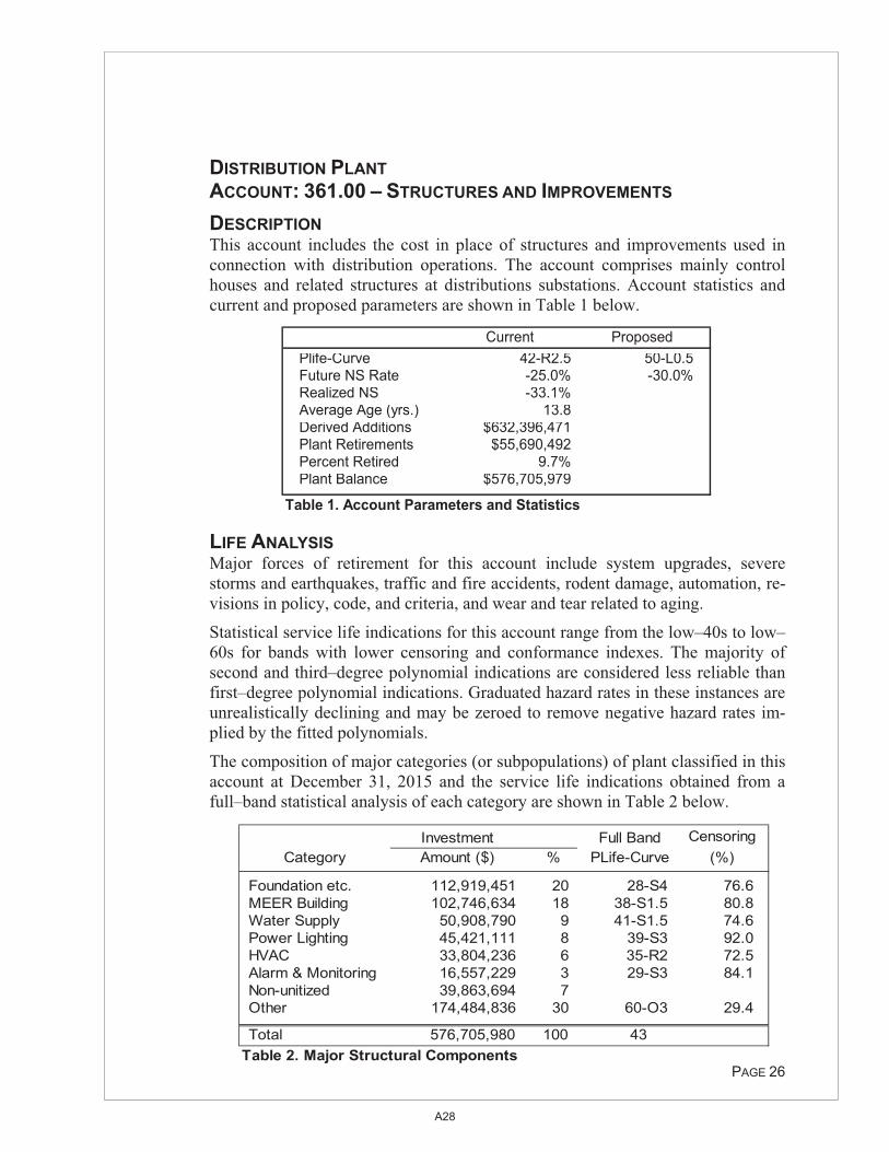
DISTRIBUTION PLANT ACCOUNT: 361.00 – STRUCTURES AND IMPROVEMENTS DESCRIPTION This account includes the cost in place of structures and improvements used in connection with distribution operations. The account comprises mainly control houses and related structures at distributions substations. Account statistics and current and proposed parameters are shown in Table 1 below.

LIFE ANALYSIS Major forces of retirement for this account include system upgrades, severe storms and earthquakes, traffic and fire accidents, rodent damage, automation, re-visions in policy, code, and criteria, and wear and tear related to aging.

Statistical service life indications for this account range from the low–40s to low–60s for bands with lower censoring and conformance indexes. The majority of second and third–degree polynomial indications are considered less reliable than first–degree polynomial indications. Graduated hazard rates in these instances are unrealistically declining and may be zeroed to remove negative hazard rates im-plied by the fitted polynomials.


�

PAGE 26


Foundation etc. 112,919,451 20 28-S4 76.6 MEER Building 102,746,634 18 38-S1.5 80.8 Water Supply 50,908,790 9 41-S1.5 74.6 Power Lighting 45,421,111 8 39-S3 92.0 HVAC 33,804,236 6 35-R2 72.5 Alarm & Monitoring 16,557,229 3 29-S3 84.1 Non-unitized 39,863,694 7 Other 174,484,836 30 60-O3 29.4


Current ProposedPlife-Curve 42-R2.5 50-L0.5Future NS Rate -25.0% -30.0%Realized NS -33.1%Average Age (yrs.) 13.8Derived Additions $632,396,471Plant Retirements $55,690,492Percent Retired 9.7%Plant Balance $576,705,979


A28

An analysis of the subpopulations indicates average service lives ranging between 29 and 60 years, various dispersions, and a dollar–weighted mean of 43 years.

LIFE ESTIMATION Based on these observations and ignoring origin–modal dispersions in which chance is a more pervasive force of retirement, a 50–L0.5 projection life–curve is recommended for this account.

Service–life indications derived from a statistical analysis of the combined sub-populations are well within a zone of reasonableness when compared to the sub-population indications. The analysis of subpopulations does not indicate forces of retirement that would significantly bias the observed indications for a combined, nonhomogeneous plant category. Company operations personnel do not expect policy or procedural changes or technological advances that would introduce sig-nificantly different forces of retirement from those observed in the past.

NET SALVAGE ANALYSIS The historical net salvage analysis for this account indicates an adjusted overall net salvage rate of –33.1 percent realized from $55,690,492 of retirement activity over the period 2002–2015. Five–year rolling band rates have not been less nega-tive than –21.3 percent during that period and the five–year band ending in in 2015 shows a –44.2 percent net salvage rate.

NET SALVAGE ESTIMATION Based on these observations and considerations, a –30 percent future net salvage rate is recommended for consideration by SCE. It is considered unlikely that the upward trend in cost of removal will reverse in the near future.

�

PAGE 27

A29

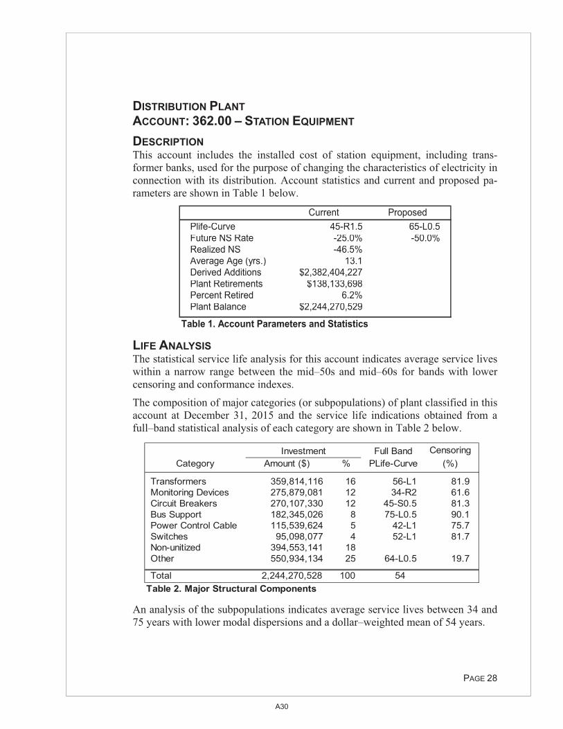
DISTRIBUTION PLANT ACCOUNT: 362.00 – STATION EQUIPMENT DESCRIPTION This account includes the installed cost of station equipment, including trans-former banks, used for the purpose of changing the characteristics of electricity in connection with its distribution. Account statistics and current and proposed pa-rameters are shown in Table 1 below.

LIFE ANALYSIS The statistical service life analysis for this account indicates average service lives within a narrow range between the mid–50s and mid–60s for bands with lower censoring and conformance indexes.


An analysis of the subpopulations indicates average service lives between 34 and 75 years with lower modal dispersions and a dollar–weighted mean of 54 years.

�

PAGE 28


Transformers 359,814,116 16 56-L1 81.9 Monitoring Devices 275,879,081 12 34-R2 61.6 Circuit Breakers 270,107,330 12 45-S0.5 81.3 Bus Support 182,345,026 8 75-L0.5 90.1 Power Control Cable 115,539,624 5 42-L1 75.7 Switches 95,098,077 4 52-L1 81.7 Non-unitized 394,553,141 18 Other 550,934,134 25 64-L0.5 19.7


Investment

Current ProposedPlife-Curve 45-R1.5 65-L0.5Future NS Rate -25.0% -50.0%Realized NS -46.5%Average Age (yrs.) 13.1Derived Additions $2,382,404,227Plant Retirements $138,133,698Percent Retired 6.2%Plant Balance $2,244,270,529


A30

Service–life indications derived from a statistical analysis of the combined sub-populations are well within a zone of reasonableness when compared to the sub-population indications. The analysis of subpopulations does not indicate forces of retirement that would significantly bias the observed indications for a combined, nonhomogeneous plant category.

LIFE ESTIMATION Based on these observations and considerations, a 65–L0.5 projection life–curve is recommended for this account. This recommendation is within the range of both full account and subpopulation service life indications. Foster Associates was informed that Company engineers do not anticipate that future forces of re-tirement will be significantly different from those observed in the past for this plant category.

Although not equivalent to dollar–years of service, SCE engineers estimate a mean time to wear–out of about 37 years for A–Bank (200 kV) transformers and about 57 years for B–Bank (115 or 66 kV) transformers. The number of trans-formers in service at year–end 2015 was 158 A–Bank and 2,226 B–Bank. Com-pany engineers also estimate that the mean time to wear–out of mainline and radi-al oil switches is about 35 years and about 49 years for circuit breakers. The aver-age age of transformers measured in unit�years is about 26 years whereas the av-erage age measured in dollar–years is about 10 years. Similarly, the average age of circuit breakers measured in unit�years is about 32 years whereas the average age measured in dollar–years is about 10 years.

NET SALVAGE ANALYSIS The adjusted historical net salvage analysis for this account indicates an overall net salvage rate of –46.5 percent, realized from $138,133,698 of retirement activi-ty and 5.8 percent of derived addition over the period 2002–2015. Most recent 5–year rolling bands ending in 2013, 2014,and 2015 exhibit net salvage rates of –47.2, –65.6 and –81.4 percent respectively.

NET SALVAGE ESTIMATION Based on these observations and the expectation of continuing negative net sal-vage, a –50 percent future net salvage rate is recommended for consideration by SCE.

PAGE 29

�

A31

DISTRIBUTION PLANT ACCOUNT: 364.00 – POLES, TOWERS AND FIXTURES DESCRIPTION This account includes the installed cost of poles, towers, and related fixtures used for supporting overhead distribution conductors and service wires. Account sta-tistics and current and proposed parameters are shown in Table 1 below.

LIFE ANALYSIS The majority of wood poles in the Company's system are full–length and "through–boring" treated to protect against decay and insect attack. Wood poles may also be treated with a steel stub or a fiberglass wrap to provide additional support. In addition to pole treatment, the Company conducts a 10–year inspec-tion cycle to address safety and reliability. Tree trimming and vegetation man-agement are also a significant component of reliability measures undertaken by the Company.

As with transmission wood poles, major forces of retirement acting upon distribu-tion wood poles include external, internal, top rot, split top deterioration and pole loading. Additional forces include vehicles, wind, storm, fire, and bird (mainly woodpecker) damage. Response to these forces partly depends on the specific lo-cale of the pole given the Company's wide geographical area encompassing main-ly desert but also agricultural, rural, and urban communities.

The statistical service life analysis for this account indicates consistent indications with average service lives around the mid–50s for bands with lower censoring and conformance indexes.


An analysis of the single subpopulation of poles indicates a 53–R1 projection life–curve at 46 percent censoring. This indication is comparable to indications obtained for the full band statistical service life analysis.

�

PAGE 30

A32

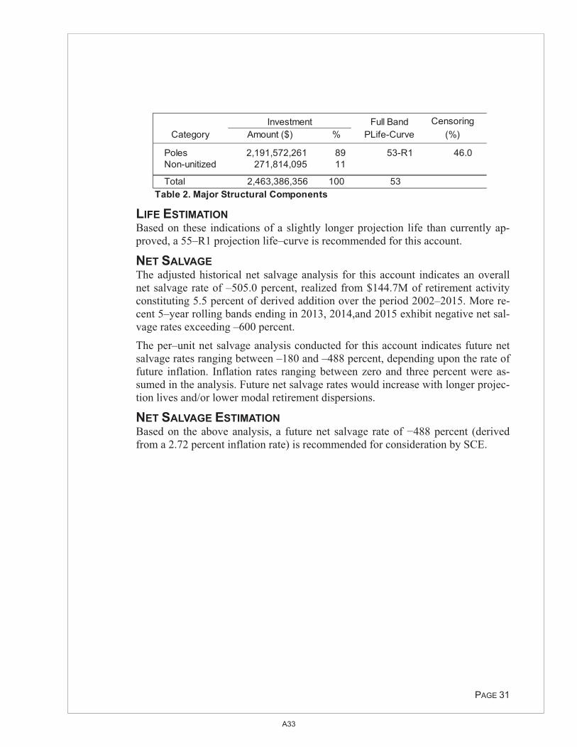
LIFE ESTIMATION Based on these indications of a slightly longer projection life than currently ap-proved, a 55–R1 projection life–curve is recommended for this account.

NET SALVAGE The adjusted historical net salvage analysis for this account indicates an overall net salvage rate of –505.0 percent, realized from $144.7M of retirement activity constituting 5.5 percent of derived addition over the period 2002–2015. More re-cent 5–year rolling bands ending in 2013, 2014,and 2015 exhibit negative net sal-vage rates exceeding –600 percent.

The per–unit net salvage analysis conducted for this account indicates future net salvage rates ranging between –180 and –488 percent, depending upon the rate of future inflation. Inflation rates ranging between zero and three percent were as-sumed in the analysis. Future net salvage rates would increase with longer projec-tion lives and/or lower modal retirement dispersions.


�

�

PAGE 31


Poles 2,191,572,261 89 53-R1 46.0 Non-unitized 271,814,095 11


Investment

A33

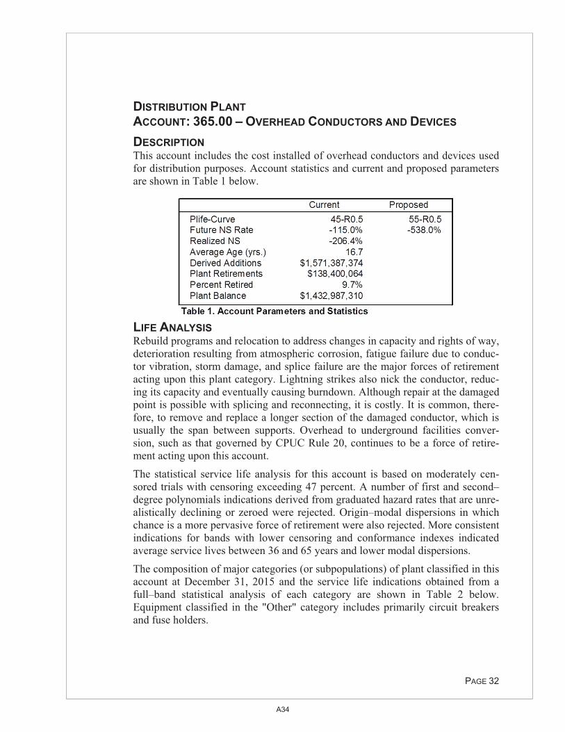
DISTRIBUTION PLANT ACCOUNT: 365.00 – OVERHEAD CONDUCTORS AND DEVICES DESCRIPTION This account includes the cost installed of overhead conductors and devices used for distribution purposes. Account statistics and current and proposed parameters are shown in Table 1 below.

LIFE ANALYSIS Rebuild programs and relocation to address changes in capacity and rights of way, deterioration resulting from atmospheric corrosion, fatigue failure due to conduc-tor vibration, storm damage, and splice failure are the major forces of retirement acting upon this plant category. Lightning strikes also nick the conductor, reduc-ing its capacity and eventually causing burndown. Although repair at the damaged point is possible with splicing and reconnecting, it is costly. It is common, there-fore, to remove and replace a longer section of the damaged conductor, which is usually the span between supports. Overhead to underground facilities conver-sion, such as that governed by CPUC Rule 20, continues to be a force of retire-ment acting upon this account.

The statistical service life analysis for this account is based on moderately cen-sored trials with censoring exceeding 47 percent. A number of first and second–degree polynomials indications derived from graduated hazard rates that are unre-alistically declining or zeroed were rejected. Origin–modal dispersions in which chance is a more pervasive force of retirement were also rejected. More consistent indications for bands with lower censoring and conformance indexes indicated average service lives between 36 and 65 years and lower modal dispersions.

The composition of major categories (or subpopulations) of plant classified in this account at December 31, 2015 and the service life indications obtained from a full–band statistical analysis of each category are shown in Table 2 below. Equipment classified in the "Other" category includes primarily circuit breakers and fuse holders.

�

PAGE 32

A34

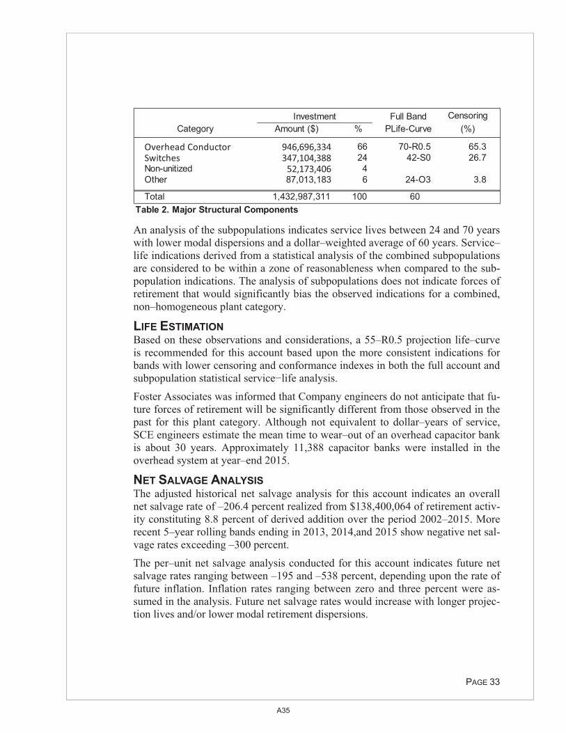
An analysis of the subpopulations indicates service lives between 24 and 70 years with lower modal dispersions and a dollar–weighted average of 60 years. Service–life indications derived from a statistical analysis of the combined subpopulations are considered to be within a zone of reasonableness when compared to the sub-population indications. The analysis of subpopulations does not indicate forces of retirement that would significantly bias the observed indications for a combined, non–homogeneous plant category.

LIFE ESTIMATION Based on these observations and considerations, a 55–R0.5 projection life–curve is recommended for this account based upon the more consistent indications for bands with lower censoring and conformance indexes in both the full account and subpopulation statistical service�life analysis.

Foster Associates was informed that Company engineers do not anticipate that fu-ture forces of retirement will be significantly different from those observed in the past for this plant category. Although not equivalent to dollar–years of service, SCE engineers estimate the mean time to wear–out of an overhead capacitor bank is about 30 years. Approximately 11,388 capacitor banks were installed in the overhead system at year–end 2015.

NET SALVAGE ANALYSIS The adjusted historical net salvage analysis for this account indicates an overall net salvage rate of –206.4 percent realized from $138,400,064 of retirement activ-ity constituting 8.8 percent of derived addition over the period 2002–2015. More recent 5–year rolling bands ending in 2013, 2014,and 2015 show negative net sal-vage rates exceeding –300 percent.

The per–unit net salvage analysis conducted for this account indicates future net salvage rates ranging between –195 and –538 percent, depending upon the rate of future inflation. Inflation rates ranging between zero and three percent were as-sumed in the analysis. Future net salvage rates would increase with longer projec-tion lives and/or lower modal retirement dispersions.

�

PAGE 33


Overhead�Conductor 946,696,334�� 66 70-R0.5 65.3 Switches 347,104,388�� 24 42-S0 26.7 Non-unitized 52,173,406�� 4 Other 87,013,183 6 24-O3 3.8


Investment

A35


PAGE 34

�

A36

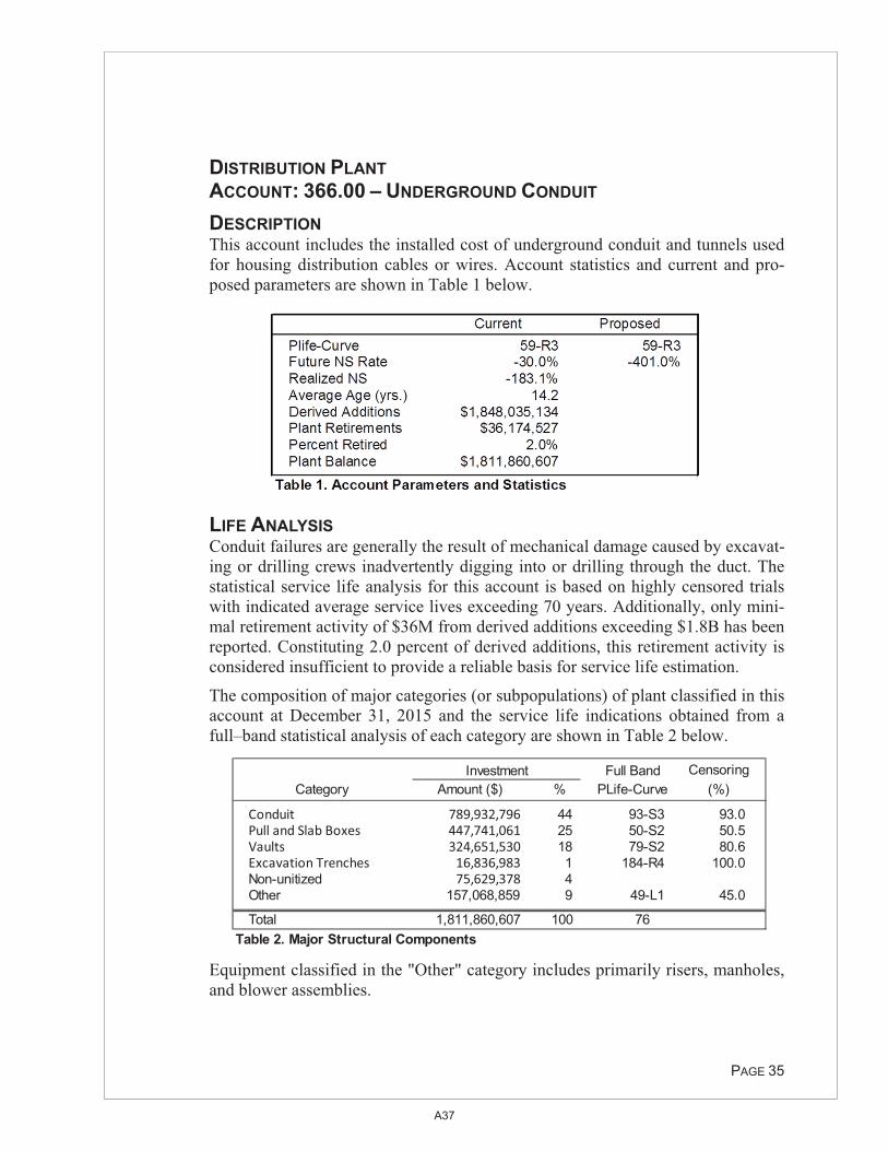
DISTRIBUTION PLANT ACCOUNT: 366.00 – UNDERGROUND CONDUIT DESCRIPTION This account includes the installed cost of underground conduit and tunnels used for housing distribution cables or wires. Account statistics and current and pro-posed parameters are shown in Table 1 below.

LIFE ANALYSIS Conduit failures are generally the result of mechanical damage caused by excavat-ing or drilling crews inadvertently digging into or drilling through the duct. The statistical service life analysis for this account is based on highly censored trials with indicated average service lives exceeding 70 years. Additionally, only mini-mal retirement activity of $36M from derived additions exceeding $1.8B has been reported. Constituting 2.0 percent of derived additions, this retirement activity is considered insufficient to provide a reliable basis for service life estimation.


Equipment classified in the "Other" category includes primarily risers, manholes, and blower assemblies.

�

PAGE 35


Conduit 789,932,796�� 44 93-S3 93.0 Pull�and�Slab�Boxes 447,741,061�� 25 50-S2 50.5 Vaults 324,651,530�� 18 79-S2 80.6 Excavation�Trenches 16,836,983�� 1 184-R4 100.0 Non-unitized 75,629,378�� 4 Other 157,068,859 9 49-L1 45.0


Investment

A37

As noted with the full account analysis, high censoring of the subpopulations also produces indeterminate service life indications.

LIFE ESTIMATION With consideration given to the minimal retirement experience in this account and the resulting unreliable service–life indications, Foster Associates deferred to the Company in recommending retention of the currently approved 59–R3 projection service–life parameters.

NET SALVAGE ANALYSIS The adjusted historical net salvage analysis for this account indicates an overall net salvage rate of –183.1 percent. As noted above, however, this history provides minimal retirement activity over the period 2002–2015.

The per–unit net salvage analysis conducted for this account indicates future net salvage rates ranging between –108 and –401 percent, depending upon the rate of future inflation. Inflation rates ranging between zero and 2.72 percent were as-sumed in the analysis. Future net salvage rates would increase with longer projec-tion lives and/or lower modal retirement dispersions..


�

�

PAGE 36

A38

DISTRIBUTION PLANT ACCOUNT: 367.00 – UNDERGROUND CONDUCTORS AND DEVICES DESCRIPTION This account includes the installed cost of underground conductors and devices used for distribution purposes. Account statistics and current and proposed pa-rameters are shown in Table 1 below.

LIFE ANALYSIS The majority of SCE’s underground cable population is XLPE, which generally fails due to breakdown of insulation over time. The statistical service life analysis for this account indicates average service lives in a narrow range between 40.5 and 44.7 years with lower modal dispersions for trials with lower censoring, con-formance indexes, and hazard functions not compromised by negative or declin-ing rates.


Equipment classified in the "Other" category includes primarily circuit breakers and switches.

An analysis of the subpopulations indicates a 27–L1 and a 45–R2 service life curves with lower modal dispersions and a dollar–weighted mean of 42 years. Service–life indications derived from a statistical analysis of the combined sub-

�

PAGE 37


Cable 4,452,641,073 80 45-R2 18.6 Non-unitized 288,856,647 5 Other 809,879,908 15 27-L1 18.1


Investment

A39

populations are considered to be within a zone of reasonableness when compared to the subpopulation indications. The analysis of subpopulations does not indicate forces of retirement that would significantly bias the observed indications for a combined, non–homogeneous plant category.

LIFE ESTIMATION Based on these observations and considerations, a 45–R1.5 projection life–curve is recommended for this account. Foster Associates was informed that Company engineers do not anticipate that future forces of retirement will be significantly different from those observed in the past for this plant category.

Although not equivalent to dollar–years of service, SCE engineers estimate a mean time to failure (MTTF) of 41 years for cross–linked polyethylene (XLPE) and 46 years for tree retardant cross–linked polyethylene (TR–XLPE) conductor. Company engineers also estimate that the mean time to wear–out of underground mainline and radial oil switches is about 35 years and the mean time to wear–out of an underground capacitor bank is about 30 years and 25 years for automatic re-closers. Approximately 11,549 subsurface oil–filled switches, 2,253 capacitor banks and 47 automatic reclosers were installed in the underground system at year–end 2015.

NET SALVAGE ANALYSIS The adjusted historical net salvage analysis for this account indicates an overall net salvage rate of –155.7 percent realized from $398,585,960 of retirement activ-ity constituting 6.7 percent of derived addition over the period 2002–2015. The most recent four 5–year rolling bands show negative net salvage rates exceeding –150 percent.



�

�

PAGE 38

A40

DISTRIBUTION PLANT ACCOUNT: 368.00 – LINE TRANSFORMERS DESCRIPTION This account includes the investment in overhead and underground distribution line transformers used in transforming electric energy to secondary voltages. Equipment continues to be classified in this account regardless of whether actual-ly in service or held in reserve for future use. Account statistics and current and proposed parameters are shown in Table 1 below.

LIFE ANALYSIS Distribution transformers are replaced when they fail in service or when deteriora-tion is observed during inspection or other field work. Deterioration includes leaks, corrosion and damage caused by vehicles or acts of nature. The statistical service life analysis for this account is stable and indicates average service lives in the mid–20s to high–30s and lower modal dispersions for bands with lower cen-soring and conformance indexes. It should be noted, however, that “cradle–to–grave” accounting is used for line transformers and associated equipment (e.g., capacitors and network protectors). Service lives indicated from a statistical anal-ysis provide estimates of the age at which transformers are permanently retired from service.


�

PAGE 39

Investment Full BandCategory Amount ($) % PLife-Curve

Undeground�Transformers 1,262,937,734 36 34-S2Overhead�Transformers 1,045,618,106 30 40-S2Fuseholders 749,306,101�� 21 38-S3Non-unitized 57,769,013 2 Other 393,008,343 11 25-O2


A41

An analysis of the subpopulations indicates average service lives between 25 and 40 years with lower modal dispersions and a dollar–weighted mean of 36 years. Service–life indications derived from a statistical analysis of the combined sub-populations are considered to be within a zone of reasonableness when compared to the subpopulation indications. The analysis of subpopulations does not indicate forces of retirement that would significantly bias the observed indications for a combined, nonhomogeneous plant category.

LIFE ESTIMATION Service–life indications from both the full account and subpopulation polynomial analyses bound the currently approved 33–S1.5 projection life–curve. Adjusting the currently approved parameters would imply a degree of precision beyond that which can be measured or estimated from a statistical life analysis.

Based on these considerations, retention of a 33–S1.5 projection–life is recom-mended for this account.

NET SALVAGE ANALYSIS The adjusted historical net salvage analysis for this account indicates an overall net salvage rate of –46.9 percent realized from $525.8M of retirement activity constituting 13.0 percent of derived addition over the period 2002–2015. Most re-cent 5–year rolling bands show negative net salvage rates exceeding –130 percent.



�

�

PAGE 40

A42

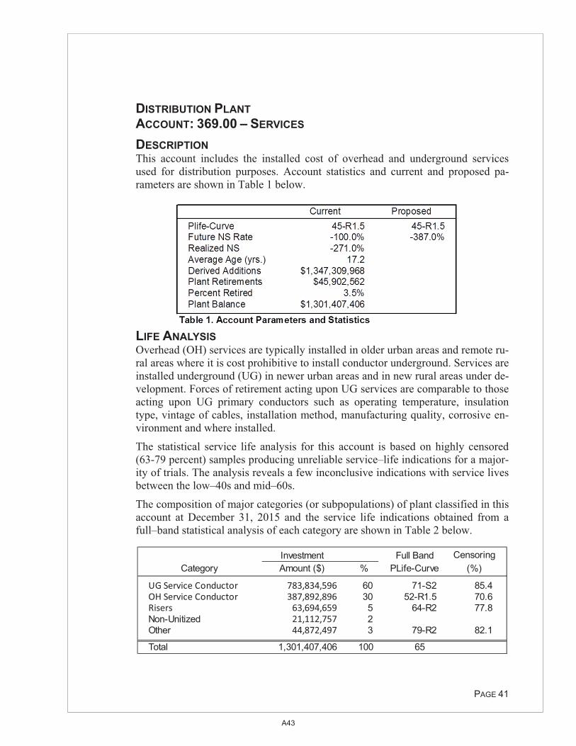
DISTRIBUTION PLANT ACCOUNT: 369.00 – SERVICES DESCRIPTION This account includes the installed cost of overhead and underground services used for distribution purposes. Account statistics and current and proposed pa-rameters are shown in Table 1 below.

LIFE ANALYSIS Overhead (OH) services are typically installed in older urban areas and remote ru-ral areas where it is cost prohibitive to install conductor underground. Services are installed underground (UG) in newer urban areas and in new rural areas under de-velopment. Forces of retirement acting upon UG services are comparable to those acting upon UG primary conductors such as operating temperature, insulation type, vintage of cables, installation method, manufacturing quality, corrosive en-vironment and where installed.

The statistical service life analysis for this account is based on highly censored (63-79 percent) samples producing unreliable service–life indications for a major-ity of trials. The analysis reveals a few inconclusive indications with service lives between the low–40s and mid–60s.


�

PAGE 41


UG�Service�Conductor 783,834,596�� 60 71-S2 85.4 OH�Service�Conductor 387,892,896�� 30 52-R1.5 70.6 Risers 63,694,659�� 5 64-R2 77.8 Non-Unitized 21,112,757�� 2 Other 44,872,497�� 3 79-R2 82.1

Total 1,301,407,406 100 65

A43

Equipment classified in the "Other" category includes primarily underground conduit.

An analysis of the subpopulations indicates full–band average service lives be-tween 52 and 79 years with lower modal dispersions and a dollar–weighted mean of 65 years. Subpopulation service life indications are similarly based on highly censored trials and the resulting indications are considered less than conclusive.

LIFE ESTIMATION Neither the full account nor the subpopulation analysis provides sufficient evi-dence to warrant adjusting the currently approved 45–R1.5 projection life and curve. It was also revealed in conducting the analysis of this account that the pric-ing and vintaging of retirements may be contributing to the observed high degrees of censoring. Pending further investigation of the ageing of retirements, Foster Associates concurs with SCE that current parameters should be retained for this account.

NET SALVAGE ANALYSIS The adjusted historical net salvage analysis for this account indicates an overall net salvage rate of –271.0 percent realized from $45.4M of retirement activity constituting 3.4 percent of derived addition over the period 2002–2015. The most recent three 5–year rolling bands show negative net salvage rates exceeding –500 percent.

The per–unit net salvage analysis conducted for this account indicates future net salvage rates ranging between –178 and –387 percent, depending upon the rate of future inflation. Inflation rates ranging between zero and 2.72 percent were as-sumed in the analysis. Future net salvage rates would increase with longer projec-tion lives and/or lower modal retirement dispersions..


�

�

PAGE 42

A44

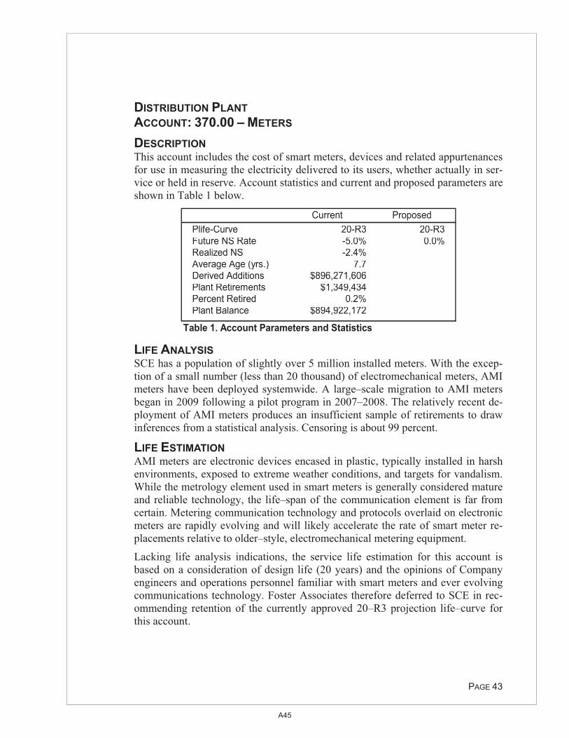
DISTRIBUTION PLANT ACCOUNT: 370.00 – METERS DESCRIPTION This account includes the cost of smart meters, devices and related appurtenances for use in measuring the electricity delivered to its users, whether actually in ser-vice or held in reserve. Account statistics and current and proposed parameters are shown in Table 1 below.

LIFE ANALYSIS SCE has a population of slightly over 5 million installed meters. With the excep-tion of a small number (less than 20 thousand) of electromechanical meters, AMI meters have been deployed systemwide. A large–scale migration to AMI meters began in 2009 following a pilot program in 2007–2008. The relatively recent de-ployment of AMI meters produces an insufficient sample of retirements to draw inferences from a statistical analysis. Censoring is about 99 percent.

LIFE ESTIMATION AMI meters are electronic devices encased in plastic, typically installed in harsh environments, exposed to extreme weather conditions, and targets for vandalism. While the metrology element used in smart meters is generally considered mature and reliable technology, the life–span of the communication element is far from certain. Metering communication technology and protocols overlaid on electronic meters are rapidly evolving and will likely accelerate the rate of smart meter re-placements relative to older–style, electromechanical metering equipment.

Lacking life analysis indications, the service life estimation for this account is based on a consideration of design life (20 years) and the opinions of Company engineers and operations personnel familiar with smart meters and ever evolving communications technology. Foster Associates therefore deferred to SCE in rec-ommending retention of the currently approved 20–R3 projection life–curve for this account.

�

PAGE 43

Current ProposedPlife-Curve 20-R3 20-R3Future NS Rate -5.0% 0.0%Realized NS -2.4%Average Age (yrs.) 7.7Derived Additions $896,271,606Plant Retirements $1,349,434Percent Retired 0.2%Plant Balance $894,922,172


A45

NET SALVAGE ANALYSIS The adjusted historical net salvage analysis for this account is based upon a min-imal amount of $1.3M retired between 2011 and 2015 from derived additions ex-ceeding $896M. The analysis indicates an overall net salvage rate of –271.0 per-cent realized from $45.4M of retirement activity constituting 3.4 percent of de-rived addition over the period 2002–2015. The most recent three 5–year rolling bands indicate negative net salvage rates exceeding –500 percent. The historical net salvage recorded in this account is not considered to be a reasonable predictor of future net salvage for AMI meters.

NET SALVAGE ESTIMATION Noting that “cradle–to–grave” accounting is used for meters and associated equipment (e.g., current and potential transformers), minimal salvage and cost of disposal are expected for this account. Meter removal and reinstallation costs are charged to expense. Based on these observations and expectations, a zero percent future net salvage rate is recommended for consideration by SCE.

�

�

PAGE 44

A46

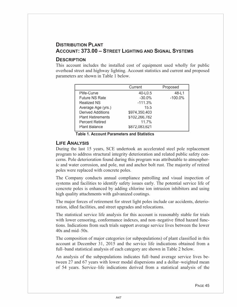
DISTRIBUTION PLANT ACCOUNT: 373.00 – STREET LIGHTING AND SIGNAL SYSTEMS DESCRIPTION This account includes the installed cost of equipment used wholly for public overhead street and highway lighting. Account statistics and current and proposed parameters are shown in Table 1 below.

LIFE ANALYSIS During the last 15 years, SCE undertook an accelerated steel pole replacement program to address structural integrity deterioration and related public safety con-cerns. Pole deterioration found during this program was attributable to atmospher-ic and water corrosion, and pole, nut and anchor bolt rust. The majority of retired poles were replaced with concrete poles.

The Company conducts annual compliance patrolling and visual inspection of systems and facilities to identify safety issues early. The potential service life of concrete poles is enhanced by adding chlorine ion intrusion inhibitors and using high quality attachments with galvanized coatings.

The major forces of retirement for street light poles include car accidents, deterio-ration, idled facilities, and street upgrades and relocations.

The statistical service life analysis for this account is reasonably stable for trials with lower censoring, conformance indexes, and non–negative fitted hazard func-tions. Indications from such trials support average service lives between the lower 40s and mid–50s.


An analysis of the subpopulations indicates full–band average service lives be-tween 27 and 67 years with lower modal dispersions and a dollar–weighted mean of 54 years. Service–life indications derived from a statistical analysis of the

�

PAGE 45

Current ProposedPlife-Curve 40-L0.5 48-L1Future NS Rate -30.0% -100.0%Realized NS -111.3%Average Age (yrs.) 15.5Derived Additions $974,350,403Plant Retirements $102,266,782Percent Retired 11.7%Plant Balance $872,083,621


A47

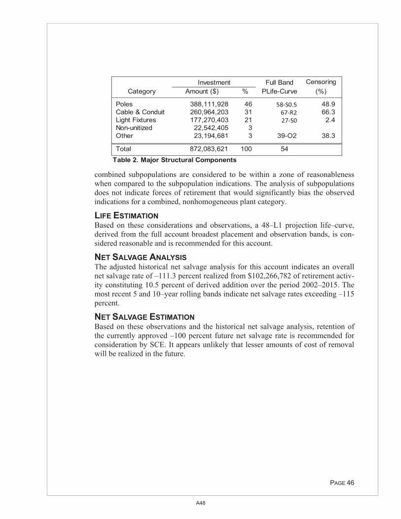
combined subpopulations are considered to be within a zone of reasonableness when compared to the subpopulation indications. The analysis of subpopulations does not indicate forces of retirement that would significantly bias the observed indications for a combined, nonhomogeneous plant category.

LIFE ESTIMATION Based on these considerations and observations, a 48–L1 projection life–curve, derived from the full account broadest placement and observation bands, is con-sidered reasonable and is recommended for this account.

NET SALVAGE ANALYSIS The adjusted historical net salvage analysis for this account indicates an overall net salvage rate of –111.3 percent realized from $102,266,782 of retirement activ-ity constituting 10.5 percent of derived addition over the period 2002–2015. The most recent 5 and 10–year rolling bands indicate net salvage rates exceeding –115 percent.

NET SALVAGE ESTIMATION Based on these observations and the historical net salvage analysis, retention of the currently approved –100 percent future net salvage rate is recommended for consideration by SCE. It appears unlikely that lesser amounts of cost of removal will be realized in the future.

�

�

PAGE 46


Poles 388,111,928 46 58�S0.5 48.9 Cable & Conduit 260,964,203 31 67�R2 66.3 Light Fixtures 177,270,403 21 27�S0 2.4 Non-unitized 22,542,405 3 Other 23,194,681 3 39-O2 38.3

Total 872,083,621 100 54

Table 2. Major Structural Components

Investment

A48

GENERAL PLANT DEPRECIABLE ACCOUNT: 390.00 – STRUCTURES AND IMPROVEMENTS DESCRIPTION This account includes the cost in place of structures and improvements used for Company purposes, the cost of which is not properly includible in other structures and improvements accounts. Account statistics and current and proposed parame-ters are shown in Table 1 and the composition of major structural components classified in this account at December 31, 2015 is shown in Table 2.

LIFE ANALYSIS The statistical service life analysis for this account indicates average service lives between 40 and 60 years for trials with lower censoring and conformance indexes. A number of trials are considered less reliable if hazard rates are unrealistically declining or zeroed to avoid the suggestion of negative hazard rates. No attempt was made to analyze equipment classified in the subpopulations for this plant cat-egory.

�

PAGE 47

InvestmentCategory Amount ($) %

Common 229,531,472 24 Buildings 220,785,582 23 Power & Lighting Systems 170,306,642 18 HVAC 100,134,622 11 Alarms and Monitoring Systems 65,852,228 7 Foundations & Related Structures 57,908,077 6 Water Supply Systems 33,133,484 3 Non-unitized 27,376,214 3 Miscellaneous 42,058,937 4

947,087,257 100

Table 2. Structural Components Distribution

Current ProposedPlife-Curve 38-R3 45-R0.5Future NS Rate -5.0% -10.0%Realized NS -24.5%Average Age (yrs.) 12.7Derived Additions $1,035,908,700Plant Retirements $88,821,443Percent Retired 9.4%Plant Balance $947,087,257


A49

LIFE ESTIMATION Based on the indications obtained from the broader bands of the statistical life analysis, a 45–R0.5 projection life–curve is recommended for this account. Foster Associates was informed that Company engineers do not anticipate that future forces of retirement will be significantly different from those observed in the past for this plant category.

NET SALVAGE ANALYSIS The historical net salvage analysis for this account indicates an overall adjusted net salvage rate of –24.1 percent realized from $88.8M of retirement activity con-stituting 8.6 percent of derived addition over the 2002–2015 study period.

NET SALVAGE ESTIMATION Based on these observations and the expectation of continuing negative net sal-vage, a –10 percent future net salvage rate is recommended for consideration by SCE. This recommendation adjusts the future net salvage parameter from a –5 percent in the direction of the historical net salvage observations.

�

�

PAGE 48

A50

Appendix B

Formulation of Per Unit Net Salvage Rates

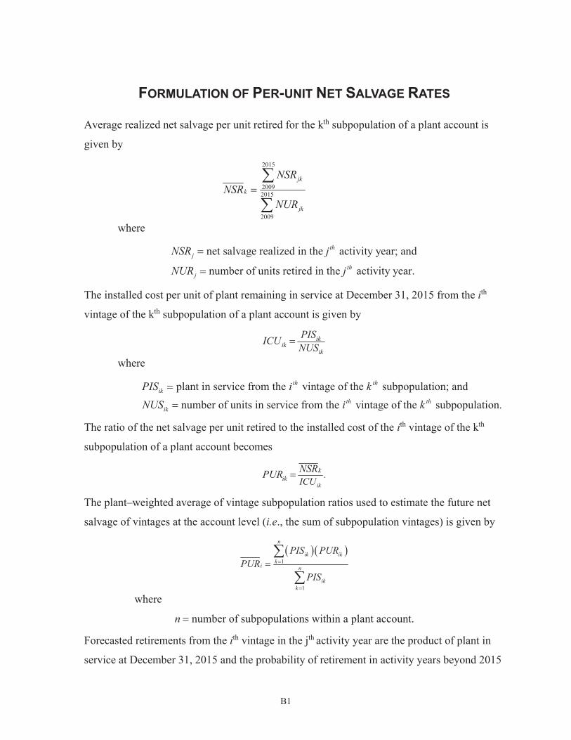
B1

2015

20092015

2009

jk

k

jk

NSRNSR

NUR

FORMULATION OF PER-UNIT NET SALVAGE RATES

Average realized net salvage per unit retired for the kth subpopulation of a plant account is

given by

where

The installed cost per unit of plant remaining in service at December 31, 2015 from the ith

vintage of the kth subpopulation of a plant account is given by

where

The ratio of the net salvage per unit retired to the installed cost of the ith vintage of the kth

subpopulation of a plant account becomes

The plant–weighted average of vintage subpopulation ratios used to estimate the future net

salvage of vintages at the account level (i.e., the sum of subpopulation vintages) is given by

where

Forecasted retirements from the ith vintage in the jth activity year are the product of plant in

service at December 31, 2015 and the probability of retirement in activity years beyond 2015

ikik

ik

PISICUNUS

1

1

n

ik ikk

i n

ikk

PIS PURPUR

PIS

net salvage realized in the activity year; and

number of units retired in the activity year.

thj

thj

NSR j

NUR j

number of subpopulations within a plant account.n

.ik

kik ICU

NSRPUR

plant in service from the vintage of the subpopulation; andnumber of units in service from the vintage of the subpopulation.

th thik

th thik

PIS i kNUS i k

B2

obtained from an Iowa–type probability density function. Retirements from the ith vintage in

the jth activity year are given by

where

ijp = probability of retirement during age interval j–i–0.5 and j–i+0.5.

Estimated future net salvage for retirements from the ith vintage in the jth activity year is given

by

where The estimated future net salvage rate for a plant account is the ratio of the sum of future net

salvage to the sum of vintaged plant in service given by

ij i ijRET PIS p

20151 jiij ijFNS RET PUR r

'

.ij

i j

iki k

FNSFNS

PIS

estimated rate of inflation.r

Documents

Results of Operations Volume 03 – Depreciation Study of Operations Volume 03 – Depreciation Study Before the Public Utilities Commission of the State of California Rosemead, California