Embed Size (px)
Citation preview

Procedia Computer Science 00 (2012) 1–6
Procedia ComputerScience
International Workshop on Cooperative Robots and Sensor Networks (RoboSense)
Restoring Wireless Sensor Network Connectivity in Damaged Environments
Thuy T. Truong, Kenneth N. Brown, Cormac J. Sreenan
Mobile & Internet Systems Laboratory and Cork Constraint Computation Centre, Dept of Computer Science, University College Cork, Ireland
Abstract
A wireless sensor network can become partitioned due to node failure, requiring the deployment of additionalrelay nodes in order to restore network connectivity. This introduces an optimisation problem involving a tradeoff
between the number of additional nodes that are required and the costs of moving through the sensor field for thepurpose of node placement. This tradeoff is application-dependent, influenced for example by the relative urgencyof network restoration. We propose four heuristic algorithms which integrate network design with path planning,recognising the impact of obstacles on mobility and communication. We conduct an empirical evaluation of the fouralgorithms on random connectivity and mobility maps, showing their relative performance in terms of node and pathcosts, and assessing their execution speeds. Finally, we examine how the relative importance of the two objectivesinfluences the choice of algorithm.
Keywords: Wireless Sensor Network, Network Repair, Path Planning, Explorationc©2011 Published by Elsevier Ltd. Selection and/or peer-review under responsibility of [name organizer]
1. Introduction
Wireless Sensor Networks are becoming increasingly important for monitoring phenomena in remote or hazardousenvironments, including pollution monitoring, chemical process sensing, disaster response, and battlefield monitoring.As these environments are uncontrolled and may be volatile, the network may suffer damage, from hazards, directattack or accidental damage from wildlife and weather. They may also degrade through battery depletion or hardwarefailure. The failure of an individual sensor node may mean the loss of particular data streams generated by that node;more significantly, node failure may partition the network, meaning that many data streams cannot be transmitted tothe sink. This creates the network repair problem, in which we must place new radio nodes in the environment torestore connectivity to the sink for all sub-partitions.
There are four main subtasks in the problem: (i) determining what damage has occurred (i.e. which nodes havefailed and what radio links have been blocked); (ii) determining what changes, if any, have happened to the accessibil-ity of the environment (i.e. what positions can be reached, and what routes are possible between those positions); (iii)deciding on the positions for the new radio nodes; and (iv) planning and following a route through the environmentto place those nodes. The problem thus involves both exploration and optimisation, and may require the placement ofnodes before the changes to connectivity and accessibility have been fully mapped. We assume possible locations fornew radio nodes are limited to a finite set of positions where a node can be securely placed and which can be accessed.Radio nodes are expensive, and so solutions which require fewer nodes are preferred. Physically moving around theenvironment may be expensive in energy use, may take significant time, or may expose the agent placing the nodes todanger, and so solutions which allow cheaper path plans are also preferred. Depending on the application, either one

/ Procedia Computer Science 00 (2012) 1–6
of the two objectives may be more important: placing expensive nodes in, for example, agricultural pollution moni-toring favours solutions with fewer nodes, while restoring connectivity during disaster response favours solutions thatcan be deployed quickly even if they require more nodes. Thus the network repair problem is multi-objective.
We introduce the problem of simultaneous network repair and autonomous exploration and route planning in thepresence of unknown obstacles. We assume a set of locations from which sensor data is required by the network, andwe assume the agent has knowledge of the network and accessibility prior to the damage occurring. The objective isto connect as many as possible of these locations, placing extra sensors if required, while minimising the number ofradio nodes and the mobility costs. We consider two different priorities for the multi-objective problem: minimisingmobility costs, and minimisng the number of radio nodes. For each one, we develop a greedy approach and a globalapproach. In each case, the agent computes a plan (or partial plan), and then starts to execute it. When the agentdiscovers new information about accessibility or connectivity, it recomputes the plan from its current location, andthen continues. We evaluate the approaches on randomly generated problems, and analyse their effectiveness underdifferent assumptions.
2. The Network Exploration and Restoration Problem
We assume a rectilinear grid of locations G, in which a subset Gb ⊆ G of grid squares are candidate locationsfor wireless nodes. The centre of each square is a potential position for a wireless node. We assume an agent canmove from a square to one of its 4 rectilinear neighbours, unless that neighbour is blocked. The set of blocked squaresbefore damage is Bb, while the set of blocked squares after damage is Ba, such that Bb ⊆ Ba ⊆ G. We assume a nodecan sense its own square plus neighbouring squares at a distance of Rs, and has a maximum communication range ofRt (e.g. if Rt = 1, then the node can communicate with at most its 8 immediate neighbours). We assume a set of Cb ofpotential radio links, where each potential link can connect two endpoints {gi ∈ Gb, g j ∈ Gb}. After damage, the setof candidate locations is Ga ⊆ Gb and the set of potential links is Ca ⊆ Cb and a set of live nodes is GA ⊆ Ga. Theset τ represents terminals, the squares from which we need sensed data. A set I ⊂ GA of active nodes where it stillhas connection to wider network. We assume the starting location of the agent is at L ∈ I. Figure 1 shows exampleof pre-damage, current and actual maps of the network. At the start of the problem, we assume the agent knows τ, I,L, Bb, Gb, and Cb. As the agent explores the environment, it will maintain: Gk, the locations where it knows nodesare active; Ge, locations where knows no node exists; Ck, the radio links it knows are possible; Ce, the radio links itknows are broken; Bk, the squares it knows to be blocked; S e, squares it knows to be free; and Lk, its own currentlocation.
Pre-damage map Actual map (after the damage) Current map
Notation
UNKNOWN square
BLOCK square
FREE square
Candidate location
Terminal location
Location with an alive node
Location with node placed
Potential radio link Established radio link
Agent’s location
Figure 1: Example network conditions before and after damage.
We assume the agent is able to probe neighbouring squares up to a distance of k, to determine whether or notthey are blocked (but cannot probe a distant neighbour if there is a blocked square inbetween). A probe costs α unitsper square. The agent is able to test a radio link by listening for transmission from an active node. When the agentdiscovers a new live radio node, it will also be told all of that node’s live multi-hop neighbours. There is no cost forlistening for transmissions. The agent can detect whether or not there is a sensor node on its current location, and maydrop a new node at the centre of that square. The cost of moving one square is m, while the cost of placing a node isw. The objective is to connect as many as possible of the squares in τ to I, placing nodes in those squares if necessary,minimising the sum of the mobility costs and the probe costs, and minimising the number of nodes placed.
/ Procedia Computer Science 00 (2012) 1–6
3. Approach
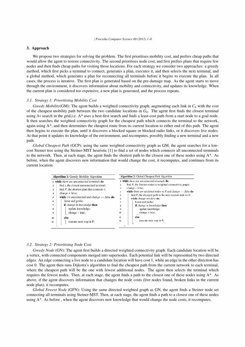
We propose two strategies for solving the problem. The first prioritises mobility cost, and prefers cheap paths thatwould allow the agent to restore connectivity. The second prioritises node cost, and first prefers plans that require fewnodes and then finds cheap paths for visiting those locations. For each strategy we consider two approaches: a greedymethod, which first picks a terminal to connect, generates a plan, executes it, and then selects the next terminal, anda global method, which generates a plan for reconnecting all terminals before it begins to execute the plan. In allcases, the process is iterative. The first plan is generated based on the pre-damage map. As the agent starts to movethrough the environment, it discovers information about mobility and connectivity, and updates its knowledge. Whenthe current plan is considered too expensive, a new plan is generated, and the process repeats.
3.1. Strategy 1: Prioritising Mobility CostGreedy Mobility(GM): The agent builds a weighted connectivity graph, augmenting each link in Cb with the cost
of the cheapest mobility path between the two candidate locations in Gb. The agent first finds the closest terminalusing A∗ search in the grid,i.e. A* uses a best-first search and finds a least-cost path from a start node to a goal node.It then searches the weighted connectivity graph for the cheapest path which connects the terminal to the network,again using A*, and then determines the cheapest route from its current location to either end of this path. The agentthen begins to execute the plan, until it discovers a blocked square or blocked radio links, or it discovers live nodes.At that point it updates its knowledge of the environment, and recomputes, possibly finding a new terminal and a newpath.
Global Cheapest Path (GCP): using the same weighted connectivity graph as GM, the agent searches for a low-cost Stenier tree using the Steiner-MST heuristic [1] to find a set of nodes which connects all unconnected terminalsto the network. Then, at each stage, the agent finds the shortest path to the closest one of these nodes using A*. Asbefore, when the agent discovers new information that would change the cost, it recomputes, and continues from itscurrent location.
3.2. Strategy 2: Prioritising Node CostGreedy Node (GN): The agent first builds a directed weighted connectivity graph. Each candidate location will be
a vertex, with connected components merged into supernodes. Each potential link will be represented by two directededges. An edge connecting a live node to a candidate location will have cost 1, while an edge in the other direction hascost 0. The agent then runs Dijkstra’s algorithm to find the cheapest path from the current network to each terminal,where the cheapest path will be the one with fewest additional nodes. The agent then selects the terminal whichrequires the fewest nodes. Then, at each stage, the agent finds a path to the closest one of these nodes using A*. Asabove, if the agent discovers information that changes the node costs (live nodes found, broken links in the currentnode plan), it recomputes.
Global Fewest Node (GFN): Using the same directed weighted graph as GN, the agent finds a Steiner node setconnecting all terminals using Steiner-MST. Then, at each stage, the agent finds a path to a closest one of these nodesusing A*. As before , when the agent discovers new knowledge that would change the node costs, it recomputes.

/ Procedia Computer Science 00 (2012) 1–6
4. Experiments
The algorithms presented above are heuristic, and take different approaches to a multi-objective problem. There-fore, we evaluate them empirically on randomly generated maps, to compare their runtimes and the quality of theirsolutions for both objectives. We assume a pre-damage grid map consisting of n × m squares each of size 10 units.We randomly select c grid squares to be candidate locations, and g squares to be blocked. For each pair of candidatelocations separated by less than 25 units we allow a potential radio link with probability 0.85. For the map after dam-age, we randomly select a of the candidate locations to be live nodes, and select t candidate locations to be terminals9 (locations for which we require sensor data). We randomly pick b additional squares to be blocked, and remove r%of the radio links. For this paper, we ensure that the problems are feasible - i.e. it is possible for the agent to visit a setof locations where placing nodes would reconnect all the terminals. In each case, the algorithms only probe a squarethat the agent intends to move into. In all experiments, the results are the average of 50 runs at each data point.
First, we consider the effect of varying c,the number of candidates from 40 to 80, while we fix the number ofterminals, t, to 6 and the damage level to < b = 10, r = 10% >. The results are shown in the top row of Fig.2. Thenumber of candidates has little impact on the number of nodes required. However, the mobility costs rise to peakat c = 60: as we increase locations, there are more options to explore, requiring more backtracking on discoveringdamage, until there are enough locations to offer easy alternatives. The runtimes of all heuristics increase with thenumber of candidate locations. GM has the highst runtime, because it is repeatedly forced to recompute on failure.We note that the greedy mobility heuristic has lower mobility cost than the global heuristic, and that the greedy nodeheuristic requiries fewer nodes than the global node heuristic. We believe this is the effect of exploration, as the greedyheuristics are better able to adapt their plans once damage is found.
Secondly, we vary the number of terminals, t, from 4 to 12, while fixing c to 60 and the damage to < 10, 10 >. Theresults are shown in the second row of Fig.2. The number of required nodes increases with the number of terminalsto a peak, but then declines. We believe this decline is because as more terminals are required, more of the area mustbe explored, which reveals more existing live nodes and ultimately simplified the connectivity problem. As expected,the mobility costs continue to rise. Again, GM requires the longest runtime.
Thirdly, we vary the damage level from < 10, 10 > to < 40, 40 >, fixing the candidate locations at 60 and thenumber of terminals at 6. Varying the damage has little impact on the number of new nodes required, but the mobilitycosts rise to a peak and then fall, as there are fewer deep dead ends for the agent to explore.
Finally, we note that the mobility costs are associated only with the distance travelled. For real scenarios, there isa tradeoff between the speed at which connectivity is restored and the cost of the extra nodes. We assume that it takesthe agent 30s to position a new node. We then consider two scenarios, one representing a small robot which movesat 0.1ms−1, and the second representing a larger vehicle moving over rough terrain at 4ms−1. We fix the size of thegrid quare to be 10m × 10m. The total time to restore the network is thus time to place the new nodes plus the time tomove along the path plus the computation time. The results are shown in Fig.3. We can see that for the slow agent,prioritising mobility cost is most important, with the gain in reduced movement from GM more than compensating forthe increased runtime; alternatively, for the faster agent, prioritising the numder of nodes gives a faster repair, sincethe time to place the new nodes outweights the mobility costs. Thus the WSN restoration problem is subtle, with the

/ Procedia Computer Science 00 (2012) 1–6
0
1
2
3
4
5
6
7
8
9
40 50 60 70 80
Required nodes with different number of candidate locations
GM
GN
GCP
GFN
17
19
21
23
25
27
29
31
40 50 60 70 80
nu
mb
er
of
mo
ves
Mobility costs with different number of candidate locations
GM
GN
GCP
GFN
0
1
2
3
4
5
6
40 50 60 70 80
run
tim
e (s
)
Runtime with different number of candidate locations
GM
GN
GCP
GFN
0
2
4
6
8
10
12
14
4 6 8 10 12
Required nodes with different number of terminals
GM
GN
GCP
GFN
15
20
25
30
35
40
45
50
4 6 8 10 12
nu
mb
er
of
mo
ves
Mobility costs with different number of terminals
GM
GN
GCP
GFN
0
0.5
1
1.5
2
2.5
3
3.5
4
4.5
4 6 8 10 12
run
tim
me
(s)
Runtime with different number of terminals
GM
GN
GCP
GFN
0
1
2
3
4
5
6
7
8
9
10
<15,15%> <20,20%> <25,25%> <30,30%> <35,35%> <40,40%>
Required nodes with different level of damage
GM
GN
GCP
GFN 20
22
24
26
28
30
32
34
36
nu
mb
er
of
mo
ves
Mobility costs with different level of damage
GM
GN
GCP
GFN 0
0.5
1
1.5
2
2.5
3
3.5
4
run
tim
e (s
)
Runtime with different level of damage
GM
GN
GCP
GFN
Figure 2: The effect of varying the number of candidate locations, terminals and damage level.
2000
2200
2400
2600
2800
3000
3200
40 50 60 70 80
Total restoring time with different number of candidate locations. V=0.1ms-1
GM
GN
GCP
GFN
1700
2200
2700
3200
3700
4200
4700
5200
4 6 8 10 12
Total restoring time with different number of terminals. V=0.1ms-1
GM
GN
GCP
GFN
2200
2400
2600
2800
3000
3200
3400
3600
3800
<15,15%><20,20%> <25,25%> <30,30%> <35,35%> <40,40%>
Total restoring time with different damage level. V=0.1ms-1
GM
GN
GCP
GFN
240
250
260
270
280
290
300
310
320
40 50 60 70 80
Total restoring time with different number of candidate locations. V=4ms-1
GM
GN
GCP
GFN
200
250
300
350
400
450
500
4 6 8 10 12
Total restoring time with different number of terminals. V=4ms-1
GM
GN
GCP
GFN
265
275
285
295
305
315
325
335
345
<15,15%> <20,20%> <25,25%> <30,30%> <35,35%> <40,40%>
Total restoring time with different damage level. V=4ms-1
GM
GN
GCP
GFN
Figure 3: The effect of different agent speeds
choice of approach clearly dependent on the details of the specific problem. Solution methods must take into accountthe main objectives (minimising infrastructure and minimise time), but also consider the capabilities of the agent thatwill implement the eventual solution.
5. Related Work
The subject of network restoration for wireless sensor networks has been an active area of research. The differentapproaches can be classified as (i) deploying redundant nodes so as to be able to cope with a pre-determined number

/ Procedia Computer Science 00 (2012) 1–6
of failures, (ii) use of mobile (actor) nodes that can be moved into position in order to restore connectivity, (iii) dis-patching mobile nodes in a pre-emptive manner to avoid failures in connectivity, and (iv) the deployment of additionalnodes to restore connectivity after failures have occurred. The latter work is closest to our research but is differentin two respects, firstly in that we optimise both the number of additional nodes as well as the path length needed fortheir deployment, and secondly in that we explicitly take into account the impact of obstacles that can alter both theavailable paths and the ability of nodes to communicate directly. We now provide a summary of the related papers.
In [2],[3] the goal is to deploy k-1 redundant nodes with the intention of achieving k-connectivity, for example byplacing nodes at the intersection between the communication range of each pair of nodes. The number of additionalnodes required by these approaches is prohibitive. Several papers consider the use of mobile actor nodes in networkrestoration, e.g. [4], [5], [6],[7]. The papers propose different strategies to choose the moving actors, for example,based on estimating the shortest moving distance and/or degree of connectivity. The solution space is limited, focusedon dealing with a single failure and re-connecting just two networks at a time, and with an assumption that mobilityis unimpeded by obstacles. [8] proactively deploys additional helper mobile nodes, controlling their trajectories inresponse to predicted network disconnection events. The work assumes that the mobile nodes are always fast enoughto reach the desired destination in case of a predicted disconnection event, and that a full map of the physical terrainand radio environment is available. Details of how to determine the number of mobile nodes that are needed andthe related path planning are not provided. [9] and [10] assume multiple simultaneous failures involving many failednodes and a network that is partitioned into many segments. The approach is to re-connect those segments in acentralized manner with the main objective of using the smallest number of additional nodes. [9] uses a spider webapproach to reconnect the segments while [10] forms a connectivity chain from each segment toward a centre pointand then seeks to optimize the number of additional nodes that are needed.
6. Conclusion
We have defined the new problem of simultaneous network repair and autonomous exploration and route planningin the presence of unknown obstacles. We represent the problem as a multi-objective problem of minimising thenumber of required nodes and mobility costs. We present two strategies, prioritising mobility costs andprioritisingthe number of nodes, and for each we develop two heuristic approaches, one greedy and one with a global view.In all cases, the agent computes a plan based on some initial knowledge and begins to execute it. As it moves, itdiscovers more knowledge of the environemnt, and modifies its plan as required. We evaluate the approaches insimulation, assessing the impact of increasing damage, increasing nodes to be connected, and increasing locationsfor radio nodes. In addition, we show that different agent speeds have a significant impact on performance, and mustbe taken into account when selecting the algorithm. In future work we will explore a wider range of environments,consider continually spreading damage, and investigate the use of teams of agents working in parallel.
Acknowledgment
This work is part of the Irish Higher Education Authority PRTLIIV funded NEMBES project.[1] B. Y. Wu, K.-M. Chao, Spanning Trees and Optimization Problems, Chapman & Hall / CRC Press, USA, 2004.[2] B. Khelifa, H. Haffaf, M. Merabti, D. Llewellyn-Jones, Monitoring connectivity in wireless sensor networks., in: ISCC, IEEE, 2009.[3] H. M. Almasaeid, A. E. Kamal, On the minimum k-connectivity repair in wireless sensor networks., in: ICC, IEEE, 2009, pp. 1–5.[4] K. Akkaya, F. Senel, Detecting and connecting disjoint sub-networks in wireless sensor and actor networks, Ad Hoc Netw. 7.[5] A. Abbasi, M. Younis, U. Baroudi, Restoring connectivity in wireless sensor-actor networks with minimal topology changes, in: Communi-
cations (ICC), 2010 IEEE International Conference on, 2010, pp. 1 –5.[6] K. Akkaya, F. Senel, A. Thimmapuram, S. Uludag, Distributed recovery from network partitioning in movable sensor/actor networks via
controlled mobility, IEEE Trans. Comput. 59 (2010) 258–271.[7] M. Sir, I. Senturk, E. Sisikoglu, K. Akkaya, An optimization-based approach for connecting partitioned mobile sensor/actuator networks, in:
Computer Communications Workshops (INFOCOM WKSHPS), 2011 IEEE Conference on, 2011, pp. 525 –530.[8] L. Dai, V. Chan, Helper node trajectory control for connection assurance in proactive mobile wireless networks, in: Computer Communica-
tions and Networks, 2007. ICCCN 2007. Proceedings of 16th International Conference on, 2007, pp. 882 –887.[9] F. Senel, M. Younis, K. Akkaya, A robust relay node placement heuristic for structurally damaged wireless sensor networks, in: Local
Computer Networks, 2009. LCN 2009. IEEE 34th Conference on, 2009, pp. 633 –640.[10] S. Lee, M. Younis, Recovery from multiple simultaneous failures in wireless sensor networks using minimum steiner tree, Journal of Parallel
Distributed Computing 70 (2010) 525–536.