Restoration for Weakly Blurred and Strongly Noisy Images

Xiang Zhu and Peyman Milanfar

Electrical Engineering Department, University of California, Santa Cruz, CA 95064

xzhu@soe.ucsc.edu, milanfar@ee.ucsc.edu

Abstract

In this paper we present an adaptive sharpening algo-

rithm for restoration of an image which has been corrupted

by mild blur, and strong noise. Most existing adaptive

sharpening algorithms can not handle strong noise well due

to the intrinsic contradiction between sharpening and de-

noising. To solve this problem we propose an algorithm that

is capable of capturing local image structure and sharp-

ness, and adjusting sharpening accordingly so that it effec-

tively combines denoising and sharpening together without

either noise magnification or over-sharpening artifacts. It

also uses structure information from the luminance channel

to remove artifacts in the chrominance channels. Experi-

ments illustrate that compared with other sharpening ap-

proaches, our method can produce state of the art results

under practical imaging conditions.

1. Introduction

Blur and noise are the two common problems that ex-

ist in digital imaging. An important camera setting that

strongly affects these two distortions, and that needs to be

carefully adjusted, is the aperture size. If the exposure time

is fixed, a large aperture will increase the signal to noise

ratio (SNR), meanwhile reducing the depth of field (DOF)

and thus increasing the out-of-focus blur, which eliminates

high-frequency components of the image. On the other

hand, a small aperture will alleviate the blur but increase

the noise level [17, 4]. Noise can also be suppressed by

using longer exposure time; but of course, this may cause

motion (either camera motion or object motion) blur that

is even more difficult to remove [3, 14, 1]. At the same

time, limited accuracy of auto-focus systems and low light

condition may add extra blur and noise into the image. So

in real applications, such as consumer digital imaging, it is

very common to record weakly blurred and relatively noisy

images (see Fig. 6 (a)).

In general, there are two possible types of techniques that

can enhance the sharpness of an image under such condi-

tions. One group of methods is blind-deconvolution. In

recent years, several blind-deconvolution algorithms have

been proposed to restore images degraded by blur [3, 13, 5].

These algorithms are generally designed under the assump-

tion that the point spread function (PSF) of blur is spatially

invariant, and that noise is very weak or virtually absent.

Unfortunately, even when dealing with weakly blurred im-

ages, the presence of noise can be a significant problem

for the state of the art deblurring algorithms. Consider the

popular algorithms under the maximum a-posteriori (MAP)

estimation framework, where total variation (TV) or other

sparse image priors are frequently used [8, 13]. These reg-

ularization terms concentrate on smoothing pixels with me-

dian or small gradient values, leaving high-value gradients

preserved. They perform as smoothing filter assuming a

global model for the locally treated pixels without consider-

ing local image characteristics. Although they can provide

a good balance between high frequency content restoration

and noise suppression, the noise effect may still remain in

the output data, and corrupt the smoothness of latent ob-

ject structure. On the other hand, space invariance of the

PSF does not hold in general for out-of-focus blur since the

scene depth varies spatially [7]. Besides, high computa-

tional cost is another significant shortcoming of deblurring

approaches [2].

Another group of techniques aiming at recovering

weakly blurred images are the sharpening algorithms. The

classic linear unsharp masking (UM) approach, which en-

hances certain high-frequency components of the input im-

age, is popular in practice due to its simplicity. However,

linear unsharp masking is very sensitive to noise and can

easily produce overshoot artifacts [11]. Several adaptive

versions of unsharp masking have been proposed to alle-

viate these problems [11, 12, 6, 18, 2]. In [11] the scaling

factor that controls sharpening strength is determined ac-

cording to local image characteristics measured by ”image

activity”. In smooth and high-contrast areas, the scaling

factors are reduced to avoid noise magnification or over-

sharpening artifacts. The problem for such algorithms is

that they do not effectively suppress existing noise, while

the image activity measure is also sensitive to local noise

variation. So their performance is quite limited when the in-

103978-1-4244-9497-2/10/$26.00 ©2010 IEEE

put noise is strong. The algorithm proposed in [2] incorpo-

rates a denoising filter to smooth the input image, and em-

ploys a clipping process to remove overshoot. However, this

method smooths mostly low-frequency components of the

input image, and enhances unfiltered high-frequency com-

ponent directly, which again amplifies noise. Meanwhile

the clipping process may affect structure smoothness gen-

erating artifacts especially for heavily noisy regions. An-

other sharpening algorithm called adaptive bilateral filter

(ABF) can achieve good noise suppression [18]. ABF was

designed by introducing an offset into the bilateral filter,

which switches the behavior of the filter from denoising to

edge sharpening according to local image structure. This

method focuses on enhancing the the slope of edges, but

its sharpening strength for texture or other image details is

limited.

In this paper a new non-parametric approach called geo-

metric locally adaptive sharpening (GLAS) is proposed for

weakly blurred and strongly noisy images. The algorithm

is derived from local adaptive regression [15]. The key idea

behind this approach is sharpening according to the local

image structure, so that denoising and sharpening processes

can be effectively combined together. Overshoot artifacts

are avoided by adjusting the local sharpening parameter ac-

cording to a robust sharpness measure. Besides, the pro-

posed method is also capable of removing structured color

artifacts caused by, for example, the demosaicing process.

The paper is organized as follows: In Section 2 we motivate

and describe the proposed approach. Section 3 illustrates

the restoration results for real images, and finally Section 4

provides the conclusion.

2. Proposed algorithm

In this section, we first propose an approach called geo-

metric locally adaptive sharpening (GLAS). This approach

takes local image structure into consideration, so that it

can efficiently combine sharpening and denoising together.

Then, the steering kernel (SK) regression technique for im-

age reconstruction [15] is briefly introduced, which is able

to capture local image structure even with presence of mild

blur and strong noise. Based on the SK, a specific algo-

rithm for constructing GLAS kernels for weakly blurred

gray-scale image restoration is developed. Finally we ex-

tend this approach to color images with a strategy for re-

moving chrominance artifacts.

2.1. Motivation

We model the process that degrades an ideal sharp image

f (denoted in a lexicographically ordered vector) into the

observed blurry and noisy data g as:

g = Hf + n (1)

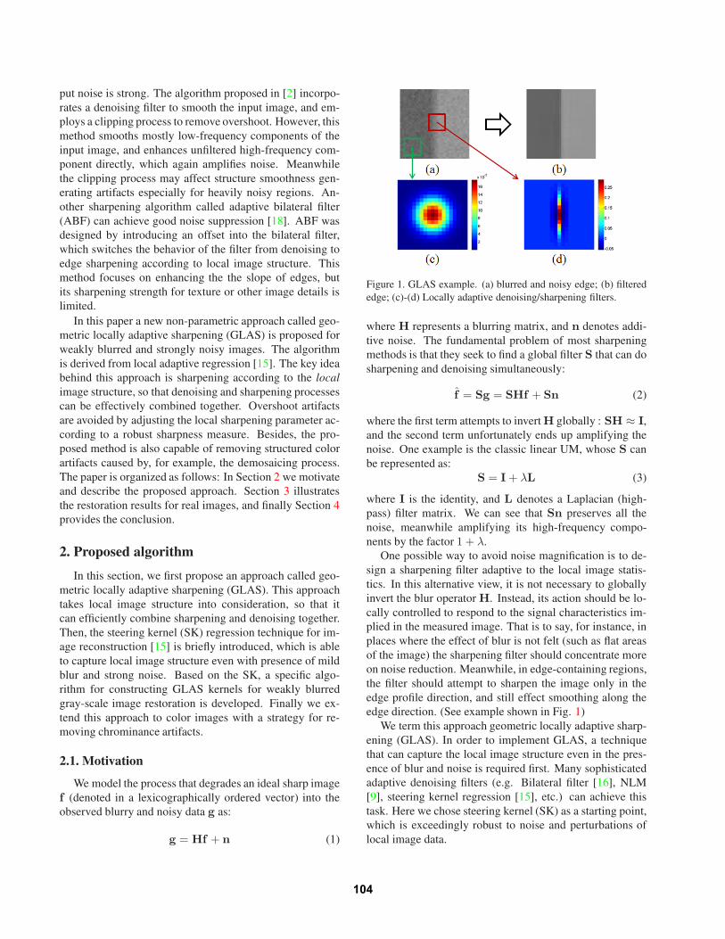
Figure 1. GLAS example. (a) blurred and noisy edge; (b) filtered

edge; (c)-(d) Locally adaptive denoising/sharpening filters.

where H represents a blurring matrix, and n denotes addi-

tive noise. The fundamental problem of most sharpening

methods is that they seek to find a global filter S that can do

sharpening and denoising simultaneously:

f = Sg = SHf + Sn (2)

where the first term attempts to invert H globally : SH ≈ I,

and the second term unfortunately ends up amplifying the

noise. One example is the classic linear UM, whose S can

be represented as:

S = I + λL (3)

where I is the identity, and L denotes a Laplacian (high-

pass) filter matrix. We can see that Sn preserves all the

noise, meanwhile amplifying its high-frequency compo-

nents by the factor 1 + λ.

One possible way to avoid noise magnification is to de-

sign a sharpening filter adaptive to the local image statis-

tics. In this alternative view, it is not necessary to globally

invert the blur operator H. Instead, its action should be lo-

cally controlled to respond to the signal characteristics im-

plied in the measured image. That is to say, for instance, in

places where the effect of blur is not felt (such as flat areas

of the image) the sharpening filter should concentrate more

on noise reduction. Meanwhile, in edge-containing regions,

the filter should attempt to sharpen the image only in the

edge profile direction, and still effect smoothing along the

edge direction. (See example shown in Fig. 1)

We term this approach geometric locally adaptive sharp-

ening (GLAS). In order to implement GLAS, a technique

that can capture the local image structure even in the pres-

ence of blur and noise is required first. Many sophisticated

adaptive denoising filters (e.g. Bilateral filter [16], NLM

[9], steering kernel regression [15], etc.) can achieve this

task. Here we chose steering kernel (SK) as a starting point,

which is exceedingly robust to noise and perturbations of

local image data.

104

2.2. Steering kernel construction

The key idea behind SK is to robustly obtain the local

structure of images by analyzing estimated gradients, and

use this structure information to determine the shape and

size of a canonical kernel [15]. In earlier work, SK has

been successfully utilized to address the image denoising

problem.

Assuming a pixel of interest is located at position xi =[xi, yi], its SK is mathematically represented as:

K(xl − xi) =√

det(Cl) exp{

−(xl − xi)T Cl(xl − xi)

}

(4)

where xl denotes a given location inside the SK window

centered at xi, and Cl is a covariance matrix estimated

from a collection of gradients within an analysis window

wl around xl (more on this below).

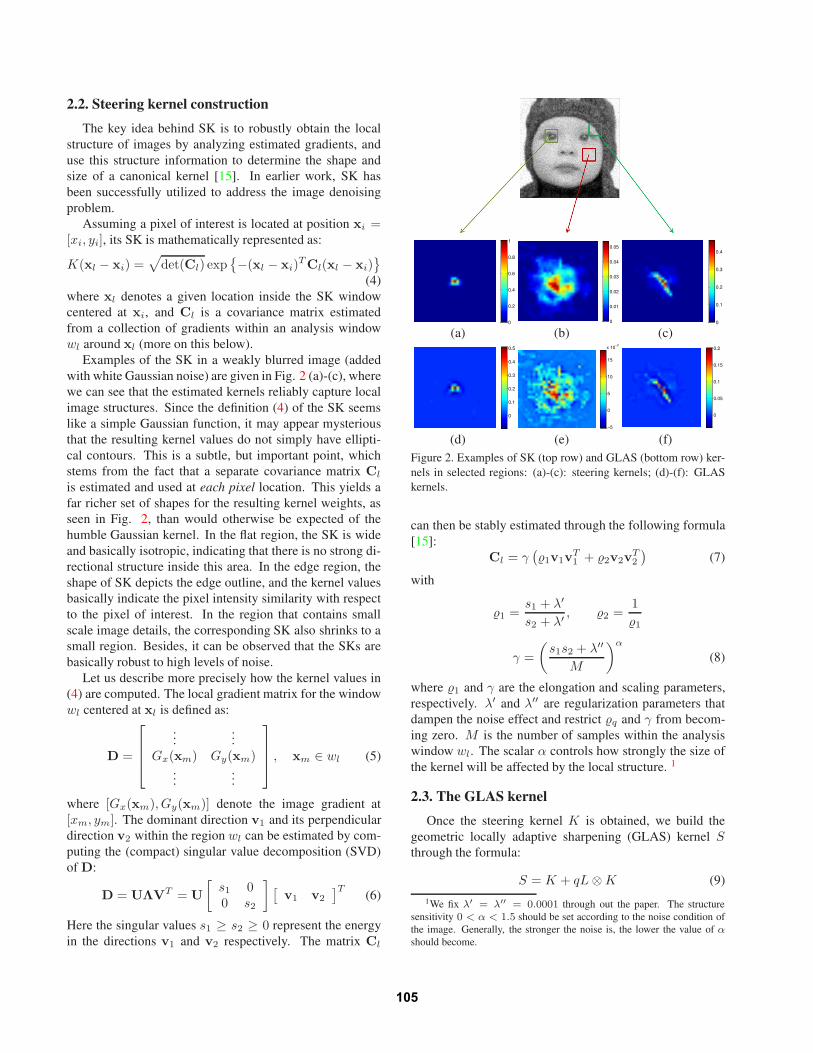
Examples of the SK in a weakly blurred image (added

with white Gaussian noise) are given in Fig. 2 (a)-(c), where

we can see that the estimated kernels reliably capture local

image structures. Since the definition (4) of the SK seems

like a simple Gaussian function, it may appear mysterious

that the resulting kernel values do not simply have ellipti-

cal contours. This is a subtle, but important point, which

stems from the fact that a separate covariance matrix Cl

is estimated and used at each pixel location. This yields a

far richer set of shapes for the resulting kernel weights, as

seen in Fig. 2, than would otherwise be expected of the

humble Gaussian kernel. In the flat region, the SK is wide

and basically isotropic, indicating that there is no strong di-

rectional structure inside this area. In the edge region, the

shape of SK depicts the edge outline, and the kernel values

basically indicate the pixel intensity similarity with respect

to the pixel of interest. In the region that contains small

scale image details, the corresponding SK also shrinks to a

small region. Besides, it can be observed that the SKs are

basically robust to high levels of noise.

Let us describe more precisely how the kernel values in

(4) are computed. The local gradient matrix for the window

wl centered at xl is defined as:

D =

......

Gx(xm) Gy(xm)...

...

, xm ∈ wl (5)

where [Gx(xm), Gy(xm)] denote the image gradient at

[xm, ym]. The dominant direction v1 and its perpendicular

direction v2 within the region wl can be estimated by com-

puting the (compact) singular value decomposition (SVD)

of D:

D = UΛVT = U

[

s1 00 s2

]

[

v1 v2

]T(6)

Here the singular values s1 ≥ s2 ≥ 0 represent the energy

in the directions v1 and v2 respectively. The matrix Cl

0

0.2

0.4

0.6

0.8

1

0

0.01

0.02

0.03

0.04

0.05

0

0.1

0.2

0.3

0.4

(a) (b) (c)

0

0.1

0.2

0.3

0.4

0.5

−5

0

5

10

15

x 10−3

0

0.05

0.1

0.15

0.2

(d) (e) (f)

Figure 2. Examples of SK (top row) and GLAS (bottom row) ker-

nels in selected regions: (a)-(c): steering kernels; (d)-(f): GLAS

kernels.

can then be stably estimated through the following formula

[15]:

Cl = γ(

1v1vT1

+ 2v2vT2

)

(7)

with

1 =s1 + λ′

s2 + λ′, 2 =

1

1

γ =

(

s1s2 + λ′′

M

)α

(8)

where 1 and γ are the elongation and scaling parameters,

respectively. λ′ and λ′′ are regularization parameters that

dampen the noise effect and restrict q and γ from becom-

ing zero. M is the number of samples within the analysis

window wl. The scalar α controls how strongly the size of

the kernel will be affected by the local structure. 1

2.3. The GLAS kernel

Once the steering kernel K is obtained, we build the

geometric locally adaptive sharpening (GLAS) kernel Sthrough the formula:

S = K + qL ⊗ K (9)

1We fix λ′= λ′′

= 0.0001 through out the paper. The structure

sensitivity 0 < α < 1.5 should be set according to the noise condition of

the image. Generally, the stronger the noise is, the lower the value of α

should become.

105

where ⊗ represents the convolution operator, and L denotes

a Laplacian filter. The positive scalar q determines the de-

gree of sharpening (more on this below). The restored im-

age is then computed as a local regression (weighted aver-

age) with the kernel S as follows:

f(xi) =

∑

x∈wlS(x − xi)g(x)

∑

x∈wlS(x − xi)

, (10)

where g is the measured blurry and noisy image. Fig. 2 (d)-

(f) illustrate examples of GLAS kernels. Consider the edge

pixel for instance. The negative values appearing along the

two sides of the edge outline indicate that the sharpening ef-

fect happens in the direction perpendicular to the edge ori-

entation. Meanwhile, we have most positive values along

the outline of the edge, which means the kernel smooths

(denoises) the edge simultaneously. On the other hand, in

the flat region, though there exist few small negative values

across the region, the kernel can still be viewed largely as a

smoothing filter.

One problem that frequently arises in practice, in part

due to limited depth of field of cameras, is that the de-

gree of blur varies in space. As a result, with a globally

designed sharpening approach, some regions that happen

to be already in-focus may be over-sharpened, resulting in

overshoots or ringing artifacts. Without additional finesse,

similar problems could plague the proposed method. If the

local region is already in focus, a fixed, and unnecessarily

high value of q would produce overshoots along the edge

pixels. To alleviate this problem, we next make the sharp-

ening parameter q adaptive to the sharpness of local image

content.

An image sharpness metric, which can estimate the local

image blur even in the presence of noise [20, 19], is imple-

mented here. The metric is based on the singular values of

local gradient matrix, which have already been calculated in

the SK construction stage, so it does not require much extra

calculation. The local metric Q for the pixel located at xl is

defined as [20, 19]:

Q = s1

s1 − s2

s1 + s2

(11)

where s1, s2 were introduced in (6). The blurrier the local

patch of the image is, the lower the Q value becomes.

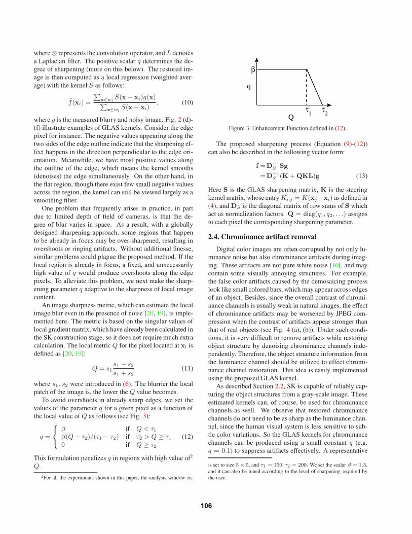
To avoid overshoots in already sharp edges, we set the

values of the parameter q for a given pixel as a function of

the local value of Q as follows (see Fig. 3):

q =

β if Q < τ1

β(Q − τ2)/(τ1 − τ2) if τ2 > Q ≥ τ1

0 if Q ≥ τ2

(12)

This formulation penalizes q in regions with high value of2

Q.

2For all the experiments shown in this paper, the analysis window wl

τ1

τ2

β

q

Q

Figure 3. Enhancement Function defined in (12).

The proposed sharpening process (Equation (9)-(12))

can also be described in the following vector form:

f =D−1

S Sg

=D−1

S (K + QKL)g (13)

Here S is the GLAS sharpening matrix, K is the steering

kernel matrix, whose entry Ki,j = K(xj−xi) as defined in

(4), and DS is the diagonal matrix of row sums of S which

act as normalization factors. Q = diag(q1, q2, . . .) assigns

to each pixel the corresponding sharpening parameter.

2.4. Chrominance artifact removal

Digital color images are often corrupted by not only lu-

minance noise but also chrominance artifacts during imag-

ing. These artifacts are not pure white noise [10], and may

contain some visually annoying structures. For example,

the false color artifacts caused by the demosaicing process

look like small colored bars, which may appear across edges

of an object. Besides, since the overall contrast of chromi-

nance channels is usually weak in natural images, the effect

of chrominance artifacts may be worsened by JPEG com-

pression when the contrast of artifacts appear stronger than

that of real objects (see Fig. 4 (a), (b)). Under such condi-

tions, it is very difficult to remove artifacts while restoring

object structure by denoising chrominance channels inde-

pendently. Therefore, the object structure information from

the luminance channel should be utilized to effect chromi-

nance channel restoration. This idea is easily implemented

using the proposed GLAS kernel.

As described Section 2.2, SK is capable of reliably cap-

turing the object structures from a gray-scale image. These

estimated kernels can, of course, be used for chrominance

channels as well. We observe that restored chrominance

channels do not need to be as sharp as the luminance chan-

nel, since the human visual system is less sensitive to sub-

tle color variations. So the GLAS kernels for chrominance

channels can be produced using a small constant q (e.g.

q = 0.1) to suppress artifacts effectively. A representative

is set to size 5 × 5, and τ1 = 150, τ2 = 200. We set the scalar β = 1.5,

and it can also be tuned according to the level of sharpening required by

the user.

106

example is given in Fig. 4, where it can be seen that the

proposed strategy successfully suppressed basically all the

artifacts (including structured artifacts), meanwhile recon-

structing high-frequency content rather well in chrominance

channels.

To summarize, the overall algorithm can be described as

follows:

Algorithm 1 Algorithm for Color Image Restoration

1. Given an RGB image g, transform it into Y CbCr for-

mat: {gY , gCb, gCr}, and estimate steering kernel K and

local sharpness metric Q at each pixel of the luminance

channel gY .

2. Construct GLAS kernels for the luminance channel

with a spatially adaptive q according to local blurriness Qthrough (9) and (12), and restore the luminance channel

to get fY using (10).

3. Construct GLAS kernels for the luminance channel

with a small constant q, and apply these to restore fCb,

fCr through (10).

4. Combine fY , fCb, fCr to obtain the estimated RGBimage f .

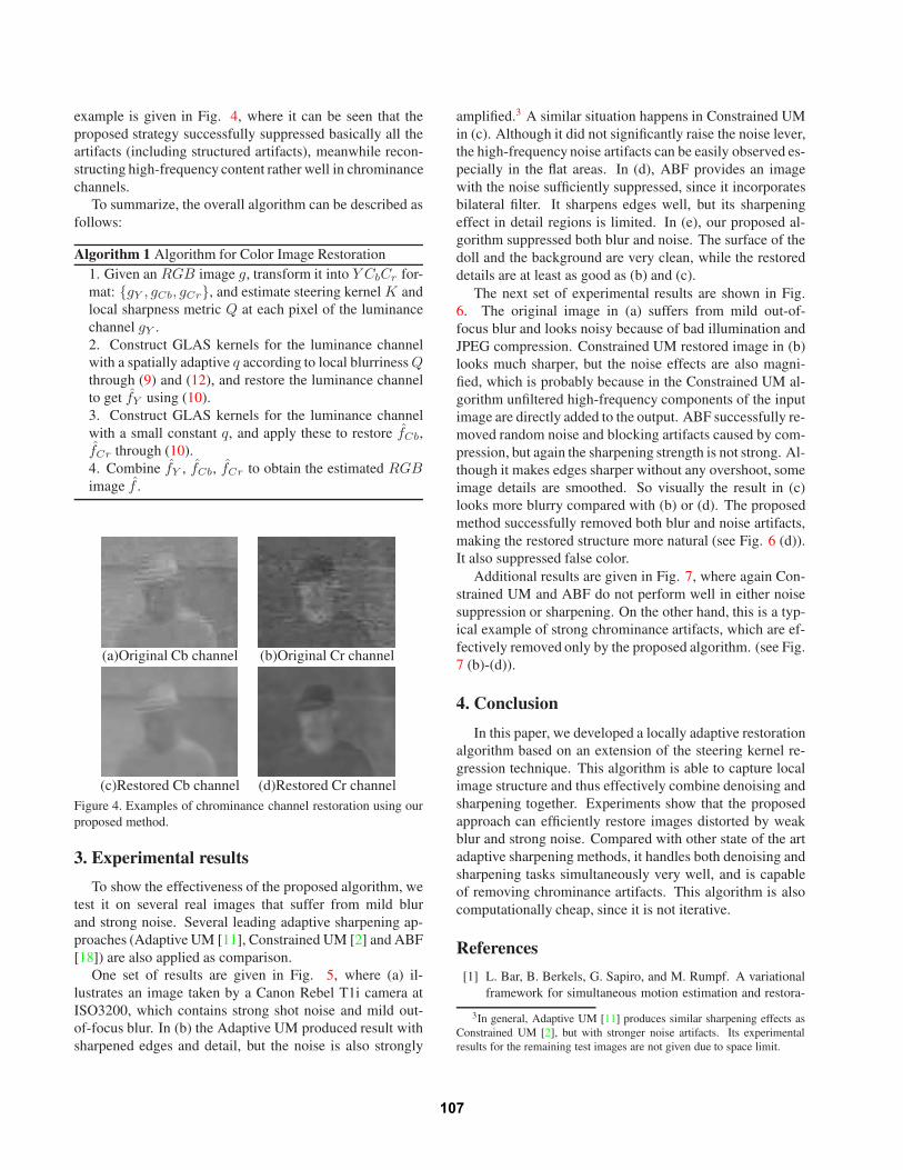
(a)Original Cb channel (b)Original Cr channel

(c)Restored Cb channel (d)Restored Cr channel

Figure 4. Examples of chrominance channel restoration using our

proposed method.

3. Experimental results

To show the effectiveness of the proposed algorithm, we

test it on several real images that suffer from mild blur

and strong noise. Several leading adaptive sharpening ap-

proaches (Adaptive UM [11], Constrained UM [2] and ABF

[18]) are also applied as comparison.

One set of results are given in Fig. 5, where (a) il-

lustrates an image taken by a Canon Rebel T1i camera at

ISO3200, which contains strong shot noise and mild out-

of-focus blur. In (b) the Adaptive UM produced result with

sharpened edges and detail, but the noise is also strongly

amplified.3 A similar situation happens in Constrained UM

in (c). Although it did not significantly raise the noise lever,

the high-frequency noise artifacts can be easily observed es-

pecially in the flat areas. In (d), ABF provides an image

with the noise sufficiently suppressed, since it incorporates

bilateral filter. It sharpens edges well, but its sharpening

effect in detail regions is limited. In (e), our proposed al-

gorithm suppressed both blur and noise. The surface of the

doll and the background are very clean, while the restored

details are at least as good as (b) and (c).

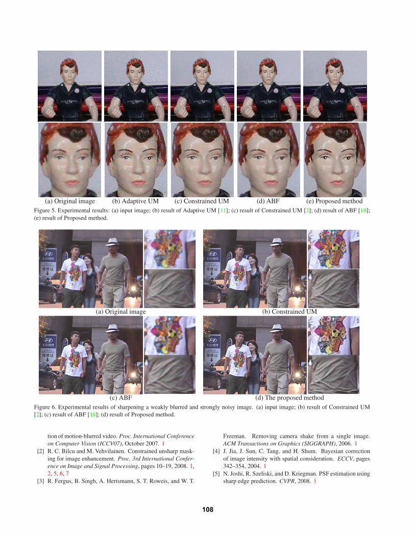
The next set of experimental results are shown in Fig.

6. The original image in (a) suffers from mild out-of-

focus blur and looks noisy because of bad illumination and

JPEG compression. Constrained UM restored image in (b)

looks much sharper, but the noise effects are also magni-

fied, which is probably because in the Constrained UM al-

gorithm unfiltered high-frequency components of the input

image are directly added to the output. ABF successfully re-

moved random noise and blocking artifacts caused by com-

pression, but again the sharpening strength is not strong. Al-

though it makes edges sharper without any overshoot, some

image details are smoothed. So visually the result in (c)

looks more blurry compared with (b) or (d). The proposed

method successfully removed both blur and noise artifacts,

making the restored structure more natural (see Fig. 6 (d)).

It also suppressed false color.

Additional results are given in Fig. 7, where again Con-

strained UM and ABF do not perform well in either noise

suppression or sharpening. On the other hand, this is a typ-

ical example of strong chrominance artifacts, which are ef-

fectively removed only by the proposed algorithm. (see Fig.

7 (b)-(d)).

4. Conclusion

In this paper, we developed a locally adaptive restoration

algorithm based on an extension of the steering kernel re-

gression technique. This algorithm is able to capture local

image structure and thus effectively combine denoising and

sharpening together. Experiments show that the proposed

approach can efficiently restore images distorted by weak

blur and strong noise. Compared with other state of the art

adaptive sharpening methods, it handles both denoising and

sharpening tasks simultaneously very well, and is capable

of removing chrominance artifacts. This algorithm is also

computationally cheap, since it is not iterative.

References

[1] L. Bar, B. Berkels, G. Sapiro, and M. Rumpf. A variational

framework for simultaneous motion estimation and restora-

3In general, Adaptive UM [11] produces similar sharpening effects as

Constrained UM [2], but with stronger noise artifacts. Its experimental

results for the remaining test images are not given due to space limit.

107

(a) Original image (b) Adaptive UM (c) Constrained UM (d) ABF (e) Proposed method

Figure 5. Experimental results: (a) input image; (b) result of Adaptive UM [11]; (c) result of Constrained UM [2]; (d) result of ABF [18];

(e) result of Proposed method.

(a) Original image (b) Constrained UM

(c) ABF (d) The proposed method

Figure 6. Experimental results of sharpening a weakly blurred and strongly noisy image. (a) input image; (b) result of Constrained UM

[2]; (c) result of ABF [18]; (d) result of Proposed method.

tion of motion-blurred video. Proc. International Conference

on Computer Vision (ICCV07), October 2007. 1

[2] R. C. Bilcu and M. Vehvilainen. Constrained unsharp mask-

ing for image enhancement. Proc. 3rd International Confer-

ence on Image and Signal Processing, pages 10–19, 2008. 1,

2, 5, 6, 7

[3] R. Fergus, B. Singh, A. Hertsmann, S. T. Roweis, and W. T.

Freeman. Removing camera shake from a single image.

ACM Transactions on Graphics (SIGGRAPH), 2006. 1

[4] J. Jia, J. Sun, C. Tang, and H. Shum. Bayesian correction

of image intensity with spatial consideration. ECCV, pages

342–354, 2004. 1

[5] N. Joshi, R. Szeliski, and D. Kriegman. PSF estimation using

sharp edge prediction. CVPR, 2008. 1

108

(a) Original image (b) Constrained UM (c) ABF (d) Proposed method

Figure 7. Experimental results: (a) input image; (b) result of Constrained UM [2]; (c) result of ABF [18]; (d) result of Proposed method.

[6] S. Kim and J. P. Allebach. Optimal unsharp mask for

image sharpening and noise removal. J. Electron. Imag.,

14(2):023007–1, 2005. 1

[7] A. Levin, R. Fergus, F. Durand, and W. T. Freeman. Image

and depth from a conventional camera with a coded aperture.

ACM Transactions on Graphics (SIGGRAPH), 2007. 1

[8] A. Levin, Y. Weiss, F. Durand, and W. T. Freeman. Un-

derstanding and evaluating blind deconvolution algorithms.

CVPR, 2009. 1

[9] M. Mahmoudi and G. Sapiro. Fast image and video denois-

ing via nonlocal means of similar neighborhoods. IEEE Sig-

nal Processing Letters, 12(12):839–842, Dec. 2005. 2

[10] S. H. Park, H. S. Kim, S. Lansel, M. Parmar, and B. Wandell.

A case for denoising before demosaicking. In Asilomar Con-

ference on Signals, Systems, and Computers, Pacific Grove,

CA, Nov. 2009. 4

[11] A. Polesel, G. Ramponi, and V. J. Mathews. Image enhance-

ment via adaptive unsharp masking. IEEE Transactions on

Image Processing, 9(3):505–510, March 2000. 1, 5, 6

[12] F. Russo. An image-enhancement system based on noise es-

timation. IEEE Trans. Instrumentation and Measurement,

56(4):1435–1442, August 2007. 1

[13] Q. Shan, J. Jia, and A. Agarwala. High-quality motion de-

blurring from a single image. ACM Transactions on Graph-

ics (SIGGRAPH), 2008. 1

[14] M. Sorel and P. Sroubek. Space-variant deblurring using one

blurred and one underexposed image. Proceedings of the

16th IEEE International Conference on Image Processing,

pages 157–160, 2009. 1

[15] H. Takeda, S. Farsiu, and P. Milanfar. Kernel regression for

image processing and reconstruction. IEEE Transactions on

Image Processing, 16(2):349–366, February 2007. 2, 3

[16] C. Tomasi and R. Manduchi. Bilateral filtering for gray and

color images. Proceeding of the 1998 IEEE International

Conference of Compute Vision, Bombay, India, pages 836–

846, January 1998. 2

[17] L. Yuan, J. Sun, L. Quan, and H. Shum. Image deblur-

ring with blurred/noisy image pairs. ACM Transactions on

Graphics (SIGGRAPH), 2007. 1

[18] B. Zhang and J. P. Allebach. Adaptive bilateral filter for

sharpness enhancement and noise removal. IEEE Transac-

tions on Image Processing, 17(5):664–678, May 2008. 1, 2,

5, 6, 7

[19] X. Zhu and P. Milanfar. Automatic parameter selection for

denoising algorithms using a no-reference measure of image

content. Accepted for IEEE Transactions on Image Process-

ing: 10.1109/TIP.2010.2052820. ISSN: 1057-7149. 4

[20] X. Zhu and P. Milanfar. A no-reference sharpness metric sen-

sitive to blur and noise. International Workshop on Quality

of Multimedia Experience (QoMEX), 2009. 4

109