Embed Size (px)
Citation preview

Journal of Business Studies, Vol. XXXIII, No. 1, June 2012
Responsiveness of Stock Prices to Changes in Macroeconomic Environment in Bangladesh
Sarkar Humayun Kabir* Abu Taleb**
Abdullah M. Noman*** Sadia Shermeen****
Abstract: This paper attempts to explore the long run relationship between stock prices and selected macroeconomic variables in Bangladesh by applying the time series analysis using monthly data from January 2001 to September 2010. We find a single cointegrating relationship among stock price and other selected macroeconomic variables. Analysis of the study also explores that stock prices and call money rate are the endogenous variables and all others variables are exogenous. Variance decomposition suggests that inflation rate is the leading exogenous variable influencing the stock prices. In addition, call money rate is found to be the leading endogenous variable. Above all, this study attempts to find the causes behind the 2010 stock market collapse in Bangladesh by establishing a relationship among the call money rate, stock prices, and bank lending to private sector in Bangladesh.
Keywords: Stock prices, Call money rate, Bangladesh, Vector Error Correction Model (VECM), Variance Decomposition, Impulse Response Functions, Persistence Profile functions
JEL Classification: E43, E44, E51, E62
*Sarkar Humayun Kabir, Assistant Professor of Finance, Faculty of Business Administration, American International University – Bangladesh (AIUB). Currently, He is pursuing PhD in Finance at INCEIF, Kuala Lumpur, Malaysia
**Abu Taleb, Professor in the Department of Banking and Insurance, Faculty of Business Studies, University of Dhaka, Dhaka 1000, Bangladesh.
***Abdullah M. Noman, Assistant Professor of Finance and Economics, Faculty of Business Administration, American International University – Bangladesh (AIUB). He is currently enrolled in the PhD in Financial Economics at University of New Orleans, Louisiana, USA.
****Sadia Shermeen, Associate Professor, Department of Marketing, University of Dhaka, Dhaka 1000, Bangladesh

202 Journal of Business Studies, Vol. XXXIII, No. 1, June 2012
1. Introduction
Pricing of stocks is one of the major areas of concern for the publicly listed firms. Not only for the firms, it is also one of the major interest areas even for the academicians, researchers and policy makers. A number of factors, both internal and external to the firms, influence stock price of firms. Internal factors at the micro level like profitability, capital structure, dividend policy, and above all good governance are the most significant determinants of stock price of a firm. On the other hand, inflation, money supply, foreign exchange rate, gross domestic product etc. are the prime macroeconomic fundamentals to influence the stock price at the firm level. Firms are responsible to control the micro factors in order to increase shareholders wealth by raising stock prices through their better performances. Better management of fundamentals at the firm level to increase stock price may not be successful unless it is supported by macroeconomic fundamentals. All the factors are not equally important to influence stock price in all economies. Same factors may more or less important in stock price determination depending on the state of economy.
There are different models and theories to explore the dynamic relationship between stock price and macroeconomic variables. Several studies have attempted to capture the effect of economic forces on stock returns in different countries. For example, using, the Arbitrage Pricing Theory (APT), developed by Ross (1976), Chen et al. (1986) used some macroeconomic variables to explain stock returns in the US stock markets. The authors’ findings showed industrial production, changes in risk premiums, and changes in the term structure to be positively related to the expected stock returns, while both the anticipated and unanticipated inflation rates were negatively related to the expected stock returns (Gan, Lee, Young, and Zhang, 2006).
The main objective of this study is to find out the dynamic nexus between stock prices and some key macroeconomic variables such as exchange rate, money supply (M2), three–month Treasury bill rate (as a proxy of short term interest rate), inflation rate, call money rate, and banking sector lending to private sector in Bangladesh. In addition, this study attempts to explore the possible causes of the recent stock market crash of December 2010 in Bangladesh.
This study employs Johansen cointegration approach, vector error correction model, long run structural modeling, variance decomposition, impulse response functions, and persistence profile functions in order to find out macroeconomic driving forces of stock price in Bangladesh. The analysis finds one statistically significant theoretical relationship among stock price, exchange rate, money supply, T-bill rate Inflation, call money rate, and bank lending to private sector of Bangladesh. Moreover, the study

Responsiveness of Stock Prices to Changes in Macroeconomic Environment in Bangladesh 203
suggests that inflation rate is the leading exogenous and T-bill rate is least exogenous variables to influence the stock price. In addition, this study finds a triangle nexus among stock price, call money rate and bank lending to private sector as an explanation for the 2010 stock market collapse in Bangladesh. The remaining part of the study is organized as follows: section two describes the motivation behind the study; section three summarizes literature review; sources of data and variables are presented in section four; section five describes econometric modeling of the study; estimation results are presented in section six; and finally, the study is concluded with policy recommendations in section seven.
2. Motivation of the Study
A number of studies have been conducted by the researchers to explore the relationship between stock price and major macroeconomic variables in Bangladesh. Most of these studies have used multivariate regression approach. A few studies have applied cointegration and vector error correction approach to find out theoretical relation between macro variables and stock price. Possibly, this would be the first of this kind of study employing eight steps approach of time series analysis to determine the leading macroeconomic factors to influence stock price in Bangladesh. Eight steps of time series analysis include unit root test, optimal lag structure, cointegration test, long run structural modeling, vector error correction model, variance decomposition, impulse response and persistence profile. Moreover, this study attempts to check the effects of call money rate and bank lending to private sector on stock price of Bangladesh. This would be an important issue for Bangladesh as commercial banks are major investors in stock markets. The outcome of this study would be valuable for the policymakers to set their future strategies to boost up the stock market in Bangladesh. In addition, market players and investors may use the outcome of this study to take sound and smart investment decisions in Bangladesh stock market.
3. Literature Review
Dynamic relation between stock price and macroeconomic variables is one of the concerning areas for the researchers and academicians. Some factors directly influence stock prices and some factors influence indirectly. Frequently cited macroeconomic variables are GDP growth, industrial production rate, short-term interest rate, inflation rate, interest rate spread, exchange rate, current account balance, unemployment rate, fiscal balance, etc. Studies done by Fama (1981, 1990), Fama and French (1989), Chen et al. (1986), Chen (1991), Thornton (1993), Kaneko and Lee (1995), Abdalla and Murinde (1997) are notable for the developed economies. On the contrary, for the developing economies, a few studies include Mookerjee and Yu (1997) and Maysami and Koh

204 Journal of Business Studies, Vol. XXXIII, No. 1, June 2012
(2000) for Singapore, Kwon and Shin (1999) for South Korea, and Habibullah and Baharumshah (1996) and Ibrahim (1999) for Malaysia.
Two theoretical models are mostly used in the modeling of the stock market as pointed out by Moolman and Du Toit (2003): the efficient market hypothesis and the present value model. Most of the empirical research on the efficient market hypothesis was done following the random walk model. Fama (1970) has proposed that the efficient market theory is based on the fair game model. In contrast to the random walk hypothesis, which dealt with the behavior of prices over time, the fair game model focus on the price in a specified period. Theoretically, the present value model states that discounted value of future dividends determines the security price. Therefore, any factor affecting the flow of future dividends and discount rates will systematically influence stock price. One of the well established literature on this issue is credited to Chen et al (1986) which showed that the influence of variables such as interest rates and inflation on the discount rate and of the industrial production growth on the expected cash flows or dividends. In empirical studies, these and other
variables are usually used to proxy the influence of dividends on stock prices. Jondeau and Nicolai (1993) have shown that only in the US dividends explain stock prices, whereas in other countries dividends have to be replaced by proxies. In the empirical literature, dividends are usually replaced by proxies such as industrial production, unemployment or the state of the business cycle (Harasty and Roulet, 2000). Gordon and Shapiro (1956) assuming a constant growth rate of dividend, showed that equilibrium prices of a security is determined by its dividends, growth rare, and the discount rate.
Islam and Watanapalachaikul (2003) showed a strong, significant long-run relationship between stock prices and macroeconomic factors (interest rate, bonds price foreign exchange rate, price-earnings ratio, market capitalization, and consumer price index) during 1992-2001 in Thailand. Fifield, Power and Sinclair (2002) used cross-sectional data for 13 emerging markets to test the influence of selected domestic variables and global variables in explaining the stock market. They used inflation, exchange rate, short-term interest rate, GDP, money supply and the trade balance as domestic variables and world return, world inflation, commodity prices, world industrial production, oil price and US interest rates as global variables. They observed that domestic GDP, inflation, money supply, interest rates, as well as world production and world inflation are able to explain fluctuations in equity returns in emerging markets. Fang (2002) argued that currency depreciation adversely affects stock returns and increases market volatility over the period of the Asian crises (1997-1999). The implication for investors is that they have to evaluate the stability of foreign exchange markets prior to investing in stock markets. Spyrou (2001) found that inflation and stock returns are negatively related up to 1995

Responsiveness of Stock Prices to Changes in Macroeconomic Environment in Bangladesh 205
after which the relationship became insignificant. He argued that the change in the relationship is due to the increased role of monetary fluctuations. Maysami and Koh (2000) examined such relationships in Singapore and found that inflation, money supply growth, changes in short- and long-term interest rate and variations in exchange rate formed a cointegrating relation with changes in Singapore’s stock market levels.
Using quarterly data and applying cointegration and error correction model, Jefferis and Okeahalam (2000) found a positive relation between stock market and GDP, exchange rate and foreign interest rates and a negative relation between the stock market and domestic interest rates. They used quarterly data for the period 1985 to 1995 and modeled the JSE overall index as a function of domestic and foreign GDP, the real exchange rate and long- term domestic and foreign real interest rates. Mukherjee and Naka (1995) applied Johansen’s (1998) Vector Error Correction Model (VECM) to analyze the relationship between the Japanese Stock Market and exchange rate, inflation, money supply, real economic activity, long-term government bond rate, and call money rate. They found cointegrating relationship between stock price and other macro variables.
Chen (1991) argued that stock market returns are a function of expected economic growth through its influence on dividends. He empirically showed that lagged economic growth, the default spread, the term spread, short-term interest rates and the dividend-price ratio are important determinants of future stock market returns in the US. In addition, expected excess market return is negatively related to recent economic growth and positively related to future growth. Kaul (1990) explicitly models the relationship between expected inflation and stock market returns. His findings are in line with Fama’s (1981) proxy hypothesis and showed that the relationship between stock returns and expected inflation in the US is significant and negative.
Kanakaraj et al. (2008) have examined the trend of stock prices and various macro economic variables between the time periods 1997-2007 in India and have found a strong relationship between the two. Muhammad and Rasheed (2002) examine the exchange rates and stock price relationships for Pakistan, India, Bangladesh and Sri Lanka using monthly data from 1994 to 2000. The empirical results show that there is a bi-directional long-run causality between these variables for only Bangladesh and Sri Lanka. No associations between exchange rates and stock prices are found for Pakistan and India. Using Engle Granger cointegration test and error correction model, Husain (2006) has examined the causal relationship between stock price and real sector variables of Pakistan economy to check the impact of financial liberalization using annual data from 1959-60 to 2004-05. His study indicated the presence of a long run relationship between the stock prices and real sector variables. It is to be noted that the issue of relation between stock price and macroeconomic variables remain unsolved due to heterogeneous findings from the above studies.

206 Journal of Business Studies, Vol. XXXIII, No. 1, June 2012
4. Sources of Data and Variables
All macroeconomic data of Bangladesh used in this study are secondary level data collected from Datastream. Total 118 monthly observations are used starting from January 2001 to September 2010. Total seven macro variables are considered in this study, which are explained as follows:
Table 1: Variables used in the study
Variable Explanation
LSP
LER
LMS2
LTBR3M
LINFR
LCMR
LBLPS
Logarithm of Stock Price (DSE)
Logarithm of Exchange Rate BDT/US$
Logarithm of Money Supply (M2)
Logarithm of 3-month T-bill Rate
Logarithm of Inflation Rate
Logarithm of Call Money Rate
Logarithm of Bank Lending to Private Sector

Responsiveness of Stock Prices to Changes in Macroeconomic Environment in Bangladesh 207
Graph 1: Plot of all variables in the study
The above graph of the variables show that stock price and call money rate are highly volatile over the period and they move more or less in the same fashion especially at the end of year 2010. Money supply and bank lending in the private sector are the lease volatile and they show upward trend over the period in concern.
Descriptive statistics of the variables are presented in the following table:

208 Journal of Business Studies, Vol. XXXIII, No. 1, June 2012
Table 2: Descriptive Statistics of the Variables
LSP LER LMS2 LMS2 LTBR3M LINFR LCMR
Mean 1.98 1.42 2.00 1.76 1.66 1.97 1.94
Median
Maximum
Minimum
Std. Dev.
Skewness
Kurtosis
Jarque-
Bera
1.96
2.16
1.89
0.07
0.55
2.33
8.20
1.43
1.45
1.38
0.02
-0.34
1.45
13.90
1.99
2.10
1.90
0.06
0.07
1.79
7.21
1.91
2.19
0.62
0.40
-1.56
4.32
56.35
1.82
2.30
0.38
0.53
-1.19
3.30
28.48
1.99
3.06
-0.30
0.52
-1.21
6.50
88.64
1.94
2.06
1.83
0.06
-0.00
1.82
6.75
Descriptive statistics shows that standard deviation of stock price, call money rate, and inflation rate are relatively higher and thus they are highly volatile over the concerned period, which is evidenced by the graphs.
5. Econometric Modeling
This study employs the Johansen multivariate cointegration approach to test cointegration of the macroeconomic variables. Then this study applies long run structural modeling (LRSM) to estimate theoretically meaningful long-run relations by imposing identifying restriction on the long-run relation. After finding out the theoretically long run relations, this study employs vector error correction model (VECM) to determine the speed of the short-run adjustment towards long term equilibrium by the size of the error correction coefficient. Furthermore, the impulse response and Error Variance Decomposition analyses are applied to examine the relative exogeneity/endogeneity of the selected macroeconomic variables. Finally, this study employs persistence profile (PF) test to find out the time horizon required for the conintegrating relation to get back to equilibrium when there is a system-wide shock.

Responsiveness of Stock Prices to Changes in Macroeconomic Environment in Bangladesh 209
The Augmented Dickey-Fuller (ADF) and Philips-Perron (PP) tests are used to check the stationarity of the variables. The lag length for the time series analysis is determined by choosing the lag length given by the minimum Akaike Information Criteria (AIC) and Schwarz Information Criteria (SBC).
Augmented Dickey-Fuller (ADF) (1979, 1981) test involves the estimation of the following general specification,
∆ = + + +∑ ∆ + (1)
The Phillips-Perron (PP) (1988) test suggests a non-parametric method of controlling for higher order autocorrelation in a time series and is based on the following equation:
∆ = + +∑ ∆ + (2)
In both ADF and PP equations, represents the difference operator, α, β, and δ are coefficients to be estimated. X is the variable whose stationarity should be checked and ε is the residual term. The critical values for the Phillips-Perron test are the same as those for the Dickey-Fuller test (DF), and depend on whether the DF regression contains an intercept term or a time trend.
After testing the stationarity of the time series, Johansen cointegration techniques is applied to check the cointegration of stock price (DSE index) with the considered macroeconomic variables of Bangladesh. Johansen (1988) and Johansen and Juselius (1990) suggested to consider the vector autoregressive (VAR) model of the following form:
∆ = +∑ ∆ + + (3)
Where, is a vector of non-stationary variables and C is a constant term. The matrix consists of the short run adjustment parameters and matrix contains long run equilibrium relationship information between the Y variables. The could be decomposed into the product of two × matrix α and β so that = ˊ, where β matrix contains number of conintegration and represents the speed of adjustment parameters. Johansen (1988) and Johansen and Juselius (1990) developed two statistic for identifying the number of cointegrating vectors, which are Trace statistic ( !"# ) and the maximum Eigen value

210 Journal of Business Studies, Vol. XXXIII, No. 1, June 2012
statistic ($!%). These two statistics can be expressed as follows:
!"# = − ∑, - ln (1 − +) (4)
and,
$!% = −/01 − + -1 (5)
Where, is the estimated value of the ith characteristics root obtained from the estimated parameter matrix and T is the number of usable observations. The $!% statistic tests the null hypothesis that there are at least r cointegrating vectors as against the alternative of (r + 1) cointegrating vectors.
Once we find cointegration among the considered variables, we estimate the Vector Error Correction Model (VECM). The VECM implies that changes in the dependent variable are a function of the level of disequilibrium in the cointegrating relationship – i.e. the departure from the long-run equilibrium – as well as changes in other explanatory variables. Considering the variables of this study, the VECM can be represented as follows:
∆ = +∑ ∆ + + + (6)
In the equation (6), is the parameter matrix, which contains LSP, LER, LMS2, LTBR3M, LINFR, LCMR, and LBLPS variables and the error correction terms.
After estimating VECM, we can apply variance decomposition, which breaks down the variance of the forecast error for each variable into proportions attributable to each variable of the model including its own. The variable which is explained mostly by its own is the leading variable. The graphical representation of variance decomposition is called impulse response. This approach is to determine how each endogenous variable responds over time to a shock in that variable and in every other endogenous variable. The impulse response function traces the response of the endogenous variables to such shocks.
6. Estimation Results
6.1 Unit Root Test
This study employs both ADF and PP tests to check the stationarity of the variables.
Summary of the unit root tests are presented in Table 3:

Responsiveness of Stock Prices to Changes in Macroeconomic Environment in Bangladesh 211
Table 3: Summary of Unit root Tests
Variables ADF PP
LSP
LER
LMS2
LTBR3M
LINFR
LCMR
LBLPS
DLSP
DLER
DLMS2
DLTBR3M
DLINFR
DLCMR
DLBLPS
1.28
(0.89)
1.71
(0.74)
2.15
(0.50)
2.24
(0.46)
2.15
(0.50)
4.44
(0.00)
4.79
(0.00)
8.90
(0.00)
12.26
(0.00)
4.77
(0.00)
6.48
(0.00)
4.05
(0.00)
13.26
(0.00)
10.68
(0.00)
1.92
(0.63)
1.52
(0.82)
3.87
(0.01)
1.56
(0.79)
1.37
(0.86)
4.56
(0.00)
4.92
(0.00)
9.03
(0.00)
12.51
(0.00)
32.22
(0.00)
5.73
(0.00)
4.05
(0.00)
13.29
(0.00)
15.52
(0.00)
P-values are in the parenthesis

212 Journal of Business Studies, Vol. XXXIII, No. 1, June 2012
Both ADF and PP tests assumes null hypothesis of non stationarity against the alternative hypothesis of stationarity. The above test results conclude that all variables are non-statioanry at the level form and stationary at the first difference form except LCMR and LBLPS, which are stationary at both level and first difference form.
6.2 Determination of the order of the VAR model
The following table 4 suggests the order of the VAR for testing cointegration:
Table 4: Lag order of the selection
Lag LogL LR FPE AIC SC HQ
0 132.2654 NA 0.005500 -2.365142 -2.340731 -2.355239
1
2
3
4
5
6
360.3413
362.1423
362.1425
362.9491
363.2286
363.2929
447.9329*
3.504646
0.000452
1.540500
0.528797
0.120430
9.19e-05
9.06e-05*
9.23e-05
9.26e-05
9.38e-05
9.54e-05
-6.456600
-6.471032*
-6.453018
-6.449533
-6.436551
-6.419691
-6.407779*
-6.397802
-6.355378
-6.327482
-6.290090
-6.248820
-6.436795
-6.441325*
-6.413408
-6.400021
-6.377136
-6.350374
*Indicates lag order selected by the criterion
Both AIC(Akaike Information Criterion) and HQ (Hannan-Quinn Information Criterion) suggest lag order of 2. On the contrary, SC (Schwarz Information Criterion) suggests lag order of 1 for the VAR model. Therefore, this study considers lag order of 2.
6.3 Test of Cointegration with lag order 2
Presence of correlation indicates that there exists a theoretical relationship among the variables and they are in equilibrium in the long run in spite of short run deviation from each other. Masih et al (2010) stated that a test of cointegration, therefore, also can be

Responsiveness of Stock Prices to Changes in Macroeconomic Environment in Bangladesh 213
considered as a test of the extent of the level of arbitrage activity in the long term. Cointegration implies that these variables are interdependent and highly integrated (as if they are constituents of one integrated market). Cointegration also implies that each variable contains information for the prediction of other variables. Moreover, the evidence of cointegration has implications for portfolio diversification by the investors. The possibility of abnormal gain through portfolio diversification is limited in the long run in a cointegrated market.
Table 5: Johansen Maximum Likelihood results for cointegration Cointegration LR Test Based on Maximal Eigenvalue
H0 H1Statistic 95% critical 90% critical
R = 0
R � = 1
R � = 2
R � = 3
R � = 4
R � = 5
R � = 6
R = 1
R = 2
R = 3
R = 4
R = 5
R = 6
R = 7
54.84
35.71
22.87
18.53
13.08
8.08
5.31
49.32
43.61
37.86
31.79
25.42
19.22
12.39
46.54
40.76
35.04
29.13
23.10
17.18
10.55
Cointegration LR Test Based on Trace Stochastic Matrix
R = 0 R = 1 158.45 147.27 141.82
R � = 1
R � = 2
R � = 3
R � = 4
R � = 5
R � = 6
R = 2
R = 3
R = 4
R = 5
R = 6
R = 7
103.61
67.89
45.02
26.48
13.39
5.31
115.85
87.17
63.00
42.34
25.77
12.39
110.60
82.88
59.16
39.34
23.08
10.55

214 Journal of Business Studies, Vol. XXXIII, No. 1, June 2012
Maximum eigenvalue statistic for H0: r = 0 against H1: r =1 is 54.84 � 49.32 (95% critical value), which implies rejection of H0 and acception of H1 conclude that there exists one cointegrating relationship among the variables. Similarly, trace statistic H0: r = 0 against H1: r =1 is 158.45 � 147.27 (95% critical value), which indicates the same as max eigenvalue result, means there exists one cointegrating relationship among the variables. The evidence of cointegrating relationship implies that there exists a common force (such as arbitrage activity) that brings stock price and other macro variables of Bangladesh to equilibrium in the long term.
6.4 Long Run Structural Modeling (LRSM)
Cointegration indicates long term relationship among the variables but does not indicate theoretically meaning full coefficients, which can be indicated by the “long run structural modeling (LRSM)” by imposing identifying and over-identifying restrictions on the cointegrating vector. In order to estimate theoretically meaningful long-run coefficients, we impose identifying restriction A1 = 1 on the LSP and the result is presented in the following table 6:
Table 6: Maximum Likelihood estimates subject Exactly Identifying Restriction
Variables Vector 1 (A1 = 1)
Note: T-Ratios are in the parenthesis
LSP
LER
LMS2
LTBR3M
LINFR
LCMR
LBLPS
1.00
(None)
-14.49
(0.19)
-44.14
(0.20)
-0.21
(0.20)
-0.07
(0.097)
1.27
(0.22)
72.65
(0.23)
Responsiveness of Stock Prices to Changes in Macroeconomic Environment in Bangladesh 215
Above LRSM result shows the long run theoretical coefficients of the variables under the cointegration relationship. Coefficients of LER, LMS2, LTBR3M, and LINFR with negative sign and positive coefficients of LCMR and LBLPS are expected according to theories. Though all coefficients are insignificant, we proceed with vector 1 for the remaining analysis of the study due to strong theoretical relationship among the variables.
6.5 Vector Error Correction Model (VECM)
Presence of cointegration, however, is unable to tell us the direction of Granger causality between the variables as to which variable is leading and which variable is lagging (i.e., which variable is exogenous and which variable is endogenous) (Masih, et al, 2010). Vector error correction model (VECM) is applied to determine the endogeneity/exogeneity of the variables. The estimation of VECM is presented in the following table 7:
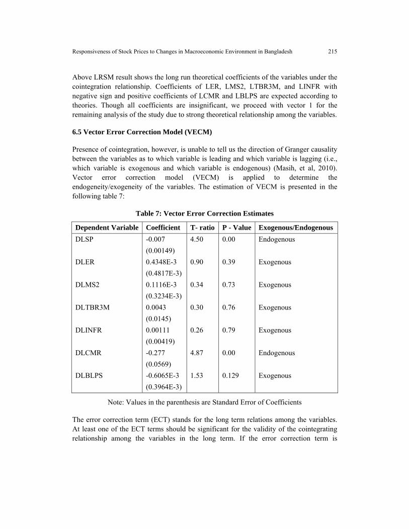
Table 7: Vector Error Correction Estimates
Dependent Variable Coefficient T- ratio P - Value Exogenous/Endogenous
DLSP
DLER
DLMS2
DLTBR3M
DLINFR
DLCMR
DLBLPS
-0.007
(0.00149)
0.4348E-3
(0.4817E-3)
0.1116E-3
(0.3234E-3)
0.0043
(0.0145)
0.00111
(0.00419)
-0.277
(0.0569)
-0.6065E-3
(0.3964E-3)
4.50
0.90
0.34
0.30
0.26
4.87
1.53
0.00
0.39
0.73
0.76
0.79
0.00
0.129
Endogenous
Exogenous
Exogenous
Exogenous
Exogenous
Endogenous
Exogenous
Note: Values in the parenthesis are Standard Error of Coefficients
The error correction term (ECT) stands for the long term relations among the variables. At least one of the ECT terms should be significant for the validity of the cointegrating relationship among the variables in the long term. If the error correction term is

216 Journal of Business Studies, Vol. XXXIII, No. 1, June 2012
insignificant, the corresponding dependent variable is ‘exogenous’. On the contrary, if the error correction term is significant, the corresponding dependent variable is ‘endogenous’. The size of the coefficient of the ECT indicates the speed of short term adjustment to bring about long-term equilibrium and it represents the proportion by which the disequilibrium in the dependent variable is being corrected in each short period. The size of the coefficient also indicates the intensity of arbitrage activity to bring about equilibrium. Finally, the VECM allows us to distinguish between the ‘short-term’ and ‘long-term’ Granger-causality.
VECM of this study suggests that stock price (LSP) is dependent (endogenous) variable in the cointegration relation. The error correction coefficient of DLSP is -0.007 with P-value = 0.00 � 0.05, which is statistically significant and suggesting that DLSP is “Endogenous” variable, i.e. it depends on the deviations of other variables. The coefficient 0.007 of the error correction term indicates the speed of short term adjustment to bring about long term equilibrium. Here disequilibrium in the LSP seems to be corrected by 0.7% in each short period. It also indicates arbitrage activity in the stock market seems to be corrected by 0.7% in each short (quarter) to bring the market back to equilibrium. VECM also suggests that call money rate (LCMR) is another “Endogenous” variable. Apart from LSP and LCMR, all other variables in the cointegrating relationship are exogenous variables as suggested by the VECM.
6.6 Variance Decomposition
Vector error correction model (VECM) determines the endogeneity/exogeneity of the variables but does not tell us anything about relative exogeneity/endogeneity of the variables, which variance decomposition does. Variance decomposition is a process of decomposing the variance of the forecast error of a particular variable into proportions attributable to shocks (or innovations) in each variable in the system including its own. The relative exogeneity/endogeneity of a variable can be determined by the proportion of the variance explained by its own past shocks. The variable which is explained mostly by its own shocks is deemed to be the most exogenous/endogenous variable. This study employs generalized variance decomposition technique in order to determine relative endogeneity/exogeneity of the variables in the cointegrating relationship. The result of the variance decomposition is presented in the following table 8:

Responsiveness of Stock Prices to Changes in Macroeconomic Environment in Bangladesh 217
Table 8: Generalized Variance Decomposition Analysis Percentage of Forecast Variance Explained by Innovations in:
LSP LER LMS2 LINFR LTBR3M LCMR LBLPSMonth 1 3 5 10 Month 1 3 5 10 Month 1 3 5 10 Month 1 3 5 10 Month 1 3 5 10 Month 1 3 5 10 Month 1 3 5 10
LSP LER LMS2
LINFR
LTBR3M LCMR
LBLPS
92.47 78.34 61.06 42.42 0.00 0.22 0.18 0.13 0.00 3.47 2.93 2.43 0.00 0.13 0.17 0.10 0.04 0.26 0.35 0.31 0.00 2.21 1.78 1.45 0.00 0.72 0.59 0.46
0.85 1.38 1.21 1.40 93.60 85.85 82.58 79.21 0.05 0.44 0.82 1.01 0.82 1.16 0.80 0.57 0.13 0.04 0.31 0.46 0.00 3.48 5.59 7.49 0.00 1.09 1.11 1.82
3.56 2.92 7.04 10.90 0.00 0.07 0.40 0.63 91.78 84.89 83.80 82.42 0.00 0.50 0.49 1.52 0.99 0.72 0.75 0.40 0.00 1.30 1.55 6.26 0.00 0.99 0.98 1.81
0.06 0.47 0.29 0.42 0.00 0.15 0.35 1.20 1.31 2.27 2.76 2.80 97.12 96.80 96.56 95.90 2.87 8.55 13.09 19.36 0.00 3.62 4.49 4.34 0.00 1.19 2.24 3.31
0.00 0.35 0.32 0.48 0.00 0.08 0.26 0.35 0.00 0.97 0.78 0.47 0.00 0.73 1.08 0.73 93.41 77.98 69.17 64.58 0.00 6.45 5.53 4.35 0.00 0.72 0.59 0.46
2.94 16.06 28.56 42.46 5.61 12.71 15.50 17.90 0.12 0.12 0.08 0.34 2.00 0.42 0.55 0.26 2.52 12.30 15.99 13.95 98.51 81.48 78.48 69.70 0.00 2.04 1.75 5.32
0.12 0.47 1.52 1.92 0.79 0.91 0.74 0.59 6.75 7.83 8.82 10.54 0.07 0.24 0.35 0.92 0.02 0.13 0.32 0.93 1.49 1.46 2.58 6.41 100.00 93.10 92.51 86.76
We got two endogenous variables namely, stock price and call money rate from the VECM analysis. Above result of variance decomposition analysis shows that 42.42 percent of the forecast error variance of stock price is explained by its own shock in the tenth month. On the contrary, in the case of call money rate, 69.70 percent of the forecast error variance is explained by its own shock during the same time period, which indicates that call money rate is the leading endogenous variable.

218 Journal of Business Studies, Vol. XXXIII, No. 1, June 2012
In case of exogenous variables, VECM result shows that inflation rate is the most (leading) exogenous variable as 95.90 percent of the forecast error variance is explained by its own shock in the tenth month. In the exogenous list, three month T-bill rate is the least exogenous variable as only 64.58 percent of the forecast error variance is explained by its own shock during the same time period, which is the smallest among all exogenous variables. Surprisingly, call money rate is contributing significantly in the forecast of error variance of both stock price and exchange rate. Proportional contribution of call money rate to the forecast error variance of stock price and exchange rate in the tenth month is 42.46 percent and 17.90 percent respectively. Among other exogenous variables, bank lending to private sector is contributing 10.54 percent to the forecast error variance of money supply and proportional contribution of inflation rate is 19.36 percent to the forecast error variance of three month T-bill rate in the tenth period.
This result shows that call money rate is one of the most significant variables to influence the stock price and exchange rate in Bangladesh. This finding is evidenced by the simultaneous movement of stock price and call money rate in the same direction, especially, in December 2010 immediately after which, the stock market crash started in Bangladesh. It is suspected that sudden withdrawal of banks’ investment from the stock market at the financial year end in order to compute annual profit added fuel to the stock market turmoil in Bangladesh. Moreover, banks were facing liquidity shortage, which contributed to the hike in call money rate as many new generation bank’s liquid fund was blocked in the stock market as stock price was declining eventually.
6.7 Impulse Response Function (IRF)
Impulse response function (IRF) is the graphical representation of variance
decomposition. IRFs essentially map out the dynamic response path of a variable owing to shock to another variable. IRFs of this study are presented in the following graph:
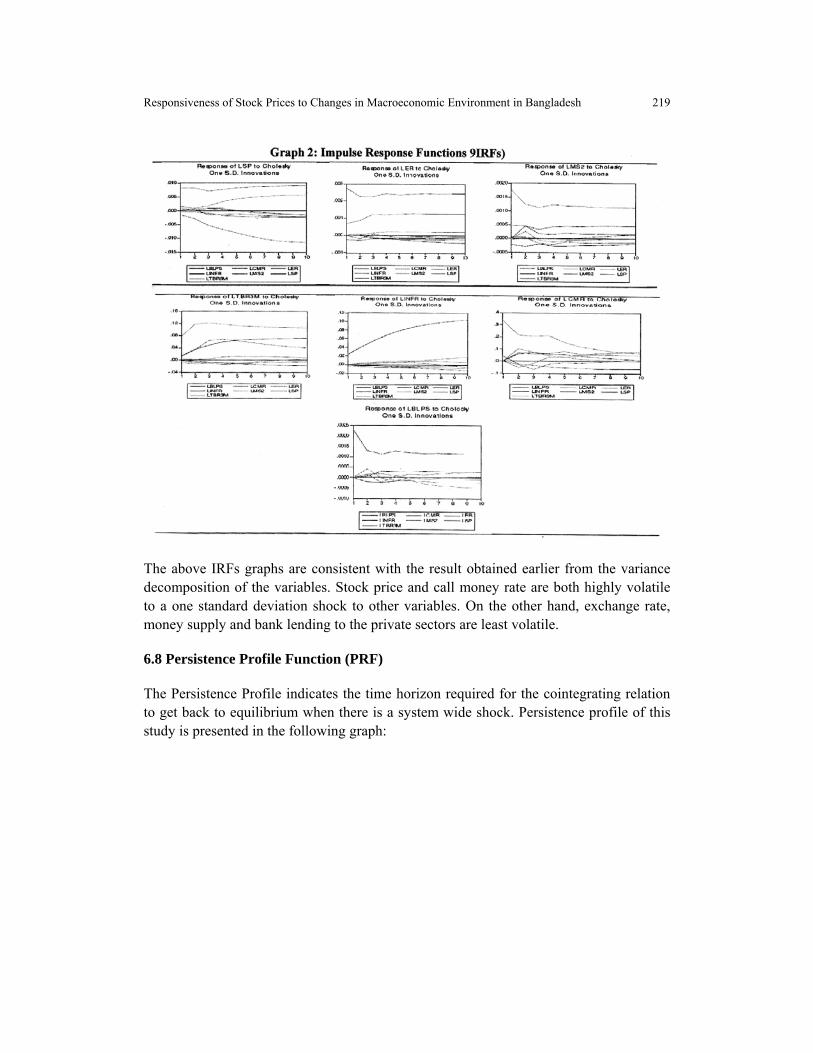
Responsiveness of Stock Prices to Changes in Macroeconomic Environment in Bangladesh 219
The above IRFs graphs are consistent with the result obtained earlier from the variance decomposition of the variables. Stock price and call money rate are both highly volatile to a one standard deviation shock to other variables. On the other hand, exchange rate, money supply and bank lending to the private sectors are least volatile.
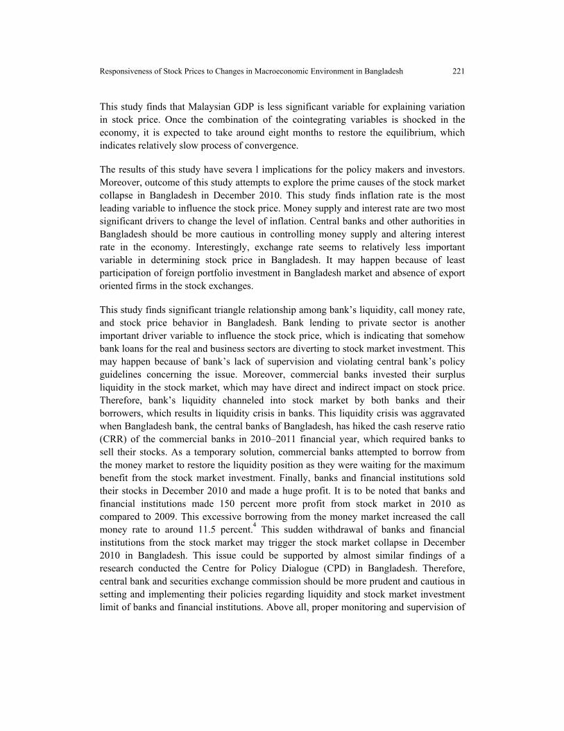
6.8 Persistence Profile Function (PRF)
The Persistence Profile indicates the time horizon required for the cointegrating relation to get back to equilibrium when there is a system wide shock. Persistence profile of this study is presented in the following graph:

220 Journal of Business Studies, Vol. XXXIII, No. 1, June 2012
The above PRF graph indicates that it may take about eight months to restore the equilibrium once the whole cointegrating relationship is shocked in the economy, which is not very quick speed of convergence.
7. Conclusion and Policy Recommendation
This study attempts to explore the dynamic relationship between stock price and selected macroeconomic variables in Bangladesh. Applying Cointegration, long run structural modeling, vector error correction model, variance decomposition, impulse response, and persistence profile, this study concludes with the following observations.
There is a statistically significant long run relationship among stock price, exchange rate, money supply, T-bill rate Inflation, call money rate, and bank lending to private sector of Bangladesh. Therefore, a linear combination of these variables tends toward equilibrium/stationarity.
Stock price and call money rate are found to be dependent (endogenous) variable and BDT/US$ exchange rate, money supply, T-bill rate, inflation, and bank lending to private sector are independent (exogenous) variables. This study attempts to explore the theoretical relationship of stock price with other macro variables even though we found two statistically significant endogenous variables. Surprisingly, between the two endogenous variables, according to variance decomposition, call money rate is more endogenous than stock price. This result implies a significant inter linkage of bank liquidity, stock market investment strategy, and stock price in Bangladesh. Among all exogenous variables, inflation rate is the most exogenous and T-bill rate is the least exogenous variable, which implies that stock price moves mostly in response to any movement in the inflation rate. Change in T-bill rate has the least impact on stock price behavior in Bangladesh.
Responsiveness of Stock Prices to Changes in Macroeconomic Environment in Bangladesh 221
This study finds that Malaysian GDP is less significant variable for explaining variation in stock price. Once the combination of the cointegrating variables is shocked in the economy, it is expected to take around eight months to restore the equilibrium, which indicates relatively slow process of convergence.
The results of this study have severa l implications for the policy makers and investors. Moreover, outcome of this study attempts to explore the prime causes of the stock market collapse in Bangladesh in December 2010. This study finds inflation rate is the most leading variable to influence the stock price. Money supply and interest rate are two most significant drivers to change the level of inflation. Central banks and other authorities in Bangladesh should be more cautious in controlling money supply and altering interest rate in the economy. Interestingly, exchange rate seems to relatively less important variable in determining stock price in Bangladesh. It may happen because of least participation of foreign portfolio investment in Bangladesh market and absence of export oriented firms in the stock exchanges.
This study finds significant triangle relationship among bank’s liquidity, call money rate, and stock price behavior in Bangladesh. Bank lending to private sector is another important driver variable to influence the stock price, which is indicating that somehow bank loans for the real and business sectors are diverting to stock market investment. This may happen because of bank’s lack of supervision and violating central bank’s policy guidelines concerning the issue. Moreover, commercial banks invested their surplus liquidity in the stock market, which may have direct and indirect impact on stock price. Therefore, bank’s liquidity channeled into stock market by both banks and their borrowers, which results in liquidity crisis in banks. This liquidity crisis was aggravated when Bangladesh bank, the central banks of Bangladesh, has hiked the cash reserve ratio (CRR) of the commercial banks in 2010–2011 financial year, which required banks to sell their stocks. As a temporary solution, commercial banks attempted to borrow from the money market to restore the liquidity position as they were waiting for the maximum benefit from the stock market investment. Finally, banks and financial institutions sold their stocks in December 2010 and made a huge profit. It is to be noted that banks and financial institutions made 150 percent more profit from stock market in 2010 as compared to 2009. This excessive borrowing from the money market increased the call money rate to around 11.5 percent.
4 This sudden withdrawal of banks and financial
institutions from the stock market may trigger the stock market collapse in December 2010 in Bangladesh. This issue could be supported by almost similar findings of a research conducted the Centre for Policy Dialogue (CPD) in Bangladesh. Therefore, central bank and securities exchange commission should be more prudent and cautious in setting and implementing their policies regarding liquidity and stock market investment limit of banks and financial institutions. Above all, proper monitoring and supervision of

222 Journal of Business Studies, Vol. XXXIII, No. 1, June 2012
these two organizations over bank lending to private sector and irregular behavior of stock prices are crucial to avoid possible stock market slump in Bangladesh.
--------------------------------------------
4 Article published in the “Daily Prothom Alo” on June 5, 2011 regarding relation between stock market and bank’s liquidity.
References
Abdalla, I. S. A., and V. Murinde, (1997). “Exchange Rate And Stock Price Interactions In Emerging Financial Markets: Evidence on India, Korea, Pakistan, and Philippines”, Applied Financial Economics, 7, 25-35.
Chen N. F., R. Roll and S. A. Ross (1986). “Economic Forces and the Stock Market”, Journal of Business, Vol. 59, No. 3, pp. 383-403.
Chen, N. F. (1991). “Financial Investment Opportunities and the Macroeconomy”. Journal of Finance, Vol. XLVI, No. 2, 529-544.
Dickey, D. A. and W. A. Fuller (1979). “Distribution of the Estimators for Autoregressive Time Series with a Unit Root,” Journal of the American Statistical Association, Vol. 74, pp. 427-431.
________________________ (1981). “Likelihood Ratio Statistics for Autoregressive Time Series with a Unit Root”, Econometrica, Vol. 49, PP. 1057 – 1072.
Fama, E. F. (1981). “Stock returns, real Activity, inflation and money”, The American Economic Review, 71(4), 45-565.
Fama, E. F. (1990). “Stock returns, expected returns and real activity”, Journal of Finance, 45(4), 1089-1108.
Fama, E. F. (1970). “Efficient Capital Markets: A review of theory and empirical work.” Journal of Finance, 25(2): 383 – 417.
Fama E. F. and French L. (1989). “Business conditions and expected prices on stocks and Bonds”, Journal of Financial Economics, 25, 23-49.
Fang, W. (2002). “The effects of currency depreciation on stock returns: Evidence from five East Asian economies”, Applied Economics Letters, Vol. 9 (3):195-199, 2002.

Responsiveness of Stock Prices to Changes in Macroeconomic Environment in Bangladesh 223
Fifield, S. G. M., Power, D. M. and Sinclair, C. D. (2002), “Macroeconomic factors and share returns: an analysis using emerging market data”, International Journal of Finance and Economics, Vol. 7: 51-62.
Gan, Lee, Young, and Zhang (2006). “Macroeconomic Variables and Stock Market Interactions: New Zealand Evidence, Investment Management and Financial Innovations, Volume 3, Issue 4, pp: 89 – 101.
Gordon, M. J. and Shapiro, E. (1956). Capital Equipment Analysis: The required rate of profit, Management Science, October 53-61.
Habibullah, M. S. and Baharumshah, A.Z. (1996). “Money, output, and stock prices in Malaysia: An application of the co-integration tests”, International Economic Journal, 10(2), 121-130.
Harasty, H. and Roulet, J. (2000). Modeling Stock Market Returns, Journal of Portfolio Management, Vol. 26 (2): 33.
Husain, F. (2006). “Stock Prices, Real Sector and the Causal Analysis: The Case of Pakistan”, Journal of Management and Social Sciences. 2, 179-185
Ibrahim, M. H. (1999). “Macroeconomic variables and stock prices in Malaysia: An empirical analysis”, Asian Economic Journal, 13(2), 219-231.
Islam, S. M. N. & Watanapalachaikul, S. (2003). “Time series financial econometrics of the Thai stock market: a multivariate error correction and valuation model”, available at http://blake.montclair.edu/~cibconf/conference/DATA/Theme2/Australia2.pdf
Jefferis, K. R. and Okeahalam, C. C. (2000). “The impact of economic fundamentals on stock markets in southern Africa”. Development Southern Africa, 17(1):23-51.
Johansen, S. (1988). “Statistical Analysis of Cointegration Vectors”, Journal of Economic Dynamics and Control, Vol. 12, pp. 231-254.
Johansen, S., and Juselius, K., (1990). “Maximum Likelihood Estimation and Inference on Cointegration with Applications to the Demand for Money,” Oxford Bulletin of Economics and Statistics, 52, 169-210.
Jondeau, E. and Nicolai, J. P. (1993). Modelisation du Prix des Actifs Financiers, Document d’Etude, Groupe Caisse des Depots, Service des Etudes Economiques et Financieres, 16/F: 1 - 85.
Kanakaraj, A., Singh, B. K. and Alex, D. (2008). “Stock Prices, Micro Reasons and Macro Economy in India: What do data say between 1997-2007”, Fox Working Paper 3. 1-17.
Kaneko T, Lee BS (1995). “Relative importance of the economic factors in the U.S. and Japanese stock markets”, J. Jpn. Int. Econ. 9(3): 209-307.
224 Journal of Business Studies, Vol. XXXIII, No. 1, June 2012
Kaul, G., (1990). “Monetary Regimes and the relation between stock returns and inflationary expectations”, Journal of Financial and quantitative analysis, Vol. 15: 307-321, 1990.
Kwon, C. S. and Shin, T. S. (1999). “Co-integration and causality between macroeconomic variables and stock market returns” Global Finance Journal, 10(1), 71-81.
Masih, M., Sahlawi, M. A. A. and Mello, L. D. (2010). “WHAT DRIVES CARBON-DIOXIDE EMISSIONS: INCOME OR ELECTRICITY GENERATION? EVIDENCE FROM SAUDI ARABIA”, The Journal of Energy and Development, Vol. 33, No. 2, pp. 201- 213
Maysami, R. C. & Koh, T. S. (2000). “A vector error correction model of the Singapore stock market”, International Review of Economics and Finance 9: 79-96.
Mokerjee, Rajen and Qiao Yu (1997). “Macroeconomic Variables and Stock Prices in a Small Open Economy: The Case of Singapore”, Pacific-Basin Finance Journal, 5, 377-388.
Moolman, E. and Du Toit, C. (2003). An Econometric Model of the South African Stock Market, Eight Annual Conference on Econometric Modeling for Africa, 1-4 July 2003.
Muhammad, Naeem and Rasheed, Abdul, (2002). “Stock Prices and Exchange Rates: Are They Related? Evidence from South Asian Countries”, The Pakistan Development Review, 41(4), 535-550.
Mukherjee, T. K. & Naka, A. (1995). “Dynamic relations between macroeconomic variables and the Japanese stock market: an application of a vector error correction model”, The Journal of Financial Research 18(2): 223-237.
Phillips, P. C. and Perron, P. (1988). “Testing for a Unit Root in Time Series Regressions”, Biometrika, Vol. 32, pp.301 – 318.
Ross, S. A. (1976). “The Arbitrage Theory of Capital Asset Pricing”, Journal of Economic Theory, Vol. 13, No. 3, pp. 341-360.
Spyrou, I. S. (2001). “Stock returns and inflation: evidence from an emerging market”, Applied Economics Letters, Vol. 8:447-450.
Thornton J. (1993). “Money, output and stock prices in the UK”, Applied Financial Economics, 3(4), 335-338.