Response variability of stochastic frame structures …users.ntua.gr/vpapado/Publications/Publication8.pdfResponse variability of stochastic frame structures using evolutionary ﬁeld

Comput. Methods Appl. Mech. Engrg. 195 (2006) 1050–1074

www.elsevier.com/locate/cma

Response variability of stochastic frame structuresusing evolutionary field theory

Vissarion Papadopoulos a,*, George Deodatis b

a Institute of Structural Analysis and Seismic Research, National Technical University of Athens, 9 Iroon Polytechneiou,

Zografou Campus, Athens 15780, Greeceb Department of Civil Engineering and Engineering Mechanics, Columbia University, New York, NY 10027, USA

Received 8 November 2004; received in revised form 31 March 2005; accepted 8 April 2005

Abstract

The integral form for the variance of the response of stochastic statically indeterminate structural systems involvingthe so-called variability response function (VRF) and the spectral density function of the stochastic field modelling theuncertain system properties is established for the first time in this paper using evolutionary spectra theory. The VRF is afunction depending on deterministic parameters related to the geometry, boundary conditions, (mean) material prop-erties and loading of the structural system. No approximations are involved in the derivation of the integral form. How-ever, a conjecture has to be made that is validated using Monte Carlo simulations. The uncertain system propertyconsidered is the inverse of the elastic modulus (flexibility). Closed-form expressions can be derived in principle forthe VRF of any statically determinate or indeterminate frame system using a flexibility-based formulation. Alterna-tively, a fast Monte Carlo simulation approach is provided to numerically evaluate the VRF. It is shown in closed-formand numerically that the VRF for statically indeterminate structures is a function of the standard deviation rff of thestochastic field modeling the inverse of the elastic modulus. Although the VRF depends on rff, it appears to be inde-pendent of the functional form of the spectral density function of the stochastic field modeling the uncertain systemproperties. For statically determinate structures, the VRF is independent of rff. The integral form can be used to com-pute the variance of the system response as well as its upper bound with minimal computational effort. It also providesan excellent insight into the mechanisms controlling the response variability. The upper bounds for the response var-iance are spectral- and probability-distribution-free requiring knowledge of only the variance of the inverse of the elasticmodulus. The proposed bounds are realizable in the sense that it is possible to determine the probabilistic characteristicsof the stochastic field that produces them. Several numerical examples are provided demonstrating the capabilities ofthe methodology.� 2005 Elsevier B.V. All rights reserved.

0045-7825/$ - see front matter � 2005 Elsevier B.V. All rights reserved.doi:10.1016/j.cma.2005.04.003

* Corresponding author.E-mail addresses: [email protected] (V. Papadopoulos), [email protected] (G. Deodatis).

mailto:[email protected]

mailto:[email protected]

V. Papadopoulos, G. Deodatis / Comput. Methods Appl. Mech. Engrg. 195 (2006) 1050–1074 1051

Keywords: Variability response function; Stochastic finite element analysis; Non-homogeneous stochastic fields; Upper bounds; MonteCarlo simulation

1. Introduction

The analysis of stochastic systems with material/geometric properties modelled by random fields hasbeen the subject of extensive research in the past two decades. The majority of the work has focused ondeveloping stochastic finite element methodologies (SFEM) for the numerical solution of the stochastic dif-ferential equations involved in the problem. By far, the most widely used SFEM approaches are approxi-mate expansion/perturbation based methods. Although such methods have proven to be highly accurateand computationally efficient for a variety of problems, there is still a wide range of problems in stochasticmechanics involving combinations of strong non-linearities, large variations of system properties and non-Gaussian system properties that can be solved with reasonable accuracy only through a computationallyexpensive Monte Carlo simulation approach.

Whether an expansion/perturbation based approach or a Monte Carlo simulation methodology is usedto estimate the response variability of a stochastic system, it is necessary to know the probability distribu-tion function (PDF) and the spectral/correlation characteristics of the stochastic system properties. In mostpractical engineering applications, there is a lack of experimental data that would enable a quantification ofsuch probabilistic characteristics of the stochastic system properties. Taking into account that manyresearchers have clearly demonstrated that both the correlation structure and the PDF of the material/geo-metric properties can have a significant (and in certain cases dramatic) effect on the stochastic response, aSFEM or Monte Carlo analysis will not provide particularly useful results for real-life applications whenthe probabilistic characteristics of the system properties are arbitrarily assumed.

A common approach to address the aforementioned problem is to perform a sensitivity analysis withrespect to the various parameters controlling the probabilistic characteristics of the stochastic system prop-erties. Although such an approach has obvious advantages, it also has certain drawbacks. First, the com-putational effort increases drastically as the number and range of the various parameters examined expand.Then, there is no real insight on the effect of the various parameters on the response variability of the sys-tem. And finally, it is practically impossible to determine upper bounds on the response variability as thenumber of combinations of the various parameters is essentially infinite.

To address all three of the above drawbacks, the concept of variability response function (VRF) wasintroduced in the late 1980s. The basic idea associated with the VRF is to express the variance of the re-sponse (i.e. displacement) in the following integral form:

Var½u� ¼Z 1

�1VRFðjÞSff ðjÞdj; ð0aÞ

where the VRF is a function depending on deterministic parameters related to the geometry, boundary con-ditions, (mean) material properties and loading of the structural system, Sff(j) is the spectral density functionof the stochastic field modeling the uncertain material/geometric properties, and j is the wave number.

It is straightforward to see how the concept of the VRF in conjunction with the integral form in Eq. (0a)addresses all three drawbacks mentioned above. Once the VRF is determined, the variance of the responsecan be estimated very easily through a simple integration given any form of the spectral density functionSff(j) (the VRF is usually a smooth function of j). Eq. (0a) also provides an excellent insight of the effectof the form of the spectral density function of the stochastic field modeling the uncertain material/geometricproperties on the response variability. Finally, a spectral- and probability-distribution-free upper bound forthe response variance can be computed in a straightforward way as:

1052 V. Papadopoulos, G. Deodatis / Comput. Methods Appl. Mech. Engrg. 195 (2006) 1050–1074

Var½u� 6 VRFðjmaxÞr2ff ð0bÞ

with jmax being the wave number where the VRF attains its maximum value and r2ff being the variance of

the stochastic field modeling the material/geometric properties.Early work determined the VRF for a wide range of problems (beams, frames, plane stress/strain, plate

bending, random eigenvalue problem) using some kind of first-order approximation (usually of the re-sponse displacement). An immediate consequence was that even the existence of the integral form in Eq.(0a) depended on this approximation. The uncertain system property in this early work was always the elas-tic modulus. A more detailed description of the early developments in this field, including a list of relevantreferences until the present, can be found in [3] where it was attempted for the first time to establish theintegral form in Eq. (0a) without having to go through a first-order approximation. The key was to considerthe inverse of the elastic modulus as the uncertain system property. For the case of statically determinatebeam structures, the existence of the integral form in Eq. (0a) was easily established in a rigorous mathe-matical way and closed-form expressions were provided for the VRF. For statically indeterminate beamstructures, however, a conjecture had to be made about the existence of an integral form like the one inEq. (0a) and the VRF was subsequently estimated numerically. The validity of this conjecture was demon-strated numerically through a brute-force optimization scheme involving the computation of upper boundsof the response variance. Consequently, because the conjecture was based mostly on insight and because ofthe process followed to validate it, Papadopoulos et al. [3] used Eq. (0a) in an ad hoc way to determine onlyupper bounds of the response variance (and not the response variance itself).

The present paper complements and extends the work done in [3] in the following ways. First, the inte-gral form in Eq. (0a) for statically indeterminate structures is formulated in a different way using the con-cept of non-homogeneous evolutionary fields developed by Priestley [4]. Although a rigorous mathematicalproof of the existence of the integral form in Eq. (0a) is still elusive for statically indeterminate structures, adifferent conjecture is made now regarding the existence of a non-homogeneous evolutionary stochasticfield involving the uncertain elastic properties. Furthermore, this alternative conjecture is now validatednumerically by computing the response variance through Eq. (0a) and comparing it with Monte Carlo sim-ulation predictions. There is still no first-order approximation involved as the inverse of the elastic modulusis again considered as the uncertain system property. Closed-form expressions can be established in prin-ciple for the variability response function of any statically determinate or indeterminate frame system usinga flexibility-based formulation. In contrast to the conclusions in [3], it is shown here that the VRF for stat-ically indeterminate structures is a function of the standard deviation rff of the stochastic field modeling theinverse of the elastic modulus. The dependence of VRF on rff is negligible in some cases and this is the rea-son that it was not detected numerically in [3]. In the present paper, the dependence of the VRF on rff forstatically indeterminate structures is established in closed-form expressions. It is pointed out that althoughthe VRF depends on rff, it appears to be independent of the functional form of the spectral density functionSff(j). For statically determinate structures, the VRF is independent of rff as well.

The integral form in Eq. (0a) is therefore established in this paper using a different formulation involvingan alternative conjecture compared to [3]. In addition, the validation of the conjecture is done in a muchstricter way in this paper: by comparing the response variance predictions of Eq. (0a) with Monte Carlosimulations (compared to a brute-force optimization validation in [3] involving the upper bound of the re-sponse variance). Consequently, Eq. (0a) is used in this paper with confidence to compute the variance ofthe response through a simple integration, as well as to estimate its upper bound (compare to [3] where itwas used only to estimate upper bounds).

The upper bounds established in this study for the response variability are spectral- and probability-dis-tribution-free requiring knowledge of only the variance of the inverse of the elastic modulus. It should bementioned that the variance of the inverse of the elastic modulus can be obtained as easily as the variance ofthe elastic modulus using the same experimental data. The proposed bounds are realizable in the sense that


it is possible to determine the probabilistic characteristics (spectral density function and marginal probabil-ity distribution function) of the stochastic field (modeling the inverse of the elastic modulus) that producesthem. Furthermore, it is possible to fully determine also the corresponding stochastic field modeling theelastic modulus that produces these bounds.

Finally, it should be mentioned that the approach used in this paper to model the beam flexibility insteadof its rigidity has already been followed in a small number of earlier studies (e.g. [1]). In these studies, exactexpressions for the response variance were established for simple statically determinate beams under staticloading (but not in the form of Eq. (0a) involving the variability response function).

2. Statically determinate beams

Consider the statically determinate beam of length L shown in Fig. 1, carrying a deterministic uniformlydistributed load Q0. The inverse of the elastic modulus of the beam is assumed to vary randomly along itslength according to the following expression:

1

EðxÞ ¼ F 0ð1þ f ðxÞÞ; ð1Þ

where E is the elastic modulus, F0 is the mean value of the inverse of E, and f(x) is a zero-mean homoge-neous stochastic field modeling the variation of 1/E around its mean value F0.

The response displacement of the beam u(x) is given by:

uðxÞ ¼ F 0Q0

2I

Z x

0

ðx� nÞðL� nÞ2ð1þ f ðnÞÞdn ¼Z x

0

gðx; nÞð1þ f ðnÞÞdn; ð2Þ

where I is the moment of inertia and:

gðx; nÞ ¼ F 0Q0

2Iðx� nÞðL� nÞ2. ð3Þ

As described in detail in [3], the variance of the response displacement can be expressed in the followingform:

Var½uðxÞ� ¼Z 1

�1VRFðx; jÞSff ðjÞdj; ð4Þ

where the variability response function (VRF) is given by:

VRFðx; jÞ ¼Z x

0

gðx; nÞeijn dn��

��2 ð5Þ

and Sff(j) denotes the power spectral density function of stochastic field f(x). As shown in [3], the expres-sions for the Var[u(x)] and the VRF is Eqs. (4) and (5) are exact analytic expressions as no approximations

Fig. 1. Configuration of statically determinate beam.


were made for their derivation. Furthermore, similar expressions can be established for any statically deter-minate beam with any kind of boundary and loading conditions.

3. Statically indeterminate beams

Consider now the statically indeterminate beam of length L shown in Fig. 2, carrying a deterministicuniformly distributed load Q0. The inverse of the elastic modulus is again assumed to vary randomly alongthe length of the beam according to Eq. (1).

Using a force (flexibility) method formulation as in [3], the response displacement of this beam u(x) canbe expressed as:

uðxÞ ¼ u0ðxÞ � Ru1ðxÞ; ð6Þ
where u0(x) is the deflection of the associated statically determinate beam with uniform load Q0 obtained byremoving the simple support at the right end of the beam in Fig. 2, u1(x) is the deflection of the same asso-ciated statically determinate beam due to a unit concentrated force acting at x = L, and R is the redundantforce (vertical reaction at the right end of the beam in Fig. 2).
Eq. (6) is then written as follows:

uðxÞ ¼ F 0Q0

2I

Z x

0

ðx� nÞðL� nÞ2ð1þ f ðnÞÞdn� F 0RI

Z x

0

ðx� nÞðL� nÞð1þ f ðnÞÞdn

¼Z x

0

g0ðx; nÞð1þ f ðnÞÞdnþZ x

0

g1ðx; nÞRð1þ f ðnÞÞdn; ð7aÞ

where

g0ðx; nÞ ¼F 0Q0

2Iðx� nÞðL� nÞ2 and g1ðx; nÞ ¼ � F 0

Iðx� nÞðL� nÞ. ð7bÞ

The redundant force R is a random variable that can be computed from the boundary condition at x = L

as:

uðx ¼ LÞ ¼ 0 ) u0ðx ¼ LÞ ¼ Ru1ðx ¼ LÞ ) R ¼

Q0

2

Z L

0

ðL� nÞ3ð1þ f ðnÞÞdnZ L

0

ðL� nÞ2ð1þ f ðnÞÞdn. ð8Þ

Taking now the expectation on both sides of Eq. (7a), the mean value of u(x) is computed as follows:

e½uðxÞ� ¼Z x

0

g0ðx; nÞdnþZ x

0

g1ðx; nÞe½Rð1þ f ðnÞÞ�dn. ð9Þ

Combining now Eqs. (7a) and (9), the following expression is written for u(x) � e[u(x)]:

Fig. 2. Configuration of fixed-simply supported statically indeterminate beam.


uðxÞ � e½uðxÞ� ¼Z x

0

fg0ðx; nÞð1þ f ðnÞÞ þ g1ðx; nÞRð1þ f ðnÞÞ � g0ðx; nÞ � g1ðx; nÞe½Rð1þ f ðnÞÞ�gdn

¼Z x

0

fg0ðx; nÞf ðnÞ þ g1ðx; nÞpðnÞgdn; ð10Þ

where

pðxÞ ¼ Rð1þ f ðxÞÞ � e½Rð1þ f ðxÞÞ� ð11Þ

can be easily shown to be a zero-mean, non-homogeneous stochastic field. The variance of the responsedisplacement u(x) is then computed as:

Var½uðxÞ� ¼ efðuðxÞ � e½uðxÞ�Þ2g

¼Z x

0

Z x

0

fg0ðx; n1Þg0ðx; n2ÞRff ðn1 � n2Þ þ g1ðx; n1Þg1ðx; n2ÞRppðn1; n2Þ

þ g0ðx; n1Þg1ðx; n2Þe½f ðn1Þpðn2Þ� þ g0ðx; n2Þg1ðx; n1Þe½pðn1Þf ðn2Þ�gdn1 dn2; ð12Þ

where Rff(n1 � n2) and Rpp(n1,n2) denote the autocorrelation functions of stochastic fields f(x) and p(x)respectively. The quantities e[f(n1)p(n2)] and e[p(n1)f(n2)] in Eq. (12) are the cross-correlation functionsRfp(n1,n2) and Rpf(n1,n2) of stochastic fields f(x) and p(x). Since by definition Rpf(n1,n2) = Rfp(n2,n1), Eq.(12) can be rewritten as follows:

Var½uðxÞ� ¼Z x

0

Z x

0

fg0ðx; n1Þg0ðx; n2ÞRff ðn1 � n2Þ þ g1ðx; n1Þg1ðx; n2ÞRppðn1; n2Þ

þ 2g0ðx; n1Þg1ðx; n2ÞRfpðn1; n2Þgdn1 dn2. ð13Þ

The challenge at this point is to express Var[u(x)] of the statically indeterminate beam in a form similarto the one derived in Eqs. (4) and (5) for the statically determinate beam.

3.1. Description of the non-homogeneous stochastic field p(x)

It will be shown that stochastic field p(x) defined in Eq. (11) can be expressed as a non-homogeneousstochastic field with evolutionary power [4] that depends on the geometry, the loading and boundary con-ditions of the beam (all assumed to be deterministic), as well as on the spectral density function Sff(j) ofstochastic field f(x) (assumed to be homogeneous).

Assuming that stochastic field p(x) is oscillatory [4], it can be expressed in the following form:

pðxÞ ¼Z 1

�1Aðx; jÞeijx dZðjÞ; ð14aÞ

where A(x,j) is a modulating function and Z(j) an orthogonal field with:

e½ðdZðjÞÞ2� ¼ dSppðjÞ. ð14bÞ
The evolutionary power spectrum of p(x), SE
ppðx; jÞ, is then given by:

SEppðx; jÞ ¼ A2ðx; jÞSppðjÞ; ð15Þ

where Spp(j) is a standard (homogeneous) power spectral density function.The evolutionary power spectrum of p(x) in the above equation can be expressed alternatively as:

SEppðx; jÞ ¼ ½Aðx; jÞ�2SppðjÞ ¼ ½A�ðx; jÞ�2Sff ðjÞ. ð16Þ


Eq. (16) displays two alternative evolutionary power spectral representations of the non-homogeneousfield p(x). If the modulating function and standard (homogeneous) power spectral density function ofone of these representations is known, then, assuming the power spectral density function of the other isgiven, its modulating function can be easily determined using Eq. (16). From the (infinite) alternative evo-lutionary power spectral representations of p(x), the one involving Sff(j) (shown in Eq. (16)) is selected forthe following reason: inspection of Eq. (11) indicates that stochastic fields f(x) and p(x) have similar fre-quency contents.

Following [4], the autocorrelation function of the non-homogeneous field p(x) is expressed as follows:

Rppðx1; x2Þ ¼Z 1

�1A�ðx1; jÞA�ðx2; jÞeijðx2�x1ÞSff ðjÞdj; ð17Þ

while the cross-correlation function Rfp(x1,x2) between the homogeneous field f(x) and the non-homo-geneous field p(x) is given by:

Rfpðx1; x2Þ ¼Z 1

�1eAðx1; jÞA�ðx2; jÞeijðx2�x1ÞSfpðjÞdj ¼

Z 1

�1A�ðx2; jÞeijðx2�x1ÞSfpðjÞdj; ð18Þ

where Sfp(j) is a standard (homogeneous) cross-spectral density function and eAðx; jÞ denotes the modulat-ing function of the homogeneous field f(x) which is equal to unity ðeAðx; jÞ ¼ 1Þ.

The evolutionary cross-spectrum between f(x) and p(x) is then given by:

SEfpðx; jÞ ¼ eAðx; jÞA�ðx; jÞSfpðjÞ ¼ A�ðx; jÞSfpðjÞ. ð19Þ

In general, the homogeneous cross-spectral density function Sfp(j) is a complex function of j:

SfpðjÞ ¼ CfpðjÞ � iQfpðjÞ; ð20Þ

where Cfp(j) denotes the co-spectrum (a real-valued even function of j) and Qfp(j) denotes the quad-spec-trum (a real-valued odd function of j).

Substituting Eq. (20) into Eq. (18), the cross-correlation function Rfp(x1,x2) becomes:

Rfpðx1; x2Þ ¼Z 1

�1A�ðx2; jÞeijðx2�x1ÞCfpðjÞdj� i

Z 1

�1A�ðx2; jÞeijðx2�x1ÞQfpðjÞdj

� �. ð21Þ

Using now a procedure similar to the one in Eqs. (16) and (21) can be expressed alternatively as:

Rfpðx1; x2Þ ¼Z 1

�1A��ðx2; jÞeijðx2�x1ÞSff ðjÞdj� i

Z 1

�1A��ðx2; jÞeijðx2�x1ÞSff ðjÞdj

� �; ð22Þ

where A��(x,j) is an even function of j and A��(x,j) is an odd function of j (note that A�(x,j) is an evenfunction of j).

The corresponding alternative expression of the evolutionary cross-spectrum SEfpðx; jÞ is:

SEfpðx; jÞ ¼ A�ðx; jÞCfpðjÞ � iA�ðx; jÞQfpðjÞ ¼ A��ðx; jÞSff ðjÞ � iA��ðx; jÞSff ðjÞ. ð23Þ

3.2. Closed-form expression for the variance of the response displacement

Substituting finally Eqs. (17) and (22) into Eq. (13), the following expression for the variance of theresponse displacement can be established:


�1VRFðx; j; rff ÞSff ðjÞdj; ð24Þ


where

VRFðx; j; rff Þ ¼Z x

0

Z x

0

fg0ðx; n1Þg0ðx; n2Þ þ g1ðx; n1Þg1ðx; n2ÞA�ðn1; jÞA�ðn2; jÞ

þ 2g0ðx; n1Þg1ðx; n2ÞA��ðn2; jÞ þ 2g0ðx; n1Þg1ðx; n2Þð�iÞA��ðn2; jÞgeijðn2�n1Þ dn1 dn2ð25Þ

or

VRFðx; j; rff Þ ¼Z x

0

Z x

0

fg0ðx; n1Þg0ðx; n2Þ cos½jðn2 � n1Þ�

þ g1ðx; n1Þg1ðx; n2ÞA�ðn1; jÞA�ðn2; jÞ cos½jðn2 � n1Þ�þ 2g0ðx; n1Þg1ðx; n2ÞA��ðn2; jÞ cos½jðn2 � n1Þ�þ 2g0ðx; n1Þg1ðx; n2ÞA��ðn2; jÞ sin½jðn2 � n1Þ�gdn1 dn2. ð26Þ

It is reminded that A�(x,j) and A��(x,j) are both even functions of j and A��(x,j) is an odd function of j,so that VRF(x,j,rff) is an overall even function of j.

The integral form of Var[u(x)] in Eq. (24) and the closed-form expression of VRF(x,j,rff) in Eq. (26) arebased on the following two assumptions that have not been proven yet: (1) the existence of the evolutionarypower spectral representation of stochastic field p(x), and (2) the independence of VRF(x,j,rff) from Sff(j).Regarding the second assumption, it has to be demonstrated that the alternative evolutionary power spec-tral expressions in Eqs. (16) and (23) do not yield an expression for VRF(x,j,rff) that depends on Sff(j)(although the closed-form expression in Eq. (26) will be shown to depend of rff). The aforementionedtwo assumptions cannot be proven in a rigorous mathematical way. Consequently, we consider that theyform a conjecture that is validated in the following way.

If the assumptions of existence and independence mentioned above are valid, then it should be possibleto estimate VRF(x,j,rff) using the so-called fast Monte Carlo simulation (FMCS) approach (e.g. [3]) thatcomputes the variability response function at each wave number j by considering that stochastic field f(x)modeling the inverse of the elastic modulus becomes a random sinusoid. The basic steps of this approachare described in the following.

1. Generate N sample functions of a random sinusoid with standard deviation rff and wave number �jmodeling the inverse of the elastic modulus:

fjðxÞ ¼ffiffiffi2

prff cosð�jxþ /jÞ; j ¼ 1; 2; . . . ;N ; ð27Þ

where /j are random phase angles uniformly distributed in the range [0,2p].2. Using these N generated sample functions of fj(x) and the exact analytic deterministic expression for the

response displacement of the statically indeterminate beam (Eqs. (7) and (8)), it is straightforward tocompute the corresponding N displacement responses. Then, the variance of the response Var½uðxÞ��jcan be easily estimated numerically for a specific value of �j by ensemble averaging the N computedresponses.

3. The value of the variability response function of the statically indeterminate beam at wave number �j isthen computed from:

VRFðx; �j; rff Þ ¼Var½uðxÞ��j

r2ff

. ð28Þ

4. Steps 1–3 are repeated for different values of the wave number �j of the random sinusoid and theVRF(x,j,rff) is computed over a wide range of wave numbers, wave number by wave number.


Eq. (28) is a direct consequence of Eq. (24), when the stochastic field f(x) modeling the inverse of theelastic modulus becomes a random sinusoid.

Once VRF(x,j,rff) is computed numerically for a given value of rff as described above, the variance ofthe response displacement Var[u(x)] for a given spectral density function Sff(j) of stochastic field f(x) (hav-ing of course the same value of rff) is easily determined through the simple integration depicted in Eq. (24).If either one of the two assumptions of existence and independence is not valid, the integration in Eq. (24)––using the numerically computed VRF(x,j,rff) via FMCS––should lead to an erroneous value for Var[u(x)].As it is easy to compute the exact value of Var[u(x)] through brute-force Monte Carlo simulations (by sim-ulating sample realizations of f(x) according to a prescribed Sff(j) and probability distribution function(PDF), solving the resulting beam problems deterministically, and estimating eventually the variance ofthe response displacement through ensemble averaging), it is also straightforward to verify whether theintegration in Eq. (24) is providing the right answers for Var[u(x)].

The validity of the two assumptions of existence and independence will be therefore demonstratednumerically by estimating Var[u(x)] using the integration in Eq. (24) and through brute-force Monte Carlosimulations, and showing that the results are identical. Several different combinations of Sff(j) and PDFwill be considered for a set of different values of rff. It is particularly interesting to note that the integralform for Var[u(x)] in Eq. (24) indicates that the variance of the response depends only on the spectral den-sity function of stochastic field f(x) modeling the inverse of the elastic modulus, and not on its probabilitydistribution function.

3.2.1. Numerical demonstration of the validity of the assumptions of existence and independence

Consider the statically indeterminate beam shown in Fig. 2 having length L = 10 m and carrying a(deterministic) uniformly distributed load Q0 = 1000 N/m. The inverse of the elastic modulus of the beamis assumed to vary randomly along its length according to Eq. (1) with F0 = 8 · 10�9 m2/N and I = 0.1 m4.

Fig. 3 displays plots of VRF(x = L/2,j,rff) for various values of the standard deviation rff, calculatedusing the FMCS approach described earlier. These plots indicate that the VRF is a function of the standarddeviation rff. However, the differences observed among the four VRF curves obtained for the four values ofrff considered are relatively small (and become negligible for rff < 0.4).

Three different non-Gaussian stochastic fields are selected to model f(x) for the brute-force Monte Carlosimulations: (1) truncated Gaussian field, (2) lognormal translation field, and (3) triangular PDF transla-tion field. All three of the aforementioned non-Gaussian fields are obtained from underlying Gaussian fields(denoted by g(x)) with the following two spectral density functions:

0.00E+00

5.00E-06

1.00E-05

1.50E-05

2.00E-05

0 0.5 1 1.5 2 2.5 3κ

VR

F(x=

L/2

, ,

ff)

σ ff = 0.2σ ff = 0.4σ ff = 0.6σ ff = 0.7

κσ

Fig. 3. Variability response function calculated using the FMCS approach for the beam shown in Fig. 2. Four different values of rff areconsidered.

S gg

( )

a

κ

Fig. 4.(b) Spe


SDF1: SggðjÞ ¼1

4r2ggb

3j2e�bjjj; ð29Þ

SDF2: SggðjÞ ¼1

2pr2gg

ffiffiffiffiffiffipb

pe�

14bj

2

. ð30Þ

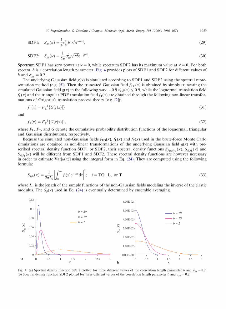
Spectrum SDF1 has zero power at j = 0, while spectrum SDF2 has its maximum value at j = 0. For bothspectra, b is a correlation length parameter. Fig. 4 provides plots of SDF1 and SDF2 for different values ofb and rgg = 0.2.

The underlying Gaussian field g(x) is simulated according to SDF1 and SDF2 using the spectral repre-sentation method (e.g. [5]). Then the truncated Gaussian field fTG(x) is obtained by simply truncating thesimulated Gaussian field g(x) in the following way: �0.9 6 g(x) 6 0.9, while the lognormal translation fieldfL(x) and the triangular PDF translation field fT(x) are obtained through the following non-linear transfor-mations of Grigoriu�s translation process theory (e.g. [2]):

fLðxÞ ¼ F �1L fG½gðxÞ�g ð31Þ

and

fTðxÞ ¼ F �1T fG½gðxÞ�g; ð32Þ

where FL, FT, and G denote the cumulative probability distribution functions of the lognormal, triangularand Gaussian distributions, respectively.

Because the simulated non-Gaussian fields fTG(x), fL(x) and fT(x) used in the brute-force Monte Carlosimulations are obtained as non-linear transformations of the underlying Gaussian field g(x) with pre-scribed spectral density function SDF1 or SDF2, their spectral density functions SfTGfTGðjÞ, SfLfLðjÞ andSfTfTðjÞ will be different from SDF1 and SDF2. These spectral density functions are however necessaryin order to estimate Var[u(x)] using the integral form in Eq. (24). They are computed using the followingformula:

SfifiðjÞ ¼1

2pLx

Z Lx

0

fiðxÞe�ijx dx

��2

; i ¼ TG; L; or T ð33Þ

where Lx is the length of the sample functions of the non-Gaussian fields modeling the inverse of the elasticmodulus. The Sff(j) used in Eq. (24) is eventually determined by ensemble averaging.

0

0.02

0.04

0.06

0.08

0.1

0.12

0 3κ κ

b = 20

b = 10

b = 2

0.00E+00

1.00E-02

2.00E-02

3.00E-02

4.00E-02

5.00E-02

6.00E-02

0 0.5 1 1.5 2 2.5 3

S gg

()

b = 20

b = 10

b = 2

0.5 1 1.5 2 2.5b

κ

(a) Spectral density function SDF1 plotted for three different values of the correlation length parameter b and rgg = 0.2.ctral density function SDF2 plotted for three different values of the correlation length parameter b and rgg = 0.2.


For the truncated Gaussian field, Var[u(x = L/2)] is computed through brute-force Monte Carlo simu-lations for various values of the correlation length parameter b in SDF1 and SDF2, and five different valuesof the standard deviation rgg of the underlying Gaussian field g(x): rgg = 0.2, rgg = 0.4, rgg = 0.6, rgg = 0.8and rgg = 1.0. The corresponding standard deviations of the truncated Gaussian field fTG(x) are estimatedas: rfTGfTG ¼ 0:2, rfTGfTG ¼ 0:3925, rfTGfTG ¼ 0:5313, rfTGfTG ¼ 0:6184 and rfTGfTG ¼ 0:675, respectively.Var[u(x = L/2)] is also computed via the integration in Eq. (24) in conjunction with the FMCS procedureto estimate the variability response function. This computation is carried out with a sufficiently refined dis-cretization of the integrand in Eq. (24) to achieve a sufficiently high level of accuracy. Fig. 5(a) providesplots of Var[u(x = L/2)] as a function of rfTGfTG when SDF1 is used as the spectral density function ofthe underlying Gaussian field g(x). Three different values of the correlation length parameter b are consi-dered. Fig. 5(b) presents similar results for SDF2. Fig. 5(a) and (b) demonstrates that the values ofVar[u(x = L/2)] computed using the integration in Eq. (24) and through brute-force Monte Carlo simula-tions practically coincide, regardless of the value of the standard deviation used for modeling the inverse ofthe modulus of elasticity.

The evolution of the relative error between the values of Var[u(x = L/2)] computed using the aforemen-tioned two approaches is demonstrated in Fig. 6, by selecting two of the cases displayed in Fig. 5. Speci-fically, Fig. 6(a) presents the evolution of this error for SDF1 with b = 2 and rfTGfTG ¼ 0:6184, whileFig. 6(b) presents corresponding results for SDF2 with the same values for b and rfTGfTG . The evolutionof the relative error is plotted as a function of the number of samples in the brute-force Monte Carlo sim-ulations (denoted by Nsamp). Fig. 6(a) and (b) clearly indicates that the relative error approaches zero. Sim-ilar behavior of the relative error was observed in all cases considered. It is therefore claimed that the resultsof the aforementioned two approaches are identical in all cases considered in this study.

The same procedure is followed for the translation fields with lognormal and triangular PDFs.Var[u(x = L/2)] is again computed through brute-force Monte Carlo simulations using an underlyingGaussian field with spectral density functions SDF1 and SDF2. Different values are considered for the

0.00E+00

2.00E-06

4.00E-06

6.00E-06

8.00E-06

0.00 0.10 0.20 0.30 0.40 0.50 0.60 0.70 0.80

Var

[ u( x

=L

/2)]

b = 20

b = 10

b = 2

MCS

0.00E+00

1.50E-06

3.00E-06

4.50E-06

6.00E-06

0.00 0.10 0.20 0.30 0.40 0.50 0.60 0.70 0.80

Var

[ u( x

=L

/2)]

b = 20

b = 10

b = 2

MCS

a bσ fTG fTGσ fTG fTG

Fig. 5. (a) Variance of response displacement at x = L/2 for the beam shown in Fig. 2 as a function of the standard deviation rfTGfTG :Comparison of results from the integration of Eq. (24) and from brute-force Monte Carlo simulations (MCS). Plots correspond tothree different values of correlation length parameter b of spectral density function SDF1. The corresponding PDF is a truncatedGaussian. (b) Variance of response displacement at x = L/2 for the beam shown in Fig. 2 as a function of the standard deviationrfTGfTG : Comparison of results from the integration of Eq. (24) and from brute-force Monte Carlo simulations (MCS). Plots correspondto three different values of correlation length parameter b of spectral density function SDF2. The corresponding PDF is a truncatedGaussian.

0

0.2

0.4

0.6

0.8

1

1.2

1.4

1.6

0 1 2 3 4 5

Nsamp (in millions)

erro

r (%

)

0

0.2

0.4

0.6

0.8

1

1.2

1.4

1.6

1.8

0 1 2 3 4 5

erro

r (%

)a bNsamp (in millions)

Fig. 6. (a) Evolution of relative error for SDF1 with b = 2 and rfTGfTG ¼ 0:6184. (b) Evolution of relative error for SDF2 with b = 2and rfTGfTG ¼ 0:6184.


correlation length parameter b. Four different values are considered for the standard deviations rfLfL andrfTfT of stochastic fields fL(x) and fT(x) respectively. They are displayed in Tables 1 and 2 together with thecorresponding lower limits of the lognormal and triangular PDFs. Var[u(x = L/2)] is also computed via theintegration in Eq. (24) in conjunction with the FMCS procedure to estimate the variability response func-tion. Fig. 7(a) provides plots of Var[u(x = L/2)] as a function of rfLfL for the case of the lognormal trans-lation field, while Fig. 7(b) presents similar results for the case of the translation field with triangular PDF.As with Figs. 5(a) and 5(b), Figs. 7(a) and 7(b) demonstrate again that the values of Var[u(x = L/2)] com-puted using the integration in Eq. (24) and through brute-force Monte Carlo simulations practically coin-cide, regardless of the value of the standard deviation used for modeling the inverse of the modulus ofelasticity. As mentioned above, the evolution of the relative error in these two cases (lognormal and trian-gular PDF�s) is similar to that of the truncated Gaussian field (refer to Fig. 6).

The validity of the two assumptions of existence and independence (that have been considered to form aconjecture) has been demonstrated numerically in this section for a wide range of stochastic fields f(x).Although such a numerical demonstration does not constitute a formal mathematical proof, the results dis-played in Figs. 5 and 7 provide ‘‘very strong numerical evidence’’ for the validity of the conjecture.

Table 1Values of standard deviation rfLfL considered and corresponding lower bounds of the lognormal PDF

rfLfL 0.2 0.4 0.6 0.7Lower limit �0.40 �0.60 �0.80 �0.95

Table 2Values of standard deviation rfTfT considered and corresponding lower bounds of the triangular PDF

rfTfT 0.20 0.40 0.60 0.70Lower limit �0.28 �0.56 �0.85 �0.99

0.00E+00

1.00E-06

2.00E-06

3.00E-06

4.00E-06

5.00E-06

0.00 0.20 0.40 0.60 0.80

SDF1 with b = 10SDF1 with b = 2SDF2 with b = 10SDF2 with b = 2MCS

0.00E+00

1.50E-06

3.00E-06

4.50E-06

6.00E-06

0.00 0.20 0.40 0.60 0.80

Var

[u(x

=L

/2)]

fL fLfL fL

Var

[u(x

=L

/2)]


a bσ σ

Fig. 7. (a) Variance of response displacement at x = L/2 for the beam shown in Fig. 2 as a function of the standard deviation rfLfL :Comparison of results from the integration of Eq. (24) and from brute-force Monte Carlo simulations (MCS). Plots correspond to twovalues of correlation length parameter b of spectral density functions SDF1 and SDF2. The corresponding PDF is a lognormal. (b)Variance of response displacement at x = L/2 for the beam shown in Fig. 2 as a function of the standard deviation rfTfT : Comparisonof results from the integration of Eq. (24) and from brute-force Monte Carlo simulations (MCS). Plots correspond to two values ofcorrelation length parameter b of spectral density functions SDF1 and SDF2. The corresponding PDF is triangular.


3.2.2. Limitation in FMCS procedure

The following limitation is implied when the Fast Monte Carlo Simulation procedure is used to estimatethe variability response function: as the flexibility cannot become negative at any point of the structure, thestandard deviation rff of the random sinusoids modeling the inverse of the elastic modulus cannot exceedthe value of 1=

ffiffiffi2

p(refer to Eq. (27)). For values greater than this limit, FMCS cannot be applied in the

form presented in this paper, as this will result in negative values of the flexibility. Although extendingthe applicability of FMCS beyond this limiting value of rff is beyond the scope of this paper, the followinggeneral concept is provided here: it is believed that for values of rff larger than 1=

ffiffiffi2

p, the random sinusoid

should be replaced with a zero mean field taking only positive values and having a spectral density functionas close as possible to the delta-function SDF of the corresponding random sinusoid (at the desired wavenumber). The full development of this concept is the subject of future research.

3.2.3. Closed-form expression for the variability response function in Eq. (26)

An important consequence of the validity of the two assumptions mentioned in the previous section isthat the VRF(x,j,rff) in Eq. (26) can be computed using the fast Monte Carlo simulation (FMCS) ap-proach described earlier. There is no need therefore for establishing closed-form analytic expressions forA�(x,j), A��(x,j) and A��(x,j) in Eq. (26). Although this is true, it will be demonstrated now how to ob-tain such closed-form analytic expressions in order to show that the VRF(x,j,rff) is indeed a function of rffas claimed earlier and as demonstrated numerically in Fig. 3.

To accomplish this, Eq. (22) is rewritten in the following way:

Rfpðx1; x2Þ ¼Z 1

�1Bðx1; x2; jÞSff ðjÞdj; ð34Þ

where

Bðx1; x2; jÞ ¼ A��ðx2; jÞ cos½jðx2 � x1Þ� þ A��ðx2; jÞ sin½jðx2 � x1Þ� ð35Þ
is an even function of j.


Closed-form analytic expressions for A�(x,j) and B(x1,x2,j) can be obtained now by assuming thatstochastic field f(x) in Eqs. (17) and (34) becomes a random sinusoid at wave number �j:

f ðxÞ ¼ffiffiffi2

prff cosð�jxþ /Þ ð36Þ

with corresponding spectral density function a delta function at �j:

Sff ðjÞ ¼ r2ff dðj� �jÞ. ð37Þ

This operation on Eqs. (17) and (34) yields the following expressions for j ¼ �j:

A�ðx1; jÞA�ðx2; jÞ ¼1

r2ff

½Rppðx1; x2Þ�jeijðx1�x2Þ

; ð38Þ

Bðx1; x2; jÞ ¼1

r2ff

½Rfpðx1; x2Þ�j; ð39Þ

where [Rpp(x1,x2)]j and [Rfp(x1,x2)]j denote the autocorrelation and cross-correlation functions Rpp(x1,x2)and Rfp(x1,x2) evaluated when stochastic field f(x) becomes a random sinusoid. Considering the expressionsin Eqs. (36) and (11), it is straightforward to show that:

A�ðx; jÞ ¼ 1

rffe½R2

jð1þffiffiffi2

prff cosðjxþ /ÞÞ2� � e½Rjð1þ

ffiffiffi2

prff cosðjxþ /ÞÞ�2

n o; ð40Þ

Bðx1; x2; jÞ ¼1

r2ff

e½Rj

ffiffiffi2

prff cosðjx1 þ /Þ� þ e½2Rjr

2ff cosðjx1 þ /Þ cosðjx2 þ /Þ�

n o; ð41Þ

where Rj denotes the redundant force defined in Eq. (8) for the particular case considered here involvingstochastic field f(x) as a random sinusoid:

Rj ¼

Q0

2

Z L

0

ðL� nÞ3ð1þffiffiffi2

prff cosðjnþ /ÞÞdnZ L

0

ðL� nÞ2ð1þffiffiffi2

prff cosðjnþ /ÞÞdn

. ð42Þ

The only uncertain quantity involved in the expectations shown in Eqs. (40) and (41) is the random phaseangle / that is uniformly distributed in the range [0,2p]. It is therefore possible to establish closed-formanalytic expressions for A�(x,j) and B(x1,x2,j) using any symbolic algebra software. The resulting expres-sions are very complicated and for this reason are not provided here. However, it is obvious that the result-ing expressions for A�(x,j) and B(x1,x2,j) will be functions of the standard deviation rff of stochastic fieldf(x) and of the (deterministic) geometry, loading and boundary conditions of the beam (note that theexpressions for A�(x,j) and B(x1,x2,j) will be independent of the random phase angle /, since the evalu-ation of the expectations in Eqs. (40) and (41) involves integration with respect to /). Finally, it should bementioned that the establishment of Eqs. (38)–(41) is based on the assumption that A�(x,j) and B(x1,x2,j)are independent from Sff(j).

3.3. Generality of integral expression in Eq. (24)

Whether the variability response function (VRF) is computed from the closed-form expressions in Eqs.(26), (35), (40) and (41), or using the fast Monte Carlo simulation (FMCS) approach, it should be men-tioned that there were no first-order approximations made whatsoever. Furthermore, similar closed-formexpressions can be established in principle for any statically indeterminate beam/frame with any kind ofboundary and loading conditions, as far as it can be analysed using a flexibility-based formulation similarto the one in Eq. (6) (with no limitation in the number of redundant forces). As such closed-form expres-


sions for the VRF become exceedingly complicated as the number of redundant forces increases, the VRF isusually computed using the FMCS approach.

4. Upper bounds on response variability

Using Eq. (4), upper bounds on the response displacement variance of a statically determinate beam canbe established in a straightforward way as follows:


�1VRFðx; jÞSff ðjÞdj 6 VRFðx; jmaxÞr2

ff ; ð43Þ

where jmax is the wave number at which the VRF takes its maximum value, and r2ff is the variance of sto-

chastic field f(x) modeling the inverse of the elastic modulus. Eq. (24) is used to determine the correspond-ing bounds for statically indeterminate beams:


�1VRFðx; j; rff ÞSff ðjÞdj 6 VRFðx; jmax; rff Þr2

ff ; ð44Þ

where jmax is the wave number at which the VRF corresponding to a given value of rff takes its maximumvalue, and r2

ff is the variance of stochastic field f(x) modeling the inverse of the elastic modulus.The upper bounds shown in Eqs. (43) and (44) are physically realizable since the form of stochastic field

f(x) that produces them is known. Specifically, the variance of u(x) attains its maximum value when randomfield f(x) becomes a random sinusoid:

f ðxÞ ¼ffiffiffi2

prff cosðjmaxxþ /Þ; ð45Þ

where / is a random phase angle uniformly distributed in [0,2p]. In this case, the corresponding spectraldensity function of f(x) is a delta function at wave number jmax:

Sff ðjÞ ¼ r2ff dðj� jmaxÞ; ð46Þ

while its PDF is a beta probability distribution function given by:

pf ðsÞ ¼1

pffiffiffiffiffiffiffiffiffiffiffiffiffiffiffiffiffiffi2r2

ff � s2q with�

ffiffiffi2

prff 6 s 6

ffiffiffi2

prff . ð47Þ

The upper bounds shown in Eqs. (43) and (44) are spectral- and probability-distribution-free, as the onlyprobabilistic parameter they depend on is the standard deviation of the inverse of the elastic modulus.

4.1. Bound generating fields

The concept of bound generating fields was introduced in [3]. It is summarized here as it will be used laterin the numerical examples section.

Whether a statically determinate or indeterminate beam is considered, the variance of the response dis-placement attains its maximum value when random field f(x) becomes a random sinusoid (Eq. (45)). Con-sequently, the following expression can be written for the inverse of the elastic modulus that produces theupper bounds:

1

EðxÞ ¼ F 0½1þ f ðxÞ� ¼ F 0½1þffiffiffi2

prff cosðjmaxxþ /Þ�. ð48Þ

A new stochastic field f �(x) modeling the elastic modulus and corresponding to stochastic field f(x) mod-eling the inverse of the elastic modulus can be defined now for this case that produces the upper bounds:


EðxÞ ¼ 1

F 0

1

½1þ f ðxÞ� ¼ E0½1þ f �ðxÞ�; ð49Þ

where E0 is the mean value of the elastic modulus which is related to F0 via:

E0 ¼1

F 0

e1

ð1þ f ðxÞÞ

� �ð50Þ

f �(x) is a zero-mean, homogeneous stochastic field related to f(x) through the following relationship:

f �ðxÞ ¼1� e

1

ð1þ f ðxÞÞ

� �ð1þ f ðxÞÞ

e1

ð1þ f ðxÞÞ

� �ð1þ f ðxÞÞ

. ð51Þ

Stochastic field f �(x) is called a bound generating field (BGF) since it produces realizable upper bounds.Sample functions of f �(x) can be easily obtained from generated realizations of the random sinusoid f(x)using Eq. (51). A closed-form analytic expression for the PDF of f �(x) is available, and its spectral densityfunction can be easily estimated from generated sample functions of f �(x) (refer to [3] for a detailed descrip-tion of BGFs and their properties).

4.2. Three alternative ways to perform fast Monte Carlo simulation

Eq. (51) indicates that when random field f(x) modeling the inverse of the elastic modulus is a randomsinusoid, random field f �(x) modeling the elastic modulus can be fully determined, i.e. a sample function off �(x) can be computed from a given sample function of f(x). Consequently, there are essentially three alter-native ways to perform the fast Monte Carlo simulation to estimate Var½uðxÞ��j in Eq. (28):

1. By generating sample functions of f(x) (in this case a random sinusoid) and then using a closed-formanalytic expression for the response displacement (Eq. (7)). This approach is called ANA � f(x).

2. By generating sample functions of f(x) (in this case a random sinusoid), computing the correspondingsample functions of f �(x) using Eq. (51), and then using a closed-form analytic expression for theresponse displacement. This approach is called ANA � f �(x).

3. By generating sample functions of f(x) (in this case a random sinusoid), computing the correspondingsample functions of f �(x) using Eq. (51), and then using a deterministic finite element code to estimatethe response displacement. This approach is called FEM � f �(x).

It is obvious that the third approach is not requiring the existence of a closed-form analytic expression forthe response displacement. All three approaches provide identical estimates of Var½uðxÞ��j (and consequentlyof the variability response function too).

At this juncture, it should be mentioned that although in the case of statically determinate beams thevariability response function can be computed from the closed-form analytic expression shown in Eq.(5), alternatively, the VRF(x,j) can also be estimated using the fast Monte Carlo simulation approach de-scribed earlier for statically indeterminate beams. This is very helpful in cases where function g(x,n) of thestatically determinate problem becomes too cumbersome.

5. Numerical examples

Example 1. Consider again the fixed-simply supported beam of length L = 10 m shown in Fig. 2. Two loadcases are considered: LC1 consisting of a uniformly distributed load Q0 = 1000 N/m and LC2 consisting of


the same uniformly distributed load Q0 = 1000 N/m and a concentrated moment M0 = �10,000 Nmapplied at its right end (please note that this concentrated moment is not indicated in Fig. 2). All loads areassumed again to be deterministic. The inverse of the elastic modulus of the beam is assumed to varyrandomly along its length according to Eq. (1) with F0 = 8 · 10�9 m2/N and I = 0.1 m4.

5.1. Analysis of response variability

For LC1, an extensive numerical investigation was performed in section ‘‘Demonstration of the validity of

the assumptions of existence and independence’’ where Var[u(x = L/2)] was estimated using the integration inEq. (24) in conjunction with the ANA � f(x) technique for calculating the VRF, and through brute-forceMonte Carlo simulations. As can be observed in Figs. 5–7, the two approaches produced practically iden-tical results in all cases considered.

The same procedure is followed now for LC2. Fig. 8 displays plots of VRF(x = 3L/4,j,rff) calculatedusing the ANA � f(x) approach for various values of the standard deviation rff. As with LC1 (Fig. 3),Fig. 8 indicates that the VRF of LC2 is again a function of the standard deviation rff, while the differencesobserved among the different VRF curves obtained for the four values of rff considered are relatively small(and become negligible for rff < 0.4). Numerical results for LC2 are obtained for a truncated Gaussian fieldonly (having the same definition as before). Fig. 9 provides plots of Var[u(x = 3L/4)] as a function of rfTGfTG

when SDF1 and SDF2 are used as the spectral density function of the underlying Gaussian field g(x). Twodifferent values of the correlation length parameter b are considered. Fig. 9 indicates that the values ofVar[u(x = 3L/4)] computed using the integration in Eq. (24) and through brute-force Monte Carlo simula-tions practically coincide, regardless of the value of the standard deviation used for modeling the inverse ofthe modulus of elasticity. The evolution of the relative error for LC2 is similar to that shown in Fig. 6.

The variance of the response displacement can be calculated with minimal computational effort using theintegration in Eq. (24) for prescribed forms of the spectral density function Sff(j). Fig. 10(a) and (b) dis-plays results of such calculations for LC1 and LC2 respectively. SDF1 and SDF2 are used to model Sff(j)with standard deviation rff = 0.4. The computed results are plotted as a function of correlation distanceparameter b.

5.1.1. Spectral- and probability-distribution-free upper bounds

Spectral- and probability-distribution-free upper bounds for the variance of the response displacementare computed now using Eq. (44). For LC1, upper bounds are determined for Var[u(x = L/2)] for variousvalues of the standard deviation rff of the inverse of the elastic modulus:

0.00E+00

5.00E-07

1.00E-06

1.50E-06

0 0.5 1 1.5κ

2 2.5 3

VR

F(x=

3L/4

, ,

ff) σ ff = 0.2

σ ff = 0.4σ ff = 0.6σ ff = 0.7

κσ

Fig. 8. Variability response function calculated using the FMCS approach for the beam in Example 1 and for LC2. Four differentvalues rff are considered.

0.00E+00

1.00E-07

2.00E-07

3.00E-07

4.00E-07

5.00E-07

0.00 0.10 0.20 0.30 0.40 0.50 0.60 0.70 0.80

Var

[u(x

=3L

/4)]


TG TGf fσ

Fig. 9. Example 1 and LC2: Variance of response displacement at x = 3L/4 as a function of standard deviation rfTGfTG : Comparison ofresults from the integration of Eq. (24) and from brute-force Monte Carlo simulations (MCS). Plots correspond to two values ofcorrelation length parameter b of spectral density functions SDF1 and SDF2. The corresponding PDF is a truncated Gaussian.

0.00E+00

1.00E-06

2.00E-06

3.00E-06

0 5 10 15 20 25 30 35 40b

Var

[u(x

=L

/2)]

SDF1

SDF2

0.00E+00

5.00E-08

1.00E-07

1.50E-07

0 5 10 15 20 25 30 35 40b

Var

[u(x

=3L

/4)]

SDF1

SDF2

a b

Fig. 10. (a) Example 1 and LC1: Variance of response displacement at x = L/2 calculated through the integration in Eq. (24) and usingSDF1 and SDF2 to model the spectral density function Sff(j). Both curves are established for rff = 0.4 and plotted as a function ofcorrelation length parameter b. (b) Example 1 and LC2: Variance of response displacement at x = L/2 calculated through theintegration in Eq. (24) and using SDF1 and SDF2 to model the spectral density function Sff(j). Both curves are established for rff = 0.4and plotted as a function of correlation length parameter b.


Var½uðx ¼ L=2Þ� 6 VRFðx ¼ L=2; jmax; rff ¼ 0:2Þ � 0:22 ¼ 7:00� 10�7; jmax ¼ 0; ð52Þ



Var½uðx ¼ L=2Þ� 6 VRFðx ¼ L=2; jmax; rff ¼ 0:7Þ � 0:72 ¼ 8:53� 10�6; jmax ¼ 0. ð55Þ


For LC2, upper bounds are determined for Var[u(x = 3L/4)]:

Fig. 12values

Var½uðx ¼ 3L=4Þ� 6 VRFðx ¼ 3L=4; jmax; rff ¼ 0:2Þ � 0:22 ¼ 5:56� 10�8; jmax ¼ 1:1; ð56ÞVar½uðx ¼ 3L=4Þ� 6 VRFðx ¼ 3L=4; jmax; rff ¼ 0:4Þ � 0:42 ¼ 2:24� 10�7; jmax ¼ 1:1; ð57ÞVar½uðx ¼ 3L=4Þ� 6 VRFðx ¼ 3L=4; jmax; rff ¼ 0:6Þ � 0:62 ¼ 5:09� 10�7; jmax ¼ 1:1; ð58ÞVar½uðx ¼ 3L=4Þ� 6 VRFðx ¼ 3L=4; jmax; rff ¼ 0:7Þ � 0:72 ¼ 7:01� 10�7; jmax ¼ 1:1. ð59Þ

For LC1, the upper bounds shown in Eqs. (52)–(55) are obtained when stochastic field f(x) modeling theinverse of the elastic modulus degenerates into a random variable (as jmax = 0). For LC2, the upper boundsshown in Eqs. (56)–(59) are obtained when stochastic field f(x) becomes a random sinusoid with wave num-ber jmax = 1.1. In this case, the bound generating field f �(x) modelling the elastic modulus can be easilydetermined from Eq. (51).

Example 2. Consider now the twice-statically-indeterminate fixed beam of length L = 10 m shown inFig. 11. Two load cases are considered in this example: LC1 consisting of a concentrated forceP0 = 10,000 N acting at the midspan (x = L/2), and LC2 consisting of the same concentrated forceP0 = 10,000 N and a concentrated moment M0 = 10,000 N m acting also at x = L/2 (please note that thisconcentrated moment is not indicated in Fig. 2). All loads are assumed again to be deterministic. Theinverse of the elastic modulus of the beam is assumed to vary randomly along its length according to Eq. (1)with F0 = 8 · 10�9 m2/N and I = 0.1 m4.


The same procedure as in Example 1 is followed here. Fig. 12 displays plots of VRF(x = 3L/4,j,rff) cal-culated using the FEM � f �(x) approach for LC1, while Fig. 13 displays similar plots for LC2. For the

Fig. 11. Configuration of fixed statically indeterminate beam.

0.00E+00

5.00E-06

1.00E-05

1.50E-05

2.00E-05

0 1.5 2κ

0.5 1

VR

F(x

=L

/2,κ

σ ,ff)

σ ff = 0.2

σ ff = 0.4

σ ff = 0.6

σ ff = 0.7

. Variability response function calculated using the FMCS approach for the beam in Example 2 and for LC1. Four differentrff are considered.

0.00E+00

2.00E-06

4.00E-06

6.00E-06

0 0.5 1 1.5 2κ

VR

F(x

=3L

/4,κ

σ ,ff)

σ ff = 0.2

σ ff = 0.4

σ ff = 0.6

σ ff = 0.7

Fig. 13. Variability response function calculated using the FMCS approach for the beam in Example 2 and for LC2. Four differentvalues rff are considered.


FEM analysis, the beam is discretized into 100 finite elements. As in Example 1, Figs. 12 and 13 indicatethat the VRF is again a function of rff, while the differences observed among the four VRF curves obtainedfor the four values of rff considered are relatively small (and become negligible for rff < 0.4). In this exam-ple, only the truncated Gaussian field is considered (having the same definition as before). Fig. 14 providesplots of Var[u(x = L/2)] for LC1 as a function of rfTGfTG when SDF1 and SDF2 are used as the spectraldensity function of the underlying Gaussian field g(x). Two different values of the correlation length para-meter b are considered. Fig. 15 provides similar plots for Var[u(x = 3L/4)] and LC2. Figs. 14 and 15 indi-cate that the values for the variance of the response displacement computed using the integration in Eq. (24)and through brute-force Monte Carlo simulations practically coincide, regardless of the value of the stan-dard deviation used for modeling the inverse of the modulus of elasticity. The evolution of the relative errorfor both LC1 and LC2 is similar to that shown in Fig. 6.

Fig. 16(a) and (b) displays results for Var[u(x = L/2)] and Var[u(x = 3L/4)] corresponding to LC1 andLC2, respectively, calculated using the integration in Eq. (24). SDF1 and SDF2 are used to model Sff(j)

0.00E+00

1.00E-06

2.00E-06

3.00E-06

4.00E-06

5.00E-06

0.00 0.10 0.20 0.30 0.40 0.50 0.60 0.70 0.80

Var

[u(x

=L

/2)]


TG TGf fσ

Fig. 14. Example 2 and LC1: Variance of response displacement at x = L/2 as a function of standard deviation rfTGfTG : Comparison ofresults from the integration of Eq. (24) and from brute-force Monte Carlo simulations (MCS). Plots correspond to two values ofcorrelation length parameter b of spectral density functions SDF1 and SDF2. The corresponding PDF is a truncated Gaussian.

0.00E+00

2.50E-07

5.00E-07

7.50E-07

1.00E-06

1.25E-06

1.50E-06

0.00 0.10 0.20 0.30 0.40 0.50 0.60 0.70 0.80

Var

[u(x

=3L

/4)]


TG TGf fσ

Fig. 15. Example 2 and LC2: Variance of response displacement at x = 3L/4 as a function of standard deviation rfTGfTG : Comparisonof results from the integration of Eq. (24) and from brute-force Monte Carlo simulations (MCS). Plots correspond to two values ofcorrelation length parameter b of spectral density functions SDF1 and SDF2. The corresponding PDF is a truncated Gaussian.

0.00E+00

1.00E-06

2.00E-06

3.00E-06

0 5 10 15 20 25 30 35 40b

Var

[u(x

=L

/2)]

SDF1

SDF2

a

0.00E+00

2.00E-07

4.00E-07

6.00E-07

8.00E-07

0 5 10 15 20 25 30 35 40b

Var

[u(x

=3L

/4)]

SDF1

SDF2

b

Fig. 16. (a) Example 2 and LC1: Variance of response displacement at x = L/2 calculated through the integration in Eq. (24) and usingSDF1 and SDF2 to model the spectral density function Sff(j). Both curves are established for rff = 0.4 and plotted as a function ofcorrelation length parameter b. (b) Example 2 and LC2: Variance of response displacement at x = 3L/4 calculated through theintegration in Eq. (24) and using SDF1 and SDF2 to model the spectral density function Sff(j). Both curves are established for rff = 0.4and plotted as a function of correlation length parameter b.


with standard deviation rff = 0.4. The computed results are plotted as a function of correlation distanceparameter b.

5.2.1. Spectral- and probability-distribution-free upper boundsSpectral- and probability-distribution-free upper bounds for the variance of the response displacement

are computed now using Eq. (44). For LC1, upper bounds are determined for Var[u(x = L/2)] for variousvalues of the standard deviation rff of the inverse of the elastic modulus:


Var½uðx ¼ L=2Þ� 6 VRFðx ¼ L=2; jmax; rff ¼ 0:2Þ � 0:22 ¼ 6:92� 10�6; jmax ¼ 0; ð60ÞVar½uðx ¼ L=2Þ� 6 VRFðx ¼ L=2; jmax; rff ¼ 0:4Þ � 0:42 ¼ 2:77� 10�6; jmax ¼ 0; ð61ÞVar½uðx ¼ L=2Þ� 6 VRFðx ¼ L=2; jmax; rff ¼ 0:6Þ � 0:62 ¼ 6:20� 10�6; jmax ¼ 0; ð62ÞVar½uðx ¼ L=2Þ� 6 VRFðx ¼ L=2; jmax; rff ¼ 0:7Þ � 0:72 ¼ 8:48� 10�6; jmax ¼ 0. ð63Þ

For LC2, upper bounds are determined for Var[u(x = 3L/4)]:

Var½uðx ¼ 3L=4Þ� 6 VRFðx ¼ 3L=4; jmax; rff ¼ 0:2Þ � 0:22 ¼ 2:04� 10�7; jmax ¼ 0; ð64ÞVar½uðx ¼ 3L=4Þ� 6 VRFðx ¼ 3L=4; jmax; rff ¼ 0:4Þ � 0:42 ¼ 8:16� 10�7; jmax ¼ 0; ð65ÞVar½uðx ¼ 3L=4Þ� 6 VRFðx ¼ 3L=4; jmax; rff ¼ 0:6Þ � 0:62 ¼ 1:83� 10�6; jmax ¼ 0; ð66ÞVar½uðx ¼ 3L=4Þ� 6 VRFðx ¼ 3L=4; jmax; rff ¼ 0:7Þ � 0:72 ¼ 2:50� 10�6; jmax ¼ 0. ð67Þ

For both LC1 and LC2, the upper bounds shown in Eqs. (60)–(67) are obtained when stochastic field f(x)modeling the inverse of the elastic modulus degenerates into a random variable (as jmax = 0).

Example 3. Consider finally the statically indeterminate portal plane frame shown in Fig. 17 with L = 4 m.The two base nodes are assumed fixed against translations and rotations. The loading consists of adeterministic horizontal force equal to P0 = 10,000 N applied at node A (refer to Fig. 17). The inverse ofthe elastic modulus of the frame is assumed to vary randomly along its length according to Eq. (1) withF0 = 8 · 10�9 m2/N and I = 0.1 m4.


The same procedure as in Examples 1 and 2 is also followed here. Denoting by uAhthe horizontal dis-

placement of node A and by VRFAhðj; rff Þ the corresponding variability response function, Fig. 18 dis-

plays plots of VRFAhðj; rff Þ calculated using the FEM � f �(x) approach. For the FEM analysis, the

frame is discretized into 120 finite elements. As in Examples 1 and 2, Fig. 18 indicates that the VRF is againa function of rff, while the differences observed among the four VRF curves obtained for the four values ofrff considered are relatively small (and become negligible for rff < 0.4). In this example, only the truncatedGaussian field is considered with SDF1 and b = 2. Fig. 19 provides plots of VarðuAh

Þ as a function ofrfTGfTG . Fig. 19 indicates that the values for the variance of the response displacement computed using

Fig. 17. Portal frame considered in Example 3.

0.00E+00

5.00E-06

1.00E-05

1.50E-05

2.00E-05

2.50E-05

0 1 2 4κ

VR

F Ah

( κ σ

,

ff)

3 5

σ

σ

σ

σ

ff = 0.2

ff = 0.4

ff = 0.6

ff = 0.7

Fig. 18. Variability response function calculated using the FMCS approach for the portal frame in Example 3. Four different values rffare considered.

0.00E+00

3.00E-07

6.00E-07

9.00E-07

1.20E-06

1.50E-06

0.00 0.20 0.40 0.60 0.80

Var

(uA

h)

SDF1 with b = 2

MCS

TG TGf fσ

Fig. 19. Example 3: Variance of response displacement uAhas a function of standard deviation rfTGfTG : Comparison of results from the

integration of Eq. (24) and from brute-force Monte Carlo simulations (MCS). Plots correspond to a correlation length parameter b = 2of spectral density function SDF1. The corresponding PDF is a truncated Gaussian.


the integration in Eq. (24) and through brute-force Monte Carlo simulations practically coincide, regardlessof the value of the standard deviation used for modeling the inverse of the modulus of elasticity. The evo-lution of the relative error is similar to that shown in Fig. 6. Fig. 20 displays results for VarðuAh

Þ calculatedusing the integration in Eq. (24). SDF1 is used to model Sff(j) with standard deviation rff = 0.4. The com-puted results are plotted as a function of correlation distance parameter b.

Figs. 10, 16 and 20 provide information about the behavior of the variance of the response displacementover the entire range of values of the correlation length parameter of the spectral density function consid-ered. With other available methodologies, the corresponding calculations would require a significant com-putational effort. The concept of the variability response function not only makes the computational efforttrivial, but it also provides an excellent insight on the effect of the shape of Sff(j) through the integral formin Eq. (24).

0.00E+00

1.00E-06

2.00E-06

3.00E-06

4.00E-06

0 5 10 15 20 25 30 35 40b

Var

(u A

h)SDF1

Fig. 20. Example 3: Variance of response displacement uAhcalculated through the integration in Eq. (24) and using SDF1 to model the

spectral density function Sff(j). Curve is established for rff = 0.4 and plotted as a function of correlation length parameter b.


5.3.1. Spectral- and probability-distribution-free upper bounds

Spectral- and probability-distribution-free upper bounds for the variance of the response displacementare computed now using Eq. (44). Upper bounds are determined for VarðuAh

Þ for various values of the stan-dard deviation rff of the inverse of the elastic modulus:

VarðuAhÞ 6 VRFAh

ðjmax; rff ¼ 0:2Þ � 0:22 ¼ 8:81� 10�7; jmax ¼ 0; ð68ÞVarðuAh

Þ 6 VRFAhðjmax; rff ¼ 0:4Þ � 0:42 ¼ 3:53� 10�6; jmax ¼ 0; ð69Þ

VarðuAhÞ 6 VRFAh

ðjmax; rff ¼ 0:6Þ � 0:62 ¼ 7:92� 10�6; jmax ¼ 0; ð70ÞVarðuAh

Þ 6 VRFAhðjmax; rff ¼ 0:7Þ � 0:72 ¼ 1:08� 10�5; jmax ¼ 0. ð71Þ

6. Conclusions

The present paper complemented and extended work done in an earlier study of the authors [3] dealingwith the analysis of the response variability of stochastic frame structures. The well-known integral formfor the response displacement variance was established in this paper for statically indeterminate structuresusing a different formulation (applying the concept of non-homogeneous evolutionary fields) that involvedan alternative conjecture. The validation of the conjecture was done by comparing the response variancepredictions of the integral form with Monte Carlo simulations.

A methodology was provided to determine the variability response function (VRF) (involved in the inte-gral form) numerically through a so-called fast Monte Carlo simulation (FMCS) technique. In addition,closed-form expressions were established for the VRF that indicate a dependence on the standard deviationof the stochastic field modeling the inverse of the elastic modulus, a fact that was validated numericallythrough the FMCS technique.

Several numerical examples were provided estimating the variance of the response displacement usingthe integral form in Eq. (24) (in conjunction with a FMCS computation of the VRF) and throughbrute-force Monte Carlo simulations. The results of the two approaches practically coincided for all casesconsidered (validating the aforementioned conjecture). Additional numerical examples demonstrated theexcellent insight on the effect of the form of the spectral density function of the stochastic field modelingthe inverse of the elastic modulus on the response variability. Finally, upper bounds were provided for sev-eral cases as a function of the standard deviation of the stochastic field modeling the inverse of the elasticmodulus. All computations involving Eq. (24) (determining variance of response and upper bounds) werecarried out with minimal computational effort.


Acknowledgements

This work was supported by the National Science Foundation under Grant # CMS-01-15901, with Dr.Peter Chang as Program Director.

References

[1] I. Elishakoff, Y.J. Ren, M. Shinozuka, Some exact solutions for the bending of beams with spatially stochastic stiffness, Int. J.Solids Struct. 32 (16) (1995) 2315–2327.

[2] M. Grigoriu, Applied Non-Gaussian Processes: Examples, Theory, Simulation, Linear Random Vibration, and MATLABSolutions, Prentice Hall, 1995.

[3] V. Papadopoulos, G. Deodatis, M. Papadrakakis, Flexibility-based upper bounds on the response variability of simple beams,Comput. Methods Appl. Mech. Engrg. 194 (12–16) (2005) 1385–1404.

[4] M.B. Priestley, Non-linear and Non-stationary Time Series Analysis, Academic Press, 1988.[5] M. Shinozuka, G. Deodatis, Simulation of stochastic processes by spectral representation, Appl. Mech. Rev. 44 (4) (1991) 191–203.

Documents

Response variability of stochastic frame structures …users.ntua.gr/vpapado/Publications/Publication8.pdfResponse variability of stochastic frame structures using evolutionary ﬁeld