Response of Jupiter’s auroras to conditions in the

Confidential manuscript submitted to Geophysical Research Letters

Response of Jupiter’s auroras to conditions in the interplanetary

medium as measured by the Hubble Space Telescope and Juno

J. D. Nichols1, S. V. Badman2, F. Bagenal3, S. J. Bolton4, B. Bonfond5, E. J. Bunce1, J. T.

Clarke6, J. E. P. Connerney7, S. W. H. Cowley1, R. W. Ebert4, M. Fujimoto8, J.-C. Gérard5,

G. R. Gladstone4, D. Grodent5, T. Kimura9, W. S. Kurth10, B. H. Mauk11, G. Murakami12, D.

J. McComas13, G. S. Orton14, A. Radioti5, T. S. Stallard1, C. Tao15, P. W. Valek4, R. J.

Wilson3, A. Yamazaki12, I. Yoshikawa16

1Department of Physics and Astronomy, University of Leicester, University Road, Leicester, LE1 7RH, UK2Department of Physics, Lancaster University, LA1 4YB, UK

3Laboratory for Atmospheric and Space Physics, University of Colorado Boulder, Boulder, Colorado, USA4Southwest Research Institute, San Antonio, Texas, USA

5Laboratory for Planetary and Atmospheric Physics, Université de Liège, Institut d’Astrophysique et de Géophysique - B5c,

Allée du 6 aout, 17, B-4000 Liége, Belgium6725 Commonwealth Avenue, Center for Space Physics, Boston University, Boston, MA 02215, USA

7Goddard Space Flight Center, Greenbelt, Maryland, USA8Institute of Space and Astronautical Science, Japan Aerospace Exploration Agency, Sagamihara, Japan

9Nishina Center for Accelerator-Based Science, RIKEN, RIBF403, 2-1, Hirosawa, Saitama,Japan10Department of Physics and Astronomy, University of Iowa, Iowa City, IA 52241, USA

11Johns Hopkins University Applied Physics Laboratory, 11100 Johns Hopkins Road, Laurel, MD 20723, USA12Institute of Space and Astronautical Science, Japan Aerospace Exploration Agency, Sagamihara, Japan

13Princeton Plasma Physics Laboratory, P.O. Box 451, Princeton, NJ 08543-0451, USA14Jet Propulsion Laboratory, M/S 169-237 , 4800 Oak Grove Drive , Pasadena, CA 91109, USA

15Space Environment Laboratory, National Institute of Information and Communications Technology, Tokyo, Japan16Department of Complexity Science and Engineering, University of Tokyo, Kashiwa, Japan

Key Points:

• We present the first comparison of Jupiter’s auroras with an extended and completeset of near-Jupiter interplanetary data.

• During compressions, the well-defined sector of Jupiter’s emission and the duskpoleward region brightened, the latter pulsating.

• The power emitted from the noon active region did not exhibit dependence on anyinterplanetary parameter, though the morphology changed.

Corresponding author: J. D. Nichols, [email protected]

–1–


Abstract

We present the first comparison of Jupiter’s auroral morphology with an extended, con-tinuous and complete set of near-Jupiter interplanetary data, revealing the response ofJupiter’s auroras to the interplanetary conditions. We show that for ∼1-3 days followingcompression region onset the planet’s main emission brightened. A duskside poleward re-gion also brightened during compressions, as well as during shallow rarefaction conditionsat the start of the program. The power emitted from the noon active region did not exhibitdependence on any interplanetary parameter, though the morphology typically differedbetween rarefactions and compressions. The auroras equatorward of the main emissionbrightened over ∼10 days following an interval of increased volcanic activity on Io. Theseresults show that the dependence of Jupiter’s magnetosphere and auroras on the interplan-etary conditions are more diverse than previously thought.

1 Introduction

The dynamics of Jupiter’s magnetosphere are dominated by planetary rotation andthe outflow of material from Io [see e.g. Khurana et al., 2004; Clarke et al., 2004], andthe nature of the solar wind interaction has long been debated [Brice and Ioannidis, 1970;Southwood and Kivelson, 2001; Nichols et al., 2006; Badman and Cowley, 2007; McComas

and Bagenal, 2007; Cowley et al., 2008; Delamere and Bagenal, 2010]. Observationally,the total power of the jovian auroras in various wavelengths exhibits modulation by inter-planetary conditions [Baron et al., 1996; Pryor et al., 2005; Clarke et al., 2009; Badman

et al., 2016; Kita et al., 2016; Kimura et al., 2016; Dunn et al., 2016], particularly increas-ing in some cases (not all) in response to expected solar wind compression regions charac-terised by overall high dynamic pressure and interplanetary magnetic field (IMF) strength.

The detailed morphological response of the far-ultraviolet auroras to the interplane-tary medium has been examined previously using the Hubble Space Telescope (HST) andnear-Jupiter spacecraft by Nichols et al. [2007, 2009a], the former study comparing HSTimages with Cassini flyby observations, and the latter with New Horizons solar wind dataand interplanetary measurements extrapolated from Earth orbit using a magnetohydro-dynamic model. These studies showed that in response to expected compression regiononset the main emission sometimes brightened in the narrow region with System III lon-gitude λ I I I >180◦ (usually observed in the dawn sector by HST), whereas, in contrast theemission at smaller longitudes was neither bright nor well-defined. However, intense arcspoleward of the main emission were observed during estimated compression regions foraround 2 days following estimated compression region onset. An important limitation ofthose studies, however, was that they were hampered by relying on either limited HST orinterplanetary observations, or interplanetary data extrapolated from Earth that carried sig-nificant timing uncertainties. Further, those HST observations were obtained using eitherfixed ∼100 s exposure times, or time-tag exposures of less than 5 minutes, both of whichlimit characterisation of fast-varying auroral forms. In 2016 the NASA Juno spacecraft ap-proached and entered into orbit around Jupiter (with orbit insertion on 5 July 2016), pro-viding a full and continuous complement of near-Jupiter solar wind and IMF data. Duringthis interval we observed Jupiter’s FUV auroras using the HST Space Telescope ImagingSpectrograph (STIS) for 47 orbits from 16 May to 18 July, primarily using ∼45 min time-tag imaging exposures. In this paper we examine this unique combination of data in orderto determine the response of Jupiter’s auroras to conditions in the interplanetary medium.We show that Jupiter’s auroral response to interplanetary conditions is more diverse thanpreviously understood.

–2–


2 Data

2.1 Hubble Space Telescope observations

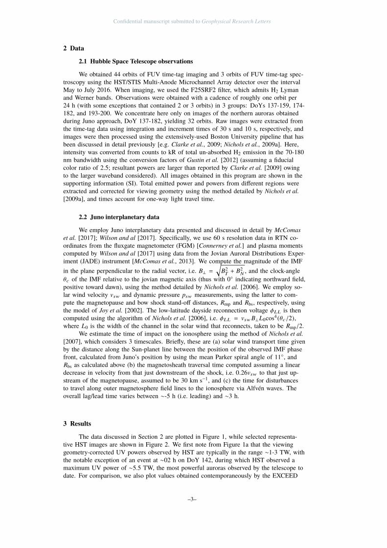
We obtained 44 orbits of FUV time-tag imaging and 3 orbits of FUV time-tag spec-troscopy using the HST/STIS Multi-Anode Microchannel Array detector over the intervalMay to July 2016. When imaging, we used the F25SRF2 filter, which admits H2 Lymanand Werner bands. Observations were obtained with a cadence of roughly one orbit per24 h (with some exceptions that contained 2 or 3 orbits) in 3 groups: DoYs 137-159, 174-182, and 193-200. We concentrate here only on images of the northern auroras obtainedduring Juno approach, DoY 137-182, yielding 32 orbits. Raw images were extracted fromthe time-tag data using integration and increment times of 30 s and 10 s, respectively, andimages were then processed using the extensively-used Boston University pipeline that hasbeen discussed in detail previously [e.g. Clarke et al., 2009; Nichols et al., 2009a]. Here,intensity was converted from counts to kR of total un-absorbed H2 emission in the 70-180nm bandwidth using the conversion factors of Gustin et al. [2012] (assuming a fiducialcolor ratio of 2.5; resultant powers are larger than reported by Clarke et al. [2009] owingto the larger waveband considered). All images obtained in this program are shown in thesupporting information (SI). Total emitted power and powers from different regions wereextracted and corrected for viewing geometry using the method detailed by Nichols et al.

[2009a], and times account for one-way light travel time.

2.2 Juno interplanetary data

We employ Juno interplanetary data presented and discussed in detail by McComas

et al. [2017]; Wilson and al [2017]. Specifically, we use 60 s resolution data in RTN co-ordinates from the fluxgate magnetometer (FGM) [Connerney et al.] and plasma momentscomputed by Wilson and al [2017] using data from the Jovian Auroral Distributions Exper-iment (JADE) instrument [McComas et al., 2013]. We compute the magnitude of the IMF

in the plane perpendicular to the radial vector, i.e. B⊥ =

√

B2T+ B2

N, and the clock-angle

θc of the IMF relative to the jovian magnetic axis (thus with 0◦ indicating northward field,positive toward dawn), using the method detailed by Nichols et al. [2006]. We employ so-lar wind velocity vsw and dynamic pressure psw measurements, using the latter to com-pute the magnetopause and bow shock stand-off distances, Rmp and Rbs, respectively, usingthe model of Joy et al. [2002]. The low-latitude dayside reconnection voltage φLL is thencomputed using the algorithm of Nichols et al. [2006], i.e. φLL = vswB⊥L0cos4(θc/2),where L0 is the width of the channel in the solar wind that reconnects, taken to be Rmp/2.

We estimate the time of impact on the ionosphere using the method of Nichols et al.

[2007], which considers 3 timescales. Briefly, these are (a) solar wind transport time givenby the distance along the Sun-planet line between the position of the observed IMF phasefront, calculated from Juno’s position by using the mean Parker spiral angle of 11◦, andRbs as calculated above (b) the magnetosheath traversal time computed assuming a lineardecrease in velocity from that just downstream of the shock, i.e. 0.26vsw to that just up-stream of the magnetopause, assumed to be 30 km s−1, and (c) the time for disturbancesto travel along outer magnetosphere field lines to the ionosphere via Alfvén waves. Theoverall lag/lead time varies between ∼-5 h (i.e. leading) and ∼3 h.

3 Results

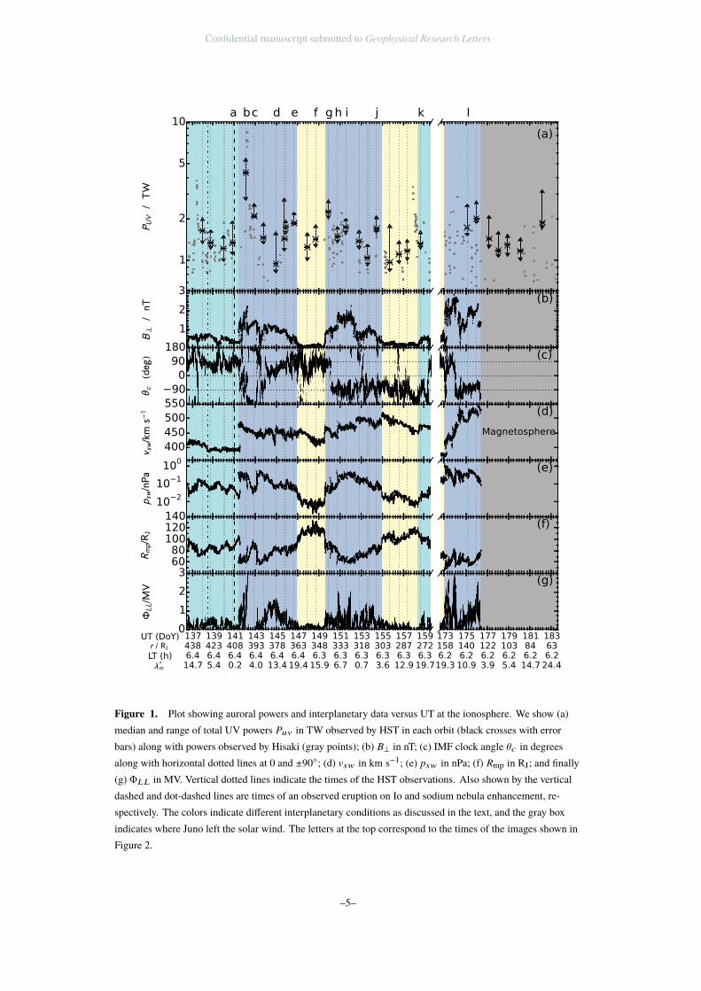
The data discussed in Section 2 are plotted in Figure 1, while selected representa-tive HST images are shown in Figure 2. We first note from Figure 1a that the viewinggeometry-corrected UV powers observed by HST are typically in the range ∼1-3 TW, withthe notable exception of an event at ∼02 h on DoY 142, during which HST observed amaximum UV power of ∼5.5 TW, the most powerful auroras observed by the telescope todate. For comparison, we also plot values obtained contemporaneously by the EXCEED

–3–


instrument on the JAXA Hisaki satellite, provided by Kimura and et al. [2017]. The Hisakipowers are also corrected for viewing geometry and scaled to the same bandwidth of theHST values (see Tao et al. [2016] for further information). Hisaki UV powers broadlyconcur with HST observations, though with increased temporal coverage which indicatedthat the power continued to rise still further on DoY 142 to ∼8.5 TW before droppingto ∼2.1 TW at the time of the second HST observation on DoY 142 at ∼2130 h. Othernotable enhancements of the total power up to values of ∼2 TW occurred on DoYs 146,151, 154, 175, 176, and 182, while a short-lived enhancement between HST orbits wasobserved by Hisaki on DoY 158.

The interplanetary data shown in Figures 1b-g indicates that the field was BT -dominatedas expected at ∼5 AU and that three solar wind compression regions were incident onJupiter’s magnetosphere during these intervals, separated by rarefaction regions of vary-ing depth. The first compression was an interplanetary coronal mass ejection while theothers were corotating interaction regions associated with crossings of the heliosphericcurrent sheet. The observed times of the forward (reverse) shocks of these compressionsare given by McComas et al. [2017], while the propagated times are ∼1000 h on DoY 141(∼0000 h on DoY 147), ∼1500 h on DoY 149 (∼0000 h on DoY 155), and ∼0100 h onDoY 173. Details about the interplanetary data can be found in McComas et al. [2017]and Wilson and al [2017] but briefly, the compressions (colored blue in Figure 1) werecharacterised by high IMF strengths (∼1-3 nT) and dynamic pressures (∼2-5×10−1 nPa),and accordingly low estimated magnetopause standoff distance ∼70 RJ. The rarefactionsobserved were either shallow (colored cyan, with IMF strengths ∼0.5-0.7 nT and dynamicpressures of order ∼10−2 nPa) or deep (colored yellow, with IMF strengths ∼0.1-0.2 nTand dynamic pressures down to ∼2×10−3 nPa). The estimated magnetopause standoff dis-tance varied in response, with values between up to ∼130 RJ. The solar wind velocityoverall varied between ∼370 km s−1 to ∼530 km s−1 with large increases associated withthe forward shocks of the compressions. Finally, the estimated low latitude dayside recon-nection voltage was generally larger during the compression regions and where the IMFturned northward, with values of ∼1-3 MV in the compression regions, ∼0.4 MV in theshallow initial rarefaction, and ∼0.2 MV in the deep rarefaction. It is also worth notingthat an enhancement in Jupiter’s sodium nebula was observed on DoY 140, coincidentallynear the time of the observed first forward shock in this interval, [M. Yoneda, personalcommunication, 2017], and possibly associated with an eruption observed on Io on DoY138 [K. de Kleer, personal communication, 2017].

It is first evident that all three forward shocks observed are accompanied by an en-hancement of the total emitted UV power over ∼1-3 days following the onset of the com-pression regions, and the extreme event on DoY 142 also follows a few hours after thesodium nebula enhancement. The power did not remain uniformly high during compres-sions, however, dropping to ∼1 TW after a few days, and increasing toward the end of thefirst two compressions. On the basis of its morphology, discussed below, the brighteningon DoY 182 was also likely associated with the onset of a compression region. We havecalculated the Pearson correlation coefficients for the UV powers and interplanetary pa-rameters smoothed with a boxcar width of one planetary rotation. A full table of resultsis shown in the SI, but here we restrict discussion to coefficients rxy with significancep < 0.05, yielding in this case the correlation with B⊥ (r, p)PUV B⊥ = (0.45, 0.023) as theonly significant value.

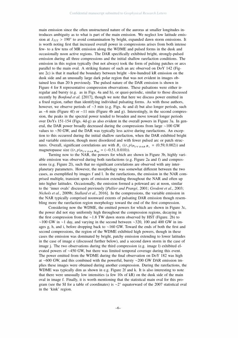
Considering now the auroral morphology, representative images are shown in Fig-ure 2, corresponding to the times labeled at the top of Figure 1. The powers from regionsdelimited by the yellow lines in Figure 2 are shown in Figure 3. These comprise two ac-tive regions observed poleward of the main emission, the well-defined portion of the mainemission over λ I I I > 170◦, and the equatorward region over λ I I I < 190◦. Though theregions are fixed in λ I I I , the well-defined main emission (WDME) region is typically ob-served by HST near dawn, the equatorward region near dusk, while the two poleward re-gions are in the dusk and noon sectors, hence termed here ‘dusk active region’ (DAR) and‘noon active region’ (NAR) respectively. We consider only the well-defined region of the

–4–


1

2

5

10

� ��

/�

a bc d e f g h i j k

1

2

3

�⟂

/�

−900

90180

�(��)

400450500550

� �/��

�−�

10−2

10−1

100

� �/��

6080

100120140

� ��/

�

1374386.414.7

1394236.45.4

1414086.40.2

1433936.44.0

1453786.413.4

1473636.419.4

1493486.315.9

1513336.36.7

1533186.30.7

1553036.33.6

1572876.312.9

1592726.319.7

UT (DoY) / �LT (h)∘�

0

1

2

3

��/�

�(a)

l

(b)

(c)

(d)

Magnetosphere

(e)

(f)

1731586.219.3

1751406.210.9

1771226.23.9

1791036.25.4

181846.214.7

183636.2

24.4

(g)

Figure 1. Plot showing auroral powers and interplanetary data versus UT at the ionosphere. We show (a)

median and range of total UV powers Puv in TW observed by HST in each orbit (black crosses with error

bars) along with powers observed by Hisaki (gray points); (b) B⊥ in nT; (c) IMF clock angle θc in degrees

along with horizontal dotted lines at 0 and ±90◦; (d) vsw in km s−1; (e) psw in nPa; (f) Rmp in RJ; and finally

(g) ΦLL in MV. Vertical dotted lines indicate the times of the HST observations. Also shown by the vertical

dashed and dot-dashed lines are times of an observed eruption on Io and sodium nebula enhancement, re-

spectively. The colors indicate different interplanetary conditions as discussed in the text, and the gray box

indicates where Juno left the solar wind. The letters at the top correspond to the times of the images shown in

Figure 2.

–5–


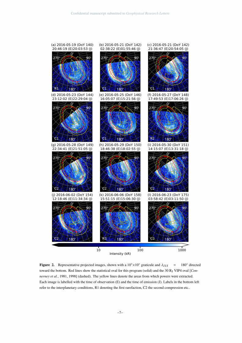
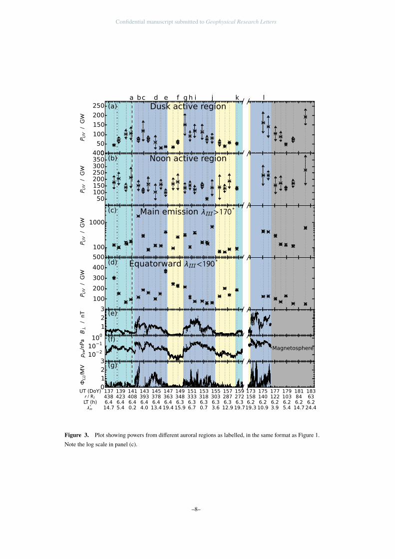
main emission since the often unstructured nature of the auroras at smaller longitudes in-troduces ambiguity as to what is part of the main emission. We neglect low latitude emis-sion at λ I I I > 190◦ to avoid contamination by bright, expanded dawn storm emissions. Itis worth noting first that increased overall power in compressions arises from both intensefew- to a few tens of MR emission along the WDME and pulsed forms in the dusk andoccasionally noon active regions. The DAR specifically exhibited bright, strongly-pulsedemission during all three compressions and the initial shallow rarefaction conditions. Theemission in this region typically (but not always) took the form of pulsing patches or arcsparallel to the main oval. A striking feature of such an arc observed on DoY 142 (Fig-ure 2c) is that it marked the boundary between bright ∼few-hundred kR emission on thedusk side and an unusually large dark polar region that was not evident in images ob-tained less than 20 h previously. The pulsed nature of the DAR emission is shown inFigure 4 for 8 representative compression observations. These pulsations were either ir-regular and bursty (e.g. as in Figs. 4a and h), or quasi-periodic, similar to those discussedrecently by Bonfond et al. [2017], though we note that here we discuss power emitted ina fixed region, rather than identifying individual pulsating forms. As with those authors,however, we observe periods of ∼3 min (e.g. Figs. 4c and d) but also longer periods, suchas ∼6 min (Figure 4f) or ∼11 min (Figure 4b and g). Interestingly, in the second compres-sion, the peaks in the spectral power tended to broaden and move toward longer periodsover DoYs 151-154 (Figs. 4d-g) as also evident in the overall powers in Figure 3a. In gen-eral, the DAR power broadly decreased during the compressions from large ∼100 GWvalues to ∼50 GW, and the DAR was typically less active during rarefactions. An excep-tion to this occurred during the initial shallow rarefaction, when the DAR exhibited brightand variable emission, though more disordered and with fewer pulsed arc or patch struc-tures. Overall, significant correlations are with B⊥ ((r, p)PUV DAR B⊥ = (0.59, 0.002)) andmagnetopause size ((r, p)PUV DAR Rmp = (−0.51, 0.010)).

Turning now to the NAR, the powers for which are shown in Figure 3b, highly vari-able emission was observed during both rarefactions (e.g. Figure 2a and f) and compres-sions (e.g. Figure 2l), such that no significant correlations are observed with any inter-planetary parameters. However, the morphology was somewhat different between the twocases, as exemplified by images f and l. In the rarefactions, the emission in the NAR com-prised multiple, transient spots of emission extending throughout the NAR and often upinto higher latitudes. Occasionally, the emission formed a poleward arc at noon, similarto the ‘inner ovals’ discussed previously [Pallier and Prangé, 2001; Grodent et al., 2003;Nichols et al., 2009b; Stallard et al., 2016]. In the compressions, the variable emission inthe NAR typically comprised noonward extents of pulsating DAR emission though resem-bling more the rarefaction region morphology toward the end of the first compression.

Considering now the WDME, the emitted powers for which are shown in Figure 3c,the power did not stay uniformly high throughout the compression regions, decaying inthe first compression from the ∼1.8 TW dawn storm observed by HST (Figure. 2b) to∼100 GW in ∼1 day, and varying in the second between ∼320, 100 and 400 GW in im-ages g, h, and i, before dropping back to ∼160 GW. Toward the ends of both the first andsecond compressions, the region of the WDME exhibited high powers, though in thesecases the emission was dominated by bright, patchy emission extending to lower latitudesin the case of image e (discussed further below), and a second dawn storm in the case ofimage j. The two observations during the third compression (e.g. image l) exhibited el-evated powers of ∼450 GW, but there was limited temporal coverage during this event.The power emitted from the WDME during the final observation on DoY 182 was highat ∼600 GW, and this combined with the powerful, bursty ∼200 GW DAR emission im-plies these images were obtained during another compression. During the rarefactions, theWDME was typically dim as shown in e.g. Figure 2f and k. It is also interesting to notethat there were unusually low intensities (a few 10s of kR) on the dusk side of the mainoval in image f. Finally, it is worth mentioning that the statistical main oval for this pro-gram (see the SI for a table of coordinates) is ∼2◦ equatorward of the 2007 statistical ovalin the ‘kink’ region.

–6–


��∘

��∘ ��∘�∘

(a) 2016-05-19 (DoY 140)20:46:19 (E) 20:03:53 (J)

R1 ��∘

��∘ ��∘�∘

(b) 2016-05-21 (DoY 142)02:38:22 (E) 01:55:46 (J)

C1 ��∘

��∘ ��∘�∘

(c) 2016-05-21 (DoY 142)21:36:47 (E) 20:54:05 (J)

C1

��∘

��∘ ��∘�∘

(d) 2016-05-23 (DoY 144)23:12:02 (E) 22:29:04 (J)

C1 ��∘

��∘ ��∘�∘

(e) 2016-05-25 (DoY 146)16:05:07 (E) 15:21:56 (J)

C1 ��∘

��∘ ��∘�∘

(f) 2016-05-27 (DoY 148)17:49:53 (E) 17:06:26 (J)

R2

��∘

��∘ ��∘�∘

(g) 2016-05-28 (DoY 149)22:34:41 (E) 21:51:05 (J)

C2 ��∘

��∘ ��∘�∘

(h) 2016-05-29 (DoY 150)18:46:38 (E) 18:02:55 (J)

C2 ��∘

��∘ ��∘�∘

(i) 2016-05-30 (DoY 151)14:15:07 (E) 13:31:18 (J)

C2

��∘

��∘ ��∘�∘

(j) 2016-06-02 (DoY 154)12:18:46 (E) 11:34:34 (J)

C2 ��∘

��∘ ��∘�∘

(k) 2016-06-06 (DoY 158)15:51:15 (E) 15:06:30 (J)

R3 ��∘

��∘ ��∘�∘

(l) 2016-06-23 (DoY 175)03:58:42 (E) 03:11:50 (J)

C3

10 100 1000Intensity (kR)

Figure 2. Representative projected images, shown with a 10◦×10◦ graticule and λ I I I = 180◦ directed

toward the bottom. Red lines show the statistical oval for this program (solid) and the 30 RJ VIP4 oval [Con-

nerney et al., 1981, 1998] (dashed). The yellow lines denote the areas from which powers were extracted.

Each image is labelled with the time of observation (E) and the time of emission (J). Labels in the bottom left

refer to the interplanetary conditions, R1 denoting the first rarefaction, C2 the second compression etc..

–7–


0

50

100

150

200

250

� ��/��

Dusk active region(a)a bc d e f g h i j k

50100150200250300350400

� ��/��

Noon active region(b)

100

1000

� ��/��

Main emission ��>�� ∘(c)

100

200

300

400

500

� ��/��

Equatorward ��<�� ∘(d)

123

�⟂/� (e)

10−210−1100

� /�� (f)

1374386.414.7

1394236.45.4

1414086.40.2

1433936.44.0

1453786.413.4

1473636.419.4

1493486.315.9

1513336.36.7

1533186.30.7

1553036.33.6

1572876.312.9

1592726.319.7

UT (DoY)� / �LT (h)∘�

0123

��/�

� (g)

l

Magnetosphere

1731586.219.3

1751406.210.9

1771226.23.9

1791036.25.4

181846.214.7

183636.2

24.4

Figure 3. Plot showing powers from different auroral regions as labelled, in the same format as Figure 1.

Note the log scale in panel (c).

–8–


100200300400500

� ��

/��

c(a) (i) 2016-05-21 (142) 20:40:25

100200300400500

�()

/��

� (a) (ii)

100200300400500

� ��

/��

g(b) (i) 2016-05-28 (149) 21:12:35

200400600800

10001200

�()

/��

� (b) (ii)

100200300400500

� ��

/��

h(c) (i) 2016-05-29 (150) 17:51:35

50100150200250300

�()

/��

� (c) (ii)

100200300400500

� ��

/��

i(d) (i) 2016-05-30 (151) 12:56:08

50100150200250300

�()

/��

� (d) (ii)

100200300400500

� ��

/��

-(e) (i) 2016-05-31 (152) 19:08:16

50100150200250300

�()

/��

� (e) (ii)

100200300400500

� ��

/��

-(f) (i) 2016-06-01 (153) 14:22:13

50100150200250300

�()

/��

� (f) (ii)

100200300400500

� ��

/��

-(g) (i) 2016-06-02 (154) 10:52:34

50100150200250300

�()

/��

� (g) (ii)

0 5 10 15 20 25 30 35 40 45� / ��

100200300400500

� ��

/��

l(h) (i) 2016-06-23 (175) 02:54:50

0 2 4 6 8 10 12 14 / ��

100200300400500

�()

/��

� (h) (ii)

Figure 4. Plot showing (left) time series of DAR powers obtained during selected orbits, and (right) power

spectra S(τ) of the same, computed using fast Fourier transforms. Start times of the observations corrected

for one-way light time are given, along with the corresponding image in Figure 2 if applicable. Times t and

periods τ are both in units of minutes. Also shown are the 95% and 99% significance levels against the null

hypothesis of white noise (gray dashed and dot-dashed lines, respectively).

–9–


We now consider the low longitude equatorward (LLEQ) emission, the powers forwhich are shown in Figure 3d. This region exhibited emission that varied significantlyover the program, with values of ∼50-350 GW, peaking on DoY 146. The emission wasinitially principally located in the ‘kink’ region (Figure 2c), then taking the form of a sec-ondary arc (Figure 2d), and the high powers on DoYs 146-149 corresponded to patchyemission of varying intensity, in some cases overlapping and extending down from themain emission, as discussed previously by Radioti et al. [2009]; Nichols et al. [2009a]; Du-

mont et al. [2015] and Gray et al. [2016]. Superficially, the equatorward powers seem tobe enhanced in rarefaction regions though, with no significant correlations with any inter-planetary parameter, this is not a robust result.

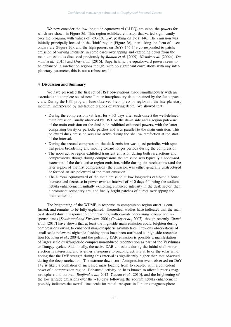
4 Discussion and Summary

We have presented the first set of HST observations made simultaneously with anextended and complete set of near-Jupiter interplanetary data, obtained by the Juno space-craft. During the HST program Juno observed 3 compression regions in the interplanetarymedium, interspersed by rarefaction regions of varying depth. We showed that:

• During the compressions (at least for ∼1-3 days after each onset) the well-definedmain emission usually observed by HST on the dawn side and a region polewardof the main emission on the dusk side exhibited enhanced powers, with the lattercomprising bursty or periodic patches and arcs parallel to the main emission. Thispoleward dusk emission was also active during the shallow rarefaction at the startof the interval.

• During the second compression, the dusk emission was quasi-periodic, with spec-tral peaks broadening and moving toward longer periods during the compression.

• The noon active region exhibited transient emission during both rarefactions andcompressions, though during compressions the emission was typically a noonwardextension of the dusk active region emission, while during the rarefactions (and thelater region of the first compression) the emission was either generally unstructuredor formed an arc poleward of the main emission.

• The auroras equatorward of the main emission at low longitudes exhibited a broadincrease and decrease in power over an interval of ∼10 days following the sodiumnebula enhancement, initially exhibiting enhanced intensity in the dusk sector, thena prominent secondary arc, and finally bright patches of aurora overlapping themain emission.

The brightening of the WDME in response to compression region onset is con-firmed, and remains to be fully explained. Theoretical studies have indicated that the mainoval should dim in response to compressions, with caveats concerning ionospheric re-sponse times [Southwood and Kivelson, 2001; Cowley et al., 2007], though recently Chané

et al. [2017] have shown that at least the nightside main emission could brighten duringcompressions owing to enhanced magnetospheric asymmetries. Previous observations ofsmall-scale poleward nightside flashing spots have been attributed to nightside reconnec-tion [Grodent et al., 2004], and the pulsating DAR emission is possibly a manifestationof larger scale dusk/nightside compression-induced reconnection as part of the Vasyliunasor Dungey cycles. Additionally, the active DAR emissions during the initial shallow rar-efaction is interesting and is either a response to ongoing activity at Io or the solar wind,noting that the IMF strength during this interval is significantly higher than that observedduring the deep rarefaction. The extreme dawn storm/compression event observed on DoY142 is likely a conflation of increased mass loading from Io coupled with a coincidentonset of a compression region. Enhanced activity on Io is known to affect Jupiter’s mag-netosphere and auroras [Bonfond et al., 2012; Yoneda et al., 2010], and the brightening ofthe low latitude emissions over the ∼10 days following the sodium nebula enhancementpossibly indicates the overall time scale for radial transport in Jupiter’s magnetosphere

–10–


[Louarn et al., 2014; Gray et al., 2016], though it is also consistent with the conclusionsof Mauk et al. [1999] that clustered energetic particle injections are associated with so-lar wind rarefactions. The lack of a correlation between the NAR powers and any inter-planetary parameters (e.g. vsw or B⊥) was surprising, but as noted above the morphologywas typically distinct between compressions and rarefactions. It seems that the NAR re-gion is neither driven simply by Kelvin-Helmholtz instability at the magnetopause, norreconnection according to the coupling function used here. Overall, these results evince adependance of Jupiter’s auroras on the interplanetary medium, which thus acts to triggermagnetospheric activity, but that this more complex than previously thought.

Acknowledgments

This work is based on observations made with the NASA/ESA Hubble Space Telescope(program GO 14105), obtained at STScI, which is operated by AURA, Inc. for NASA.Work at Leicester was supported by STFC Fellowship (ST/I004084/1) and STFC GrantST/K001000/1. SVB was supported by STFC Grant ST/M005534/1. JTC was supportedby grant HST-GO-14105.002-A from STScI to Boston University. Data are available at theMAST Archive (HST), and Wilson and al [2017] and McComas et al. [2017] (Juno).

References

Badman, S. V., and S. W. H. Cowley (2007), Significance of Dungey-cycle flows inJupiter’s and Saturn’s magnetospheres, and their identification on closed equatorial fieldlines, Ann. Geophysicae, 25(4), 941–951.

Badman, S. V., B. Bonfond, M. Fujimoto, R. L. Gray, Y. Kasaba, S. Kasahara, T. Kimura,H. Melin, J. D. Nichols, A. J. Steffl, C. Tao, F. Tsuchiya, A. Yamazaki, M. Yoneda,I. Yoshikawa, and K. Yoshioka (2016), Weakening of Jupiter’s main auroral emissionduring January 2014, Geophys. Res. Lett., 43(3), 988–997, doi:10.1002/2015GL067366.

Baron, R. L., T. Owen, J. E. P. Connerney, T. Satoh, and J. Harrington (1996), Solar windcontrol of Jupiter’s H+3 Auroras, Icarus, 120(2), 437–442, doi:10.1006/icar.1996.0063.

Bonfond, B., D. Grodent, J.-C. Gérard, T. S. Stallard, J. T. Clarke, M. Yoneda, A. Radi-oti, and J. Gustin (2012), Auroral evidence of Io’s control over the magnetosphere ofJupiter, Geophys. Res. Lett., 39(1), L01,105–n/a, doi:10.1029/2011GL050253.

Bonfond, B., D. Grodent, S. V. Badman, J.-C. Gérard, and A. Radioti (2017), Dynamicsof the flares in the active polar region of Jupiter , Geophys. Res. Lett., in press.

Brice, N. M., and G. A. Ioannidis (1970), The magnetospheres of Jupiter and Earth,Icarus, 13(2), 173–183, doi:10.1016/0019-1035(70)90048-5.

Chané, E., J. Saur, R. Keppens, and S. Poedts (2017), How is the Jovian Main AuroralEmission Affected by the Solar Wind?, J. Geophys. Res., in press.

Clarke, J. T., D. Grodent, S. W. H. Cowley, E. J. Bunce, P. M. Zarka, J. E. P. Connerney,and T. Satoh (2004), Jupiter’s aurora, in Jupiter.~The Planet, Satellites and Magneto-

sphere, edited by F. Bagenal and W. B. McKinnon, pp. 639–670, Cambridge. Univ.Press, Cambridge, UK.

Clarke, J. T., J. D. Nichols, J.-C. Gérard, D. Grodent, K. C. Hansen, W. S. Kurth, G. R.Gladstone, J. Duval, S. Wannawichian, E. J. Bunce, S. W. H. Cowley, F. J. Crary,M. K. Dougherty, L. Lamy, D. G. Mitchell, W. R. Pryor, K. D. Retherford, T. S.Stallard, B. Zieger, P. M. Zarka, and B. Cecconi (2009), Response of Jupiter’s andSaturn’s auroral activity to the solar wind, J. Geophys. Res., 114(A), A05,210, doi:10.1029/2008JA013694.

Connerney, J. E. P., J. B. Bjarno, T. Denver, M. Benn, J. Espley, J. L. Jorgensen, P. S. Jor-gensen, P. Lawton, A. Malinnikova, J. M. Merayo, S. Murphy, J. Odom, R. Oliversen,R. Schurr, D. Sheppard, and E. J. Smith (), The Juno Magnetic Field Investigation,Space Sci. Rev., doi:10.1007/s11214-017-0334-z.

Connerney, J. E. P., M. H. Acuña, and N. F. Ness (1981), Modeling the Jovian currentsheet and inner magnetosphere, J. Geophys. Res., 86, 8370–8384.

–11–


Connerney, J. E. P., M. H. Acuña, N. F. Ness, and T. Satoh (1998), New models ofJupiter’s magnetic field constrained by the Io flux tube footprint, J. Geophys. Res.,103(A6), 11,929–11,940, doi:10.1029/97JA03726.

Cowley, S. W. H., J. D. Nichols, and D. J. Andrews (2007), Modulation of Jupiter’splasma flow, polar currents, and auroral precipitation by solar wind-induced compres-sions and expansions of the magnetosphere: a simple theoretical model, Ann. Geophysi-

cae, 25, 1433–1463.Cowley, S. W. H., S. V. Badman, S. M. Imber, and S. E. Milan (2008), Comment

on “Jupiter: A fundamentally different magnetospheric interaction with the solarwind” by D. J. McComas and F. Bagenal, Geophys. Res. Lett., 35(10), L10,101, doi:10.1029/2007GL032645.

Delamere, P. A., and F. Bagenal (2010), Solar wind interaction with Jupiter’s magneto-sphere, J. Geophys. Res., 115(A), A10,201, doi:10.1029/2010JA015347.

Dumont, M., D. Grodent, A. Radioti, B. Bonfond, and J.-C. Gérard (2015), Jupiter’s equa-torward auroral features: Possible signatures of magnetospheric injections, pp. 1–10,doi:10.1002/(ISSN)2169-9402.

Dunn, W. R., G. Branduardi-Raymont, R. F. Elsner, M. F. Vogt, L. Lamy, P. G. Ford,A. J. Coates, G. R. Gladstone, C. M. Jackman, J. D. Nichols, I. J. Rae, A. Varsani,T. Kimura, K. C. Hansen, and J. M. Jasinski (2016), The impact of an ICME on the Jo-vian X-ray aurora, Journal of Geophysical Research: Space Physics, 121(3), 2274–2307,doi:10.1002/2015JA021888.

Gray, R. L., S. V. Badman, and B. Bonfond (2016), Auroral evidence of radial transport atJupiter during January 2014, J. Geophys. Res., 121, doi:10.1002/(ISSN)2169-9402.

Grodent, D., J. T. Clarke, J. H. Waite Jr, S. W. H. Cowley, J.-C. Gérard, and J. Kim(2003), Jupiter’s polar auroral emissions, J. Geophys. Res., 108(A10), 1366, doi:10.1029/2003JA010017.

Grodent, D., J.-C. Gérard, J. T. Clarke, G. R. Gladstone, and J. H. Waite Jr (2004), A pos-sible auroral signature of a magnetotail reconnection process on Jupiter, J. Geophys.

Res., 109(A18), 5201, doi:10.1029/2003JA010341.Gustin, J., B. Bonfond, D. Grodent, and J.-C. Gérard (2012), Conversion from HST ACS

and STIS auroral counts into brightness, precipitated power, and radiated power for H2

giant planets, J. Geophys. Res., 117(A7), A07,316, doi:10.1029/2012JA017607.Joy, S. P., M. G. Kivelson, R. J. Walker, K. K. Khurana, C. T. Russell, and T. Ogino

(2002), Probabilistic models of the Jovian magnetopause and bow shock locations, J.

Geophys. Res., 107(A10), SMP 17–1–SMP 17–17, doi:10.1029/2001JA009146.Khurana, K. K., M. G. Kivelson, V. M. Vasyliunas, N. Krupp, J. Woch, A. Lagg, B. H.

Mauk, and W. S. Kurth (2004), The configuration of Jupiter’s magnetosphere, inJupiter.~The Planet, Satellites and Magnetosphere, edited by F. Bagenal, T. E. Dowling,and W. B. McKinnon, pp. 593–616, Cambridge. Univ. Press.

Kimura, T., and et al. (2017), Auroral explosion at Jupiter observed by the Hisaki satelliteand Hubble SpaceâĂĺ , Geophys. Res. Lett., submitted.

Kimura, T., R. P. Kraft, R. F. Elsner, G. Branduardi-Raymont, G. R. Gladstone, C. Tao,K. Yoshioka, G. Murakami, A. Yamazaki, F. Tsuchiya, M. F. Vogt, A. Masters,H. Hasegawa, S. V. Badman, E. Roediger, Y. Ezoe, W. R. Dunn, I. Yoshikawa, M. Fu-jimoto, and S. S. Murray (2016), Jupiter's X-ray and EUV auroras monitored byChandra, XMM-Newton, and Hisaki satellite, Journal of Geophysical Research: Space

Physics, 121(3), 2308–2320, doi:10.1002/2015JA021893.Kita, H., T. Kimura, C. Tao, F. Tsuchiya, H. Misawa, T. Sakanoi, Y. Kasaba, G. Mu-

rakami, K. Yoshioka, A. Yamazaki, I. Yoshikawa, and M. Fujimoto (2016), Characteris-tics of solar wind control on Jovian UV auroral activity deciphered by long-term HisakiEXCEED observations: Evidence of preconditioning of the magnetosphere?, Geophys.

Res. Lett., 43(1), 6790–6798, doi:10.1002/2016GL069481.Louarn, P., C. P. Paranicas, and W. S. Kurth (2014), Global magnetodisk disturbances and

energetic particle injections at Jupiter, Journal of Geophysical Research: Space Physics,

–12–


119(6), 4495–4511, doi:10.1002/2014JA019846.Mauk, B. H., D. J. Williams, R. W. McEntire, K. K. Khurana, and J. G. Roederer (1999),

Storm-like dynamics of Jupiter’s inner and middle magnetosphere, J. Geophys. Res.,104(A10), 22,759–22,778, doi:10.1029/1999JA900097.

McComas, D. J., and F. Bagenal (2007), Jupiter: A fundamentally different magneto-spheric interaction with the solar wind, Geophys. Res. Lett., 34(20), L20,106, doi:10.1029/2007GL031078.

McComas, D. J., N. Alexander, F. Allegrini, F. Bagenal, C. Beebe, G. Clark, F. J.Crary, M. I. Desai, A. De Los Santos, D. Demkee, J. Dickinson, D. Everett, T. Fin-ley, A. Gribanova, R. Hill, J. Johnson, C. Kofoed, C. Loeffler, P. Louarn, M. Maple,W. Mills, C. Pollock, M. Reno, B. Rodriguez, J. Rouzaud, D. Santos-Costa, P. Valek,S. Weidner, P. Wilson, R. J. Wilson, and D. White (2013), The Jovian Auroral Dis-tributions Experiment (JADE) on the Juno Mission to Jupiter, Space Sci. Rev., doi:10.1007/s11214-013-9990-9.

McComas, D. J., J. R. Szalay, F. Allegrini, F. Bagenal, S. J. Bolton, J. E. P. Conner-ney, R. W. Ebert, G. R. Gladstone, W. S. Kurth, S. M. Levin, P. Louarn, B. H. Mauk,C. Pollock, M. Reno, M. F. Thomsen, P. Valek, S. Weidner, and R. J. Wilson (2017),Plasma environment at the dawn flank of Jupiter’s magnetosphere: Juno arrives atJupiter, Geophys. Res. Lett., submitted.

Nichols, J. D., S. W. H. Cowley, and D. J. McComas (2006), Magnetopause reconnec-tion rate estimates for Jupiter’s magnetosphere based on interplanetary measurements at∼5AU, Ann. Geophysicae, 24, 393–406.

Nichols, J. D., E. J. Bunce, J. T. Clarke, S. W. H. Cowley, J.-C. Gérard, D. Grodent, andW. R. Pryor (2007), Response of Jupiter’s UV auroras to interplanetary conditions asobserved by the Hubble Space Telescope during the Cassini flyby campaign, J. Geo-

phys. Res., 112(A11), A02,203, doi:10.1029/2006JA012005.Nichols, J. D., J. T. Clarke, J.-C. Gérard, D. Grodent, and K. C. Hansen (2009a), Varia-

tion of different components of Jupiter’s auroral emission, J. Geophys. Res., 114(A6),A06,210, doi:10.1029/2009JA014051.

Nichols, J. D., J. T. Clarke, J.-C. Gérard, and D. Grodent (2009b), Observationsof Jovian polar auroral filaments, Geophys. Res. Lett., 36(8), L08,101, doi:10.1029/2009GL037578.

Pallier, L., and R. Prangé (2001), More about the structure of the high latitude Jovian au-rorae, Planet. Space Sci., 49(10-11), 1159–1173, doi:10.1016/s0032-0633(01)00023-x.

Pryor, W. R., A. I. F. Stewart, L. W. Esposito, W. E. McClintock, J. E. Colwell, A. J. Jou-choux, A. J. Steffl, D. E. Shemansky, J. M. Ajello, R. A. West, C. J. Hansen, B. T. Tsu-rutani, W. S. Kurth, G. B. Hospodarsky, D. A. Gurnett, K. C. Hansen, J. H. Waite Jr,F. J. Crary, D. T. Young, N. Krupp, J. T. Clarke, D. Grodent, and M. K. Dougherty(2005), Cassini UVIS observations of Jupiter’s auroral variability, Icarus, 178(2), 312–326, doi:10.1016/j.icarus.2005.05.021.

Radioti, A., A. T. Tomas, D. Grodent, J.-C. Gérard, J. Gustin, B. Bonfond, N. Krupp,J. Woch, and J. D. Menietti (2009), Equatorward diffuse auroral emissions at Jupiter:Simultaneous HST and Galileo observations, Geophys. Res. Lett., 36(7), n/a–n/a, doi:10.1029/2009GL037857.

Southwood, D. J., and M. G. Kivelson (2001), A new perspective concerning the influenceof the solar wind on the Jovian magnetosphere, J. Geophys. Res., 106(A4), 6123–6130,doi:10.1029/2000JA000236.

Stallard, T. S., J. T. Clarke, H. Melin, S. Miller, J. D. Nichols, J. O’Donoghue, R. E.Johnson, J. E. P. Connerney, T. Satoh, and M. Perry (2016), Stability within Jupiter’spolar auroral ’Swirl region’ over moderate timescales, Icarus, 268, 145–155, doi:10.1016/j.icarus.2015.12.044.

Tao, C., T. Kimura, S. V. Badman, N. Andre, F. Tsuchiya, G. Murakami, K. Yoshioka,I. Yoshikawa, A. Yamazaki, and M. Fujimoto (2016), Variation of Jupiter’s aurora ob-served by Hisaki/EXCEED: 2. Estimations of auroral parameters and magnetospheric

–13–


dynamics, Journal of Geophysical Research: Space Physics, 121(5), 4055–4071, doi:10.1002/2015JA021272.

Wilson, R. J., and al (2017), Solar Wind Properties During Juno’s approach to Jupiter: 1.Data Analysis and Resulting Plasma Properties Utilizing a 1D Forward model, Geophys.

Res. Lett., submitted.Yoneda, M., H. Nozawa, H. Misawa, M. Kagitani, and S. Okano (2010), Jupiter’s

magnetospheric change by Io’s volcanoes, Geophys. Res. Lett., 37(11), n/a–n/a, doi:10.1029/2010GL043656.

–14–

Documents

Response of Jupiter’s auroras to conditions in the