Resources and Energy Quarterly - March Quarter 2012 · Web viewIn the review section of Resources and Energy Quarterly there is a review of the on-going euro crisis; a review of an

Resourcesand Energy

QuarterlyJune quarter 2012

BREE 2012, Resources and Energy Quarterly, June Quarter 2012, BREE, Canberra, June 2012.

© Commonwealth of Australia 2012

This work is copyright, the copyright being owned by the Commonwealth of Australia. The Commonwealth of Australia has, however, decided that, consistent with the need for free and open re-use and adaptation, public sector information should be licensed by agencies under the Creative Commons BY standard as the default position. The material in this publication is available for use according to the Creative Commons BY licensing protocol whereby when a work is copied or redistributed, the Commonwealth of Australia (and any other nominated parties) must be credited and the source linked to by the user. It is recommended that users wishing to make copies from BREE publications contact the Chief Economist, Bureau of Resources and Energy Economics (BREE). This is especially important where a publication contains material in respect of which the copyright is held by a party other than the Commonwealth of Australia as the Creative Commons licence may not be acceptable to those copyright owners.

The Australian Government acting through BREE has exercised due care and skill in the preparation and compilation of the information and data set out in this publication. Notwithstanding, BREE, its employees and advisers disclaim all liability, including liability for negligence, for any loss, damage, injury, expense or cost incurred by any person as a result of accessing, using or relying upon any of the information or data set out in this publication to the maximum extent permitted by law.

ISSN 1839-499X (Print)

ISSN 1839-5007 (Online)

Vol. 1, no. 4

From 1 July 2011, responsibility for resources and energy data and research was transferred from ABARES to the Bureau of Resources and Energy Economics (BREE).

Postal address:

Bureau of Resources and Energy Economics

GPO Box 1564

Canberra ACT 2601 Australia

Phone: +61 2 6276 1000

Email: [email protected]

Web: www.bree.gov.au

mailto:[email protected]

ForewordResources and Energy Quarterly is an important publication of the Bureau of Resources and Energy Economics (BREE). This issue provides an overview of the global macroeconomic situation; the most up-to-date global production, exports and values of major resources energy commodities and forecasts for 2011–2012 and 2012–13; reviews of key topics and issues of relevance to the sector; and detailed statistical tables on world production, consumption, stocks and trade in key commodities. The statistical tables in this and subsequent issues of Resources and Energy Quarterly incorporate what were previously published every quarter in BREE’s Resources and Energy Statistics.

In the review section of Resources and Energy Quarterly there is a review of the on-going euro crisis; a review of an analysis of end use energy intensity of major household appliances; and an overview of the Australian coal industry.

BREE’s latest forecast for the value of Australian exports of resources and energy for 2011–12 is about A$193 billion or about an 8 per cent increase from 2010–11. The forecast for 2012–13 is for the export value of resources and energy to increase by about 8 per cent to around A$209 billion. Much of this rise in export values is because of large projected increases in the volume of bulk commodity exports.

Quentin Grafton

Executive Director/Chief Economist

Bureau of Resources and Energy Economics

3

ContentsForeword..................................................................................................................................3

Contents...................................................................................................................................4

Acronyms and abbreviations....................................................................................................5

Macroeconomic outlook update and energy and minerals overview.......................................6

Energy outlook........................................................................................................................15

Oil.......................................................................................................................................15

Gas......................................................................................................................................18

Thermal coal.......................................................................................................................19

Resources outlook...................................................................................................................22

Steel and steel-making raw materials.................................................................................22

Gold....................................................................................................................................29

Metals overview.................................................................................................................32

Copper................................................................................................................................34

Aluminium..........................................................................................................................38

Nickel..................................................................................................................................42

Zinc.....................................................................................................................................46

Reviews...................................................................................................................................50

PIIGS, a Trojan horse and an optimal currency area...........................................................51

Energy intensity analysis of household appliances in Australia..........................................57

A short background of the Australian coal industry............................................................71

Statistical tables......................................................................................................................77

4

Acronyms and abbreviationsABARES Australian Bureau of Agricultural and Resource Economics and Science

ABS Australian Bureau of Statistics

BREE Bureau of Resources and Energy Economics

FOB free on board

GDP gross domestic product

IEA International Energy Agency

IMF International Monetary Fund

LME London Metal Exchange

LNG liquefied natural gas

mb/d millions of barrels per day

MBtu million British thermal units

Mt million tonnes

OECD Organisation for Economic Co-operation and Development

OPEC Organisation of the Petroleum Exporting Countries

PPP purchasing-power parity

RBA Reserve Bank of Australia

TWI trade-weighted index

UNCTAD United Nations Conference on Trade and Development

WTI West Texas Intermediate

5

Macroeconomic outlook update and energy and minerals overviewNhu Che, Quentin Grafton and Pam Pham

Growth continues, but remains fragile with elevated downside risks

The global economy is projected to grow slowly in 2012 relative to 2011, and will remain fragile and subject to substantial downside risks. The updated World Economic Outlook (WEO) released by the International Monetary Fund (IMF) in April 2012 projects improved economic activity in the US during the second half of 2012, and a more expansionary policies in the euro area in response to the deepening economic crisis in the euro zone. In general, weak recovery is expected in key advanced economies, but economic activity is expected to remain robust in most emerging and developing economies. The ongoing political and economic crisis in Greece, and recent data that indicate a lower than expected rate of growth in China, are key concerns for the short-term outlook.

Global growth is projected to drop from about 3.7 per cent in 2011 to about 3.25 per cent in 2012 due to a slowdown caused by deteriorating sovereign and banking sector developments in the euro zone attributable to the current Greek economic crisis. The IMF (the April WEO) predicts a gradual renewal of economic activity and a return to about 4 per cent global economic growth in 2013.

Economic conditions in Europe remain problematic. Some progress has been made in addressing fiscal imbalances and implementing structural reforms, but much work remains to be done. The IMF (the April WEO) records that the balance of risks to Europe’s near-term growth prospects remains on the downside. Despite the progress in strengthening crisis management in recent months, a renewed escalation of the euro crisis and the Greek economic crisis remains a possibility as long as the underlying issues are not resolved (see Review article on the euro crisis). The euro zone is still projected to drop into a mild recession in 2012 as a result of the Greek sovereign debt crisis and a general loss of confidence, the effects of bank deleveraging on the real economy, and the impact of fiscal consolidation in response to market pressures. Added to this, lower than expected economic growth in China may have a negative impact on a number of advanced economies, including Australia.

Real GDP growth in the emerging and developing economies is projected to slow from 6.4 per cent in 2011 to 6.0 per cent in 2012, but then to reaccelerate to 6.3 per cent in 2013. The euro zone may face a further crisis, recession, and possible contagion. The spill-over from the euro zone crisis could also severely affect the rest of Europe. Other European economies would likely experience further financial volatility, although no major impact on activity is expected unless the euro zone crisis intensifies further. Downside risks may be accelerated if there were to be a disruption in global bond and currency markets that would be exacerbated by high

6

budget deficits and debt in Japan and the US, and could result in rapidly slowing activity in some emerging economies.

In the 17 June Greek election the New Democracy party, under the leadership of Antonis Samaras, won the highest number of votes and it has formed a coalition government. The election outcome has been viewed favourably by market commentators because the New Democracy Party is broadly in favour of the Greek bail-out and maintaining Greece within the euro zone.

Economic growth was robust in most of Asia and Latin America in 2011, but is expected to moderate in 2012 before regaining strength in 2013. Unlike some advanced economies concerned with lagging growth, the immediate concern for some of these emerging economies is their rising inflation.

In Asia, recent data are broadly consistent with the modest slowdown that some authorities in the region have been trying to achieve in order to contain inflationary pressures. India and China, in particular, are trying to reduce the rates of price increases, and their actions have already moderated their previously very high rates of economic growth.

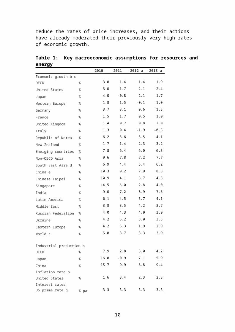
Table 1: Key macroeconomic assumptions for resources and energy2010 2011 2012 a 2013 a

Economic growth b c OECD % 3.0 1.4 1.4 1.9

United States % 3.0 1.7 2.1 2.4

Japan % 4.0 –0.8 2.1 1.7

Western Europe % 1.8 1.5 –0.1 1.0

Germany % 3.7 3.1 0.6 1.5

France % 1.5 1.7 0.5 1.0

United Kingdom % 1.4 0.7 0.8 2.0

Italy % 1.3 0.4 –1.9 –0.3

Republic of Korea % 6.2 3.6 3.5 4.1

New Zealand % 1.7 1.4 2.3 3.2

Emerging countries % 7.8 6.4 6.0 6.3

Non-OECD Asia % 9.6 7.8 7.2 7.7

South East Asia d % 6.9 4.4 5.4 6.2

China e % 10.3 9.2 7.9 8.3

Chinese Taipei % 10.9 4.1 3.7 4.8

Singapore % 14.5 5.0 2.8 4.0

India % 9.0 7.2 6.9 7.3

Latin America % 6.1 4.5 3.7 4.1

Middle East % 3.8 3.5 4.2 3.7

Russian Federation % 4.0 4.3 4.0 3.9

Ukraine % 4.2 5.2 3.0 3.5

Eastern Europe % 4.2 5.3 1.9 2.9

World c % 5.0 3.7 3.3 3.9

7

2010 2011 2012 a 2013 a

Industrial production bOECD % 7.9 2.8 3.0 4.2

Japan % 16.0 –0.9 7.1 5.9

China % 15.7 9.9 8.8 9.4

Inflation rate bUnited States % 1.6 3.4 2.3 2.3

Interest ratesUS prime rate g % pa 3.3 3.3 3.3 3.3

a BREE assumption. b Change from previous period. c Weighted using 2012 purchasing power parity (PPP) valuation of country gross domestic product by the IMF. d Indonesia, Malaysia, the Philippines, Thailand and Vietnam. e Excludes Hong Kong. g Commercial bank lending rates to prime borrowers in the US.Sources: BREE; ABS; IMF; OECD; RBA.

Economic prospects in Australia’s major mining export markets

Non-OECD economies

China’s rapid economic growth provides a substantial impact on the demand for energy and mining products imported from Australia. Although economic growth has moderated since mid-2011, consumption and investment are expected to remain robust. Growth has slowed to a more sustainable pace in China largely as a result of the effect of tighter domestic policies, which have helped to ease inflationary pressures. Chinese economic growth is projected to be around 8 per cent in 2012 and 2013. Commodity imports and consumption of more cyclical commodities—especially base metals, but also crude oil—have increased at a robust pace, in part due to continued solid domestic investment growth.

The Chinese economy continues to record strong growth, although this is projected to moderate in 2012. In part, this expected easing in economic growth is due to domestic economic policies to combat inflation, including the continuing unwinding of the 2008–09 fiscal stimulus, tighter monetary policy, and measures to contain price increases in its property market. Additionally, spill-over from problems in the broader global economy and some high internal risks facing the Chinese economy pose risks to its targeted level of economic growth. Based on purchasing power parity terms (PPP), China’s gross domestic product (GDP) is assumed to grow at 7.9 per cent in 2012. This is 0.3 percentage points lower than that assumed by BREE in March 2012. An annual rate of economic growth of 8.3 per cent is assumed for 2013.

Despite a slight moderation in its economic growth, Chinese domestic demand remains strong. Retail sales continue to expand and passenger vehicle sales are just below their late 2010 peak level. Although there has been relatively weaker export demand, manufacturing investment continues to grow. As a result, over the outlook period China is expected to continue its major role as a growth engine for the world economy.

8

Figure 1: Economic growth in Australia’s major resource and energy export markets

Please refer to page 9 of the Resources and Energy Quarterly – June quarter 2011 PDF version.

The April WEO by the IMF discusses whether China will unexpectedly enter another period of ‘destocking’. The recent increase in cancelled warrants relative to total stocks in London Metal Exchange warehouses, which is a leading indicator of declining metal inventory buffers in the near term, is consistent with an expectation of robust growth in the demand for base metals over the near term in China.

Economic growth in India has moderated due to policies intended to combat rising inflationary pressures. Economic growth is projected to be 6.9 per cent in 2012, 0.1 percentage points lower than assumed by BREE in March 2012. The slowing in growth follows a significant tightening in monetary policy. Given a slight decrease in industrial production over the past quarter, industrial production in 2012 is projected to grow at around 5.9 per cent. This is below its early 2011 peak and 0.1 percentage points lower than expected by BREE in March 2012. In addition to the effect of tighter monetary policy, industrial production has also been affected by problems at a number of coal mines that have disrupted the fuel supply for coal-fired power stations.

Due to robust investment, near-term growth in ASEAN countries (including Indonesia, Malaysia, Philippines, Thailand, and Vietnam) is assumed to be around 5.4 per cent in 2012. This investment should offset a possible slowdown in export momentum.

OECD economies

Economic growth in OECD economies is assumed to be 1.4 per cent in 2012. The annual growth rate in Japan is assumed to be 2.1 per cent, 0.4 percentage points lower than assumed in March 2012 by BREE. The pace of growth in the 17 countries in the euro zone slowed in 2011, and is expected to deteriorate further in 2012. An expected slow-down in growth in the core northern euro zone economies, such as Germany, is likely to make economic conditions in the southern economies more difficult in 2012.

The German economy was the most robust economy in Western Europe in 2011, with strong export-led growth of 3.1 per cent. According to the April WEO projection, growth will slow in terms of industrial production and economic growth in 2012. Nevertheless, in the first quarter of 2012 the German economy actually grew more than expected due to exports to emerging markets which offset waning euro-area demand. With the euro region’s debt crisis ravaging economies from Greece to Spain, German companies have shifted focus to emerging markets. Car makers and their suppliers are benefitting from demand in faster-growing markets such as China, while falling unemployment and rising wages are stimulating spending at home.

9

The US economy improved throughout 2011 and continues to expand at a moderate rate in 2012. US economic activity gained strength through the year, with the quarterly growth rate rising each quarter. Growth in the US was determined primarily by domestic factors in 2011, and is estimated to grow at a rate of 2.1 per cent in 2012 and 2.4 per cent in 2013.

The US unemployment rate has declined in the past year and there are tentative signs of improvement in housing construction activity. Economic growth is expected to be supported by increases in consumption and business investment, with forward-looking indicators of economic activity improving. Assumed very low nominal interest rates over the next two years are expected to provide support to investment. Risks to the outlook include fiscal uncertainty, rapid fiscal consolidation from start of 2013, weakness in the housing market, and a potential financial spill-over from Europe.

The Republic of Korea’s economy is expected to grow at around 3.5 per cent in 2012, 0.9 percentage points lower than assumed in March 2012 by BREE. The Republic of Korea’s economic growth slowed recently due to lower exports caused by Europe’s debt crisis and the region’s economic downturn. Exports contracted 4.7 percent on-year in April, primarily as a result of decreases in shipments to the EU and Japan. The Republic of Korea’s economy, which heavily depends on overseas demand, has begun to show signs of the effects of weaker exports. Output in the mining and manufacturing sectors fell slightly in the first quarter of 2012.

Australia’s economic prospects

Real GDP in Australia, based on a PPP valuation of GDP, is assumed to grow at an annual rate of 2.9 per cent in 2011–12, 0.9 percentage points lower than expected in March 2012 by BREE. The decrease in anticipated economic growth in 2011–12 is primarily a result of lower than expected economic growth in the last quarter of 2011. The Reserve Bank of Australia cites the key factors contributing to lower annual growth are weaker export growth, including a decreasing trend in price within several economic sectors (such as mining); the appreciation of the exchange rate; and lower-than-anticipated growth in the global economy. Additionally, public spending was less than expected, private demand grew roughly as anticipated, dwelling investment was slightly weaker, and business investment slightly stronger.

The Australian economy is assumed to rebound in 2012–13 and grow at around 3.8 cent. The growth in the Australian economy is expected to be supported by mining-related activities, including high levels of mining investment. Significant expansions of iron ore and coal production capacity are underway, and are expected to contribute to solid growth in resource export volumes over the foreseeable future.

Overall, Australian domestic demand continues to grow at a robust pace, although the high level of the exchange rate and rapid growth in mining investment is offset by weak building activity and fiscal consolidation. Export growth is assumed to be at an above-trend pace, due to large volume increases.

10

Table 2: Australia’s key macroeconomic assumptions for resources and energy

2009–10 2010–11 2011–12 a 2012–13 aEconomic growth b c % 2.3 1.8 2.9 3.8Inflation rate b % 2.3 3.1 2.7 2.9Interest rates d % pa 6.0 6.6 7.2 6.7Nominal exchange rates eUS$/A$ US$ 0.88 0.99 1.03 1.01Trade weighted index for A$ g index 69 74 76 76

a BREE assumption. b Change from previous period. c Weighted using 2011 purchasing power parity (PPP) valuation of country gross domestic product by IMF. d Large business weighted average variable rate on credit outstanding. e Average of daily rates. g Base: May 1970 = 100.Sources: BREE; ABS; RBA.

The Australian dollar traded across a wide range during the first half of 2012. In mid-June 2012, the Australian dollar traded around US99c while the trade-weighted index was around 75. In March the Australian dollar traded at US102c and TWI 76. This compares with US104c and TWI 77 in January 2012. The recent fall of the Australian dollar from a peak of US108c and TWI 79 in late February 2012 is a result of interest rate cuts by the Reserve Bank of Australia (RBA) in the second quarter of 2012.

There are several important drivers of the Australian exchange rate over the near term. Factors that would make the Australian dollar relatively weaker include a continuation of the euro zone recession; reduced demand for China’s exports to Europe; improved economic activity in the US; lower economic growth in China; and further interest rate cuts by the RBA in 2012.

Australian resources and energy commodities production and exports

In 2010–11, the gross value added produced from mining activities decreased by 2 per cent to $100.7 billion (in 2011–12 dollars) compared with 2009–10. By contrast, total employment in the mining sector increased by 19 per cent to total 205 300 people. Most of this increase is attributable to employment in the metal ore industry and the coal industry.

The Australian mine production index is forecast to increase by 6 per cent in 2012–13, relative to 2011–12, primarily due to a 7 per cent increase in the output of energy commodities, particularly uranium and black coal. Another contributing factor to this growth will be a forecast of 5 per cent increase in the production of metals and other minerals, underpinned by rising copper and gold production. Projected year-on-year volume increases in terms of Australia’s bulk commodities (iron ore, metallurgical and thermal coal, and LNG) in 2012-13 are expected to be in excess of 10 per cent.

11

Figure 2: Australian mine production index


In 2012–13, the total export earnings for energy and mineral commodities are forecast to increase by 8 per cent to $209.5 billion supported by increases in the export values for both energy and mineral commodities (see Figure 3). Energy commodity export earnings in 2012–13 are anticipated to grow by 7 per cent to $82.3 billion as a result of strong increases in export earnings from thermal coal (up 7 per cent to $18.6 billion), LNG (up 29 per cent to $16.0 billion) and uranium (up 9 per cent to $800 million).

Figure 3: Australian energy and minerals export earnings


Mineral commodity export earnings in 2012–13 are forecast to increase by 10 per cent to $127.1 billion as a result of increases in the export values of alumina (up 30 per cent to $7.1 billion), gold (up 27 per cent to $19.7 billion), iron ore (up 7 per cent to $67 billion) and copper (up 7 per cent to $9 billion). Partially offsetting the increased export earnings for mineral commodities will be lower forecast export earnings for aluminium (down 12 per cent to $3.4 billion) and metallurgical coal (down 2 per cent to $29.7 billion).

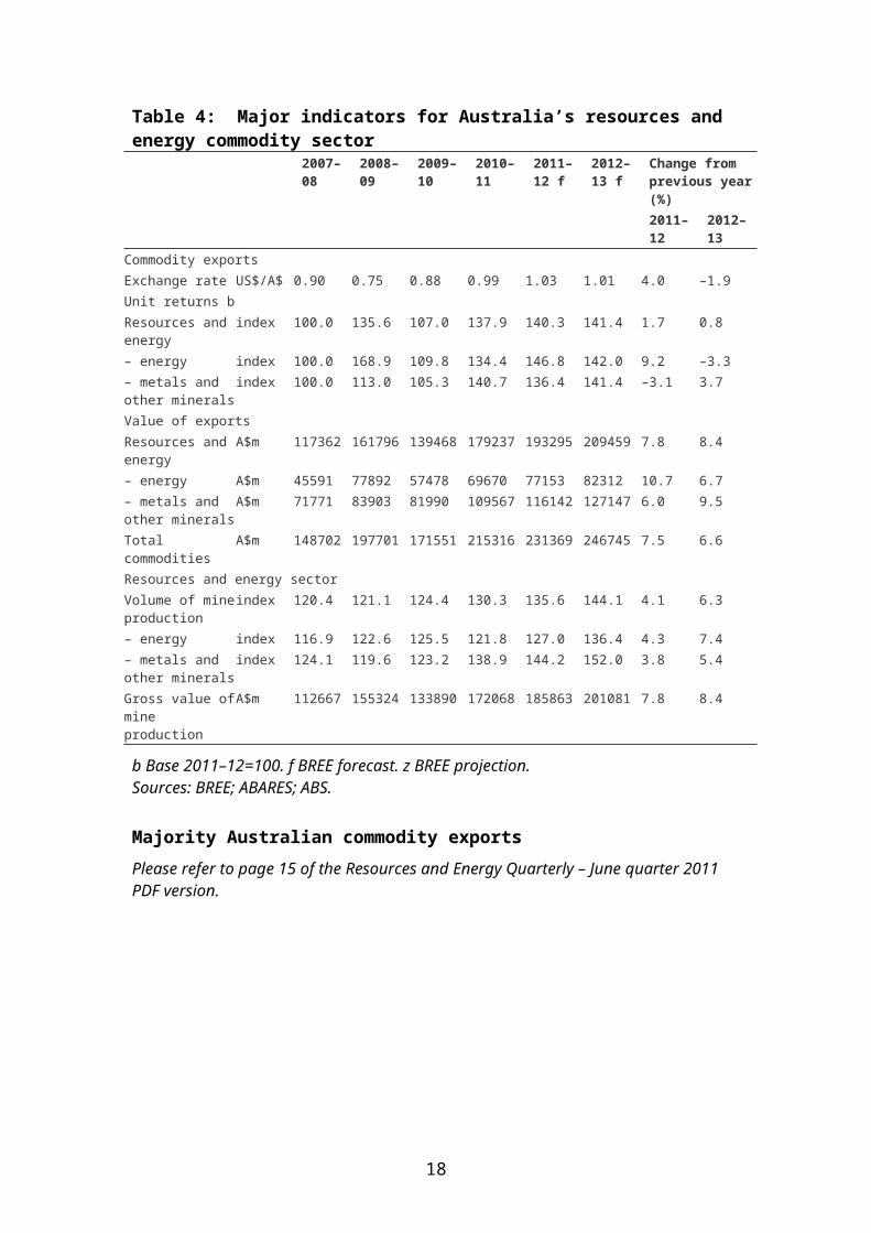
Overall, the outlook for Australian resources and energy commodities production and exports in 2012–13 remains robust (see Table 3). The major indicators for Australia’s resources and energy commodity sector are presented in Table 4. Detailed forecast and projection for major energy and minerals commodities are outlined in the following Resources Outlook and Energy Outlook sections.

Table 3: Australia’s resources and energy commodity exports, by selected

commodities

Volume Value2010–11 2011–12 f growth % 2010–11 2011–12 f growth %

Alumina kt 16942 19416 14.6 $m 5507 7144 29.7

Aluminium kt 1713 1563 –8.8 $m 3839 3374 –12.1

Copper kt 884 974 10.2 $m 8418 9043 7.4

Gold t 331 361 9.1 $m 15558 19722 26.8

Iron ore Mt 463 510 10.2 $m 62788 66936 6.6

Nickel kt 240 258 7.5 $m 3902 4138 6.0

Zinc kt 1555 1571 1.0 $m 2263 2331 3.0

LNG Mt 19 23 21.1 $m 12392 16037 29.4

Metallurgical coal Mt 142 161 13.4 $m 30310 29682 –2.1

Thermal coal Mt 159 179 12.6 $m 17358 18590 7.1

Oil ML 19167 19389 1.2 $m 13012 13319 2.4

12

Volume Value2010–11 2011–12 f growth % 2010–11 2011–12 f growth %

Uranium t 7217 7860 8.9 $m 732 799 9.2

f BREE forecast.Sources: BREE; ABS.

Table 4: Major indicators for Australia’s resources and energy commodity sector

2007–08

2008–09

2009–10

2010–11

2011–12 f

2012–13 f

Change from previous year (%)2011–12

2012–13

Commodity exports Exchange rate US$/A$ 0.90 0.75 0.88 0.99 1.03 1.01 4.0 –1.9Unit returns b Resources and energy

index 100.0 135.6 107.0 137.9 140.3 141.4 1.7 0.8

– energy index 100.0 168.9 109.8 134.4 146.8 142.0 9.2 –3.3– metals and other minerals

index 100.0 113.0 105.3 140.7 136.4 141.4 –3.1 3.7

Value of exportsResources and energy

A$m 117362 161796 139468 179237 193295 209459 7.8 8.4

– energy A$m 45591 77892 57478 69670 77153 82312 10.7 6.7– metals and other minerals

A$m 71771 83903 81990 109567 116142 127147 6.0 9.5

Total commodities A$m 148702 197701 171551 215316 231369 246745 7.5 6.6Resources and energy sectorVolume of mine production

index 120.4 121.1 124.4 130.3 135.6 144.1 4.1 6.3

– energy index 116.9 122.6 125.5 121.8 127.0 136.4 4.3 7.4– metals and other minerals

index 124.1 119.6 123.2 138.9 144.2 152.0 3.8 5.4

Gross value of mine production

A$m 112667 155324 133890 172068 185863 201081 7.8 8.4

b Base 2011–12=100. f BREE forecast. z BREE projection.Sources: BREE; ABARES; ABS.

Majority Australian commodity exports


13

Energy outlook

Oil

Nina Hitchins

Oil prices higher over the short term

Crude oil prices eased in April and May 2012, and the Brent-WTI differential narrowed. In May the WTI price averaged US$95 a barrel and the Brent price averaged US$110, around 7 per cent lower than the average for the March quarter 2012 (see Figure 1). Lower prices reflected perceived easing of tensions in the Middle East, European sovereign debt concerns, slowing economic growth in China, and increasing OECD stocks.

The WTI price is forecast to average US$96 a barrel in 2012 and US$102 a barrel in 2013. The Brent price is forecast to average US$111 a barrel in 2012 and US$113 a barrel in 2013. Increasing oil consumption and persistently low OPEC spare capacity will underpin increases in oil prices.

OPEC spare capacity has continued to fall since the December quarter 2011. In May 2012, it averaged 3.1 million barrels a day, or around 8 per cent of OPEC production. Lower OPEC spare capacity reflected an incremental increase of OPEC crude production of 1 million barrels a day, relative to the end of 2011. Increased production offset expansions in capacity, particularly in Libya. OPEC spare capacity is expected to remain low for the remainder of 2012 and 2013, as a result of increasing OPEC production. Low OPEC spare capacity is expected to support higher prices.

There are several risks to the oil price forecast throughout 2012 and 2013. Deteriorating market sentiment with regard to the euro zone, and weaker than assumed economic growth in China could reduce world oil consumption and put downward pressure on prices. Alternatively, escalating tensions in the Middle East including those between the international community and Iran could reduce apparent availability of supply and support higher than forecast prices.

Figure 1: WTI and Brent oil prices


Growth in world consumption forecast to accelerate in 2013

World oil consumption is forecast to increase by 1 per cent in 2012 to 90.1 million barrels a day. In 2013, economic activity is assumed to pick-up and world oil consumption is forecast to increase by 1.5 per cent to 91.5 million barrels a day (see

14

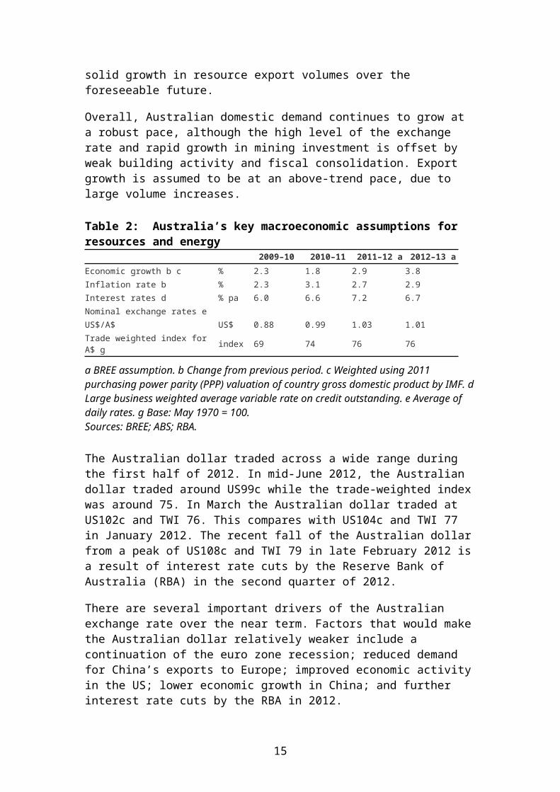
Figure 2). Increases in non-OECD consumption are expected to offset moderate falls in OECD consumption.

Consumption in the OECD is forecast to fall 0.8 per cent in 2012 to 45.3 million barrels a day. Lower consumption in North America and Europe is forecast to offset increases in the OECD Pacific (Japan, the Republic of Korea and Australasia). Increases in OECD Pacific oil consumption are forecast to be supported by oil-fired electricity generation in Japan. Oil-fired electricity generation will be relied on to bridge the gap as a result of the temporary shutdown of Japan’s nuclear industry. In 2013, OECD oil consumption is forecast to remain relatively unchanged. Structural declines in the oil use intensity of OECD economies are forecast to be offset by stronger economic growth.

Consumption in non-OECD economies is forecast to increase by 3 per cent in both 2012 and 2013 to average 46.3 million barrels a day in 2013. A third of non-OECD growth is forecast to be attributable to China. Assumed weaker economic growth during 2012 will underpin lower growth in China’s oil consumption, which is forecast to slow to 4 per cent, down from 5 per cent in 2011. In 2013, China’s oil consumption growth is forecast to rebound to 5 per cent and average 10.4 million barrels a day.

Figure 2: World oil consumption


OPEC to underpin forecast increases in production

World oil production is forecast to increase by 2 per cent in 2012 and 2013 to 91.5 million barrels a day in 2013 (see Figure 3). Non-OPEC production is forecast to increase by around 1 per cent in both 2012 and 2013 and account for a quarter of the incremental increases in world production during the outlook period.

Persistent unplanned outages during the first five month of 2012 are forecast to moderate growth in non-OPEC production during 2012. Outages continue to occur in the North Sea. Production in the UK and Norway is forecast to decrease in 2012 as a result of scheduled and unplanned maintenance.

North America’s oil production is forecast to increase by 4 per cent in 2012, offsetting declines in non-OPEC Middle East, Africa and Europe. US oil production is forecast to increase 6 per cent in 2012 and 2 per cent in 2013 to average 8.8 million barrels a day. Increases in ‘tight oil’ production, primarily from the Bakken, Nicobara and Eagle Ford formations, are forecast to offset lower production from maturing conventional fields in Alaska and California. Oil production in Canada is forecast to slow to 3 per cent in 2012, from 4 per cent in 2011, reflecting lower production estimates from Syncrude Canada, and planned maintenance from the Sea Rose floating production storage and offloading (FPSO) and Terra Tonva FPSO. In 2013,

15

Canada’s oil production is expected to increase by 4 per cent to average 3.8 million barrels a day.

Latin America’s oil production is forecast to increase by 3 per cent in 2012 and 5 per cent in 2013. Increases are forecast to be underpinned by the development of several new projects in Brazil such as Petrobras’ Parque das Beleias and Roncador module 4, and Chevron’s Papa-Terra.

OPEC oil production is forecast to increase by 3 per cent in 2012 and 2013 to average 37.9 million barrels a day in 2013. Increases in OPEC production are forecast to be underpinned by growth in the production of natural gas liquids, while OPEC crude oil production is forecast to increase by 2 per cent a year.

Figure 3: World oil supply


Australia’s production and exports

Australia’s production of crude oil and condensate is forecast to contract by 8 per cent in 2011–12, relative to 2010–11, to total 22.8 gigaliters. Lower production reflects planned maintenance on the North West Shelf for a redevelopment project, multiple unplanned shut-ins throughout the Carnarvon basin during cyclone season, and declines from maturing fields. Output from the Kitan project in the Bonaparte Basin, which commenced in October 2011, is expected to partially offset these declines. In 2012–13, Australia’s crude oil and condensate production is forecast to increase by 1 per cent as a result of the commencement of crude production from the Montara/Skua project and condensate from the Kipper gas project.

Australia’s exports of crude oil and condensate are forecast to follow a similar profile to production. Exports are forecast to contact by 2 per cent in 2011–12, and increase by 1 per cent in 2012–13 to total 19.4 gigalitres. The value of Australian oil exports is forecast to increase to $13.3 billion in 2012–13, reflecting forecast higher oil prices (see Figure 4).

Figure 4: Australia’s crude oil and condensate exports


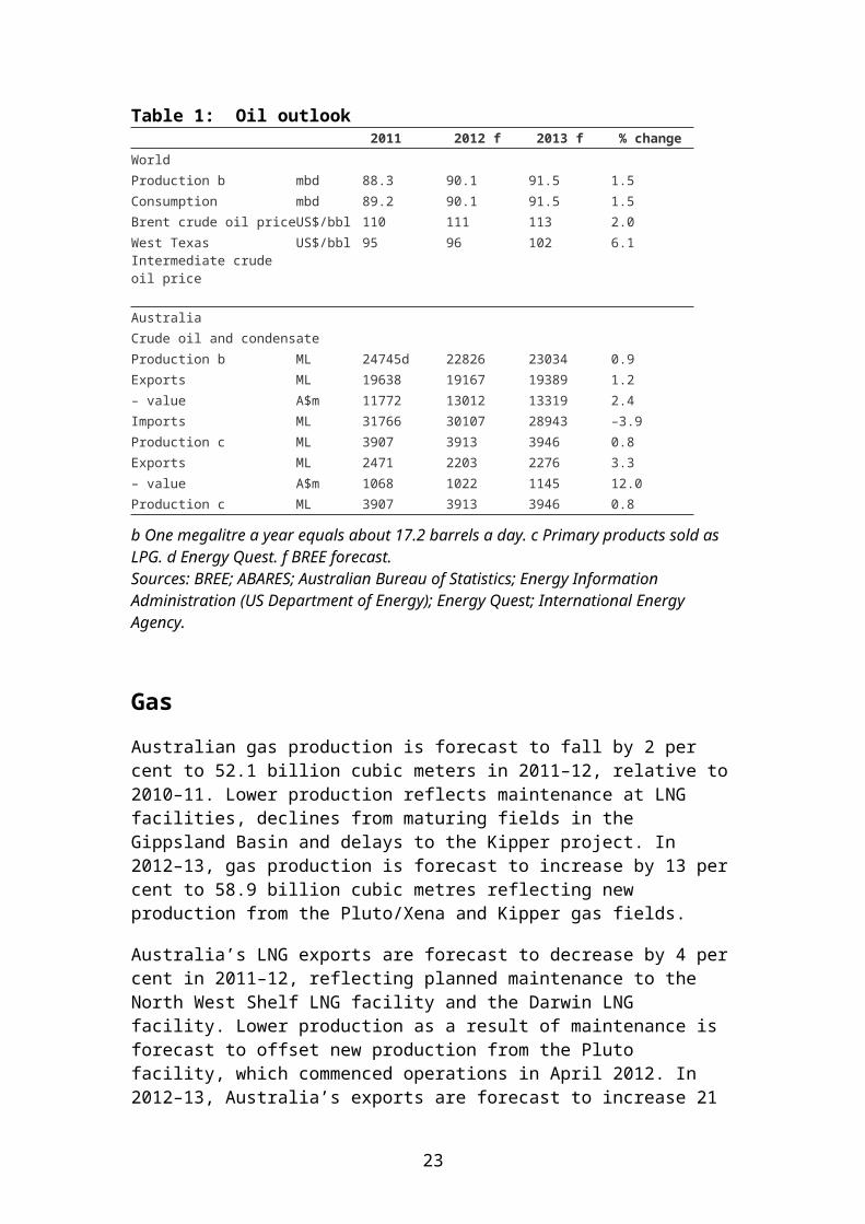
Table 1: Oil outlook2011 2012 f 2013 f % change

WorldProduction b mbd 88.3 90.1 91.5 1.5Consumption mbd 89.2 90.1 91.5 1.5Brent crude oil price US$/bbl 110 111 113 2.0West Texas Intermediate crude oil price

US$/bbl 95 96 102 6.1

16

2011 2012 f 2013 f % changeAustraliaCrude oil and condensateProduction b ML 24745d 22826 23034 0.9Exports ML 19638 19167 19389 1.2– value A$m 11772 13012 13319 2.4Imports ML 31766 30107 28943 –3.9Production c ML 3907 3913 3946 0.8Exports ML 2471 2203 2276 3.3– value A$m 1068 1022 1145 12.0Production c ML 3907 3913 3946 0.8

b One megalitre a year equals about 17.2 barrels a day. c Primary products sold as LPG. d Energy Quest. f BREE forecast.Sources: BREE; ABARES; Australian Bureau of Statistics; Energy Information Administration (US Department of Energy); Energy Quest; International Energy Agency.

Gas

Australian gas production is forecast to fall by 2 per cent to 52.1 billion cubic meters in 2011–12, relative to 2010–11. Lower production reflects maintenance at LNG facilities, declines from maturing fields in the Gippsland Basin and delays to the Kipper project. In 2012–13, gas production is forecast to increase by 13 per cent to 58.9 billion cubic metres reflecting new production from the Pluto/Xena and Kipper gas fields.

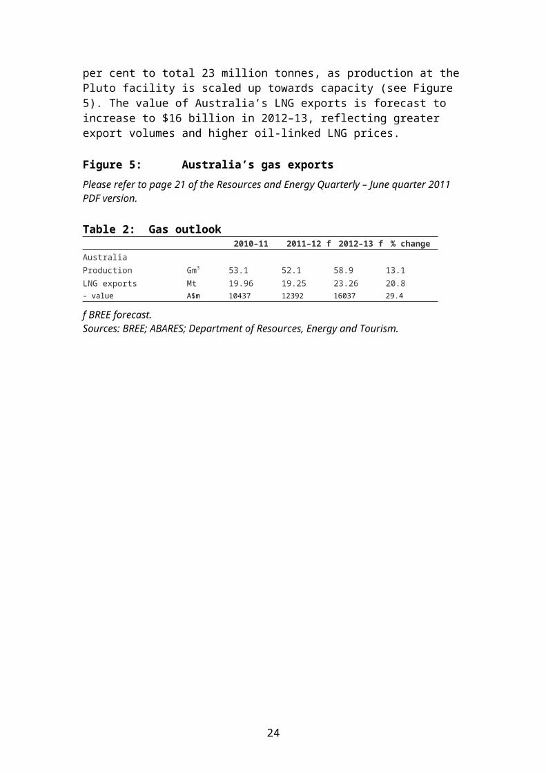
Australia’s LNG exports are forecast to decrease by 4 per cent in 2011–12, reflecting planned maintenance to the North West Shelf LNG facility and the Darwin LNG facility. Lower production as a result of maintenance is forecast to offset new production from the Pluto facility, which commenced operations in April 2012. In 2012–13, Australia’s exports are forecast to increase 21 per cent to total 23 million tonnes, as production at the Pluto facility is scaled up towards capacity (see Figure 5). The value of Australia’s LNG exports is forecast to increase to $16 billion in 2012–13, reflecting greater export volumes and higher oil-linked LNG prices.

Figure 5: Australia’s gas exports


Table 2: Gas outlook2010–11 2011–12 f 2012–13 f % change

AustraliaProduction Gm3

53.1 52.1 58.9 13.1LNG exports Mt 19.96 19.25 23.26 20.8– value A$m 10437 12392 16037 29.4

f BREE forecast.Sources: BREE; ABARES; Department of Resources, Energy and Tourism.

17

Thermal coal

Tom Shael

Prices

Thermal coal contract prices were settled in early June at around US$115 a tonne for Japanese Financial Year (JFY) 2012 with several Japanese power utilities (see Figure 1). This price represents a decrease of about 12 per cent from the JFY 2011 price. In line with lower expected economic growth in China, India and the European Union (EU), thermal coal spot prices are around a US$30 a tonne discount from the JFY 2012 contract price.

Figure 1: JFY thermal coal prices


World trade

The world thermal coal seaborne trade in 2012 is forecast to increase by around 4 per cent, relative to 2011, to total 871 million tonnes. The global seaborne trade in 2013 is forecast to increase by a further 5 per cent, relative to 2012, to total 919 million tonnes.

Imports

Growth in imports in 2012 and 2013 will primarily be supported by increased demand from Asia. Higher electricity demand associated with robust economic growth in emerging economies is expected to be a key driver of demand. India is forecast to contribute the most to this growth, growing by 14 per cent in 2012, relative to 2011, and by a further 17 per cent in 2013 to total 104 million tonnes. China is forecast to increase its seaborne imports by 6 million tonnes in both 2012 and 2013 to total 145 and 151 million tonnes, respectively.

In 2012, imports into the EU are forecast to fall by 1 million tonnes to 160 million tonnes. This expected decline is a result of assumed weak economic growth and lower electricity demand stemming from the euro zone crisis. In 2013 an assumed increase in economic growth in Europe will contribute to a 3 million tonnes increase in import demand into the EU from 2012 levels.

Japan’s imports of thermal coal are forecast to increase slightly in 2012 to total 128 million tonnes in response to the temporary shutdown of its nuclear electricity generation capacity. Japan’s imports in 2013 are forecast to increase by a further 1 million tonnes, to 129 million tonnes.

18

Exports

Higher import demand across 2012 and 2013 is forecast to be supplied with higher exports from Australia, Indonesia and Colombia. In 2012, Australia’s exports are forecast to increase by 11 per cent to 164 million tonnes. This represents a volume increase in Australia of 16 million tonnes that will be underpinned higher production rates from existing mines and recently commissioned operations. Increased volumes are forecast from: Xstrata’s Mangoola mine (annual capacity of 8 million tonnes), stage 1 of Yancoal’s Moolarben mine (8 million tonnes) and Peabody Energy’s expansion of its Wilpinjong operation (additional annual capacity of 2–3 million tonnes). In 2013, Australia’s exports are forecast to increase by a further 17 per cent to total 192 million tonnes. This large increase will be supported by production from soon-to-be-commissioned mines that include the Hunter Valley Operations Expansion (6 million tonnes) and Narrabri Coal Project stage 2 expansion (4.5 million tonnes).

In 2012, Indonesia’s exports are forecast to increase by 2 per cent to total 308 million tonnes, before increasing by a further 4 per cent in 2013 to 319 million tonnes. This growth is expected to be supported by increased production from PT Bumi’s, PT Adaro Energy’s and PT Indika Energy’s coal mines along with output expansions from mines located in the East Kalimantan region.

Exports from Colombia are forecast to remain relatively unchanged in 2012, before increasing by 6 million tonnes to total 82 million tonnes in 2013. Colombia’s higher thermal coal exports in 2013 should be supported by expansions to capacity at mines in the La Guajira and César regions.

In 2012, exports from the US are forecast to increase by 16 per cent, relative to 2011, to total 36 million tonnes. The sharp upturn is expected to be a response to low domestic demand arising from the cheap and plentiful supply of natural gas. Domestic production of thermal coal in the second half of 2012, however, is expected to decline sharply as producers respond to falling domestic demand and lower export prices. Despite the fall in production, exports should be robust as producers sell their stocks before placing mines on care and maintenance. Exports in 2013 are forecast to fall relative to 2012 levels to total 31 million tonnes.

Australia

In 2011–12, Australia’s thermal coal production is forecast to increase by 8 per cent, relative to 2010–11, to total 223 million tonnes. Production in 2012–13 is forecast to increase by a further 9 per cent, to 244 million tonnes.

In line with higher production, exports of thermal coal in 2011–12 and 2012–13 are forecast to be 159 million tonnes and 179 million tonnes, respectively. The growth in export volumes will be supported by increased port capacity associated with the start-up of the Port Waratah Coal Services’ Kooragang Island Coal Terminal expansion (11 million tonnes a year), the X50 expansion at Abbot Point (25 million

19

tonnes a year) and higher throughput at the Newcastle Coal Infrastructure Group’s Coal Terminal.

In 2011–12 the value of Australia’s thermal coal exports is forecast to increase by 24 per cent, relative to 2010–11, to total $17.4 billion primarily as a result of higher export volumes. In 2012–13, forecast higher export volumes will outweigh lower contract prices for JFY 2012 that should result in export earnings increasing to $18.6 billion.

Figure 2: Australia’s thermal coal exports


Table 1: Thermal coal outlook2011 2012 f 2013 f % change

WorldThermal coal Contract prices b US$/t 130 115 100 –13.0Coal trade Mt 837 871 919 5.4ImportsAsia Mt 569 599 632 5.4– China Mt 139 145 151 4.1– Chinese Taipei Mt 67 68 69 1.8– India Mt 78 89 104 16.9– Japan Mt 125 128 129 0.4– Korea, Rep. of Mt 97 99 102 3.0– Malaysia Mt 20 21 22 3.9– other Asia Mt 43 49 55 12.4Europe Mt 204 205 210 2.4– European Union 27 c Mt 161 160 163 1.6– other Europe Mt 43 45 48 5.5Other Mt 64 67 77 14.3ExportsAustralia Mt 148 164 192 18.5China Mt 13 12 12 2.5Colombia Mt 75 76 82 7.8Indonesia Mt 302 308 319 3.6Russian Federation Mt 97 99 99 0.6South Africa Mt 66 69 72 3.7United States Mt 31 36 31 –13.9Other Mt 105 108 111 2.3

2010–11 2011–12 f 2012–13 f % changeAustraliaProduction Mt 206.1s 223.4 244.3 13.8Exports Mt 143.3 159.0 179.3 19.6– value A$m 13956 17358 18590 13.8

b Japanese Fiscal Year, starting April 1, fob Australia basis, BREE Australia–Japan average contract price assessment. For steaming coal with a calorific value of 6700 kcal/kg (gross air dried. c Regarded as 27 countries for all years. f BREE forecast. s BREE estimate.Sources: BREE; ABARES; International Energy Agency; Coal Services Pty Ltd; Queensland Department of Mines and Energy.

20

Resources outlook

Steel and steel-making raw materials

Rubhen Jeya

Contract prices

In the first quarter of 2012, iron ore spot prices averaged around US$135 a tonne for 62 per cent iron ore content free on board (FOB) Australia, an increase of 4 per cent from the previous quarter. The increase in spot prices was largely due to the effect of weather-related supply disruptions in Western Australia and Brazil, and restocking in China. In the June quarter 2012, spot prices have averaged around US$135 a tonne, but prices in the second half of the June quarter have fallen. For 2012 as a whole, contract prices are forecast to average around US$136 a tonne (see Figure 1). In 2013, contract prices are assumed to moderate to average around US$131 a tonne. The forecast decrease in prices is a result of projected increased supply from Australia and Brazil, and a moderation of growth in import demand.

The June quarter 2012 contract prices for high-quality hard coking coal settled at around US$210 a tonne. This represents an 11 per cent decline from the March quarter contract price primarily due to weaker import demand. The September quarter contract prices are expected to settle higher at around US$225 a tonne partly as a result of reduced production associated with industrial action at BHP Billiton-Mitsubishi Alliance (BMA) mines in Queensland. For 2012 as a whole, contract prices for high-quality hard coking coal are forecast to average around US$221 a tonne. Hard coking coal contract prices are projected to moderate through 2013, underpinned by supply increases from Australia, Canada, Mongolia and Mozambique.

Figure 1: Raw material contract prices, FOB Australia


Steel

World steel consumption

In 2012, world steel consumption is forecast to increase by 3 per cent, relative to 2011, to 1.5 billion tonnes, supported by demand from the construction of infrastructure projects in a number of developing economies. Despite robust growth in steel consumption, relative to 2011, the rate of growth is forecast to slow, in line with assumed weaker economic growth across the OECD and China. In 2013, world steel consumption is forecast to increase by about 4 per cent, relative to 2012, to total 1.55 billion tonnes (see Table 1).

21

In China, strong growth in steel consumption has been supported by the construction of public infrastructure and manufacturing of consumer durables. In 2012 and 2013, China’s steel consumption is forecast to increase by 4 per cent each year, to total 648 million tonnes and 676 million tonnes, respectively. Downward revisions have been made to China’s steel consumption growth from the March 2012 Resource and Energy Quarterly due to a reduction in assumed domestic economic growth.

In India, steel demand for infrastructure construction and higher consumption of consumer durables is expected to underpin a 7 per cent increase in steel consumption in 2013. In the European Union (EU), steel consumption is forecast to remain largely unchanged in 2012 and 2013 due to an assumed contraction in economic growth over the period.

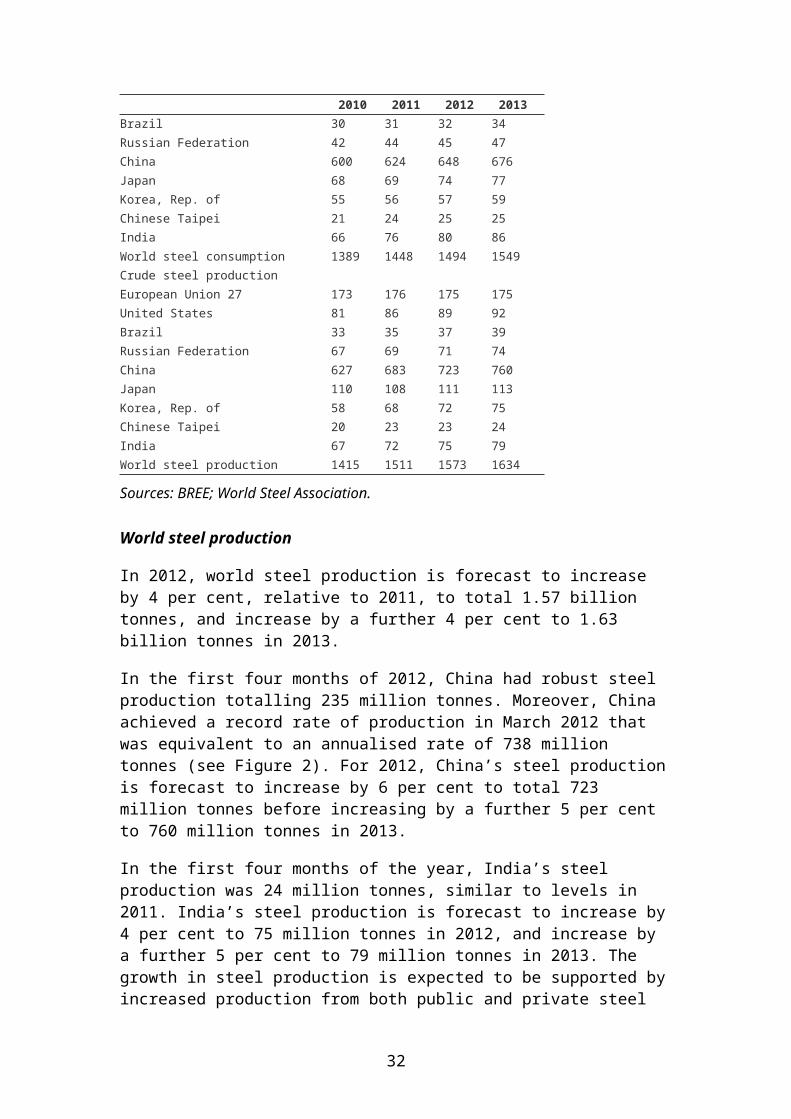
Table 1: World steel consumption and production (Mt)2010 2011 2012 2013

Crude steel consumptionEuropean Union 27 160 162 162 162United States 90 94 95 97Brazil 30 31 32 34Russian Federation 42 44 45 47China 600 624 648 676Japan 68 69 74 77Korea, Rep. of 55 56 57 59Chinese Taipei 21 24 25 25India 66 76 80 86World steel consumption 1389 1448 1494 1549Crude steel productionEuropean Union 27 173 176 175 175United States 81 86 89 92Brazil 33 35 37 39Russian Federation 67 69 71 74China 627 683 723 760Japan 110 108 111 113Korea, Rep. of 58 68 72 75Chinese Taipei 20 23 23 24India 67 72 75 79World steel production 1415 1511 1573 1634

Sources: BREE; World Steel Association.

World steel production

In 2012, world steel production is forecast to increase by 4 per cent, relative to 2011, to total 1.57 billion tonnes, and increase by a further 4 per cent to 1.63 billion tonnes in 2013.

In the first four months of 2012, China had robust steel production totalling 235 million tonnes. Moreover, China achieved a record rate of production in March 2012 that was equivalent to an annualised rate of 738 million tonnes (see Figure 2). For 2012, China’s steel production is forecast to increase by 6 per cent to total 723

22

million tonnes before increasing by a further 5 per cent to 760 million tonnes in 2013.

In the first four months of the year, India’s steel production was 24 million tonnes, similar to levels in 2011. India’s steel production is forecast to increase by 4 per cent to 75 million tonnes in 2012, and increase by a further 5 per cent to 79 million tonnes in 2013. The growth in steel production is expected to be supported by increased production from both public and private steel producers. In the EU, steel production in 2012 and in 2013 is forecast to remain largely unchanged, relative to 2011, at around 175 million tonnes. This is due to the steel industry operating well below capacity.

Figure 2: Monthly world steel production


Iron ore

In 2012, world trade in iron ore is forecast to increase by 5 per cent from 2011 to 1.1 billion tonnes. World trade in iron ore in 2013 is forecast to increase by a further 6 per cent to 1.2 billion tonnes (see Table 2).

Iron ore imports

In 2012, China’s imports of iron ore are forecast to increase by 8 per cent, compared with 2011, to total 699 million tonnes. In 2013, imports are forecast to increase by a further 4 per cent to 724 million tonnes. The increase in iron ore imports will be underpinned by continued growth in steel production and domestic iron ore consumption growth that will continue to outpace the rise in domestic production.

Iron ore imports into the EU in 2012 and 2013 are forecast to remain steady at around 137 million tonnes. The lack of growth in iron ore imports in 2012 and 2013 reflects unchanged levels of steel production in these years.

Imports by other major iron ore consumers, such as the Republic of Korea and Japan, are expected to continue to increase in line with modest growth in steel production in 2012 and 2013.

Table 2: World iron ore trade (Mt)2010 2011 2012 2013

Iron ore importsEuropean Union 27 133 136 137 137Japan 134 128 134 136China 619 645 699 724Korea, Rep. of 56 64 67 72Chinese Taipei 19 22 23 23World imports 1051 1075 1133 1204Iron ore exports

23

2010 2011 2012 2013Australia 402 439 479 535Brazil 311 313 326 361India 96 63 48 53Canada 33 34 36 37South Africa 48 54 58 64West Africa (Guinea & Mauritania) 11 12 14 15World exports 1051 1075 1133 1204

Source: BREE.

Iron ore exports

In 2012, Australia’s exports of iron ore are forecast to increase by 9 per cent from the previous year to total 479 million tonnes. The increase will be supported by capacity expansions at a number of mines including those operated by Rio Tinto, and the ramp up of production at BHP Billiton’s Rapid Growth Project 5. In 2013, Australia’s iron ore exports are forecast to increase by a further 12 per cent, supported by new mine operations scheduled to start in late 2012 and 2013. These include: Fortescue’s Chichester Hub (capacity of 40 million tonnes per year), CITIC Pacific Mining’s Sino Iron Project (capacity of 28 million tonnes per year) and Rio Tonto’s Hope Downs 4 (capacity of 15 million tonnes per year) and Western Turner Syncline 2 (capacity of 9 million tonnes per year).

In the financial year 2011–12, Australia’s export volumes are forecast to increase by 14 per cent, relative to 2010–11, to total 463 million tonnes. The value of Australia’s iron ore exports in 2011–12 is forecast to increase by 8 per cent to $63 billion, compared with 2010–11.

In 2012–13, Australia’s iron ore export volumes are forecast to increase by 10 per cent, relative to 2011–12, to total 510 million tonnes. The value of iron ore export values in 2013–13 is forecast to increase by 7 per cent to $67 billion (see Figure 3). This value is largely attributable to an increase in export volumes that will outweigh a slight decline in prices from the previous corresponding period.

In 2012, Brazil’s iron ore exports are forecast to increase by 4 per cent, relative to 2011, to total 326 million tonnes. Brazil’s exports in 2013 are forecast to increase by 11 per cent year on year to total 361 million tonnes. The slower growth in 2012, relative to 2013 is largely attributable to weather related production losses in the first quarter of 2012. The increase in exports in 2013 is largely a result of the increase in production at a number of mines in the south-eastern Systems and at Carajas where production is expected to ramp up from recent expansions and also from increased production at existing mines as these return to normal levels of production. A large proportion of these exports are expected to be sourced from expansions to Vale’s operations.

Figure 3: Australia’s iron ore exports


24

Metallurgical coal

In 2012, global trade in metallurgical coal is forecast to increase by 6 per cent to 286 million tonnes. World metallurgical trade is forecast to increase by a further 3 per cent to 296 million tonnes in 2013 supported by import growth in China and India (see Table 3).

Metallurgical coal imports

In the first three months of 2012, China increased its imports of metallurgical coal by around 17 per cent from the previous quarter. The higher volumes were sourced from increased exports from Australia and Mongolia. For 2012 as a whole, China’s metallurgical coal imports are forecast to increase by 15 per cent to 53 million tonnes, partly as a result of restocking at steel mills, but also from forecast robust steel production throughout 2012. In 2013, China’s imports are forecast to increase by a further 6 per cent to 56 million tonnes, as metallurgical coal consumption outpaces growth in domestic production.

The other major source of metallurgical coal import growth is India, where imports are forecast to increase by 6 per cent in 2012 to total 34 million tonnes, and by a further 6 per cent to 36 million tonnes in 2013.

Imports by the EU are forecast to remain largely unchanged in 2012 and 2013 from 2011 at around 46 million tonnes. The lack of growth in 2012 and 2013 is consistent with stagnant steel production forecast for these years.

Table 3: World metallurgical coal trade (Mt)2010 2011 2012 2013

Metallurgical coal importsEuropean Union 27 45 45 46 46Japan 58 55 55 56China 48 46 53 56Korea, Rep. of 28 34 34 35Chinese Taipei 5 7 7 7India 30 32 34 36Brazil 12 13 14 15World imports 273 270 286 296Metallurgical coal exportsAustralia 159 133 149 163Canada 28 30 33 35United States 51 55 51 46Russian Federation 14 17 18 20World exports 273 270 286 296

Source: BREE.

Metallurgical coal exports

Australia is the largest exporter of metallurgical coal in the world. Australia’s metallurgical coal exports in 2012 are forecast to increase by 12 per cent to 149

25

million tonnes as mines in Queensland recover from flood-related disruptions in 2011. Exports in 2013 are forecast to increase further by 9 per cent to 163 million tonnes, underpinned by increased production from BMA mines in Queensland under the assumption that current industrial disputes conclude shortly. There is also expected to be increased production from a number of mines that are scheduled to start up in 2013, such as Peabody Energy’s Burton mine and at Anglo Coal’s Grosvenor underground mines.

In 2012, US metallurgical coal exports are forecast to decrease by 7 per cent relative to 2011 to total 51 million tonnes. Exports are forecast to decline by a further 11 per cent in 2013 to total 46 million tonnes. The decline in US metallurgical coal exports is partly a result of a decline in import demand in Europe and from the idling of a number of coal mines.

Australia’s metallurgical coal export volumes in the financial year 2011–12 are forecast to increase by 1 per cent to 142 million tonnes and this is expected to result in an increase in export earnings by 2 per cent to $30 billion. During the 2012–13, Australia’s metallurgical coal exports are forecast to increase by 13 per cent to 161 million tonnes. Despite high export volumes, earnings are forecast to decline by 2 per cent to $29.7 billion due to forecast lower contract prices for 2012–13 (see Figure 4).

Figure 4: Australia’s metallurgical coal exports


Table 4: Steel and steel-making raw materials outlook2011 2012 f 2013 f % change

WorldContract prices bIron ore c US$/t 153 136 131 –3.2Metallurgical coal d US$/t 289 221 211 –4.7

2010–11 2011–12 f 2012–13 f % changeAustraliaProductionIron and steel e s Mt 7.31 5.38 4.86 –9.7Iron ore Mt 450 509 527 3.5Metallurgical coal Mt 147 s 146 164 12.6ExportsIron and steel e s Mt 1.78 1.19 1.02 –14.3– value A$m 1 303 983 789 –19.7Iron ore Mt 407 463 510 10.3– value A$m 58387 62788 66936 6.6Metallurgical coal Mt 140 142 161 13.4– value A$m 29793 30310 29682 –2.1

b fob Australian basis, BREE Australia–Japan average contract price assessment. c Fines contract, 62% iron content basis. d High–quality hard coking coal. For example, Goonyella export coal. e Includes all steel items in ABS, Australian Harmonized Export Commodity Classification, chapter 72, ‘Iron and steel’, excluding ferrous waste and scrap and ferroalloys.

26

f BREE forecast. s BREE estimate.Sources: BREE; ABARES; International Iron and Steel Institute; Coal Services Australia; Queensland Coal Board; United Nations Conference on Trade and Development.

27

Gold

Adam Bialowas

Prices

In the March quarter of 2012, the price of gold averaged US$1690 an ounce, very close to the average price in the December quarter 2011. However, in the June quarter, the gold price has fallen from US$1670 an ounce in early April to US$1550 an ounce in late May. The decrease in the gold price over the June quarter has been in response to a re-emergence of sovereign debt issues in the euro zone which has seen a flight of capital into the US and a strengthening of the US dollar. This in turn has led to a decline in the US dollar denominated price of gold.

In 2012, the price of gold is forecast to average US$1660 an ounce, an increase of 6 per cent relative to 2011. Strong supply and demand fundamentals are expected to support the price of gold in 2012. In particular, official sector purchases represent a relatively price independent source of demand that will underpin the price of gold in 2012. Gold prices in 2013 are forecast to increase by an additional 3 per cent to US$1710 a tonne (see Figure 1). The increase in the gold price in 2013 reflects strong demand, particularly from the official sector.

Figure 1: Gold prices


Fabrication demand to remain steady

Fabrication demand comprises gold used in jewellery, electronics, dental applications, medals, coins and other industrial uses. In 2012, gold fabrication demand is forecast to increase by 2 per cent relative to 2011 to total 2808 tonnes. The modest growth in fabrication demand reflects high gold prices that are expected to dampen consumption growth in many markets. This increase is driven largely by China, where income growth has fuelled significant demand for gold jewellery. In 2013, reflecting expectations of a more stable gold price, fabrication demand for gold is expected to increase by 2 per cent to 2856 tonnes.

Official sector purchases to continue

In 2012, official sector purchases of gold are expected to remain robust at 425 tonnes, similar to levels in 2011. The levels of official sector purchases are due to the exposure of many central banks to foreign exchange risks. The recent variability of the US dollar relative to some national currencies and concerns over the euro has led to increased interest in gold as a means of diversifying central bank asset holdings. In

28

2013 the official sector is expected to remain a net purchaser of gold at a level of 400 tonnes, as uncertainty remains in financial and asset markets.

Supply to increase modestly

World gold mine production in 2012 is forecast to increase by 3 per cent, relative to 2011, to 2907 tonnes. Production is expected to increase in Canada as a result of new developments such as New Gold’s New Afton project and AuRico’s Young-Davidson operation. Gold production in Turkey is also expected to increase due to the start up of Eldorado Gold’s Efemçukuru and Alacer Gold’s copper operations.

Global gold mine production is forecast to increase in 2013 by a further 2 per cent to 2977 tonnes. Strong growth is expected to come from the Russian Federation as a result of Polyus Gold’s Verninskoye and Natalka operations. Latin America will become an increasingly important gold producing region with new mines starting up such as Newgold’s Cerro Negro operation in Argentina and Barrick’s Pueblo Viejo mine in the Dominican Republic.

Reduced availability to see scrap supply decline

In 2012 the supply of scrap is forecast to decrease by 7 per cent to 1550 tonnes. The fall in scrap supply reflects consumers’ willingness to hold gold in the absence of better alternative investments. It also reflects the decreased availability of scrap as stock levels have been run down significantly over the past four years following successive increases in gold prices. Similarly, despite a forecast price increase in 2013, the quantity of gold sourced from scrap is expected to decline by a further 6 per cent to 1450 tonnes.

Australia’s gold production to increase strongly

Australia’s gold mine production in 2011–12 is forecast to decrease by 1 per cent relative to 2010–11 to total 261 tonnes. The decrease in production is due to a number of mines taking advantage of high gold prices to target lower ore grades that would otherwise have been uneconomic to extract.

Australia’s gold mine production in 2012–13 is expected to increase by 8 per cent relative to 2010–11 to total 283 tonnes. The largest contribution to this increase is expected to come from Newcrest’s Cadia East operation with an increase in capacity of 8 tonnes a year. Other mines starting up in 2012–13 include Millennium Minerals’ Nullagine and Crocodile Gold’s Cosmo Deeps.

Australia’s gold exports consist of refined gold from domestic mine production and imports of gold dore (impure gold) and scrap gold, which are shipped to Australia and then refined into gold bullion and re–exported. In 2011–12, the volume of Australia’s gold exports is forecast to increase by 10 per cent, relative to 2010–11, to total 331 tonnes. The increase in exports is expected to be supported by a forecast increased availability of scrap and gold dore from international sources as a result of

29

continued high prices for gold. Accordingly, the value of Australia’s gold exports is forecast to rise by 20 per cent in 2011–12 to $15.6 billion (see Figure 2).

In 2012–13, increases in exports of both domestically produced gold and re-exported scrap are forecast to result in export volumes rising by 9 per cent to 361 tonnes. The value of Australia’s gold exports is forecast to increase by 27 per cent to $19.7 billion. This reflects a combination of high gold prices and increased export volumes.

Figure 2: Australia’s gold exports


Table 1: Gold outlook2011 2012 f 2013 f % change

WorldFabrication consumption t 2759 2808 2856 1.7Mine production t 2818 2907 2977 2.4– China t 371 380 390 2.6– Australia t 259 272 297 9.2– United States t 233 240 247 2.9– Russian Federation t 212 217 222 2.3– South Africa t 198 195 190 –2.6Scrap sales t 1661 1550 1450 –6.5Net stock sales t (1720) (1633) (1551) –5.0– official sector t 455 425 400 –5.9– private sector t (1271) (1214) (1161) –4.0– producer hedging t 6 (10) (10) 0.0Price b US$/oz 1569 1663 1713 3.0

2010–11 2011–12 f 2012–13 f % changeAustraliaMine production t 265 261 283 8.4Exports t 301 331 361 9.1– value A$m 13016 15558 19722 26.8Price A$/oz 1389 1624 1698 4.5

b London Bullion Market Association AM price. f BREE forecast.Note: Net purchasing and dehedging shown in brackets.Sources: BREE; ABARES; Gold Fields Mineral Services; Australian Bureau of Statistics; London Bullion Market Association.

30

Metals overview

Adam Bialowas

Metals consumption

In the March quarter 2012, global consumption of aluminium, copper and nickel increased across most large consuming regions. The increase in consumption was largely underpinned increasing consumption in China and the US. Europe's consumption of metals in the first quarter of 2012 was generally lower, relative to the corresponding period in 2011 (see Figure 1).

While China's economic growth slowed in the first quarter of 2012, relative to the corresponding quarter in 2011, it remained robust and supportive of increased metals consumption. Also supporting China's metal consumption was the restocking of depleted inventories. The growth in US metals consumption was underpinned by improvements in economic activity and industrial production. Importantly for the US economy, housing construction has started to pick up which is a large consumer of copper and aluminium. In Europe, weak economic growth across the region has resulted in lower consumption of most metals in the March quarter of 2012, with the exception of nickel.

Figure 1: March quarter consumption of base metals, 2011 vs 2012


In the June quarter 2012, uncertainty over the economic outlook is expected to result in weaker metals consumption growth in China and the US and the continued contraction of consumption in Europe. The uncertainty over potential impacts from Europe's sovereign debt crisis has resulted in lower consumer and business confidence. Many European economies are now in recession, which is expected to result in lower demand for metal-intensive products. In China, reduced economic activity in one of its major trading partners, Europe, is expected to result in a slowing in manufacturing activity. This in turn will lead to a slowing of economic growth and manufacturing activity resulting in a slowing of demand for metals. These developments have been reflected in price movements over the past quarter (see Figure 2). All metals prices have fallen over the course of the quarter with the largest decreases being for copper (16 per cent) and nickel (13 per cent).

Figure 2: Index of daily base metal prices


31

Over the second half of 2012 and in 2013, metals consumption growth is expected to be subdued relative to growth rates in 2011 and 2010. Consumption growth in 2013 may start to increase associated with assumed stronger economic growth, particularly in Europe. In China the implementation of a stimulus package would be supportive of increased metals consumption. In the US, low energy prices, particularly for coal and gas, could be supportive of increased manufacturing activity, which in turn would support metals demand.

Metals prices

In 2012, most metals prices are forecast to decrease relative to 2011, before increasing modestly in 2013. The extent to which metals prices fall in 2012, relative to 2011 is linked to two factors. Firstly, metals price decreases will reflect market expectations for future consumption. If the economic conditions around the world worsen, metals prices would likely continue to fall.

Related to the economic outlook are movements of the US dollar. Economic uncertainty could lead to a flight of capital to US dollar denominated safe haven or quality investments. This would result in an appreciation of the value of the US dollar against other currencies, which in turn would reduce the purchasing power of non US denominated currencies place further downward pressures on commodity prices.

The second factor is the extent which metals production costs have increased over the past decade, which could limit price decreases. Capital and operating costs have been impacted by increases in the costs of plant and machinery, labour and other inputs. Additionally, high prices for many base metals in the preceding few years provided incentives for producers to mine progressively lower grade ores and/or deposits that are technically more difficult to mine. If prices continue to fall, the higher extraction and refining costs will cause a number of mines will become unprofitable and will be shut down. This in turn will lead to a reduction in supply which will provide some support for commodity prices.

In 2013, prices for most metals are forecast to increase as economic growth and consumption increase and under the assumption that the uncertainty that currently surrounds the economic outlook starts to ease (see Figure 3).

Figure 3: Index of quarterly base metal prices


32

Copper

Adam Bialowas

Prices to decline in 2012 and 2013

In the March quarter of 2012 the price of copper averaged $US8300 a tonne. This represented an 11 per cent increase compared to the December quarter 2011 but a 14 per cent fall when compared to the March quarter 2011.

In the June quarter 2012 the copper price declined from US$8580 a tonne in early April to US$7520 a tonne in late-May. For 2012 as a whole, copper prices are forecast to average $US7860 a tonne, a decrease of 11 per cent relative to 2011 (see Figure 1). The decrease in prices over the June quarter and compared with 2011 is due to weaker market sentiment towards the outlook for global copper consumption. The weakening of market sentiment has occurred because of recent weaker Chinese economic data and uncertainty over the outlook for a number of large European economies.

Copper prices in 2013 are forecast to decrease by a further 3 per cent to $US7608 a tonne. Growth in world refined copper production is expected to outpace growth in consumption in 2013, placing downward pressure on prices.

Figure 1: Copper prices and stocks


Consumption to increase steadily

World consumption of refined copper in 2012 is forecast to increase by 4 per cent, relative to 2011, to total 20.3 million tonnes. A large proportion of this increase is expected to occur in China where copper consumption is forecast to increase by 8 per cent in 2012, to 8.5 million tonnes. Other countries where copper consumption is forecast to grow include: the US (up 4 per cent to 1.8 million tonnes), the Republic of Korea (up 6 per cent to 792 000 tonnes) and Brazil (up 4 per cent to 439 000 tonnes). By contrast, many OECD countries such as Germany and Italy are expected to register stagnant or decreases in consumption in 2012.

In 2013 world refined copper consumption is forecast to increase by a further 5 per cent, to 21.4 million tonnes. The strongest growth in consumption is forecast to occur in China (up 8 per cent to 9.2 million tonnes), supported by growth in other non-OECD economies such as Brazil (up 8 per cent to 475 000 tonnes), the Russian Federation (up 4 per cent to 720 000 tonnes) and India (up 5 per cent to 438 000 tonnes).

33

Mine production to grow strongly in 2013

In 2012 world copper production is forecast to increase by 2 per cent relative to 2011 to 16.5 million tonnes. The increase in copper production assumes an easing of industrial and labour disputes in Latin America and Indonesia which adversely impacted copper production in 2011. Africa’s copper production in 2012 is also forecast to increase, relative to 2011, underpinned by new operations such as First Quantum Minerals’ Kansanshi operation (annual capacity of 400 000 tonnes) and a continued ramp up to full production at Vedanta Resource’s Konkola operation (200 000 tonnes), both of which are located in Zambia.

World copper mine production in 2013 is expected to increase a further 9 per cent to 18 million tonnes, with growth occurring in Chile (up 4 per cent to 6 million tonnes) and Peru (up 7 per cent to 1.5 million tonnes). In Chile, Antofagasta’s Esperanza mine (annual capacity of 210 000 tonnes) is continuing to ramp up towards full production while in Peru Chinalco’s Tormocho mine (200 000 tonnes) is expected to commence production in 2013. Australia’s copper production in 2013 is forecast to increase by 16 per cent to 1.2 million tonnes supported by an expansion of the Cadia East mine and the start up of the Nullagine and DeGrussa mines.

Refined production to follow growth in mine production

In 2012 world refined production is forecast to increase by only 2 per cent to 20.2 million tonnes. Increases in world refined copper production are expected to continue to be constrained by a shortage of concentrates, rather than a lack of refining capacity. Growth is expected to come from Africa, particularly the Democratic Republic of Congo and Zambia, both of which have new mines which employ the solvent-extraction electro-winning (SX-EW) mining technique. China is forecast to remain the world’s largest producer of refined copper, increasing production by 8 per cent to 5.6 million tonnes. In 2013, as a result of improved concentrate availability, refined copper production is expected to grow by 6 per cent to 21.5 million tonnes. Increased production is expected to occur mainly in China and Africa.

Australia’s copper production and exports to increase

In 2011–12, Australia’s copper mine production is forecast to increase by 2 per cent, relative to 2010–11, to 971 000 tonnes. Increased production will be supported by the start up of Hillgrove Resources’ Kanmantoo mine (annual capacity of 20 000 tonnes) and Kimberley Metals’ Mineral Hill operation (10 000 tonnes). These new operations will more than offset the effects of the closure of Kagara Mining’s operation (annual capacity of 20 000 tonnes) in early 2012.

Australian copper mine production in 2012–13 is forecast to increase by 15 per cent to 1.1 million tonnes. A large proportion of this increase is expected to come from production at Newcrest’s expanded Cadia East operation (additional annual capacity of 80 000 tonnes) as well as the start up of Sandfire Resources’ DeGrussa operation (annual capacity of 70 000 tonnes). Assuming no unplanned refinery outages,

34

Australia’s refined copper production in 2012–13 is expected to increase 4 per cent to relative to 2011-12 to 504 000 tonnes.

Consistent with increased mine production, the metallic content of Australia’s copper exports is forecast to increase by 4 per cent in 2011–12 to 880 000 tonnes. The increase is expected to just offset a decline in the Australian dollar denominated price of copper, with the value of Australian copper exports remaining relatively unchanged at $8.4 billion (see Figure 2).

In 2012–13 exports of Australian copper, in metallic content terms, are forecast to increase by a further 10 per cent to 966 000 tonnes. The increase is expected to more than offset a decline in the Australian dollar denominated price of copper, resulting in a 7 per cent increase in the value of Australian copper exports to $9 billion.

Figure 2: Australia’s copper exports


Table 1: Copper outlook2011 2012 f 2013 f % change

World Mine production kt 16242 16533 18039 9.1– Chile kt 5263 5752 5959 3.6– China kt 1267 1356 1463 7.9– Peru kt 1235 1396 1496 7.2– United States kt 1138 1239 1369 10.5– Australia kt 959 1017 1184 16.4– Zambia kt 784 847 1010 19.2Refined production kt 19791 20249 21490 6.1Consumption kt 19472 20294 21366 5.3– China kt 7915 8540 9249 8.3– United States kt 1756 1824 1884 3.3– Germany kt 1251 1255 1260 0.4– Japan kt 1007 1000 1000 0.0– Korea, Rep. of kt 747 792 822 3.8– Russian Federation kt 676 692 720 4.0Closing stocks kt 985 940 1064 13.2– weeks consumption 2.6 2.4 2.6 8.3Price US$/t 8852 7860 7608 –3.2

USc/lb 401.5 365.5 345.1 –3.22010–11 2011–12 f 2012–13 f % change

Australia Mine output kt 952 971 1113 14.6Refined output kt 485 484 504 4.1Exports – ores and concentrates b

kt 1750 1832 2227 21.6

– refined kt 375 386 365 –5.4– total value A$m 8422 8418 9043 7.4

35

b Quantities refer to gross weight of all ores and concentrates. f BREE forecast.Sources: BREE; ABARES; Australian Bureau of Statistics; International Copper Study Group; World Bureau of Metal Statistics.

36

Aluminium

George Stanwix

Aluminium prices to recover

Falling world aluminium demand growth has largely contributed to the downward movement in aluminium prices in the first half of 2012. Aluminium prices averaged around US$2100 a tonne in the first half of 2012, a 17 per cent decrease on the corresponding period in 2011. For 2012 as a whole, aluminium prices are forecast to decline by 12 per cent relative to 2011, to average around US$2100 a tonne. Further price declines are expected to be limited by production curtailments and rising input costs in key producing regions. Aluminium stocks in 2012 are forecast to increase by 13 per cent, compared with 2011, to reach around 8.1 million tonnes, or 9.4 weeks of consumption (see Figure 1).

In 2013, aluminium prices are forecast to increase, by 9 per cent, relative to 2012, to average around US$2300 a tonne, underpinned by stronger aluminium consumption. The growth in aluminium demand is expected to be faster than the increase in production and is expected to result in a decrease in stocks to 8.3 million tonnes at the end of 2013, or around 9 weeks of consumption.

Figure 1: Aluminium prices and stocks


Aluminium consumption growth to strengthen in 2013

In 2012, world aluminium consumption growth is expected to be relatively weak, compared with 2011, in response to assumed weaker economic growth across most major consuming regions. World aluminium consumption is forecast to increase by 5 per cent, relative to 2011, to total 44.6 million tonnes in 2012.

In 2013, world aluminium consumption is forecast to increase by 7 per cent, relative to 2012, to total 48 million tonnes. Growth in aluminium consumption is expected to be supported by stronger aluminium demand in China and the US. China’s aluminium consumption is forecast to increase by 9 per cent, relative to 2012, to total 21 million tonnes in 2013. In the US, aluminium consumption is forecast to increase by 13 per cent, compared with 2012, to around 4.9 million tonnes in 2013.

Stronger aluminium production growth expected in 2013

In 2012, world aluminium production is forecast to increase by 2 per cent, relative to 2011, to total 46 million tonnes. The relatively weak growth is a result of production curtailments in late 2011 and early 2012. The production curtailments are in

37

response to declining prices, cost pressures and power availability at a number of smelters in the European Union, Canada and Australia.

Aluminium production in China is expected to increase by 4 per cent, relative to 2011, to around 18.8 million tonnes in 2012. In 2012, aluminium production in the Russian Federation is expected to increase by 1 per cent, relative to 2011, to around 4 million tonnes. In Canada, aluminium production is expected to decrease by 13 per cent, relative to 2011, to around 2.6 million tonnes in 2012.

In 2013, growth in aluminium production is expected to be supported by smelter restarts and the commissioning of new capacity in the Russian Federation, Iceland, India, and in the Middle East. In the Russian Federation, aluminium production is forecast to increase by 2 per cent, compared with 2012, to around 4.1 million tonnes in 2013. Aluminium production in Iceland is forecast to increase by 9 per cent, compared with 2012, to around 1 million tonnes in 2013. Growth in aluminium production in the Middle East is expected to be supported by increased production capacity in Saudi Arabia and Qatar. Production of aluminium in Saudi Arabia is forecast to rise by 62 per cent, relative to 2012, to total 400 000 tonnes. In Qatar, aluminium production is forecast to increase by 24 per cent, relative to 2012, to total 600 000 tonnes in 2013.

Australia’s production and export earnings to weaken

Australia’s aluminium production in 2011–12 is estimated to remain relatively unchanged, compared to 2010–11, to total 1.94 million tonnes. On the basis of reported curtailments of production at a number of smelters, Australian aluminium production in 2012–13 is forecast to decline by 9 per cent, relative to 2011–12, to 1.78 million tonnes.

In 2011–12, the volume of aluminium exports is forecast to increase moderately by 2 per cent, relative to 2010–11, to around 1.71 million tonnes. In 2012–13, Australia’s aluminium exports are forecast to decline by 9 per cent, relative to 2011–12, to total 1.56 million tonnes (see Figure 2). Lower production of aluminium is expected to lead to a reduction in the volume of exports.

Lower aluminium output and declining prices are expected to have a negative impact on the value of aluminium exports. Australia’s export earnings from aluminium are estimated to decrease by 8 per cent, relative to 2010–11, to around $3.8 billion in 2011–12, and by a further 12 per cent, relative to 2011–12, to $3.4 billion in 2012–13.

Figure 2: Australia’s aluminium exports


38

Alumina

Alumina prices to rise in 2013

In the first six months of 2012 the spot price of alumina averaged around US$330 a tonne, a 17 per cent decrease on the corresponding period in 2011. For 2012 as a whole, the spot price of alumina is forecast to decrease by 15 per cent, relative to 2011, to around US$320 a tonne. The decrease in the alumina spot price reflects lower alumina demand associated with relatively weaker growth in aluminium production in the first half of 2012. Alumina prices are forecast to be moderately higher, on average, in 2013, in line with projected increases in aluminium production. Alumina prices in 2013 are forecast to increase by 4 per cent, relative to 2012, to average US$330 a tonne.

Australian export earnings

The most significant use for alumina is in the production of aluminium metal. In 2011–12 and 2012–13, Australia’s alumina production is forecast to increase with the completion of expansions at the Yarwun and Worsley refineries. Alumina production in Australia in 2011–12 is forecast to increase by 4 per cent, relative to 2010–11, to total 19.8 million tonnes, and by a further 16 per cent in 2012–13 to total 22.9 million tonnes. As a result of production curtailments at Australian aluminium smelters, the majority of the forecast increase in alumina production is expected to be exported. Accordingly, in 2011–12, the volume of alumina exports is forecast to increase by 4 per cent to around 16.9 million tonnes. In 2012–13, Australia’s alumina exports are forecast to rise by a further 15 per cent to 19.4 million tonnes (see Figure 3).

With higher export volumes projected in 2011–12, the value of Australia’s alumina exports is forecast to increase by 6 per cent, relative to 2010–11, to total $5.5 billion. In 2012–13, export earnings for Australia’s alumina are forecast to increase by 30 per cent, relative to 2011–12, to $7.1 billion, underpinned by higher prices and export volumes.

Figure 3: Australia’s alumina exports


Table 1: Aluminium outlook2011 2012 f 2013 f % change

World aluminium Production kt 44624 45554 47981 5.3– Australia kt 1945 1855 1698 –8.5– Canada kt 2983 2610 2662 2.0– China kt 18062 18826 19131 1.6– Russian Federation kt 3992 4025 4125 2.5– United States kt 1983 2257 2672 18.4Consumption kt 42386 44601 47781 7.1

39

2011 2012 f 2013 f % change– China kt 17629 19357 21082 8.9– Germany kt 2103 1914 2133 11.4– India kt 1611 1906 2018 5.9– Japan kt 1946 1900 2050 7.9– United States kt 4060 4309 4878 13.2Closing stocks b kt 7098 8051 8252 2.5– weeks consumption 8.7 9.4 9.0 –4.3Price c US$/t 2402 2122 2308 8.8

USc/lb 109 96 105 8.8World alumina Spot price US$/t 374 318 331 4.0

2010–11 2011–12 f 2012–13 f % changeAustraliaProduction Bauxite Mt 69 71 74 4.1Alumina kt 19041 19780 22880 15.7Aluminium kt 1938 1944 1776 –8.6ExportsAlumina kt 16227 16942 19416 14.6– value A$m 5218 5507 7144 29.7Aluminium kt 1686 1713 1563 –8.7– value A$m 4178 3839 3374 –12.1

b Producer and LME stocks. c LME cash prices for primary aluminium. f BREE forecast.Sources: BREE; ABARES; London Metal Exchange; World Bureau of Metal Statistics.

40

Nickel

Tom Shael

Prices and stocks

Nickel prices were 7 per cent higher in the March quarter of 2012, compared with the average LME price in December 2011. The slight increase in prices to US$19 600 a tonne was a reflection of stronger economic data, in particular from the US. However, since mid-February, the nickel price has been declining steadily in line with uncertainty associated with the outlook for world economic growth. As a result, in the June quarter 2012, the nickel price is estimated to have averaged around US$16 900 a tonne. For 2012 as a whole, nickel prices are forecast to average around US$17 500 a tonne. Contributing to this decline in prices is a forecast 19 per cent year-on-year increase in stocks to 205 000 tonnes or 6.5 weeks of consumption (see Figure 1).

Prices in 2013 are forecast to average higher than in 2012 at around US$19 400 a tonne. A major factor behind this increase is forecast higher growth in nickel consumption relative to refined production.

Figure 1: Annual nickel prices and stocks


Consumption

In 2012 consumption of refined nickel is forecast to increase by 5 per cent, relative to 2011, to total 1.65 million tonnes. Supporting higher world consumption will be strong growth in China of 6 per cent, relative to 2011, to total 720 000 tonnes. Growth in the US (up 6 per cent from 2011 to 130 000 tonnes) and the Republic of Korea (up 8 per cent from 2011 to 80 000 tonnes) will also contribute to higher world consumption.

In 2013 consumption is forecast to grow by 5 per cent, to total 1.73 million tonnes. Again this will be underpinned by growth in China (up 4 per cent from 2012 to 750 000 tonnes) and the Republic of Korea (up 8 per cent to 86 000 tonnes). Higher world consumption in 2013 is also expected to be supported by an increase in consumption in the European Union (up 8 per cent to 409 000 tonnes) in line with an assumed rebound in economic growth.

Mine production

In 2012 world nickel mine production is forecast to increase to 1.97 million tonnes, 4 per cent higher than the total produced in 2011. This figure will be driven by the

41

continued expansion to capacity of recently commissioned projects in Australia (up 4 per cent from 2011 to 224 000 tonnes) and Finland (up 33 per cent to 48 000 tonnes). Production in New Caledonia is forecast to increase by 7 per cent in 2012, to 140 000 tonnes. This figure is lower than previously forecast due to an accident at the sulphuric acid plant of Vale’s VNC operation in early May 2012.

Nickel mine production in 2013 is forecast to increase by 3 per cent, compared with 2012, to 2.04 million tonnes. Mine production in 2013 will be supported by the start-up of Sherritt International’s joint venture Ambatovy mine in Madagascar (annual capacity of 60 000 tonnes) and Xstrata’s Koniambo mine (60 000 tonnes) in New Caledonia. The expected restart of Lundin Mining’s Aguablanca mine in Spain in late 2012 will also contribute to higher world mine production in 2013. Operations at the Aguablanca mine were suspended in December 2010 after heavy rains caused a mine entry ramp to collapse.

Refined production

Refined nickel production in 2012 is forecast to total 1.68 million tonnes, 5 per cent higher than the total produced in 2011. A 28 000 tonne increase in production in Australia (up 17 per cent) will be the most significant contribution to world growth in refined nickel production in 2012. The increase in Australia’s production will largely be a result of higher production of class I nickel at BHP Billiton’s Nickel West Kwinana refinery, after low production in early 2011 due to a shortage of nitrogen gas, a key input.

Production in 2013 is forecast to be supported by the increase in mine production from new facilities in Madagascar and New Caledonia that have refineries on site. Growth in China’s nickel pig iron production is expected to slow in line with assumed lower economic growth and increased availability of relatively cheap refined nickel on the international market. In 2013 world refined production is forecast to increase by 4 per cent, relative to 2012, to 1.75 million tonnes.

Australia

Nickel mine production in Australia in 2011–12 is forecast to total 226 000 tonnes, 16 per cent higher than in 2010–11. This increase is largely a result of the redevelopment and restart of the Ravensthorpe mine (annual capacity of 39 000 tonnes) by First Quantum Minerals in late 2011. In 2012–13 mine production is forecast to decline marginally relative to 2011–12 to 221 000 tonnes as a result of BHP Billiton’s plan to decrease mine production at its Nickel West operation in Western Australia from early 2012.

Refined nickel production in 2011–12 is forecast to total around 121 000 tonnes following a sharp decline in production in 2010–11. The lower production in 2010–11 was a result of a temporary production substitution away from refined class I nickel to intermediate nickel at BHP Billiton’s Nickel West operations induced by a shortage of a key input to production. Australia’s refined nickel production is forecast to increase by a further 6 per cent in 2012–13 to 128 000 tonnes.

42

Export volumes of nickel from Australia are forecast to increase in 2011–12 and 2012–13 in line with higher mine and refined production. Export volumes are forecast to increase by 14 per cent and 8 per cent year-on-year in 2011–12 and 2012–13, respectively, to total 258 000 tonnes in 2012–13 (see Figure 2). Export earnings from nickel in 2011–12 are forecast to decline by 5 per cent to $3.9 billion. The decline is due to a weakening of the Australian dollar price, which will more than offset higher export volumes. In 2012–13 export earnings are forecast to increase by 6 per cent to $4.1 billion, as a higher Australian dollar price will facilitate increased earnings from larger export volumes.

Figure 2: Australia’s nickel exports


Table 1: Nickel outlook2011 2012 f 2013 f % change

World Mine Production kt 1903 1975 2038 3.2– Australia kt 215 224 224 0.0– Brazil kt 95 115 120 4.3– Canada kt 220 225 230 2.2– Indonesia kt 294 290 290 0.0– Philippines kt 245 245 245 0.0– Russian Federation kt 270 275 280 1.8Refined Production kt 1597 1683 1747 3.8– Australia kt 110 129 127 –1.6– Canada kt 142 150 150 0.0– China kt 411 410 420 2.4– Japan kt 157 165 172 4.2– Russian Federation kt 266 270 274 1.5Consumption kt 1569 1650 1732 5.0– China kt 680 720 750 4.2– European Union 27 kt 365 379 409 7.9– India kt 35 38 42 10.5– Japan kt 152 155 160 3.2– Korea, Rep. of kt 74 80 86 7.5– United States kt 123 130 133 2.3Closing stocks kt 172 205 219 6.8– weeks consumption 5.7 6.5 6.6 1.5Price US$/t 22854 17506 19375 10.7

USc/lb 1037 794 879 10.72010–11 2011–12 f 2012–13 f % change

AustraliaProduction– mine bs kt 195 226 221 –2.2– refined kt 101 121 128 5.8– intermediate kt 60 58 80 37.9Exports cs kt 210 240 258 7.5– value A$m 4096 3902 4138 6.0

b Nickel content of domestic mine production. c Includes metal content of ores and concentrates, intermediate products and nickel metal. f BREE forecast. s BREE estimate.

43

Sources: BREE; ABARES; Australian Bureau of Statistics; International Nickel Study Group; London Metal Exchange; World Bureau of Metal Statistics.

44

Zinc

Adam Bialowas

Prices

In the March quarter of 2012, the zinc prices averaged US$2020 a tonne, 6 per cent lower than in the December quarter 2011. During the June quarter 2012, the price of zinc has fallen a further 6 per cent to be US$1850 a tonne in early June. For the quarter as a whole, the zinc price is estimated to average around US$1940 a tonne, a decrease of 4 per cent compared with the March quarter 2012. The fall in price is similar to changes in other base metals prices and is attributed to concerns about the future economic prospects in the European Union (EU), and to a lesser extent in China.

For 2012 as a whole, zinc prices are forecast to average US$1980 a tonne, a decrease of 10 per cent compared with 2011. The decrease in price reflects weak growth in zinc consumption as a result of assumed slowing of economic growth in key developed and emerging economies. Zinc production is also forecast to increase at a faster rate than consumption as new mines commence production.

In 2013, zinc prices are forecast to increase by 4 per cent, relative to 2012, to US$2060 a tonne as growth in world zinc consumption increases and expansion in global zinc production eases.

Figure 1: Zinc prices and stocks


Consumption

World zinc consumption in 2012 is forecast to increase 3 per cent relative to 2011, to total 13.1 million tonnes. China, which currently comprises over 40 per cent of global zinc demand, will account for the largest proportion of this increase with its consumption in 2012 forecast to increase by 6 per cent to 5.8 million tonnes. Amongst OECD nations, Japan is expected to register the largest growth in zinc consumption as a result of rebuilding activities following the 2011 earthquake and tsunami. In 2012, Japan’s consumption of zinc is expected to increase by 7 per cent to total 540 000 tonnes.

In 2013 world zinc production is forecast to increase by a further 4 per cent, to reach 13.6 million tonnes. Zinc consumption in the European Union is forecast to increase by 2 per cent to 2.7 million tonnes. The projected increase in zinc consumption is a result of an assumed improvement in global economic growth in 2013 relative to 2012. Growth in global zinc consumption in 2013 is also expected to be supported by

45

robust increases in demand in both China (7 per cent to 6.2 million tonnes) and India (8 per cent to 700 000 tonnes).

Mine production

Global zinc mine production in 2012 is expected to increase by 2 per cent to total 13.3 million tonnes. Higher zinc production in 2012 reflects the start up, in 2011, of Xstrata, BHP Billiton, Teck and Mitsubishi’s joint venture Antamina mine in Peru (capacity of 300 000 tonnes a year) and Hindustan Zinc’s Rampura Agucha expansion in India (additional annual capacity of 100 000 tonnes) both of which were commissioned during 2011.

From 2013, world zinc mine production is expected to be affected by major mine closures. For example, Xstrata’s Brunswick mine (250 000 tonnes) in Canada is scheduled to cease production in 2013. Additionally, a number of other mines are approaching the end of their productive lives and are expected to have lower production in 2013, relative to 2012. Offsetting this trend are new mines scheduled to commence operations in 2013, such as MBC Corporation’s Ozernoye (390 000 tonnes) in Russia and TriAusMin’s Woodlawn project (150 00 tonnes) in Australia. In 2013, world zinc mine production is forecast to increase by 2 per cent relative to 2012, to total 13.5 million tonnes.

Refined production

Refined zinc production in 2012 is expected to increase by 2 per cent relative to 2011 to total 13.3 million tonnes. The majority of this increase is expected to come from China, which is expected to commission an additional 400 000 tonnes of refining capacity in 2012. In 2013 world refined zinc production is expected to increase an additional 4 per cent to 13.7 million tonnes.

Australian zinc production to grow

In 2011–12, Australia's zinc mine production is forecast to increase by 5 per cent, relative to 2010–11 to total 1.55 million tonnes. The increase in production is underpinned by the expansion of production at Xstrata’s Black Star Open Cut Deeps mine (annual capacity of 120 000 tonnes a year) and commencement of production at Xstrata’s Handle Bar Hill mine (88 000 tonnes). The expansion of production at Bass Metal’s Hellyer mine (annual capacity of 55 000 tonnes) that was commissioned during 2010–11 will also support increased production. Australian production of refined zinc in 2011–12 is expected to grow by 4 per cent to 521 000 tonnes.

Australian zinc mine production is forecast to increase by a further 5 per cent in 2012–13 to total 1.61 million tonnes. The scheduled expansion of production at Xstrata’s George Fisher Mine and Perilya’s Potosi mine, and also the expected commencement of production at CBH Resources’ Rasp mine, will contribute around 190 000 tonnes additional capacity to support higher production levels. In 2012–13 Australian production of refined zinc will increase by 3 per cent to 535 000 tonnes and will approach the current total refining capacity of about 540 000 tonnes.

46

Australian export volumes and values to increase

In 2011–12, export volumes of both zinc ores and concentrates and refined zinc are forecast to increase by 4 per cent, compared with 2010–11, to total 1.56 million tonnes. The higher export volumes are a result of increased domestic production. Nevertheless, as a result of lower forecast world zinc prices and an assumed strong Australian dollar, export earnings are expected to decrease by 5 per cent in 2011–12 to $2.3 billion.

The volume of Australian zinc exports is expected to increase by a further 1 per cent in 2012–13 to total 1.57 million tonnes. Under the assumption of a higher zinc price in 2012–13, this is expected to result in a 3 per cent increase in Australian export earnings from zinc to about $2.3 billion.

Figure 2: Australia’s zinc exports


Table 1: Zinc outlook2011 2012 f 2013 f % change

World Production – mine kt 12960 13281 13543 2.0Production – refined kt 13084 13281 13772 3.7Consumption kt 12709 13117 13641 4.0Closing stocks kt 1867 2031 2161 6.4– weeks consumption 7.6 8.1 8.2 1.2Price US$/t 2195 1978 2063 4.3

USc/lb 100 90 94 4.32010–11 2011–12 f 2012–13 f % change

AustraliaMine output kt 1 479 1 574 1 637 4.0Refined output kt 499 521 535 2.7Exportsores and concentrates b

kt 2 317 2 278 2 407 5.7

– refined kt 410 443 462 4.3– total metallic content kt 1 494 1 510 1 591 5.4– total value A$m 2 373 2 161 2 264 4.8

b Quantities refer to gross weight of all ores and concentrates. f BREE forecast.Sources: BREE; ABARES; Australian Bureau of Statistics; International Lead and Zinc Study group.

47

Resourcesand Energy

QuarterlyReviews

48

PIIGS, a Trojan horse and an optimal currency area

Quentin Grafton

The events of the past few weeks in Europe have focussed almost everyone’s attention on debts, liquidity and financial contagion. Despite the small size of the Greek economy and the large geographical distance between Athens and Canberra, what is unfolding in Europe in June 2012 potentially could have major important impacts in Australia and globally.

In this review, a description about how we arrived at what increasingly looks like either the exit of Greece from the euro zone or a much more closely unified and different euro zone. An optimal currency area is also compared to the euro zone and what this implies about the future of the euro.

Euro rules!

The euro is unique in many ways. The origin of the word is, ironically, Greek and is by far the world’s largest currency union. It consists of 17 sovereign countries that have all agreed to share a common currency within a broader economic union of 27 countries, the European Union (EU).

Within the euro zone countries monetary policy is set by one institution, the European Central Bank (ECB). While the ECB is a pan-European institution with an Italian President, Mario Draghi, the rules by which it governs were ‘Made in Germany’ with their focus on price stability. Its principal goal is to keep the inflation rate below, but close to, 2 per cent over the medium term. Other EU rules, at least in theory, prevent the ECB from assuming the sovereign debts of euro zone members. There are also so-called convergence criteria that require states in the euro zone to not have annual budget deficits in excess of 3 per cent of their gross domestic product (GDP) and to ensure that the gross government debt to GDP ratio should not exceed 60 per cent of GDP.

A consistent failure to meet the convergence criteria by some countries has ultimately led to the Treaty on Stability, Coordination and Governance in the European and Monetary Union, commonly known as the European Fiscal Compact (EFC). The EFC has been agreed to by all but two members (the United Kingdom and the Czech Republic) of the EU, but is subject to national legislative approval. It will come into force on 1 January 2013 provided that it has been ratified by at least 12 members of the euro zone.

The EFC places strict limits on spending and borrowing by governments including penalties for countries that violate the rules and, in addition to the convergence criteria, requires that the structural deficit of a country not exceed 0.5 per cent of its The views expressed in this review are those of the author alone and are not necessarily those of the Bureau of Resources and Energy Economics nor the Department of Resources, Energy and Tourism.

49

GDP annually unless it has a GDP/debt ratio significantly below 60 per cent and long-term financial sustainability risks are low. Enforcement would be via a national ‘correction mechanism’ that would need to be formally enshrined in law within countries that approve the EFC and that would be triggered should there be a deviation from the agreed to fiscal rules.

The convergence rules were designed to ensure fiscal prudence by all euro zone members and to avoid Germany, and other more prosperous countries, bailing out profligate members. Unfortunately, the convergence criteria have not been followed by a number of euro zone countries. Greece, for example, has a debt to GDP ratio of about 160 per cent, Italy has a ratio of about 120 per cent and even Germany has a ratio of about 80 per cent. In the case of Greece and Italy there was, until very recently, no real attempt to meet these criteria.

Government responses to the global financial crisis (GFC) of 2008–09, that had its origins in the US, has made it much more difficult to achieve the convergence criteria. As a result of the GFC, some European countries assumed the debts of insolvent banks to maintain confidence in their financial systems. This essentially transferred commercial bank losses, and in some cases very large losses as a proportion of GDP (such as in Ireland), to national governments.

PIIGS

By the end of 2009 investors who had purchased government bonds from euro zone countries began to demand an additional risk premium from the highly-indebted countries and, in particular, Ireland and Greece. As the interest spread—the difference between the interest Greece had to pay to its bondholders and that paid by Germany—increased it became increasingly difficult for Greece to stay solvent (see Figure 1). By the end of 2011 and early 2012 the long-term interest rate in Greece was over 20 per cent and the country was insolvent (Grafton 2011).

Figure 1: Yields for German and Greek 30-year bonds


After much deliberation, euro zone members recognised the obvious and in October 2011 agreed to a 50 per cent writedown of Greek sovereign debt and an increase in the bail-out funds held under the European Financial Stability Fund to about 1 trillion euros. Further, from 1 July 2012 there will be a permanent European Stability Mechanism (ESM) that will allow for a permanent bail-out mechanism that is intended to avoid shocks in one country affecting all euro zone members.

In early 2012 a second bail-out was agreed to for Greece. The price for such help to the heavily indebted nations of the euro zone is their acceptance of fiscal austerity packages and economic reform to restore competiveness and promote productivity. While such reforms will eventually help economic growth, in the short run rapid fiscal consolidation can weaken growth and impose major costs on households.

50

The euro zone fiscal initiatives were supplemented by ECB interventions that began at the very end of 2011. These were long-term refinancing operations (LTROs) in which the ECB loaned about half a trillion euros to more than 500 banks for a three year period and at an interest rate of 1 per cent. The objective of this monetary intervention was to lower interest rates, especially in Portugal, Ireland, Italy, Greece and Spain (PIIGS), and to restore confidence in the European financial system.

The monetary expansion by the ECB coupled with a need to recapitalise commercial banks in the PIIGS encouraged these banks to buy the sovereign debt issued by their governments and that paid an interest rate much higher than the 1 per cent the commercial banks were obliged to pay to the ECB. LTROs have helped to greatly reduce bond yields on PIIGS sovereign debt, but have also ended up linking even more national solvency and the viability of the commercial banks. Thus, in the event of sovereign debt default, a banking crisis or an exit from the euro this would exacerbate the negative financial effects on the real economy in the affected country.

A Trojan horse

Greece has experienced four years of recession such that its economy has shrunk by 15–20 per cent and its unemployment rate has doubled to about 20 per cent. Further economic contraction and higher unemployment is expected as Greece implements its-agreed-to fiscal austerity as part of the conditions of its bailout. Unsurprisingly, given the large negative economic shock, this has caused a great deal of hardship and angst. Until the Greek 6 May 2012 election there was both a democratic and fiscal deficit because the fiscal austerity programs agreed to on behalf of the Greeks was made by a Prime Minister who was not popularly elected to that position.

The outcome of the Greek election on 6 May 2012 was that no single party or coalition of parties had a sufficient numbers of seats to form a viable government. As a consequence, there was another election on 17 June in which the New Democracy Party won the most votes (about 30 per cent). The runner-up in votes cast was Syriza (about 27 per cent) which strongly opposes the austerity conditions imposed on Greece as part of its bailout. The New Democracy led coalition government wishes Greece to remain in the euro zone, but would like the austerity conditions to be softened. Should Greece fail to accept or fully implement the bailout conditions it would trigger a ‘Grexit’, or Greece’s departure from the euro zone.

In addition to the adjustments costs a Grexit would impose on Greece (Cliffe 2012), it would cause major spillovers in the EU as Greece owes about 300 billion euros to governments and institutions in the euro zone. The major concern is that a Grexit could be the first step in a sequence of ‘falling dominoes’ that could result in the exit of other heavily indebted euro zone countries and, in particular, the smaller remaining members of the PIIGS and peripheral countries such as Cyprus. In the worst case scenario, it could cause a possible run on European banks, especially as there is already a banking crisis in Spain. The negative spillovers, however, would go beyond Europe and its financial sector.

51

A loss of confidence and a reduction in consumer spending following a Grexit would considerably worsen the current euro zone recession. Exporters to the EU would also suffer as demand for their products declined, as would commercial banks and companies who use European financial markets as a funding source for their loans and investments.

Optimal currency area

Given the current state of the euro zone a good question to pose is, why have a currency union? A framework to understand currency unions was developed by the Canadian economist and Nobel Laureate, Robert Mundell, in a famous paper on optimal currency areas (OCAs) published in 1961 (Mundell 1961). His work suggested that a single currency for countries or regions could be economically advantageous, especially in terms of maintaining price stability and protecting against external shocks.

In a speech that Mundell gave in Israel in December 1997, just before the formal establishment of the euro on 1 January 1999 (Greece joined the euro in 2001), he presented reasons for and against a particular country joining an OCA (Mundell 1997). It is worth noting that one of the reasons Mundell provided for joining an OCA was to establish a mechanism to enforce monetary and fiscal discipline. Such discipline, at least until 2009, that was sorely lacking within some countries within the euro zone. Interestingly, Mundell observed back in his 1997 speech that ‘If Greece makes a real effort to put its economic house in order—which it has announced it will do—it could be accepted into the union (currency) as well.’, but gave this as a remote possibility.

For an optimal currency area to work in the long run there needs to be free movement of labour, capital mobility and flexible wages. Such mobility and flexibility are hallmarks of sovereign states and are necessary to allow for different parts of the currency area to cope with shocks and dynamic adjustments to their economies.

A common set of rules in terms of fiscal policy across members is another prerequisite for a successful currency area. Without it, the more profligate countries can benefit from the prudence of their more disciplined members by financing their deficits at a much lower cost than they would outside of a currency union. This perverse incentive to borrow money at a much lower interest rate after joining a currency area is exactly what happened in the case of Greece.

Without independent sovereign monetary policy, but with a set of binding fiscal rules that limits budget deficits, transfers across the OCA are the only way governments can effectively smooth out major economic shocks. Without such transfers the costs of currency union would likely outweigh the benefits for countries faced with economic shocks because without a flexible exchange rate the only way intra-competitiveness can be restored is by deflation and lower wages rather than by currency depreciation with a flexible exchange rate. Similarly, without a great deal of control in the form of a fiscal and political union, it would be politically difficult for leaders of well-off countries to make such transfers.

52

Euro versus OCA

The implication of an OCA is that either the euro zone countries develop a much more integrated fiscal and political union or the current membership of the euro zone will change. In particular, to maintain Greece within the euro zone, will require different currency area rules and fiscal behaviour by members than that which occurred in the first decade of the euro.

To maintain a viable euro zone, the better off countries will need to make large fiscal transfers to poorer countries over a number of years and also accept a collective responsibility for the national debts of insolvent countries within the euro zone. A much more unified banking system will also be needed with a common deposit insurance scheme to protect against bank runs and to ensure private borrowing costs are similar across the euro zone. Likewise, it will require that recipient countries accept the lack of political autonomy such transfers imply and to abide by the fiscal rules set by those countries providing the transfers. Voters within both the sets of countries—providers and recipients of transfers—will also need to be persuaded that such a compact is worth it.

References

Cliffe, M., 2011, EMU Break Up, Pay Now, Pay Later, Global Economics and Strategy Team, ING.

Grafton, R.Q., 2011, Sovereign Debt Crises, the real economy and the euro zone crisis. Resources and Energy Quarterly Vol 1. No 2., December Quarter 2011.

Mundell, R.A., 1961, A Theory of Optimal Currency Areas, The American Economic Review LI, No. 4: 509-517.

—, 1997, Optimum Currency Areas, luncheon speech presented at Tel-Aviv University, 5 December 1997. Available at http://www.columbia.edu/~ram15/eOCATAviv4.html.

53

Energy intensity analysis of household appliances in Australia

Nhu Che and Pam Pham

Introduction

The residential sector overall accounted for around 11 per cent of final energy use in Australia in 2009–10. This sector’s energy consumption grew at an average annual rate of 1.6 per cent over the period 1989–90 to 2009–10.

Appliances accounted for an important part of energy consumption in the residential sector, and amounted to more than 30 per cent of the total energy consumption of Australian households. From 1989–90 to 2009–10 energy consumption of all household appliances in Australia increased from 71 petajoules to 133 petajoules, or at an average annual growth rate of 3.4 per cent.

This review analyses the underlying trends in energy intensity of major appliances in Australian households. Changes in energy consumption are decomposed into an activity effect, which is based on changes in the output or level of activity; a structural effect, which is based on changes in the composition of activity; and an efficiency effect, which is based on changes in energy intensity.

The term ‘appliances’ refers only to the major appliances that include clothes dryers, clothes washers, dishwashers, refrigerators, freezers, microwaves, information and technology (IT) equipment, and televisions because of data limitation. These appliances accounted for more than half of energy consumption for all appliances in 2009–10.

Changes in living standards in Australian households

Over the study period from 1989–90 to 2009–10, changes in living standards of Australian households have had a discernible impact on the composition of household appliance ownership and energy consumption. In this review, the changes in living standard are measured by increases in average living area per person and decreases in household occupancy.

Over the study period the Australian population and the number of households increased steadily at an average rate of 1.3 per cent and 1.8 per cent per year, respectively. This represents a 30.7 per cent increase in the Australian population, or a rise from 17.1 million to 22.3 million people (see Figure 1). The number of households also increased, by 42.1 per cent over the period to approximately 8.6 million households in 2009–10. The views expressed in this review are those of the authors alone and are not necessarily those of the Bureau of Resources and Energy Economics nor the Department of Resources, Energy and Tourism.

54

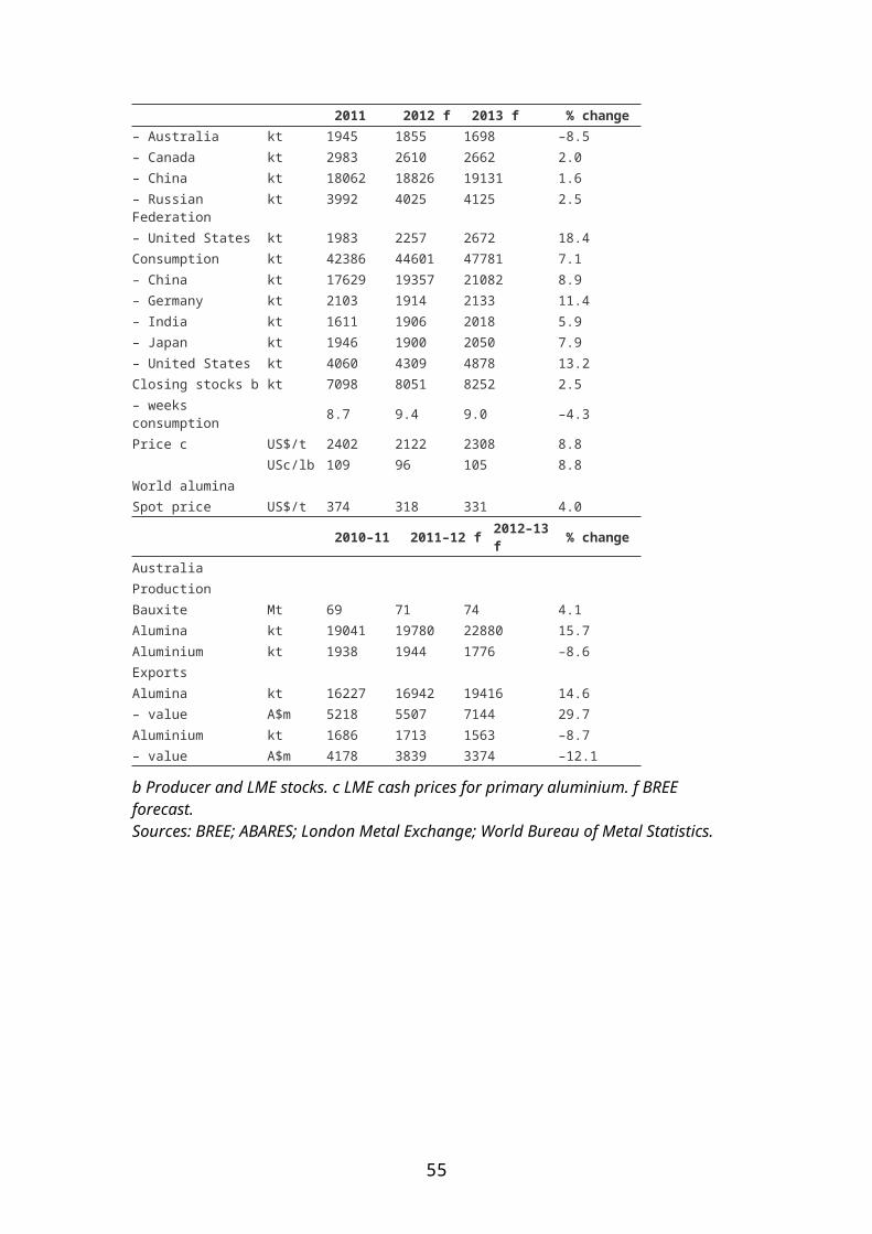
Figure 1: Population growth and number of households


Over the same period, the average living area per person has increased steadily at an average annual rate of 2 per cent, while the number of people per household has decreased gradually at an average rate of 0.5 per cent per year (see Figure 2). During the study period the average living area per person increased substantially, by 45 per cent, to around 64.2 square metres per person in 2009–10.

Figure 2: Average household occupancy and average stock area per person


Although the number of persons per household has decreased, the number of appliances owned by each household has not. The number of appliances in the household sector has increased at an average growth rate of 3.5 per cent per year, much higher than the growth in the Australian population. Appliances with the fastest growing frequency of ownership by households are IT equipment, dishwashers, microwaves, televisions and refrigerators.

Household ownership of IT equipment has increased significantly over the study period (see Figure 3). IT equipment constitutes the fastest growing appliance use in households, with an average annual growth rate of 17.7 per cent (see Figure 4). In 2008–09 and 2009–10, energy consumption of IT equipment accounted for 16 per cent and 16.4 per cent, respectively, of the total energy consumption of household appliances (see Figure 5).

Over the study period, ownership of refrigerators and televisions only increased at an average annual rate of 0.6 per cent and 0.8 per cent, respectively. Nevertheless, they still accounted for a large proportion of household appliance energy consumption. In 2009–10, refrigerators accounted for the largest share of total energy consumption of household appliances at 34 per cent, followed by televisions at 25 per cent.

Figure 3: Household appliance ownership


Figure 4: Annual average growth rate of household ownership of major appliances


55

Figure 5: Shares in total energy consumption of major household appliances in 2009–10


Observed trends in energy consumption of household appliances in Australia

Figure 6 presents the changes in energy consumption of major appliances. From 1989–90 to 2009–10 energy consumption of major appliances increased continually from 37 petajoules to 67 petajoules, or at an average growth rate of 3 per cent per year.

Figure 6: Energy consumption of major appliances


Figure 7 shows the composition of and growth in energy consumption by household appliance. Based on Department of the Environment, Water, Heritage and the Arts (DEWHA 2008) and BREE data of historical and projected energy consumption, it is estimated that refrigerators dominated appliance energy consumption, and contributed to 56 per cent and 34 per cent of overall household appliance energy consumption in 2008–09 and 2009–10, respectively. However, energy consumption for refrigerators only increased by an average of 0.3 per cent per year over the study period.

Information and technology (IT) equipment—a component of household appliances—accounted for 16 per cent of total energy use in households, but at an average annual growth rate of 27 per cent, this was the fastest growing energy use in the residential sector.

Figure 7: Energy consumption of major appliances


Figure 8 shows the decomposition of the change in energy consumption of major household appliances. During the study period, energy consumption of appliances increased by 30.1 petajoules. The activity effect alone resulted in energy consumption increasing by 23 petajoules as a result of an increase in both the number of households and the average units of appliances used per household.

Figure 8: Decomposition of change in energy consumption of major appliances


56

The structural effect represents a shift in the relative use of different appliances. A negative structural effect implies there has been a shift toward less energy intensive appliances by households, such as IT equipment. Between 1989–90 and 2009–10 the structural change effect led to a decrease in energy consumption of appliances by 4.1 petajoules.

The efficiency effect of appliances led to an increase in energy consumption of appliances by 11.2 petajoules. An increase in energy intensity for some end uses, however, does not necessarily indicate lower energy efficiency of these appliances. This is because over the study period energy intensity use per unit of clothes washers, microwaves, IT equipment and televisions increased due to a growing trend of high technology televisions (such as plasma and LCD televisions), larger screen sizes, and larger size with higher level of energy consumption for clothes washers, microwaves and IT equipment.

Trends in energy intensity indicators

Overall, energy intensity of appliances decreased slightly at an average growth rate of 0.4 per cent per year. This is primarily attributed to decreased energy intensity in the appliance group that includes clothes dryers, dishwashers, refrigerators and freezers (see Figure 9), which partly offset increasing energy intensity in the appliance group that includes clothes washers, microwaves, IT equipment and televisions (see Figure 10).

Energy intensity of the appliance group that includes clothes dryers, dishwashers, refrigerators and freezers has fallen over the study period (see Figure 9). The largest declines in energy intensity were in dishwashers and refrigerators, which have fallen by 2.1 per cent and 2 per cent, respectively. Energy consumption of this group of appliances grew at a slower rate than the increasing energy intensity group of clothes washers, microwaves, IT equipment and televisions.

Figure 9: Decreasing energy intensity group of appliances


Energy intensity of the appliance group that includes clothes washers, microwaves, IT equipment and televisions has generally increased over the study period (see Figure 10). This group includes the fastest growing energy users of household appliances over this period. For instance, energy intensity of IT equipment has steadily increased during the study period, at an average rate of 6.4 per cent per year. This may be attributed to significant increases in its energy consumption, which grew at an average rate of 27 per cent per year—the fastest among other household appliances—while the stock owned per household also increased, but at a lower average growth rate of 20 per cent per year.

57

Figure 10: Increasing energy intensity group of appliances


Figure 11 presents trends in energy intensity and the yearly change in energy consumption in major household appliances as a whole. Energy intensity of major household appliances has declined consistently over the period 1989–90 to 2005–06; and has remained relatively stable between 2005–06 and 2006–07 before increasing during the period 2007–08 to 2009–10.

Figure 11: Trends in energy intensity and yearly change in energy consumption of major household appliances


Figure 12 shows the change in energy consumption as a result of the efficiency effect for each year over the study period. The efficiency effect has resulted from increases in energy consumption of household appliances over this period. The exception was in 2004–05 and 2005–06 when energy savings of 0.2 petajoules and 0.1 petajoules, respectively, were achieved. This suggests that the efficiency effect can be an important factor that contributes to savings in energy consumption.

Figure 12: Yearly energy consumption due to the efficiency effect of major appliances


Concluding remarks

Energy intensity of major household appliances decreased at an average annual rate of 0.4 per cent over the period 1989–90 to 2009–10. This is attributed to a shift toward the use of less energy intensive appliances by households. A change in Australian household living standards also contributed to the change in the composition of household energy consumption over the same period. The findings highlight the potential importance of energy efficiency in reducing household energy consumption.

58

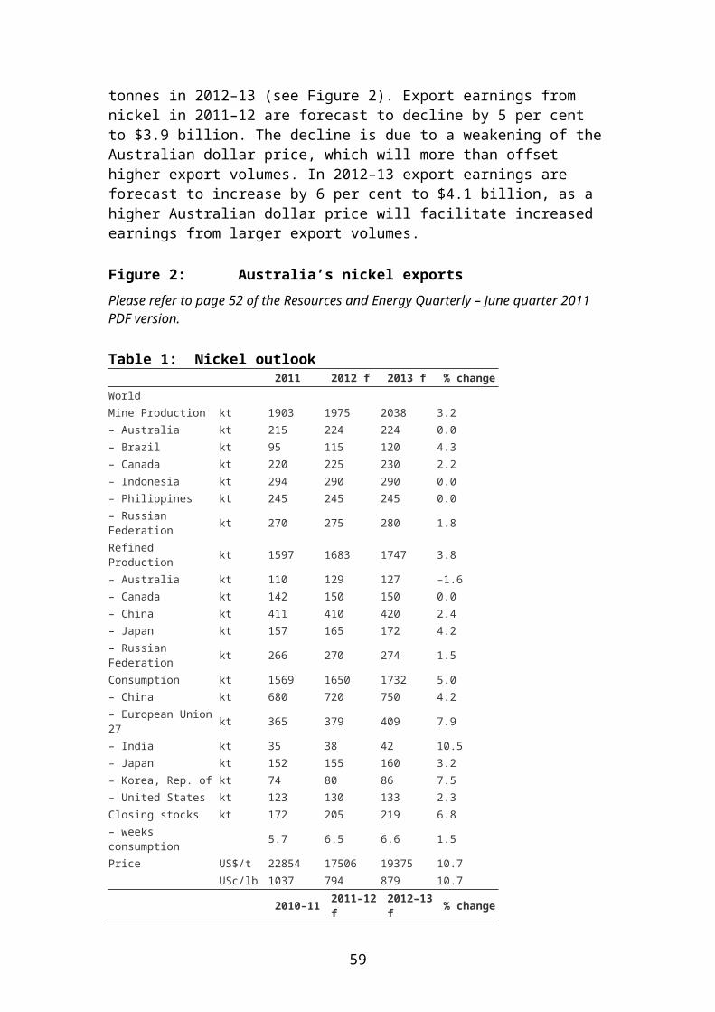
Appendix: Decomposition method of energy consumption

This analysis applies a similar approach used in the report by Sandu and Petchey (2009) and Che and Pham (2012) for energy consumption decomposition analysis (see Ang and Liu 2001 and Ang et al. 2003). Changes in energy use over the study period are separated into three components that affect energy consumption: the activity effect, the structural effect, and the efficiency effect.

The activity effect of an appliance refers to the changes in energy consumption that arise solely from changes in the number of appliances owned by households. The change in energy consumption associated with changes in the composition of household appliance ownership is referred to as the structural effect. The structural effect captures changes in energy consumption when the composition of appliances with different energy intensities grows or declines at different rates, after adjusting for growth in overall activity.

The change in energy consumption associated with the change in the energy intensity of each sector is referred to as the efficiency effect. This measure provides a useful indicator of energy efficiency. However, it is not equal to energy efficiency in the strict engineering sense unless the analysis is undertaken at the most disaggregated level of appliances.

Energy consumption E for household’s appliance category with n appliances can be expressed as:

E = Σni A (Ai / A) (Ei / Ai) (1)

where A is the total activity for household’s appliance, Ai is the activity of an ith appliance and Ei is the energy consumption of the ith appliance. The second term on the right-hand side gives the share of the appliance’s activity of the total activity and the third term gives the energy intensity of the ith appliance. By defining Si = Ai / A and Ii = Ei / Ai, equation (1) can be rewritten as:

E = A Σni Si Ii (2)

The additive type of the log-mean divisia index method (LMDI) decomposition method allows us to express a given change in energy consumption of the ith appliance as the sum of a change in activity (activity effect), a change because of shifts in structure (structural effect) and a change because of changes in energy intensity (efficiency effect):

ΔEi = Ei,T – Ei,O = ωi ln(Ai,T / Ai,O) + ωi ln(Si,T / Si,O) + ωi ln(Ii,T / Ii,O) (3)

where the subscripts 0 and T refer to the value of the variables at the start and end of the interval of interest. The variable ωi is the logarithmic mean of energy consumption across the start and end periods and is defined as:

ωi = (Ei,T – Ei,O) / (lnEi,T – lnEi,O) (4)

59

Similarly, the multiplicative type of the LMDI decomposition method allows us to express a given change in energy consumption of the ith appliance as the product of an activity effect, a structural effect and an efficiency effect:

ΔEi = Ei,T / Ei,O = exp[ψi ln(Ai,T / Ai,O)] x exp[ψi ln(Si,T / Si,O)] x exp[ψi ln(Ii,T / Ii,O)] (5)

Here, the variable ψi is the logarithmic mean of energy consumption across the start 0 and end T periods and is defined as:

ψi = [(Ei,T – Ei,O) / (lnEi,T – lnEi,O)] / [(ET – EO) / (lnET – lnEO)] (6)

References

Ang, B. W., and Liu, F. L., 2001, ‘A new energy decomposition method: perfect in decomposition and consistent in aggregation,’ Energy Policy, vol. 26, pp. 537–548.

Ang, B. W., Liu, F. L., and Chew, E. P., 2003, ‘Perfect decomposition techniques in energy and environmental analysis,’ Energy Policy, vol. 31, pp. 1561–1566.

Australian Bureau of Statistics (ABS) 2011, Australian Demographic Statistics, June 2011, catalogue no. 3101.0, Canberra, December.

Che, N., and Pham, P., 2012, Economic Analysis of End-use Energy Intensity in Australia, Bureau of Resources and Energy Economics, Canberra, May.

Department of Environment, Water, Heritage and the Arts (DEWHA) 2008, Energy use in the Australian residential sector 1986–2020, prepared by Energy Efficient Strategies for DEWHA.

Sandu, S., and Petchey, R., 2009, End use energy intensity in the Australian economy, ABARE research report 09.17, Canberra, November.

60

A short background of the Australian coal industry

Alan Copeland and Rubhen Jeya

Australia is the world’s fourth largest black coal (thermal and metallurgical coal) producer and the world's largest coal exporter. Global and Australian trade has been increasing significantly over the past five years, underpinned by strong import demand from Asia, particularly the Republic of Korea, China and India.

The Australian coal industry makes an important contribution to the Australian economy with exports valued at around $47 billion in 2011. This is equivalent to around 25 per cent of Australia’s resource and energy exports and 15 per cent of Australia’s total goods and services exports. This review focuses on recent developments in Australia's coal industry and the outlook for the next five years.

Reserves

Australia's coal industry is based on large, low cost and high quality reserves. Australia's economically demonstrated coal resources (EDR) as at December 2010 were estimated to be around 42 billion tonnes. In terms of current levels of extraction, this is equivalent to over 90 years production. Despite increases in production over the past five years, Australia's coal reserves to production ratio has remained around 90 years. Almost all of Australia's EDR of black coal are located in Queensland and New South Wales, and vast majority of Australia's coal production and exports originate in these two states.

Coal reserves in the state of Queensland consist of thermal and metallurgical coal. Coal reserves are located in three basins: Bowen, Surat and Galilee. The Bowen Basin is located around 100–250 kilometres inland from the central Queensland coast. The Galilee Basin is located west of the Bowen Basin, while the Surat Basin is located to the south.

The vast majority of Queensland’s thermal coal production and all of its metallurgical coal production occurs in the Bowen Basin. Although there are substantial reserves in the Galilee and Surat Basins, they are as yet untapped. It is possible that production and exports from the Galilee and Surat Basins may occur within the next decade because a number of projects have government approvals and are at an advanced stage of feasibility planning.

Recoverable black coal in New South Wales consists primarily of thermal and semi-soft metallurgical coal. These are located predominantly in the Sydney-Gunnedah basin that extends from south of Sydney through the Hunter Valley and into the north-west of the state near Gunnedah and Narrabri.

The views expressed in this review are those of the authors alone and are not necessarily those of the Bureau of Resources and Energy Economics nor the Department of Resources, Energy and Tourism.

61

Production and exports

In 2011, Australia's coal production was around 400 million tonnes, having increased by an average of 5 per cent a year since 2001. Around 80 per cent of Australia's coal production is exported, with the majority of the remaining production consumed in the electricity generation sector.

The Australian coal industry comprises a diverse range of both publicly listed and privately owned companies. In addition there are a number of locally based companies and those that are headquartered internationally, including Japan, China, India, Thailand and the US. Major coal producers in Australia include BHP Billiton, Rio Tinto, Xstrata, Peabody Energy, Anglo American and Yancoal.

Australia’s coal exports in 2011 were around 281 million tonnes, equivalent to a quarter of world coal trade. Of the 281 million tonnes exported in 2011, 133 million tonnes were metallurgical coal and the remaining 148 million tonnes were thermal coal. Australia's metallurgical coal exports in 2011 were around 10 per cent lower than in 2010, which was a result of heavy rain and flooding across the Bowen Basin in January 2011. The flooding was so significant that many mines still had water in their pits almost 12 months later.

Australia has diverse export markets with the largest being Japan, which accounted for 35 per cent of Australia's exports. Other important markets include the Republic of Korea, China, India and Europe.

Figure 1: Australia’s market share of world exports


Between 2006 and 2011, Australia’s coal exports grew substantially, increasing at an average annual rate of around 4 per cent a year. The increases in Australia's export volumes have been supported by the construction of a number of new mines in the Hunter Valley and the Bowen Basin, and the expansion of port facilities at Newcastle in New South Wales, and Gladstone, Hay Point, Dalrymple Bay and Abbot Point in Queensland.

Recently, Australia’s exports to Asia have increased while volumes into Europe have declined. The changes in Australia’s export markets reflect developments on both the demand and supply side. Asia’s imports of coal have increased by 11 per cent a year over the five years to 2011 to around 750 million tonnes. This increase has been underpinned by growth in imports into China, the Republic of Korea and India.

In China and India, rapid expansion of coal-fired electricity generation and steel production has resulted in domestic coal demand increasing at a rate faster than domestic production. The gap between domestic consumption and production has led to increased imports. In the Republic of Korea, a rapid expansion of coal-fired

62

electricity generation between 2007 and 2009 increased coal demand which was sourced exclusively from imports.

China’s coal exports in 2006 were around 63 million tonnes. By 2011, this had fallen to around 15 million tonnes. The decrease in China’s exports has created an opportunity for other suppliers to raise their exports to Japan and the Republic of Korea, where the majority of China’s coal was shipped to previously. For instance, in 2006 around 11 per cent (19.4 million tonnes) of Japan’s coal imports were sourced from China. By 2011, Japan imported around 3 per cent (7 million tonnes) from China. Producers in Australia and Indonesia have been the main beneficiaries of the decrease in China’s coal exports.

The decrease in Australia’s coal exports to Europe is attributable to two factors. Firstly, European Union (EU) imports of coal have decreased by 4 per cent between 2006 and 2011. Secondly, growth in coal production in Colombia and the Russian Federation has enabled these countries to increase exports, much of which has been exported to the EU. Given the relative proximity to the EU, these two exporting countries have a significant freight cost advantage over producers in Australia and, hence, have been able to increase their share of European imports.

The outlook for Australia’s coal exports over the period 2012 to 2017 is positive based on forecast increases in demand for imports from Asia. Over this period there is expected to be strong increases in imports from India, China, the Republic of Korea and Thailand. Australia’s coal exports are forecast to reach 490 million tonnes in 2017 as Australian coal producers invest in new mine and infrastructure capacity to take advantage of the expected increase in import demand.

The current level of investment in Australian coal mines and infrastructure capacity is substantial. In BREE’s Mining Industry Major Projects—April 2012 publication, there were 21 coal mine projects under construction with a combined value of $17.3 billion. All of these mines are scheduled to be in operation by 2015 and will add around 70 million tonnes a year of production capacity. Of these 21 projects, 11 are located in Queensland, while the other 10 are in New South Wales.

Table 1: Coal projects under constructionNSW

Project OwnerExpected startup New capacity

Capital expenditure*

Austar underground (stage 3)

Yancoal Australia 2014 2 Mt ROM coking $250m

Bengalla expansion (stage 1)

Wesfarmers / Rio Tinto

mid 2012 1.5 Mt ROM US$184m (A$180m)

Boggabri opencut Idemitsu Kosan 2014 3.3 Mt thermal $400m

Hunter Valley Operations Expansion

Rio Tinto / Mitsubishi 2012 6 Mt thermal and semi soft coking

US$260m (A$255m)

Metropolitan longwall Peabody Energy 2013 1 Mt hard coking US$70m (A$69m)

Mount Arthur 0(RX1) BHP Billiton 2013 4 Mt thermal (ROM) $US400m (A$392m)

63

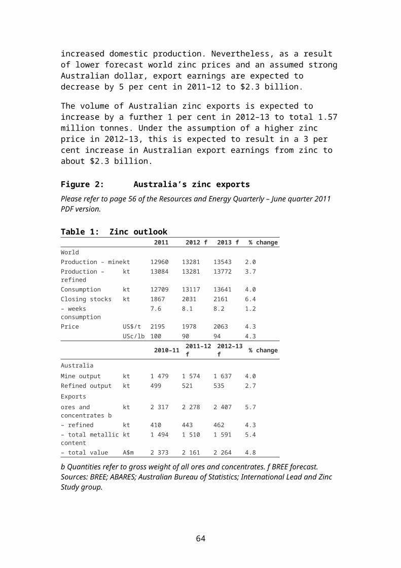
NSW



Narrabri Coal Project (stage 2)

Whitehaven 2012 4.5 Mt thermal $300m

NRE No. 1 Colliery (preliminary works project)

Gujarat NRE Coking Coal

2015 nil (mine upgrade) $122m

Ravensworth North Xstrata 2013 8 Mt thermal and semi soft

US$1.4b (A$1.37b)

Ulan West Xstrata 2014 7 Mt thermal US$1.1b (A$1.08b)

QLD



Broadmeadow (mine life extension)

BHP Billiton Mitsubishi Alliance (BMA)

2013 0.4 Mt coking US$900m (A$882m)

Burton Peabody Energy late 2012 2-3 Mt hard coking na

Caval Ridge / Peak Downs expansion

BHP Billiton Mitsubishi Alliance (BMA)

2014 8 Mt coking US$4.2b (A$4.1b)

Curragh Mine Wesfarmers mid 2012 increase to 8.5 Mt $286m

Daunia BHP Billiton Mitsubishi Alliance (BMA)

2013 4.5 Mt coking US$1.6b (A$1.55b) excl. pre FID funding

Eagle Downs (Peak Downs East underground)

Aquila Resources / Vale

2016 4.5 Mt coking $1.25b

Ensham bord and pillar underground mine

Ensham Resources mid 2012 1.7 Mt thermal $166m

Grosvenor underground Anglo Coal Australia 2013 5 Mt hard coking US$1.7b (A$1.66b)

Kestrel Rio Tinto 2013 1.3 Mt coking US$2b (A$1.96b)

Lake Vermont Jellinbah Resources 2013 4 Mt $200m

Millennium expansion Peabody Energy 2013 1-2 Mt coking US$275m (A$270m)

Source: BREE Mining Industry Major Projects—April 2012.* Total capital expenditure as reported by the company in current dollars. Includes development, plant and equipment costs.

In Queensland, the majority of coal production capacity under construction is hard coking coal. The four largest projects, in terms of production capacity, are BHP Billiton’s Caval Ridge (annual capacity of 8 million tonnes) and Daunia (4.5 million tonnes) mines, Anglo Coal’s Grosvenor mine (5 million tonnes) and Vale’s and Aquilla’s Eagle Downs mine (4.5 million tonnes). All four of these projects are scheduled for completion by 2015. While all of these projects are metallurgical coal mines located in the Bowen Basin, there are a number of thermal coal projects that are going through planning and approval processes that could result in production commencing the Surat and Galilee Basins.

64

The Surat and Galilee Basins have significant reserves of thermal coal and can support large-scale mine developments. Any development of mines in the Surat and Galilee Basin, however, would need to be accompanied by rail connections to existing rail networks (in the case of the Surat Basin) or ports (Galilee Basin). Significant production and exports from the Surat and Galilee Basins are not anticipated until at least the end of this decade.

Of the 10 coal projects under construction in New South Wales, the vast majority will support increased thermal coal production. In terms of production capacity, the four largest projects under construction are Xstrata’s Ravensworth (8 million tonnes of annual capacity) and Ulan West (7 million tonnes) mines, Rio Tinto’s Hunter Valley Operations expansion (6 million tonnes) and Whitehaven’s Narrabri Longwall project (4.5 million tonnes). All four of these projects are scheduled for completion by 2014.

To support increases in Australia’s coal exports, there are 11 coal-related infrastructure projects under construction including six rail expansions and five port expansions. In New South Wales, coal port capacity will be increased by 48 million tonnes following the completion of expansions to the Kooragang Island Coal Terminal and the Newcastle Coal Infrastructure terminal. When the projects are complete, the Port of Newcastle will have a coal handling capacity of 211 million tonnes a year. In Queensland, there are two coal port projects under construction: the first stage of the Wiggins Island Coal Terminal near Gladstone and an expansion and refurbishment of the Hay Point Coal Terminal near Mackay. Both projects are scheduled for completion in 2014 and have a combined coal handling capacity of 38 million tonnes a year. The increases in port capacity in both New South Wales and Queensland are also supported by a number of projects to increase rail capacity.

Beyond infrastructure capacity under construction, there are a number of projects which are being progressed through planning and approvals stages that could increase Australia’s export capacity in the second half of this decade and beyond. These include the T4 project at Newcastle, the second and third stages of Wiggins Island and new coal terminals at Abbot Point. Increased capacity at Wiggins Island could support coal exports from the Surat Basin, while coal from the Galilee Basin could be exported through Abbot Point.

While Australia’s coal industry has grown significantly over the past five years, and will continue to grow over the next five years, it faces some challenges. Australia will have increased competition in export markets from existing exporters (Indonesia, Colombia and North America) and from emerging exporters (Mongolia and Mozambique). Coal production costs are also increasing associated with higher costs for project capital, labour, transportation, equipment and consumables. Australian coal producers will need to manage these costs while facing the challenges of a decline in coal prices expected over the next five years (BREE 2012).

65

Resourcesand Energy

QuarterlyStatistical tables

66

Contribution to GDP


Principle markets for Australian imports in 2010–11 dollars


Principle markets for Australian exports in 2010–11 dollars


Resources and energy sector indicators, Australia


Principle markets for Australian resources and energy exports


Resources and energy prices, ended March Quarter 2012

Please refer to pages 92–93 of the Resources and Energy Quarterly – June quarter 2011 PDF version.

Table 1: Annual exports summary, Australia, Balance of payments basis2007–08 2008–09 2009–10 2010–11 2011–12 f

At current prices $m $m $m $m $mMineral resources– Coal, coke and briquettes 24 603 54 954 36 777 44 101 48 016 48 756

– Other mineral fuels 18 889 20 706 18 964 23 594 26 492 31 305– Metalliferous ores and other minerals 41 930 52 733 54 082 79 814 85 618 91 395

– Gold 12 272 17 508 14 300 14 256 16 952 21 702– Other metals bs 18 211 14 358 14 031 15 963 14 574 14 415– Total s 115 904 160 259 138 154 177 729 191 652 207 573Total commodities sector s 145 875 194 176 168 630 212 095 227 688 242 871

Other merchandise s 37 047 37 447 33 121 34 884 na naTotal merchandise s 182 922 231 623 201 751 246 979 na naServices 50 891 52 948 52 011 50 859 na naTotal goods and services 233 813 284 571 253 762 297 838 na na

Chain volume measures cMineral resources– Coal, coke and 29 585 30 951 36 777 35 279 36 527 40 145

67

2007–08 2008–09 2009–10 2010–11 2011–12 fbriquettes– Other mineral fuels 16 568 17 523 18 964 20 027 19 260 23 196– Metalliferous ores and other minerals 47 367 46 991 53 994 55 602 61 631 67 215

– Gold 16 500 18 348 14 300 12 767 13 001 15 546– Other metals bs 13 907 14 358 13 668 14 356 15 174 15 109– Total s 123 928 128 171 137 703 138 031 145 592 161 212Total commodities sector s 153 155 159 801 169 473 170 983 184 271 na

Other merchandise s 31 088 28 175 32 277 33 855 na naTotal merchandise s 184 243 187 976 201 750 204 838 na naServices 53 651 54 023 52 011 49 842 na naTotal goods and services 236 965 241 051 253 761 254 680 na na

a Includes diamonds, which are not included in the balance of payments item by the ABS. b Includes BREE estimates for steel and nickel, which are retained as confidential by the ABS. c For a description of chain volume measures, see ABS, Introduction of chain volume measures, in the Australian National Accounts, cat. no. 5248.0, Canberra. Reference year is 2009–10. s BREE estimate. f BREE forecast. na Not available.Sources: BREE; ABARES; Australian Bureau of Statistics, Balance of Payments and International Investment Position, Australia, cat. no. 5302.0, Canberra.

Table 2: Unit export returnsAnnual indexes a 2006–

072007–08

2008–09

2009–10

2010–11 s

2011–12 f

2012–13 f

Metals and other minerals 201.5 199.8 225.8 210.3 281.2 270.6 271.1

Energy 206.6 235.8 398.3 258.9 317.0 345.7 329.2Total resources and energy 204.3 214.3 290.6 229.3 295.5 299.2 293.6

a In Australian dollars. Base: 1989–90 = 100. s BREE estimate. f BREE forecast.Sources: BREE; ABARES.

Table 3: Contribution to exports by sector, balance of payments basisPlease refer to page 96 of the Resources and Energy Quarterly – December quarter 2011 PDF version.

Table 4: Industry gross value added a bunit 2006–07 2007–08 2008–09 2009–10 2010–11

Agriculture, forestry and fishing $m 23138 24742 29108 28765 29796Mining– mining (excludes services to mining) $m 78935 79923 82209 87796 88243

– exploration and mining support services $m 7783 8632 8656 8309 9171

– total $m 86446 88193 90508 96106 97447Manufacturing– food, beverage and tobacco product $m 23160 23127 22404 23953 23576

– textile, clothing and other manufacturing $m 9262 9695 8688 7150 6647

– wood and paper products $m 8400 8071 7457 7736 7567– printing and recorded media $m 5048 5174 4268 4088 4101

68

unit 2006–07 2007–08 2008–09 2009–10 2010–11

– petroleum, coal, chemical, etc, product $m 18652 19114 17200 17807 17907

– non-metallic mineral products $m 5673 5926 5890 5783 5608– metal products $m 20408 22718 21992 21310 21515– machinery and equipment $m 19257 19884 18760 19881 19552– total $m 108703 113062 106363 107707 106476Construction $m 86469 92517 95291 95804 101794Electricity, gas, water and waste services $m 26798 26866 27894 28623 28893

Taxes less subsidies on products $m 89888 91667 90826 90334 91073Statistical discrepancy $m 0 0 –1 0 –3577Gross domestic product $m 1201562 1246899 1263934 1293380 1317914

a Chain volume measures, reference year is 2009–10. b ANZSIC 2006.Source: Australian Bureau of Statistics, Australian National Accounts: National Income, Expenditure and Product, cat. no. 5206.0, Canberra.

Table 5: Volume of production indexes2007–08 2008–09 2009–10 2010–11 2011–12 f 2012–13 f

Mine aEnergy minerals 116.9 122.6 125.5 121.8 127.0 136.4Metals and other minerals 124.1 119.6 123.2 138.9 144.2 152.0

Total minerals 120.4 121.1 124.4 130.3 135.6 144.1

a Uranium is included with energy. s BREE estimate. f BREE forecast.Note: The indexes for the different groups of commodities are calculated on a chained weight basis using Fisher’s ideal index with a reference year of 1997–98 = 100.Sources: BREE; ABARES; Australian Bureau of Statistics.

Table 6: Employment a b2005–06

2006–07

2007–08

2008–09

2009–10

2010–11

’000 ’000 ’000 ’000 ’000 ’000Agriculture, forestry and fishing 348 352 355 362 369 351Mining– coal 29 27 26 35 41 48– oil and gas extraction 9 10 11 15 15 13– metal ore 42 46 47 49 52 69– other mining (including services) 49 53 62 72 66 75– total 129 136 146 170 173 205Manufacturing – food, beverages and tobacco 205 215 230 226 228 229– textiles, clothing, footwear and leather 56 51 50 48 46 45

– wood and paper product 77 77 70 67 64 57– printing, publishing and recorded media 52 51 54 51 52 56

– petroleum, coal and chemical product 88 92 98 90 88 85

– non-metallic mineral product 38 36 42 40 37 37– metal product 161 161 159 157 147 147– other manufacturing 347 342 360 348 343 336– total 1025 1025 1063 1028 1006 992

69

2005–06

2006–07

2007–08

2008–09

2009–10

2010–11

Other industries 8587 8876 9144 9332 9479 9806Total 10089 10388 10708 10892 11027 11355

a Average employment over four quarters. b ANZSIC 2006. Caution should be used when using employment statistics at the ANZSIC subdivision and group levels due to estimates that may be subject to sampling variability and standard errors too high for most practical purposes.Source: Australian Bureau of Statistics, Labour Force, Australia, cat. no. 6291.0, Canberra.

Table 7: Business income2006–07 2007–08 2008–09 2009–10 2010–11

Company profits in selected industries a $m $m $m $m $m

Mining 40311 40184 67402 49889 76563Manufacturing– food, beverages and tobacco 4532 5757 6166 8168 na– textiles, clothing, footwear and leather 548 501 245 409 na

– wood and paper product 1085 1184 667 615 na– printing, publishing and recorded media 578 620 170 439 na

– petroleum, coal and chemical product 3859 6192 2159 3676 na

– non-metallic mineral product 1108 1359 978 1155 na– metal product 10004 7924 3781 2662 na– machinery and equipment 1640 1937 2695 3383 na– other manufacturing 762 851 637 712 na– total 24116 26325 17498 21219 20344Other industries (including services)88856 99836 73102 98834 103016Total (including services) 153272 166325 157986 169932 199645

a Company profits before income tax, based on ANZSIC 2006.Sources: BREE; Australian Bureau of Statistics, Australian National Accounts: National Income, Expenditure and Product, cat. no. 5206.0, Canberra; Australian Bureau of Statistics, Company Profits, Australia, cat. no. 5651.0, Canberra; Australian Bureau of Statistics, Business Indicators, Australia, cat. no. 5676.0, Canberra; Australian Bureau of Statistics, Australian Industry, cat. no. 8155.0, Canberra.

Table 8: All banks lending to business a2009–10 2010–11 2011-12Mar Jun Sep Dec Mar Jun Sep Dec$b $b $b $b $b $b $b $b

Agriculture, fishing and forestryMining 57.8 59.1 58.7 58.8 58.6 60.4 60.5 60.1Manufacturing 14.1 12.1 11.3 11.2 11.0 12.1 13.2 14.1Construction 40.8 39.2 38.6 38.2 40.1 39.9 42.1 42.0Wholesale, retail trade, transport and storage 29.4 28.2 28.3 28.2 28.7 28.4 27.7 26.8

Finance and insuranceOther 91.9 90.5 89.3 92.0 92.6 92.5 95.2 96.8Total 128.7 133.0 132.0 125.0 121.2 114.8 120.1 120.1

70

a Includes variable and fixed interest rate loans outstanding plus bank bills outstanding.Source: Reserve Bank of Australia, Bank Lending to Business – Selected Statistics, Bulletin Statistical Table D8.

Table 9: Capital expenditure of private enterprises2006–07 2007–08 2008–09 2009–10 2010–11

At current prices $m $m $m $m $mGross fixed capital formation aAll sectors 299101 336357 351112 356037 370295New capital expenditureMining b 23621 29201 37977 35185 46847Manufacturingfood, beverages and tobacco 2256 2596 2492 2566 2882textiles, clothing, footwear and leather 139 112 118 140 70

wood and paper product 759 928 897 719 610printing, publishing and recorded media 353 396 450 452 187

petroleum, coal and chemical product 1767 2126 2239 2207 2320

non-metallic mineral product 467 474 609 731 806metal product 4761 4137 4608 3689 4017machinery and equipment 1436 1110 1160 1112 1340other manufacturing 58 164 108 126 111total 12106 12340 12682 11743 12343Total surveyed industries 87475 96833 113201 107104 119341Chain volume measures cGross fixed capital formation aAll sectors 313198 343309 348084 356036 369742New capital expenditureMining 25463 30546 37627 35184 46919Manufacturing 12663 13032 12627 11743 12713Other selected industries 49861 54942 60515 60178 62076Total surveyed industries 88109 98524 110727 107105 121709

a Estimates taken from ABS national accounts, which include taxation-based statistics. b ANZSIC 2006 Division B. c Reference year is 2009–10.Sources: BREE; ABARES; Australian Bureau of Statistics, Australian National Accounts: National Income, Expenditure and Product, cat. no. 5206.0, Canberra; Australian Bureau of Statistics, Private New Capital Expenditure and Expected Expenditure, Australia, cat. no. 5625.0, Canberra.

Table 10: Private mineral exploration expenditure2005–06

2006–07

2007–08

2008–09

2009–10

2010–11

At current prices $m $m $m $m $m $m

EnergyPetroleum – onshore 355.8 498.2 493.8 492.3 748.6 756.5– offshore 906.1 1727.3 2 541.1 3 318.4 2 745.5 2 558.9total 1 261.9 2 225.5 3 034.9 3 810.7 3 494.1 3 315.4Coal 166.4 193.2 234.8 297.3 321.2 519.7Uranium 56.1 114.1 231.5 185.2 169.1 213.9Total 1 484.4 2 532.8 3 501.2 4 293.2 3 984.4 4 049.0

71

2005–06

2006–07

2007–08

2008–09

2009–10

2010–11

Metals and other minerals aGold 399.6 455.9 592.6 438.0 575.4 652.2Iron ore 161.3 285.4 449.8 588.7 524.1 665.0Base metals, silver and cobalt b 356.7 555.0 783.2 519.1 457.2 669.5

Mineral sands 29.2 37.3 37.0 30.6 na naDiamonds 22.6 26.9 21.7 10.0 na naOther 48.8 46.8 110.8 154.3 147.2 196.2Total metals and other minerals a 1 018.2 1 407.3 1 995.1 1 740.7 1 742.3 2 217.7

Total expenditure 2 502.6 3 940.1 5 496.3 6 033.9 5 726.7 6 266.7

a Uranium is included with energy. b Base metals include copper, lead, nickel and zinc. s BREE estimate.Sources: BREE; Australian Bureau of Statistics, Mineral and Petroleum Exploration, Australia, cat. no. 8412.0, Canberra.

Table 11: Annual world indicator prices of selected commoditiesunit 2007–

082008–09

2009–10

2010–11 2011–12 f 2012–13

fEnergyCrude oilDubai US$/bbl 90.4 68.5 74.2 92.2 104.1 108.7West Texas Intermediate US$/bbl 96.8 70.3 75.2 89.3 95.0 96.3Brent dated US$/bbl 95.2 68.8 74.5 96.0 111.7 110.9Uranium (U3O8) a US$/lb 80.75 51.25 43.81 57.13 51.58 55.04Minerals and metals bAluminium US$/t 2667 1868 2016 2383 2203 2170Copper US$/t 7785 4919 6691 8671 8227 7671Gold d US$/oz 823 874 1092 1372 1673 1706Iron ore (negotiated) d USc/dmtu 80 145 97 180 230 214Lead US$/t 2904 1459 2093 2392 2185 2185Manganese (negotiated) e US$/mtu 540.9 1340.1 544.9 768.0 544.1 naNickel US$/t 28564 13322 19390 23963 19217 17750Silver USc/oz 1544 1289 1688 2880 3326 3628Tin US$/t 18529 13576 16202 23960 20011 17498Zinc US$/t 2606 1403 2066 2243 2046 2191

a World trade weighted average price compiled by the US Department of Energy. Official sales prices or estimated contract terms for major internationally traded crude oils. b Average of weekly restricted spot prices over the period, published by Ux Consulting. c Average LME spot price unless otherwise stated. d London gold fix, London Bullion Market Association. e Australian hematite fines to Japan (fob) for Japanese Fiscal Year commencing 1 April. BREE Australia–Japan average contract price assessment. g Japanese Fiscal Year commencing 1 April. s BREE estimate. f BREE forecast. na Not available.Sources: BREE; Australian Bureau of Statistics; International Energy Agency; ISTA Mielke and Co.; London Bullion Market Association; The London Metal Exchange Ltd; Reuters Ltd; Ux Consulting Company; Platts Oilgram; US Department of Energy; World Bureau of Metal Statistics.

72

Table 12: World production, consumption and trade for selected commodities a

unit 2008 2009 2010 2011 s 2012 f 2013 fEnergy Crude oilProduction– world b mbd 86.5 85.6 87.2 88.3 90.1 91.5– OPEC c mbd 35.8 34.1 34.6 35.6 36.8 37.9Consumption b mbd 86.2 85.6 88.4 89.2 90.1 91.5Coal Productionhard coal d Mt 5653 5842 6020 6225 6443 nabrown coal Mt 965 913 930 935 954 naExports– metallurgical coal Mt 234 220 273 270 284 292– thermal coal Mt 704 721 794 837 871 919Uranium (U3O8) Production e s kt 53.5 53.3 55.2 56.6 58.2 61.3Consumption kt 76.2 77.2 79.8 73.8 77.3 88.7MetalsBauxite production kt 217469 193038 203460 240587 255102 268695Alumina production kt 77564 73667 81023 89248 91108 95962Aluminiumproduction kt 39669 37197 41911 44624 45554 47981consumption kt 36900 34765 40173 42386 44601 47781closing stocks g kt 4709 6485 6502 7098 8051 8252Iron and steelProduction– iron ore h Mt 1693 1588 1815 2080 2134 2243– pig iron Mt 927 900 1020 1133 1183 1231– crude steel Mt 1330 1220 1415 1511 1573 1634Iron ore trade Mt 889 955 1055 1072 1122 1228GoldMine production t 2429 2611 2741 2818 2907 2977Supply t 4014 4380 4383 4479 4468 4427Fabrication consumption i t 3027 2517 2784 2759 2808 2856

unit 2008 2009 2010 2011 2012Base MetalsCopperproduction j kt 18497 18605 19222 19578 20329 21376consumption kt 18138 18153 19204 19508 20420 21420closing stocks kt 845 1125 1017 957 866 822Leadproduction j kt 9075 9054 9682 10372 10653 11139consumption kt 9072 9069 9683 10216 10556 10865closing stocks kt 307 390 447 623 720 995Nickelproduction j kt 1382 1322 1446 1600 1690 1773consumption kt 1278 1241 1464 1572 1656 1757closing stocks kt 155 234 213 172 207 220Tinproduction j kt 332 333 352 369 369 384consumption kt 337 322 368 375 375 385closing stocks kt 32 46 16 5 45 45Zinc

73

unit 2008 2009 2010 2011 s 2012 f 2013 fproduction j kt 11778 11286 12830 13062 13480 13971consumption kt 11565 10920 12572 12709 13345 13951closing stocks kt 820 1217 1562 1915 2050 2070Mineral SandsProduction– ilmenite k kt 11422 9881 11470 11310 11614 na– titaniferous slag kt 2695 2247 2749 2545 2610 na– rutile concentrate kt 615 572 708 679 639 na– zircon concentrate kt 1282 1067 1338 1442 1376 na

a Some figures are not based on precise or complete analyses. b 1 million litres (1 megalitre) a year equals about 17.2 barrels a day. c Includes OPEC natural gas liquids. d Includes anthracite and bituminous coal, and for the United States, Australia and New Zealand, sub-bituminous coal. e World production data have been revised to exclude reprocessed uranium. g LME and producer stocks. h China’s iron ore production adjusted to world average. i Includes jewellery consumption. j Primary refined metal. k Excludes some small producers and large tonnages produced from ilmenite–magnetite ore in the Commonwealth of Independent States. s BREE estimate. f BREE forecast. na Not available.Sources: BREE; ABARES; Australian Bureau of Statistics; Consolidated Gold Fields; Economic Commission for Europe; Gold Fields Mineral Services; International Atomic Energy Agency; International Energy Agency; International Iron and Steel Institute; International Lead–Zinc Study Group; International Nickel Study Group; ISTA Mielke and Co.; Metallgesellschaft A.G.; UNCTAD Trust Fund on Iron Ore; United Nations; World Bureau of Metal Statistics.

Table 13: Commodity production

unit2007–08 2008–09 2009–10 2010–11 2011–12

f2012–13 f

EnergyCoal– black, saleable Mt 326.2 339.6 362.5 344.8 364.1 s 408.8 s– black, raw Mt 422.8 446.2 466.9 453.4 487.3 s 530.9 s– brown Mt 66.0 68.3 68.8 65.7 na naPetroleum– crude oil and condensate ML 25610 k 26407 k 25583 k 24745 k 22826 k 23034 k– petroleum products a ML 39575 39546 37200 38393 37598 34387Gas b Gm3 41.7 44.5 50.1 53.1 52.1 58.9LPG (naturally occurring) ML 3971 3930 4097 3907 3913 3946Uranium (U3O8) t 10123 10311 7109 7069 7217 7860Metalliferous minerals and metalsAluminium– bauxite Mt 63.5 64.1 67.8 68.5 71.7 73.9– alumina kt 19359 19597 20056 19041 19780 22880– aluminium (ingot metal) kt 1964 1974 1920 1938 1944 1776Copper– mine production d kt 847 890 819 952 971 1113– refined, primary kt 444 499 395 485 484 504Gold– mine production d t 229.7 217.9 239.7 265.4 261.5 282.6– Iron and steel– ore and concentrate e Mt 324.7 353.2 423.4 450.0 508.8 526.6– iron and steel Mt 8.2 5.6 6.9 7.3 5.4 4.9Lead– mine production d kt 641 596 617 697 707 590

74

unit2007–08 2008–09 2009–10 2010–11 2011–12

f2012–13 f

– refined g kt 203 213 189 190 194 181– bullion kt 152 155 148 133 152 150Manganese– ore, metallurgical grade kt 5428 3730 5795 6784 7355 7348– metal content of ore kt 2188 1504 2365 2756 3014 3010Nickel h – mine production d kt 190 185 157 195 226 221– refined, class I s kt 105 95 114 90 106 114– refined, class II i kt 15 15 6 10 15 15– total ore processed j kt 222 213 197 236 272 273Silver– mine production d t 1867 1764 1809 1792 1905 1987– refined t 605 751 701 712 883 948Tin– mine production d t 1767 4045 19829 18410 9202 s 6024– refined t na na na na na 320Titanium– ilmenite concentrate s kt 2205 1932 1398 1275 1298 1295– leucoxene concentrate s kt 153 117 123 200 228 228– rutile concentrate s kt 332 285 361 467 482 520– synthetic rutile s kt 672 732 553 542 519 561– titanium dioxide pigment s kt 201 214 222 204 204 204Zinc– mine production d kt 1571 1411 1362 1479 1574 1637– refined kt 507 506 515 499 521 535Zircon concentrate s kt 563 485 408 674 698 613Other mineralsDiamonds ’000 ct 16528 15169 11138 8027 10168 12160Salt kt 9826 11314 11772 11562 11413 s 11159

a Excludes production from petrochemical plants. b Includes ethane, methane and coal seam gas. c Uranium is included with energy. d Primary production, metal content. e Excludes iron oxide not intended for metal extraction. g Includes lead content of lead alloys from primary sources. h Products with a nickel content of 99 per cent or more. Includes electrolytic nickel, pellets, briquettes and powder. i Products with a nickel content of less than 99 per cent. Includes ferronickel, nickel oxides and oxide sinter. j Includes imported ore for further processing. k Energy Quest. s BREE estimate. f BREE forecast.Sources: BREE; ABARES; Australian Bureau of Statistics; Consolidated Gold Fields; Coal Services Pty Limited; Department of Resources, Energy and Tourism; Energy Quest; International Nickel Study Group; Queensland Government, Department of Natural Resources and Mines.

Table 14: Volume of commodity exportsunit 2007–08 2008–09 2009–10 2010–11 2011–12

f 2012–13 f

Resources and energyResourcesMetalliferous minerals and metals cAluminiumBauxite kt 7917 7470 8023 8595 9977 8894Alumina kt 15739 16395 16653 16227 16942 19416Aluminium (ingot metal) kt 1650 1748 1624 1686 1713 1563

75

unit 2007–08 2008–09 2009–10 2010–11 2011–12 f 2012–13 f

CopperOre and concentrate d kt 1694 1797 1928 1750 1832 2227Refined kt 296 361 271 375 386 365Gold e t 382 437 335 301 331 361Iron and steelIron ore and pellets Mt 294 324 390 407 463 510Iron and steel g kt 2131 1741 1549 1785 1186 1018LeadOres and concentrates kt 308 381 491 494 435 404Refined kt 193 261 186 213 223 178Bullion kt 169 147 151 93 153 150Manganese d kt 5105 3226 5648 6190 6504 6854Nickel es kt 211 194 221 210 240 258TitaniumIlmenite concentrate h kt 894 1538 1763 1804 2045 2035Leucoxene concentrate kt 69 61 18 27 31 31Rutile concentrate kt 399 550 575 491 334 367Synthetic rutile s kt 513 512 513 517 536 462Titanium dioxide pigment kt 175 141 181 195 191 191Refined silver t 335 423 420 198 275 474Tin e t 3079 4159 6031 5431 4838 5704ZincOres and concentrates d kt 2323 2101 2271 2317 2373 2363Refined kt 411 451 425 410 452 462Zircon concentrate i kt 637 685 748 963 846 771Other mineralsDiamonds ’000 ct 16528 16279 10355 9900 11526 12160Salt kt 10686 10978 11185 11162 10884 10773EnergyCrude oil a ML 15975 16588 18064 19638 19167 19389LPG ML 2589 2500 2776 2471 2203 2276LNG bs Mt 14 15 18 20 19 23Petroleum products ML 1807 1164 850 760 877 1117Metallurgical coal Mt 137 125 157 140 142 161Thermal coal Mt 115 136 135 143 159 179Uranium (U3O8) t 10139 10114 7555 6950 s 7217 s 7860 s

a Includes condensate and other refinery feedstock. b 1 million tonnes of LNG equals aprroximately1.31 billion cubic metres of gas. c International ships and aircraft stores. d Uranium is included with energy. e Quantities refer to gross weight of all ores and concentrates. g Quantities refer to total metallic content of all ores, concentrates, intermediate products and refined metal. h Includes all steel items in ABS, Australian Harmonized Export Commodity Classification, ch. 72, ’Iron and steel’, excluding ferrous waste and scrap and ferroalloys. i Excludes leucoxene and synthetic rutile. j Data from 1991–92 refer to standard grade zircon only. s BREE estimate. f BREE forecast.Sources: BREE; ABARES; Australian Bureau of Statistics, International Trade, Australia, cat. no. 5465.0, Canberra; Australian Mining Industry Council; Department of Foreign Affairs and Trade; Department of Resources, Energy and Tourism; International Nickel Study Group.

Table 15: Value of commodity exports (fob)2007–08 2008–

092009–10

2010–11

2011–12 f

2012–13 f

$m $m $m $m $m $m

76

2007–08 2008–09

2009–10

2010–11

2011–12 f

2012–13 f

ResourcesMetalliferous minerals and metalsAluminium Bauxite s 206 192 178 229 280 249Alumina 5809 6015 4969 5218 5507 7144Aluminium (ingot metal) 4967 4724 3838 4178 3839 3374Copper cOre and concentrate 4151 3618 4526 5130 5417 6259Refined 2579 2245 1980 3292 3001 2784Gold c 10903 16146 12996 13016 15558 19722Iron and steelIron ore and pellets 20511 34239 35075 58387 62788 66936Iron and steel 1562 1363 1120 1303 983 789Lead cOres and concentrates 757 645 998 1301 1125 838Refined 674 560 425 511 490 369Bullion 595 432 409 248 490 311ManganeseOres and concentrate s 1532 1406 1395 1407 1176 1229TitaniumIlmenite concentrate d 104 171 197 198 225 224Leucoxene concentrate 23 37 11 17 22 23Rutile concentrate 277 335 382 390 252 270Synthetic rutile s 305 258 269 315 294 252Titanium dioxide pigment 375 396 448 527 594 590Nickel s 5412 2717 3875 4096 3902 4138Refined silver 187 245 254 164 290 521Tin c 42 70 101 126 98 103Zinc cOres and concentrates 2031 935 1237 1479 1357 1387Refined 1319 923 977 893 906 945Zircon concentrate e 421 540 370 532 327 231Total metalliferous minerals and metals 64745 78212 76031 102955 108920 118687

Other mineralsDiamonds s 625 676 471 366 421 467Salt 232 237 247 251 245 242Other 6169 4778 5241 5995 6556 7752Total other minerals 7026 5691 5959 6612 7222 8461Total resources 71771 83903 81990 109567 116142 127147EnergyCrude oil a 10484 8757 9534 11772 12621 12698LPG 1182 1044 1105 1068 1040 1113LNG 5854 10079 7789 10437 11647 12808Bunker fuel b 1457 1537 1315 1508 1672 1857Other petroleum products 1323 788 566 526 601 932Metallurgical coal 16038 36813 24526 29793 31094 30122Thermal coal 8365 17885 11886 13956 17845 17641Uranium (U3O8) 887 990 757 610 s 707 s 777 sTotal energyDerived as sum of above 45591 77892 57478 69670 77227 77947On balance of payments basis (excl. bunker fuel) 43492 75660 55741 67718 75153 75749

Total resources and energy

77

2007–08 2008–09

2009–10

2010–11

2011–12 f

2012–13 f

exports Derived as sum of above 117362 161796 139468 179211 199166 208316On balance of payments g 115904 160259 138154 177703 197494 206459Total agricultural exports At current prices 31340 35905 32082 36079 38017 37286On balance of payments g 29971 33917 30476 34366 35657 35298Total commodity exports hDerived as sum of above 148702 197701 171551 215290 237183 245602On balance of payments g 145875 194176 168630 212069 233151 241757

a Includes condensate and other refinery feedstock. b International ships and aircraft stores. c Value of metals contained in host mine and smelter products are not available separately and are included in the value of the mineral product or metal in which they are exported. d Excludes leucoxene and synthetic rutile; data from 1991–92 refer to bulk ilmenite only. e Data refer to standard grade zircon only. g As derived in table 1. h Sum of resources, energy and agricultural commodity exports. s BREE estimate. f BREE forecast.Sources: BREE; ABARES; Australian Bureau of Statistics, International Trade, Australia, cat. no. 5465.0, Canberra; Department of Resources, Energy and Tourism.

Table 16: Value of imports of selected commodities, Australia

2006–07 2007–08 2008–09 2009–10 2010–11$m $m $m $m $m

Resources and energy– aluminium (ingot metal) 11 10 10 27 18– diamonds 397 444 417 442 397– ferroalloys 116 154 181 118 127– gold (refined and unrefined) 5309 7311 11250 7739 5426– ingot steel 2479 2225 3191 1889 2121– iron ore 338 311 269 259 417– petroleum— crude oil a 13360 17149 14727 15031 19578— natural gas 800 724 2166 1219 1929— petroleum products b 7784 12730 13129 11296 12050– phosphate rock 32 80 193 10 57– phosphates 267 778 549 347 628– silver 98 80 223 107 490– other 707 483 794 1183 859Total resources and energy 31698 42479 47098 39666 44097a Includes condensate and other refinery feedstock. b Includes LPG.Sources: BREE; Australian Bureau of Statistics, International Trade, Australia, cat. no. 5465.0, Canberra.

Table 17: Quarterly commodity production2009–10 2010–11 2011–12Jun Sep Dec Mar Jun Sep Dec Mar p

AluminiumBauxite kt 16541 17504 17398 16431 17189 18008 18349 17844Alumina kt 4950 5061 4843 4471 4666 4726 4864 4866Aluminium (ingot metal) kt 480 488 488 476 486 490 493 481CoalBlack, raw Mt 118 124 113 101 116 125 127 114Black, saleable Mt 90 94 89 77 85 93 93 85

78

2009–10 2010–11 2011–12Jun Sep Dec Mar Jun Sep Dec Mar p

Brown as Mt na 16 16 16 16 na na naCopperMine production bs kt 207 236 244 232 239 235 252 228Blister c kt 104 116 119 108 116 105 112 115Refined s kt 108 120 123 117 125 114 121 124

Diamonds '000 ct 2672 2470 2283 1667 1607 2335 1953 2840

GoldMine production bs t 65 68 68 63 66 65 64 63Refined t 104 79 90 78 75 81 86 77IronIron ore and concentrate kt 105206 109077 115720 104632 120586 127227 135450 126362Iron and steel s kt 1813 1848 1887 1867 1704 1753 1214 1212LeadMine production bs kt 172 186 207 140 164 157 160 195Bullion c kt 38 30 36 27 40 41 31 40Refined kt 50 33 57 49 51 42 45 54Manganese s kt 1355 1798 1698 1448 1840 1909 1766 1871Nickel Mine production bs kt 36 45 49 48 53 53 61 57Intermediate kt 15 14 20 13 14 10 16 12Refined, class 1 kt 23 25 18 23 25 26 23 29Refined, class 2 kt 2 2 3 2 3 4 4 4Petroleum, fieldCrude oil and condensate e ML 7252 7246 6402 5316 5780 5749 5954 5190

LPG (naturally occurring) ML 1025 1122 948 913 924 1033 956 908Gas d Mm3 12376 14207 13117 12265 13513 13193 12297 11577Petroleum, total refinery ML 9039 9736 9527 9483 9646 9318 9647 9520Salt s kt 2936 3091 3091 2885 2494 3067 2957 2544SilverMine production bs t 443 485 491 340 476 428 481 426Refined t 170 136 174 189 212 250 247 168TinMine production bs t 4673 4610 4600 4600 4600 3100 3100 1496Titanium sIlmenite concentrate kt 325 328 326 300 322 326 329 319Leucoxene concentrate kt 37 43 48 53 58 57 57 57Rutile concentrate kt 111 121 112 111 122 127 114 98Synthetic rutile kt 140 139 141 133 129 118 123 105Titanium dioxide pigment kt 51 51 51 51 51 51 51 51Uranium oxide (U3O8) t 1683 2008 2209 1668 1185 2070 2019 1618ZincMine production bs kt 385 368 391 337 384 401 394 389Refined kt 130 124 126 123 125 126 133 131 sZircon concentrate s kt 138 158 156 177 183 211 191 164

a Quarterly data are not available. b Total metallic content of minerals produced. c Metallic content. d Includes methane, ethane and coal seam gas. e Energy Quest. p Preliminary. s BREE estimate. na Not available.Sources: BREE; ABARES; Australian Bureau of Statistics, Canberra; Coal Services Pty Limited; Energy Quest; Queensland Government, Department of Mines and Energy; Department of Resources, Energy and Tourism, Canberra.

79

Table 18: Quarterly commodity exports, by volume2009–10 2010–11 2011–12Jun Sep Dec Mar Jun Sep Dec Mar p

AluminiumBauxite kt 2215 2055 1772 2105 2663 2724 2803 2313Alumina a kt 4293 4264 4141 3728 4094 4054 4103 4396Aluminium (ingot metal) kt 445 445 428 421 392 429 439 422Coal, blackMetallurgical Mt 43.59 39.95 39.98 27.47 33.04 35.33 37.17 34.66Thermal Mt 33.86 39.04 37.57 30.26 36.45 39.66 41.14 36.86Copper bs kt 220 213 235 208 222 219 255 212

Diamonds cs '000 ct 2845 2650 2700 2500 2050 2684 2961 2840

Gold bs t 98.61 68.61 83.17 77.78 71.05 78.07 80.71 86.52IronIron ore and pellets kt 99650 99026 108618 93737 105499 117314 121289 108473Iron and steel s kt 483 415 605 393 371 458 206 263Lead bs kt 185 150 192 158 177 168 189 156

Manganese ore and concentrate kt 1351 906 1761 1681 1841 1787 1604 1419

Nickel ds kt 55 56 50 51 54 56 57 63PetroleumCrude oil and other refinery feedstock ML 5548 5548 5456 4029 4604 4565 4856 4753

LNG s Mt 4.10 4.95 5.18 4.85 4.98 4.59 4.77 4.56LPG ML 535 794 583 536 557 602 469 517Refinery products ML 214 211 152 102 294 304 97 282Salt s kt 2817 2714 2772 3081 2595 2793 2802 2523Tin b t 1432 1573 1359 1279 1220 1244 1246 922TitaniumIlmenite concentrate kt 399 428 448 433 496 518 527 492Leucoxene concentrate kt 5 6 7 7 8 8 8 8Rutile concentrate kt 166 141 130 123 98 85 82 81Synthetic rutile s kt 134 131 132 131 123 136 136 141Titanium dioxide pigment kt 42 46 44 50 53 51 41 51

Uranium oxide (U3O8) s t 1710 1918 2104 1701 1227 2070 2019 1618Zinc b kt 432 383 357 343 411 372 433 386Zircon concentrate kt 171 228 228 260 247 237 219 196

a Includes aluminium hydroxide. b Metallic content of all ores, concentrates, intermediate products (where applicable) and refined metal. c Unsorted and sorted. d Includes metal content of ores and concentrates, intermediate products and nickel metal. p Preliminary. s BREE estimate.Sources: BREE; ABARES; Australian Bureau of Statistics, Canberra.

Table 19: Quarterly commodity exports, by value (fob)2009–10 2010–11 2011–12Jun Sep Dec Mar Jun Sep Dec Mar p

AluminiumBauxite $m 60 57 44 59 70 74 83 63Alumina a $m 1420 1296 1275 1251 1397 1366 1306 1263Aluminium (ingot metal) $m 1121 1059 1046 1076 998 1043 982 923Coal, blackMetallurgical $m 8482 8579 7649 5417 8147 8836 8706 6796

80

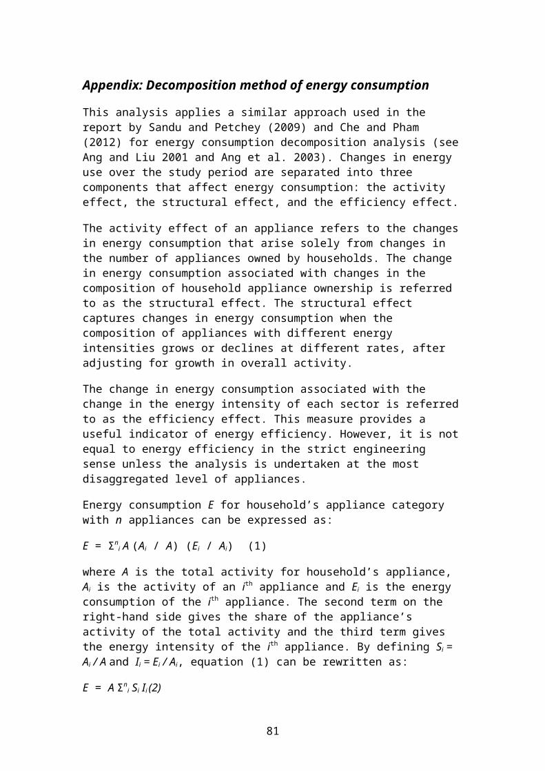
2009–10 2010–11 2011–12Jun Sep Dec Mar Jun Sep Dec Mar p

Thermal $m 3260 3856 3457 3007 3637 4253 4665 3985Copper e $m 1895 1978 2270 2041 2132 2212 2247 1854Diamonds cs $m 113 106 108 83 69 94 106 103Gems, other than diamonds $m 9 11 10 17 11 10 8 16Gold, refined $m 4209 2897 3600 3375 3143 3898 4210 3127IronIron ore and pellets $m 13156 58 14021 13707 16272 57 14208 12697Iron and steel s $m 396 315 399 292 297 344 305 135Lead e $m 539 410 616 501 532 522 625 501Manganese ore and concentrate

$m 447 228 441 384 353 322 315 232

Nickel es $m 1048 1057 920 1131 988 908 988 1046PetroleumCrude oil and other refinery feedstock

$m 3068 2937 2994 2638 3204 3111 3319 3258

LNG $m 2016 2861 2480 2463 2633 2951 3036 2871LPG $m 237 300 265 246 256 265 195 263Refinery products $m 158 137 104 78 208 225 92 –168Salt s $m 63 61 63 70 58 63 63 57Silver, refined $m 58 49 62 43 10 48 42 57Tin e $m 28 32 30 31 33 30 25 18TitaniumIlmenite concentrate $m 45 47 49 48 55 57 58 54Leucoxene concentrate $m 3 3 4 4 5 5 5 6Rutile concentrate $m 116 99 96 94 101 64 52 73Synthetic rutile s $m 74 73 77 79 85 78 73 76Titanium dioxide pigment $m 110 124 114 136 152 164 127 154Uranium oxide (U3O8) s $m 161 161 177 157 114 215 219 113Zinc e $m 701 600 551 570 651 567 633 533Zircon concentrate $m 81 101 122 166 143 117 87 60Other mineral resources f $m 1642 15549 1552 1425 1692 19880 4342 3756Total resources and energy g

$m 44721 45045 44599 40591 47445 51780 51125 43922

Total merchandise $m 61472 62620 61753 56794 65812 70632 69913 58695Total goods and services $m 74275 75680 74749 69145 78264 83186 82660 71204

a Includes aluminium hydroxide. b Metallic content of all ores, concentrates, intermediate products (where applicable) and refined metal. c Unsorted and sorted. d Includes metal content of ores and concentrates, intermediate products and nickel metal. e Value of all ores, concentrates, intermediate products (where applicable) and refined metal. f Derived as the difference between total resources and energy exports, below, and the sum of the above items. g Total resources and energy exports on an BREE balance of payments basis. p Preliminary. s BREE estimate.Sources: BREE; ABARES; Australian Bureau of Statistics, Canberra.

Table 20: Quarterly resources and energy export unit returns a2009–10 2010–11 2011–12 pJun Sep Dec Mar Jun Sep Dec Mar

Energy 318.8 335.5 308.7 331.3 369.5 389.6 383.8 353.2Metals and other minerals 288.9 301.8 284.8 311.8 319.6 321.4 296.4 261.1Total resources and energy 301.5 316.0 295.1 320.6 339.4 348.5 330.2 296.3

a Base: 1994-95 = 100. p Preliminary.Sources: BREE; ABARES; Australian Bureau of Statistics, Canberra.

81

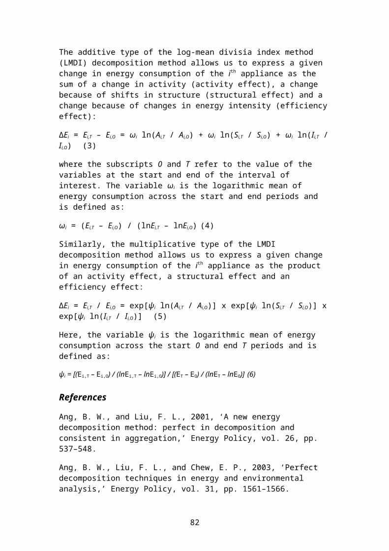
Table 21: Quarterly commodity imports2009–10 2010–11 2011–12Jun Sep Dec Mar Jun Sep Dec Mar

Quantity

Diamonds a '000 ct

300 334 565 156 133 259 151 107

Iron ore kt 1143 1476 1860 818 1288 1555 1314 841Ingot steel kt 475 597 433 401 437 445 433 492Ferroalloys kt 25 25 18 12 14 15 14 23PetroleumCrude oil and other refinery feedstock ML 7268 7684 7949 8060 8073 7184 7269 7878

Natural gas kt 773 1261 1218 1179 1140 1226 1089 1144Refinery products ML 4741 4317 4909 4317 5219 5646 6180 5085Phosphate rock kt 0 146 122 13 126 80 169 10ValueDiamonds a $m 105 106 108 94 90 101 107 101Gold b $m 2492 1292 1677 1182 1275 1822 2043 1507Iron ore $m 66 86 143 86 102 100 62 29Ingot steel $m 535 645 492 471 514 544 521 533Ferroalloys $m 33 40 35 24 28 28 27 26Nickel $m 13 15 11 49 47 54 39 48PetroleumCrude oil and other refinery feedstock $m 4115 4221 4423 5195 5739 4963 5173 5651

Natural gas $m 276 576 512 427 413 594 561 595Refinery products $m 2876 2463 2831 2915 3841 3936 4535 4048Phosphate rock $m 0 21 16 1 19 15 29 1Silver $m 7 23 103 111 254 572 187 93Other $m 383 382 314 483 383 420 586 378Total $m 10900 9870 10666 11039 12703 13150 13871 13011

a Includes sorted and unsorted, gem and industrial diamonds, and diamond dust and powder. b Refined and unrefined bullion. p Preliminary. Sources: BREE; ABARES; Australian Bureau of Statistics, Canberra.

Table 22: Quarterly private resources and energy exploration expenditure2009–10

2010–11 2010–11 2011–12

Dec Mar Jun Sep Dec MarEnergyPetroleumOnshore $m 748.6 756.5 206.4 153.2 186.4 248.6 278.3 163.1Offshore $m 2745.5 2558.9 643.2 612.9 662.9 531.6 618.7 432.9Coal $m 321.2 519.7 122.3 109.6 202.7 227.4 217.7 177.5Uranium $m 169.1 213.9 65.3 43.4 46.6 54.0 45.6 29.3Total energy $m 3984.4 4049.0 1037.2 919.1 1098.6 1061.6 1160.3 802.8Metals and other minerals Copper $m 201.7 323.1 81.8 70.9 101.5 108.9 114.6 98.7Diamonds $m na na na 0.6 na na 2.2 1.1Gold $m 575.4 652.2 167.3 146.4 178.2 184.2 200.0 168.8Iron ore $m 524.1 665.0 154.2 144.1 214.7 234.7 311.8 267.9Mineral sands $m na na na 6.2 na na 11.0 9.3Nickel, cobalt $m 203.9 270.9 62.4 67.6 71.6 73.6 49.3 64.1Silver, lead and $m 51.6 75.5 18.7 18.0 19.8 22.0 22.9 21.2

82

2009–10

2010–11 2010–11 2011–12

Dec Mar Jun Sep Dec MarzincOther $m 147.2 196.2 44.2 43.3 60.3 62.7 57.3 38.2Total metals and other minerals $m 1742.3 2217.7 536.8 497.1 658.1 702.0 769.1 669.3

Total expenditure $m 5726.7 6266.7 1574.0 1416.2 1756.7 1763.6 1929.4 1472.1

p Preliminary. na Not available.Sources: BREE; ABARES; Australian Bureau of Statistics, Canberra.

Table 23: Resources and energy pricesAlumina Aluminium Gold Iron ore Thermal

coalMetallurgical coal Crude oil

avg exportunit value

(high grade)LME cash

LondonAM fix




West Texas Intermediatespot price

Brent spot price

A$/t US$/t US$/oz A$/t A$/t A$/t US$/bbl US$/bbl2008–09 366.90 1867.66 873.99 105.83 131.16 293.94 70.29 68.752009–10 298.39 2016.26 1091.75 89.96 88.06 155.95 75.15 74.512010–11 321.54 2382.92 1371.59 143.50 97.37 212.12 89.29 96.002011January 322.97 2439.53 1360.48 138.56 97.45 185.88 89.51 96.32February 338.15 2508.13 1371.31 146.64 99.93 196.66 89.53 103.92March 347.39 2552.59 1422.85 137.11 101.09 206.07 102.91 114.44April 334.78 2662.67 1474.43 137.70 96.20 226.99 109.87 122.93May 340.88 2582.70 1512.19 135.40 99.06 258.92 101.28 114.37June 347.60 2555.41 1528.38 132.86 103.45 252.44 96.40 113.84July 334.64 2511.98 1568.53 127.35 104.80 251.91 97.14 116.42August 344.91 2391.91 1759.50 129.51 108.59 251.55 86.34 109.93September 330.60 2335.47 1775.85 125.95 108.24 247.03 85.61 109.79October 331.43 2172.19 1668.08 122.46 113.52 244.35 86.43 108.79November 320.50 2073.55 1735.98 121.33 114.10 235.78 97.13 110.49December 304.37 2018.60 1652.73 107.77 112.71 223.61 98.81 102.792012January 281.81 2137.23 1656.10 119.27 110.35 204.48 100.17 111.27February 283.09 2203.88 1743.10 114.83 106.23 187.19 102.31 119.10March 296.46 2184.80 1675.06 116.51 107.34 194.87 106.20 124.54

Uranium Copper Lead Zinc Silver Nickel Rutile Zircon

Industry spot price

(high grade) LME cash

LME cash

(high grade) LME cash

London fix LME cash avg export

unit value

avg export unit value

US$/lb US$/t US$/t US$/t USc/troy oz US$/t A$/t A$/t

2008–09 51.25 4918.86 1458.55 1403.25 1289.13 13322.04 609.23 788.702009–10 43.81 6691.13 2093.11 2065.82 1688.07 19390.25 664.64 494.192010–11 57.13 8670.65 2392.32 2242.53 2880.20 23962.89 793.37 551.922011January 73.00 9555.90 2601.65 2371.53 2841.25 25646.25 964.07 1344.31February 69.75 9867.55 2586.65 2465.10 3076.35 28252.00 928.66 1370.61March 62.50 9530.65 2624.20 2349.24 3581.35 26811.74 945.63 1409.93April 55.50 9483.19 2741.14 2372.36 4194.06 26328.89 945.98 1494.71May 57.50 8927.03 2426.31 2160.43 3675.00 24210.00 948.90 1586.10June 54.25 9045.43 2512.18 2230.48 3579.50 22354.09 969.58 1636.28

83

Alumina Aluminium Gold Iron ore Thermal coal

Metallurgical coal Crude oil


(high grade)LME cash

LondonAM fix




West Texas Intermediatespot price

Brent spot price

July 51.50 9619.24 2682.60 2390.55 3791.71 23731.19 1118.13 2011.05August 49.00 9038.84 2401.82 2211.27 4032.43 22068.41 1248.48 2215.28September 52.50 8702.77 2300.75 2078.25 3858.77 20416.82 1357.69 2324.96October 52.00 7338.81 1948.57 1859.14 3203.10 18886.43 1306.34 2408.35November 51.75 7551.77 1982.05 1916.11 3308.18 17882.05 1370.18 2542.15December 51.75 7565.57 2011.40 1911.76 3041.15 18170.24 1496.33 2518.462012January 52.00 8022.75 2089.77 1973.59 3076.86 19800.71 2695.24 2349.57February 52.00 8422.69 2126.12 2058.21 3414.05 20465.00 2459.20 2202.14March 51.00 8457.05 2061.45 2035.39 3295.32 18635.22 2468.59 2277.16

a Lump and fines. b US Department of Energy, Energy Information Administration. c Average of weekly restricted spot price published by The Ux Consulting Company. d London fix rate from May 2001; Handy and Harman, commercial bar, minimum 99.9 per cent prior to May 2001. e Bagged only after August 1999. g Bagged only after September 1999. s BREE estimate. na Not available.Sources: BREE; ABARES; Australian Bureau of Statistics, Canberra; London Metal Exchange; London Bullion Market Association; The Ux Consulting Company; US Department of Energy.

Table 24: Aluminium2009–10

2010–11 2010–11 2011–12

Dec Mar Jun Sep Dec Mar pProductionMineBauxiteQueensland kt 17707 19504 4813 4668 5061 5403 5600 4974Western Australia s kt 42899 42340 10864 10098 10578 10745 10833 11008Northern Territory kt 7204 6677 1721 1665 1550 1860 1916 1862Australia s kt 67810 68521 17398 16431 17189 18008 18349 17844 Alumina content s kt 25282 26039 6567 6257 6552 6935 7089 6774Smelter and refineryAlumina kt 20056 19041 4843 4471 4666 4726 4864 4866Aluminium (ingot metal) kt 1920 1938 488 476 486 490 493 481

ExportsQuantityBauxite kt 8023 8595 1772 2105 2663 2724 2803 2313Alumina ab kt 16653 16227 4141 3728 4094 4054 4103 4396Aluminium (ingot metal)Chinese Taipei kt 191 210 51 51 55 41 55 37Indonesia kt 102 104 20 34 29 31 33 36Japan kt 549 569 153 128 125 153 164 134Korea, Rep. of kt 333 352 100 87 78 77 64 61Malaysia kt 99 79 19 18 16 22 16 19Thailand kt 162 130 30 30 33 40 32 30Other kt 188 241 55 72 55 65 76 106Total kt 1624 1686 428 421 392 429 439 422Value

84

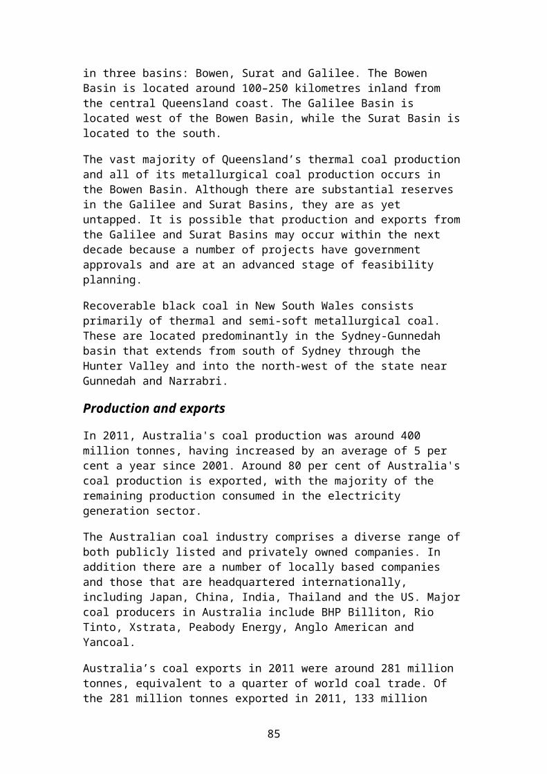
2009–10

2010–11 2010–11 2011–12

Dec Mar Jun Sep Dec Mar pBauxite $m 178 229 44 59 70 74 83 63Alumina a b $m 4969 5218 1275 1251 1397 1366 1306 1263Aluminium (ingot metal) $m 3838 4178 1046 1076 998 1043 982 923

ImportsQuantityBauxite kt 4 7 2 2 1 2 2 2Alumina a b kt 10 13 4 2 3 2 2 2Aluminium (ingot metal) kt 12 6 2 1 2 4 5 3

ValueBauxite $m 2 4 1 1 1 1 1 1Alumina a $m 12 14 4 3 3 3 2 4Aluminium (ingot metal) $m 27 18 4 4 5 10 12 7

PricesAlumina c A$/t 298 322 308 335 341 337 318 287AluminiumLME cash d US$/t 2016 2383 2343 2503 2597 2419 2088 2175Australia c A$/t 2363 2478 2443 2556 2547 2433 2235 2188

a Includes aluminium hydroxide. b Country details confidential. c Average export unit value. d High grade. p Preliminary. s BREE estimate.Sources: BREE; ABARES; Australian Bureau of Statistics, Canberra; London Metal Exchange.

Table 25: Coal2009–10

2010–11 2010–11 2011–12

Dec Mar Jun Sep Dec Mar pProductionMineBlack coal, rawUnderground 111.80 106.54 27.80 23.13 24.13 25.71 26.27 23.40Opencut 355.09 346.90 85.10 77.68 91.40 99.51 100.58 91.09New South Wales 190.62 204.85 52.62 50.67 51.37 56.36 53.74 52.53Queensland 263.40 239.12 57.91 47.77 61.79 66.49 70.75 59.59Western Australia a 8.39 5.00 1.25 1.25 1.25 1.25 1.25 1.25South Australia a 3.84 3.84 0.96 0.96 0.96 0.96 0.96 0.96Tasmania a 0.64 0.64 0.16 0.16 0.16 0.16 0.16 0.16Australia 466.89 453.44 112.90 100.81 115.53 125.22 126.85 114.49Black coal, saleableUnderground 87.87 76.11 20.19 16.47 17.51 19.14 18.98 s 16.78 sOpencut 274.66 268.69 68.38 60.30 67.58 73.89 74.41 s 67.94 sNew South Wales 147.30 156.95 40.52 38.93 38.88 43.46 40.78 40.07Queensland 204.07 179.39 45.94 35.73 44.10 47.45 50.50 s 42.54 sWestern Australia a 6.71 4.00 1.00 1.00 1.00 1.00 1.00 1.00South Australia a 3.84 3.84 0.96 0.96 0.96 0.96 0.96 0.96Tasmania a 0.62 0.62 0.15 0.15 0.15 0.15 0.15 0.15Australia 362.54 344.80 88.57 76.77 85.09 93.03 93.39 84.72 sBrown coal bVictoria 68.75 65.66 16.42 16.42 16.42 na na naExportsQuantity

85

2009–10

2010–11 2010–11 2011–12

Dec Mar Jun Sep Dec Mar pMetallurgical coal, high qualityBrazil 2.99 2.88 0.64 0.37 0.61 0.64 0.53 0.68China 15.52 9.64 4.28 1.42 1.00 1.76 2.95 3.43Chinese Taipei 3.49 4.06 1.24 0.85 0.98 1.05 1.07 1.11European Union 27 13.54 15.25 3.93 2.20 4.55 5.03 3.85 3.25India 24.51 25.19 6.17 4.84 7.29 6.05 5.79 5.12Japan 26.25 23.42 6.64 5.05 4.96 5.75 6.25 4.53Korea, Rep. of 6.89 8.10 2.56 1.85 1.80 2.41 2.90 2.48Other 4.53 3.06 1.13 0.56 0.59 1.30 1.12 1.21Total 97.72 91.60 26.60 17.15 21.79 23.99 24.46 21.81

Metallurgical coal, other cEuropean Union 27 2.07 1.82 0.57 0.27 0.35 0.25 0.67 0.30India 6.87 5.72 1.52 1.00 1.39 1.24 1.37 1.74Japan 22.21 19.19 5.00 4.89 4.54 4.09 5.25 3.74Other 28.40 22.12 6.30 4.16 4.98 5.75 5.42 7.08Total 59.55 48.85 13.38 10.32 11.25 11.34 12.71 12.85Total metallurgical coal 157.26 140.46 39.98 27.47 33.04 35.33 37.17 34.66Thermal coalChinese Taipei 19.55 20.12 5.35 3.97 4.95 5.30 4.84 3.90European Union 27 0.28 0.14 0.00 0.00 0.14 0.00 0.00 0.00China 13.92 16.67 2.45 2.29 4.37 5.43 1.45 5.42Japan 66.41 66.96 17.47 15.23 15.85 17.56 16.72 18.40Korea, Rep. of 24.84 28.19 6.69 7.11 6.61 7.54 8.21 6.67Other 23.90 27.90 8.06 3.95 8.89 9.25 11.37 7.90Total 134.98 143.32 37.57 30.26 36.45 39.66 41.14 36.86ExportsQuantity dOther coal 0.37 0.76 0.36 0.02 0.14 0.15 0.25 0.20ValueMetallurgical coalHigh quality 17060 21143 5520 3721 5810 6545 6237 4705Other quality 7465 8650 2129 1697 2337 2291 2470 2091Total metallurgical coal 24526 29793 7649 5417 8147 8836 8706 6796Thermal coal 11886 13956 3457 3007 3637 4253 4665 3985Other coal 35 106 47 4 28 26 37 27Total coal 36447 43854 11153 8428 11812 13115 13408 10808Coke 100 177 44 52 40 86 69 53Prices eMetallurgical coalHigh quality 174.59 230.81 207.52 216.93 266.63 272.80 254.93 215.74Other quality 125.37 177.06 159.09 164.35 207.69 202.03 194.36 162.69Thermal coal 88.06 97.37 92.01 99.35 99.78 107.21 113.39 108.10

a Quarterly data derived from annual BREE estimates. b Quarterly data not available. c Country details confidential for various time periods for Brazil, Chinese Taipei, Dem. Peoples Rep. of Korea, Italy, Pakistan and Republic of Korea–commencing from October 1996. d Quantity details for coke not available. e Average export unit value. p Preliminary. s BREE estimate. na Not available.Sources: BREE; ABARES; Australian Bureau of Statistics, Canberra; Coal Services Pty Limited; Queensland Government, Department of Mines and Energy.

86

Table 26: Copper2009–10

2010–11 2010–11 2011–12

Dec Mar Jun Sep Dec Mar pProductionMine sCopper ore and concentrate kt 3073 3507 917 856 846 902 901 833Copper content of all minerals producedNew South Wales a kt 155 158 37 42 43 46 46 39Queensland a kt 248 306 82 70 75 81 75 66Western Australia a kt 158 156 44 35 35 32 38 37South Australia kt 228 305 75 79 80 69 84 78Tasmania kt 29 26 6 6 6 6 8 8Australia a kt 819 952 244 232 239 235 252 228Smelter and refineryBlister copper (primary) b kt 381 459 119 108 116 105 112 115Refined copper (primary) s kt 395 485 123 117 125 114 121 124ExportsQuantityCopper concentrateChina c kt 612 566 147 130 180 172 147 163India kt 609 560 130 142 116 131 164 119Japan kt 371 303 65 80 77 122 91 56Korea, Rep. of kt 211 205 78 44 42 34 80 29Philippines kt 88 83 58 0 6 0 9 0Other kt 38 33 11 10 11 6 11 20

Total kt 1928 1750 490 407 431 466 503 386Refined copperChina c kt 119 121 35 31 19 35 51 37Chinese Taipei kt 45 54 15 9 19 15 13 11Germany kt 0 0 0 0 0 0 0 0Indonesia kt 12 24 5 5 6 8 7 6Japan kt 1 10 0 2 8 0 1 0Korea, Rep. of kt 15 26 4 14 4 0 1 0Malaysia kt 39 74 19 16 21 20 20 23Singapore kt 0 4 1 3 0 0 0 1Thailand kt 10 20 4 4 5 5 5 13Vietnam kt 25 28 9 4 6 4 3 6Other kt 6 14 3 3 4 2 3 1Total kt 271 375 96 90 92 89 105 97Copper content of all primary materials exported ds kt 805 877 235 208 222 219 255 212ValueCopper concentrate $m 4526 5130 1429 1176 1330 1480 1454 1116Refined copper $m 1980 3292 841 865 802 733 793 738Total $m 6506 8422 2270 2041 2132 2212 2247 1854Prices eLME cash US$/t 6691 8671 8637 9651 9152 9120 7485 8301Australia A$/t 7553 8752 8727 9620 8649 8658 7407 7869

a Includes copper cathode and copper precipitate. b Copper content. c Excludes Hong Kong. d Copper content of all ores and concentrates, slags, residues, intermediate products, refined copper, copper powder and flakes. e Based on LME cash, midday, high grade, 25 tonne

87

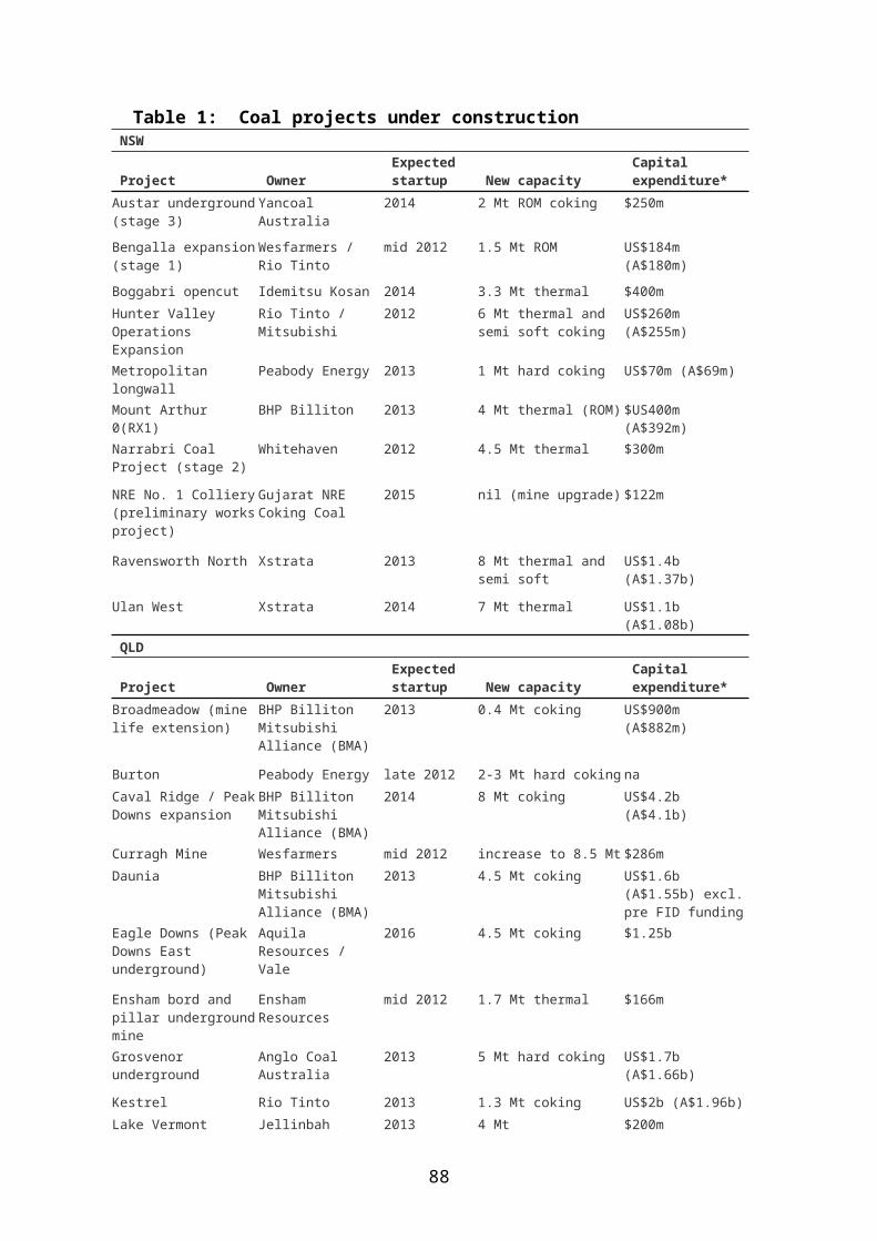
warrants. p Preliminary. s BREE estimate.Sources: BREE; ABARES; Australian Bureau of Statistics, Canberra; London Metal Exchange.

Table 27: Diamonds2009–10

2010–11 2010–11 2011–12

Dec Mar Jun Sep Dec Mar pProductionDiamondsNorthern Territory '000 ct 7 0 0 0 0 0 0 0Western Australia '000 ct 11131 8027 2283 1667 1607 2335 1953 2840Australia '000 ct 11138 8027 2283 1667 1607 2335 1953 2840ExportsQuantityDiamondsUnsorted s '000 ct 10299 9810 2678 2484 2020 2668 2938 2829Sorted Gem '000 ct 56 90 22 16 30 16 24 11 Industrial a '000 ct 0 0 0 0 0 0 0 0Total s '000 ct 10355 9900 2700 2500 2050 2684 2961 2840ValueDiamondsUnsorted s $m 294 225 61 53 41 61 67 75Sorted Gem $m 176 141 47 31 28 33 39 29 Industrial a $m 1 0 0 0 0 0 0 0Total s $m 471 366 108 83 69 94 106 103OpalsRough $m 6 6 2 2 1 2 1 0Cut and polished $m 28 35 7 12 9 7 6 13Total $m 33 41 9 14 9 9 6 14SapphiresRough $m 1 1 0 0 0 0 0 0Total $m 1 1 0 0 0 0 0 0Other gemstones b $m 5 8 2 3 2 1 1 2Total gemstones $m 40 49 10 17 11 10 8 16ImportsQuantityDiamondsUnsorted '000 ct 0 2 2 0 0 0 1 0Sorted Gem '000 ct 317 282 77 66 61 73 63 66 Industrial a '000 ct 2 1 0 0 0 47 8 4Dust and powder '000 ct 705 904 487 90 72 138 79 36ValueDiamondsUnsorted $m 0 0 0 0 0 0 0 0Sorted Gem $m 438 394 107 93 89 100 106 101 Industrial a $m 3 2 1 0 0 1 0 0Dust and powder $m 1 1 0 0 0 0 0 0Total $m 442 397 108 94 90 101 107 101

88

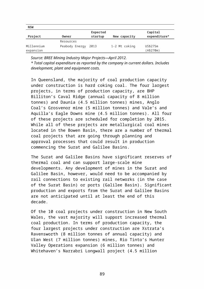
a Excludes dust, powder and unsorted diamonds. b Includes cut and polished sapphires from 1 July 2000. p Preliminary. s BREE estimate.Sources: BREE; ABARES; Australian Bureau of Statistics, Canberra.

Table 28: Gold2009–10

2010–11 2010–11 2011–12

Dec Mar Jun Sep Dec Mar pProductionMine sGold content of all minerals producedNew South Wales t 28 30 8 7 8 8 7 6Victoria t 7 6 1 1 1 2 1 1Queensland t 15 16 4 4 4 4 4 4Western Australia t 166 183 48 44 45 45 45 45South Australia t 10 16 4 4 4 3 3 3Tasmania t 4 4 1 1 1 1 1 1Northern Territory t 8 11 3 3 2 2 2 3Australia t 240 265 68 63 66 65 64 63RefineryPrimaryAustralian origin t 194 210 55 52 50 51 51 51Overseas origin t 69 71 19 18 17 15 17 14SecondaryAustralian origin t 3 4 1 1 1 1 1 1Overseas origin t 90 36 16 7 7 13 17 11Total t 356 321 90 78 75 81 86 77ExportsQuantityRefined and unrefined bullionHong Kong, China t 1 14 6 1 3 2 0 1India t 188 98 23 29 27 17 14 20Middle East t 0 0 0 0 0 0 0 0 United Arab Emirates t 0 0 0 0 0 0 0 0Singapore t 5 25 1 5 8 10 3 4Switzerland t 0 0 0 0 0 0 0 0Thailand t 35 56 8 22 12 16 8 5United Kingdom t 101 80 38 7 20 25 35 14Other t 4 9 2 5 1 7 5 1Total t 335 301 83 78 71 78 81 62ValueRefined $m 12996 13016 3600 3375 3143 3898 4210 3127ImportsValueRefined and unrefined bullion $m 7739 5426 1677 1182 1275 1822 2043 1507

PricesLondon AM fix US$/oz1092 1372 1369 1385 1505 1701 1686 1691Australia A$/oz 1236 1389 1391 1382 1425 1626 1666 1602

p Preliminary. s BREE estimate.Sources: BREE; ABARES; Australian Bureau of Statistics, Canberra; London Bullion Market Association.

89

Table 29: Iron2009–10

2010–11 2010–11 2011–12

Dec Mar Jun Sep Dec Mar pProductionIron ore and concentrate aWestern Australia kt 410206 436296 112212 101701 116793 123579 131613 122442South Australia kt 8275 9868 2622 2285 2611 2541 2754 2959 sTasmania s kt 2360 1840 442 319 521 506 632 512Northern Territory kt 2552 2011 443 327 661 600 450 450 sAustralia s kt 423393 450014 115720 104632 120586 127227 135450 126362 Iron content s kt 256567 273510 71746 64695 69738 70269 72297 69178Iron and steel bs kt 6886 7305 1887 1867 1704 1753 1214 1212ExportsQuantityIron ore and pelletsPellets, sinters and briquettes kt 2071 1634 584 118 421 463 393 879

Fines kt 281723 300734 79965 69302 78415 89332 91382 81419Lump and run of mine kt 106078 104508 28069 24318 26664 27519 29514 26175 China c kt 265565 279355 77138 62280 73301 81033 88635 78181 Chinese Taipei kt 10745 12613 3070 2775 3195 3353 2783 2830 European Union 27 kt 1576 986 341 153 327 161 313 158 Japan kt 75384 72893 18556 17904 17582 20730 18440 16327 Korea, Rep. of kt 36405 41029 9513 10625 11093 12038 11065 10926 Other kt 197 4 0 –0 0 0 53 50 Total iron ore and pellets kt 389872 406880 108618 93737 105499 117314 121289 108473

Iron content kt 242189 252473 67415 58159 65446 72690 75191 67268SteelIron and steel s kt 1549 1785 605 393 371 458 206 263Scrap kt 1606 1575 438 323 455 411 573 668

ValueIron ore and pelletsPellets, sinters and briquettes $m 210 260 83 18 78 84 75 135

Fines $m 23988 37297 9055 9212 9652 10264 9800 9129Lump and run of mine $m 10318 16647 4038 3917 4562 4648 4333 3433Total $m 35075 58387 14021 13707 16272 17992 16136 13073SteelIron and steel s $m 1120 1303 399 292 297 344 305 135Scrap $m 624 769 204 162 226 204 275 248 Total $m 1744 2072 603 454 523 548 580 383ImportsQuantityIron ore d kt 5094 5442 1860 818 1288 1555 1314 841Iron and steel kt 1736 1867 433 401 437 445 433 492Ferroalloys kt 71 69 18 12 14 15 14 23ValueIron ore d $m 259 417 143 86 102 100 62 29Iron and steel $m 1889 2121 492 471 514 544 521 533Ferroalloys $m 118 127 35 24 28 28 27 26Total $m 2265 2665 671 581 643 672 610 588PricesJapanese negotiated e USc/dmtu 179.65 230.18 163.97 183.62 248.28 248.60 211.18 212.66

90

a For use in iron and steel making; includes pellets for Tasmania. b Includes recovery from scrap. c Excludes Hong Kong. d Includes limonite ore used in the production of refined nickel products. e Indicative price: Australian hematite fines to Japan (fob), per dry metric tonne unit, for Japanese fiscal year commencing 1 April. p Preliminary. s BREE estimate.Sources: BREE; ABARES; Australian Bureau of Statistics, Canberra.

Table 30: Lead2009–10

2010–11 2010–11 2011–12

Dec Mar Jun Sep Dec Mar pProductionMine sLead ore and concentrates kt 880 934 264 195 234 218 233 272Lead content of all minerals producedNew South Wales kt 77 77 19 17 22 20 18 21Queensland kt 436 470 134 97 121 110 117 142Western Australia kt 32 78 35 9 2 4 2 2South Australia kt 10 7 2 2 2 2 2 3Tasmania kt 26 29 8 6 8 11 11 10Northern Territory kt 36 35 9 9 9 11 10 16Australia kt 617 697 207 140 164 157 160 195Smelter and refineryRefined lead (primary) a kt 189 190 57 49 51 42 45 54Domestic despatchesRefined lead kt 21 28 9 6 5 5 5 6ExportsQuantityLead concentrateChina kt 224 247 95 26 36 33 54 24European Union 27 kt 62 53 14 12 11 0 16 22Japan kt 65 67 16 17 17 17 22 11Korea, Rep. of kt 124 111 32 39 39 22 43 32Other kt 16 17 3 1 12 0 11 0Total kt 491 494 159 95 116 73 145 88Lead bullion bUnited Kingdom kt 151 93 37 20 12 39 29 46Total kt 151 93 37 20 12 39 29 46Refined leadChina kt 6 13 3 2 1 1 0 0Chinese Taipei kt 9 5 0 2 2 2 1 2India kt 40 35 7 9 11 8 8 8Indonesia kt 9 5 2 1 1 1 1 0Korea, Rep. of kt 48 32 8 9 9 9 12 8Malaysia kt 15 64 13 30 16 34 23 11South Africa kt 11 9 2 3 3 2 2 3Thailand kt 11 16 5 2 6 4 3 2Vietnam kt 21 20 6 3 5 3 3 4Other kt 16 15 4 3 5 7 5 3Total kt 186 213 50 64 58 70 58 43Lead content of all primary materials exported cs kt 658 676 192 158 177 168 189 156ValueLead concentrate $m 998 1301 396 288 359 215 389 255Lead bullion $m 409 248 101 51 30 138 109 161Refined lead $m 425 511 120 161 143 169 128 85

91

2009–10

2010–11 2010–11 2011–12

Dec Mar Jun Sep Dec Mar pTotal $m 1833 2059 616 501 532 522 625 501PricesLME cash d US$/t 2093 2392 2380 2605 2550 2458 1981 2109Australia e A$/t 2656 2635 2642 2776 2718 2617 2293 2231

a Includes lead content of lead alloys from primary sources. b Includes a substantial precious metal content, mainly silver. c Lead content of all ores, concentrates, slags, residues, bullion, and refined lead. d Based on LME cash, midday, standard grade, minimum 25 tonne warrants. e Pasminco Metals, 99.97–99.99 per cent, fob/for Port Pirie. p Preliminary. s BREE estimate. na Not available.Sources: BREE; ABARES; Australian Bureau of Statistics, Canberra; London Metal Exchange.

Table 31: Manganese2009–10

2010–11 2010–11 2011–12

Dec Mar Jun Sep Dec Mar pProductionManganese ore and concentrateWestern Australia s kt 1629 1786 415 435 551 570 544 525Northern Territory kt 4166 4997 1283 1013 1290 1339 1222 1346Australia s kt 5795 6784 1698 1448 1840 1909 1766 1871Manganese content s kt 2365 2756 687 594 754 783 726 764ExportsQuantityManganese ore and concentrate kt 5648 6190 1761 1681 1841 1787 1604 1419

ValueManganese ore and concentrate $m 1395 1407 441 384 353 322 315 232

PricesJapanese negotiated a US$/t 544.90 767.97 725.00 700.00 633.33 540.00 540.00 463.00

A$/t 616.68 777.81 736.19 697.65 598.59 514.67 533.72 438.66

a Indicative price: high grade ore (48 – 50 per cent Mn) to Japan for Japanese fiscal year commencing 1 April. p Preliminary. s BREE estimate.Sources: BREE; ABARES; Australian Bureau of Statistics, Canberra.

Table 32: Nickel2009–10

2010–11 2010–11 2011–12

Dec Mar Jun Sep Dec Mar pProduction asMineNickel contentWestern Australia kt 157 195 49 48 53 53 61 57Tasmania kt 0 0 0 0 0 0 0 0Australia kt 157 195 49 48 53 53 61 57Smelter and refineryIntermediate nickel kt 43 60 20 13 14 10 16 12Refined nickel, class 1 b kt 114 90 18 23 25 26 23 29Refined nickel, class 2 c kt 6 10 3 2 3 4 4 4Exports Quantity

92

2009–10

2010–11 2010–11 2011–12

Dec Mar Jun Sep Dec Mar pNickel d kt 221 210 50 51 54 56 57 63ValueOres and concentrates $m 704 859 107 282 254 145 328 243Intermediate products e $m 776 960 295 272 165 164 150 212Refined nickel, class 1 b $m 2285 2093 478 532 517 541 466 538Refined nickel, class 2 c $m 110 184 40 45 53 58 44 53Total $m 3875 4096 920 1131 988 908 988 1046ImportsValuePrimary nickel products f$m 182 279 64 68 84 95 76 68PricesLME cash g US$/t 19390 23963 23598 26899 24165 22047 18306 19603

A$/t 21916 24273 23949 26824 22872 20946 18094 18581

a Details of production of nickel metal, matte, oxide, sinter and nickel–cobalt sulphide are not available. b Products with a nickel content of 99 per cent or more. Includes electrolytic nickel, pellets, briquettes and powder. c Products with a nickel content of less than 99.8 per cent. Includes ferronickel, nickel oxides and oxide sinter. d Includes metal content of ores and concentrates, intermediate products and nickel metal. e Includes matte and speiss for further refining. f Includes matte, sinter and intermediate products; ferronickel, unwrought nickel metal and alloys and scrap. Also includes value of limonite ore used in the production of refined nickel products. g Average cash settlement price for melting grade refined nickel. p Preliminary. s BREE estimate.Sources: BREE; ABARES; Australian Bureau of Statistics, Canberra; London Metal Exchange.

Table 33: Petroleum2009–10

2010–11 2010–11 2011–12

Dec Mar Jun Sep Dec Mar pProductionFieldCrude oil d ML 16638 16115 4224 3330 3731 3691 3949 3339Condensate d ML 8945 8630 2178 1986 2049 2058 2005 1851Total d ML 25583 24745 6402 5316 5780 5749 5954 5190

Production rate d '000 bbl/day 442 428 443 367 400 397 412 359

LPG ML 4097 3907 948 913 924 1033 956 908Methane Mm3 44712 46851 11563 10809 11932 11562 10676 9867Ethane Mm3 311 295 64 65 80 103 96 75Coal seam gas Mm3 5100 5957 1490 1391 1501 1529 1526 1636RefineryRefinery input ML 37681 39871 10044 9926 10235 9862 9479 9894Refinery output LPG ML 1204 1467 349 372 371 304 292 330Automotive gasoline ML 16771 16643 4158 4011 4159 4098 3824 3773Aviation gasoline ML 104 91 22 20 25 24 26 25Aviation turbine fuel ML 5341 5448 1347 1363 1380 1414 1362 1426Kerosine ML 0 0 –0 0 0 0 na naHeating oil ML 35 16 3 3 2 3 6 2Automotive diesel oil ML 11720 12858 3153 3219 3225 3084 3242 3168Industrial and marine diesel fuel ML 3 0 0 0 0 0 0 0

Fuel oil (excl. refinery fuel) ML 846 952 264 251 235 223 228 243

93

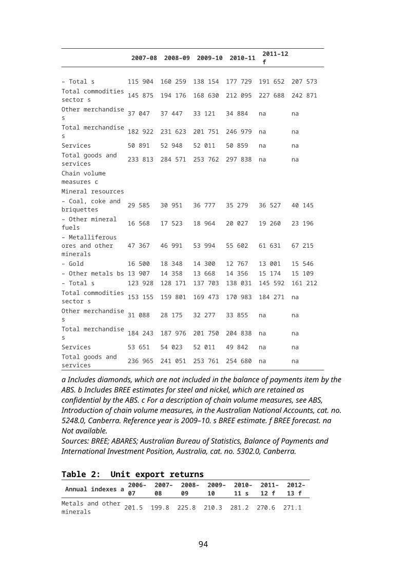
2009–10

2010–11 2010–11 2011–12

Dec Mar Jun Sep Dec Mar p

Lubricating oil basestock ML 74 64 27 11 2 –2 –2 0Bitumen ML 690 476 133 137 135 109 132 98Other products ML 412 377 71 96 112 63 84 77Total ML 37200 38393 9527 9483 9646 9318 9647 9520SalesLPGAutomotive use b ML 2083 2022 523 477 491 504 485 468Total ML 3795 3936 965 907 1011 989 890 866Automotive gasolinePremium unleaded ML 1843 2247 587 572 559 589 628 630Regular unleaded ML 12773 11388 2969 2791 2754 2810 2890 2837Other unleaded ML 4028 5090 1348 1268 1221 1262 1264 1244Total ML 18644 18725 4905 4632 4534 4662 4781 4711Aviation gasoline ML 80 79 19 18 20 21 21 20Aviation turbine fuel ML 6675 7068 1777 1756 1768 1845 1852 1824Kerosine ML 29 27 5 13 5 4 3 3Heating oil ML 7 5 2 1 1 0 0 2Automotive diesel oil ML 19044 20054 5061 4823 5335 5397 5511 5167Industrial and marine diesel fuel ML 26 7 3 1 0 0 0 0

Fuel oil ML 982 757 176 208 201 223 245 276Lubricating oil and greasesML 458 430 107 104 108 88 87 83Bitumen ML 814 719 183 196 194 148 204 194Other products ML 376 289 74 65 68 66 66 79Total ML 50929 52095 13276 12724 13244 13443 13663 13225ExportsQuantityCrude oil and other refinery feedstockChina ML 2185 3632 902 717 1046 1206 1158 948Chinese Taipei ML 261 266 15 18 129 15 16 266Japan ML 1931 2002 730 396 571 243 540 533Korea, Rep. of ML 3710 3794 1484 839 365 392 606 511New Zealand ML 235 56 1 2 1 1 1 3Singapore ML 3838 2649 477 784 644 713 1230 636United States ML 622 189 0 0 0 101 263 0Other ML 5283 7050 1847 1274 1848 1894 1041 1855Total ML 18064 19638 5456 4029 4604 4565 4856 4753LNG s Mt 17.87 19.96 5.18 4.85 4.98 4.59 4.77 4.56LPG ML 2776 2471 583 536 557 602 469 517Refinery productsAutomotive gasoline ML 222 175 38 0 78 117 0 21Aviation turbine fuel ML 72 12 10 0 0 1 1 4Diesel fuel c ML 187 117 7 33 71 42 6 70Fuel oil ML 109 194 41 20 65 60 40 90Aviation gasoline ML 32 20 7 4 3 6 11 9Lubricants ML 212 223 39 43 78 76 34 88Other products ML 16 19 12 2 –1 2 5 1Total ML 850 760 152 102 294 304 97 282Ships' and aircraft storesAviation turbine fuel ML 1985 1985 496 496 496 496 496 496Fuel oil ML 260 259 65 65 65 65 65 68Other products ML 41 38 8 9 15 18 7 566

94

2009–10

2010–11 2010–11 2011–12

Dec Mar Jun Sep Dec Mar p

Total ML 2285 2282 569 570 576 579 568 1130ImportsQuantityCrude oil and other refinery feedstockIndonesia ML 4178 4805 1596 1000 1019 662 959 782Malaysia ML 5319 5929 1431 1337 1274 866 1335 1604Middle East Saudi Arabia ML 478 156 92 0 64 0 0 216 United Arab Emirates ML 3846 4683 926 1037 1688 1260 1566 887 Other ML 43 0 0 0 0 0 0 0 Total Middle East ML 4367 4880 1018 1037 1793 1260 1566 1103New Zealand ML 2569 2565 621 658 640 578 498 587Papua New Guinea ML 1580 1612 220 566 409 305 399 408Singapore ML 605 497 164 139 162 104 96 128Vietnam ML 3904 2554 777 428 558 831 356 262Other ML 4762 8923 2121 2894 2218 2577 2058 3004Total ML 27284 31766 7949 8060 8073 7184 7269 7878Natural gas kt 4149 4799 1218 1179 1140 1226 1089 1144Refined products LPG ML 1067 888 327 136 191 411 168 156Automotive gasoline ML 3884 2653 712 827 599 775 1176 897Aviation turbine fuel ML 2168 2086 633 462 485 642 646 466Diesel fuel c ML 8668 8820 2040 1815 2888 2704 2920 2703Fuel oil ML 1797 1559 505 420 375 361 451 457Lubricants ML 415 463 113 124 123 132 141 128Other products ML 1966 2293 579 533 558 619 677 278Total ML 19967 18762 4909 4317 5219 5646 6180 5085ValueCrude oil and other refinery feedstock $m 15031 19578 4423 5195 5739 4963 5173 5651

Natural gas $m 1219 1929 512 427 413 594 561 595Refined productsLPG $m 405 376 146 58 87 167 65 78Automotive gasoline $m 2447 1838 445 597 471 599 905 721Aviation turbine fuel $m 1283 1440 399 351 378 482 503 364Diesel fuel c $m 5270 6237 1288 1356 2309 2053 2307 2160Fuel oil $m 910 836 241 238 229 217 297 312Lubricants $m 519 671 159 174 189 212 228 191Other products $m 1683 2581 665 568 591 801 791 819Total $m 11296 12050 2831 2915 3841 3936 4535 4048Total $m 27546 33557 7766 8537 9993 9494 10269 10295PricesDubai US$/bbl 74.19 92.18 84.25 100.26 110.82 107.19 100.21 106.00West Texas intermediate US$/bbl 75.15 89.29 84.79 94.41 102.27 89.59 94.10 102.90Brent US$/bbl 74.51 96.00 86.42 105.21 116.81 111.98 107.40 118.29Tapis US$/bbl 77.42 100.59 90.73 109.34 123.85 118.91 115.43 na

a Commercial sales plus field and plant usage. b This is a minimum level and includes only direct sales by the oil industry. The data do not include volumes sold to distributors etc. that are subsequently used or sold for automotive use. c Includes automotive diesel oil and industrial and marine diesel fuel. d Energy Quest. p Preliminary. s BREE estimate.

95

Sources: BREE; ABARES; Australian Bureau of Statistics, Canberra; Department of Resources, Energy and Tourism, Canberra; Energy Quest; US Department of Energy, Energy Information Administration.

Table 34: Petroleum production, by basinTable 34 habitually contains production statistics for crude oil, condensate, LPG, ethane and natural gas by basin on a quarterly and annual basis. Data for this table are sourced from the Australian Petroleum Statistics, which are collected via voluntary industry reporting by the Department of Resources, energy and Tourism.

The Department of Resources, energy and Tourism and ABARES conducted a review of the Australian Petroleum Statistics that identified issues affecting the coverage and quality of petroleum data. The Department of Resources, energy and Tourism is currently liaising with industry to resolve data-reporting issues and improve the coverage of the Australian Petroleum Statistics. Table 34 will be updated once these issues are resolved.

Table 35: Sales of petroleum products, by state marketing areaNSW Vic. QLD WA SA Tas. NT Aust.

ML ML ML ML ML ML ML ML2010–11LPG bAutomotive use c 563 874 191 149 225 13 7 2022Total 1206 1396 583 284 374 65 28 3936Automotive gasolinePremium unleaded 1003 398 433 249 91 51 21 2247Regular unleaded 2160 3612 2515 1576 1090 331 104 11388Other unleaded d 2996 629 1181 149 116 19 0 5090Total 6159 4640 4130 1973 1296 401 126 18725 of which sales to retailers 5172 3864 3166 1725 973 198 67 15165Aviation gasoline 14 14 21 15 6 1 7 79Aviation turbine fuel 3191 1138 1477 836 239 27 159 7068Kerosine 1 3 19 0 0 1 1 27Heating oil 0 1 0 0 0 4 0 5Automotive diesel oil 4352 3269 5501 4535 1427 367 603 20054 of which sales to retailers 1682 1410 1388 879 317 34 57 5766Industrial and marine diesel fuel 6 0 0 0 0 0 0 7

Fuel oil e 192 269 128 168 0 0 0 757Lubricating oil and greases 130 102 97 62 28 5 5 430Bitumen 190 123 264 65 59 13 4 719Other products f 214 31 20 12 10 0 1 289Total 15655 10988 12241 7952 3440 885 934 52095

a Includes Australian Capital Territory. b Includes sales for petrochemical feedstock. c This is a minimum level and includes only direct sales by the oil industry. The data do not include volumes sold to distributors etc. that are subsequently used or sold for automotive use. d Includes proprietary brand and other blends. e Excludes refinery fuel. f Sales of LPG for petrochemical feedstock are included in LPG sales. p Preliminary.Source: Department of Resources, Energy and Tourism, Canberra.

96

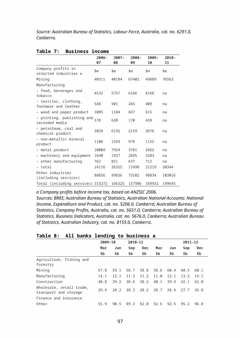
Table 36: Phosphate2009–10

2010–11 2010–11 2011–12

Dec Mar Jun Sep Dec Mar pImportsQuantityPhosphate rockChina kt 1 0 0 0 0 0 1 0Morocco kt 73 288 81 0 80 55 98 0Nauru kt 0 74 30 0 34 0 42 0Togo kt 0 0 0 0 0 0 0 0Other kt 11 46 11 13 12 25 28 10Total kt 85 408 122 13 126 80 169 10PhosphatesDiammonium a kt 203 185 27 112 33 3 13 68Monammonium b kt 433 753 154 388 152 5 128 365High analysis c kt 160 297 171 82 24 5 26 41ValuePhosphate rock $m 10 57 16 1 19 15 29 1PhosphatesDiammonium a $m 107 109 15 67 19 2 9 35Monammonium b $m 203 437 85 225 93 4 84 203High analysis c $m 36 81 42 27 8 2 12 14PricesAustralia d A$/t 253.11 133.13 129.36 110.82 147.09 187.40 172.05 121.38

a P2O5 equivalent: 46 per cent. b P2O5 equivalent: 50 per cent. c P2O5 equivalent: 48 per cent. d Average import unit value. p Preliminary. na Not available.Sources: Australian Bureau of Statistics, Canberra; Queensland Government, Department of Mines and Energy; Government of South Australia, Primary Industries and Resources South Australia.

Table 37: Salt2009–10

2010–11 2010–11 2011–12

Dec Mar Jun Sep Dec Mar pProduction sAustralia a kt 11772 11562 3091 2885 2494 3067 2957 2544Exports sQuantityBulk, bagged and table kt 11185 11162 2772 3081 2595 2793 2802 2523ValueBulk, bagged and table $m 247 251 63 70 58 63 63 57Prices sAustralia b A$/t 22.09 22.50 22.55 22.69 22.29 22.49 22.50 22.49

a Excludes Victoria. b Average export unit value. p Preliminary. s BREE estimate.Sources: BREE; ABARES.

Table 38: Silver2009–10

2010–11 2010–11 2011–12

Dec Mar Jun Sep Dec Mar pProductionMine s

97

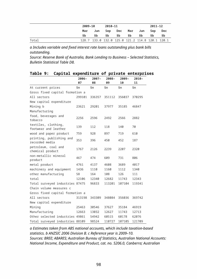
2009–10

2010–11 2010–11 2011–12

Dec Mar Jun Sep Dec Mar pSilver content of all minerals producedNew South Wales t 82 73 18 19 20 17 18 23Queensland t 1527 1483 417 272 376 321 384 338Western Australia t 60 51 12 12 14 22 15 13South Australia t 15 34 9 8 8 7 7 6Tasmania t 78 110 23 21 46 48 43 34Northern Territory t 47 42 12 7 12 14 13 13Australia t 1809 1792 491 340 476 428 481 426RefineryRefined silver t 701 712 174 189 212 250 247 168ExportsQuantityRefined silver bullion t 420 198 79 41 7 41 44 56

ValueRefined silver a $m 254 164 62 43 10 48 42 57ImportsValueRefined silver bullion $m 107 490 103 111 254 572 187 93

PricesWorld b USc/oz 1688 2880 2643 3186 3796 3898 3188 3263Australia c A$/kg 609 920 841 991 1178 1128 948 992

a Includes refined bullion, powder, unwrought silver and semi-manufactured forms. b London Bullion Market Association, fixed rate. c Pasminco Metals, fob/fot Port Pirie. p Preliminary. s BREE estimate.Sources: BREE; ABARES; Australian Bureau of Statistics, Canberra; London Bullion Market Association.

Table 39: Tin2009–10

2010–11 2010-11 2011–12

Dec Mar Jun Sep Dec Mar pProductionMineTin content of all minerals producedWestern Australia s t 13562 12000 3000 3000 3000 1500 1500 70Tasmania t 6267 6410 1600 1600 1600 1600 1600 1426Australia s t 19829 18410 4600 4600 4600 3100 3100 1496ExportsQuantityTin concentrate t 11922 12835 4812 2594 2438 2538 3478 1859Refined tin t 29 5 1 0 3 10 6 0Tin content of primary materials exported as t 6031 5431 1359 1279 1220 1244 1246 922

ValueTin concentrate $m 101 126 30 31 33 29 25 18Refined tin $m 0 0 0 0 0 0 0 0Total $m 101 126 30 31 33 30 25 18ImportsQuantity

98

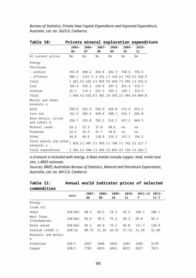
2009–10

2010–11 2010-11 2011–12

Dec Mar Jun Sep Dec Mar pRefined tin t 752 673 167 216 146 187 127 190ValueRefined tin $m 14 18 4 6 4 5 3 4PricesLME b US$/t 16202 23960 26001 24200 25400 23200 22100 17339

a Tin content of tin ores and concentrates and refined tin. b LME official close. p Preliminary. s BREE estimate.Sources: BREE; ABARES; Australian Bureau of Statistics, Canberra; London Metal Exchange.

Table 40: Titanium minerals2009–10

2010–11 2010–11 2011–12

Dec Mar Jun Sep Dec Mar pProduction sIlmenite concentrateNew South Wales kt 90 90 23 23 23 23 23 23Queensland kt 186 186 47 47 47 47 47 47Victoria kt 27 87 26 26 26 26 22 25South Australia kt 38 173 42 39 46 46 43 44Western Australia kt 1058 739 189 166 180 185 195 182Northern Territory kt 0 0 0 0 0 0 0 0Australia kt 1398 1275 326 300 322 326 329 319Leucoxene concentrateNew South Wales kt 67 134 32 36 41 41 41 41Victoria kt 8 10 3 3 3 3 3 3South Australia kt 0 0 0 0 0 0 0 0Western Australia kt 48 56 14 14 15 14 14 14Northern Territory kt 0 0 0 0 0 0 0 0Australia kt 123 200 48 53 58 57 57 57Rutile concentrateNew South Wales kt 69 80 20 20 20 20 20 20Victoria kt 108 235 58 57 59 60 50 34Queensland kt 86 75 19 19 19 19 19 18South Australia kt 6 27 3 6 15 19 16 17Western Australia kt 93 50 13 10 10 10 10 10Australia kt 361 467 112 111 122 127 114 98Synthetic rutile kt 553 542 141 133 129 118 123 105Titanium dioxide pigment kt 222 204 51 51 51 51 51 51

ExportsQuantityIlmenite concentrate akt 1763 1804 448 433 496 518 527 492Leucoxene concentrate kt 18 27 7 7 8 8 8 8

Rutile concentrate s kt 575 491 130 123 98 85 82 81Synthetic rutile s kt 513 517 132 131 123 136 136 141Titanium dioxide pigment kt 181 195 44 50 53 51 41 51

ValueIlmenite concentrate a$m 197 198 49 48 55 57 58 54Leucoxene concentrate $m 11 17 4 4 5 5 5 6

99

2009–10

2010–11 2010–11 2011–12

Dec Mar Jun Sep Dec Mar pRutile concentrate s $m 382 390 96 94 101 64 52 73Synthetic rutile s $m 269 315 77 79 85 78 73 76Titanium dioxide pigment $m 448 527 114 136 152 164 127 154

Prices bIlmenite concentrateBulk s A$/t112 110 110 110 110 110 110 110Rutile concentrateBagged A$/t1 949 621 624 624 685 638 643Titanium dioxide pigment A$/t2477 2708 2579 2703 2850 3217 3134 3033

a From January 1992, bulk only. b Average export unit value. p Preliminary. s BREE estimate. na Not available.Sources: BREE; ABARES; Australian Bureau of Statistics, Canberra.

Table 41: Uranium2009–10

2010–11 2010–11 2011–12

Dec Mar Jun Sep Dec MarProductionMine Uranium oxide (U3O8) t 7109 7069 2209 1668 1185 2070 2019 1618Uranium (U content)South Australia t 2414 3724 885 975 934 899 839 853Northern Territory t 3614 2270 988 439 70 856 873 519Australia t 6028 5995 1873 1414 1005 1755 1712 1372Exports asQuantityUranium oxide (U3O8) s t 7555 6950 2104 1701 1227 2070 2019 1618

ValueUranium oxide (U3O8) s $m 757 610 177 157 114 215 219 154

PricesUranium oxide (U3O8)Industry spot b US$/lb 43.81 57.13 58.50 68.42 55.75 51.00 51.83 51.67Australia cs A$/kg 100.23 87.71 84.17 92.57 92.57 103.70 108.47 95.11

a ABS confidentiality: no country details to July 2009 and no details from August 2009. b Average of weekly restricted spot price, published by The Ux Consulting Company. c Average export unit value. p Preliminary. s BREE estimate.Sources: BREE; ABARES; Australian Bureau of Statistics, Canberra; Department of Resources, Energy and Tourism; The Ux Consulting Company.

Table 42: Zircon2009–10

2010–11 2010–11 2011–12

Dec Mar Jun Sep Dec Mar pProduction sZircon concentrateNew South Wales kt 53 70 14 21 21 21 21 22Victoria kt 92 197 47 48 53 58 59 35

100

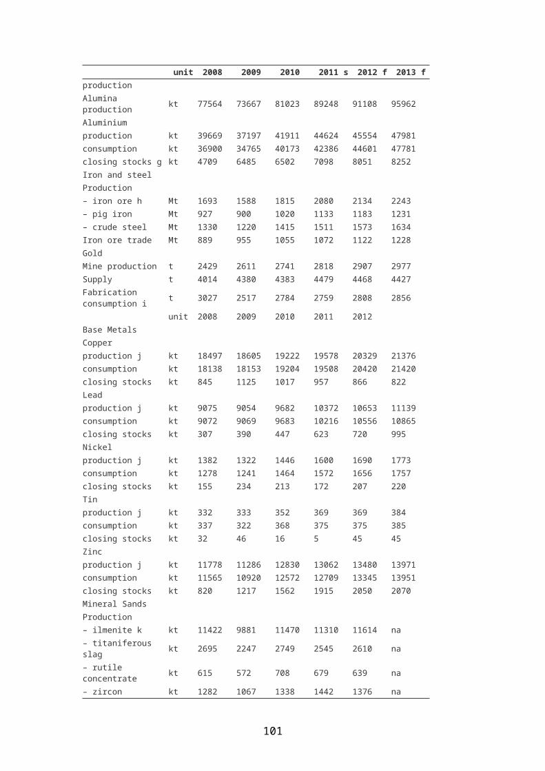
2009–10

2010–11 2010–11 2011–12

Dec Mar Jun Sep Dec Mar pQueensland kt 49 40 10 10 10 15 15 15South Australia kt 46 249 54 71 71 93 69 67Western Australia kt 168 118 30 27 28 24 27 24Northern Territory kt 0 0 0 0 0 0 0 0Australia kt 408 674 156 177 183 211 191 164Exports sQuantityZircon concentrate kt 748 963 228 260 247 237 219 196ValueZircon concentrate $m 370 532 122 166 143 117 87 60Prices aZircon concentrateAll grades – bagged A$/t 1049 1322 1097 1380 1585 2162 2488 2275

a Average export unit value. p Preliminary. s BREE estimate.Sources: BREE; ABARES; Australian Bureau of Statistics, Canberra.

Table 43: Zinc2009–10

2010–11 2010–11 2011–12

Dec Mar Jun Sep Dec Mar pProductionMine sZinc ore and concentrates kt 2600 2947 771 647 820 879 847 830Zinc content of all minerals producedNew South Wales kt 102 102 26 23 28 29 32 28Queensland kt 858 1009 271 223 268 255 262 255Western Australia kt 109 79 20 24 13 34 19 25South Australia kt 23 17 5 4 4 5 5 6Tasmania kt 84 92 24 21 23 26 27 28Northern Territory kt 186 181 46 42 48 52 49 47Australia kt 1362 1479 391 337 384 401 394 389Smelter and refineryRefined zinc (primary) kt 515 499 126 123 125 126 133 131 sDomestic despatchesRefined zinc kt 71 65 7 17 19 15 17 naExportsQuantityZinc concentrates Belgium–Luxembourg kt 26 51 13 13 13 13 13 13China kt 1146 973 374 164 187 269 373 153Germany kt 11 84 0 44 31 19 11 40India kt 39 44 5 9 10 9 10 12Japan kt 285 249 108 26 70 77 86 59Korea, Rep. of kt 333 316 52 116 119 101 100 119Netherlands kt 217 293 72 70 71 50 54 98Spain kt 116 234 0 63 92 57 0 61Thailand kt 100 64 11 9 25 0 21 10Other kt 0 9 5 0 0 0 0 0Total kt 2271 2317 639 514 617 594 668 565Refined zinc China kt 109 73 8 17 28 25 44 26

101

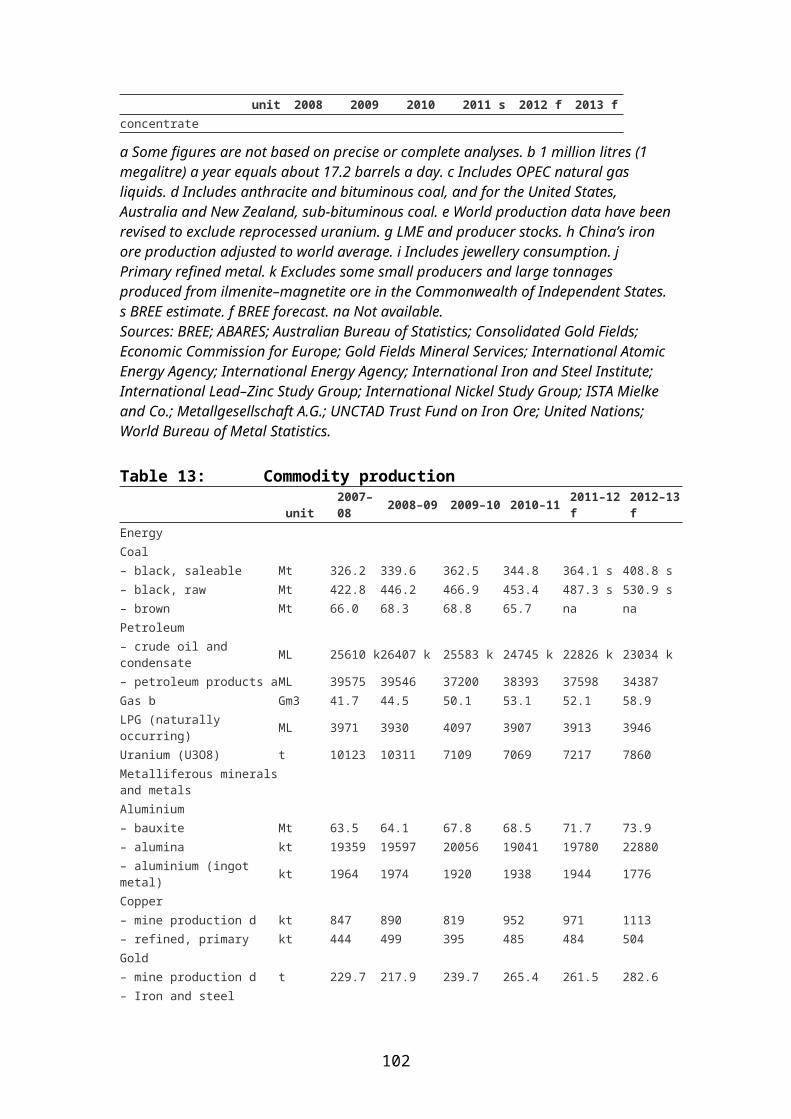
2009–10

2010–11 2010–11 2011–12

Dec Mar Jun Sep Dec Mar pChinese Taipei kt 91 84 23 15 23 17 22 17Hong Kong, China kt 61 61 13 15 16 18 16 6India kt 6 6 1 2 2 1 1 1Indonesia kt 20 22 6 5 4 4 4 3Korea, Rep. of kt 6 8 3 1 0 0 0 0Malaysia kt 26 29 7 7 8 7 6 7New Zealand kt 7 11 3 2 3 2 3 2Saudi Arabia kt 7 6 2 2 2 0 1 1United States kt 21 73 0 31 20 20 20 48Other kt 71 38 7 7 17 5 6 5Total kt 425 410 73 103 121 100 122 117Zinc content of all primary materials exported as kt 1482 1494 357 343 411 372 433 386ValueZinc concentrates $m 1237 1479 388 334 389 350 388 311Refined zinc $m 977 893 164 235 263 217 245 222Total $m 2214 2373 551 570 651 567 633 533PricesLME cash b US$/t 2066 2243 2315 2393 2250 2224 1912 2022Australia c A$/t 2265 2458 2545 2575 2387 2327 2112 2094

a Zinc content of all ores, concentrates, slags, residues, intermediate products, refined zinc, zinc powders, flakes and dust. b LME cash, midday, registered brands, minimum 98 per cent, 25 tonne warrants. c EZ Industries, Prime Western, 98.5 per cent. p Preliminary. s BREE estimate. na Not available.Sources: BREE; ABARES; Australian Bureau of Statistics, Canberra; London Metal Exchange.

102

BREE contacts

Executive Director/Chief

Economist – BREE

Quentin Grafton [email protected]

(02) 6243 7483

Deputy Chief Economist/Research

Director

Roger Rose [email protected]

(02) 6243 7583

Modelling & Policy Integration –

Program Leader

Arif Syed [email protected]

(02) 6243 7504

Resources Program – Program

Leader

Alan Copeland [email protected]

(02) 6243 7501

Energy and Quantitative Analysis –

Program Leader

Nhu Che [email protected]

(02) 6243 7539

Data & Statistics Program –

Program Leader

Geoff Armitage [email protected]

(02) 6243 7510

103







Documents

Resources and Energy Quarterly - March Quarter 2012 · Web viewIn the review section of Resources and Energy Quarterly there is a review of the on-going euro crisis; a review of an