Resource Use and Selection

• Habitat (resource) Selection

• Levels of Selection

• Multiple Scale Studies

• Methodological Issues

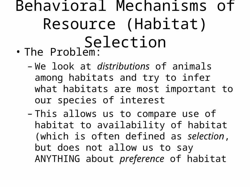
Behavioral Mechanisms of Resource (Habitat) Selection

• The Problem:– We look at distributions of animals among

habitats and try to infer what habitats are most important to our species of interest

– This allows us to compare use of habitat to availability of habitat (which is often defined as selection, but does not allow us to say ANYTHING about preference of habitat

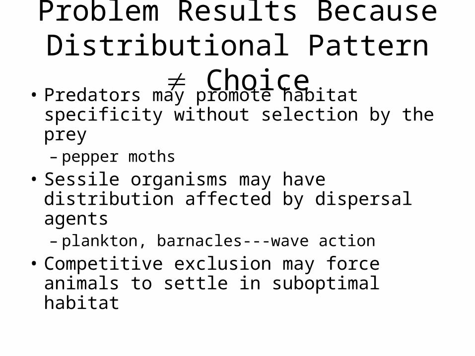
Problem Results Because Distributional Pattern Choice

• Predators may promote habitat specificity without selection by the prey– pepper moths

• Sessile organisms may have distribution affected by dispersal agents– plankton, barnacles---wave action

• Competitive exclusion may force animals to settle in suboptimal habitat

The Solution?

• Detailed behavioral study– Understand the mechanism that produces

distributional pattern– If all else is equal is a certain habitat selected

over another?– Usually takes lab and field approach

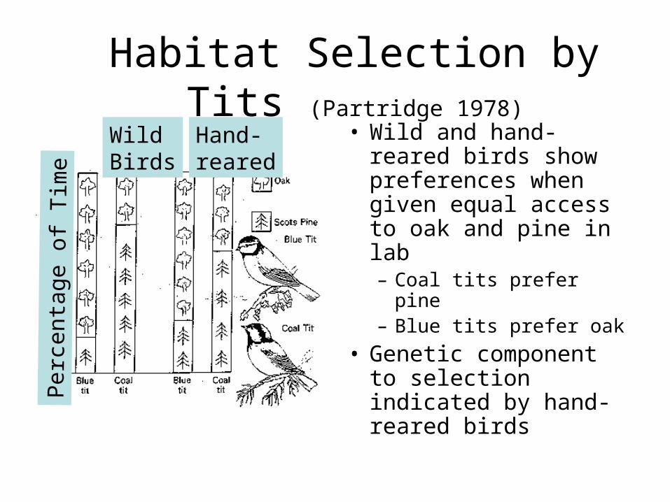
Habitat Selection by Tits (Partridge 1978)

• Wild and hand-reared birds show preferences when given equal access to oak and pine in lab– Coal tits prefer pine– Blue tits prefer oak

• Genetic component to selection indicated by hand-reared birds

Per

cent

age

of T

ime

WildBirds

Hand-reared

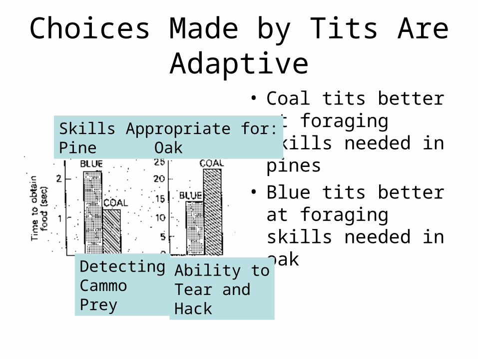
Choices Made by Tits Are Adaptive

• Coal tits better at foraging skills needed in pines

• Blue tits better at foraging skills needed in oak

DetectingCammoPrey

Ability toTear andHack

Skills Appropriate for:Pine Oak

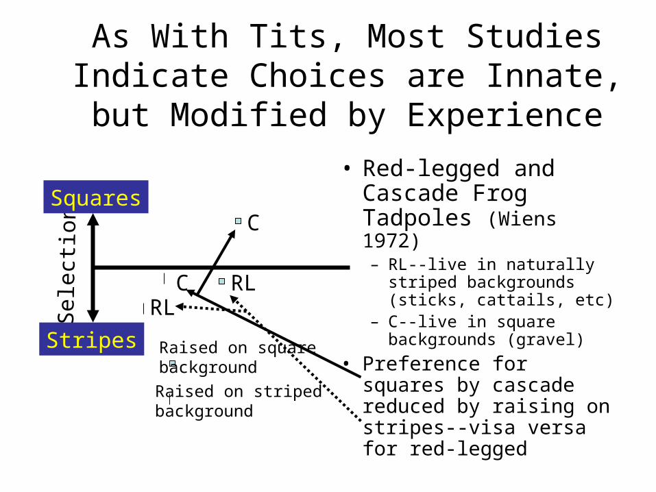
As With Tits, Most Studies Indicate Choices are Innate, but Modified by

Experience

• Red-legged and Cascade Frog Tadpoles (Wiens 1972)– RL--live in naturally striped

backgrounds (sticks, cattails, etc)

– C--live in square backgrounds (gravel)

• Preference for squares by cascade reduced by raising on stripes--visa versa for red-legged

Sel

ecti

on

Stripes

SquaresC

RL

Raised on stripedbackground

Raised on squarebackground

CRL

Features Important in Habitat Selection (Verner 1975, Hilden 1965, Klopfer and Hailman 1965)

• Food• Nest Sites• Song Posts, Hunting Perches, Shelter• Terrain• Vegetation• Previous Experience• Other Animals

– Social stimulation• Colonial Animals--young often settle in established

colonies (Herring Gulls, Drost 1958)

How Are Multiple Cues Integrated?

• Summation (Hilden 1965)– each cue is added or subtracted to form a total score

for a habitat– if score exceeds some threshold, animal settles

• Niche Gestalt (James 1971)– habitat is responded to as a whole

• Hierarchical Selection (Wiens and Rotenberry 1981)– large scale vs. fine scale selection

Natural Ordering of Selection Process (Johnson 1980)

• First order– Selection of the physical or geographical range of a a

species• Second order

– Placement of the home range of an individual or social group within the species’ range

• Third order– Use of various habitat components within the home

range• Fourth order

– Selection of resources from within areas within the home range (food selection at a foraging site, for example)

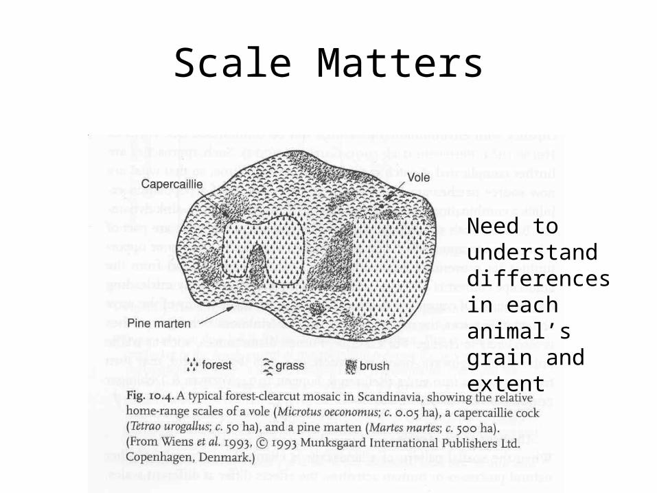
Scale Matters

Need to understand differences in each animal’s grain and extent

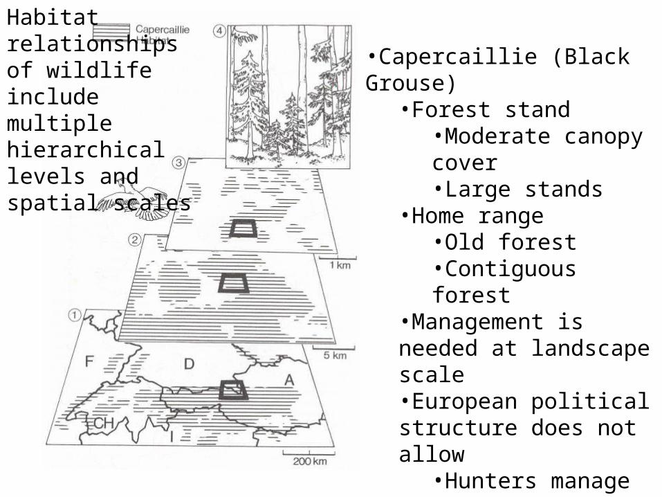
•Capercaillie (Black Grouse)•Forest stand

•Moderate canopy cover•Large stands

•Home range•Old forest•Contiguous forest

•Management is needed at landscape scale•European political structure does not allow

•Hunters manage at stand scale for habitat structure

(Storch 1997)

Habitat relationships of wildlife include multiple hierarchical levels and spatial scales

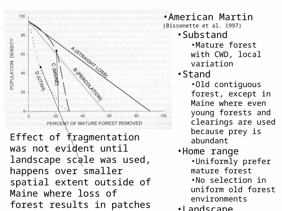
•American Martin (Bissonette et al. 1997)

•Substand•Mature forest with CWD, local variation

•Stand•Old contiguous forest, except in Maine where even young forests and clearings are used because prey is abundant

•Home range•Uniformly prefer mature forest•No selection in uniform old forest environments

•Landscape•Consistent selection for areas with ~75% forest

Effect of fragmentation was not evident until landscape scale was used, happens over smaller spatial extent outside of Maine where loss of forest results in patches of unsuitable habitat interspersed with suitable habitat

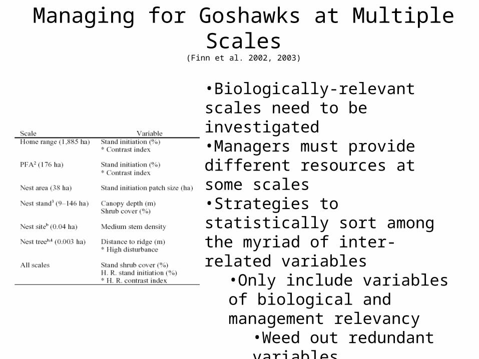
Managing for Goshawks at Multiple Scales(Finn et al. 2002, 2003)

•Biologically-relevant scales need to be investigated•Managers must provide different resources at some scales•Strategies to statistically sort among the myriad of inter-related variables

•Only include variables of biological and management relevancy

•Weed out redundant variables•Conduct single scale analysis and later combine best predictors at each scale to determine important scales

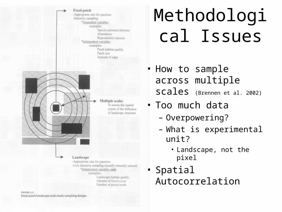
Methodological Issues

• How to sample across multiple scales (Brennen et al. 2002)

• Too much data– Overpowering?– What is experimental

unit?• Landscape, not the pixel

• Spatial Autocorrelation

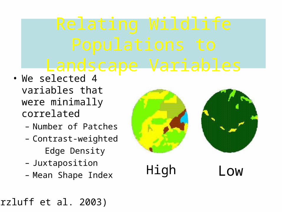
Relating Wildlife Populations to Landscape Variables

• We selected 4 variables that were minimally correlated – Number of Patches– Contrast-weighted

Edge Density– Juxtaposition– Mean Shape Index High Low

(Marzluff et al. 2003)

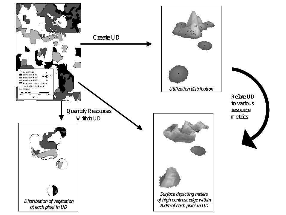
Create UD

Quantify ResourcesWithin UD

Relate UD to various resource metrics

Utilization distribution

Surface depicting metersof high contrast edge within200m of each pixel in UD

Distribution of vegetationat each pixel in UD

Create UD

Quantify ResourcesWithin UD

Relate UD to various resource metrics

Utilization distribution

Surface depicting metersof high contrast edge within200m of each pixel in UD

Distribution of vegetationat each pixel in UD

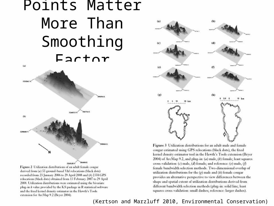
Points Matter More Than Smoothing

Factor

(Kertson and Marzluff 2010, Environmental Conservation)

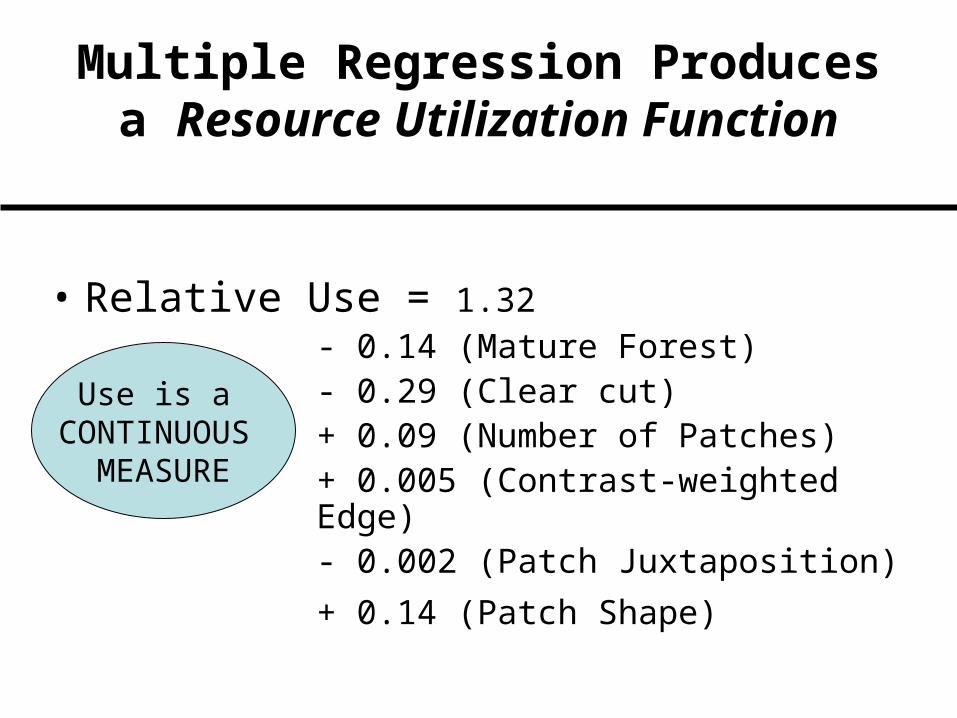
Multiple Regression Produces a Resource Utilization Function

• Relative Use = 1.32- 0.14 (Mature Forest)- 0.29 (Clear cut)+ 0.09 (Number of Patches)+ 0.005 (Contrast-weighted Edge)- 0.002 (Patch Juxtaposition)

+ 0.14 (Patch Shape)

Use is a CONTINUOUS

MEASURE

Relative Importance of Resources at the Population Level (n = 25)

 

Resource Attribute Mean

Standardized

95%

Confidence Interval

P

(

# of jays with use significantly

associated with attribute

+ -

Number of Patches +0.11* -0.57 – 0.28 0.19 14* 9

Contrast-weighted Edge +0.06* -0.13 – 0.26 0.50 10* 9

Mature Forest -0.05 -0.18 – 0.08 0.45 12 8

Clear cut -0.04 -0.17 – 0.09 0.51 6 9

Interspersion – Juxtaposition

-0.01* -0.14 – 0.16 0.87 11 8*

Patch Shape Index +0.01* -0.11 – 0.14 0.84 9* 12

* Use in direction predicted if jays select for edgy, fragmented areas within their home range

Dec

reas

ing

Impo

rtan

ce

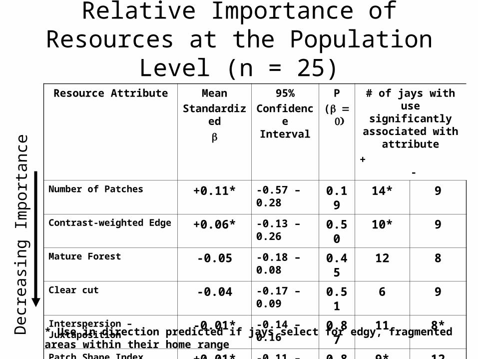
Relative Importance of Resources at the Population Level (n = 25)

 

Resource Attribute Mean

Standardized

95%

Confidence Interval

P

(

# of jays with use significantly

associated with attribute

+ -

Number of Patches +0.11* -0.57 – 0.28 0.19 14* 9

Contrast-weighted Edge +0.06* -0.13 – 0.26 0.50 10* 9

Mature Forest -0.05 -0.18 – 0.08 0.45 12 8

Clear cut -0.04 -0.17 – 0.09 0.51 6 9

Interspersion – Juxtaposition

-0.01* -0.14 – 0.16 0.87 11 8*

Patch Shape Index +0.01* -0.11 – 0.14 0.84 9* 12

* Use in direction predicted if jays select for edgy, fragmented areas within their home range

Dec

reas

ing

Impo

rtan

ce

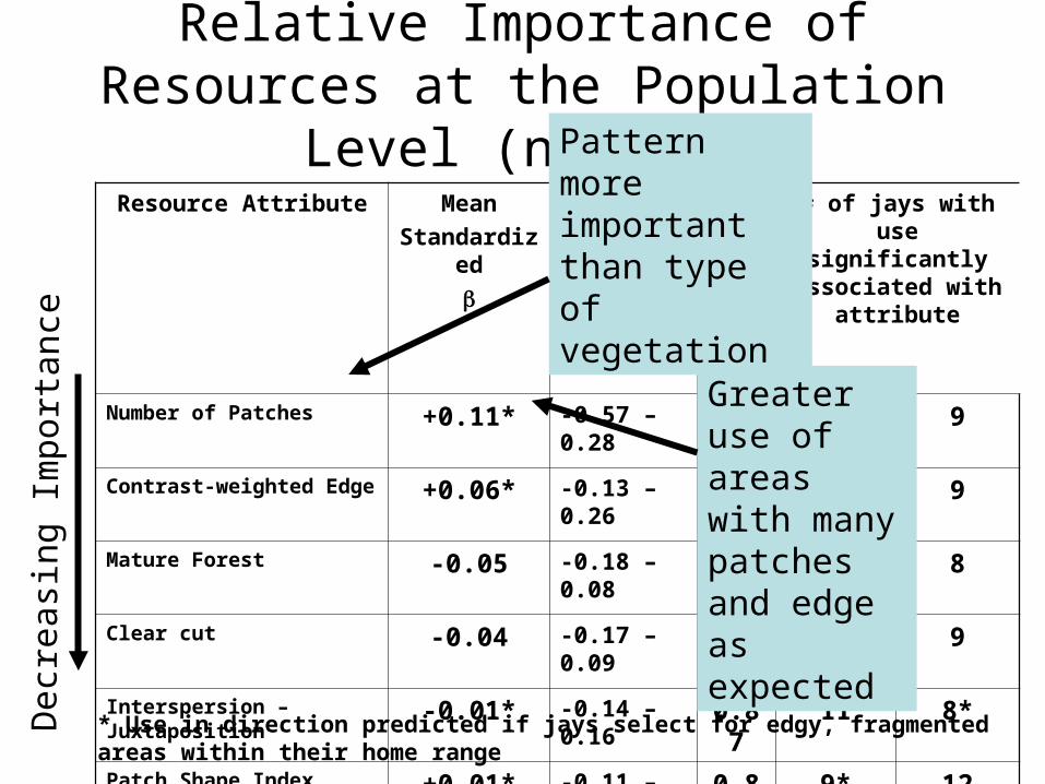
Greater use of areas with many patches and edge as expected

Pattern more important than type of vegetation

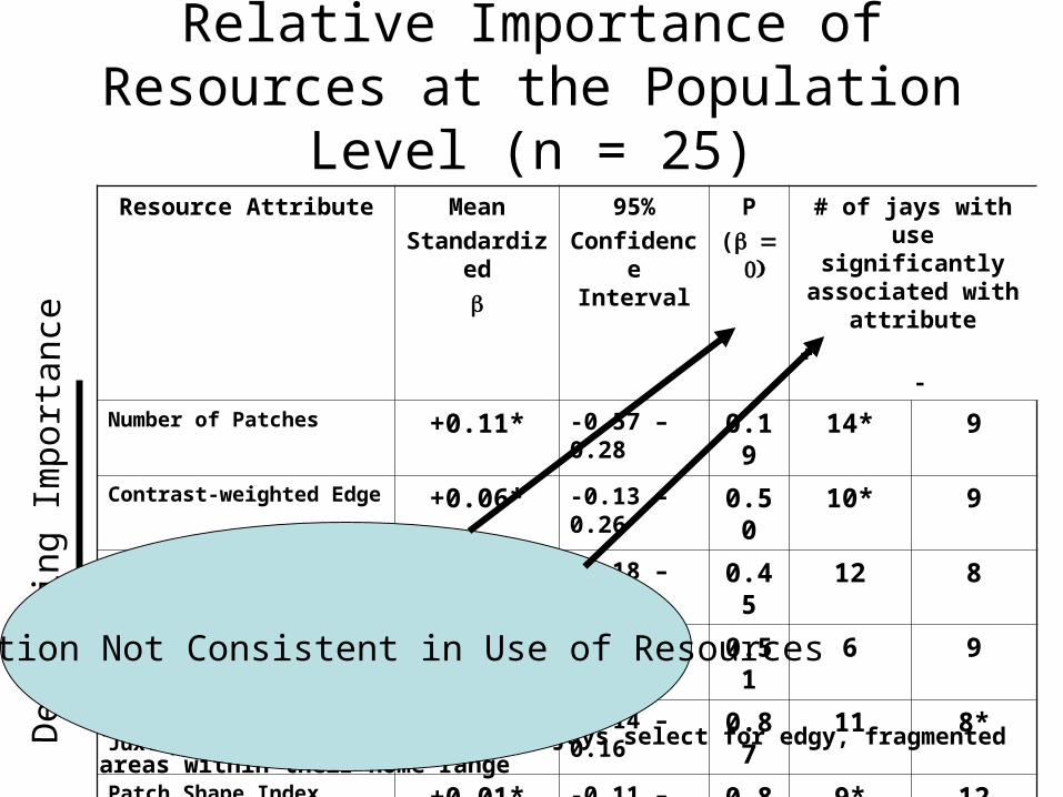
Relative Importance of Resources at the Population Level (n = 25)

 

Resource Attribute Mean

Standardized

95%

Confidence Interval

P

(

# of jays with use significantly

associated with attribute

+ -

Number of Patches +0.11* -0.57 – 0.28 0.19 14* 9

Contrast-weighted Edge +0.06* -0.13 – 0.26 0.50 10* 9

Mature Forest -0.05 -0.18 – 0.08 0.45 12 8

Clear cut -0.04 -0.17 – 0.09 0.51 6 9

Interspersion – Juxtaposition

-0.01* -0.14 – 0.16 0.87 11 8*

Patch Shape Index +0.01* -0.11 – 0.14 0.84 9* 12

* Use in direction predicted if jays select for edgy, fragmented areas within their home range

Dec

reas

ing

Impo

rtan

ce

Population Not Consistent in Use of Resources

Correlates of s Can Indicate Why Effects Are Not Greater

• Use of contrast-weighted edges is related to landscape shape index (P=0.03) and proximity to human activity (P=0.04)– >50% of variation

unaccounted for• Behaviorally-specific

use areas?

Rel

ativ

e U

se ()

of

Edg

e

<1Km >5Km

Proximity to Humans

N=10

N=15

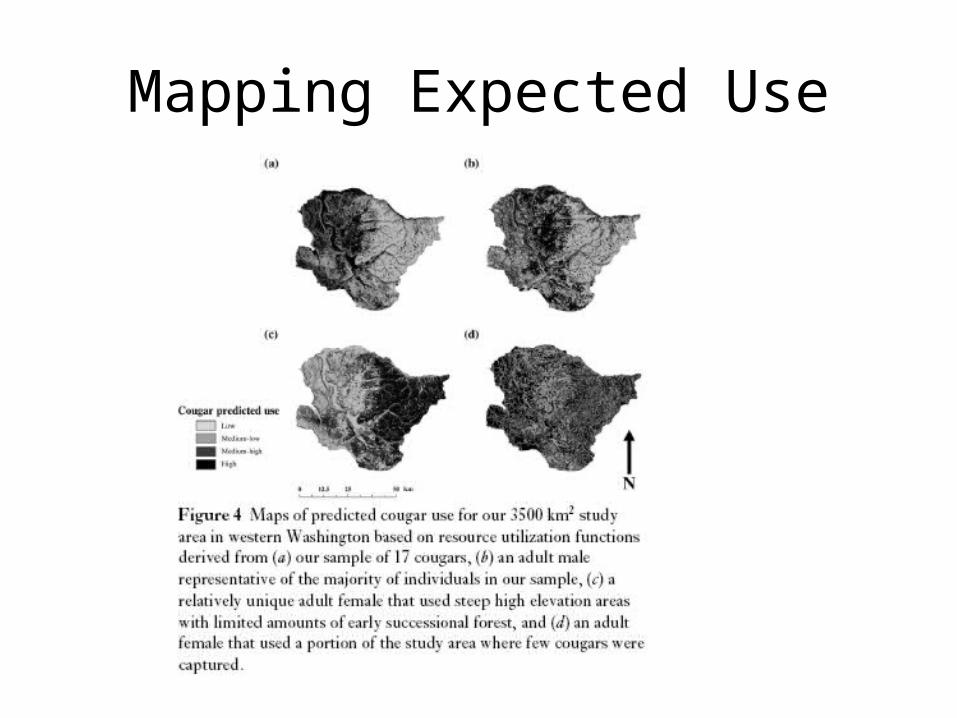
Mapping Expected Use

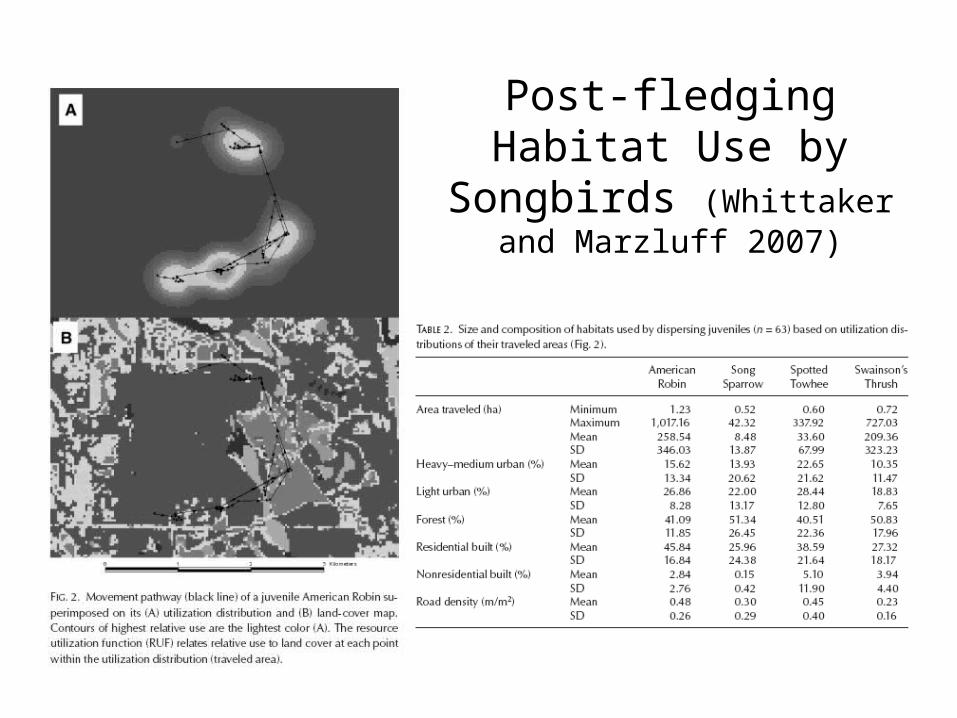
Post-fledging Habitat Use by Songbirds

(Whittaker and Marzluff 2007)

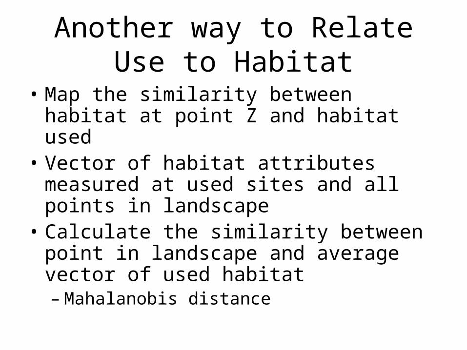
Another way to Relate Use to Habitat

• Map the similarity between habitat at point Z and habitat used

• Vector of habitat attributes measured at used sites and all points in landscape

• Calculate the similarity between point in landscape and average vector of used habitat– Mahalanobis distance

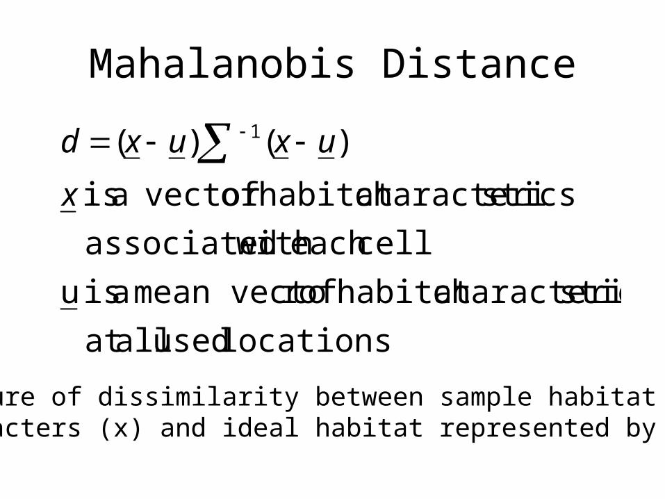
Mahalanobis Distance

locations used allat

sticscharacterihabitat ofr mean vecto a is u

celleach with associated

sticscharacterihabitat of vector a is

)()( 1

x

uxuxd

Measure of dissimilarity between sample habitat characters (x) and ideal habitat represented by u.

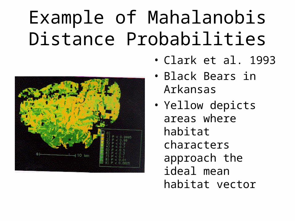
Example of Mahalanobis Distance Probabilities

• Clark et al. 1993• Black Bears in

Arkansas• Yellow depicts areas

where habitat characters approach the ideal mean habitat vector

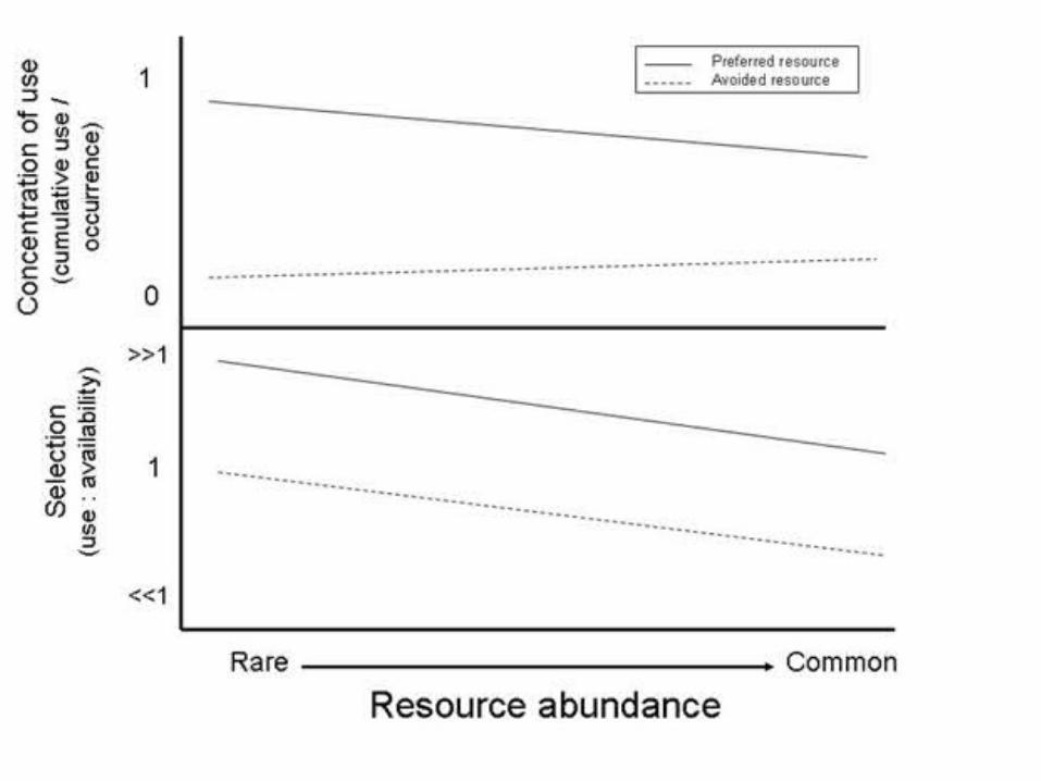
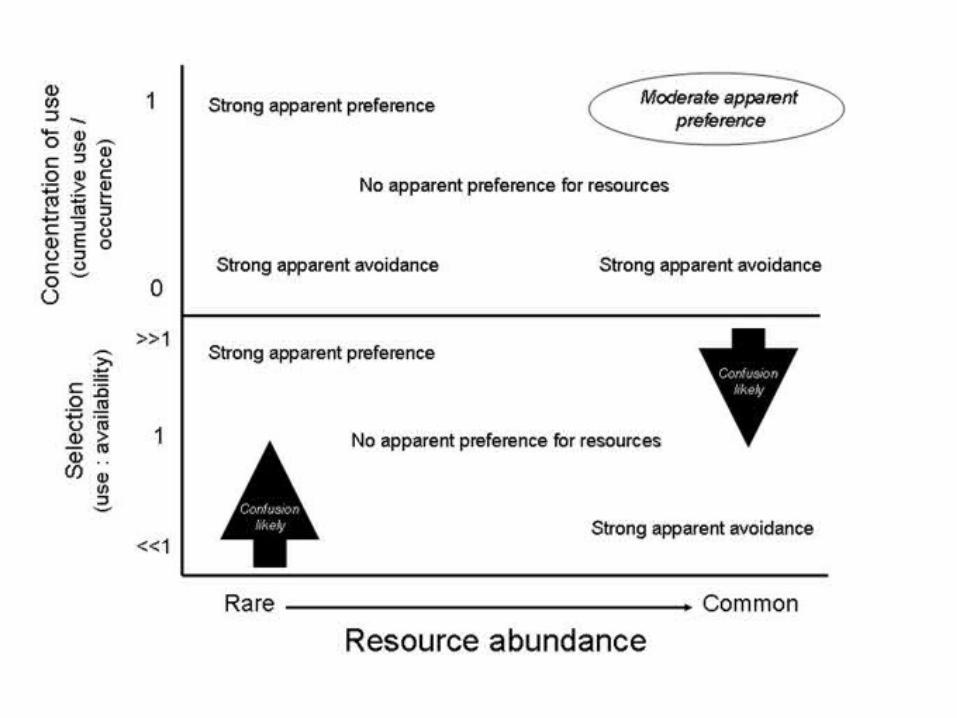
Scale and Our Perception of Availability

• Your insights and conclusions about resource selection are dependent upon your definition of resource availability– Availability in one sense defines the level in

the ordered selection hierarchy • You define available as habitat within the home

range or within the western US, etc.

• But the point is—the investigator defines availability

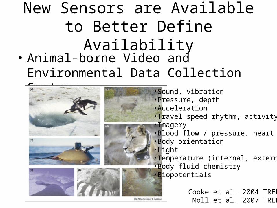
New Sensors are Available to Better Define Availability

• Animal-borne Video and Environmental Data Collection Systems

Cooke et al. 2004 TREE Moll et al. 2007 TREE

•Sound, vibration•Pressure, depth•Acceleration•Travel speed rhythm, activity•Imagery•Blood flow / pressure, heart rate•Body orientation•Light•Temperature (internal, external)•Body fluid chemistry•Biopotentials

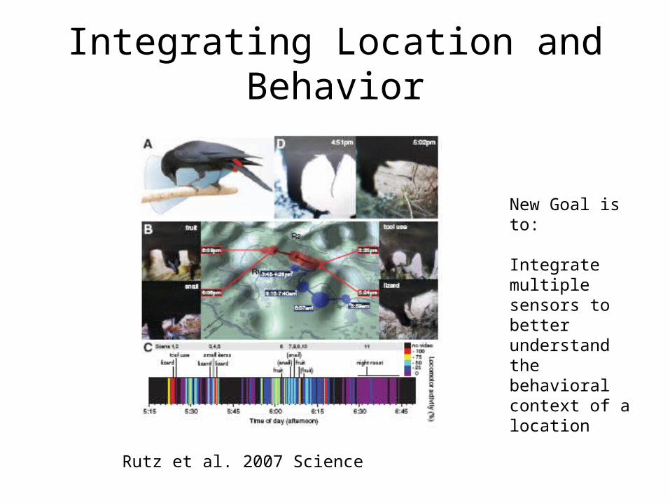
Integrating Location and Behavior

Rutz et al. 2007 Science

New Goal is to:

Integrate multiple sensors to better understand the behavioral context of a location

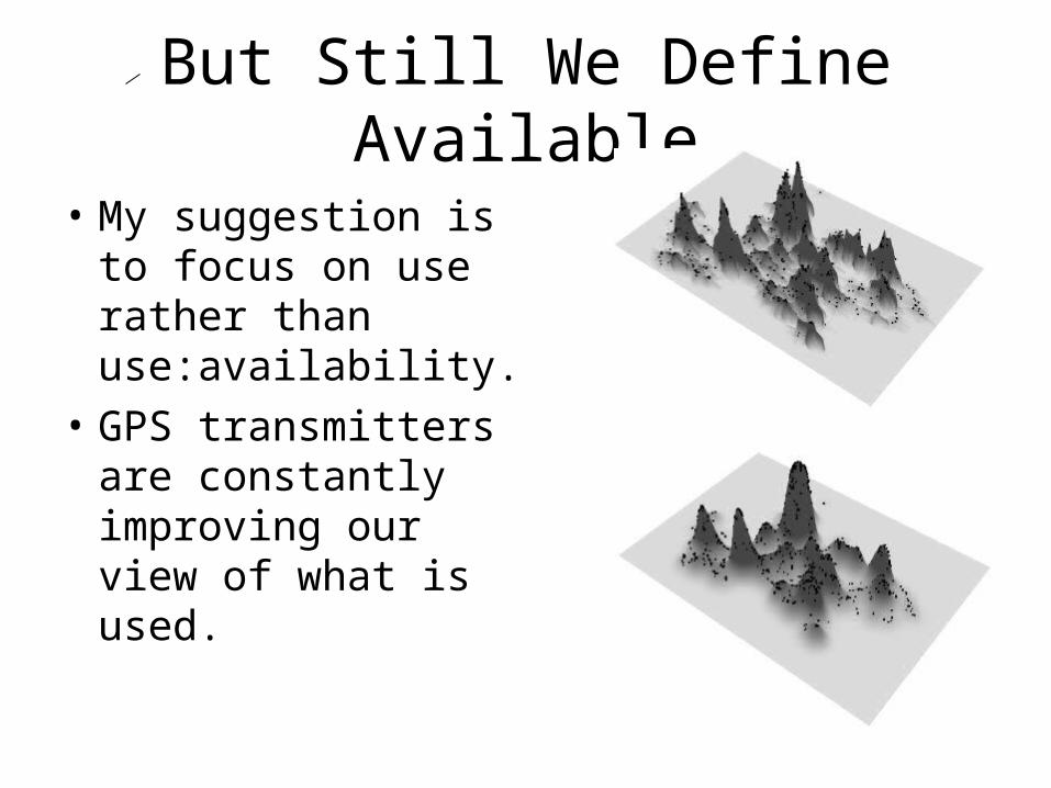
But Still We Define Available

• My suggestion is to focus on use rather than use:availability.

• GPS transmitters are constantly improving our view of what is used.

References• Wiens, JA, Van Horne, B., and BR Noon. 2002. Integrating landscape structure and scale into natural resource management. Pp. 23-67. In J. Liu

and WW Taylor, eds. Integrating landscape ecology into natural resource management. Cambridge University Press. Cambridge, UK• Brennen, JM, Bender, DJ, Contreras, TA, and L Fahrig. 2002. Focal patch landscape studies for wildlife management: optimizing sampling effort

across scales. Pp. 68-91. In J. Liu and WW Taylor, eds. Integrating landscape ecology into natural resource management. Cambridge University Press. Cambridge, UK

• Finn, SP, JM Marzluff, and DE Varland. 2002. Effects of landscape and local habitat attributes on northern goshawk site occupancy in western Washington. Forest Science 48:427-436.

• Finn, SP, DE Varland, and JM Marzluff. 2003.• Cody, ML. (ed.). 1985. Habitat selection in birds. Academic Press, San Diego, CA.• Fretwell, SD and Lucas, HL, Jr. 1969. On territorial behavior and other factors influencing habitat distribution in birds. Acta Biotheoret. 19:16-36.• Hilden, O. 1965. Habitat selection in birds. Annales Zoologici Fennici 2:53-75.• James, FC. 1971. Ordinations of habitat relationships among breeding birds. Wilson Bull. 83:215-236.• Klomp, H. 1954. De terreinkeus van de Kievit, Vanellus vanellus (L.). Ardea 42:1-139.• Klopfer, PH and JP Hailman. 1965. Habitat selection in birds. Advances in the Study of Behavior 1:279-303.• Klopfer, PH and JU Ganzhorn. 1985. Habitat selection: behavioral aspects. Pp. 435-453. In. M.L. Cody, ed. Habitat selection in birds. Academic

Press, San Diego, CA. • Partridge, L. 1978. Habitat selection. Pp. 351-376. In. J.R. Krebs and N. B. Davies, eds. Behavioural Ecology, an evolutionary approach. Sinauer.

Sunderland, MA.• Verner, J. 1975. Avian behavior and habitat management. Pp. 39-54. in Procedings of the Symposium on Management of Forest and Range

Habitats for Nongame Birds, Tuscon, AZ. May 6-9 1975.• Wiens, JA. 1972. Anuran habitat selection: early experience and substrate selection in Rana cascadae tadpoles. Animal Behaviour 20:218-220.• Wiens, JA. 1985. Habitat selection in variable environments: shrub-steppe birds. Pp. 227-251 In. M.L. Cody, ed. Habitat selection in birds. Academic

Press, San Diego, CA. • Wiens, JA. and JT. Rotenberry. 1981. Habitat associations and community structure of birds in shrubsteppe environments. Ecological Monographs

51:21-41.• Storch, I. 1997. The importance of scale in habitat conservation for an endangered species: the Capercaillie in central Europe. Pp. 310-330. In. JA

Bissonette, ed. Wildlife and landscape ecology. Springer. New York.• Bissonette, JA, DG Harrison, DC Hargis, and TG Chapin. 1997. The influence of spatial scale and scale-sensitive properties in habitat selection by

American marten. Pp. 368-385. In. JA Bissonette, ed. Wildlife and landscape ecology. Springer. New York.• Krausman, PR. 1997. The influence of landscape scale on the management of desert bighorn sheep. Pp. 349-367.. In. JA Bissonette, ed. Wildlife

and landscape ecology. Springer. New York.• Matthysen E. and D. Currie. 1996. habitat fragmentation reduces disperser success in juvenile nuthatches. Sitta europaea: evidence from patterns

of territory establishment. Ecography 19:72-76.• Johnson, D. H. 1980. The comparison of usage and availability measurements for evaluating resource preference. Ecology 61:65-71.• Rutz, C. et al. 2007. Video cameras on wild birds. Science 318:765.• Moll, R. J. et al. 2007. A new “view” of ecology and conservation through animal-borne video systems. Trends in Ecology and Evolution 22:660-668.• Cook, S. J. et al. 2004. Biotelemetry: a mechanistic approach to ecology. Trends in Ecology and Evolution 19:334-343.