Embed Size (px)
Citation preview
Laboratoire de l’Informatique du Parallélisme
École Normale Supérieure de LyonUnité Mixte de Recherche CNRS-INRIA-ENS LYON-UCBL no 5668
Resource Allocation using Virtual Clusters
Henri Casanova ,David Schanzenbach ,Mark Stillwell ,Frederic Vivien
October 2008
Research Report No 2008-33
École Normale Supérieure de Lyon46 Allée d’Italie, 69364 Lyon Cedex 07, France
Téléphone : +33(0)4.72.72.80.37Télécopieur : +33(0)4.72.72.80.80
Adresse électronique : [email protected]
Resource Allocation using Virtual Clusters
Henri Casanova , David Schanzenbach , Mark Stillwell , Frederic Vivien
October 2008
AbstractIn this report we demonstrate the potential utility of resource allocationmanagement systems that use virtual machine technology for sharingparallel computing resources among competing jobs. We formalize theresource allocation problem with a number of underlying assumptions,determine its complexity, propose several heuristic algorithms to findnear-optimal solutions, and evaluate these algorithms in simulation. Wefind that among our algorithms one is very efficient and also leads to thebest resource allocations. We then describe how our approach can bemade more general by removing several of the underlying assumptions.
Keywords: Virtualization, virtual cluster, scheduling, resource management, fairness
ResumeDans ce rapport nous montrons l’utilite potentielle des systemes de ges-tion de ressources qui utilisent la technologie des machines virtuellespour partager, entre un ensemble de taches, des ressources de calculparalleles. Nous formalisons le probleme d’allocation de ressources aumoyen d’hypotheses simplificatrices, nous determinons sa complexite,nous proposons plusieurs heuristiques pour trouver des solutions appro-chees, et nous evaluons ces solutions au moyen de simulations. Nous eta-blissons qu’une de nos solutions est tres efficace et mene a la meilleureallocation des ressources. Finalement, nous montrons comment notreapproche peut-etre generalisee en eliminant certaines de nos hypothesessimplificatrices.
Mots-cles: Virtualisation, cluster virtuel, ordonnancement, gestion des ressources, equite

Resource Allocation using Virtual Clusters 1
1 Introduction
The use of commodity clusters has become mainstream for high-performance computing appli-cations, with more than 80% of today’s fastest supercomputers being clusters [49]. Large-scaledata processing [23, 39, 33] and service hosting [22, 4] are also common applications. Theseclusters represent significant equipment and infrastructure investment, and having a high rateof utilization is key for justifying their ongoing costs (hardware, power, cooling, staff) [24,50].There is therefore a strong incentive to share these clusters among a large number of appli-cations and users.
The sharing of compute resources among competing instances of applications, or jobs,within a single system has been supported by operating systems for decades via time-sharing.Time-sharing is implemented with rapid context-switching and is motivated by a need forinteractivity. A fundamental assumption is that there is no or little a-priori knowledge re-garding the expected workload, including expected durations of running processes. This isvery different from the current way in which clusters are shared. Typically, users request somefraction of a cluster for a specified duration. In the traditional high-performance computingarena, the ubiquitous approach is to use“batch scheduling”, by which jobs are placed in queueswaiting to gain exclusive access to a subset of the platform for a bounded amount of time. Inservice hosting or cloud environments, the approach is to allow users to lease “virtual slices”of physical resources, enabled by virtual machine technology. The latter approach has sev-eral advantages, including O/S customization and interactive execution. In general resourcesharing among competing jobs is difficult because jobs have different resource requirements(amount of resources, time needed) and because the system cannot accommodate all jobs atonce.
An important observation is that both resource allocation approaches mentioned abovedole out integral subsets of the resources, or allocations (e.g., 10 physical nodes, 20 virtualslices), to jobs. Furthermore, in the case of batch scheduling, these subsets cannot changethroughout application execution. This is a problem because most applications do not useall resources allocated to them at all times. It would then be useful to be able to decreaseand increase application allocations on-the-fly (e.g., by removing and adding more physicalcluster nodes or virtual slices during execution). Such application are termed “malleable” inthe literature. While solutions have been studied to implement and to schedule malleableapplications [46,12,25,51,52], it is often difficult to make sensible malleability decisions at theapplication level. Furthermore, many applications are used as-is, with no desire or possibilityto re-engineer them to be malleable. As a result sensible and automated malleability is rare inreal-world applications. This is perhaps also due to the fact that production batch schedulingenvironment do not provide mechanisms for dynamically increasing or decreasing allocations.By contrast, in service hosting or cloud environments, acquiring and relinquishing virtualslices is straightforward and can be implemented via simple mechanisms. This provides addedmotivation to engineer applications to be malleable in those environments.
Regardless, an application that uses only 80% of a cluster node or of a virtual slice wouldneed to relinquish only 20% of this resources. However, current resource allocation schemesallocate integral numbers of resources (whether these are physical cluster nodes or virtualslices). Consequently, many applications are denied access to resources, or delayed, in spiteof cluster resources not being fully utilized by the applications that are currently executing,which hinders both application throughput and cluster utilization.
The second limitation of current resource allocation schemes stems from the fact that
2 H. Casanova , D. Schanzenbach , M. Stillwell , F. Vivien
resource allocation with integral allocations is difficult from a theoretical perspective [10].Resource allocation problems are defined formally as the optimizations of well-defined objec-tive functions. Due to the difficulty (i.e., NP-hardness) of resource allocation for optimizingan objective function, in the real-world no such objective function is optimized. For instance,batch schedulers instead provide a myriad of configuration parameters by which a cluster ad-ministrator can tune the scheduling behavior according to ad-hoc rules of thumb. As a result,it has been noted that there is a sharp disconnect between the desires of users (low applicationturn-around time, fairness) and the schedules computed by batch schedulers [44,26]. It turnsout that cluster administrators often attempt to maximize cluster utilization. But recall that,paradoxically, current resource allocation schemes inherently hinder cluster utilization!
A notable finding in the theoretical literature is that with job preemption and/or migra-tion there is more flexibility for resource allocation. In this case certain resource allocationproblems become (more) tractable or approximable [6, 44,27,35,11]. Unfortunately, preemp-tion and migration are rarely used on production parallel platforms. The gang scheduling [38]approach allows entire parallel jobs to be context-switched in a synchronous fashion. Unfortu-nately, a known problem with this approach is the overhead of coordinated context switchingon a parallel platform. Another problem is the memory pressure due to the fact that clus-ter applications often use large amounts of memory, thus leading to costly swapping betweenmemory and disk [9]. Therefore, while flexibility in resource allocations is desirable for solvingresource allocation problems, affording this flexibility has not been successfully accomplishedin production systems.
In this paper we argue that both limitations of current resource allocation schemes, namely,reduced utilization and lack of an objective function, can be addressed simultaneously viafractional and dynamic resource allocations enabled by state-of-the-art virtual machine (VM)technology. Indeed, applications running in VM instances can be monitored so as to discovertheir resource needs, and their resource allocations can be modified dynamically (by appro-priately throttling resource consumption and/or by migrating VM instances). Furthermore,recent VM technology advances make the above possible with low overhead. Therefore, it ispossible to use this technology for resource allocation based on the optimization of sensibleobjective functions, e.g., ones that capture notions of performance and fairness.
Our contributions are:
• We formalize a general resource allocation problem based on a number of assumptionsregarding the platform, the workload, and the underlying VM technology;
• We establish the complexity of the problem and propose algorithms to solve it;
• We evaluate our proposed algorithms in simulation and identify an algorithm that isvery efficient and leads to better resource allocations than its competitors;
• We validate our assumptions regarding the capabilities of VM technology;
• We discuss how some of our other assumptions can be removed and our approachadapted.
This paper is organized as follows. In Section 2 we define and formalize our target prob-lem, we list our assumptions for the base problem, and we establish its NP-hardness. InSection 3 we propose algorithms for solving the base problem and evaluate these algorithmsin simulation in Section 4. Sections 5 and 6 study the resource sharing problem with relaxed
Resource Allocation using Virtual Clusters 3
VM Monitor
VM Monitor VM Monitor VM Monitor
VM Monitor VM Monitor VM Monitor
VM instance for VC #1
VM instance for VC #2
VM instance for VC #3
VC RequestsResourceAllocator
VM
Managem
ent System
VM Monitor VM Monitor VM Monitor
VM Monitor VM Monitor
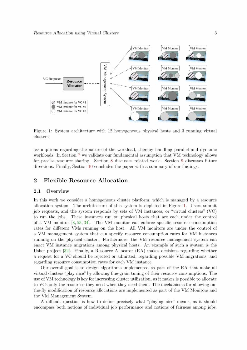
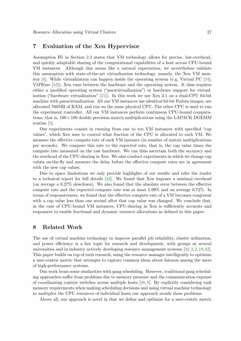
Figure 1: System architecture with 12 homogeneous physical hosts and 3 running virtualclusters.
assumptions regarding the nature of the workload, thereby handling parallel and dynamicworkloads. In Section 7 we validate our fundamental assumption that VM technology allowsfor precise resource sharing. Section 8 discusses related work. Section 9 discusses futuredirections. Finally, Section 10 concludes the paper with a summary of our findings.
2 Flexible Resource Allocation
2.1 Overview
In this work we consider a homogeneous cluster platform, which is managed by a resourceallocation system. The architecture of this system is depicted in Figure 1. Users submitjob requests, and the system responds by sets of VM instances, or “virtual clusters” (VC)to run the jobs. These instances run on physical hosts that are each under the controlof a VM monitor [8, 53, 34]. The VM monitor can enforce specific resource consumptionrates for different VMs running on the host. All VM monitors are under the control ofa VM management system that can specify resource consumption rates for VM instancesrunning on the physical cluster. Furthermore, the VM resource management system canenact VM instance migrations among physical hosts. An example of such a system is theUsher project [32]. Finally, a Resource Allocator (RA) makes decisions regarding whethera request for a VC should be rejected or admitted, regarding possible VM migrations, andregarding resource consumption rates for each VM instance.
Our overall goal is to design algorithms implemented as part of the RA that make allvirtual clusters “play nice” by allowing fine-grain tuning of their resource consumptions. Theuse of VM technology is key for increasing cluster utilization, as it makes is possible to allocateto VCs only the resources they need when they need them. The mechanisms for allowing on-the-fly modification of resource allocations are implemented as part of the VM Monitors andthe VM Management System.
A difficult question is how to define precisely what “playing nice” means, as it shouldencompass both notions of individual job performance and notions of fairness among jobs.

4 H. Casanova , D. Schanzenbach , M. Stillwell , F. Vivien
We address this issue by defining a performance metric that encompasses both these notionsand that can be used to value resource allocations. The RA may be configured with the goal ofoptimizing this metric but at the same time ensuring that the metric across the jobs is abovesome threshold (for instance by rejecting requests for new virtual clusters). More generally,a key aspect of our approach is that it can be combined with resource management andaccounting techniques. For instance, it is straightforward to add notions of user priorities,of resource allocation quotas, of resource allocation guarantees, or of coordinated resourceallocations to VMs belonging to the same VC. Furthermore, the RA can reject or delay VCrequests if the performance metric is below some acceptable level, to be defined by clusteradministrators.
2.2 Assumptions
We first consider the resource sharing problem using the following six assumptions regardingthe workload, the physical platform, and the VM technology in use:
(H1) Jobs are CPU-bound and require a given amount of memory to be able to run;
(H2) Job computational power needs and memory requirements are known;
(H3) Each job requires only one VM instance;
(H4) The workload is static, meaning jobs have constant resource requirements; furthermore,no job enters or leaves the system;
(H5) VM technology allows for precise, low-overhead, and quickly adaptable sharing of thecomputational capabilities of a host across CPU-bound VM instances.
These assumptions are very stringent, but provide a good framework to formalize ourresource allocation problem (and to prove that it is difficult even with these assumptions). Werelax assumption H3 in Section 5, that is, we consider parallel jobs. Assumption H4 amountsto assuming that jobs have no time horizons, i.e., that they run forever with unchangingrequirements. In practice, the resource allocation may need to be modified when the workloadchanges (e.g., when a new job arrives, when a job terminates, when a job starts needingmore/fewer resources). In Section 6 we relax assumption H4 and extend our approach toallow allocation adaptation. We validate assumption H5 in Section 7. We leave relaxing H1and H2 for future work, and discuss the involved challenges in Section 10.
2.3 Problem Statement
We call the resource allocation problem described in the previous section VCSched anddefine it here formally. Consider H > 0 identical physical hosts and J > 0 jobs. For job i,i = 1, . . . , J , let αi be the (average) fraction of a host’s computational capability utilized bythe job if alone on a physical host, 0 ≤ αi ≤ 1. (Alternatively, this fraction could be specifieda-priori by the user who submitted/launched job i.) Let mi be the maximum fraction of ahost’s memory needed by job i, 0 ≤ mi ≤ 1. Let αij be the fraction of the computationalcapability of host j, j = 1, . . . ,H, allocated to job i, i = 1, . . . , J . We have 0 ≤ αij ≤ 1. Ifαij is constrained to be an integer, that is either 0 or 1, then the model is that of schedulingwith exclusive access to resources. If, instead, αij is allowed to take rational values between0 and 1, then resource allocations can be fractional and thus more fine-grain.

Resource Allocation using Virtual Clusters 5
Constraints – We can write a few constraints due to resource limitations. We have
∀jJ∑i=1
αij ≤ 1 ,
which expresses the fact that the total CPU fraction allocated to jobs on any single host maynot exceed 100%. Also, a job should not be allocated more resource than it can use:
∀iH∑j=1
αij ≤ αi ,
Similarly,
∀jJ∑i=1
dαijemi ≤ 1 , (1)
since at most the entire memory on a host may be used.With assumption H3, a job requires only one VM instance. Furthermore, as justified
hereafter, we assume that we do not use migration and that a job can be allocated to a singlehost. Therefore, we write the following constraints:
∀iH∑j=1
dαije = 1 , (2)
which state that for all i only one of the αij values is non-zero.
Objective function – We wish to optimize a performance metric that encompasses bothnotions of performance and of fairness, in an attempt at designing the scheduler from thestart with a user-centric metric in mind (unlike, for instance, current batch schedulers). In thetraditional parallel job scheduling literature, the metric commonly acknowledged as being agood measure for both performance and fairness is the stretch (also called“slowdown”) [10,16].The stretch of a job is defined as the job’s turn-around time divided by the turn-around timethat would have been achieved had the job been alone in the system.
This metric cannot be applied directly in our context because jobs have no time horizons.So, instead, we use a new metric, which we call the yield and which we define for job i as∑j αij/αi. The yield of a job represents the fraction of its maximum achievable compute
rate that is achieved (recall that for each i only one of the αij is non-zero). A yield of 1means that the job consumes compute resources at its peak rate. We can now define problemVCSched as maximizing the minimum yield in an attempt at optimizing both performanceand fairness (similar in spirit to minimizing the maximum stretch [10, 27]). Note that wecould easily maximize the average yield instead, but we may then decrease the fairness of theresource allocation across jobs as average metrics are starvation-prone [27]. Our approach isagnostic to the particular objective function (although some of our results hold only for linearobjective functions). For instance, other ways in which the stretch can be optimized havebeen proposed [7] and could be adapted for our yield metric.
6 H. Casanova , D. Schanzenbach , M. Stillwell , F. Vivien
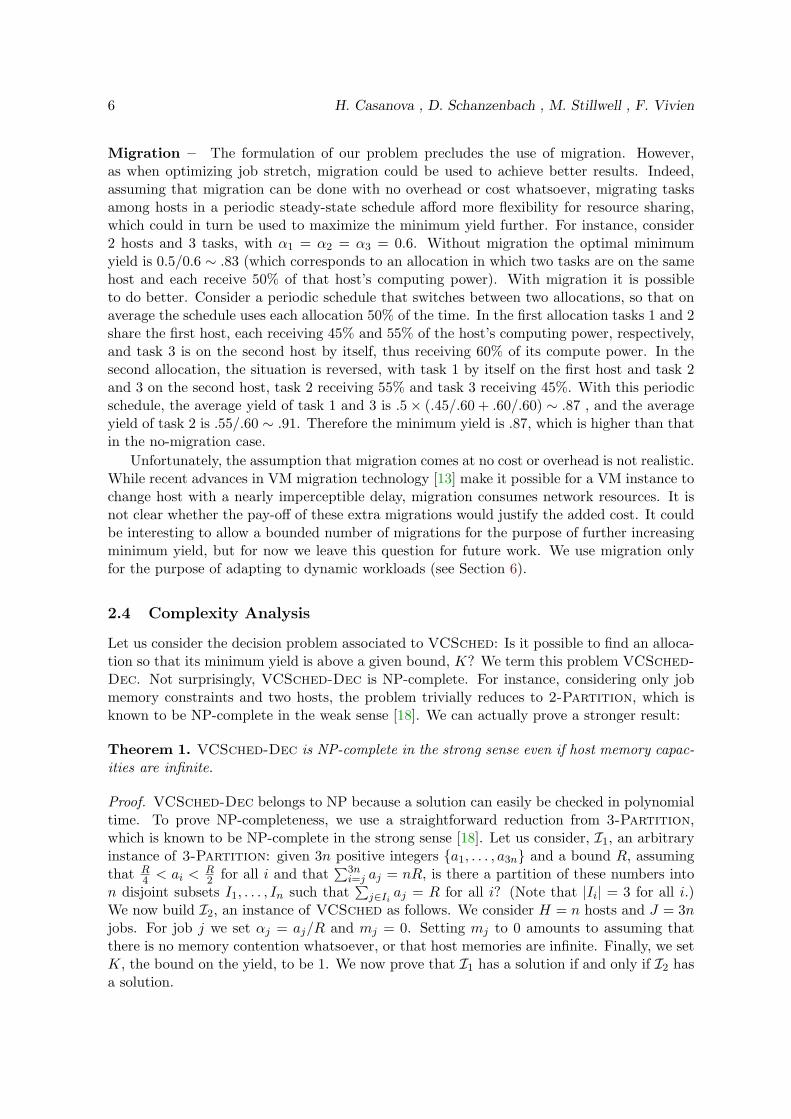
Migration – The formulation of our problem precludes the use of migration. However,as when optimizing job stretch, migration could be used to achieve better results. Indeed,assuming that migration can be done with no overhead or cost whatsoever, migrating tasksamong hosts in a periodic steady-state schedule afford more flexibility for resource sharing,which could in turn be used to maximize the minimum yield further. For instance, consider2 hosts and 3 tasks, with α1 = α2 = α3 = 0.6. Without migration the optimal minimumyield is 0.5/0.6 ∼ .83 (which corresponds to an allocation in which two tasks are on the samehost and each receive 50% of that host’s computing power). With migration it is possibleto do better. Consider a periodic schedule that switches between two allocations, so that onaverage the schedule uses each allocation 50% of the time. In the first allocation tasks 1 and 2share the first host, each receiving 45% and 55% of the host’s computing power, respectively,and task 3 is on the second host by itself, thus receiving 60% of its compute power. In thesecond allocation, the situation is reversed, with task 1 by itself on the first host and task 2and 3 on the second host, task 2 receiving 55% and task 3 receiving 45%. With this periodicschedule, the average yield of task 1 and 3 is .5× (.45/.60 + .60/.60) ∼ .87 , and the averageyield of task 2 is .55/.60 ∼ .91. Therefore the minimum yield is .87, which is higher than thatin the no-migration case.
Unfortunately, the assumption that migration comes at no cost or overhead is not realistic.While recent advances in VM migration technology [13] make it possible for a VM instance tochange host with a nearly imperceptible delay, migration consumes network resources. It isnot clear whether the pay-off of these extra migrations would justify the added cost. It couldbe interesting to allow a bounded number of migrations for the purpose of further increasingminimum yield, but for now we leave this question for future work. We use migration onlyfor the purpose of adapting to dynamic workloads (see Section 6).
2.4 Complexity Analysis
Let us consider the decision problem associated to VCSched: Is it possible to find an alloca-tion so that its minimum yield is above a given bound, K? We term this problem VCSched-Dec. Not surprisingly, VCSched-Dec is NP-complete. For instance, considering only jobmemory constraints and two hosts, the problem trivially reduces to 2-Partition, which isknown to be NP-complete in the weak sense [18]. We can actually prove a stronger result:
Theorem 1. VCSched-Dec is NP-complete in the strong sense even if host memory capac-ities are infinite.
Proof. VCSched-Dec belongs to NP because a solution can easily be checked in polynomialtime. To prove NP-completeness, we use a straightforward reduction from 3-Partition,which is known to be NP-complete in the strong sense [18]. Let us consider, I1, an arbitraryinstance of 3-Partition: given 3n positive integers {a1, . . . , a3n} and a bound R, assumingthat R
4 < ai <R2 for all i and that
∑3ni=j aj = nR, is there a partition of these numbers into
n disjoint subsets I1, . . . , In such that∑j∈Ii aj = R for all i? (Note that |Ii| = 3 for all i.)
We now build I2, an instance of VCSched as follows. We consider H = n hosts and J = 3njobs. For job j we set αj = aj/R and mj = 0. Setting mj to 0 amounts to assuming thatthere is no memory contention whatsoever, or that host memories are infinite. Finally, we setK, the bound on the yield, to be 1. We now prove that I1 has a solution if and only if I2 hasa solution.

Resource Allocation using Virtual Clusters 7
Let us assume that I1 has a solution. For each job j, we assign it to host i if j ∈ Ii, and wegive it all the compute power it needs (αji = aj/R). This is possible because
∑j∈Ii aj = R,
which implies that∑j∈Ii αji = R/R ≤ 1. In other terms, the computational capacity of each
host is not exceeded. As a result, each job has a yield of K = 1 and we have built a solutionto I2.
Let us now assume that I2 has a solution. Then, for each job j there exists a unique ijsuch that αjij = αj , and such that αji = 0 for i 6= ij (i.e., job j is allocated to host ij). Letus define Ii = {j|ij = i}. By this definition, the Ii sets are disjoint and form a partition of{1, . . . , 3n}.
To ensure that each processor’s compute capability is not exceeded, we must have∑j∈Ii αj ≤
1 for all i. However, by construction of I2,∑3nj=1 αj = n. Therefore, since the Ii sets form
a partition of {1, . . . , 3n},∑j∈Ii αj is exactly equal to 1 for all i. Indeed, if
∑j∈Ii1
αj werestrictly lower than 1 for some i1, then
∑j∈Ii2
αj would have to be greater than 1 for some i2,meaning that the computational capability of a host would be exceeded. Since αj = aj/R,we obtain
∑j∈Ii aj = R for all i. Sets Ii are thus a solution to I1, which concludes the proof.
2.5 Mixed-Integer Linear Program Formulation
It turns out that VCSched can be formulated as a mixed-integer linear program (MILP),that is an optimization problem with linear constraints and objective function, but with bothrational and integer variables. Among the constraints given in Section 2.3, the constraints inEq. 1 and Eq. 2 are non-linear. These constraints can easily be made linear by introducing abinary integer variables, eij , set to 1 if job i is allocated to resource j, and to 0 otherwise. Wecan then rewrite the constraints in Section 2.3 as follows, with i = 1, . . . , J and j = 1, . . . ,H:
∀i, j eij ∈ N, (3)∀i, j αij ∈ Q, (4)∀i, j 0 ≤ eij ≤ 1, (5)∀i, j 0 ≤ αij ≤ eij , (6)∀i
∑Hj=1 eij = 1, (7)
∀j∑Ji=1 αij ≤ 1, (8)
∀j∑Ji=1 eijmi ≤ 1 (9)
∀i∑Hj=1 αij ≤ αi (10)
∀i∑Hj=1
αij
αi≥ Y (11)
Recall that mi and αi are constants that define the jobs. The objective is to maximize Y ,i.e., to maximize the minimum yield.
3 Algorithms for Solving VCSched
In this section we propose algorithms to solve VCSched, including exact and relaxed solutionsof the MILP in Section 2.5 as well as ad-hoc heuristics. We also give a generally applicabletechnique to improve average yield further once the minimum yield has been maximized.

8 H. Casanova , D. Schanzenbach , M. Stillwell , F. Vivien
3.1 Exact and Relaxed Solutions
In general, solving a MILP requires exponential time and is only feasible for small probleminstances. We use a publicly available MILP solver, the Gnu Linear Programming Toolkit(GLPK), to compute the exact solution when the problem instance is small (i.e., few tasksand/or few hosts). We can also solve a relaxation of the MILP by assuming that all variablesare rational, converting the problem to a LP. In practice a rational linear program can besolved in polynomial time. However, the resulting solution may be infeasible (namely becauseit could spread a single job over multiple hosts due to non-binary eij values), but has twoimportant uses. First, the value of the objective function is an upper bound on what isachievable in practice, which is useful to evaluate the absolute performance of heuristics.Second, the rational solution may point the way toward a good feasible solution that iscomputed by rounding off the eij values to integer values judiciously, as discussed in the nextsection.
It turns out that we do not need a linear program solver to compute the optimal minimumyield for the relaxed program. Indeed, if the total of job memory requirement is not largerthan the total available memory (i.e., if
∑Ji=1mi ≤ H), then there is a solution to the relaxed
version of the problem and the achieved optimal minimum yield, Y (rat)opt , can be computed
easily:
Y(rat)opt = min{ H∑J
i=1 αi, 1}.
The above expression is an obvious upper bound on the maximum minimum yield. To showthat it is in fact the optimal, we simply need to exhibit an allocation that achieves thisobjective. A simple such allocation is:
∀i, j eij =1H
and αij =1HαiY
(rat)opt .
3.2 Algorithms Based on Relaxed Solutions
We propose two heuristics, RRND and RRNZ, that use a solution of the rational LP as abasis and then round-off rational eij value to attempt to produce a feasible solution, whichis a classical technique. In the previous section we have shown a solution for the LP; Un-fortunately, that solution has the undesirable property that it splits each job evenly acrossall hosts, meaning that all eij values are identical. Therefore it is a poor starting point forheuristics that attempt to round off eij values based on their magnitude. Therefore, we useGLPK to solve the relaxed MILP and use the produced solution as a starting point instead.Randomized Rounding (RRND) – This heuristic first solves the LP. Then, for each job i(taken in an arbitrary order), it allocates it to a random host using a probability distributionby which host j has probability eij of being selected. If the job cannot fit on the selected hostbecause of memory constraints, then that host’s probability of being selected is set to zeroand another attempt is made with the relative probabilities of the remaining hosts adjustedaccordingly. If no selection has been made and every host has zero probability of beingselected, then the heuristic fails. Such a probabilistic approach for rounding rational variablevalues into integer values has been used successfully in previous work [31].Randomized Rounding with No Zero probability (RRNZ) – This heuristic is a slightmodification of the RRND heuristic. One problem with RRND is that a job, i, may notfit (in terms of memory requirements) on any of the hosts, j, for which eij > 0, in which
Resource Allocation using Virtual Clusters 9
case the heuristic would fail to generate a solution. To remedy this problem, we set each eijvalue equal to zero in the solution of the relaxed MILP to ε instead, where ε << 1 (we usedε = 0.01). For those problem instances for which RRND provides a solution RRNZ shouldprovide nearly the same solution most of the time. But RRNZ should also provide a solutionto a some instances for which RRND fails, thus achieving a better success rate.
3.3 Greedy Algorithms
Greedy (GR) – This heuristic first goes through the list of jobs in arbitrary order. Foreach job the heuristic ranks the hosts according to their total computational load, that is, thetotal of the maximum computation requirements of all jobs already assigned to a host. Theheuristic then selects the first host, in non decreasing order of computational load, for whichan assignment of the current job to that host will satisfy the job’s memory requirements.Sorted-Task Greedy (SG) – This version of the greedy heuristic first sorts the jobs indescending order by their memory requirements before proceeding as in the standard greedyalgorithm. The idea is to place relatively large jobs while the system is still lightly loaded.Greedy with Backtracking (GB) – It is possible to modify the GR heuristic to add back-tracking. Clearly full-fledged backtracking would lead to 100% success rate for all instancesthat have a feasible solution, but it would also require potentially exponential time. One thusneeds methods to prune the search tree. We use a simple method, placing an arbitrary bound(500,000) on the number of job placement attempts. An alternate pruning technique wouldbe to restrict placement attempts to the top 25% candidate placements, but based on ourexperiments it is vastly inferior to using an arbitrary bound on job placement attempts.Sorted Greedy with Backtracking (SGB) – This version is a combination of SG and GB,i.e., tasks are sorted in descending order of memory requirement as in SG and backtrackingis used as in GB.
3.4 Multi-Capacity Bin Packing Algorithms
Resource allocation problems are often akin to bin packing problems, and VCSched is noexception. There are however two important differences between our problem and bin packing.First, our tasks resource requirements are dual, with both memory and CPU requirements.Second, our CPU requirements are not fixed but depend on the achieved yield. The firstdifference can be addressed by using “multi-capacity” bin packing heuristics. Two Multi-capacity bin packing heuristics were proposed in [28] for the general case of d-capacity binsand items, but in the d = 2 case these two algorithms turn out to be equivalent. The seconddifference can be addressed via a binary search on the yield value.
Consider an instance of VCSched and a fixed value of the yield, Y , that needs to beachieved. By fixing Y , each task has both a fixed memory requirement and a fixed CPUrequirement, both taking values between 0 and 1, making it possible to apply the algorithmin [28] directly.
Accordingly, one splits the tasks into two lists, with one list containing the tasks withhigher CPU requirements than memory requirements and the other containing the tasks withhigher memory requirements than CPU requirements. One then sorts each list. In [28] thelists are sorted according to the sum of the CPU and memory requirements.
Once the lists are sorted, one can start assigning tasks to the first host. Lists are alwaysscanned in order, searching for a task that can “fit” on the host, which for the sake of this

10 H. Casanova , D. Schanzenbach , M. Stillwell , F. Vivien
discussion we term a “possible task”. Initially one searches for a possible task in one andthen the other list, starting arbitrarily with any list. This task is then assigned to the host.Subsequently, one always searches for a possible task from the list that goes against thecurrent imbalance. For instance, say that the host’s available memory capacity is 50% andits available CPU capacity is 80%, based on tasks that have been assigned to it so far. Inthis case one would scan the list of tasks that have higher CPU requirements than memoryrequirements to find a possible task. If no such possible task is found, then one scans theother list to find a possible task. When no possible tasks are found in either list, one startsthis process again for the second host, and so on for all hosts. If all tasks can be assigned inthis manner on the available hosts, then resource allocation is successful. Otherwise resourceallocation fails.
The final yield must be between 0, representing failure, and the smaller of 1 or the totalcomputation capacity of all the hosts divided by the total computational requirements of allthe tasks. We arbitrarily choose to start at one-half of this value and perform a binary searchof possible minimum yield values, seeking to maximize minimum yield. Note that under somecircumstances the algorithm may fail to find a valid allocation at a given potential yield value,even though it would find one given a larger yield value. This type of failure condition is tobe expected when applying heuristics.
While the algorithm in [28] sorts each list by the sum of the memory and CPU require-ments, there are other likely sorting key candidates. For completeness we experiment with 8different options for sorting the lists, each resulting in a MCB (Multi-Capacity Bin Packing)algorithm. We describe all 8 options below:
• MCB1: memory + CPU, in ascending order;
• MCB2: max(memory,CPU) - min(memory,CPU), in ascending order;
• MCB3: max(memory,CPU) / min(memory,CPU), in ascending order;
• MCB4: max(memory,CPU), in ascending order;
• MCB5: memory + CPU, in descending order;
• MCB6: max(memory,CPU) - min(memory,CPU), in descending order.
• MCB7: max(memory,CPU) / min(memory,CPU), in descending order;
• MCB8: max(memory,CPU), in descending order;
3.5 Increasing Average Yield
While the objective function to be maximized for solving VCSched is the minimum yield,once an allocation that achieves this goal has been found there may be excess computationalresources available which would be wasted if not allocated. Let us call Y the maximizedminimum yield value computed by one of the aforementioned algorithms (either an exactvalue obtained by solving the MILP, or a likely sub-optimal value obtained with a heuristic).One can then solve a new linear program simply by adding the constraint Y ≥ Y and seekingto maximize
∑j αij/αi, i.e., the average yield. Unfortunately this new program also contains
both integer and rational variables, therefore requiring exponential time for computing anexact solution. Therefore, we choose to impose the additional condition that the eij values

Resource Allocation using Virtual Clusters 11
be unchanged in this second round of optimization. In other terms, only CPU fractions canbe modified to improve average yield, not job locations. This amounts to replacing the eijvariables by their values as constants when maximizing the average yield and the new linearprogram has then only rational variables.
It turns out that, rather than solving this linear program with a linear program solver,we can use the following optimal greedy algorithm. First, for each job i assigned to host j,we set the fraction of the compute capability of host j given to job i to the value exactlyachieving the maximum minimum yield: αij = αi.Y. Then, for each host, we scale up thecompute fraction of the job with smallest compute requirement αi until either the host has nocompute capability left or the job’s compute requirement is fully fulfilled. In the latter case,we then apply the same scheme to the job with the second smallest compute requirement onthat host, and so on. The optimality of this process is easily proved via a typical exchangeargument.
All our heuristics use this average yield maximization technique after maximizing theminimum yield.
4 Simulation Experiments
We evaluate our heuristics based on four metrics: (i) the achieved minimum yield; (ii) theachieved average yield; (iii) the failure rate; and (iv) the run time. We also compare theheuristics with the exact solution of the MILP for small instances, and to the (unreachableupper bound) solution of the rational LP for all instances. The achieved minimum and averageyields considered are average values over successfully solved problem instances. The run timesgiven include only the time required for the given heuristic since all algorithms use the sameaverage yield maximization technique.
4.1 Experimental Methodology
We conducted simulations on synthetic problem instances. We defined these instances basedon the number of hosts, the number of jobs, the total amount of free memory, or memoryslack, in the system, the average job CPU requirement, and the coefficient of variance of boththe memory and CPU requirements of jobs. The memory slack is used rather than the averagejob memory requirement since it gives a better sense of how tightly packed the system is asa whole. In general (but not always) the greater the slack the greater the number of feasiblesolutions to VCSched.
Per-task CPU and memory requirements are sampled from a normal distribution withgiven mean and coefficient of variance, truncated so that values are between 0 and 1. Themean memory requirement is defined as H ∗ (1− slack)/J , where slack has value between 0and 1. The mean CPU requirement is taken to be 0.5, which in practice means that feasibleinstances with fewer than twice as many tasks as hosts have a maximum minimum yield of 1.0with high probability. We do not ensure that every problem instance has a feasible solution.
Two different sets of problem instances are examined. The first set of instances, “small”problems, includes instances with small numbers of hosts and tasks. Exact optimal solutionsto these problems can be found with a MILP solver in a tractable amount of time (from afew minutes to a few hours on a 3.2Ghz machine using the GLPK solver). The second set ofinstances, “large” problems, includes instances for which the numbers of hosts and tasks aretoo large to compute exact solutions. For the small problem set we consider 4 hosts with 6,
12 H. Casanova , D. Schanzenbach , M. Stillwell , F. Vivien
0.1 0.2 0.3 0.4 0.5 0.6 0.7 0.8 0.9
0.6
0.65
0.7
0.75
0.8
0.85
Slack
Min
imum
Yie
ld
MCB1MCB2MCB3MCB4MCB5MCB6MCB7MCB8
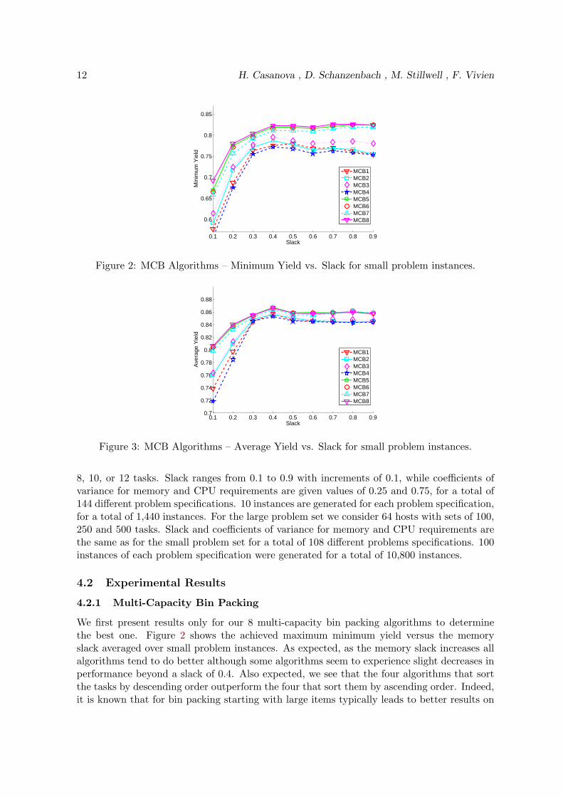
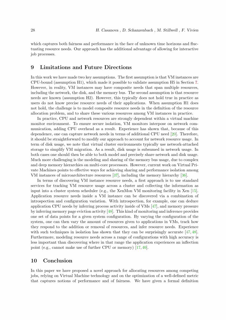
Figure 2: MCB Algorithms – Minimum Yield vs. Slack for small problem instances.
0.1 0.2 0.3 0.4 0.5 0.6 0.7 0.8 0.90.7
0.72
0.74
0.76
0.78
0.8
0.82
0.84
0.86
0.88
Slack
Ave
rage
Yie
ld
MCB1MCB2MCB3MCB4MCB5MCB6MCB7MCB8
Figure 3: MCB Algorithms – Average Yield vs. Slack for small problem instances.
8, 10, or 12 tasks. Slack ranges from 0.1 to 0.9 with increments of 0.1, while coefficients ofvariance for memory and CPU requirements are given values of 0.25 and 0.75, for a total of144 different problem specifications. 10 instances are generated for each problem specification,for a total of 1,440 instances. For the large problem set we consider 64 hosts with sets of 100,250 and 500 tasks. Slack and coefficients of variance for memory and CPU requirements arethe same as for the small problem set for a total of 108 different problems specifications. 100instances of each problem specification were generated for a total of 10,800 instances.
4.2 Experimental Results
4.2.1 Multi-Capacity Bin Packing
We first present results only for our 8 multi-capacity bin packing algorithms to determinethe best one. Figure 2 shows the achieved maximum minimum yield versus the memoryslack averaged over small problem instances. As expected, as the memory slack increases allalgorithms tend to do better although some algorithms seem to experience slight decreases inperformance beyond a slack of 0.4. Also expected, we see that the four algorithms that sortthe tasks by descending order outperform the four that sort them by ascending order. Indeed,it is known that for bin packing starting with large items typically leads to better results on
Resource Allocation using Virtual Clusters 13
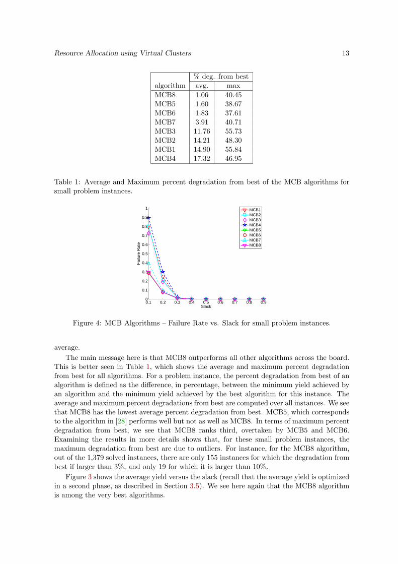
% deg. from bestalgorithm avg. maxMCB8 1.06 40.45MCB5 1.60 38.67MCB6 1.83 37.61MCB7 3.91 40.71MCB3 11.76 55.73MCB2 14.21 48.30MCB1 14.90 55.84MCB4 17.32 46.95
Table 1: Average and Maximum percent degradation from best of the MCB algorithms forsmall problem instances.
0.1 0.2 0.3 0.4 0.5 0.6 0.7 0.8 0.90
0.1
0.2
0.3
0.4
0.5
0.6
0.7
0.8
0.9
1
Slack
Fai
lure
Rat
e
MCB1MCB2MCB3MCB4MCB5MCB6MCB7MCB8
Figure 4: MCB Algorithms – Failure Rate vs. Slack for small problem instances.
average.The main message here is that MCB8 outperforms all other algorithms across the board.
This is better seen in Table 1, which shows the average and maximum percent degradationfrom best for all algorithms. For a problem instance, the percent degradation from best of analgorithm is defined as the difference, in percentage, between the minimum yield achieved byan algorithm and the minimum yield achieved by the best algorithm for this instance. Theaverage and maximum percent degradations from best are computed over all instances. We seethat MCB8 has the lowest average percent degradation from best. MCB5, which correspondsto the algorithm in [28] performs well but not as well as MCB8. In terms of maximum percentdegradation from best, we see that MCB8 ranks third, overtaken by MCB5 and MCB6.Examining the results in more details shows that, for these small problem instances, themaximum degradation from best are due to outliers. For instance, for the MCB8 algorithm,out of the 1,379 solved instances, there are only 155 instances for which the degradation frombest if larger than 3%, and only 19 for which it is larger than 10%.
Figure 3 shows the average yield versus the slack (recall that the average yield is optimizedin a second phase, as described in Section 3.5). We see here again that the MCB8 algorithmis among the very best algorithms.

14 H. Casanova , D. Schanzenbach , M. Stillwell , F. Vivien
6 7 8 9 10 11 120
0.5
1
1.5
2
2.5
3
3.5
4
4.5
5x 10
−4
Tasks
Run
Tim
e (s
ecs.
)
MCB1MCB2MCB3MCB4MCB5MCB6MCB7MCB8
Figure 5: MCB Algorithms – Run time vs. Number of Tasks for small problems instances.
0.1 0.2 0.3 0.4 0.5 0.6 0.7 0.8 0.90.3
0.35
0.4
0.45
0.5
0.55
Slack
Min
imum
Yie
ld
MCB1MCB2MCB3MCB4MCB5MCB6MCB7MCB8
Figure 6: MCB Algorithms – Minimum Yield vs. Slack for large problem instances.
Figure 4 shows the failure rates of the 8 algorithms versus the memory slack. As expectedfailure rates decrease as the memory slack increases, and as before we see that the fouralgorithms that sort tasks by descending order outperform the algorithms that sort tasks byascending order. Finally, Figure 5 shows the runtime of the algorithms versus the number oftasks. We use a 3.2GHz Intel Xeon processor. All algorithms have average run times under0.18 milliseconds, with MCB8 the fastest by a tiny margin.
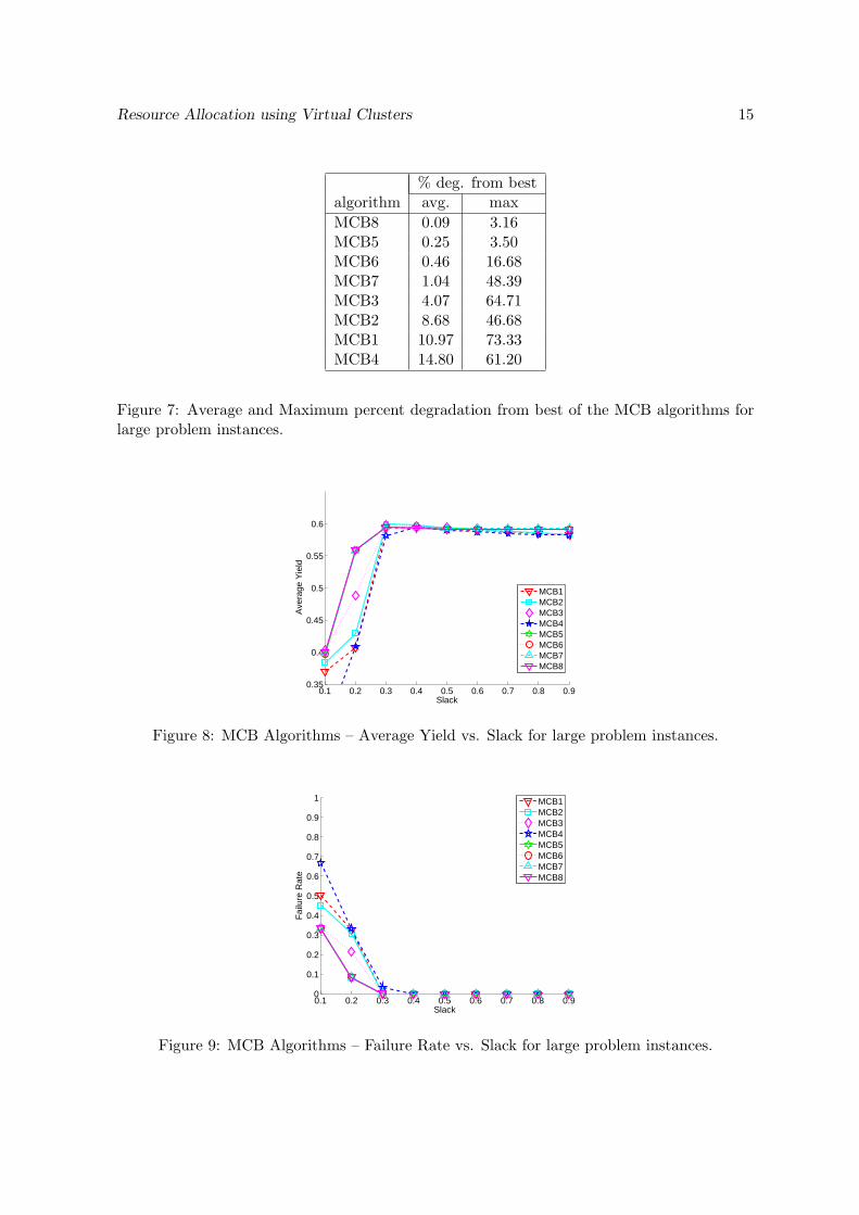
Figures 6, 8, 9, and 10 are similar to Figures 2, 3, 4, and 5, but show results for largeproblem instances. The message is the same here: MCB8 is the best algorithm, or closeron average to the best than the other algorithms. This is clearly seen in Table 7, whichis similar to Table 1, and shows the average and maximum percent degradation from bestfor all algorithms for large problem instances. According to both metrics MCB8 is the bestalgorithm, with MCB5 performing well but not as well as MCB8.
In terms of run times, Figure 10 shows run times under one-half second for 500 tasks forall of the MCB algorithms. MCB8 is again the fastest by a tiny margin.
Based on our results we conclude that MCB8 is the best option among the 8 multi-capacity bin packing options. In all that follows, to avoid graph clutter, we exclude the 7other algorithms from our overall results.
Resource Allocation using Virtual Clusters 15
% deg. from bestalgorithm avg. maxMCB8 0.09 3.16MCB5 0.25 3.50MCB6 0.46 16.68MCB7 1.04 48.39MCB3 4.07 64.71MCB2 8.68 46.68MCB1 10.97 73.33MCB4 14.80 61.20
Figure 7: Average and Maximum percent degradation from best of the MCB algorithms forlarge problem instances.
0.1 0.2 0.3 0.4 0.5 0.6 0.7 0.8 0.90.35
0.4
0.45
0.5
0.55
0.6
Slack
Ave
rage
Yie
ld
MCB1MCB2MCB3MCB4MCB5MCB6MCB7MCB8
Figure 8: MCB Algorithms – Average Yield vs. Slack for large problem instances.
0.1 0.2 0.3 0.4 0.5 0.6 0.7 0.8 0.90
0.1
0.2
0.3
0.4
0.5
0.6
0.7
0.8
0.9
1
Slack
Fai
lure
Rat
e
MCB1MCB2MCB3MCB4MCB5MCB6MCB7MCB8
Figure 9: MCB Algorithms – Failure Rate vs. Slack for large problem instances.

16 H. Casanova , D. Schanzenbach , M. Stillwell , F. Vivien
100 150 200 250 300 350 400 450 5000
0.1
0.2
0.3
0.4
0.5
0.6
0.7
0.8
0.9
1
Tasks
Run
Tim
e (s
ecs.
)
MCB1MCB2MCB3MCB4MCB5MCB6MCB7MCB8
Figure 10: MCB Algorithms – Run time vs. Number of Tasks for large problem instances.
0.1 0.2 0.3 0.4 0.5 0.6 0.7 0.8 0.9
0.6
0.65
0.7
0.75
0.8
0.85
Slack
Min
imum
Yie
ld
boundoptimalMCB8GRGBSGSGBRRNDRRNZ
Figure 11: Minimum Yield vs. Slack for small problem instances.
4.2.2 Small Problems
Figure 11 shows the achieved maximum minimum yield versus the memory slack in the systemfor our algorithms, the MILP solution, and for the solution of the rational LP, which is anupper bound on the achievable solution. The solution of the LP is only about 4% higher onaverage than that of the MILP, although it is significantly higher for very low slack values.The solution of the LP will be interesting for large problem instances, for which we cannotcompute an exact solution. On average, the exact MILP solution is about 2% better thanMCB8, and about 11% to 13% better than the greedy algorithms. All greedy algorithmsexhibit roughly the same performance. The RRND and RRNZ algorithms lead to resultsmarkedly poorer than the other algorithms, with expectedly the RRNZ algorithm slightlyoutperforming the RRND algorithm. Interestingly, once the slack reaches 0.2 the results ofboth the RRND and RRNZ algorithms begin to worsen.
Figure 12 is similar to Figure 11 but plots the average yield. The solution to the rationalLP, the MILP solution, the MCB8 solution, and the solutions produced by the greedy algo-rithms are all within a few percent of each other. As in Figure 11, when the slack is lowerthan 0.2 the relaxed solution is significantly better.
Figure 13 plots the failure rates of our algorithms. The RRND algorithm has the worst

Resource Allocation using Virtual Clusters 17
0.1 0.2 0.3 0.4 0.5 0.6 0.7 0.8 0.90.7
0.72
0.74
0.76
0.78
0.8
0.82
0.84
0.86
0.88
Slack
Ave
rage
Yie
ld
boundoptimalMCB8GRGBSGSGBRRNDRRNZ
Figure 12: Average Yield vs. Slack for small problem instances.
0.1 0.2 0.3 0.4 0.5 0.6 0.7 0.8 0.90
0.1
0.2
0.3
0.4
0.5
0.6
0.7
0.8
0.9
1
Slack
Fai
lure
Rat
e
optimalMCB8GRGBSGSGBRRNDRRNZ
Figure 13: Failure Rate vs. Slack for small problem instances.

18 H. Casanova , D. Schanzenbach , M. Stillwell , F. Vivien
6 7 8 9 10 11 120
0.5
1
1.5
2
2.5
3
3.5
4
4.5
5x 10
−4
Tasks
Run
Tim
e (s
ecs.
)
optimalMCB8GRGBSGSGBRRNDRRNZ
Figure 14: Run time vs. Number of Tasks for small problems instances.
failure rate, followed by GR and then RRNZ. There were a total of 60 instances out of the1,440 generated which were judged to be infeasible because the GLPK solver could not finda solution for them. We see that the MCB8, SG, and SGB algorithms have failure rates thatare not significantly larger than that of the exact MILP solution. Out of the 1,380 feasibleinstances, the GB and SGB never fail to find a solution, the MCB8 algorithm fails once, andthe SG algorithm fails 15 times.
Figure 14 shows the run times of the various algorithms on a 3.2GHz Intel Xeon processor.The computation time of the exact MILP solution is so much greater than that of the otheralgorithms that it cannot be seen on the graph. Computing the exact solution to the MILPtook an average of 28.7 seconds, however there were 9 problem instances with solutions thattook over 500 seconds to compute, and a single problem instance that required 11,549.29seconds (a little over 3 hours) to solve. For the small problem instances the average runtimes of all greedy algorithms and of the MCB8 algorithm are under 0.15 milliseconds, withthe simple GR and SG algorithms being the fastest. The RRND and RRNZ algorithms aresignificantly slower, with run times a little over 2 milliseconds on average; they also cannotbe seen on the graph.
4.2.3 Large Problems
Figures 15, 16, 17, and 18 are similar to Figures 11, 12, 13, and 14 respectively, but forlarge problem instances. In Figure 15 we can see that MCB8 algorithm achieves far betterresults than any other heuristic. Furthermore, MCB8 is extremely close to the upper boundas soon as the slack is 0.3 or larger and is only 8% away from this upper bound when theslack is 0.2. When the slack is 0.1, MCB8 is 37% away from the upper bound but we haveseen with the small problem instances that in this case the upper bound is significantly largerthan the actual optimal (see Figure 11).
The performance of the greedy algorithms has worsened relative to the rational LP so-lution, on average 20% lower for slack values larger than 0.2. The GR and GB algorithmsperform nearly identically, showing that backtracking does not help on the large probleminstances. The RRNZ algorithm is again a poor performer, with a profile that, unexpectedly,

Resource Allocation using Virtual Clusters 19
drops as slack increases. The RRND algorithm not only achieved the lowest values for min-imum yield, but also completely failed to solve any instances of the problem for slack valuesless than 0.4.
Figure 16 shows the achieved average yield values. The MCB8 algorithm again tracksthe optimal for slack values larger than 0.3. A surprising observation at first glance is thatthe greedy algorithms manage to achieve higher average yields than the optimal or MCBalgorithms. This is due to their lower achieved minimum yields. Indeed, with a lower minimumyield, average yield maximization is less constrained, making it possible to achieve higheraverage yield than when starting from and allocation optimal for the minimum yield. Thegreedy algorithms thus trade off fairness for higher average performance. The RRNZ algorithmstarts out doing well for average slack, even better than GR or GB when the slack is low, butdoes much worse as slack increases.
Figure 17 shows that for large problem instances the GB and SGB algorithms have nearlyas many failures as the GR and SG algorithms when slack is low. This suggests that thearbitrary bound of 500,000 placement attempts when backtracking, which was more thansufficient for the small problem set, has little affect on overall performance for the largeproblem set. It could thus be advisable to set the bound on the number of placement attemptsbased on the size of the problem set and time allowed for computation. The RRND algorithmis the only algorithm with a significant number of failures for slack values larger than 0.3. TheSG, SGB and MCB8 algorithms exhibit the lowest failure rates, about 40% lower than thatexperienced by the other greedy and RRNZ algorithms, and more than 14 times lower thanthe failure rate of the RRND algorithm. Keep in mind that, based on our experience withthe small problem set, some of the problem instances with small slacks may not be feasibleat all.
Figure 18 plots the average time needed to compute the solution to VCSched on a 3.2GHzIntel Xeon for all the algorithms versus the number of jobs. The RRND and RRNZ algorithmsrequire significant time, up to roughly 650 seconds on average for 500 tasks, and so cannotbe seen at the given scale. This is attributed to solving the relaxed MILP using GLPK. Notethat this time could be reduced significantly by using a faster solver (e.g., CPLEX [14]). TheGB and SGB algorithms require significantly more time when the number of tasks is small.This is because the failure rate decreases as the number of tasks increases. For a given set ofparameters, increasing the number of tasks decreases granularity. Since there is a relativelylarge number of unsolvable problems when the number of tasks is small, these algorithmsspend a lot of time backtracking and searching though the solution space fruitlessly, ultimatelystopping only when the bounded number of backtracking attempts is reached. The greedyalgorithms are faster than the MCB8 algorithm, returning solutions in 15 to 20 millisecondson average for 500 tasks as compared to nearly half a second for MCB8. Nevertheless, lessthan .5 seconds for 500 tasks is clearly acceptable in practice.
4.2.4 Discussion
Our main result is that the multi-capacity bin packing algorithm that sorts tasks in descendingorder by their largest resource requirement (MCB8) is the algorithm of choice. It outperformsor equals all other algorithm nearly across the board in terms of minimum yield, average yield,and failure rate, while exhibiting relatively low run times. The sorted greedy algorithms (SGor SGB) lead to reasonable results and could be used for very large numbers of tasks, for whichthe run time of MCB8 may become too high. The use of backtracking in the algorithms GB

20 H. Casanova , D. Schanzenbach , M. Stillwell , F. Vivien
0.1 0.2 0.3 0.4 0.5 0.6 0.7 0.8 0.90.3
0.35
0.4
0.45
0.5
0.55
Slack
Min
imum
Yie
ld
boundMCB8GRGBSGSGBRRNDRRNZ
Figure 15: Minimum Yield vs. Slack for large problem instances.
0.1 0.2 0.3 0.4 0.5 0.6 0.7 0.8 0.90.35
0.4
0.45
0.5
0.55
0.6
0.65
Slack
Ave
rage
Yie
ld
boundMCB8GRGBSGSGBRRNDRRNZ
Figure 16: Average Yield vs. Slack for large problem instances.
0.1 0.2 0.3 0.4 0.5 0.6 0.7 0.8 0.90
0.1
0.2
0.3
0.4
0.5
0.6
0.7
0.8
0.9
1
Slack
Fai
lure
Rat
e
MCB8GRGBSGSGBRRNDRRNZ
Figure 17: Failure Rate vs. Slack for large problem instances.

Resource Allocation using Virtual Clusters 21
100 150 200 250 300 350 400 450 5000
0.1
0.2
0.3
0.4
0.5
0.6
0.7
0.8
0.9
1
Tasks
Run
Tim
e (s
ecs.
)
MCB8GRGBSGSGBRRNDRRNZ
Figure 18: Run time vs. Number of Tasks for large problem instances.
and SGB led to performance improvements for small problem sets but not for large problemsets, suggesting that some sort of backtracking system with a problem-size- or run-time-dependent bound on the number of branches to explore could potentially be effective.
5 Parallel Jobs
5.1 Problem Formulation
In this section we explain how our approach and algorithms can be easily extended to handleparallel jobs that consist of multiple tasks (relaxing assumption H3). We have thus far onlyconcerned ourselves with independent jobs that are both indivisible and small enough to runon a single machine. However, in many cases users may want to split up jobs into multipletasks, either because they wish to use more CPU power in order to return results more quicklyor because they wish to process an amount of data that does not fit comfortably within thememory of a single machine.
One naıve way to extend our approach to parallel jobs would be to simply consider thetasks of a job independently. In this case individual tasks of the same job could then receivedifferent CPU allocations. However, in the vast majority of parallel jobs it is not useful tohave some tasks run faster than others as either the job makes progress at the rate of theslowest task or the job is deemed complete only when all tasks have completed. Therefore,we opt to add constraints to our linear program to enforce that the CPU allocations of taskswithin the same job must be identical. It would be straightforward to have more sophisticatedconstraints if specific knowledge about a particular job is available (e.g., task A should receivetwice as much CPU as task B).
Another important issue here is the possibility of gaming the system when optimizingthe average yield. When optimizing the minimum yield, a division of a job into multipletasks that leads to a higher minimum yield benefits all jobs. However, when considering theaverage yield optimization, which is done in our approach as a second round of optimization,a problem arises because the average yield metric favors small tasks, that is, tasks that havelow CPU requirements. Indeed, when given the choice to increase the CPU allocation of asmall task or of a larger task, for the same additional fraction of CPU, the absolute yieldincrease would be larger for the small task, and thus would lead to a higher average yield.
22 H. Casanova , D. Schanzenbach , M. Stillwell , F. Vivien
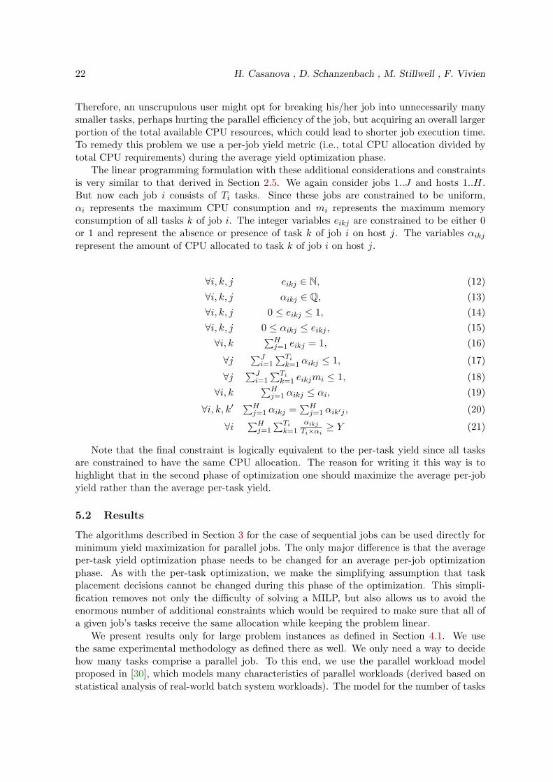
Therefore, an unscrupulous user might opt for breaking his/her job into unnecessarily manysmaller tasks, perhaps hurting the parallel efficiency of the job, but acquiring an overall largerportion of the total available CPU resources, which could lead to shorter job execution time.To remedy this problem we use a per-job yield metric (i.e., total CPU allocation divided bytotal CPU requirements) during the average yield optimization phase.
The linear programming formulation with these additional considerations and constraintsis very similar to that derived in Section 2.5. We again consider jobs 1..J and hosts 1..H.But now each job i consists of Ti tasks. Since these jobs are constrained to be uniform,αi represents the maximum CPU consumption and mi represents the maximum memoryconsumption of all tasks k of job i. The integer variables eikj are constrained to be either 0or 1 and represent the absence or presence of task k of job i on host j. The variables αikjrepresent the amount of CPU allocated to task k of job i on host j.
∀i, k, j eikj ∈ N, (12)∀i, k, j αikj ∈ Q, (13)∀i, k, j 0 ≤ eikj ≤ 1, (14)∀i, k, j 0 ≤ αikj ≤ eikj , (15)∀i, k
∑Hj=1 eikj = 1, (16)
∀j∑Ji=1
∑Tik=1 αikj ≤ 1, (17)
∀j∑Ji=1
∑Tik=1 eikjmi ≤ 1, (18)
∀i, k∑Hj=1 αikj ≤ αi, (19)
∀i, k, k′∑Hj=1 αikj =
∑Hj=1 αik′j , (20)
∀i∑Hj=1
∑Tik=1
αikj
Ti×αi≥ Y (21)
Note that the final constraint is logically equivalent to the per-task yield since all tasksare constrained to have the same CPU allocation. The reason for writing it this way is tohighlight that in the second phase of optimization one should maximize the average per-jobyield rather than the average per-task yield.
5.2 Results
The algorithms described in Section 3 for the case of sequential jobs can be used directly forminimum yield maximization for parallel jobs. The only major difference is that the averageper-task yield optimization phase needs to be changed for an average per-job optimizationphase. As with the per-task optimization, we make the simplifying assumption that taskplacement decisions cannot be changed during this phase of the optimization. This simpli-fication removes not only the difficulty of solving a MILP, but also allows us to avoid theenormous number of additional constraints which would be required to make sure that all ofa given job’s tasks receive the same allocation while keeping the problem linear.
We present results only for large problem instances as defined in Section 4.1. We usethe same experimental methodology as defined there as well. We only need a way to decidehow many tasks comprise a parallel job. To this end, we use the parallel workload modelproposed in [30], which models many characteristics of parallel workloads (derived based onstatistical analysis of real-world batch system workloads). The model for the number of tasks

Resource Allocation using Virtual Clusters 23
0.1 0.2 0.3 0.4 0.5 0.6 0.7 0.8 0.90.3
0.35
0.4
0.45
0.5
0.55
Slack
Min
imum
Yie
ld
boundMCB8SG
Figure 19: Minimum Yield vs. Slack for large problem instances for parallel jobs.
0.1 0.2 0.3 0.4 0.5 0.6 0.7 0.8 0.90.35
0.4
0.45
0.5
0.55
0.6
0.65
Slack
Ave
rage
Job
Yie
ld
boundMCB8SG
Figure 20: Average Yield vs. Slack for large problem instances for parallel jobs.
in a parallel job uses a two-stage log-uniform distribution biased towards powers of two. Weinstantiate this model using the same parameters as in [30], assuming that jobs can consistof between 1 and 64 tasks.
Figure 19 shows results for the SG and the MCB8 algorithms. We exclude all other greedyalgorithms as they were all shown to be outperformed by SG, all other MCB algorithmsbecause they were all shown to be outperformed by MCB8, as well as the RRND and RRNZalgorithms which were shown to perform poorly. The figure also shows the upper bound onoptimal obtained assuming that eij variables can take rational values. We see that MCB8outperforms the SGB algorithm significantly and is close to the upper bound on optimal forslacks larger than 0.3.
Figure 20 shows the average job yield. We see the same phenomenon as in Figure 16,namely that the greedy algorithm can achieve higher average yield because it starts from alower minimum yield, and thus has more options to push the average yield higher (therebyimproving average performance at the expense of fairness).
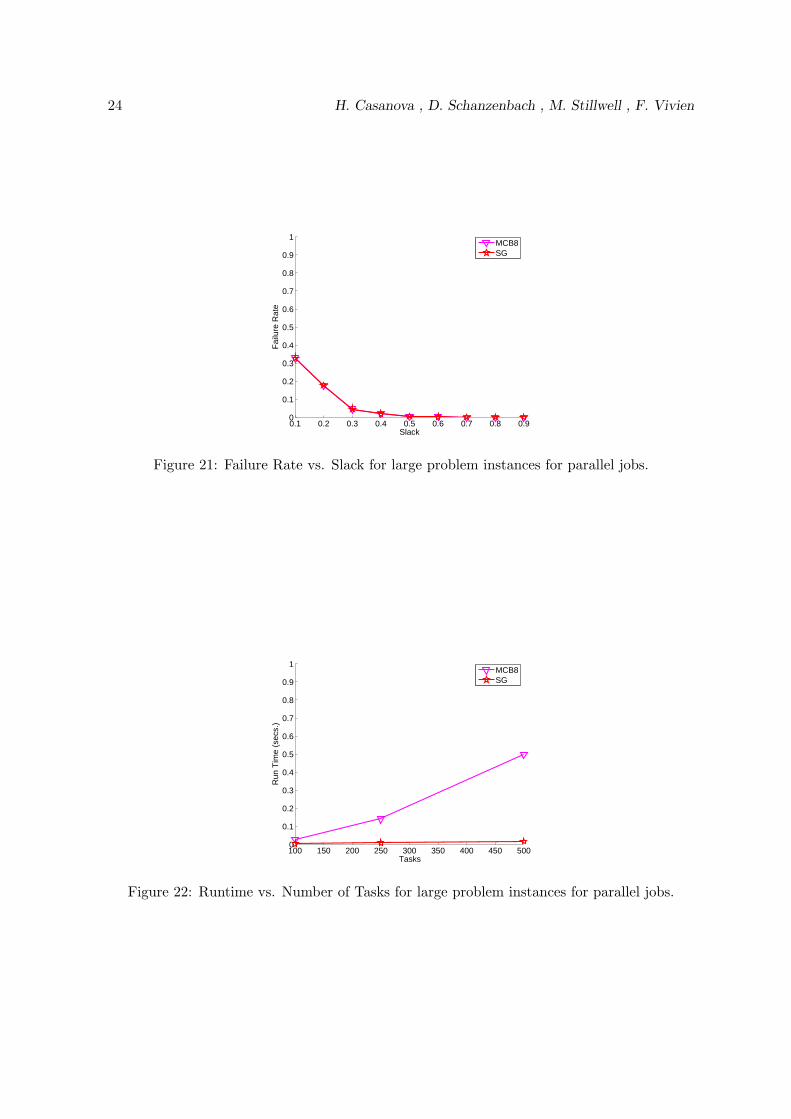
Figure 21 shows the failure rates of the MCB8 and SG algorithms, which are identical.Finally Figure 22 shows the run time of both algorithms. We see that the SG algorithm ismuch faster than the MCB8 algorithm (by roughly a factor 32 for 500 tasks). Nevertheless,MCB8 can still compute an allocation in under one half a second for 500 tasks.
24 H. Casanova , D. Schanzenbach , M. Stillwell , F. Vivien
0.1 0.2 0.3 0.4 0.5 0.6 0.7 0.8 0.90
0.1
0.2
0.3
0.4
0.5
0.6
0.7
0.8
0.9
1
Slack
Fai
lure
Rat
e
MCB8SG
Figure 21: Failure Rate vs. Slack for large problem instances for parallel jobs.
100 150 200 250 300 350 400 450 5000
0.1
0.2
0.3
0.4
0.5
0.6
0.7
0.8
0.9
1
Tasks
Run
Tim
e (s
ecs.
)
MCB8SG
Figure 22: Runtime vs. Number of Tasks for large problem instances for parallel jobs.
Resource Allocation using Virtual Clusters 25
Our conclusions are similar to the ones we made when examining results for sequentialjobs: in the case of parallel jobs the BCB8 algorithm is the algorithm of choice for optimizingminimum yield, while the SGB algorithm could be an alternate choice if the number of tasksis very large.
6 Dynamic Workloads
In this section we study resource allocation in the case when assumption H4 no longer holds,meaning that the workload is no longer static. We assume that job resource requirementscan change and that jobs can join and leave the system. When the workload changes, onemay wish to adapt the schedule to reach a new (nearly) optimal allocation of resources tothe jobs. This adaptation can entail two types of actions: (i) modifying the CPU fractionsallocated to some jobs; and (ii) migrating jobs to different physical hosts. In what follows weextend the linear program formulation derived in Section 2.5 to account for resource allocationadaptation. We then discuss how current technology can be used to implement adaptationwith virtual clusters.
6.1 Mixed-Integer Linear Program Formulation
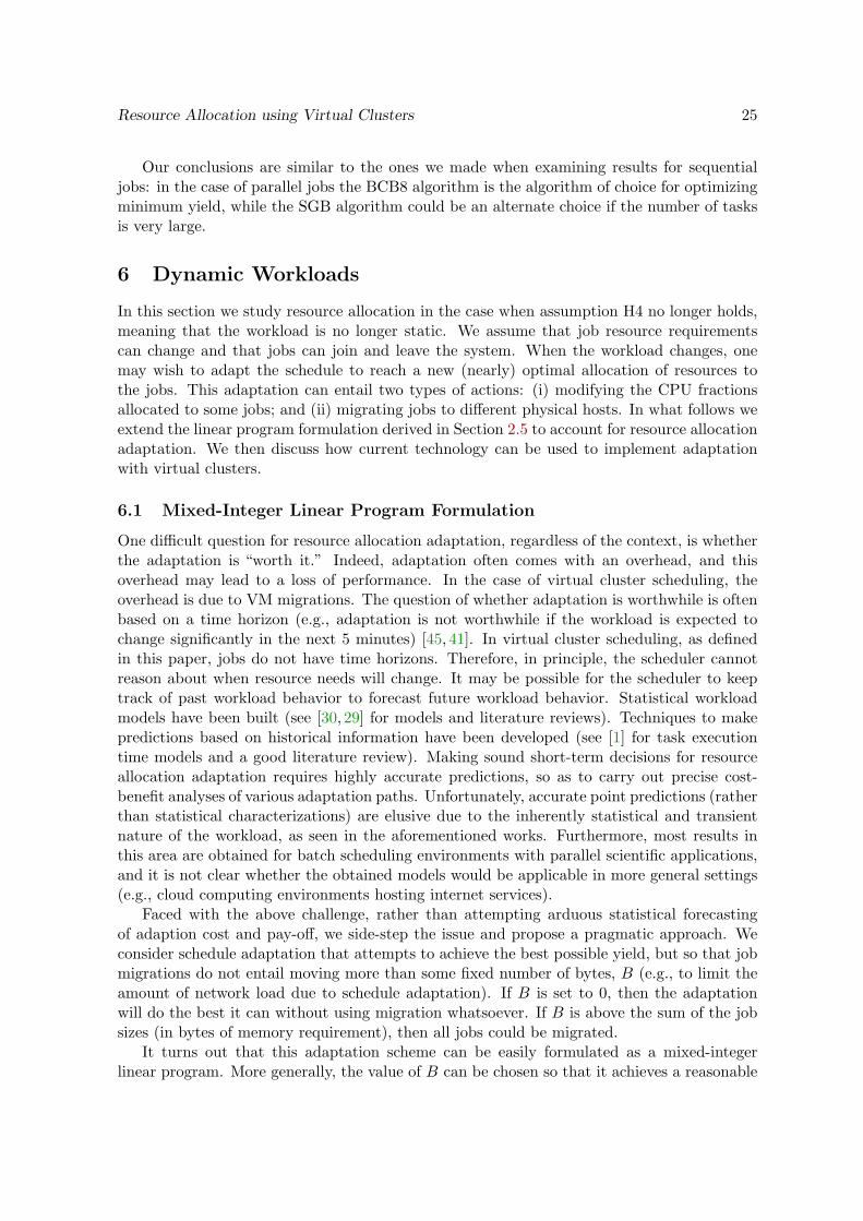
One difficult question for resource allocation adaptation, regardless of the context, is whetherthe adaptation is “worth it.” Indeed, adaptation often comes with an overhead, and thisoverhead may lead to a loss of performance. In the case of virtual cluster scheduling, theoverhead is due to VM migrations. The question of whether adaptation is worthwhile is oftenbased on a time horizon (e.g., adaptation is not worthwhile if the workload is expected tochange significantly in the next 5 minutes) [45, 41]. In virtual cluster scheduling, as definedin this paper, jobs do not have time horizons. Therefore, in principle, the scheduler cannotreason about when resource needs will change. It may be possible for the scheduler to keeptrack of past workload behavior to forecast future workload behavior. Statistical workloadmodels have been built (see [30, 29] for models and literature reviews). Techniques to makepredictions based on historical information have been developed (see [1] for task executiontime models and a good literature review). Making sound short-term decisions for resourceallocation adaptation requires highly accurate predictions, so as to carry out precise cost-benefit analyses of various adaptation paths. Unfortunately, accurate point predictions (ratherthan statistical characterizations) are elusive due to the inherently statistical and transientnature of the workload, as seen in the aforementioned works. Furthermore, most results inthis area are obtained for batch scheduling environments with parallel scientific applications,and it is not clear whether the obtained models would be applicable in more general settings(e.g., cloud computing environments hosting internet services).
Faced with the above challenge, rather than attempting arduous statistical forecastingof adaption cost and pay-off, we side-step the issue and propose a pragmatic approach. Weconsider schedule adaptation that attempts to achieve the best possible yield, but so that jobmigrations do not entail moving more than some fixed number of bytes, B (e.g., to limit theamount of network load due to schedule adaptation). If B is set to 0, then the adaptationwill do the best it can without using migration whatsoever. If B is above the sum of the jobsizes (in bytes of memory requirement), then all jobs could be migrated.
It turns out that this adaptation scheme can be easily formulated as a mixed-integerlinear program. More generally, the value of B can be chosen so that it achieves a reasonable

26 H. Casanova , D. Schanzenbach , M. Stillwell , F. Vivien
trade-off between overhead and workload dynamicity. Choosing the best value for B for aparticular system could however be difficult and may need to be adaptive as most workloadsare non-stationary. A good approach is likely to pick relatively smaller values of B for moredynamic workload. We leave a study of how to best tune parameter B for future work.
We use the same notations and definitions as in Section 2.5. In addition, we consider thatsome jobs are already assigned to a host: eij is equal to 1 if job i is already running on hostj, and 0 otherwise. For reasons that will be clear after we explain our constraints, we simplyset eij to 1 for all j if job i corresponds to a newly arrived job. Newly departed jobs need notbe taken into account. We can now write a new set of constraints as follows:
∀i, j eij ∈ N, (22)∀i, j αij ∈ Q, (23)∀i, j 0 ≤ eij ≤ 1, (24)∀i, j 0 ≤ αij ≤ eij , (25)∀i
∑Hj=1 eij = 1, (26)
∀j∑Ti=1 αij ≤ 1, (27)
∀j∑Ti=1 eijmi ≤ 1 (28)
∀i∑Hj=1 αij ≤ αi (29)
∀i∑Hj=1
αij
αi≥ Y (30)∑T
i=1
∑Hj=1(1− eij)eijmi ≤ B (31)
The objective, as in Section 2.5, is to maximize Y . The only new constraint is the lastone. This constraint simply states that if job i is assigned to a host that is different from thehost to which it was assigned previously, then it needs to be migrated. Therefore, mi bytesneed to be transferred. These bytes are summed over all jobs in the system to ensure that thetotal number of bytes communicated for migration purposes does not exceed B. Note thatthis is still a linear program as eij is not a variable but a constant. Since for newly arrivedjobs we set all eij values to 1, we can see that they do not contribute to the migration cost.Note that removing mi in the last constraint would simply mean that B is a bound on thetotal number of job migrations allowed during schedule adaptation.
We leave the development of heuristic algorithms for solving the above linear program forfuture work.
6.2 Technology Issues for Resource Allocation Adaptation
In the linear program in the previous section nowhere do we account for the time it takesto migrate a job. While a job is being migrated it is presumably non responsive, whichimpacts the yield. However, modern VM monitors support “live migration” of VM instances,which allows migrations with only milliseconds of unresponsiveness [13]. There could be aperformance degradation due to memory pages being migrated between two physical hosts.Resource allocation adaptation also requires quick modification of the CPU share allocatedto a VM instance (assumption H5). We validate this assumption in Section 7 and find that,indeed, CPU shares can be modified accurately in under a second.
Resource Allocation using Virtual Clusters 27
7 Evaluation of the Xen Hypervisor
Assumption H5 in Section 2.2 states that VM technology allows for precise, low-overhead,and quickly adaptable sharing of the computational capabilities of a host across CPU-boundVM instances. Although this seems like a natural expectation, we nevertheless validatethis assumption with state-of-the-art virtualization technology, namely, the Xen VM mon-itor [8]. While virtualization can happen inside the operating system (e.g, Virtual PC [34],VMWare [53]), Xen runs between the hardware and the operating system. It thus requireseither a modified operating system (“paravirtualization”) or hardware support for virtual-ization (“hardware virtualization” [21]). In this work we use Xen 3.1 on a dual-CPU 64-bitmachine with paravirtualization. All our VM instances use identical 64-bit Fedora images, areallocated 700MB of RAM, and run on the same physical CPU. The other CPU is used to runthe experiment controller. All our VM instances perform continuous CPU-bound computa-tions, that is, 100×100 double precision matrix multiplications using the LAPACK DGEMMroutine [5].
Our experiments consist in running from one to ten VM instances with specified “capvalues”, which Xen uses to control what fraction of the CPU is allocated to each VM. Wemeasure the effective compute rate of each VM instance (in number of matrix multiplicationsper seconds). We compare this rate to the expected rate, that is, the cap value times thecompute rate measured on the raw hardware. We can thus ascertain both the accuracy andthe overhead of the CPU-sharing in Xen. We also conduct experiments in which we change capvalues on-the-fly and measure the delay before the effective compute rates are in agreementwith the new cap values.
Due to space limitations we only provide highlights of our results and refer the readerto a technical report for full details [43]. We found that Xen imposes a minimal overhead(on average a 0.27% slowdown). We also found that the absolute error between the effectivecompute rate and the expected compute rate was at most 5.99% and on average 0.72%. Interms of responsiveness, we found that the effective compute rate of a VM becomes congruentwith a cap value less than one second after that cap value was changed. We conclude that,in the case of CPU-bound VM instances, CPU-sharing in Xen is sufficiently accurate andresponsive to enable fractional and dynamic resource allocations as defined in this paper.
8 Related Work
The use of virtual machine technology to improve parallel job reliability, cluster utilization,and power efficiency is a hot topic for research and development, with groups at severaluniversities and in industry actively developing resource management systems [32,3,2,19,42].This paper builds on top of such research, using the resource manager intelligently to optimizea user-centric metric that attempts to capture common ideas about fairness among the usersof high-performance systems.
Our work bears some similarities with gang scheduling. However, traditional gang schedul-ing approaches suffer from problems due to memory pressure and the communication expenseof coordinating context switches across multiple hosts [38, 9]. By explicitly considering taskmemory requirements when making scheduling decisions and using virtual machine technologyto multiplex the CPU resources of individual hosts our approach avoids these problems.
Above all, our approach is novel in that we define and optimize for a user-centric metric
28 H. Casanova , D. Schanzenbach , M. Stillwell , F. Vivien
which captures both fairness and performance in the face of unknown time horizons and fluc-tuating resource needs. Our approach has the additional advantage of allowing for interactivejob processes.
9 Limitations and Future Directions
In this work we have made two key assumptions. The first assumption is that VM instances areCPU-bound (assumption H1), which made it possible to validate assumption H5 in Section 7.However, in reality, VM instances may have composite needs that span multiple resources,including the network, the disk, and the memory bus. The second assumption is that resourceneeds are known (assumption H2). However, this typically does not hold true in practice asusers do not know precise resource needs of their applications. When assumption H1 doesnot hold, the challenge is to model composite resource needs in the definition of the resourceallocation problem, and to share these various resources among VM instances in practice.
In practice, CPU and network resources are strongly dependent within a virtual machinemonitor environment. To ensure secure isolation, VM monitors interpose on network com-munication, adding CPU overhead as a result. Experience has shown that, because of thisdependence, one can capture network needs in terms of additional CPU need [20]. Therefore,it should be straightforward to modify our approach to account for network resource usage. Interm of disk usage, we note that virtual cluster environments typically use network-attachedstorage to simplify VM migration. As a result, disk usage is subsumed in network usage. Inboth cases one should then be able to both model and precisely share network and disk usage.Much more challenging is the modeling and sharing of the memory bus usage, due to complexand deep memory hierarchies on multi-core processors. However, current work on Virtual Pri-vate Machines points to effective ways for achieving sharing and performance isolation amongVM instances of microarchitecture resources [37], including the memory hierarchy [36].
In terms of discovering VM instance resource needs, a first approach is to use standardservices for tracking VM resource usage across a cluster and collecting the information asinput into a cluster system scheduler (e.g., the XenMon VM monitoring facility in Xen [15].Application resource needs inside a VM instance can be discovered via a combination ofintrospection and configuration variation. With introspection, for example, one can deduceapplication CPU needs by inferring process activity inside of VMs [47], and memory pressureby inferring memory page eviction activity [48]. This kind of monitoring and inference providesone set of data points for a given system configuration. By varying the configuration of thesystem, one can then vary the amount of resources given to applications in VMs, track howthey respond to the addition or removal of resources, and infer resource needs. Experiencewith such techniques in isolation has shown that they can be surprisingly accurate [47, 48].Furthermore, modeling resource needs across a range of configurations with high accuracy isless important than discovering where in that range the application experiences an inflectionpoint (e.g., cannot make use of further CPU or memory) [17,40].
10 Conclusion
In this paper we have proposed a novel approach for allocating resources among competingjobs, relying on Virtual Machine technology and on the optimization of a well-defined metricthat captures notions of performance and of fairness. We have given a formal definition

Resource Allocation using Virtual Clusters 29
of a base problem, have proposed several algorithms to solve it, and have evaluated thesealgorithms in simulation. We have identified a promising algorithm that runs quickly, is onpar with or better than its competitors, and is close to optimal. We have then discussedseveral extensions to our approach to solve more general problems, namely when jobs areparallel, when the workload is dynamic, when job resource needs are composite, and whenjob resource needs are unknown.
Future directions include the development of algorithms to solve the resource allocationadaptation problem, and of strategies for estimating job resource needs accurately. Ourultimate goal is to develop a new resource allocator as part of the Usher system [32], so thatour algorithms and techniques can be used as part of a practical system and evaluated inpractical settings.
References
[1] Backfilling Using System-Generated Predictions Rather than User Runtime Estimates.IEEE Transactions on Parallel and Distributed Systems, 18(6):789–803, 2007.
[2] Citric xenserver enterprise edition. http://www.xensource.com/products/Pages/XenEnterprise.aspx, 2008.
[3] Virtualcenter. http://www.vmware.com/products/vi/vc, 2008.
[4] Amazon Elastic Compute Cloud. http://aws.amazon.com/ec2.
[5] E. Anderson, Z. Bai, C. Bischof, S. Blackford, J. Demmel, J. Dongarra, J. Du Croz,A. Greenbaum, S. Hammarling, A. McKenney, and D. Sorensen. LAPACK Users’ GuideThird Edition. Society for Industrial and Applied Mathematics, 1999.
[6] K. Baker. Introduction to Sequencing and Scheduling. Wiley, 1974.
[7] N. Bansal and M. Harchol-Balter. Analysis of SRPT Scheduling: Investigating Un-fairness. In Proceedings of ACM SIGMETRICS 2001 Conference on Measurement andModeling of Computer Systems, pages 279–290, June 2001.
[8] P. Barham, B. Dragovic, K. Fraser, S. Hand, T. Harris, A. Ho, R. Neugebauer, I. Pratt,and A. Warfield. Xen and the Art of Virtualization. In Proceedings of the ACM Sympo-sium on Operating Systems Principles, pages 164–177, October 2003.
[9] A. Batat and D. Feitelson. Gang scheduling with memory considerations. In Proceedingsof the 14th International Parallel and Distributed Processing Symposium, pages 109–114,2000.
[10] M. Bender, S. Chakrabarti, and S. Muthukrishnan. Flow and Stretch Metrics for Schedul-ing Continuous Job Streams. In Proceedings of the 9th Annual ACM-SIAM SymposiumOn Discrete Algorithms (SODA’98), pages 270–279, 1998.
[11] M. Bender, S. Muthukrishnan, and R. Rajamaran. Approximation Algorithms for Aver-age Stretch Scheduling. Journal of Scheduling, 7(3):195–222, 2004.
[12] J. Buisson, F. Andre, and J.-L. Pazat. A Framework for Dynamic Adaptation of ParallelComponents. In Proceedings of the International Conference ParCo, pages 65–72, 2005.
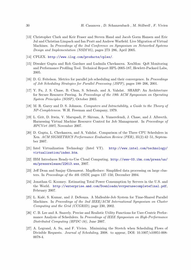
30 H. Casanova , D. Schanzenbach , M. Stillwell , F. Vivien
[13] Christopher Clark and Keir Fraser and Steven Hand and Jacob Gorm Hansen and EricJul and Christian Limpach and Ian Pratt and Andrew Warfield. Live Migration of VirtualMachines. In Proceedings of the 2nd Conference on Symposium on Networked SystemsDesign and Implementation (NSDI’05), pages 273–286, April 2005.
[14] CPLEX. http://www.ilog.com/products/cplex/.
[15] Diwaker Gupta and Rob Gardner and Ludmila Cherkasova. XenMon: QoS Monitoringand Performance Profiling Tool. Technical Report HPL-2005-187, Hewlett-Packard Labs,2005.
[16] D. G. Feitelson. Metrics for parallel job scheduling and their convergence. In Proceedingsof Job Scheduling Strategies for Parallel Processing (JSPP), pages 188–206, 2001.
[17] Y. Fu, J. S. Chase, B. Chun, S. Schwab, and A. Vahdat. SHARP: An Architecturefor Secure Resource Peering. In Proceedings of the 19th ACM Symposium on OperatingSystem Principles (SOSP), October 2003.
[18] M. R. Garey and D. S. Johnson. Computers and Intractability, a Guide to the Theory ofNP-Completeness. W.H. Freeman and Company, 1979.
[19] L. Grit, D. Itwin, V. Marupadi, P. Shivam, A. Yumerefendi, J. Chase, and J. Albrecth.Harnessing Virtual Machine Resource Control for Job Management. In Proceedings ofHPCVirt 2007, November 2007.
[20] D. Gupta, L. Cherkasova, and A. Vahdat. Comparison of the Three CPU Schedulers inXen. ACM SIGMETRICS Performance Evaluation Review (PER), 35(2):42–51, Septem-ber 2007.
[21] Intel Virtualization Technology (Intel VT). http://www.intel.com/technology/virtualization/index.htm.
[22] IBM Introduces Ready-to-Use Cloud Computing. http://www-03.ibm.com/press/us/en/pressrelease/22613.wss, 2007.
[23] Jeff Dean and Sanjay Ghemawat. MapReduce: Simplified data processing on large clus-ters. In Proceedings of the 6th OSDI, pages 137–150, December 2004.
[24] Jonathan G. Koomey. Estimating Total Power Consumption by Servers in the U.S. andthe World. http://enterprise.amd.com/Downloads/svrpwrusecompletefinal.pdf,February 2007.
[25] L. Kale, S. Kumar, and J. DeSouza. A Malleable-Job System for Time-Shared ParallelMachines. In Proceedings of the 2nd IEEE/ACM International Symposium on ClusterComputing and the Grid (CCGRID), page 230, 2002.
[26] C. B. Lee and A. Snavely. Precise and Realistic Utility Functions for User-Centric Perfor-mance Analysis of Schedulers. In Proceedings of IEEE Symposium on High-PerformanceDistributed Computing (HPDC-16), June 2007.
[27] A. Legrand, A. Su, and F. Vivien. Minimizing the Stretch when Scheduling Flows ofDivisible Requests. Journal of Scheduling, 2008. to appear, DOI: 10.1007/s10951-008-0078-4.

Resource Allocation using Virtual Clusters 31
[28] W. Leinberger, G. Karypis, and V. Kumar. Multi-capacity bin packing algorithms withapplications to job scheduling under multiple constraints. In Proceedings of the Interna-tional Conference on Parallel Processing, pages 404–412, 1999.
[29] H. Li. Workload Dynamics on Clusters and Grids. Journal of Supercomputing, 2008.on-line publication.
[30] U. Lublin and D. Feitelson. The Workload on Parallel Supercomputers: Modeling theCharacteristics of Rigid Jobs. Journal of Parallel and Distributed Computing, 63(11),2003.
[31] L. Marchal, Y. Yang, H. Casanova, and Y. Robert. Steady-state scheduling of multipledivisible load applications on wide-area distributed computing platforms. 20(3):365–381,2006.
[32] M. McNett, D. Gupta, A. Vahdat, and G. M. Voelker. Usher: An extensible frameworkfor managing clusters of virtual machines. In Proceedings of Lisa 2007, 2007.
[33] Michael Isard and Mihai Budiu and Yuan Yu and Andrew Birrell and Dennis Fetterly.Dryad: Distributed Data-Parallel Programs from Sequential Building Blocks. In Pro-ceedings of the European Conference on Computer Systems (EuroSys), March 2007.
[34] Microsoft Virtual PC. http://www.microsoft.com/windows/products/winfamily/virtualpc/default.mspx.
[35] S. Muthukrishnan, R. Rajaraman, A. Shaheen, and J. Gehrke. Online Scheduling toMinimize Average Stretch. In Proceedings of the IEEE Symposium on Foundations ofComputer Science, pages 433–442, 1999.
[36] K. Nesbit, J. Laudon, and J. Smith. Virtual Private Caches. In Proceedings of the 34thAnnual International Symposium on Computer Architecture (ISCA), June 2007.
[37] K. Nesbit, M. Moreto, F. Cazorla, A. Ramirez, and M. Valero. Multicore ResourceManagement. IEEE Micro, May-June 2008.
[38] J. Ousterhout. Scheduling Techniques for Concurrent Systems. In Proceedings of the 3rdInternational Conferance on Distributed Computing Systems, pages 22–30, 1982.
[39] A. H. Project. Hadoop. http://hadoop.apache.org/.
[40] R. H. Patterson and G. A. Gibson and E. Ginting and D. Stodolsky and J. Zelenka.Informed Prefetching and Caching. In Proceedings of the 15th Symposium of OperatingSystems Principles, October 1995.
[41] R. L. Ribler, H. Simitci, and D. A. Reed. The Autopilot Performance-Directed AdaptiveControl System. Future Generation Computer Systems, 18(1), 2001.
[42] P. Ruth, R. Junghwan, D. Xu, R. Kennell, and S. Goasguen. Autonomic Live Adaptationof Virtual Computational Environments in a Multi-Domain Infrastructure. In Proceedingsof the IEEE International Conference on Autonomic Computing, June 2006.

32 H. Casanova , D. Schanzenbach , M. Stillwell , F. Vivien
[43] D. Schanzenbach and H. Casanova. Accuracy and Responsiveness of CPU Sharing UsingXen’s Cap Values. Technical Report ICS2008-05-01, Computer and Information SciencesDept., University of Hawai‘i at Manoa, May 2008. available at http://www.ics.hawaii.edu/research/tech-reports/ICS2008-05-01.pdf/view.
[44] U. Schwiegelshohn and R. Yahyapour. Fairness in parallel job scheduling. Journal ofScheduling, 3(5):297–320, 2000.
[45] O. Sievert and H. Casanova. A Simple MPI Process Swapping Architecture for Itera-tive Applications. International Journal of High Performance Computing Applications,18(3):341–352, 2004.
[46] A. Sodan and X. Huang. Adaptive Time/Space Sharing with SCOJO. InternationalJournal of High Performance Computing and Networking, 4(5/6):256–269, 2006.
[47] Stephen T. Jones and Andrea C. Arpaci-Dusseau and Remzi H. Arpaci-Dusseau. Ant-farm: Tracking Processes in a Virtual Machine Environment. In Proceedings of theUSENIX Annual Technical Conference (USENIX ’06), June 2006.
[48] Stephen T. Jones and Andrea C. Arpaci-Dusseau and Remzi H. Arpaci-Dusseau. Geiger:Monitoring the Buffer Cache in a Virtual Machine Environment. In Proceedings of Ar-chitectural Support for Programming Languages and Operating Systems (ASPLOS XII),October 2006.
[49] Top500 supercomputer sites. http://www.top500.org, 2008.
[50] U.S. Environmental Protection Agency. Report to Congress on Server and Data Cen-ter Energy Efficiency. http://www.energystar.gov/ia/partners/prod_development/downloads/EPA_Datacenter_Report_Congress_Final1.pdf, August 2007.
[51] G. Utrera, J. Corbala, and J. Labarta. Implementing Malleability on MPI Jobs. InProceedings of 13th International Conference on Parallel Archtecture and CompilationTechniques (PACT), pages 215–224, 2004.
[52] S. Vadhiyar and J. Dongarra. SRS: A Framework for Developing Malleable and Migrat-able Parallel Applications for Distributed Systems. Parallel Processing Letters, 13(2):291–312, 2003.
[53] VMware. http://www.vmware.com/.