Embed Size (px)
Citation preview

DEPARTMENT OF INFORMATION ENGINEERING AND COMPUTER SCIENCE
ICT International Doctoral School
Resource Abstraction and Virtualization
Solutions for Wireless Networks
by
Anteneh Atumo Gebremariam
A dissertation submitted in partial fulfillment of the
requirements for the degree of
Doctor of Philosophy
AdvisorProf. Fabrizio Granelli
Universita degli Studi di Trento
Co-AdvisorDr. Leonardo Goratti
CREATE-NET Research Center
March 2017


Abstract
To cope up with the booming of data traffic and to accommodate new and emerging
technologies such as machine-type communications, Internet-of-Things, the 5th Genera-
tion (5G) of mobile networks require multiple complex operations (i.e., allocating non-
overlapping radio resources, monitoring interference, etc.). Software-defined networking
(SDN) and network function virtualization (NFV) are the two emerging technologies that
promise to provide programmability and flexibility in terms of managing, configuring and
optimizing wireless networks such that a better performance is achieved. In this disser-
tation, we particularly focus on inter-cell-interference (ICI) mitigation techniques and
efficient radio resource utilization schemes through the adoption of these two technologies
in wireless environment.
We exploit the SDN approach in order to expose the lower layers (i.e., physical and
medium access control) parameters of the wireless protocol stack to a centralized con-
trol module such that it is possible to dynamically configure the network in a logically
centralized manner, through specifically designed network functions (algorithms). In the
first part of this work, we proposed two ICI mitigation solutions, one via an Interference
Graph (IG) abstraction technique to control ICI in macro base stations and the second
one is through dynamic strict fractional frequency reuse technique to overcome the limita-
tions of ICI in dense small cell base station deployments where ICI arises from frequency
reuse one in multi-tier networks. Then based on the fractional frequency reuse (FFR)
technique, we propose a spatial scheduling schemes that aim to schedule users in the spa-
tial domain through layered schedulers operating in different time scales, short and long.
The cell coverage area is dynamically divided into multiple scheduling areas based on the
antenna beamwidth and steerable signal-to-interference-plus-noise-ratio (SINR) threshold
values. Simulation results show our proposed approaches outperform the legacy static FFR
schemes in terms of spectral efficiency, aggregate throughput and packet blocking proba-
bility. Moreover, we provided the detailed analysis of the computational complexity of our
proposed algorithms in comparison to the once existing in the literature.
The 5G networks will be built around people and things targeted to meet the require-
ments different groups of uses cases (i.e., massive broadband, massive machine-type com-
munication and critical machine-type communication). In order to support these services
it is very costly and impractical to make a separate dedicated network corresponding to
each of the services. The most attractive solution in terms of reducing cost at the same
time improving backward compatibility is through the implementation of service-dedicated

virtual networks, network slicing. Thus we proposed a dynamic spectrum-level slicing
algorithm to share radio resources across different virtual networks. Through virtualiza-
tion, the physical radio resources of the heterogeneous mobile networks are first abstracted
into a centralized pool of virtual radio resources. Then we investigated the performance
gains of our proposed algorithm though dynamically sharing the abstracted radio resources
across multiple virtual networks. Simulation results show that for representative user
arrival statistics, dynamic allocation of radio resources significantly lowers the percent-
age of dropped packets. Moreover, this work is the preliminary step towards enabling an
end-to-end network slicing for 5G mobile networking, which is the base for implement-
ing service differentiated virtual networks over a single physical infrastructure. Finally,
we presented a test-bed implementation of dynamic spectrum-level slicing algorithm us-
ing an open-source software/hardware platform called OpenAirInterface that emulates the
long-term evolution (LTE) protocol stack.
Keywords
[5G Networks, Long Term Evolution, Software-defined Networking, Network Function
Virtualization, Abstraction, Inter-Cell-Interference, Network Slicing, End-to-End Slicing,
OpenAirInterface]
4

Acknowledgement
Foremost, I would like express my sincere and heartfelt gratitude to Prof. Fabrizio
Granelli, for his excellent guidance and unlimited support throughout my PhD program. I
am sure it would have not been possible without his help. I am truly indebted and thankful
to Prof. Andrea Goldsmith, Dr. Leonardo Goratti, Dr. Domenico Siracusa, Dr. Roberto
Riggio and Dr. Tinku Rasheed without their active supervision, follow-up, support and
guidance this thesis work would not be accomplished. Specially, I owe earnest thankfulness
to Dr. Leonardo Goratti for being understanding, kind, patient, co-operative and helpful
in every aspect during the PhD. He played a critical role for successful completion of the
task. I also owe my deepest gratitude to Prof. Andrea Goldsmith, for making it possible
to visit her lab, providing unlimited help and transferring research skills that I will use
in my future career. I would like also to thank colleagues and friends in wireless systems
lab (WSL), Stanford univesity, for the collaboration work and amazing experience that I
had during my stay in Stanford. I am thankful for Julia Gillespie for all the support she
gave me while I was both in Trento and Standford. I also like to thank my colleagues at
university of Trento, the ICT doctoral office, Saud Althunibat, Raul Palacios, Qi Wang
and Muhammad Usman, for assistance, support and for the collaboration work. Besides,
I want to thank my friends and the special one for the beautiful memorable times and
giving a huge moral support in every step. Lastly but not least, I would like to thank my
beloved family, for their endless love, support and encouragement. Above all, I thank God
for fulfilling my dreams.


Contents
I Introduction, Outline and Literature Review 1
1 Introduction 3
1.1 Motivation . . . . . . . . . . . . . . . . . . . . . . . . . . . . . . . . . . . . 3
1.1.1 The Problem . . . . . . . . . . . . . . . . . . . . . . . . . . . . . . 5
1.2 Contributions of the Disertation . . . . . . . . . . . . . . . . . . . . . . . . 6
1.2.1 Innovative Aspects . . . . . . . . . . . . . . . . . . . . . . . . . . . 7
2 Outline and Scientific Product 9
2.1 Desertation Outline . . . . . . . . . . . . . . . . . . . . . . . . . . . . . . . 9
2.2 Scientific Product . . . . . . . . . . . . . . . . . . . . . . . . . . . . . . . . 10
3 Literature Review 13
3.1 SDN as applied to Wireless Networks . . . . . . . . . . . . . . . . . . . . . 13
3.2 ICI Mitigation . . . . . . . . . . . . . . . . . . . . . . . . . . . . . . . . . . 14
3.2.1 Interference Avoidance . . . . . . . . . . . . . . . . . . . . . . . . . 16
3.3 Wireless Network Virtualization . . . . . . . . . . . . . . . . . . . . . . . . 21
3.3.1 Components of Wireless Network Virtualization . . . . . . . . . . . 22
3.3.2 Main Enablers of Wireless Network Virtualization . . . . . . . . . . 25
3.3.3 Main Challenges of Wireless Network Virtualization . . . . . . . . . 29
3.4 Concluding Remarks . . . . . . . . . . . . . . . . . . . . . . . . . . . . . . 29
II Interference Mitigation Techniques 31
4 ICI Mitigation via Interference Graph 33
4.1 Introduction . . . . . . . . . . . . . . . . . . . . . . . . . . . . . . . . . . . 33
4.1.1 Related Work . . . . . . . . . . . . . . . . . . . . . . . . . . . . . . 34
4.2 System Model . . . . . . . . . . . . . . . . . . . . . . . . . . . . . . . . . . 35
i

4.2.1 SDN for cellular networks . . . . . . . . . . . . . . . . . . . . . . . 36
4.3 Problem Formulation . . . . . . . . . . . . . . . . . . . . . . . . . . . . . . 38
4.4 Interference Modeling . . . . . . . . . . . . . . . . . . . . . . . . . . . . . . 39
4.4.1 Interference Graph . . . . . . . . . . . . . . . . . . . . . . . . . . . 40
4.4.2 Conflict Graph Construction . . . . . . . . . . . . . . . . . . . . . . 40
4.5 Resource Allocation and Optimization . . . . . . . . . . . . . . . . . . . . 41
4.6 Summary . . . . . . . . . . . . . . . . . . . . . . . . . . . . . . . . . . . . 43
5 ICI Mitigation via FFR 45
5.1 Introduction . . . . . . . . . . . . . . . . . . . . . . . . . . . . . . . . . . . 45
5.1.1 Related Work . . . . . . . . . . . . . . . . . . . . . . . . . . . . . . 47
5.2 Main Contributions . . . . . . . . . . . . . . . . . . . . . . . . . . . . . . . 48
5.3 System Model . . . . . . . . . . . . . . . . . . . . . . . . . . . . . . . . . . 49
5.4 Algorithm Description . . . . . . . . . . . . . . . . . . . . . . . . . . . . . 51
5.5 System Analysis . . . . . . . . . . . . . . . . . . . . . . . . . . . . . . . . . 52
5.5.1 Probability of Coverage . . . . . . . . . . . . . . . . . . . . . . . . 52
5.5.2 Frequency Reuse One (FR1) . . . . . . . . . . . . . . . . . . . . . . 55
5.5.3 Centralized FFR (C-FFR) Approach . . . . . . . . . . . . . . . . . 56
5.5.4 Decentralized FFR (D-FFR) Approach . . . . . . . . . . . . . . . . 60
5.5.5 Computational Complexity Comparison . . . . . . . . . . . . . . . 61
5.6 Results . . . . . . . . . . . . . . . . . . . . . . . . . . . . . . . . . . . . . . 62
5.6.1 Performance Metrices . . . . . . . . . . . . . . . . . . . . . . . . . . 63
5.6.2 Numerical Results . . . . . . . . . . . . . . . . . . . . . . . . . . . 64
5.7 Summary . . . . . . . . . . . . . . . . . . . . . . . . . . . . . . . . . . . . 70
III Resource Slicing in Wireless Networks 73
6 Spectrum-level Slicing 75
6.1 Introduction . . . . . . . . . . . . . . . . . . . . . . . . . . . . . . . . . . . 75
6.1.1 Prior Work . . . . . . . . . . . . . . . . . . . . . . . . . . . . . . . 77
6.2 System Model . . . . . . . . . . . . . . . . . . . . . . . . . . . . . . . . . . 78
6.3 System Analysis . . . . . . . . . . . . . . . . . . . . . . . . . . . . . . . . . 80
6.3.1 Dynamic spectrum-level slicer . . . . . . . . . . . . . . . . . . . . . 80
6.3.2 User Traffic Model . . . . . . . . . . . . . . . . . . . . . . . . . . . 82
6.3.3 Key Performance Indicators . . . . . . . . . . . . . . . . . . . . . . 84
6.4 Numerical Results . . . . . . . . . . . . . . . . . . . . . . . . . . . . . . . . 85
ii

6.5 Summary . . . . . . . . . . . . . . . . . . . . . . . . . . . . . . . . . . . . 88
7 E2E Network Slicing 89
7.1 Introduction . . . . . . . . . . . . . . . . . . . . . . . . . . . . . . . . . . . 89
7.1.1 E2E Network Slicing . . . . . . . . . . . . . . . . . . . . . . . . . . 90
7.2 Evolved Packet Core Slicing . . . . . . . . . . . . . . . . . . . . . . . . . . 91
7.3 Radio Access Network Slicing . . . . . . . . . . . . . . . . . . . . . . . . . 94
7.3.1 OpenAirInterface based RAN Slicing . . . . . . . . . . . . . . . . . 95
7.3.2 OAI based Experimentation Results . . . . . . . . . . . . . . . . . . 96
7.4 Summary . . . . . . . . . . . . . . . . . . . . . . . . . . . . . . . . . . . . 99
IV Future Work and Conclusions 101
8 Future Work 103
9 Conclusions 105
Bibliography 107
iii


List of Tables
5.1 System parameter setting . . . . . . . . . . . . . . . . . . . . . . . . . . . 65
6.1 System parameter settings . . . . . . . . . . . . . . . . . . . . . . . . . . . . . 86
6.2 UE concentration in each VN . . . . . . . . . . . . . . . . . . . . . . . . . . . . 86
7.1 5G use case examples and their QoS requirements [72] . . . . . . . . . . . . . . . . 90
v


List of Figures
1.1 Control-plane and data-plane decoupling in SDN [5] . . . . . . . . . . . . . . . . . 4
3.1 The Communication of an OpenFlow enabled switch with a controller over a secure
channel using the OpenFlow protocol [16] . . . . . . . . . . . . . . . . . . . . . . 14
3.2 Co-tier ICI in homogeneous networks . . . . . . . . . . . . . . . . . . . . . . . . 15
3.3 Cross-tier ICI in HetNets . . . . . . . . . . . . . . . . . . . . . . . . . . . . . . 15
3.4 Inter-cell interference in an OFDMA based systems [24] . . . . . . . . . . . . . . . 16
3.5 PFR scheme: power allocation and frequency reuse planning [24] . . . . . . . . . . . 17
3.6 SFR scheme: power allocation and frequency reuse planning [24] . . . . . . . . . . . 18
3.7 Static ICI avoidance: FFR-3 and OSFFR frequency reuse planning [27] . . . . . . . . 19
3.8 Dynamic FFR Scheme: coordinated-distributed scheme radio resource allocation [24] . . 20
3.9 Wireless network virtualization deployment scenarios: a) resource isolation across user
groups, b) End-to-end resource isolation from services to users, and c) resource isolation
across services [30] . . . . . . . . . . . . . . . . . . . . . . . . . . . . . . . . . 21
3.10 Wireless network virtualization framework with corresponding essential components [31] 23
3.11 Infrastructure-level slicing: a base station is virtualized into two virtualized base stations
[31] . . . . . . . . . . . . . . . . . . . . . . . . . . . . . . . . . . . . . . . . 24
3.12 An example of network-level slicingin LTE networks [31] . . . . . . . . . . . . . . . 24
3.13 LTE eNB virualization [34] [36] . . . . . . . . . . . . . . . . . . . . . . . . . . . 26
3.14 NVS design of WiMaX virtualization [30] . . . . . . . . . . . . . . . . . . . . . . 27
3.15 Physical View of the system architecture for VRRA [42] . . . . . . . . . . . . . . . 28
4.1 Software–Defined Mobile Radio Access Network architecture [23] . . . . . . . . . . . 36
4.2 The Switch Port Analogy for Wireless Networks [7] . . . . . . . . . . . . . . . . . 37
4.3 The Flow Chart of Montoring Loop in the Central Controller [7] . . . . . . . . . . . 38
4.4 The Connectivity Graph between transmitter-receiver pairs (black solid lines) and the
Interference Graph (purple dashed lines) [7]. . . . . . . . . . . . . . . . . . . . . . 39
4.5 Conflict Graph construction [7] . . . . . . . . . . . . . . . . . . . . . . . . . . . 41
vii

5.1 C-RAN system architecture including SDN control and NFV [61]. . . . . . . . . . . . 50
5.2 The simplified versions of the proposed scheduling approaches. . . . . . . . . . . . . 51
5.3 Distribution of UEs within the selected small cell [61]. . . . . . . . . . . . . . . . . 53
5.4 The exterior coverage probability with respect to SINR threshold. . . . . . . . . . . 55
5.5 The probability of success with and without power control. . . . . . . . . . . . . . . 56
5.6 Heuristic resource scheduling algorithm: Weights and Profits table . . . . . . . . . . 59
5.7 Heuristic resource scheduling algorithm: Oprimization Steps . . . . . . . . . . . . . 59
5.8 Packet blocking probability Vs the number of generated packets for χ = 32 bytes and
α = 2.1 and 4. . . . . . . . . . . . . . . . . . . . . . . . . . . . . . . . . . . . 65
5.9 Spectral efficiency (with and without power control) Vs the number of generated packets
for χ = 32 bytes and α = 2.1 and 4. . . . . . . . . . . . . . . . . . . . . . . . . 66
5.10 Spectral efficiency Vs the number of generated packets for χ = 32 bytes and α = 2.1
and 4. . . . . . . . . . . . . . . . . . . . . . . . . . . . . . . . . . . . . . . . 67
5.11 Aggregate throughput Vs the Number of generated packets for χ = 32 bytes α = 2.1
and 4. . . . . . . . . . . . . . . . . . . . . . . . . . . . . . . . . . . . . . . . 67
5.12 Aggregate throughput Vs the Number of generated packets for variable transmission
packet size: α = 2.1. . . . . . . . . . . . . . . . . . . . . . . . . . . . . . . . . 68
5.13 Histogram of θ∗ Vs the Number of generated packets of C-FFR scheduler for χ = 32
bytes and α = 4. . . . . . . . . . . . . . . . . . . . . . . . . . . . . . . . . . . 68
5.14 Histogram of θ∗ Vs the Number of generated packets of D-FFR scheduler for χ = 32
bytes and α = 4. . . . . . . . . . . . . . . . . . . . . . . . . . . . . . . . . . . 69
5.15 Weighted mean β∗ ( β∗) Vs the Number of generated packets for transmission packet
size of: χ = 32 bytes. . . . . . . . . . . . . . . . . . . . . . . . . . . . . . . . 70
6.1 Abstraction of physical resource into a virtual resource pool . . . . . . . . . . . . . 76
6.2 The system model . . . . . . . . . . . . . . . . . . . . . . . . . . . . . . . . . 78
6.3 Interaction between the Slice Manger and the Dynamic Spectrum-level Slicer . . . . . 79
6.4 The network scenario description . . . . . . . . . . . . . . . . . . . . . . . . . . 83
6.5 Network monitoring, traffic variation and optimization trigger events . . . . . . . . . 83
6.6 The percentage of an optimization event occurrence . . . . . . . . . . . . . . . . . 87
6.7 The average percentage of dropped packets in SSLS (i.e. conventional scheme) with
respect to our proposed algorithm . . . . . . . . . . . . . . . . . . . . . . . . . . 87
7.1 End-to-end slicing for 5G systems [75] . . . . . . . . . . . . . . . . . . . . . . . . 91
7.2 FLARE programmable node architecture [76] . . . . . . . . . . . . . . . . . . . . 92
7.3 EPC Slicing on FLARE Switch [77] . . . . . . . . . . . . . . . . . . . . . . . . . 93
7.4 OAI LTE protocol stack and ExpressMIMO2 hardware [78] . . . . . . . . . . . . . . 95
viii

7.5 OAI based prototype to implement RAN radio resource slicing [81] . . . . . . . . . . 96
7.6 OAI based minimal prototype to implement DSLS [80] algorithm . . . . . . . . . . . 97
7.7 Radio resource allocation where there is no overload in any of the VNs . . . . . . . . 97
7.8 Radio resource allocation when VN1 is congested . . . . . . . . . . . . . . . . . . 98
7.9 The number of trigger events sent to DSLS over the experimentation time duration . . 98
ix


Part I
Introduction, Outline and Literature
Review


Chapter 1
Introduction
In this section we introduce the main motivation, the problem statement, the proposed
solutions and the contributions of this dissertation.
1.1 Motivation
By 2020 the mobile data traffic is expected to increase nearly by eightfold as compared to
2015 [1], i.e. reaching nearly 30.8 exabytes per month by 2020. In [1] Cisco presents the
seven major trends that contribute to this growth: a) moving to smarter mobile phones,
b) advancement of mobile network access technologies (from 2G to 5G and beyond), c)
Internet of everything (IoE), Machine-to-Machine (M2M) communication and emerging
wearables devices, d) traffic offloading to Wi-Fi and small cells, e) increase in mobile video
content f) mobile network speed improvement and g) moving from unlimited data plan
to tiered mobile data packages. To cope with increasing traffic volumes and diversity of
services, both academia and industry have started the quest for cellular communications
beyond 4G, i.e. 5G technology [2–4]. At the same time 4G continues to evolve and grow
alongside 5G through various technologies, such as heterogeneous networks (HetNets),
software-defined networking and network function virtualization.
Network densification, massive deployment of small cell (SC) base stations inside the
coverage area of macro base stations (MBSs), is the dominant trend to achieve the needed
capacity demand while allowing mobile operators to significantly lower their capital ex-
penditure (CapEX) and operational expenditure (OpEX). Small cells provide end users
an improved exprience by increasing capacity in urban areas where there is high user
densities, improving coverage, extending handset battery-life through a reduced power
consumption, very small footprint, lower cost and higher flexibility as compared to macro
3

Chapter 1. Introduction 1.1. Motivation
Figure 1.1: Control-plane and data-plane decoupling in SDN [5]
base stations, etc. Besides these advantages, small cells have a number of drawbacks to
mention some of them: an introduction of additional inter-cell interference with macro
cells and other small cells in its vicinity, backhaul (i.e. the link that connects the mobile
network with the wired part of the network-core network usually though optical links)
cost increase, etc.
On the other hand, SDN and NFV facilitates the network evolution by providing flex-
ibility to optimize the network that includes efficient resource utilization, better network
management, etc. In SDN [5], the control-plane is separated from the forwarding/data/user-
plane through a properly defined interface. As it can be seen from Fig. 1.1 where in
conventional wired networks the forwarding device and its control are embedded together
whereas in SDN the control is decoupled from the forwarding devices whereby a cen-
tralized control system is deployed, SDN controller. The control-plane is responsible to
handle the signaling issues in order to determine how and where a traffic flows while the
user-plane is responsible to forward the flows of user data packets over the network. This
separation of the control and data-planes is key in providing: i) a centralized global view
of the entire network making easier to centralize management and provisioning and ii)
an improvement in the flexibility of configuring and monitoring of the network, iii) lower
OpEX, iv) easier optimization of commoditized hardware leading to a reduced CapEX,
etc.
NFV also known as virtual network function (VNF) provides a new way of designing,
deploying and managing networking services, such as network access translation (NAT),
firewall, etc. NFV enables these services to run as a software on a commercial servers
instead of proprietary hardware appliances. In addition, it also reduces CapEX and OpEX
while flexibly scaling up or down the required resources for each of the services to the
4

Chapter 1. Introduction 1.1. Motivation
changing traffic demand. Similar to the wired networks NFV can be applied in conjuction
with SDN to virtualize the wireless network functionalities (e.g., inter-cell-interference
management, resource scheduling, etc.) and resources of vendor-specific physical network
modules such that these functionalities could be performed on a commercial servers.
As compared with the legacy distributed wireless networks, the centralized system via
adopting the SDN and NFV paradigms provide a better management of wireless access
points to properly allocate a non-overlapping channels, consistently authenticating users,
avoiding interference and enabling service differentiation while considering a proper time
constrained operations. Leaveraging the SDN and NFV paradigms to wireless networks
promises several benefits, thus the main aims of this dissertation concentrates on: i)
improving the wireless network capacity demand and ii) providing service diversity over
a single physical infrastracture. The details are described in the subsequent chapters.
1.1.1 The Problem
Eventhough the advantages of network densification are evident in terms of increasing
the capacity of the network, several challenges such as inter-cell-interference, mobility,
etc. need to be faced. The deployment of small cells inside the coverage area of macro
base stations introduces two types of interferences: i) cross-tier interference (between the
MBSs and SCs) and ii) co-tier interference (between MBSs or SCs), of the network. Thus
inter-cell-interference management in HetNets is the first challenge that is investigated in
this disseretation, Part II Chapters 4 and 5.
The current mobile networks, up to 4G, are optimized to serve only mobile phones.
However in 5G era, they are expected to serve a variety of devices with heterogeneous
characteristics and needs. As its defined by the 5G infrastructure public private partner-
ship (5G PPP), the 5G networks will be built around people and things and will meet
the requirements of the following groups of uses cases [6]: i) massive broadband (xMBB)
that delivers a gigabytes of bandwidth to mobile devices on demand, ii) massive machine
type communication (mMTC) (a.k.a. massive IoE) that connects immobile sensors and
machines, and iii) critical machine-type communication (uMTC) that allows immediate
feedback with high reliability like autonomous driving, remote controlled robots. In order
to support these services, xMBB, mMTC and uMTC, it is very costly and impractical to
deploy a separate dedicated network infrastructure corresponding to each of the services.
So the second part of the dissertation will focus on investigating this specific problem,
proposing possible ways to support a variety of services over a single physical infrastruc-
ture. Moreover, the detailed research gap with respect to the state-of-the-art (SoA) is
5
Chapter 1. Introduction 1.2. Contributions of the Disertation
clearly described in Chapter 3.
1.2 Contributions of the Disertation
Relying on the SDN and NFV paradigms, we proposed different solutions to address the
problems that we identified in sub-section 1.1.1.
We proposed different ICI mitigation techniques: i) ICI mitigation in MBSs based on
the interference graph concept [7] and ii) ICI mitigation in HetNets via the fractional
frequency reuse [8]. In [7] we exploited the SDN approach in order to explose the lower
layers of the wireless protocol stack, physical (PHY) and medium access control (MAC),
parameters to a centralized controller such that we develope specific algorithm that con-
figures the network dynamically. We proposed IG (IG models the interference among
different communication links) as an abstraction of the parameters to control interference
then we formulated an optimization tool that uses IG as an input.
In [8], we proposed an ICI mitigation using FFR as applied to HetNets where we used
a Cloud-Radio Access Network (C-RAN) system architecture [9]. We separate the remote
radio heads (RRHs), the antenna elements and radio front end, of the SC base stations
from baseband processing units (BBUs) (i.e. a centralized pool of resources connected
to RRHs through high capacity and low latency fronthall connection). A dynamic strict
FFR (DSFFR) algorithm is proposed, a method to relieve ICI dynamically dividing the
small cell coverage area in a different number of sectors where we assign packets awaiting
transmission in one of these sectors. Moreover, we model DSFFR via a heirarchical
resource scheduler, one residing in central controller-spatial scheduler (operates in a longer
time-scale) and the other one closer to the access network-MAC scheduler (operates in
a shorter time-scale). The spatial scheduler dynamically divides the the small cell area
in to interior and exterior areas, frequency reuse 1 (FR1) and frequency reuse N (FRN)
respectively.
In addition to HetNets, another very attractive solution in reducing CapEX and
OpEX while improving backward compatibility is through the implementation of service-
dedicated virtual networks (VNs) [10–12], which is also known as network slicing. SDN
and NFV are the main enablers in creating these VNs on the same physical resources.
Through slicing we can achieve flexible and on-demand service-dedicated network deploy-
ments. Each VN or network slice could be made up of a virtualized air interface or radio
access network or core network resources or includs all together at the same time, which is
the case in end-to-end (E2E) network slicing. We first proposed a dynamic spectrum-level
slicing (DSLS) [13], part of RAN slcing, where the radio resources of base stations are
6

Chapter 1. Introduction 1.2. Contributions of the Disertation
partitioned across different VNs. Based on the network traffic condition in each VN, a
resource sharing algorithm is implemented among these VNs to better utilize the scarce
radio resource. In addition, we investigated the ways of implementing an E2E slicing
using a testbed implementation, OpenAirInterface (OAI) open source software/hardware
platform [14]. Moreover, [13] is a preliminary work towards enabling an end-to-end net-
work slicing in wireless networks as its presented in our work [15]. Further details of the
solutions that we proposed are throughly described in Parts II and III.
1.2.1 Innovative Aspects
We proposed a number of algorithms to mitigate ICI, which are based on the SDN and
NFV paradigms. This algorithms dynamically adapt to the changes in the network chan-
nel conditions and traffic load. The proposed algorithms provide a superior performance
gain and an improved flexibility in terms of optimizing the network with respect to the
SoA. We also computed the computational complexity of the proposed algorithms and
compared them against the solutions that were proposed in the literature. Numerical re-
sults show that we achieve a better network perfomance in terms of reducing the ICI and
improving the spectral efficiency with a resonable computational complexity. In addition,
we showed how to adopt the SDN and NFV paradigms to wireless networks in order to
mitigate ICI.
The DSLS algorithm provides a better radio resource utilization and enables each VN
to run its own slice-specific radio resource scheduler that could be tailored to each service’s
quality of service (QoS) requirements. Based on the proposed algorithm, numerical results
have shown that dynamically sharing of radio resources among VNs lowered the amount of
dropped packets in camparison to the conventional static radio resource slicing. Although
DSLS provides a significant amount of performance improvements implementating it is
computationally demanding, specifically as the number of VNs in the system increase so
does the complexity. To better understand this issue, we also inverstigated how often
the DSLS operation should be performed in relation to the changes in the network traffic
load. Thus giving us a better insight that could help us to precisely determine the latency
constraints of performing the optimization procedure (i.e., DSLS). Moreover, this also lets
us to properly place the network functions (optimization modules such as DSLS) closer
or farther from the access points.
Finally, we developed a testbed using the OpenAirInterface platform [14] in order to
validate our proposed solutions using the LTE protocol stack. The details are presented
in Part III Chapter 7. We also presented an E2E slicing scenario, which can be imple-
7

Chapter 1. Introduction 1.2. Contributions of the Disertation
mented via OAI testbed and OpenFlow [16] interface (i.e., responsible for creating VNs
at the evolved packet core of the network).
8

Chapter 2
Outline and Scientific Product
Chapter 1 introduced the main concepts that we use in this dissertation followed by the
problem statement, highlights of the solution for the problems and a summary of the
main contributions. In this chapter, we present the outline of this dissertation and the
scientific products in terms of publications.
2.1 Desertation Outline
This dissertation is divided in to four parts.
Part I: Introduction, Outline and Literature Review
Part II: Interference Mitigation Techniques
Part III: Resource Slicing in Wireless Networks
Part IV: Future Work and Conclusions
Part I includes three chapters. Chapter 1 introduces the main contex of the disser-
tation, the problem statement, the summary of the solutions and the main contributions,
followed by the outline of the dissertation and its scientific products in Chapter 2. In
Chapter 3, we first present an indepth literature review on interference management
schemes in wireless networks then we focus our attention in wireless resource virtualiza-
tion concepts and the different levels of resource virtualization schemes.
Part II and Part III present the main solutions for ICI management and wireless ra-
dio resources slicing respectively. Part II presents two different techniques of mitigating
ICI divided in two chapters, Chapter 4 and 5. In Chapter 4, a centralized ICI avoid-
ance algorithm is proposed where the PHY and MAC layer parameters are abstracted into
an interference graph, while Chapter 5 presents an alternative ICI mitigation technique
9

Chapter 2. Outline and Scientific Product 2.2. Scientific Product
relaying on fractional frequency reuse technique.
Part III discusses the resource slicing in wireless networks in Chapters 6 and 7. A
dynamic radio resource slicing algorithm is implemented in Chapter 6. On the other
hand in Chapter 7 we present an end-to-end network slicing that involves slicing the
air-interface, radio access network and evolved packet core of a wireless network.
Then we test our proposed radio slicing algorithm presented in Chapter 6 using Ope-
nAirInterface testbed as described in Part III Chapter 7. Finally, the future directions
and conclusions are given in Part IV.
2.2 Scientific Product
During three years of research (2013-2016), this dissertation has yielded the following
scientific papers in an international journal, conferences and workshops. First, we list the
works that are already published, and then we list the works that are under evaluation.
Journals
1. Fabrizio Granelli, Anteneh A. Gebremariam, Muhammad Usman, Filippo Cugini,
Veroniki Stamati, Marios Alitska and Periklis Chatzimisios, Software Defined and
Virtualized Wireless Access in Future Wireless Networks: Scenarios and Standards,
IEEE Communication Magazine, pp. 26-43, June 2015.
2. Muhammad Usman, Anteneh A. Gebremariam, Usman Raza and Fabrizio Granelli,
A Software-Defined Device-to-Device Communication Architecture for Public Safety
Applications in 5G Networks, IEEE Open Access, Aug. 31, 2015.
3. Akihiro Nakao, Ping Du, Yoshiaki Kiriha, Fabrizio Granelli, Anteneh A. Gebre-
mariam, Tarik Taleb and Miloud Bagaa, ”End-to-End Network Slicing for 5G Mo-
bile Networks,” Information Processing Society of Japan, Journal of Information
Processing, Vol. 25, No. 1, pp. 1-10, Jan. 2017.
Conferences
1. Anteneh A. Gebremariam, Dereje W. Kifle, Bernhard Wegmann, Ingo Viering and
Fabrizio Granelli, Techniques of Candidate Cell Selection for Antenna Tilt Adap-
tation in LTE-Advanced, European Wireless 2014, Barcelona, Spain, pp. 796-801,
May 2014.
2. Anteneh A. Gebremariam, L. Goratti, R. Riggio, D. Siracusa, T. Rasheed and F.
Granelli, A framework for Interference Control in Software-Defined Mobile Radio
10

Chapter 2. Outline and Scientific Product 2.2. Scientific Product
Networks, IEEE CCNC 1st International Workshop on Vehicular Networking and
Intelligent Transportation Systems (VENITS), Las Vegas, Nevada, pp. 853-858,
Jan. 2015.
3. Muhammad Usman, Anteneh A. Gebremariam, Fabrizio Granelli and Dzmitry Kli-
azovich, Software-Defined Architecture for Mobile Cloud in Device-to-Device Com-
munication, IEEE CAMAD 2015, Guildford, UK.
4. Anteneh A. Gebremariam, Tingnan Bao, Domenico Siracusa, Tinku Rasheed, Fab-
rizio Granelli and Leonardo Goratti, Dynamic Strict Fractional Frequency Reuse for
Software-Defined 5G Networks, IEEE ICC2016, May 22-27, 2016, Kuala Lumpur,
Malaysia.
5. Anteneh A. Gebremariam, Mainak Chowdhury, Andrea Goldsmith and Fabrizio
Granelli, Resource Pooling via Dynamic Spectrum-level Slicing across Heteroge-
neous Networks, IEEE CCNC17, Jan. 8-11, 2017, Las Vegas, USA.
6. Anteneh A. Gebremariam, Mainak Chowdhury, Andrea Goldsmith and Fabrizio
Granelli, An OpenAirInterface based Implementation of Dynamic Spectrum-level
Slicing across Heterogeneous Networks, IEEE CCNC17 Demonstrations, Jan. 8-11,
2017, Las Vegas, USA.
Journal under Review
1. Anteneh A. Gebremariam, Leonardo Goratti, Domenico Siracusa, Tinku Rasheed
and Fabrizio Granelli, ICI Management in Small Cells as a Virtual Function for 5G
Networks, submitted to IEEE Transactions on Network and Service Management
(TNSM).
11

Chapter 2. Outline and Scientific Product 2.2. Scientific Product
12

Chapter 3
Literature Review
This section presents a comprhensive literature review of the this dissertation, which
is divided into three main sections. Section 3.1 presents the works on SDN as it is
applied to wireless networks. Section3.2 concentrates on the ICI mitigation techniques
and then in Section 3.3 we focus our discussions on the works related to wireless resource
virtualization. Section 3.4 summarizes the chapter.
3.1 SDN as applied to Wireless Networks
There have been several studies carried out on SDN, to mention some of them [5,16–18], as
applied to wired networking environment however very few have been done in the area of
wireless domain [19–22]. OpenFlow [16] is the most famous SDN programmable interface
defined between control and data-planes. Its main benefits are to access and manipulate
flow-tables in Ethernet switches and routers to control different packet forwarding func-
tionalities at line-rate. The OpenFlow protocol provides a standard programmable way
for the control and data-planes to communicate. As shown in Fig. 3.1, an OpenFlow en-
abled switch consists of two components: flow table and a secure channel. The flow table
is responsible for packet lookup and forwarding and contains three entries (i.e. Header
Fields, Counters and Actions).
OpenRoads [20] is the first software-defined wireless network implemented on WiFi,
its main goal is on the design of programmable wireless data-plane without any software-
defined controller. In addition OpenRoads visioned on where users can move freely be-
tween any wireless infrastructure while providing payment to infrastructure owners, which
encourages continued investment. OpenRadio [21] is a design, which gives modular and
declarative programming interfaces by separating the wireless protocols into two planes,
13

Chapter 3. Literature Review 3.2. ICI Mitigation
Figure 3.1: The Communication of an OpenFlow enabled switch with a controller over a secure channel
using the OpenFlow protocol [16]
processing and decision. Thus, providing the right abstraction to balance the trade-off
between performance and flexibility. The sub-optimality of distributed control system in
cellular communication (e.g., LTE) is the main motivation behind SoftRAN [19] and Soft-
Cell [22]. Thus in [19] and [22] the authors apply the SDN principles to redesign the radio
access network (RAN) and the core network (CN) of wireless networks respectively. In
contrast to OpenRadio and SoftRAN where the works concentrate on the radio part of the
cellular system, SoftCell addresses the issues of inflexible and expensive equipment and
complex control plane protocols in cellular core networks using commodity switches and
servers. Simulations and real-world LTE workload based emulations on SoftCell shows an
improved scalability and flexibility in cellular core networks.
The authors of [23] proposes the concept of a virtual cell, V-cell, architecture aiming
to overcome the technical limitations of Layer 1 and Layer 2 of the conventional wireless
networks’ protocol stack. In similar analogy to SoftRAN, the V-cell abstracts all the
resources provided by a pool of base stations into a single large resource space to a cen-
tralized control-plane called the SDN RAN. The resource space (a.k.a Resource Pool ) is a
3-dimensional <time, frequency, space> matrix of the LTE resource blocks. Furthermore,
they pointed out the concept of no handover zone where each user equipment (UE) is
assigned to different RBs from the centralized Resource Pool allowing a UE to jump from
one base station to another without instantiating a handover procedure.
3.2 ICI Mitigation
Due to (FR1) in orthogonal frequency division multiple access (OFDMA) based wireless
cellular networks, such as 4G networks, the network system performance is affected by
14

Chapter 3. Literature Review 3.2. ICI Mitigation
Figure 3.2: Co-tier ICI in homogeneous networks
Figure 3.3: Cross-tier ICI in HetNets
the interference caused by adjacent cells. ICI occurs when users in an adjacent cells
use the same frequency channel. Considering LTE downlink (DL-from the base stations
to the user equipments) transmissions, homogeneous networks that contain only MBSs
(i.e., evolved Node Bs-eNBs) have a co-tier interference whereas HetNets experience both
co-tier and cross-tier interferences. Figs. 3.2 and 3.3 show the intereference that exist
in homogeneous and heterogeneous networks respectively. This leading to a significant
system performance degradation in terms of spectral efficiency and thoughput of cell edge
users, thus careful management of ICI is very important.
To mitigate ICI a number of different techniques could be applied, a PHY or MAC
layer processing during transmission or after the reception of the signal. ICI mitigation
techniques are generally classified into three main categories [24]: i) interference random-
ization, ii) interference cancellation, and iii) interference avoidance. In the first approach,
the interference is randomly distributed among all users via a pseudorandom scrambling
technique. In interference cancellation [25], at the reciever the interfering signals are re-
generated and then substracted from the desired signal. This technique needs a storage
buffer to save the recieved signal and it can be implemented in OFDMA based systems,
such as LTE. In interference avoidance a proper allocation of the radio resources (time, fre-
15

Chapter 3. Literature Review 3.2. ICI Mitigation
Figure 3.4: Inter-cell interference in an OFDMA based systems [24]
quency) and transmit power are controlled in order to benefit the cell-edge users without
significantly affecting the cell-center users.
Each of the interference mitigations work independently and could also be applied
together. However, proper allocation of radio resources and transmit power are the most
significant once. The remaining part of this section concentrates on the interference
avoidance techniques as applied to the downlink LTE network.
3.2.1 Interference Avoidance
Before discussing the different schemes of interference avoidance approach, we give a breif
introduction how ICI occurs using an OFDMA based system (e.g., LTE network). The
smallest unit of a radio resource that can be allocated to a user to transmit a packet in a
given transmission time interval (TTI-1ms) is called a physical resource block (PRB) or
simply a resource block (RB), which is defined in time-frequency dimensions. A resource
block occupies 0.5ms in time domain and 180KHz (i.e. the bandwidth of 12 subcarriers
each occupying 15KHz of bandwidth) in frequency domain.
ICI occurs when a the RBs are reused simultaneously by multiple cells in a given TTI
(as shown in Fig. 3.4 the RBs in a blue circles are reused by UE1 and UE2 leading to
ICI). When UE1 moves closer to the adjacent cell’s coverage area, its recieved signal power
16

Chapter 3. Literature Review 3.2. ICI Mitigation
Figure 3.5: PFR scheme: power allocation and frequency reuse planning [24]
decreases and the ICI increases leading to a degradation in its SINR on a particular RB.
In most of ICI mitigation techniques, frequency reuse is taken as the main solution by
applying different frequency reuse algorithms to improve the SINR of a user. Depending
on the operation time scale, ICI avoidance techniques are generally divided into three
main categories [24]: i) static scheme where the transmit power level assignment and radio
resource allocation for each cell is performed during the radio planning (i.e. it happens
in a longer time scale), ii) semi-static scheme where part of RBs are predefined and the
others are dynamically allocated for cell-edge users, operates in seconds or several hundred
milliseconds and iii) dynamic scheme resource allocation dynamically varies depending on
the network conditions and it is performed in a very short time scale. The details of each
the schemes is discussed as follows
3.2.1.1 Static ICI Avoidance Schemes
The static scheme is mainly divided into conventional frequency reuse and fractional
frequency reuse schemes. The conventional frequency reuse technique is further divided
into, frequency reuse factor (FRF) one (FR1) and frequency reuse factor three (FR3). In
FR1, the overall bandwidth is reused in each cell without any transmit power constraint
limiting the performance of the cell-edge users. In FR3 the total bandwidth is divided
into three orthogonal sub-bands and allocated to each cells such that adjacent cells use
different frequency bands. FR3 introduces a huge capacity loss as compared to FR1 where
it only uses one-third of the overall available bandwidth per cell. On the other hand, the
ICI is significantly reduced in FR3 with respect to FR1.
Fractional Frequency Reuse: FFR is proposed in order to overcome the short-
comings of the conventional frequency reuse techniques [26]. It divides the whole radio
17

Chapter 3. Literature Review 3.2. ICI Mitigation
Figure 3.6: SFR scheme: power allocation and frequency reuse planning [24]
resource into two parts, to serve the cell-center and cell-edge users respectively. FFR
schemes are divided into a number of classes:
• Paritial Frequency Reuse (PFR): FR1 is used for cell-center users with equal
transmit power whereas the cell-edge users use FR3 with different transmit power
levels. An example scenario is shown in Fig. 3.5, where the overall bandwidth is
divided into four sub-bands. This scheme is also know as FFR-FI (i.e., FFR full
isolation), the cell-edge users are completely isolated.
• Soft Frequency Reuse (SFR): each cell uses the whole frequency bandwidth
(see Fig. 3.6), where cell-edge users (use FRF > 1) are allocated in the fraction of
bandwidth with full power level whereas cell-center users (use FR1) are allocated
with reduced power level in the rest of the frequency band.
• Intelligent Reuse Scheme: The amount of frequency bands assigned to each
cell depends on the traffic load. At lower traffic loads it uses FR3 whereas for higer
traffic loads the allocation scheme becomes like PFR, SFR or even FR1. Incremental
frequency reuse (IFR) and enhanced FFR (EFFR) are two examples of intelligent
reuse schemes [24].
• FFR-3: the overall bandwidth is divided into two parts [27]: one part is entirely
for cell-center users and the remaining part is partitioned into three sub-bands to
serve the cell-edge users in three sectors that experience ICI (see Fig. 3.7-a).
• Optimal Static FFR (OSFFR): in this scheme the cell coverage area is divided
in to six sectors [27]. Then the total bandwidth is partitioned into two parts: the
18

Chapter 3. Literature Review 3.2. ICI Mitigation
Figure 3.7: Static ICI avoidance: FFR-3 and OSFFR frequency reuse planning [27]
first one is allocated to cell-center users and the remaining sub-bands are allocated
to the cell-edge users (see Fig. 3.7-b).
3.2.1.2 Semi-static ICI Avoidance Schemes
A frequency reuse scheme proposed by Siemens [28] and the one based on Ericsson’s and
Siemens’s proposal called FFR X [29] are examples of semi-static ICI avoidance techniques.
In [28] the whole bandwidth is divided in to N sub-bands then the X sub-bands, where
X ⊆ N , are used by cell-edge users and the rest N − 3X sub-bands are allocated for the
cell-center users in every cell. On the other hand, in [29] part of sub-bands are allocted
to cell-edge users with full power level and the whole frequency band is allocated to the
cell-center users with a reduced power level. This scheme tracks the traffic load variations
in the cell-center, cell-edge and adjacent cell-edge coverage areas in order to redistribute
resources.
3.2.1.3 Dynamic ICI Avoidance Schemes
Due to the ever growing capacity demand attributed by the diverstiy of services, volume of
connections, geographical spread of users, etc. wireless systems complexity has increased
considerably. Thus apriori frequency planning schemes ignor the non-homogeneous traffic
load distribution leads to a significant performace degradation of the system. Cell coordi-
nation schemes are propsed to adapt the changes in traffic load while reducing interference
by using adaptive algorithms that efficiently allocate radio resources among cells without
19

Chapter 3. Literature Review 3.2. ICI Mitigation
Figure 3.8: Dynamic FFR Scheme: coordinated-distributed scheme radio resource allocation [24]
apriori resource partitioning. Coordination based schemes are divided into centralized,
semi-distributed, coordinated-distributed and autonomous-distributed schemes [26].
Centralized Scheme: all the control information (i.e. channel state information-
CSI of each user) are maintained by a centralized controller that take descision of resource
allocation (i.e. RBs) for each eNB such that the overall system capacity is maximized.
Due to the large amount of CSI feedback information reported by users to the central
controller, it is difficult to satisfy the stringent time constraints of resource scheduling.
Semi-distributed Scheme: this is implemented both at the central controller and
eNB level. The central controller allocates radio resources for users each super-frame
(20ms) level while the eNB allocates each frame (10ms) level. Since the resource allocation
for each user is distributed to eNBs, the computational complexity of the central controller
is reduced.
Coordinated-distributed Scheme: resource allocation is performed only by eNBs,
the central entity does not need to perform coordination instead coodrdination between
eNBs is needed to lower the global ICI. As compared to semi-distributed schemes this
scheme minimizes the time required for resource allocation and the signaling overhead by
removing the central controller from the system. Fig. 3.8 shows an example of dynamic
ICI avoidance scheme where radio resource allocation per sector depends on the traffic
load. The cell-center areas are of different size in different cells, cell 1 has highest traffic
load while cell 3 has lowest load. As a result, the region of RF1 becomes larger in cell 1
as compared with cell 3.
Autonomous-distributed Scheme: similar to the coordinated-distributed scheme
it does not involve a central controller while not involving coordination between eNBs.
Based on the local CSI collected from its users, each eNB allocates radio resources to its
20

Chapter 3. Literature Review 3.3. Wireless Network Virtualization
Figure 3.9: Wireless network virtualization deployment scenarios: a) resource isolation across user
groups, b) End-to-end resource isolation from services to users, and c) resource isolation across services [30]
users autonomously. In order to improve the system level performance, some RBs of each
eNB must be restricted to transmit with reduced power levels or not to use it at all.
3.3 Wireless Network Virtualization
In wireless network virtualization the physical wireless infrastructure and radio resources
are abstracted and sliced into a number of virtual resources, which then can be offered to
multiple service providers. In other words, wireless network virtualization is a process of
partitioning the entire wireless network system. Although the concepts of virtualization
are the same for both wired (controlled medium) and wireless networks, the approachs
used for wired medium have to be modified for applying to wireless networks due to
the time-varying channels, attenuation, mobility, broadcast, etc. natures of the wireless
environment. Due to the variety of wireless access technologies, where each of them
having a particular characterstics makes convergence, sharing and abstraction of resources
difficult to achieve. Thus wireless network virtualization depends on the specific access
technology.
Wireless resource virtualization enables implementing customized services and re-
source management schemes tailored to the quality of service requirements of each of
the isolated network slices/segments over a shared physical infrastructure. It enables
several different kinds of network deployments scenarios [30] as shown in Fig. 3.9:
• Mobile Virtual Network Operators (MVNO): provides an enhanced services,
VoIP, live streaming, etc. to a focused users. MVNOs lease wireless network in-
frastructure from mobile network operators (MNOs) thus attracting a number of
customers.
21

Chapter 3. Literature Review 3.3. Wireless Network Virtualization
• Corporate Bundle Plans: due to the boom in mobile data traffic, several complex
data plans are being deployed to maximize the revenue of MVNOs. This data
plans allow dynamically sharing of bandwidth across multiple employees within a
corporation.
• Controlled Evolution of Innovation: enables to perform different experiments
on an isolated segment of a network without interrupting normal operational a
network.
• Service with Leased Networks (SLNs): in this deployment scenario application
service providers like Google and Amazon pay wireless network operators on the
behalf of users to improve the users’ quality of experience (QoE).
Network virtualization mainly requires adressing three requirements: i) enabling re-
source isolation across multiple virual network segments/slices, ii) each network slice can
be customized (tailored) to different QoS requirements, and iii) achieve efficient resource
utilization. In addition, it also enables a reduction in captial and operational expenditure
of the network [31, 32]. Moreover, it supports a testbed implementations on segments
of the real network such that the time needed by R&D process can be shortened on
innovative technologies.
3.3.1 Components of Wireless Network Virtualization
Generally, wireless network virtualization have four main components (see Fig. 3.10):
radio spectrum resource, wireless network infrastructure, wireless virtual resource and
wireless virtualization controller [31]. The radio spectrum resources are the most impor-
tant component of a wireless network resource, which includes the licenced (i.e., owned
by operators) and some dedicated spectrum. In wireless network virtualization, the radio
resources from different radio access technologies (RATs) are pooled together and then
can be virtualized as an abstracted access medium. The wireless network infrastructure
is the physical substrate network which includes the sites, base stations, access points,
core network elements and the transmission networks (i.e., fronthaul and backhaul).
Wireless virtual resources, as shown in Fig. 3.10, are created by partitioning the
wireless network infrastructure and spectrum resources into multiple slices. For example,
we can create a virtual network scenario shown in Fig. 3.9-b, by creating a slices that
contain all the wireless network infrastructure. Depending on various QoS requirements
of MNOs, wireless virtual resource represent different degrees of virutalization level [31].
The main once are described as follows:
22

Chapter 3. Literature Review 3.3. Wireless Network Virtualization
Figure 3.10: Wireless network virtualization framework with corresponding essential components [31]
Spectrum-level Slicing: where the time, frequency or space dimensions (e.g., the radio
frequency bands, i.e., <time, frequency> dimensions of an OFDM radio resource in LTE)
are multiplexed such that they are dynamically assigned to MNOs. In addition, spectrum-
level slicing is a link virtualization where emphasis is given to a data bearer of a link
instead of the physical layer technology. Moreover, this approach decouples the RF front
end from the protocol allowing multiple front ends to be served by a single node, or a
single RF front end to be used by multiple virtual wireless nodes.
Infrastructure-level Slicing: the physical network infrastructure elements such as the
antenna elements, base stations, etc. are shared among multiple operators. This type
of slicing mainly used in situations where multiple MNOs who have limited coverage
want to lease infrastructure and hardware from an infrastructure provider (InP), then the
InP virtualizes these physical resources into multiple slices of virtual infrastructure. As
shown in Fig. 3.11 InP virtualizes Area 0 into two virtual parts, virtual infrastructure 1
(VI1)-Area 1 and VI2-Area 2, and lease them to MNO1 and MNO2 respectively.
Network-level Slicing: the base station (e.g., eNB in LTE) is virtualized into multiple
virtual base stations (BSs), then the corresponding radio resources are also sliced and
assigned to the virualized BSs. Similarly the core network resources (e.g., routers, switches
and servers) are virtualized to multiple core network entities (i.e., mobility management
23

Chapter 3. Literature Review 3.3. Wireless Network Virtualization
Figure 3.11: Infrastructure-level slicing: a base station is virtualized into two virtualized base stations
[31]
Figure 3.12: An example of network-level slicingin LTE networks [31]
entity-MME, serving gateway-SGW and packet data network gateway-PGW) [33], an e.g.
of network-level slicing is shown in Fig. 3.12. The wireless virtualization controller is
responsible for customization, manageablility and programmability of virual slices. SDN
and NFV are the two most promising technologies that offers a number of benefits in
terms of deployment, operation, and management of wireless virutal networks.
Flow-level Slicing: mainly focused on the management, scheduling, and service differ-
entiation of different data flows coming from different slices. This could be implemented
in two ways: either as an overlay over the wireless hardware (e.g. OpenRoads [20]) or as
an internal scheduler inside the wireless hardware (e.g. Network Virtualization Substrate
(NVS) [30]).
Protocol-based Slicing: aims to isolate, customize and manage multiple wireless pro-
24

Chapter 3. Literature Review 3.3. Wireless Network Virtualization
tocol instances on the same radio hardware. The resource slicing depends on the type
of protocol processing either sotware-based or hardware-based. Forexample, in OpenRa-
dio [21] the radio hardware is fully customizable in order to support different radio access
protocols.
3.3.2 Main Enablers of Wireless Network Virtualization
Due to the diversity of wireless radio access technologies, it is very difficult to identify a
particular enabling technology for wireless network virtualization. Therefore we need some
way of categorizing the enabling technologies, to mention some the classifying techniques
[31]: i) by radio access technologies - where most of the current technologies focus on WiFi
networks, cellular networks (e.g., LTE and WiMax), HetNets, ii) by isolation level - this
means the minimum resource units required to isolate different wireless virtual slices from
each other, and iii) by control method - centralized, distributed or hybrid control methods
to enable wireless virtualization. Classification by the type of radio access technologies is
of our main interest and we described the details as follows.
Wireless Network Virtualization in LTE: several wireless virtualization approaches
are presented, [34–36], for cellular networks based on LTE systems. In [36] the authors
proposed two kinds of LTE network virtualization: the first one is virtualizing the phys-
ical nodes of the LTE system (i.e., eNBs, routers, Ethernet links) and the second is
virtualizing the air-interface (i.e., the OFDMA sub-carriers), which is their main focus.
In order to achieve air-interface vitualization, first the eNB has to be vitualized. The
eNB virualization is performed by virtualizing the physical resources (e.g., the base band
processing units). The proposed architecture includes a hypervisor which is responsible
for virtualizing the physical eNB into multiple virtual eNBs as shown in Fig. 3.13.
Each of the Virtual eNBs can be used by different MNOs. The control and user
planes of each virtual eNBs are separted such that facilitating a better control and man-
agement of resources via the hypervisor where the signaling and data flows are handled
by separate modules. The hypervisor is responsible for allocating the PRBs to each of
the virtual eNBs, i.e., air-interface scheduling. For properly partitioning the spectrum
for each Virtual eNBs, the hypervisor has to use some criterion (e.g., bandwidth, prede-
fined resource sharing agreements between MNOs, channel condition, traffic load, etc.).
Eventhough the works presented in [34] and [36] are practical and integrated mechanism
in realizing cellular network virtualization, still some issues need to be improved (e.g.,
the isolation among different Virtual eNBs, the amount of control signaling overhead for
enabling virtualization, etc.).
25

Chapter 3. Literature Review 3.3. Wireless Network Virtualization
Figure 3.13: LTE eNB virualization [34] [36]
The authors in [19,22,37–39] proposed an SDN based solutions, i.e. through decoupling
the control plane and data plane, to enable virtualization in LTE networks. In addition,
the authors in [33] and [40] proposed an OpenFlow based LTE network virtualization
via FlowVisor [41] for achieving a reduced CapEX, an efficient resource utilization, a
simplified network management from a centralized entity, etc.
In [37] a software-defined RAN architecture is proposed, where the architecture con-
sistes of three main parts: wireless spectrum resource pool (WSRP), cloud computing
resource pool (CCRP) and SDN contoller. The WSRP is made up of multiple physical
radio resource units (pRRUs) which are distributed over a geographical area. WSRP
enbales the coexistence of multiple radio access technologies such as GSM and UMTS in
a single shared pRRU. The CCRP is a collection of physical processing units for high
speed cloud computing. The traditional BBUs and base station controllers (BSCs) are
virtualized to a physically shared processors though a virtualization technology. The SDN
contoller represents the control plane of different RATs though a combined abstractions of
their functionalities to a centralized entity. The control information flows to and from each
of the virtual BSCs (vBSCs) and virtual BBUs (vBBUs) through SDN agents residing in
26

Chapter 3. Literature Review 3.3. Wireless Network Virtualization
Figure 3.14: NVS design of WiMaX virtualization [30]
each virtual entities.
Wireless Network Virtualization in WiMaX: in [30] the design and implementa-
tion of wireless resource virtualization called network virtualization substrate as applied
to cellular networks, e.g., WiMaX, is presented. To meet the three main requirements of
virtualization, isolation, customization and efficient resource utilization, NVS decouples
flow scheduling from slice scheduling. These schedulers operate at the MAC layer of the
WiMaX protocol stack as shown in Fig. 3.14. The slice scheduler is responsible for max-
imizing the base station revenue while meeting the individual slice requirements. On the
other hand the flow scheduler enables each slice to perform a customized flow scheduling
policies, i.e., NVS lets each slice to determine how packets are sent in the downlink direc-
tion and radio resource slots are allocated in the uplink direction. Thus this is performed
in a three steps: i) scheduler selection - NVS provides different generic scheduler where
the slice can choose from, ii) model specification - enables a per-flow weight distribution
as a function of the achieved average rate and the modulation and coding scheme (MCS).
For each slice choosen, NVS schedules flows with their decreasing weight values and iii)
virtual time tagging - NVS tages each packets arriving the per-flow queue in an increasing
27

Chapter 3. Literature Review 3.3. Wireless Network Virtualization
Figure 3.15: Physical View of the system architecture for VRRA [42]
vitual-time.
The following are the main drawbacks of NVS: i) it need a significant modification of
the MAC protocol stack of the current WiMaX systems, ii) virtualization in the upper
layer, network layer is not considered, and iii) full virtualization in terms of flexibility,
customization and programmability is still missing.
Wireless Network Virtualization in HetNets: the studies presented in [43], [33]
and [42] propose algorithms for virtualizing HetNets. In [43] a cognitive virtualization
platform called AMPHIBIA, which enables an end-to-end slicing over wired and wire-
less networks is proposed. In addition, AMPHIBIA virtualizes a cognitive base station
to dynamically configure a wireless access network for each network slice. Eventhough
AMPHIBIA proposes a virtualization architecture that integrates both wired and wireless
networks, it is a conceptual study lacking a detailed feasibility studies from the point of
deployment and computational complexities to mention some.
In [42] an adaptive resource allocation mechanism, virtual network radio resource
allocation (VRRA), for virtual resource sharing a common heterogeneous wireless infras-
tructure is presented. The VRRA uses a pool of shared wireless resources from different
RATs such that their utilization is optimized while maintaining the contracted capacity.
Fig. 3.15 shows the physical view of the proposed network architecture. The Virtual Net-
28

Chapter 3. Literature Review 3.4. Concluding Remarks
work Enabler creates virtual networks (VNets), also called Vitual Base Stations-VBSs,
based on the capacity demand of service providers to satisfy their respective customer ser-
vice requirements. The Virtual Network Enabler defines VNets through virtual resource
allocation where these virtual resources are implemented on top of a heterogeneous wire-
less networks. Thus VRRA maps virtual links to physical links dynamically allocating
radio resources.
3.3.3 Main Challenges of Wireless Network Virtualization
The authors in [31] summarized the main challenges that are still need to be adressed in
wireless network virtualization, some of these challenges are pointed out below.
Isolation: is the most important requirements of network virtualization that enables
sharing of resources among different parties. In wireless networks resource abstraction and
isolation is not straight forward, due to the inherent broadcast nature and the fluctuation
of wireless channels. Thus isolation in wireless networks is very complicated and difficult
as compared to wired networks.
Control signaling and interfaces: a carefully designed control signaling and interface,
taking into account delays and reliability, among differerent parties that are participating
in wireless virtualization needs to be deployed. A standardized control signaling and
interfaces are key for the successful deployment of wireless network virtualziation.
Resource allocation: resource allocation in wireless networks is very complicated due to
the variation of radio channels, user mobility, frequency reuse, power control, interference,
etc. In addition the traffic in both uplink and downlink directions is not symmetric, thus
different resource allocation schemes should be implemented in both cases.
3.4 Concluding Remarks
Based on the discussions that we presented in Sections 3.1 - 3.3 we summarize this chapter
by poiniting out the following remarks.
Eventhough the dynamic ICI avoidance techniques allocate radio resources to each
sector depending on the traffic load, the number of sectors per base station are fixed
and defined during network planning. This limits the flexibility to adapt the amount of
frequency bands allocated to cell-center and cell-edge users. In reality we can change both
the number of sectors by configuring different antenna elements and the radius of the cell-
center coverage area to best fit the changing network traffic load. In a centralized scheme,
dynamic ICI avoidance scheme, the main drawback is the computational complexity of
29

Chapter 3. Literature Review 3.4. Concluding Remarks
allocating resources by analyzing all CSI from UEs. However non of the previous works
have described the computational complexities of this technique as applied to the real
network and for alternative ways to implement these centralized functionalities with a
reasonable complexity. Further more not all CSI need to be analyzed at central controller,
thus we could apply a hierarchical contoller so that we lower the information processed in
the central controller to avoid the time strigent operations from missing their deadlines.
Abstracting the lower layer wireless protocol stack system parameters to a centralized
controller enables us to better optimize the wireless network. Thus needing a comparative
investigation between centralized optimization and its computational complexity. For
addressing these issues our proposed solutions, which are based on the SDN and NFV
paradigms are presented in Part II Chapters 4 and 5
The main challenges of wireless network virtualization are listed in sub-section 3.3.3. In
this dissertation, we address two of these challenges (i.e., isolation and resource allocation),
by proposing a dynamic specturm-level slicing algorithm that is discussed in Part III
Chapters 6 and 7. Moreover, in Part III Chapter 7 the testbed implementation of this
algorithm relying on an open source software hardware platform [14], OpenAirInterface
and ExpressMIMO2 board, is presented.
30

Part II
Interference Mitigation Techniques


Chapter 4
ICI Mitigation via Interference
Graph
4.1 Introduction
With the rapid increase of services and user data traffic demand transported over the
mobile network, node deployments become more dense resulting in significantly higher
levels of wireless interference. This is the case of communications taking place in the
2.4 GHz ISM band as well as for the 4G UMTS LTE, which uses a frequency Reuse
1 approach. This problem will be further exacerbated with small cells deployment and
future 5G communication systems that will make the network even denser. Interference
is the number one enemy of radio communications limiting coverage, capacity and more
in general efficiency. Current network control and management tools lack scalability,
flexibility and reconfiguration capabilities that modern telecommunication systems ought
to have.
Software-Defined Networking [17] is one of the emerging new network architecture
paradigms promising innovation in terms of network programmability by allowing net-
work control and management whereby high level abstractions. It provides a centralized
global view of the underlying network and an easier way to configure and manage a net-
work through abstractions. Future mobile communications that are moving toward 5G
will require unprecedented flexibility, scalability and reconfiguration capability of different
network segments. One severe limiting factor to the efficiency of radio communications
is interference. This problem was studied for decades and many different solutions at
both physical and medium access control layers have emerged with time but so far none
of them managed interference satisfactorily. Generally, inter cell interference mitigation
33
Chapter 4. ICI Mitigation via Interference Graph 4.1. Introduction
techiniques are classified as interference randomization, interference cancellation and in-
terference avoidance [24].
In this chapter, we first deem to extend the concepts of SDN to mobile radio networks
in such a way to lend to generalization of the SDN approach. Doing such an endeavor is
currently under study in several research studies [17,20] despite the SDN concepts cannot
be directly applied in the wireless domain. The contribution of this work is threefold.
First, we focus on 4G LTE cellular networks and we show a possible way to map the
concept of SDN to a 4G evolved Node B looking the problem at the transmitter side
(although it holds similar for the receiver). Second, starting from this mapping we identify
a set of network related parameters that can be exposed to the upper layers in the form of
abstractions. This set includes typical radio parameters such as transmitted power, code
rate of the forward error correction (FEC) and 4G specific parameters such as modulation
and coding scheme and number of transmit antenna elements in a multiple input multiple
output (MIMO) antenna system. Based on these parameters we develop an interference
graph, one example of interference avoidance techniques, abstraction that can be used
by the SDN controller to optimize network segments up on several practical constraints.
Therefore, tuning parameters in the IG will be reflected by a different configurations of
interference. Last, we present a formulation that can be used in a control loop to optimize
the behavior of the network as a whole in a portion of space, according to the information
provided by the IG.
The reminder of this chapter is organized as follows. Subsection 4.1.1 describes the
related works in the area. In Section 4.2, the system design and architecture is presented.
The problem formulation and system interference modeling is discussed in Sections 4.3
and 4.4 respectively. The resource allocation and optimization technique is explained in
Section 4.5. Finally, Section 4.6 summarizes the chapter.
4.1.1 Related Work
In this section, we discuss the most notable research works that are closely related to ours.
OpenFlow wireless (also known as OpenRoads) [20] prescribes that users can move freely
between any wireless infrastructure while providing billing functions to infrastructure
owners, which could motivate CapEX. It uses FlowVisor [41] for network slicing and to
handoff the control of different flows to different controllers.
Several ways of representing interference are available in the literature. In [44] a de-
tailed survey of interference models in wireless ad hoc networks is presented. Three major
groups are identified as follows: i) Statistical interference models : they assume the aggre-
34

Chapter 4. ICI Mitigation via Interference Graph 4.2. System Model
gate interference as the sum of individual interfering signals. The main drawback of this
model is that closed-form expressions for the aggregate interference distribution exist only
in specific network deployments, ii) Models that describe the effect of interference: they
are divided in two groups. Protocol Interference Models, based on the vulnerability area
capture model of transmitter and receiver pairs. These models are simple and facilitate IG
construction. Physical Interference Models, which consider transmitter receiver pair and
computes the aggregate interference mainly using the threshold SINR (i.e., transmission
will be successful iff SINR ≥ β), and iii) Graph-based interference models : which exploit
elements of Graph Theory to analyze interference between terminals and links. Thus this
chapter is mainly focused on interference modeling based on graphs.
4.2 System Model
The high-level system architecture for a Software–defined wireless network that split the
functionalities of control and data planes to leverage an efficient resource allocation scheme
with reduced interference is presented in Figure 4.1. The actual network elements are at
the moment 4G eNBs and heterogeneous radio access technologies small cell base stations.
The leaf nodes of this architecture are the user equipments.
The upper part of Figure 4.1 show the Controller, which is the core element of the
architecture responsible for most of the important (re)configuration functionalities of the
network. The controller interfaces to different applications that are involved in program-
ming the abstractions exposed by the lower layers of the protocol stack with a goal of
improving the performance and manageability of a network. Relying on a global network
view (e.g., radio resources from different base stations), the controller facilitates opti-
mization of resource scheduling. In addition, all decisions that allow latency constraint
relaxation are taken by the controller and then passed to the underlying network (e.g.,
small cell devices). Other functions of the controller could include virtualization of a
wireless network and interference management.
The Local Controllers provide the local control plane of each base station as a result
of separating the control plane from the underlying physical infrastructure. Each local
controller could also be seen as the abstraction of the radio resources that are available
for scheduling in each base station. The local controllers are responsible of taking short-
time scale (sub-milliseconds) local decisions. Moreover, the feedback information collected
from each UE is forwarded to the Data-Center, which aggregates distributed information
in a centralized storage, through the local controllers.
The Optimizer collects information from the network and performs optimization of
35

Chapter 4. ICI Mitigation via Interference Graph 4.2. System Model
Figure 4.1: Software–Defined Mobile Radio Access Network architecture [23]
multiple parameters for the active links (i.e., communication links which are in active
transmission or reception of information) in the underlying wide network targeting to
minimize or maximize some predefined cost functions. For each resource allocation request
from the UEs the optimizer computes the optimal allocation of RB, MCS, transmit power
(Ptx) and MIMO parameters.
4.2.1 SDN for cellular networks
After the optimal selection of resources for a set of links, the following step consists of
deciding how the information should be transmitted through the air–interface. In wired
Local Area Network (LAN), switches have a set of input ports (Ii) that are mapped into
outputs (Oi) where the mapping is done based on specific rules contained in a forwarding
table. Applying similar analogy in mobile networks, the input codewords (CWs) are
mapped to physical antenna ports (see Fig. 4.2) where the mapping, which consists of
selecting modulation and coding schemes, transmission power, etc. is dependent on the
actual channel conditions at a particular time instant.
Depending on the channel feedback information received from the UEs, the controller
have to decide whether to rely on diversity transmission or spatial multiplexing or beam-
36

Chapter 4. ICI Mitigation via Interference Graph 4.2. System Model
Figure 4.2: The Switch Port Analogy for Wireless Networks [7]
forming. As shown in Fig. 4.2, the Layer Mapper block maps the streams of information
into different layers depending on the rank of channel impulse response. In other words,
the number of independent spatial layers that contains serial-to-parallel blocks to facilitate
the mapping accordingly. The precoder (W), which is determined by the rank indicator
(RI) and the number of antenna ports, is a codebook defined by 3GPP specifications. It
is a complex weight, which is used by each layer to match a transmission to the propaga-
tion conditions of the channel that results in mapping each layer to one or more logical
antenna ports. The mapping of antenna ports to the physical antennas varies from base
station to base station and from vender to vendor [45]. This mapping is identified by the
UEs automatically by demodulating the Reference Signal (RS) transported over a RB
depending on the number of antenna ports used for the transmission.
Combining all the components described above, equation (4.1) shows a more formal
representation of the output vector (Y ) at the physical antennas as a function of the input
vector X of codewords and matrix (H) that accounts for the mapping described above.
Y = H · X , (4.1)
where X is a vector of size equal to the number of CWs and Y is a vector of size equal to
the number of physical antennas. Thus, the selection of H could be done by the central-
ized controller based on the channel feedback information from the UEs. The output of
each physical antenna port can be represented by a tuple of parameters representing an
abstraction of the resources assigned to a stream of packets awaiting transmission.
37

Chapter 4. ICI Mitigation via Interference Graph 4.3. Problem Formulation
Figure 4.3: The Flow Chart of Montoring Loop in the Central Controller [7]
4.3 Problem Formulation
In this section we present the detailed formulation of the problem. The flow chart in Fig.
4.3 represents the logical components of the centralized controller that is shown in Fig.
4.1. By considering LTE/LTE–Advaced networks, a resource can be seen as a tuple of
the following parameters; <time, frequency, space, transmit-power, modulation, coding,
antenna-port, beam-pattern>. Each of these parameters have different roles in PHY and
MAC layers of the LTE/LTE–Advanced protocol stack.
Using the Software-defined wireless framework; we aim in abstracting these parame-
ters to the upper layers such that by using the global view of the network (i.e., IG/conflict
graph modeling-as explained in subsection 4.4.2) we can come up with an optimized/efficient
resource allocation and interference mitigation technique. Then the information that is
intended to be transmitted is associated to the physical antenna port. Therefore, each
information at the output of the antenna port is an information represented by a tuple of
parameters (resources) as explained above. The loop in Fig. 4.3 represents the continous
monitoring of the network through which the feedback information is collected from UEs
by the antenna port and fed back to the IG analyzer.
Based on Shannon’s capacity equation as in (4.2), we can see the dependencies of the
PHY layer parameters on the capacity.
Ci = B · log2{1 +
Pi
|Xi−XR(i) |η
NoB +∑k,i
Pk
|Xk−XR(i) |η
} (4.2)
where B is the channel bandwidth, No
2 is the noise spectral density, Pi is the transmitter
power per symbol, Xi is the two-dimensional coordinate for the location of the transmitter
38
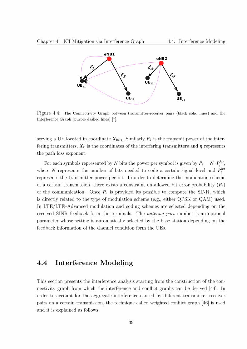
Chapter 4. ICI Mitigation via Interference Graph 4.4. Interference Modeling
Figure 4.4: The Connectivity Graph between transmitter-receiver pairs (black solid lines) and the
Interference Graph (purple dashed lines) [7].
serving a UE located in coordinate XR(i). Similarly Pk is the transmit power of the inter-
fering transmitters, Xk is the coordinates of the interfering transmitters and η represents
the path loss exponent.
For each symbols represented by N bits the power per symbol is given by Pi = N ·Pbiti ,
where N represents the number of bits needed to code a certain signal level and Pbiti
represents the transmitter power per bit. In order to determine the modulation scheme
of a certain transmission, there exists a constraint on allowed bit error probability (Pe)
of the communication. Once Pe is provided its possible to compute the SINR, which
is directly related to the type of modulation scheme (e.g., either QPSK or QAM) used.
In LTE/LTE–Advanced modulation and coding schemes are selected depending on the
received SINR feedback form the terminals. The antenna port number is an optional
parameter whose setting is automatically selected by the base station depending on the
feedback information of the channel condition form the UEs.
4.4 Interference Modeling
This section presents the interference analysis starting from the construction of the con-
nectivity graph from which the interference and conflict graphs can be derived [44]. In
order to account for the aggregate interference caused by different transmitter receiver
pairs on a certain transmission, the technique called weighted conflict graph [46] is used
and it is explained as follows.
39

Chapter 4. ICI Mitigation via Interference Graph 4.4. Interference Modeling
4.4.1 Interference Graph
The IG, G = (V , E), is used to represent the interference among different communi-
cation links (transmitter-receiver pairs) in the network. Where node V represents the
communication links, and the edge E represents the pairwise interference level among
communication links. An example of such graph is represented by a dashed–lines in
Figure 4.4 where lis represent the communication link between an eNB and a specific UE.
To estimate IG, the centralized controller as in Fig. 4.1 should collect the transmis-
sion status of all commuinication links for a certain period of time. In addition, it is
also possible to estimate the IG using micro-probing, which is done by injecting traffic
into the network in order to infer the occurances of interference. Even though micro-
probing is quite accurate, the overhead is very demanding in larger networks. Thus the
choice of which IG estimators to deploy depends on the trade-off between accuracy and
computational complexity.
4.4.2 Conflict Graph Construction
Considering a set of transmitter–receiver pairs {(Xi,XR(i)) : i ∈ N} where Xi and XR(i) rep-
resent the location of the transmitting and receiving terminals respectively. By assuming
a downlink transmission, the connectivity graph can be constructed as a directed graph
from the eNBs (Xi) to the UEs (XR(i)), see Fig. 4.4.
According to the Physical Interference Model [44], in order to have a successful re-
ception at the receiver XR(i), the SINR ≥ β where β is the threshold SINR. Then the
maximum allowed interference level Ii,max at the receiver is calculated as follows.
Ii,max =Pi
β · |Xi − XR(i) |η− σ2 , (4.3)
where Pi represents the transmit power of the eNBs and σ2 is the additive noise power.
The maximum allowable interference contribution of the k-th interfering link (Xk ,XR(k))
on terminal XR(i) is with a fraction of weigth given by (4.4).
wki =
Pk
Ii,max · |Xk − XR(i) |η(4.4)
Sm∑lk
wki ≤ 1 (4.5)
Let li as the communication link between transmitter-receiver pair (Xi,XR(i)), being
represented by a vertex in a weighted conflict graph as in Fig. 4.5. According to the
40

Chapter 4. ICI Mitigation via Interference Graph4.5. Resource Allocation and Optimization
Figure 4.5: Conflict Graph construction [7]
model in [46], there is a weighted edge directed from vertex lk to vertex li with a weight
of wki for i, k ∈ N and i , k. From the weighted conflict graph, which is shown in Fig.
4.5, its possible to determine a set of communication links (i.e., li ∈ Sm) that could be
active at the same time considering the constraint in (4.5) is satisfied. Hence, the links li
∈ Sm can be scheduled at the same time-slot, assuming the aggregate interference caused
by those links is below the allowed maximum interference Ii,max.
4.5 Resource Allocation and Optimization
After constructing the conflict graph, the following step is to come up with a model
that will lower the the weights wki of the conflict graph. For achieving this an efficient
resource-scheduling and or power-allocation technique needs to be adopted. The following
section describes the important parameters that have a direct or indirect impact on the
interference or system performance of the mobile network. Considering a base station
(either macro or small cell) with L transmission links, we can define a set of tunable
parameters that can directly affect the conflict graph. These parameters include: i)
transmission link (UE, eNB) pairs L = {1,2, .., l, ..,L}, ii) resource blocks (frequency, time,
space) R = {1,2, ...,r, ..,R} and iii) modulation and coding schemesM = {1,2, ...,m, ...,M }.
Thus the objective of the optimization problem is to reduce the aggregate interference
on a certain transmission link li, i.e., targeted to reduce the weights of the edges that we
presented in equation (4.4) , or to maximize the SINR at the receiver. Since the weights on
the edges and the interferences created by the interfering links are directly proportional,
equivalently we can minimize the weights by optimizing the power allocation on each
link [47]. The resource allocation problem that results in a reduced weights of the edges
41

Chapter 4. ICI Mitigation via Interference Graph4.5. Resource Allocation and Optimization
of a conflict graph can be formulated as an integer linear problem. Consequently, the
objective function of the optimization problem is given as (4.6a) considering each link li
corresponds to a certain down-link transmission with (transmitter, receiver) pair.
minϕi,k,r,m
L∑i=1
L∑k=1k,i
R∑r=1
M∑m=1
wki,r,m · ϕi,k,r,m (4.6a)
subject to :
L∑k=1k,i
M∑m=1
ϕi,k,r,m ≤ 1 ∀i,r, (4.6b)
M∑m=1
ρi,k,m ≤ 1 ∀i, k, (4.6c)
ϕi,k,r,m ≤ ρi,k,m ∀i, k,r,m, (4.6d)
R∑r=1
M∑m=1
T Pi,k,r,m · ϕi,k,r,m ≥ T Pre fi,k ∀i, k, (4.6e)
ρi,k,m ∈ {0,1} ∀i, k,m, (4.6f)
ϕi,k,r,m ∈ {0,1} ∀i, k,r,m, (4.6g)
Pmin ≤ Pi ≤ Pmax ∀i, k . (4.6h)
Equations (4.6b) to (4.6h) represent the constraint functions for the optimization
problem based on the objective function expressed in (4.6a). ϕi,r,min (4.6g) is a decision
binary variable, which is 1 if link li uses MCS m in RB r or 0 otherwise. Similarly, equation
(4.6f) is also a binary variable that is equal to 1 if link li use MCS m or 0 otherwise.
Considering each eNBs, constraint (4.6b) makes sure that RB r is only assigned to a
single link li at a given time instant (i.e., for links served by the same transmitting eNB;
if the links are in different eNBs then the space component of the RB <time, frequency,
space> makes sure that each RB is assigned to single link), and constraints (4.6c) and
(4.6d) together guarantee that each link is allocated to at most one MCS. Constraint
(4.6e) makes sure that each link achieves its throughput demands T Preqi,k . Finally the last
constraint (4.6h) sets the interval for the possible transmission power level per transmitted
symbol.
The objective function in (4.6a) minimizes the weight wki,r,m by optimizing the alloca-
tion of RBs, transmit power and MCS in the network. The matrix W (defined in eq.
(4.7)), which is a 2-dimentional L×L matrix represents the overall weights associated to
42

Chapter 4. ICI Mitigation via Interference Graph 4.6. Summary
each of the edges of the conflict graph. Each row i in W represents the interference on
each of the transmission links in the presence of L-1 other simultaneous transmissions.
W =
w11 w2
1 w31 . . . wL
1
w12 w2
2 w32 . . . wL
2
w13 w2
3 w33 . . . wL
3
. . . . . . .
w1L w2
L w3L . . . wL
L
(4.7)
where the self-interference term wii= 0. Therefore, minimizing the values of W means
solving the integer programming problem represented by the cost function (4.6a) while
considering the corresponding constraints.
4.6 Summary
In this chapter, a general software-defined based framework for mitigating interfererence
in mobile radio networks is introduced. Using the global view of the network, a central-
ized interference analysis enables an optimized radio resource allocation. A set of mobile
network system parameters ,<time, frequency, space, transmit-power, modulation, coding,
antenna-port>, are abstracted to higher layers in order to improve the programmability
of the network. Moreover, the concept of switch port analogy as it is applied to a wireless
network is presented to further improve the flexibility of choosing the right mapping of
PHY layer system parameters in a centralized manner. In the next chapter, we present
another way of mitigating interference in heterogeneous networks, through fractional fre-
quency reuse technique while applying the SDN concepts.
43

Chapter 4. ICI Mitigation via Interference Graph 4.6. Summary
44

Chapter 5
ICI Mitigation via FFR
5.1 Introduction
To cope with increasing traffic volumes, both academia and industry have started moving
beyond 4G (in other words to 5G networks), where the capacity improvement is expected
to be 1000X [2–4] as compared to the 4G networks. In order to achieve this goal several
different techniques are suggested in the literature [48] such as massive Multiple-Input
Multiple-Output, use of higher frequency spectrum, deploying small cells (i.e., densifica-
tion [49]), traffic offloading, virtualization, control/user plane splitting (i.e., SDN), and
minimization of the functionalities performed by access points. Out of these possible tech-
nologies network densification, deployment of a massive number of small cell base stations,
is the dominant trend, as it is expected to enable network operators to significantly lower
CapEX and OpEX.
Small cells are composed of complex radio units and RRHs. Remote radio heads are
simply equipped with multiple antenna elements and radio front-end and connected to a
remote pool of centralized resources, as in the C-RAN approach [9], through high capacity
and low latency fronthaul connection. The centralized pool of resources are also connected
to the operator’s Evolved Packet Core (EPC) using a high capacity backhaul.
Although densification results in significant system capacity improvement, it also de-
grades the system performance due to the increase in inter cell interference. For example,
in heterogeneous networks where SCs are deployed overlaying macro base stations results
in two kinds of interferences, cross-tier (interference between the MBSs and SCs) and
co-tier (interference among MBSs or among SCs) interfernce, making the interference
management more difficult. FFR is the second example (i.e. followed by IG method
discussed in 4) of interference avoidance technique, which aims to reduce ICI using differ-
45

Chapter 5. ICI Mitigation via FFR 5.1. Introduction
ent frequency reuse techniques for cell-center and cell-edge users, while providing a very
low computational complexity and overhead. In other words, FFR reduces the spectral
efficiency of the network in order to improve the overall SINR of the network. To compen-
sate the loss in spectral efficiency, the selection of the best MCS per transmitted packet
is necessary, which represents an NP-hard problem. An interesting solution is presented
in [50].
In addition, SDN further facilitates the management of ICI of mobile networks in a
flexible manner such that it enables the deployment of a centralized pool of resources or
base band units in a server farm, allowing large deployment of RRHs over space with a
suitable abstraction models. Furthermore, using network functions virtualization, typical
tasks that pertain to MAC and radio resource management can run in virtual machines
and be destined from RRHs. Management of ICI in orthogonal frequency-division multi-
ple access based HetNets is crucial to foster spatial reuse. In addition, another enabler for
5G networks is the non-orthogonal multiple access with successive interference cancella-
tion (SIC) that might replace OFDMA. In [51], the authors proposed an FFR technique
in multiuser non-orthogonal access with SIC to improve the spectral efficiency of a sys-
tem. Thus ICI management can be accomplished with unprecedented flexibility in the
centralized pool of resources in combination with SDN control and NFV.
In this chapter, we propose a centralized and a decentralized resource scheduling al-
gorithm for downlink packets destined to UEs based on the FFR technique, alleviating
interference. In FFR techniques, the frequency band is partitioned in N + 1 sub-bands
with one band for interior users common to all the SCs (i.e. FR1 area) and the remaining
N different bands for the exterior user equipments. Unlike static FFR in which the well
known 1-3 scheme which uses N = 3 bands is adopted for MBSs, we assume that a small
cell coverage area can also be dynamically divided in a different number of sectors to take
into account traffic loads and interference suffered from interior and cell edge users. We
assume that different sectors can be served by different antennas which are physically
connected to the same pool of processing resources. In this way, each sector can be seen
as a separate sub-network implementing its own scheduling rules.
The centralized scheduler is an improvement to the work presented by [50] in terms of
the spectral efficiency and packet blocking probability whereas the decentralized approach
further improves, resource utilization by reducing the probability of dropped packets,
which is an inherent problem introduced by the algorithm (i.e. GAP-Generalized As-
signment Problem) used in [50]. In addition, we implemented the legacy LTE with a
Multi-Choice Knapsack (MCKP) algorithm (with and without power control), in the case
when FFR is not considered and compared the results with both centralized and de-
46
Chapter 5. ICI Mitigation via FFR 5.1. Introduction
centralized approaches. Both the centralized and decentralized approaches contain two
modules: i) the spatial scheduler which runs on a longer time scale, so that its decisions
could be performed from the centralzed controller in the cloud/data center. ii) the MAC
scheduler, which basically resides close to the access points due to the operational time
constraint (e.g., 1ms = 1 transmission time interval in LTE). The MAC scheduler per-
forms the scheduling decisions in a joint manner among all FFR bands (a.k.a SAs), which
is not the case in the decentralized scheduling where each SA runs their own scheduling
algorithm (i.e., MCKP).
The rest of this chapter is organized as follows. Section 5.1.1 describes the related
works in the area. In Section 5.2, the main contributions of our proposed solutions are
presented. The system model and algorithms’ descriptions are described in Section 5.3
and 5.4 respectively. The system analysis of the proposed algorithms are discussed in
Section 5.5. The simulation results are presented in Section 5.6. Finally, Section 5.7
summarizes this chapter.
5.1.1 Related Work
There are several ICI mitigation techniques in the literature. Different power and fre-
quency allocation schemes are deployed to avoid the impact of ICI in cellular networks so
as to improve the system’s spectral efficiency. FFR is the most widely used ICI mitiga-
tion technique, which aims to improve the SINR of the system while fulfilling the transmit
power constraint of an evolved Node B. In FFR the users with a stronger signal qual-
ity (cell-center/internal users) use a lower reuse factor (FR1) and users with lower SINR
(cell-edge/external users) use a higher reuse factor scheme (FR3) [52, 53]. Depending on
the operation time-scale, ICI avoidance schemes are generally categorized as static, semi-
static, and dynamic schemes [24]. In static schemes, the resource block (RB-the smallest
resource unit in LTE-A) allocation for each cell is determined during the radio planning
and it is long-term where the sub-bands assigned to each cell regions are fixed. In semi-
static approaches, the time-scale is in seconds or several hundreds of milliseconds, a part
of the RB allocation is predefined and the other RBs allocations reserved for cell edge
users are dynamically changed. In the dynamic scheme, RB allocation is dynamically
updated depending on the variations of network conditions.
Strict FFR and soft frequency reuse are examples of static frequency techniques. In
[54], Strict FFR technique was presented to obtain a better overall network throughput
and cell-edge user experience as compared to SFR. In one case, the available bandwidth
is partitioned statically in N + 1 sub-bands (Strict FFR) and in the second in N bands
47

Chapter 5. ICI Mitigation via FFR 5.2. Main Contributions
(SFR), which is less efficient in terms of resource utilization. In [55], a dynamic FFR
technique is proposed assuming an asymmetric cell load distribution and using graph
coloring to improve the cell throughput with respect to conventional FFR technique.
Since the approach is based on the conventional static FFR, it cannot fully solve the
inherent inefficiencies in resource utilization.
Even though radio resource scheduling represents a well explored area, it still needs
to be improved to face the ever-growing capacity demand. Fayssal B. et al [56] presented
an evaluation and criticism for different LTE (uplink and downlink) radio resource allo-
cation strategies in the literature. In [50], the authors propose a way to further improve
bandwidth utilization in Static FFR. Indeed, they propose a joint/centralized scheduling
algorithm that includes scheduling decisions for all sectors inside a MBS area. The joint
scheduling is proved to be an NP-hard problem and, in order to solve it in polynomial time,
the authors developed an efficient algorithm with the worst case performance guarantee.
In [50] the partition of bandwidth resources is static across the predetermined cell sectors
or scheduling areas. Moreover, the joint scheduler resides in the MBS, which performs
scheduling in distributed manner resulting in a lower degree of freedom in improving the
overall system interference.
In [27], existing FFR techniques (i.e., Strict FFR, SFR, and FFR-3) are evaluated
in OFDMA-based two-tier (i.e. MBS and SCs) network and a technique called optimal
static FFR is proposed. Optimal static FFR statically partitions the available bandwidth
in seven sub-bands and manually assign different frequency bands to the SCs to mitigate
interference.
5.2 Main Contributions
In this work we propose two approaches to schedule downlink packets in HetNets. In or-
der to relieve ICI, we dynamically partition the SC area in the space domain in different
scheduling areas, thus improving the user exerience of the cell edge users. We formulate
centralized and decentralized scheduling problems which take care of radio resource man-
agement. Both approaches are a combination of two schedulers that operate at different
time scales. On a longer time scale, the spatial scheduler decides how to partition the SC
area, whilst on a finer time scale the MAC scheduler decides the best MCS to use.
The way we devise the scheduling problems provides several advantages over other
approaches available in the literature. Indeed, by dynamically dividing the SC area in
different sectors, we manage to schedule packets in different orthogonal sub-bands using
dynamic Strict FFR, which better adapts to users’ and traffic loads distribution. We
48

Chapter 5. ICI Mitigation via FFR 5.3. System Model
model the coverage area using stochastic geometry, the centralized scheduling problem
in terms of MC-GAP (i.e., Multi-Choise-Generalized Assignement Problem, which is a
combination of MCKP and GAP) and the decentralized scheduling problem in terms
of MCKP. Both MCKP and GAP are two well known NP-hard problems, which can
be solved using efficient approximation algorithms as in [57] and [58], respectively. In
addition, we provide a heuristic centralized scheduling algorithm to further improve the
system performance with a reasonable computational complexity.
Centralization of the radio resources and the intelligence (e.g., spatial scheduler) in the
mobile networks is one of the key enablers for the future wireless networks and beyond.
Our proposed spatial scheduler is a flexible tool used in dense SCs, leaveraging the ab-
straction of the scarce radio resources and the antenna elements of the RRHs. In addition
we present the comparison of MC-GAP and MCKP algorithms as applied to centralized
and decentralized scheduler respectively, in order to study the different degrees of central-
ization with respect to the achieved network perfomance and complexity. This work uses
the comparisons in order to find the right compromise between flexibility, complexity and
performance of our proposed approaches as applied to dense mobile networks.
5.3 System Model
The reference system architecture is shown in Fig. 6.2. The architecture is essentially the
C-RAN, in line with the software-defined RAN architecture defined in [9]. A Cloud BBU
(C-BBU) is made of a central pool of BBU resources in a data center and is physically
connected to several RRHs (RRH Pool). The BBU pool is shared among different cell
sites and this enables to optimize BBU utilization between heavily and lightly loaded
base stations. The crucial issue for this architecture is to provide high capacity and low
latency fronthaul (e.g. to support common public radio interface (CPRI)-the most widely
used interface between RRHs and BBUs) and backhaul connections to ensure that control
decisions are timely delivered to the RAN. For the fronthaul microwave E-band, millimeter
wave or optical fiber serve the purpose. For example, Fujitsu [59] introduced GX4000 an
E-band (operating in the 70/80GHz) radio system, based on an impulse radio technology,
which provides high-speed (up to 3Gbps) transmission, ultra low latency, compact form
factor and low power consumption. The highest percentage of backhaul connections are
done by fiber for small cell deployments WiFi is also seen as a possible solution for wireless
backhauling [60].
The hypervisor (a.k.a. virtualization layer) virtualizes the C-BBU providing an en-
vironment (or in other words, it abstracts the underlying physical network resources)
49

Chapter 5. ICI Mitigation via FFR 5.3. System Model
Figure 5.1: C-RAN system architecture including SDN control and NFV [61].
for the virtualization of the underlying physical network resources. Since the BBU Pool
is shared among different small cell sites and consists of general purpose processors to
perform baseband processing, its functionalities can also be virtualized in a central pool
of resources called virtual BBUs (vBBUs). The SDN controller manages the network
to forward packets from/to the UEs. In addition, it is the one which is reponsible for
triggering the virtual functions to run different optimization algorithms depending on
the information collected from the physical infrastructure. For example, when there is a
congestion in one part of the network, the SDN controller passes a trigger message to the
virtual functions residing in the vBBUs to perform different network optimizing actions
accordingly. vBBUs, are a collection of virtual functions, that enable different operations
such as efficient radio resource allocation, interference and mobility management at the
global network level. The spatial scheduler operates as a virtual network function, is part
of vBBU functions, which lead to more agile network with significant CapEX and OpEX
savings. We remark that the depicted architecture shows the logical connection between
the proposed spatial scheduler and the radio elements, and therefore it is a simplified
version of the architecture shown in [9].
The SINR threshold βFR, the antenna beamwidth θ and the number of antennas can
be selected by the spatial scheduler on a time scale of every 10 ms (i.e., LTE radio frame
- RF), whearas the MCS is decided by the MAC scheduler for each awaiting packet every
1 ms (i.e., transmission time interval). Consequently, we assume that the number of
sub-bands to be used by the schedulers is decided each RF although this time scale of
operation could be even relaxed.
Once the spatial scheduler is implemented and then it is executed in the C-BBU,
50

Chapter 5. ICI Mitigation via FFR 5.4. Algorithm Description
Figure 5.2: The simplified versions of the proposed scheduling approaches.
where different antenna elements can be pooled together and different antenna beamwidth
configurations are selected. In addition, the spatial scheduler is meant to relieve ICI
applying FFR thechnique, dynamically dividing the cell area in different sectors. In each
scheduling areas packets are transmitted with the best MCS selected depending on the
its instantaneous SINR value. Initially, the cell is divided in interior and exterior areas
by dynamically tweaking a suitably defined SINR threshold. Then, depending on the
number of antennas and beamwidth selected, the cell is further divided in sectors. The
interior area is FR1 and the other sectors are denoted by FRn, with n = 1 ÷ N indexing
also the distinct sub-bands.
Other general assumptions include that SC locations are modeled with a homogeneous
Poisson Point Process (PPP) of intensity λ. Based on the PPP assumption, we compute
the probability of coverage using the tool of stochastic geometry in an interference-limited
network under the hypothesis of distant dependent path-loss and Rayleigh distributed
fading. The coverage probability is computed in closed form assuming that ambient noise
can be neglected. For each awaiting packet to transmit we randomly assign a SINR values
corresponding to six different MCSs that we considered. A packet is assumed successfully
received if the instantaneous SINR exceeds the threshold β∗ for detection. After applying
our proposed solutions we assume the ICI problem is solved and that the reception of a
packet is affected only by distance dependent path-loss and Rayleigh distributed fading.
5.4 Algorithm Description
This section describes our approach to the spatial scheduler problem under the different
point of views, the MCKP single bin, MC-GAP, heuristic and MCKP multiple bins. As
it has been discussed in the previous section, in all the cases, first the spatial scheduler
divides the SC area in interior and exterior areas and then into multiple sectors (i.e., which
does not apply in the case of MCKP single bin). The only difference in all the approaches
comes from the fact that they run different algorithms inside the MAC scheduler.
In MCKP single bin we considered the SCs to be equipped with an omnidirectional
antenna, i.e., the scheduling area is one (see Fig. 5.2a). This is the typical LTE-A
51
Chapter 5. ICI Mitigation via FFR 5.5. System Analysis
network with FR1 in overall scheduling area where the MAC scheduler applies the MCKP
algorithm to perform resource scheduling for the packets awaiting for transmission. In
MC-GAP, the SCs contain multiple antenna elements and the cell area is assumed to
be divided into multiple scheduling areas depending on the selected antenna beamwidth
and SINR threshould. MC-GAP is a centralized scheduler running over the multiple
scheduling areas (see Fig. 5.2b). Centralized scheduling improves the spectrum utilization
of the network by scheduling packets to be served in the best scheduling area (by the
best antenna). The only disadvantage related to this algorithm comes from the fact
that how the GAP algorithm works, which is discussed in details in Section 5.6. In
MCKP multiple bins the spatial scheduler, located in vBBU, partitions the SCs area into
a number of sectors and interior and exterior areas. Where each scheduling areas run its
own independent MCKP algorithm, inside the MAC scheduler, to schedule packets (see
Fig. 5.2c). The following section presents the details of each algorithms.
5.5 System Analysis
As briefly highlighted in Section 5.4, we solve the problem of scheduling of downlink pack-
ets in a SC area in two different ways (i.e., centralized and decentralized approaches).
Considering the system architecture in Fig. 6.2, we assume the radio resource manage-
ment (RRM) decisions are taken by the spatial scheduler and MAC scheduler residing
in virtual BBUs and in C-BBUs respectively and distributed to each RRH through the
high performing fronthaul. In this paper, we focus on a reference small cell area which is
divided in different sectors applying dynamic FFR technique to relieve the ICI problem.
The first step is to compute the probability of coverage, which determines the amount of
radio resources assigned for the inner and exterior scheduling areas.
5.5.1 Probability of Coverage
We show a step-by-step computation of the probability of coverage (pc) in cellular net-
works for the downlink. The coverage probability is computed based on the SINR as-
suming that a reference UE makes the attempt to connect to the RRH which transmits
the strongest signal (see Fig. 5.3). In general, UEs may belong to the inner area (FR1
sub-band), while exterior UEs to one of the other scheduling areas (nth sub-band). It is
then the responsibility of the spatial scheduler to assign the UE for instance, e.g., using
MC-GAP algorithm, to a less loaded sector served by another antenna. We define the
SINR as follows
52

Chapter 5. ICI Mitigation via FFR 5.5. System Analysis
Figure 5.3: Distribution of UEs within the selected small cell [61].
γ :=Ptgr−α
Pσ +∑
m Ptmgmr−αm, (5.1)
where r denotes the random variable of the distance between the randomly selected UE
(i.e. reference handheld) and the nearest radio head. Parameter α is the path-loss ex-
ponent, Pt is the transmit power of a RRH, g is the power fading coefficient and rm is
the random distance between the mth interfering SC downlink signal and the reference
UE. Furthermore, gm and Ptm are the fading coefficient and transmit power of the mth
interferer, respectively. Pσ is the ambient noise power. We can now specify pc as the
probability to receive a radio signal above a certain threshold β as follows
pc(λ, β,α
):= EgmErmP(γ > β |rm,gm) , (5.2)
where Egm and Erm represent the expectation with respect to the interfering SCs fading
coefficient gm and distance rm respectively. Relying on [62, 63], we introduce the SINR
threshold βFR to distinguish between packets addressed to UEs in FR1 or FRn areas.
This can be done defining the probability
pFFR := P(γ > β |γ < βFR) , (5.3)
where γ is the SINR of a packet transmitted in one of the N sub-bands after applying FFR.
At first, we compute the coverage probability of an exterior UE since pFFR determines the
size of the scheduling areas in which MC-GAP and the MCKP algorithms are applied.
The probability pFFR was developed for the reference UE in [62, 63] in terms of the
probability pc, which can be written for an interference limited environment in which
noise is neglected (Pσ ≈ 0) as follows
pc(β, λ,α,N ) =1
1 + N−1ρ(β,α), (5.4)
53

Chapter 5. ICI Mitigation via FFR 5.5. System Analysis
with ρ is expressed as
ρ(β,α) = β2/α∫ ∞
β−2/α
1
1 + xα/2dx . (5.5)
The above integral was solved in closed form for α > 2 using Mathematica as follows
ρ(β,α) = β−2/α2π csc( 2πα )
α−2 F1
(1,
2
α,2 + α
α,−β−1
), (5.6)
with 2F1 the hypergeometric function. Then as in [63] pFFR is given by
pFFR =pc(β, λ,α,N )
1 − pc(βFR, λ,α,1)− (5.7)
1
(1 − pc(βFR, λ,α,1))(1 + 2ζ (β, βFR,α,N )),
where ζ (β, βFR,α,N ) =∫ ∞
1
[1 −
1
1 + βFRx−α(1 −
1
N(1 −
1
1 + βx−α))]
xdx . (5.8)
Unlike [62], where pFFR was explicitly provided only for the case α = 4, equation (5.8)
was evaluated in Mathematica for any value of α > 2 and β → βFR as follows
ζ (βFR,α,N ) = (5.9)
βFR2α(1 + βFR)
[−βFR
(2 − 2α + (α − 2)(1 + βFR)
)α − 1
×
2F1(1,2 − 2/α,3 − 2/α,−βFR) + 2(1 +1
N)×(
− 2 + α + 2(1 + βFR)2F1(1, α−2α ,2 − 2α,−βFR))
α − 2
]Therefore, substituting eq. (5.4) and (5.9) in eq. (5.7), we can compute pFFR in a
closed form. Thus, Fig. 5.4 shows the plot of pFFR with respect to SINR threshold,
βFR, for different values of path-loss exponent, α, where larger values of α corresponding
to a higher pFFR distribution. Considering an OFDMA system with bandwidth W and
Nb RBs, the fraction of RBs allocated to the exterior area (Next) depends on the SINR
distribution. Based on the chosen βFR, Next is computed by evaluating the complementary
comulative distribution function (CCDF) of the SINR distribution (i.e., pFFR) at βFR as
follows.
Next = (1 − pFFR(βFR)) × Nb . (5.10)
Depending on the selection of the number of antenna elements and beamwidth θ we shall
assign N = 2π/θ. In this way the amount of RBs in each cell sector for exterior UEs can
be computed as bNext/Nc, where b·c is the highest integer number smaller than bNext/Nc.The remaining RBs are then allocated to the interior UEs, Nint = Nb − Next × N
54

Chapter 5. ICI Mitigation via FFR 5.5. System Analysis
-20 -15 -10 -5 0 5 10 15 20SINR threshold (-
FR) in dB
0
0.1
0.2
0.3
0.4
0.5
0.6
0.7
0.8
0.9
1
Ext
erio
r U
sers
Cov
erag
e P
roba
bilit
y (p
FF
R) , = 2.1
, = 3, = 4
Figure 5.4: The exterior coverage probability with respect to SINR threshold.
5.5.2 Frequency Reuse One (FR1)
The spatial scheduler palys no role in this case, leading to a single scheduling area using
the overall system bandwidth. Since FR1 does not implement any interference reduction
techniques to avoid ICI, it’s performance tightly depends on the antenna transmit power.
In other words, the residual interference in the system depends on the transmit power.
Thus the interference distribution is assumed to be a function of the Rayleigh fading and
the transmit power, which in turn determines the success probability of the transmission.
The details for success probability (ps) derivations could be found in [64,65], but for our
purpose we simplified the experessions (i.e., with and without power control) as follows:
Without Power Control : Considering the uniform PPP distribution of BSs of
intensity λ, with channel access probability of p, SINR threshold β, and with a d dimen-
sional unit ball of volume cd. From [65] ps is given by:
ps = e−λpcdrdE[hδ ]Γ(1−δ) βδ , (5.11)
where δ = d/α, Γ(x) =∞∫0
t x−1e−t dt is a gamma function, and E[hδ] = Γ(1 + δ) is the
expectation of the Rayleigh fading. Using the Γ function identity (i.e., Γ(δ)Γ(1 − δ) =π
sin(πδ) ), d = 2, and cd = π thus (5.11) is simplified as follows.
ps = e−λpπr2
π 2α
sin(π 2α )β2α
, (5.12)
With Power Control : The only difference with respect to the case without power
control is, E[hδ] in (5.11) is replaced by E[hδPtδ], which is simplified as 1
λcdΓ(1 + δ) [64] .
Similarly, the sucess probability simplify to:
55
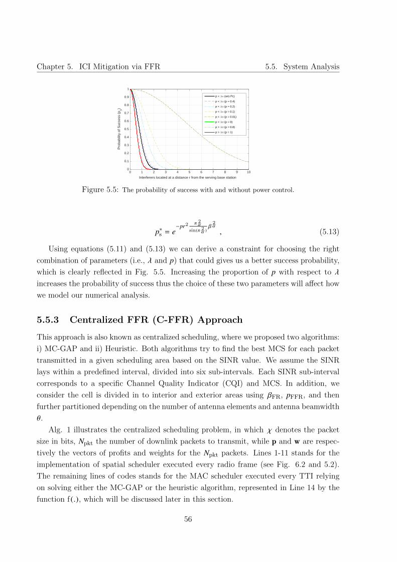
Chapter 5. ICI Mitigation via FFR 5.5. System Analysis
0 1 2 3 4 5 6 7 8 9 10
Interferers located at a distance r from the serving base station
0
0.1
0.2
0.3
0.4
0.5
0.6
0.7
0.8
0.9
1
Pro
babi
lity
of S
ucce
ss (
ps)
p = 6: (w/o Pc)
p < 6: (p = 0.4)
p < 6: (p = 0.2)
p < 6: (p = 0.1)
p < 6: (p = 0.01)
p < 6: (p = 0)
p > 6: (p = 0.8)
p > 6: (p = 1)
Figure 5.5: The probability of success with and without power control.
p∗s = e−pr2
π 2α
sin(π 2α )β2α
, (5.13)
Using equations (5.11) and (5.13) we can derive a constraint for choosing the right
combination of parameters (i.e., λ and p) that could gives us a better success probability,
which is clearly reflected in Fig. 5.5. Increasing the proportion of p with respect to λ
increases the probability of success thus the choice of these two parameters will affect how
we model our numerical analysis.
5.5.3 Centralized FFR (C-FFR) Approach
This approach is also known as centralized scheduling, where we proposed two algorithms:
i) MC-GAP and ii) Heuristic. Both algorithms try to find the best MCS for each packet
transmitted in a given scheduling area based on the SINR value. We assume the SINR
lays within a predefined interval, divided into six sub-intervals. Each SINR sub-interval
corresponds to a specific Channel Quality Indicator (CQI) and MCS. In addition, we
consider the cell is divided in to interior and exterior areas using βFR, pFFR, and then
further partitioned depending on the number of antenna elements and antenna beamwidth
θ.
Alg. 1 illustrates the centralized scheduling problem, in which χ denotes the packet
size in bits, Npkt the number of downlink packets to transmit, while p and w are respec-
tively the vectors of profits and weights for the Npkt packets. Lines 1-11 stands for the
implementation of spatial scheduler executed every radio frame (see Fig. 6.2 and 5.2).
The remaining lines of codes stands for the MAC scheduler executed every TTI relying
on solving either the MC-GAP or the heuristic algorithm, represented in Line 14 by the
function f (.), which will be discussed later in this section.
56
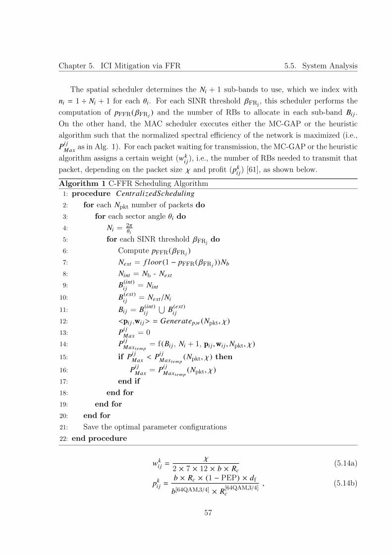
Chapter 5. ICI Mitigation via FFR 5.5. System Analysis
The spatial scheduler determines the Ni + 1 sub-bands to use, which we index with
ni = 1 ÷ Ni + 1 for each θi. For each SINR threshold βFRj, this scheduler performs the
computation of pFFR(βFR j) and the number of RBs to allocate in each sub-band Bi j .
On the other hand, the MAC scheduler executes either the MC-GAP or the heuristic
algorithm such that the normalized spectral efficiency of the network is maximized (i.e.,
Pi jMax as in Alg. 1). For each packet waiting for transmission, the MC-GAP or the heuristic
algorithm assigns a certain weight (wki j), i.e., the number of RBs needed to transmit that
packet, depending on the packet size χ and profit (pki j) [61], as shown below.
Algorithm 1 C-FFR Scheduling Algorithm
1: procedure CentralizedScheduling2: for each Npkt number of packets do
3: for each sector angle θi do
4: Ni = 2πθi
5: for each SINR threshold βFRjdo
6: Compute pFFR(βFR j)
7: Next = f loor (1 − pFFR(βFR j))Nb
8: Nint = Nb - Next
9: B(int)i j = Nint
10: B(ext)i j = Next/Ni
11: Bi j = B(int)i j
⋃B(ext)
i j
12: <pi j ,wi j> = Generatep,w (Npkt, χ)13: Pi j
Max = 0
14: Pi jMaxtemp
= f (Bi j , Ni + 1, pi j ,wi j ,Npkt, χ)
15: if Pi jMax < Pi j
Maxtemp(Npkt, χ) then
16: Pi jMax = Pi j
Maxtemp(Npkt, χ)
17: end if
18: end for
19: end for
20: end for
21: Save the optimal parameter configurations
22: end procedure
wki j =
χ
2 × 7 × 12 × b × Rc(5.14a)
pki j =
b × Rc × (1 − PEP) × df
b[64QAM,3/4] × R[64QAM,3/4]c
, (5.14b)
57

Chapter 5. ICI Mitigation via FFR 5.5. System Analysis
where b and Rc are the number of bits/symbol and the code rate of the selected MCS
to transmit the packet respectively. The factor 2 × 7 × 12 represents that number of
symbols/PRB where LTE PRB occupying 2 slots (1 slot = 0.5ms = 6/7 OFDM symbols
depending on the size of the cyclic prefix-CP) by 12 sub-carriers. PEP represents the
radio channel packet error probability. b[64QAM,3/4] and R[64QAM,3/4]c represent the number
of bits and coding rate for the best possible MCS selection and df is the fraction of packet
payload excluding overhead. Thus the two algorithms, either MG-GAP or heuristic,
replacing the function f (·) in Line 14 of Alg. 1 are described as follows.
MC-GAP algorithm: MC-GAP is the combination of two well known NP-hard
problems MKCP and GAP. MCKP tries to find the best MCS for each packet transmitted
in a single scheduling area based on the corresponding SINR value. Whereas GAP tries
to schedule a packet in a any of the scheduling areas which gives the best profit. An
efficient polynomial time approximations for MCKP and GAP is presented in [57] and
[58] respectively. In addition the detials of this algorithm can be found in our previous
work [61].
Heuristic algorithm: this algorithm is proposed in a quest for improving the per-
formance of the MC-GAP algorithm with a reasonable computational complexity. The
operation of the heuristic algorithm is explained using the following example. Let us con-
sider 3 scheduling areas (a.k.a. bins) in the network each having a radio resource capacity
of B1 = 15 RBs, B2 = 10 RBs and B3 = 9 RBs respectively. We also consider three differ-
ent configurations in sending any packet (a.k.a. item) in a given scheduling area with the
corresponding number of RBs required (item size or weight-wki j) and an associated profit
(pki j). The tables in Fig. 5.6 represent the weight-configuration and profit-configuration
pairs in each bin corresponding to each packet to be transmitted.
The first step is to find the configuration that gives us the best profit in each bin for
each item. Corresponding to the selected configuration we also mark each item’s size from
the weight-configuration table. This step is described in tables as shown in Fig. 5.7 using
the light silver color. Form these tables, the thick black boxes show the configuration
of each item that leads to the best profit out of all possible configurations in different
bins and their corresponding weights. Now, we check if each bin’s capacity constraint is
satisfied. In order to do that we add all the weights of each packet k corresponding to
the selected configuration in each bin and compare them against the corresponding bin
sizes (i.e., [B1 B2 B3] = [15 10 9]). The sum of weights packing items 3 and 4 in bin 1 is
4 + 12 = 16 > B1, similarly for bins 2 and 3 it is given by 3 < B2 and 3 < B3 respectively.
The corresponding sum of profits for the corresponding packing is 25 + 36 + 30 + 32 =
123. However the constraint for bin 1 does not hold, that means we have to find another
58
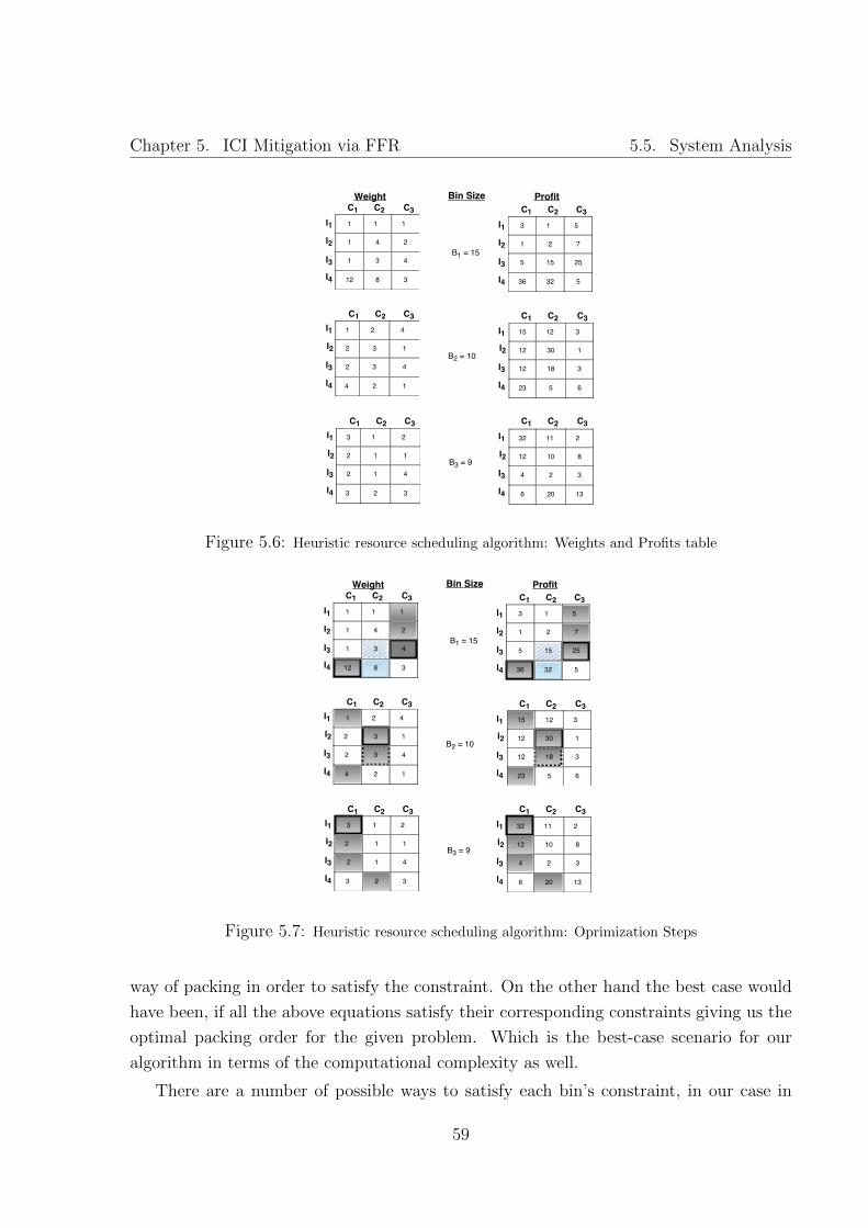
Chapter 5. ICI Mitigation via FFR 5.5. System Analysis
Figure 5.6: Heuristic resource scheduling algorithm: Weights and Profits table
Figure 5.7: Heuristic resource scheduling algorithm: Oprimization Steps
way of packing in order to satisfy the constraint. On the other hand the best case would
have been, if all the above equations satisfy their corresponding constraints giving us the
optimal packing order for the given problem. Which is the best-case scenario for our
algorithm in terms of the computational complexity as well.
There are a number of possible ways to satisfy each bin’s constraint, in our case in
59

Chapter 5. ICI Mitigation via FFR 5.5. System Analysis
bin 1. In bin 1, we first check for the next best profit with a lower weight for either
item 3 or 4. We start changing the configuration of item 3 in bin 1 to configuration 2
(shown in blue right slanted pattern) with a bin size of 3 and profit 15 while keeping the
configuration of item 4 unchanged. Then we compare for the best way of packing item
3 with a given profit from the remaining bins (bin 2 gives us the best profit-as shown
in blue right slanted pattern rectangle). In this case all the bin capacity constraints are
satisfied, 12 < B1, 3 + 3 < B2 and 3 < B3. The overall profit of packing all the items in
all the bins becomes 36 + 30 + 18 + 32 = 116.
Then the next step is to check if we can further improve the profit while only changing
the configuration of item 4 while keeping item 3 in bin 1 with configuration 3. First
let us change the configuration of item 4 from configuration 1 to 2 (shown in blue left
slanted pattern), which gives us a lower profit and a lower weight. Then we check if this
profit in bin 1 is better than the other bins, which is the case. Then we check if bin 1’s
constraint is satisfied with the new configuration for item 4 (i.e., 4 + 8 = 12 < B1). The
new profit using this configuration becomes 25+32+30+32 = 119. Thus this gives us the
optimal packing of the packets (i.e., [I1, C1, B3], [I2, C2, B2], [I3, C3, B1] and [I4, C2, B1])
complying while satisfying each bin’s size constraint. However this might not be the case
all the time, we might not able to reach to the optimal solution as fast as this. In such
cases we settle for a sub-optimal solution with a reasonable computational complexity.
The heuristic algorithm does not enforce the hard constraint on the bin sizes as in
MC-GAP algorithm. It initially finds the best profit for every item in each bin without
any consideration to the bin size constraint. Then it checks for the fulfillment of each
of the bin size constraints, this relaxation enables to achieve a better performance as
compared to MC-GAP.
5.5.4 Decentralized FFR (D-FFR) Approach
In this approach, the spatial scheduler divides the cell in to sectors, interior and exterior
scheduling areas. Where each scheduling areas runs the MCKP algorithm independently
and concurrently at the MAC scheduler.
The main difference of this approach (i.e., Alg. 2) as compared to Alg. 1 is line
14 of Alg. 1 is replaced by line 15 in Alg. 2. The MCKP(.) algorithm is executed
simultaneously in each scheduling areas based on the MCKP algorithm running in the
MAC scheduler as shown from line 15 to line 22 in Alg. 2. The lines of codes from line
15 to line 22 are supposed to be executed conccurently in each scheduling area, whereas
for readability purpose we presented in Alg. 2 the sequential version of it. Line 23 saves
60

Chapter 5. ICI Mitigation via FFR 5.5. System Analysis
all the optimal parameters (i.e., maximum profit, optimal beamwidth and optimal SINR
threshold) so that further analysis will be done.
The difference between the centralized and decentralized scheduling approachs is re-
flected in terms of their computational complexity and their corresponding system perfo-
mance (discussed in the results section).
Algorithm 2 D-FFR Scheduling Algorithm
1: procedure DecentralizedScheduling2: for each Npkt number of packets do
3: for each sector angle θi do
4: Ni = 2πθi
5: for each SINR threshold βFRjdo
6: Compute pFFR(βFR j)
7: Next = f loor (1 − pFFR(βFR j))Nb
8: Nint = Nb - Next
9: B(int)i j = Nint
10: B(ext)i j = Next/Ni
11: Bi j = B(int)i j
⋃B(ext)
i j
12: for each bin ni do
13: <pi j ,wi j> = Generatep,w (Npkt, χ)14: Pi j
Max = 0
15: Pi jMaxtemp
= MCKP (Npkt, χ,Bnii j , Ni + 1, pi j ,wi j )
16: if Pi jMax < Pi j
Maxtemp(Npkt, χ) then
17: Pi jMax = Pi j
Maxtemp(Npkt, χ)
18: end if
19: end for
20: end for
21: end for
22: end for
23: Save the optimal parameter configurations
24: end procedure
5.5.5 Computational Complexity Comparison
Both MCKP and GAP algorithms being NP-hard problems, there is a need to approximate
them efficiently with a polynomial-time algorithm.
61

Chapter 5. ICI Mitigation via FFR 5.6. Results
Definition: A polynomial-time approximation scheme (PTAS) is a family of al-
gorithms Aε , where there is an algorithm for each ε > 0, such that Aε is a (1 + ε )-approximation algorithm (for minimization problems) or (1− ε )-approximation algorithm
(for maximization problems). Thus the approximation algorithm Aε has a absolute per-
fomance guarantee or bounded error ε , i.e., (OPT-ε) ≤ Aε ≤ (OPT+ε). Where OPT
represents the optimal solution obtained by the optimal algorithm.
In [57] a fully polynomial-time approximation scheme (FPTAS) is proposed for MCKP
(i.e., the algorithm used in decentralized FFR scheduling approach) algorithm. The pro-
posed algorithm runs in O(|K | |C |/ε
)time where |K | is the number of packets waiting to
be transmitted and |C | is number of different MCSs. Since the MC-GAP algorithm uses
MCKP algorithm, its running time depends on that of the MCKP algorithm. Thus the
running time for MC-GAP becomes O(|B | f
(|K |, |C |
)+ |B | |K | |C |
)where |B | represents the
number of sub-bands (scheduling areas) and f(|K |, |C |
)is the running time of the MCKP
algorithm. In the case of heuristic algorithm, the computational complexity varies from
O(|K | |B |
)in a best case to O
(|K |2 |C | |B |
)in the worst case. As the number of packets
to be transmitted, |K |, increases the running time for both centralized and decentralized
scheduling approaches converge to the same value.
5.6 Results
We evaluated the performance of the proposed (i.e., legacy LTE, centralized, and decen-
tralized) scheduling algorithms using numerical simulations. The general setup for the
simulations is based on the system model persented in Section 5.3 and the detailed anal-
ysis carried out in Section 5.5. We assumed a UE is served by the nearest BS where the
BSs in the network are distributed with PPP of intensity λ, which in turn accounts the
amount of inteference introduced by the neighbouring BSs. We run simulations increasing
the number of packets waiting for transmission in downlink, thus increasing the network
traffic load. For each number of packets, the MC-GAP and MCKP algorithms are exe-
cuted as described in sub sections 5.5.3 and 5.5.4 respectively. Packets are generated at
the beginning of each radio frame and they are scheduled every TTI. The computation of
the weight and the profits for each packet is shown in eq. 5.14a and 5.14b respectively.
The profit is computed taking into account the effect of coding, overhead and PEP. The
packet overhead df is assumed fixed, whereas the coding rate changes depending on the
MCS selected along with the number of bits b.
Since both the centralized and decentralized approaches are assumed to mitigate ICI,
then the probability of accepting/rejecting a packet at the receiving UE solely depends
62

Chapter 5. ICI Mitigation via FFR 5.6. Results
on the noise. Thus the test for accepting/rejecting is based on comparing the PEP,
a value randomly generated between zero and one, with a threshold value. Hence, we
compute the packet success probability (ps) assuming distance dependent path-loss and
Rayleigh fading as in (5.15). However for the case of the fequency reuse one approach (as
in Section 5.5.2), we used the expressions in (5.12) and (5.13) without and with power
control respectively.
ps = P(SNR > β) = exp
(−
β
Ptrα
), (5.15)
where SNR is the signal-to-noise-ratio. Hence, a packet is rejected if the PEP is greater
than 1 − ps and accepted otherwise. The remaining part of this section is subdivided in
to two sub-sections. Sub-section 5.6.1 introduces the possible key performance indicator
(KPI) parameters used for our analysis and the numerical results are presented in sub-
section 5.6.2.
5.6.1 Performance Metrices
In this section, we provide the definitions of the possible key performance indicators that
we choose to evaluate our proposed algorithms.
Def.1 Packet Blocking Probability : it is the ratio between the number of dropped
(Nd) to the number of packets awaiting transmission (Nt). Where Nd is defined as the
difference between Nt to the number of packets successfully transmitted (N st ) considering
enough resource allocation in scheduling area, i.e., Nd = Nt - N st . Nd is mainly affected
by the proportion of the radio resources allocated in the SAs, i.e., its directly related to
pFFR.
Def.2 Normalized Spectral Efficiency (η∗): this is the number of useful bits
which can be achieved per transmitted packet with respect to the best possible MCS. It
also depends on the selected MCS and code rate, the packet overhead and the loss of
packes due to the radio channel (the expression is exactly the same as the one given by
(5.14b)) as shown below.
η∗ =b × Rc × (1 − PEP) × df
b[64QAM,3/4] × R[64QAM,3/4]c
, (5.16)
Def.3 Aggregate Throughput (T P∗Agg): - is just the summation of all the optimal
profits of the transmitted packets obtained by the proposed schedulers and it is expressed
as follows
63

Chapter 5. ICI Mitigation via FFR 5.6. Results
T P∗Agg = b[64QAM,3/4] × R[64QAM,3/4]c × N f
168
TT I
K∑k
η∗k (5.17a)
T P∗Agg = N f168
TT I
K∑k
(bk × Rk
c × (1 − PEPk ) × df), (5.17b)
where b[64QAM,3/4] and R[64QAM,3/4]c are denormalizing factors. N f represents the minimum
number of RBs needed to transmit a particular packet of size χ bits using the best
MCS selection in a particular transmission time interval (i.e., 1ms). For example, for
transmiting a packet of size 128 bytes (χ = 128bytes) we need 2 RBs (i.e., N f = 2). The
number 168, 2 × 7 × 12, is the factor that we used in (5.14a) representing the number
of resource elements (RE) (i.e., 1RE = 1 OFDM duration × 1 OFDM sub-carrier) in an
LTE subframe (1ms).
Def.4 Optimal Beamwidth (θ∗): - is the optimal beamwidth that maximizes the
performance (i.e., the aggregate TP or the normalized spectral efficiency) of the network.
In other words the beamwidth that maximizes the profit of the MC-GAP or MCKP
algorithms for the centralized and decentralized scheduling algorithms respectively.
Def.5 Optimal Beta (β∗): - similar to θ∗, it is the SINR theshold that maximizes
the performance of the network.
5.6.2 Numerical Results
Simulations were carried out in MATLAB environment with numerical parameters shown
in Table 5.1. We assumed an LTE system bandwidth of W = 20MHz and results are
provided for the packet size of 32, 128 and 256 bytes. In addition, we considered two
different ranges of β corresponding to the two path-loss exponents, α = 2.1 and 4. The
reason is that, for example considering α = 2.1 there are cases where we have a zero radio
resource allocation in some bins/SAs that limits us from performing any optimization.
Every TTI a different number of packets are scheduled for transmission and for each packet
the profit and weight are computed based on the CQI value. The CQI values depend on
the SINR, which are randomly generated and could fall within any of the six SINR sub-
intervals (see Table 6.1). For every TTI the MC-GAP and the MCKP algorithms are
executed to find the most suitable MCS for transmitting packets in the different Ni+1
sub-bands. A number of simulation rounds were conducted to obtain a statistical average
of the key performance indicators defined in Section 5.6.1.
64

Chapter 5. ICI Mitigation via FFR 5.6. Results
Table 5.1: System parameter settingParameter Value
System Bandwidth W = 20 MHz
Packet Size (χ) 32, 128, and 256 Bytes
Transmit Power (Pt) 46 dBm
α 2.1 and 4
λ 0.15
β [-10 5] dB for α = 2.1
[-5 10] dB for α = 4
θ [9001200]
MCS [r, Rc ] [QPSK, 1/2], [QPSK, 3/4], [16QAM, 1/2]
[64QAM, 1/2], [64QAM, 2/3], [64QAM, 3/4]
SINR ranges [dB] 0 − 6.5, 6.5 − 7.2, 7.2 − 13.6
13.6-18, 18 − 21, 21 − 25
df 0.75
p 0.2
Number of observations 50
0 50 100 150 200 250 300 350
Number of Generated Packets
0
0.1
0.2
0.3
0.4
0.5
0.6
0.7
0.8
0.9
1
Blo
ckin
g P
roba
bilit
y
Static MG-GAP: , = 2.1Static MG-GAP: , = 4MC-GAP: , = 2.1MC-GAP: , = 4MCKP-Multiple Bins: , = 2.1MCKP-Multiple Bins: , = 4MCKP-Single Bin-w/oPC: , = 2.1MCKP-Single Bin-w/oPC: , = 4MCKP-Single Bin-wPC (p=0.2): , = 2.1MCKP-Single Bin-wPC (p=0.2): , = 4Heuristic: , = 2.1Heuristic: , = 4
Figure 5.8: Packet blocking probability Vs the number of generated packets for χ = 32 bytes and α =
2.1 and 4.
Fig. 5.8 shows the packet blocking probability versus the number of packets generated,
i.e., the traffic load, every TTI. It can be clearly seen that the best case, lowest blocking
probability, is for the MCKP single bin (i.e., FR1) scenario with or without power control.
On contarary, the state-of-the-art (Static MC-GAP) [50] performing bad and the MC-
GAP (centralized scheduler) and MCKP with multiple bins (decentralized scheduler)
lying in between. The reason for the MCKP with a single bin to have the lowest blocking
probability is that, it tries to schedule any packet as long us there is a RB in the scheduling
area (which is a single SA having all the available resources). The only reason to drop
packets is when all of the radio resources are exhausted, which is not the case for MC-GAP
and MCKP with multiple bins. In both approachs the scheduling of packets depend on
65

Chapter 5. ICI Mitigation via FFR 5.6. Results
0 50 100 150 200 250 300 350
Number of Generated Packets
0
0.5
1
1.5
2
2.5
Spe
ctra
l Effi
cien
cy
MCKP-Single Bin-wPC (p=0.2): , = 2.1MCKP-Single Bin-wPC (p=0.2): , = 4MCKP-Single Bin-wPC (p=0.4): , = 2.1MCKP-Single Bin-wPC (p=0.4): , = 4MCKP-Single Bin-wPC (p=0.8): , = 2.1MCKP-Single Bin-wPC (p=0.8): , = 4MCKP-Single Bin-w/oPC: , = 2.1MCKP-Single Bin-w/oPC: , = 4
Figure 5.9: Spectral efficiency (with and without power control) Vs the number of generated packets
for χ = 32 bytes and α = 2.1 and 4.
the availability of RBs in each scheduling area, since we have more than one scheduling
area consisting of smaller number of RBs, if a packet ends up in a loaded SA the chance of
being dropped increases. In similar argument to the MCKP single bin case, the blocking
probability of the heuristic algorithm performs identically. As long as there is free radio
resource in any of the bins, the heuristic algorithm also tries to transmit a packet in that
bin.
Another interesting thing to see from this plot, changing the path-loss exponent (α)
and introducing a power control doesn’t affect the blocking probability for MCKP with a
single bin. But for MCKP with mutiple bins and MC-GAP changing α affects the blocking
probability, α controls the coverage probabilty (eq. (5.7)) which inturn determines how
the RBs should be partitioned (eq. (5.10)) among the SAs. As reported in [61], increasing
the packet size χ increases the blocking probability since the test for accepting the packets
depends on the number of RBs needed to transmit the packet, the larger the packet size
the more RBs that it needs. Moreover, the packet blocking probabilies of MCKP with
multiple bins is predominantly affected by the way we parition the radio resources across
the SAs than by the packet error rate at reception, which is clearly seen from the fact
that the blocking probability for α = 4 is better than the one for α = 2.1.
Figs. 5.9 and 5.10 represent the spectral efficiency (i.e., the number of bits needed to
transmit a symbol) of the network versus the number of generated packets for a packet
size of χ = 32 bytes. In Fig. 5.9 we can see the effect of selecting different power control
parameter (p as reported in eq. (5.13)) in MCKP-Single Bin algorithm. Considering
p = 0.2 for both α = 2.1 and 4 gives a better performance as compared to other values of
66

Chapter 5. ICI Mitigation via FFR 5.6. Results
0 50 100 150 200 250 300 350
Number of Generated Packets
0
0.5
1
1.5
2
2.5
3
3.5
Spe
ctra
l Effi
cien
cy
Static MC-GAP: , = 2.1Static MC-GAP: , = 4MC-GAP: , = 2.1MC-GAP: , = 4MCKP-Multiple Bins: , = 2.1MCKP-Multiple Bins: , = 4Heuristic: , = 2.1Heuristic: , = 4
Figure 5.10: Spectral efficiency Vs the number of generated packets for χ = 32 bytes and α = 2.1 and
4.
0 50 100 150 200 250 300 350
Number of Generated Packets
0
10
20
30
40
50
60
Thr
ough
put [
Mbp
s] Static MC-GAP: , = 2.1Static MC-GAP: , = 4MC-GAP: , = 2.1MC-GAP: , = 4MCKP-Multiple Bins: , = 2.1MCKP-Multiple Bins: , = 4MCKP-Single Bin-w/oPC: , = 2.1MCKP-Single Bin-w/oPC: , = 4MCKP-Single Bin-wPC (p = 0.2): , = 2.1MCKP-Single Bin-wPC (p = 0.2): , = 4Heuristic: , = 2.1Heuristic: , = 4
Figure 5.11: Aggregate throughput Vs the Number of generated packets for χ = 32 bytes α = 2.1 and
4.
p. On the other hand, when we increase the value of p to 0.8, we can see the case without
power control out performs the one with power control (this is clearly justified by Fig.
5.5).
From Fig. 5.10 we can see that MCKP with multiple bins out performs all the other
approaches except the heuristic algorithm. MC-GAP algorithm have low spectral effi-
ciency due to the high packet blocking probability as reported in Fig. 5.8. In all the cases
except the heuristic and MC-GAP algorithm, the performance for α = 4 is better than
for α = 2.1. This is due to the fact we used a different range of SINR thresholds for α =
2.1 and 4 when implementing the MC-GAP algorithm. Since MC-GAP algorithm have
some constraints (i.e., the inherent characterstics of the GAP algorithm) in dividing the
67

Chapter 5. ICI Mitigation via FFR 5.6. Results
0 50 100 150 200 250 300 350
Number of Generated Packets
0
10
20
30
40
50
60
Thr
oupu
t [M
bps]
Static MC-GAP: 32 BytesStatic MC-GAP: 128 BytesStatic MC-GAP: 256 BytesMC-GAP: 32 BytesMC-GAP: 128 BytesMC-GAP: 256 BytesMCKP-Multiple Bins: 32 BytesMCKP-Multiple Bins: 128 BytesMCKP-Multiple Bins: 256 BytesHeuristic: 32 BytesHeuristic: 128 BytesHeuristic: 256 Bytes
Figure 5.12: Aggregate throughput Vs the Number of generated packets for variable transmission
packet size: α = 2.1.
2 6 10 14 18 22 30 40 50 70 100 150 200 275 350
Number of Generated Packets
0
20
40
60
80
100
Fre
qunc
y of
Occ
uran
ce o
f 3* in
(%
)
3 = 900
3 = 1200
Figure 5.13: Histogram of θ∗ Vs the Number of generated packets of C-FFR scheduler for χ = 32 bytes
and α = 4.
proportions RBs in a SAs, we opt to use different ranges of the SINR. In general, for α
= 4 we expect a better performance as compared to α = 2.1 which is the case as shown
in Fig. 5.10. Due to possibility of allocating RBs to a packet in any of the less loaded
SAs, the spectal efficiency of the heuristic algorithm is not affected by the choice of the
path-loss exponent, α.
Figs. 5.11 and 5.12 represents the aggregate throughput of the system for different
values of the path-loss exponents and variable packet sizes respectively. From Fig. 5.11 the
decentralized approach out performs the centralized (i.e., MC-GAP) approaches and α = 4
gives a better performance as compared to α = 2.1 except for MC-GAP for the same reason
as explained above. Whereas the heuristic algorithm, which is a centralized scheduling
algorithm out performs all providing a superior aggregate throughput for the considered
path-loss exponents. As it can be clearly seen in Fig. 5.12 increasing the transmitted
68

Chapter 5. ICI Mitigation via FFR 5.6. Results
0 2 6 10 14 18 22 30 40 50 70 100 150 200 275 350Number of Generated Packets
0
10
20
30
40
50
60
70
80
90
100
Fre
qunc
y of
Occ
uran
ce o
f 3* in
(%
) 3 = 900
3 = 1200
Figure 5.14: Histogram of θ∗ Vs the Number of generated packets of D-FFR scheduler for χ = 32
bytes and α = 4.
packet size decreases the aggregate throughput of the network as the consequence of an
increase in packet blocking probability.
The histograms of the optimal beamwidth selection θ∗ over the number of observations
for the centralized and decentralized scheduling algorithms are reported in Figs. 5.13 and
5.14 respectively. From Fig. 5.13 we can easily see the optimal θ∗ to be 90◦ for lower
traffic loads and becomes 120◦ as the traffic load increases. Thus increasing the size of
the SAs, i.e., the number of RBs in each SA, improves the performance of the network.
In contrast, for the decentralized scheduler (see Fig. 5.14) increasing the traffic load has
a different effect. For a lower traffic loads θ∗ = 120◦ but for higher traffic loads there
are circumstances where θ∗ = 90◦ is also selected. On the other hand, for the heuristic
algorithm (the results are not presented here due to the space constraint) considering the
two path-loss exponents, α = 2.1 and 4, θ∗ = 90◦ for all traffic loads.
Fig. 5.15 represents the optimal SINR threshold β∗ over the possible round of simu-
lations. To make a better sense of the result we computed the weighted mean of β∗ over
the number of observations as follows.
β∗ =
Q∑q=1
β∗qωq
Q∑q=1
ωq
, (5.18)
where β∗q represents the optimal SINR threshold for one observation and ωq represents
the weight or the frequency of the same SINR threshold chosen as an optimal value.
In the case of MC-GAP algorithm, for α = 4 the bigger the SINR threshold (β) the
better the performance is, i.e., more radio resources are allocated to exterior users than
69

Chapter 5. ICI Mitigation via FFR 5.7. Summary
0 50 100 150 200 250 300 350
Number of Generated Packets
-10
-5
0
5
10
15
Wei
ghte
d M
ean -
* (dB
)
MCKP-Multiple Bins: , = 2.1MCKP-Multiple Bins: , = 4MC-GAP: , = 2.1MC-GAP: , = 4Heuristic: , = 2.1Heuristic: , = 4
Figure 5.15: Weighted mean β∗ ( β∗) Vs the Number of generated packets for transmission packet size
of: χ = 32 bytes.
the interior users in order to reduce the effect of the interference. Instead for α = 2.1
more radio resources are allocated for the interior users than the exterior users. Thus
the radius of the interior coverage area of α = 2.1 is larger than of α = 4. Similarly, for
heuristic algorithm when α = 2.1 more radio resources are allocated for the interior users
and for α = 4 more radio resources are allocated to the exterior users. In addition, for the
heuristic algorithm the optimal SINR threshold, β∗, tends to stablize after the traffic load
reaches 100 packets (i.e., the maximum number of packets that the system can handle).
In decentralized scheduling the change in the path-loss exponent does not have a
significant change in the selection of the optimal SINR threshold (β∗) value. In both
cases the the SINR threshold tends to minimize as the traffic load increases leading to
more resource allocation to the interior users than the exterior once.
5.7 Summary
In this chapter we proposed two scheduling approaches (i.e., centralized and decentralized)
based on the FFR technique, to mitigate the ICI in small cell networks. Each approaches
consist of two schedulers operating in different time scales. Depending on the traffic load
in the small cell, the spatial scheduler dynamically changes the antenna beamwidth to
partition the cell area in different sectors every LTE radio frame. Whereas the MAC
scheduler operating in a short time scale executes every TTI. The joint scheduling prob-
lem is formulated by a combination of MCKP and GAP approximation algorithms and
the decentralized approach is formulated as a knapsack problem. Furthermore, we tackled
the problem of modeling the cell coverage using a stochastic geometry. Numerical results
have shown that our proposed approaches out performs the state-of-the-art for the same
70

Chapter 5. ICI Mitigation via FFR 5.7. Summary
network conditions. Our approach could also be extended for the future generation net-
works (i.e., 5G networks and beyond) where non-orthogonal multiple access is proposed
as a replacement for the OFDMA.
Up until now, we have been discussing about how to mitigate ICI in cellular networks.
However, the next part (i.e. Part III) of this dissertation will focus on resource slicing
in wireless networks using both the SDN and NFV paradigms for enabling efficient radio
resource utilization of a wireless network.
71

Chapter 5. ICI Mitigation via FFR 5.7. Summary
72
Part III
Resource Slicing in Wireless
Networks


Chapter 6
Spectrum-level Slicing
6.1 Introduction
Network programmability and virtualization are key enablers of the flexibility and adapt-
ability required in future wireless networks. Network virtualization enables network oper-
ators to share the same physical infrastructure and have networks coexisting in a flexible
and dynamic manner. Thus allowing a customized network services and efficient resource
utilization [66, 67]. Wireless network virtualization enables efficient resource utilization
through dynamically sharing the physical wireless infrastructure among different mobile
network operators. In addition to sharing the wireless infrastructure, it also enables the
sharing of radio spectrum resources in order to reduce the capital and operational expen-
ditures (i.e., CapEX and OpEX) [31,32] of the network.
In this chapter we focus on one aspect of network virtualization: efficient management
of virtual radio resources. The HetNets used in this work are based on a LTE technology
where the base stations are connected to the evolved packet core through the S1-interface.
The virtual radio resource pool is an abstraction of physical radio resources, i.e., the time,
frequency and space (base station) dimensions available for supporting communications
in a given HetNets. As shown in Fig. 6.1, each HetNet contains a number of high-power
and low-power BSs, also known as MBSs and SCs respectively. The virtualization layer
is responsible for mapping the physical radio resources to a central virtual radio resource
pool (VRRP). Such different virtual resources (e.g., virtual antenna elements, virtual
baseband processing units, etc.) are combined together to create a virtual network. A
virtual network operates similar to a traditional network with fixed physical resources
and it does not necessarily have any awareness of the underlying physical infrastructure
associated with its resources. These VNs are owned by MNOs, which are responsible
75
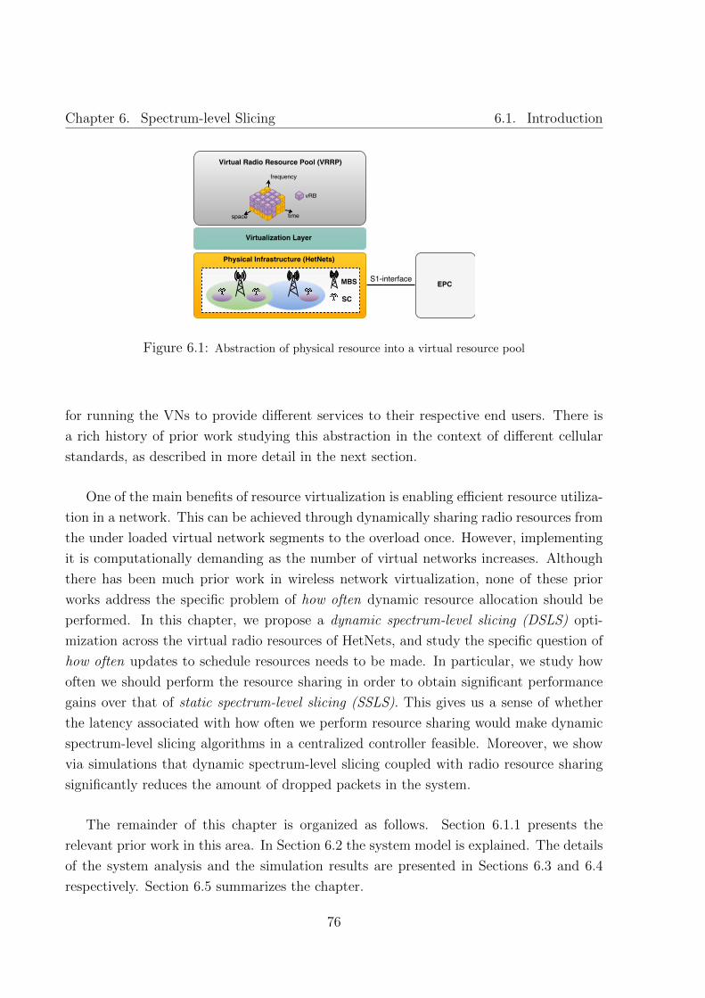
Chapter 6. Spectrum-level Slicing 6.1. Introduction
Figure 6.1: Abstraction of physical resource into a virtual resource pool
for running the VNs to provide different services to their respective end users. There is
a rich history of prior work studying this abstraction in the context of different cellular
standards, as described in more detail in the next section.
One of the main benefits of resource virtualization is enabling efficient resource utiliza-
tion in a network. This can be achieved through dynamically sharing radio resources from
the under loaded virtual network segments to the overload once. However, implementing
it is computationally demanding as the number of virtual networks increases. Although
there has been much prior work in wireless network virtualization, none of these prior
works address the specific problem of how often dynamic resource allocation should be
performed. In this chapter, we propose a dynamic spectrum-level slicing (DSLS) opti-
mization across the virtual radio resources of HetNets, and study the specific question of
how often updates to schedule resources needs to be made. In particular, we study how
often we should perform the resource sharing in order to obtain significant performance
gains over that of static spectrum-level slicing (SSLS). This gives us a sense of whether
the latency associated with how often we perform resource sharing would make dynamic
spectrum-level slicing algorithms in a centralized controller feasible. Moreover, we show
via simulations that dynamic spectrum-level slicing coupled with radio resource sharing
significantly reduces the amount of dropped packets in the system.
The remainder of this chapter is organized as follows. Section 6.1.1 presents the
relevant prior work in this area. In Section 6.2 the system model is explained. The details
of the system analysis and the simulation results are presented in Sections 6.3 and 6.4
respectively. Section 6.5 summarizes the chapter.
76

Chapter 6. Spectrum-level Slicing 6.1. Introduction
6.1.1 Prior Work
In 2008 J. Sachs and S. Baucke introduced the concept of radio virtualization [67], which
is the process of sharing and allocating radio resources across different networks (typically
belonging to different MNOs). In particular, they introduced a resource pooling strategy
for code-division multiple access (CDMA) such that all the radio resources from each base
station are pooled together across a 3-dimensional (3D) resource pool of time, frequency,
and code and then sliced among virtual radio resources. The case study conducted in [36]
extended the concepts of radio virtualization to LTE cellular networks. In the proposed
LTE architecture for radio virtualization, based on a priori information (e.g., channel
conditions), the hypervisor (responsible for mapping the physical radio resources to VNs)
schedules the air interface resources between virtual evolved node Bs; the physical re-
sources of the eNBs are scheduled among different virtual instances via the hypervisor.
In addition, the authors considered slicing of the physical resource blocks corresponding
to a single eNB into multiple virtual eNBs.
In [30] WiMAX BS radio resources are virtualized and assigned to multiple MNOs.
These radio resource are allocated in two different ways, resource-based and bandwidth-
based. In resource-based allocation, a fraction of a BS’s resource slot per orthogo-
nal frequency-division multiple access frames is allocated for a given MNO, while in
bandwidth-based allocation the resource is allocated in terms of the aggregate throughput
(in Mbps) it provides. The authors formulated the resource allocation problem using a
utility-based optimization.
Another relevant work by A. Gudipati et al. [68] proposed a scheme to dynamically slice
3D radio resources (i.e., time, frequency, space) according to the traffic load and service
agreements between the MNOs. In [69] a wireless resource virtualization framework was
proposed, where the problem was formulated as a binary integer programming (BIP)
problem for a single eNB. In [42] Luisa et al. proposed a scheme for adaptive radio resource
allocation for virtual resources abstracted from a heterogeneous wireless infrastructure,
where a BS is virtualized into multiple virtual BSs and these virtual BSs are allocated to
a certain VN; a capacity demand increase in one of the VNs then leads to allocation of the
additional resource required from the other coexisting VNs (a set of VNs participating
in a predefined resource sharing agreement among themselves) based on a pre-defined
contract.
Our work is different from the existing once in terms of: i) proposing dynamic vir-
tual radio resource sharing among coexisting VNs in HetNets, ii) investigating how often
resource sharing should be performed in relation to the achievable network perfromance
77

Chapter 6. Spectrum-level Slicing 6.2. System Model
Figure 6.2: The system model
gain and the feasibility of implementing the dynamic resource sharing functionality far
from the physical infrastructure, and iii) considering an adaptive modulation and coding
scheme in order to accurately estimate the amount of radio resources needed in each VN.
6.2 System Model
In this section we describe the system model for performing dynamic spectrum-level slic-
ing. Fig. 6.2 shows the functional view of the system, which is composed of different
modules, each responsible for handling different roles. As will be discussed later in this
chapter, while our system model is specific to LTE, the dynamic resource allocation algo-
rithms we propose can be applied to general cellular systems with pooled radio resources.
In our system model the virtual resource controller (VRC) is responsible for making dif-
ferent decisions based on the global view of the network. It contains two modules: the
virtual radio resource pool and the slice manager (see Fig. 6.2). The VRRP is an abstrac-
tion of the radio resources of the HetNets. It is a 3D pool of resources, which consists
of <time, frequency, space>. The <time, frequency> dimensions represent the orthogo-
nal frequency-division multiplexing resource blocks in LTE, while the <space> dimension
represents the serving BS. We also define the smallest unit of a virtual radio resource as
a virtual RB (vRB), which is a < time, f requency, space > slot. A slice is a collection
of these virtual RBs, which is allocated to a certain VN. We consider 2 VNs (VN1 and
VN2), purple and orange colored as shown in Fig. 6.2, corresponding to the slices of
virtual radio resources in the VRRP. We have a total of NRB vRBs in the system, i.e. in
the VRRP.
When one of the VNs is overloaded, i.e., it cannot support its current traffic, the slice
manager is triggered. This in turn triggers the dynamic spectrum-level slicer to dynami-
cally share available virtual radio resources among the two VNs based on a preset sharing
78
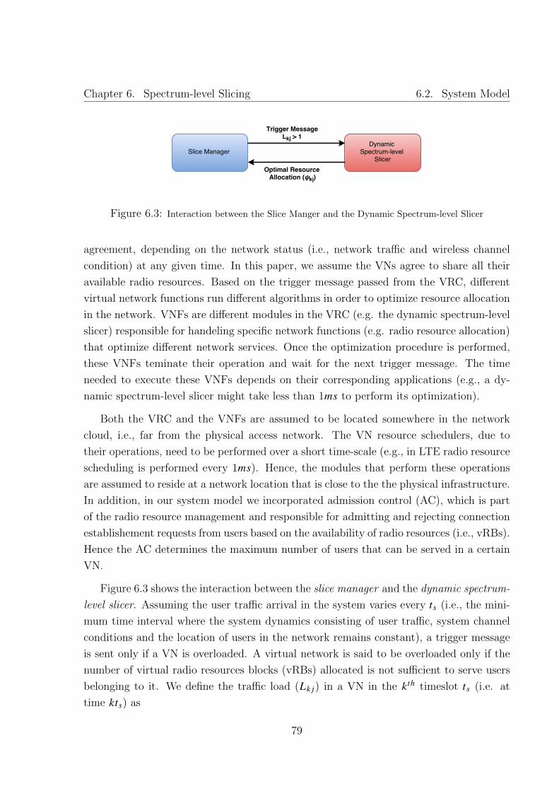
Chapter 6. Spectrum-level Slicing 6.2. System Model
Figure 6.3: Interaction between the Slice Manger and the Dynamic Spectrum-level Slicer
agreement, depending on the network status (i.e., network traffic and wireless channel
condition) at any given time. In this paper, we assume the VNs agree to share all their
available radio resources. Based on the trigger message passed from the VRC, different
virtual network functions run different algorithms in order to optimize resource allocation
in the network. VNFs are different modules in the VRC (e.g. the dynamic spectrum-level
slicer) responsible for handeling specific network functions (e.g. radio resource allocation)
that optimize different network services. Once the optimization procedure is performed,
these VNFs teminate their operation and wait for the next trigger message. The time
needed to execute these VNFs depends on their corresponding applications (e.g., a dy-
namic spectrum-level slicer might take less than 1ms to perform its optimization).
Both the VRC and the VNFs are assumed to be located somewhere in the network
cloud, i.e., far from the physical access network. The VN resource schedulers, due to
their operations, need to be performed over a short time-scale (e.g., in LTE radio resource
scheduling is performed every 1ms). Hence, the modules that perform these operations
are assumed to reside at a network location that is close to the the physical infrastructure.
In addition, in our system model we incorporated admission control (AC), which is part
of the radio resource management and responsible for admitting and rejecting connection
establishement requests from users based on the availability of radio resources (i.e., vRBs).
Hence the AC determines the maximum number of users that can be served in a certain
VN.
Figure 6.3 shows the interaction between the slice manager and the dynamic spectrum-
level slicer. Assuming the user traffic arrival in the system varies every ts (i.e., the mini-
mum time interval where the system dynamics consisting of user traffic, system channel
conditions and the location of users in the network remains constant), a trigger message
is sent only if a VN is overloaded. A virtual network is said to be overloaded only if the
number of virtual radio resources blocks (vRBs) allocated is not sufficient to serve users
belonging to it. We define the traffic load (Lk j) in a VN in the kth timeslot ts (i.e. at
time kts) as
79
Chapter 6. Spectrum-level Slicing 6.3. System Analysis
Lk j =
I j∑i=1
niRBk j
ψ(k−1) j, (6.1)
where j ∈ {1,2} represents the VN index, I j is the number of UEs in VN j, ψ(k−1) j
represents the number of vRBs allocated for VN j in ts (k − 1) and niRBk j
is the number
of vRBs needed to transmit a packet destined to UE i in VN j in timeslot kts. niRBk j
is
computed based on the channel conditions (i.e., determines the right MCS to use) and
users’ data rate (i.e., the number of bits to be transmitted in the ts time interval). Based
on the channel state, captured by the SINR, there is an associated MCS that determines
the number of bits per symbol used to transmit a particular packet which in turn dictates
the number of vRBs needed for the transmission. Then the dynamic spectrum-level
slicer computes the optimal radio resource allocation, ψk j , based on the solution to the
optimization problem defined in Section 6.3.1 for each VN j at timeslot kts. Sub section
6.3.2 provides a detailed analysis of the dynamic spectrum-level slicer.
In the case of static spectrum-level slicing, whose performance we will compare against
that of our dynamic method, the two modules depicted in Fig. 6.3 are missing from the
system architecture shown in Fig. 6.2 (i.e., ψk j is fixed, for example to NRB
2 for both
VNs; there is no sharing of radio resources among the VNs). The outputs of the dynamic
spectrum-level slicer, ψk j , are then fed to each VN so they can independently execute their
own MAC layer resource scheduling algorithms based on the available resources assigned
to them from the slicer (e.g., proportional fair, round robin, etc.). Based on the available
vRBs in each VN j in time interval ts (i.e., ψk j), the MAC schedulers (see Fig. 6.2)
allocate these resources for each user traffic belonging to VN j.
6.3 System Analysis
The dynamic spectrum-level slicer algorithm, the system traffic model and the key pre-
formance indicators are discussed in subsections 6.3.1, 6.3.2 and 6.3.3 respectively.
6.3.1 Dynamic spectrum-level slicer
Upon receiving the trigger message (see Fig. 6.3) from the VRC, this module executes
the dynamic spectrum-level slicer algorithm. The trigger message is sent due to a traffic
overload in any of the coexisting VNs, i.e., Lk j > 1. The operations of the dynamic
spectrum-level slicing algorithm is explained as follows.
80

Chapter 6. Spectrum-level Slicing 6.3. System Analysis
At the begining, in the first timeslot ts, we equally allocate the avialable number of
vRBs for each VN (i.e., ψ0 j ←NRB
2 ). Then we monitor the network traffic load every ts
and check whether the traffic load in VN j exceeds the amount of vRBs allocated to it
in timeslot kts. Whenever a traffic overload happens, (Lk j > 1), in any of the coexisiting
VNs the sliceOptimizer procedure will be executed.
The sliceOptimizer procedure takes the following inputs: a utility function (Usys), a
set of linear constraints (C) and the number of vRBs needed to satisfy the users traffic
(ψestk j =
I j∑i=1
niRBk j
) depending on the variable channel condition using an adaptive MCS for
each packet awaiting to be transmitted in VN j in timeslot kts and outputs the optimal
resource allocation ψk j ← sliceOptimizer(Usys,C,ψestk j ). There is no specific rule for the
type of utility function to choose but, as a general rule, the function that we choose should
follow the law of diminishing returns. This captures the fact that the satisfaction level of
each UE belonging to a certain VN saturates in long run, i.e., no matter how many vRBs
we allocate to a given UE, its satisfaction tends to saturate. In this work we considered
two different utility functions.
Uk j = ln(ψk j ) (6.2)
Uk j =ψk j
1 + ψk j, (6.3)
where Uk j is the utility function of VN j and ψk j is the number of vRBs allocated for VN
j in timeslot kts. Thus, considering the utility function (6.2), the system utility function
becomes: Usys =∑
j ln(ψk j ). The sliceOptimizer solves the optimization problem based
on the following objective function and a list of linear constraints, C.
maximizeψk j
∑j
νk j ln(ψk j ), j ∈ {1,2}, k ∈ N
subject to∑
j
ψk j = NRB,
ψestk j ≤ ψk j ,
ψk j ≥ 0.
(6.4)
where ψestk j represents the amount of vRBs needed to satisty the current traffic and it is
computed in the same way for both static and dynamic spectrum-level slicing algorithms,
and νk j is a scaling factor that multiplies the proportions of each radio resource allocated
for each VN. In our analysis νk j is the estimated achievable spectral efficiency (i.e., the
81

Chapter 6. Spectrum-level Slicing 6.3. System Analysis
amount of bits transmitted in VN j over a time interval ts using a certain bandwidth f )
of a VN j in timeslot kts, which is computed as
νk j = 2 ×
I j∑i=1
niRBk j
× pik js × T BSi
k j
ts × f, (6.5)
where pik js is the packet success probability (i.e., the ratio of successfully delivered packets
to the transmitted ones or pik js = P(SINRikj > β) where SINRikj represents the instanta-
neous SINR of a packet destined to user i belonging to VN j in timeslot kts and β is the
SINR threshold value for the detection of a packet at the receiving user), and TBSikj is the
transport block size (i.e., the number of bits transmitted per ts using a particular MCS
and number of vRBs) of a packet destined to UE i. In the LTE ts = 1ms and f is the
bandwidth occupied by one vRB ( f = 180KHz). In LTE standard, the transport block
size values are determined based on a predefined mapping table that maps a particular
MCS index to a particular TBS.
This convex optimization problem, eq. (6.4), can easily be solved using available opti-
mization packages (e.g., [70]). The constraints and the objective function are explained in
Section 6.4. The output of this optimization problem is the optimal vRBs allocation (i.e.,
ψk j) for each VN where, based on this allocation scheme, each VN independently runs
its own MAC resource scheduler (i.e., represented by resourceScheduler(ψk j) procedure)
every ts.
6.3.2 User Traffic Model
This section focuses on the system user traffic model. We considered the network system
setting shown in Fig. 6.4, which contains five total BSs: two MBSs and three SCs, with
UEs served by these BSs. The number of UEs at each time interval ts are assumed to be
distributed according to a Poisson distribution [P(X = x) =λxm j e
−λmj
x! , where λm j is the
mean of the distribution and m ∈ {1,2, ...,M } represents the serving BS index for UEs in
slice j where M = 5].
We assume the system dynamics, the channel quality (i.e. the SINR), the user equip-
ment locations (assumed to be uniformly distributed), and the network traffic variations
(i.e. the number of UEs in the network) changes every ts (see Fig. 6.5). From Fig. 6.5,
the network monitoring events correspond to checking the network state every ts and
the count of these events is represented by a variable Nsim. Similarly, variations in the
network traffic are assumed to occur every ts, the count of these events is given by Ntraffic
(i.e. the number of timeslots that the network traffic variations have occured). If there is
82
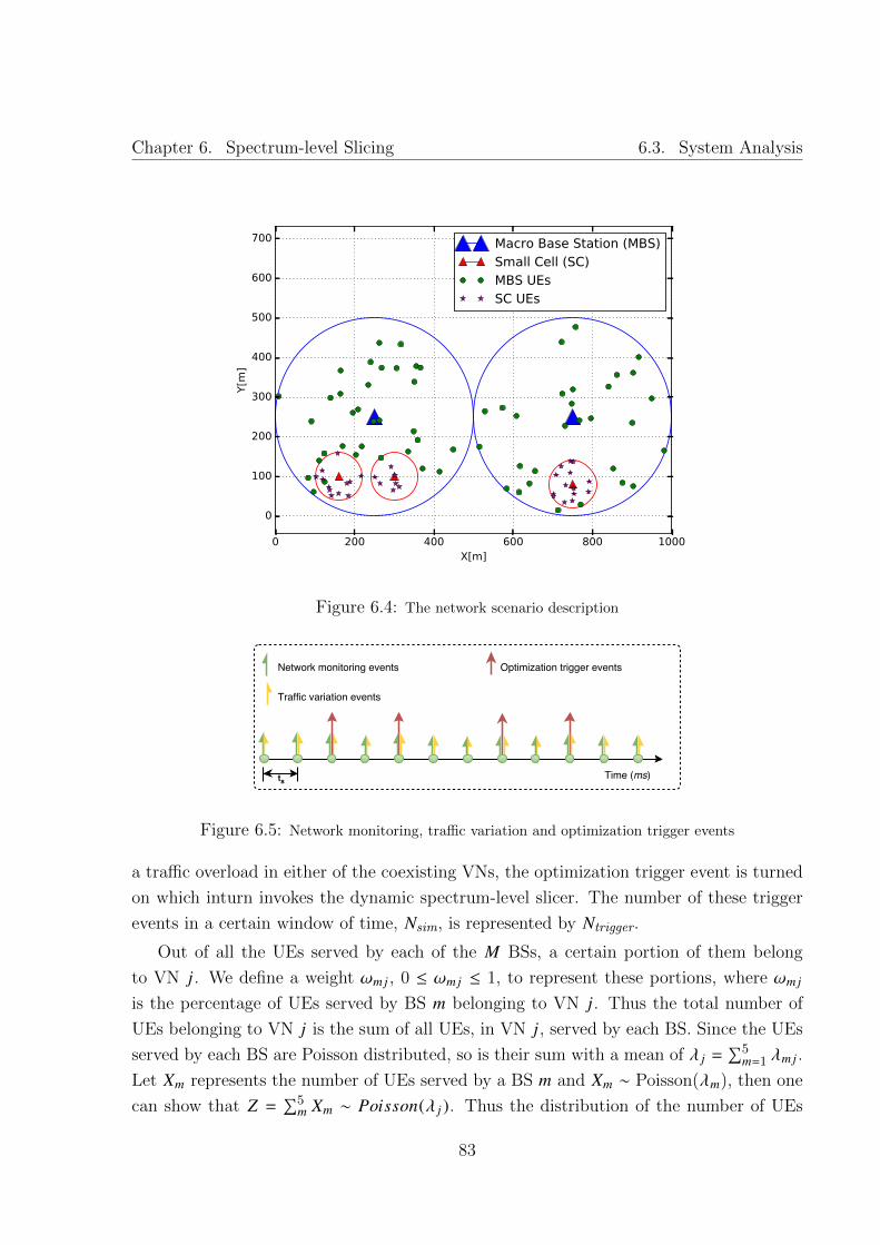
Chapter 6. Spectrum-level Slicing 6.3. System Analysis
0 200 400 600 800 1000X[m]
0
100
200
300
400
500
600
700Y[m
]Macro Base Station (MBS)Small Cell (SC)MBS UEsSC UEs
Figure 6.4: The network scenario description
Figure 6.5: Network monitoring, traffic variation and optimization trigger events
a traffic overload in either of the coexisting VNs, the optimization trigger event is turned
on which inturn invokes the dynamic spectrum-level slicer. The number of these trigger
events in a certain window of time, Nsim, is represented by Ntrigger.
Out of all the UEs served by each of the M BSs, a certain portion of them belong
to VN j. We define a weight ωm j , 0 ≤ ωm j ≤ 1, to represent these portions, where ωm j
is the percentage of UEs served by BS m belonging to VN j. Thus the total number of
UEs belonging to VN j is the sum of all UEs, in VN j, served by each BS. Since the UEs
served by each BS are Poisson distributed, so is their sum with a mean of λ j =∑5
m=1 λm j .
Let Xm represents the number of UEs served by a BS m and Xm ∼ Poisson(λm), then one
can show that Z =∑5
m Xm ∼ Poisson(λ j ). Thus the distribution of the number of UEs
83

Chapter 6. Spectrum-level Slicing 6.3. System Analysis
belonging to VN j is given by
P[Z = zk j ] = λzk jj
e−λ j
zk j !. (6.6)
Similarly, the sum of two weighted Poisson distributions ω1 j X1 + ω2 j X2 with a mean
of λ1 j and λ2 j is also a weighted Poisson distributed with a mean of λ j = ω1 jλ1 j +ω2 jλ2 j .
As in eq. (6.6) we can generalize the weighted sum distribution of M random variables
having a mean of λ1 j , λ2 j , ..., λM j and the corresponding weights ω1 j ,ω2 j , ...,ωM j as
P[Z = zk j ] =( M∑
m=1
λm jωm j) zk j e
−M∑
m=1λmjωmj
zk j !. (6.7)
Both equation (6.6) and (6.7) are defined without the consideration of AC in the
system. Later in this section the effect of implementating AC will be explained. Assuming
zk j is the total number of UEs in slice j in timeslot kts, the computation of the optimization
problem (referred in eq. 6.4) occurs only if zk j > ψ(k−1) j . Since our system’s dynamics
(zk j) change every ts, see Fig. 6.5, zk j follows a weighted Poisson distribution. Due to
the implementation of AC, the system only admits UEs until all the available vRBs are
allocated. Thus, the once which were not admitted should be excluded from the considered
distribution. Let zk j represent this new user distribution after admission control with a
distribution given by P[Z = zk j ] = P[Z = zk j |zk j≤NRB2
] =P[Z=zk j ]
P[zk j≤NRB2 ]
. Therefore the new user
distribution becomes
P[Z = zk j ] =( NRB
2∑s=0
λsje−λ j
s!
)−1λ
zk jj
e−λ j
zk j !, (6.8)
where λ j =M∑
m=1λm jωm j . Once we have the user distribution, the next step is to define the
perfomance indicators that we use to evaluate our simulations.
6.3.3 Key Performance Indicators
We consider two performance indicators: i) the percentage of optimization events (%optEvents)
and ii) the percentage of dropped packets (%droppedPkts).
%optEvents is the ratio between the number of optimization events (Ntrigger) with
respect to the number of traffic variation events (Ntraffic). The network is assumed to be
84

Chapter 6. Spectrum-level Slicing 6.4. Numerical Results
monitored for a total of Nsim × ts secs (see Fig. 6.5), where Ntrigger ≤ Ntraffic ≤ Nsim. In
this work we assumed an independent traffic variation every ts, i.e., Ntraffic = Nsim. Hence
%optEvents =Ntrigger
Ntraffic× 100 , (6.9)
where the number Ntrigger corresponds to how often we perform optimization, depending
on both how fast the network conditions are changing and how many total vRBs are
available in either of the VNs. If the network traffic becomes more than the available vRB
in either VN following the network traffic variation (i.e. Ntrigger ' Ntraffic), every traffic
variation leads to performing optimization operation, in which case %optEvents → 100%.
This makes it harder to implement virtual functions in a centralized way. On the other
hand, if it so happens that the number of traffic variation events are statistically less
frequent, then implementing the virtual function in a centralized way is may be feasible.
%droppedPkts is the difference between the number of dropped packets in static
spectrum-level slicing (NSSLSdropped
) and dynamic spectrum-level slicing (NDSLSdropped
) algorithms
divided by the total number of transmitted packets (Ntx) and expressed as
%droppedPkts =NSSLS
dropped− NDSLS
dropped
Ntx× 100. (6.10)
This perfromance indicator represents the performance improvement in the system
adopting our proposed algorithm with respect to the static-spectrum level slicing algo-
rithm, i.e., no spectrum sharing is allowed among the coexisting virtual networks.
6.4 Numerical Results
We use the system setting given in Fig. 6.4 in order to validate our proposed algorithm.
Table 6.1 gives the details of the simulation parameter settings for heterogeneous system,
as it is defined in [71]. In order to solve the optimization problem given in eq. (6.4),
we applied the algorithm in [70] called constrained minimization of multivariate scalar
functions. In addition, the simulations are based on an LTE network where ts is replaced
by a corresponding term called transmission time interval, which is the smallest time
interval (1ms) where BSs schedule radio resources to users.
Considering an LTE network, every TTI a number of downlink packets of size 32 bytes
are scheduled for transmission which are associated with the two VNs. Depending on the
SINR of the UEs, for each packet destined to these UEs we associate a channel quality
indicator. We considered 15 different SINR intervals corresponding to 15 CQIs, where each
85

Chapter 6. Spectrum-level Slicing 6.4. Numerical Results
Table 6.1: System parameter settingsParameter Value
System layout 5 omnidirectional BSs
System Bandwidth W = 20 MHz
Operating frequency 2GHz
Resource Partitioning Proportional fair
Noise PSD −174dBm/Hz
Shadowing σ = 8dB
Noise figure 9dB
Penetration Loss 20dB
MSB transmit power 46dBm
SC transmit power 37dBm
MBS antenna gain 15dBi
SC antenna gain 5dBi
Beam pattern gain 0dBi (ominidirectional antenna)
3GPP path loss model for MSB PL(r ) = 128.1 + 37.5 · log r1000
3GPP path loss model for SC PL(r ) = 140.7 + 36.7 · log r1000
Table 6.2: UE concentration in each VNType of BSs % UEs in VN1 % UEs in VN2 λ-MT λ∗-HT
MBS1 90% 10% 40 40
MBS2 15% 85% 30 35
SC1 85% 15% 9 12
SC2 90% 10% 10 13
SC3 25% 75% 12 15
CQI maps to a particular MCS that can be supported for the considered transmission. In
addition, based on the CQI information and the number of vRBs allocated per transmitted
packet, we determine the TBS of each packet.
A number of simulation rounds (i.e., 1 simulation round = 100 TTIs = 10 radio
frames (RFs)) were conducted to obtain a statistical average of the key performance
indicators: %optEvents and %droppedPkts. The proportion of UE concentration (ωm j)
served by different BSs belonging to each VN is given by Table 6.2. Each BS is assumed
to serve an independent number of UEs drawn from a Poisson distribution every TTI.
The amount of traffic handled by each BS is controlled by the proper selection of the UE
intensity (λ), which is the mean of the Poisson distribution. In this simulation we used
two different traffic loads, moderate and high, which are represented in Table 6.2 by λ
and λ∗ respectively.
Fig. 6.6 shows the percentage of optimization events (%optEvents) happening from
the round of simulations that we conducted. For evey round (i.e., 10RFs) of simulations
we counted how often the VRC sends the optimization trigger message to the DSLS.
From the results it can be seen that the percentage of optimization events is 40% and
60% on average for both utility functions and traffic loads considered (i.e., solid lines
86

Chapter 6. Spectrum-level Slicing 6.4. Numerical Results
5 10 15 20Round of Simulations (1 round = 10RFs)
0
20
40
60
80
100
Perc
enta
ge o
f O
pti
miz
ati
on E
vents
(%optEvents
)
U(ψkj) =ψkj/(1 +ψkj)− (MT)
U(ψkj) = ln(ψkj)− (MT)
U ∗ (ψkj) =ψkj/(1 +ψkj)− (HT)
U ∗ (ψkj) = ln(ψkj)− (HT)
Figure 6.6: The percentage of an optimization event occurrence
1 2 3 4 5 6 7 8 9 10RF index (1RF = 10 TTIs)
0
2
4
6
8
10
Perc
enta
ge o
f D
ropped P
ack
ets
(%droppedPkts
)
U(ψkj) =ψkj/(1 +ψkj)− (MT)
U(ψkj) = ln(ψkj)− (MT)
U ∗ (ψkj) =ψkj/(1 +ψkj)− (HT)
U ∗ (ψkj) = ln(ψkj)− (HT)
Figure 6.7: The average percentage of dropped packets in SSLS (i.e. conventional scheme) with respect
to our proposed algorithm
indicating moderate traffic (MT)-λ and dashed lines indicating high traffic (HT)-λ∗) in
the network. This is because for approximately half of the times traffic was varied, the
resources allocated for each VN were enough to accommodate the corresponding change
in traffic (i.e., Lk j < 1). Consquently, the results show on average the system solves the
optimization problem every 2 TTIs for both moderate and high traffic loads.
Fig. 6.7, with solid lines indicating moderate traffic-MT and dashed lines indicating
87

Chapter 6. Spectrum-level Slicing 6.5. Summary
high traffic-HT, shows the percentage of dropped packets (%droppedPkts) due to the lack
of radio resources in either of the VNs if we only adopt the SSLS with respect to DSLS.
A significant amount of packets destined to the UEs are dropped every RF in the case
of the conventional SSLS, where the lack of sharing of vRBs among the VNs leads to a
degradation in system performance. In both Fig. 6.6 and 6.7, the two utility functions
perform without any significant difference. Due to the advantages obtained from the
global view of the network, dynamically sharing radio resources among VNs significantly
improves the network performance as compared to the conventional static allocation.
6.5 Summary
We have proposed a dynamic spectrum-level slicing technique for HetNets for dynamically
allocating resources to virtual networks from a virtual radio resource pool. Numerical
results have shown our proposed approach outperforms the static spectrum-level slicing
by reducing the number of dropped packets. The proposed technique is not limited to
LTE, it can also be applied to different radio access technologies. Future developments
will focus on providing a more realistic user traffic model and accurately computing the
inter-arrival time between successive optimization trigger events to determine latency
constraints on the optimization procedure. We will also investigate the scalability issues
of our proposed approach in relation to an increase in the number of VNs in the system.
In the next chapter, we are going to discuss about the techniques for enabling an
end-to-end slicing in wireless networks. Radio resource slicing that we discussed in this
chapter is one of the important ingredients to enable radio access network slicing, which
is one of the requirements for towards an E2E network slicing.
88

Chapter 7
E2E Network Slicing
7.1 Introduction
Current mobile networks are optimized to serve only mobile phones. However, in the 5G
era and beyond, they will be required to serve a variety of devices with heterogeneous
quality of service requirements. The 5G infrastructure public private partnership [72]
classified these services into three use cases, each having different QoS requirements; i)
massive broadband: to deliver gigabytes of bandwidth to mobile devices on demand, ii)
massive machine type communication, also known as massive Internet of Things-IoT:
targeted to connect immobile sensors and machines, and iii) critical machine-type com-
munication: to allow immediate feedback with high reliability in cases like autonomous
driving, remote controlled robots. Although the terminologies are different, these three
categories of communications defined in two organizations as shown in Table 7.1 imply
that 5G mobile networks must support very different QoS for each type of communica-
tions, thus addressing the requirements for supporting extreme flexibility in 5G mobile
networks.
In order to support the above services, it is very costly and impractical to make a
separate dedicate network to provide the required QoS. The most attractive and efficient
solution in terms of reducing cost while improving backward compatibility is through
the implementation of service-dedicated virtual networks [72,73] and [12], a concept also
known as network slicing. Through network slicing it is possible to achieve flexible and on
demand service-oriented network deployments. Software-defined networking and network
function virtualization are the two main enabling technologies in creating network slices
on a single physical network infrastructure (resource). In [74], the standardization effors of
extending SDN and virtualization to wireless networks for enabling an end-to-end network
89

Chapter 7. E2E Network Slicing 7.1. Introduction
slicing is presented.
Table 7.1: 5G use case examples and their QoS requirements [72]5G Use Cases Examples Requirements Mobility
xMBB 4K/8K ultra high definition High capacity, video cache Yes
(UHD) video, hologram,
Augmented Reality (AR),
Virtual Reality (VR)
mMTC Sensor Networks (smart Massive connection No
metering, logistics, city, covering a very large area
home, etc.) of mostly immobile devices
uMTC Autonomous driving, smart Low latency and high Yes
-grid, remote surgery reliability
The rest of this chapter is organized as follows. Section 7.1.1 describes an end-to-end
network slicing. In Sections 7.2 and 7.3 EPC and RAN slicing are presented respectively.
An OpenAirInterface based RAN slicing prototype is described in Section 7.3.1. The
implementation of dynamic spectrum-level slicing based on an OAI experimental testbed
is discussed in Section 7.3.2. Section 7.4 summarizes the chapter.
7.1.1 E2E Network Slicing
Although the concept of network slicing for mobile networks is relatively new in the
technology world today, it is rapidly gaining momentum as we proceed into the future.
5GMF network architecture committee led by the authors of this paper has identified the
importance of end-to-end network slicing, all the way from UE to cloud data centers for
enabling end-to-end quality and extreme flexibility to accommodate various applications,
as shown in Fig. 7.1 included in the white paper [75].
Fig. 7.1 captures two significant aspects of E2E network slicing. First, down at the
bottom, we have physical infrastructure, that is, a collection of network, computing and
storage resources, all the way along E2E communication. We should be able to use these
programmable resources embedded along the E2E communication paths. Second, we
should be able to logically define an E2E network slice from UE to cloud data centers
using the programmable resources per application service. This means that we need to
enable dynamic create, modify and destroy a network slice, coordinated especially across
fixed network and radio boundary, so called mobile packet core slicing and radio access
network slicing.
Depending on the level of virtualization, each network slice is made up of a virtualized
air-interface, radio access network and mobile packet core network and transport network
or combination of these virtual resources. We also note that mobile fronthaul (MFH) and
90

Chapter 7. E2E Network Slicing 7.2. Evolved Packet Core Slicing
Figure 7.1: End-to-end slicing for 5G systems [75]
mobile backhaul (MBH) network slicing need to be considered as well. In the following
sections, we focus our discussion on the techniques of virtualizing evolved packet core and
radio access network.
7.2 Evolved Packet Core Slicing
Performance is an important factor to be considered in programmable 5G networks, which
is highly dependent on the underlying hardware infrastructure. Hardware EPC appliances
can achieve high performance but may lack flexibility in changing their functions once the
logic has been programmed. To balance the flexibility and performance, we choose multi-
core network processors as the platform to prototype the data-path of the EPC slice. In
this section, we introduce how to implement an EPC slice in a FLARE [76] slice shown
in Fig. 7.3, where signaling related EPC entities (e.g., MME) are implemented in control
plane while user data forwarding and processing (e.g., S-GW and P-GW) are implemented
in data plane.
FLARE [76] is an open deeply programmable node architecture that can concurrently
run multiple isolated virtual network functions on a physical node. As shown in Fig. 7.2,
91
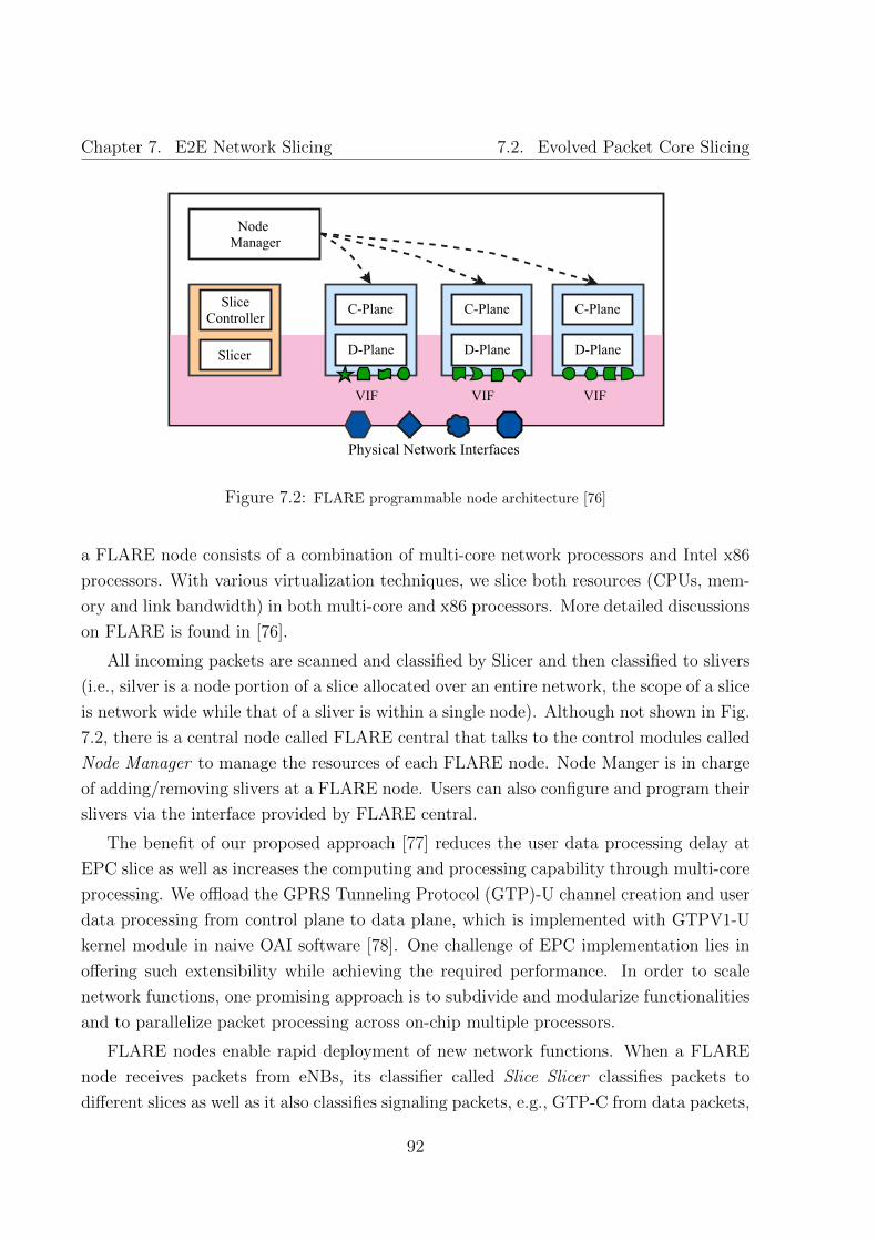
Chapter 7. E2E Network Slicing 7.2. Evolved Packet Core Slicing
Figure 7.2: FLARE programmable node architecture [76]
a FLARE node consists of a combination of multi-core network processors and Intel x86
processors. With various virtualization techniques, we slice both resources (CPUs, mem-
ory and link bandwidth) in both multi-core and x86 processors. More detailed discussions
on FLARE is found in [76].
All incoming packets are scanned and classified by Slicer and then classified to slivers
(i.e., silver is a node portion of a slice allocated over an entire network, the scope of a slice
is network wide while that of a sliver is within a single node). Although not shown in Fig.
7.2, there is a central node called FLARE central that talks to the control modules called
Node Manager to manage the resources of each FLARE node. Node Manger is in charge
of adding/removing slivers at a FLARE node. Users can also configure and program their
slivers via the interface provided by FLARE central.
The benefit of our proposed approach [77] reduces the user data processing delay at
EPC slice as well as increases the computing and processing capability through multi-core
processing. We offload the GPRS Tunneling Protocol (GTP)-U channel creation and user
data processing from control plane to data plane, which is implemented with GTPV1-U
kernel module in naive OAI software [78]. One challenge of EPC implementation lies in
offering such extensibility while achieving the required performance. In order to scale
network functions, one promising approach is to subdivide and modularize functionalities
and to parallelize packet processing across on-chip multiple processors.
FLARE nodes enable rapid deployment of new network functions. When a FLARE
node receives packets from eNBs, its classifier called Slice Slicer classifies packets to
different slices as well as it also classifies signaling packets, e.g., GTP-C from data packets,
92

Chapter 7. E2E Network Slicing 7.2. Evolved Packet Core Slicing
Figure 7.3: EPC Slicing on FLARE Switch [77]
e.g., GTP-U. The signaling packets are then forwarded to control plane while the data
packets are processed in data plane with multi-core processors.
We run the signaling entities of an EPC slice, e.g., MME and the control plane of SP-
GW, in a Docker instance. We can also run HSS entity in another Docker instance within
the same FLARE sliver. These two docker instances are isolated and replaceable without
interfering with one another. For example, we can install different versions of packages
in MME and Home Subscribe Server (HSS) instances even if they may conflict with each
other when installed on the same host machine. The interfaces between EPC and HSS
entities are implemented with internal Ethernet links, such that they communicate with
each other via Transmission Control Protocol (TCP) and Stream Control Transmission
Protocol (SCTP).
The Southbound API is defined between the data plane and control plane so that a
GTP-U tunnel from data plane to the eNB can be established when parsing and processing
GTP-C packets in control plane. When receiving GTP-C packets, MME asks SP-GW to
establish, update and maintain the GTP-U tunnels in data plane. It is also responsible
for transferring GTP tunneling parameters including endpoint identifiers with the Tunnel
Endpoint Identifiers (TEIDs) to eNBs.
In implementing the prototype, we follow OpenFlow’s convention for programming
abstraction. We define our own programming abstraction as Application Programming
93

Chapter 7. E2E Network Slicing 7.3. Radio Access Network Slicing
Interface (API) as follows
< UEID,TEID >< Action >< Stat >, (7.1)
where UEID may be a UE’s IP address assigned by MME through the signaling channel
and Action may be actions such as create/update/remove a GTP-U tunnel. Once the
EPC slicing is in place, the next step is to move on slicing the radio part of the network
as explained in the following section.
7.3 Radio Access Network Slicing
Leveraging the SDN concept, each network slice can be tailored to a particular com-
munication service in such a way that the control plane and data plane are configured
according to different QoS requirements, while defining an open interface between them.
In this section, we focus our discussions on radio access network slicing, where the most
relevant operations that could be tailored to a particular network slice include mobile
association, access control, load balancing and resource scheduling. In order to achieve
those functionalities, the authors in [79] present different kinds of control/data planes
configurations in a network slice with their corresponding cost of implementation and
flexibility comparisons; i) common control plane across slices and dedicated data plane
for each of the slices, ii) dedicated control/user planes and iii) common control plane
and dedicated control/data planes for each slice. Choosing which configuration to mainly
consider depends on the tradeoff between flexibility and cost of implementation.
Once we separate the control and data planes of the RAN, a virtualization technique
is employed to create the virtual instances of the considered RAN resources. Depending
on the selected control/data plane configurations, each virtual RAN instance contains a
dedicated data plane and a common control plane or a dedicated control/data plane or a
common control plane with dedicated control/data plane. The amount of RAN resources
allocated per network slice depends on the QoS requirements, e.g., as defined in Table
7.1), the amount of traffic load, the wireless link quality, etc. Moreover, in presence of
multiple radio access technologies, it is also possible to allocate a RAN resource to a
network slice from a single or multiple RATs. In order to improve flexibility, depending
on the network traffic load, for example to dynamically turn on/off a particular RAT in
a slice reduces the energy consumption of a network slice.
Considering a 4G LTE protocol stack, control and data planes of the Uu (between UE
and eNB) and S1-interfaces (between eNB and EPC) can be separated to provide slice-
94

Chapter 7. E2E Network Slicing 7.3. Radio Access Network Slicing
specific configuration. In the Uu-interface, the UP consists of the packet data convergence
protocol (PDCP), radio link control (RLC) and MAC layers in the protocol stack whereas
the control plane in addition to PDCP, RLC and MAC layers it also includes the radio
resource controller (RRC). However, the main focus of this analysis is on RAN slicing,
i.e. at the air-interface, as we describe it in the following section.
7.3.1 OpenAirInterface based RAN Slicing
In order to emulate RAN slicing at the Uu-interface, we consider an OAI [78] soft-
ware/hardware testbed on top of an LTE technology. Fig.5 depicts the protocol stack
of the OAI soft UE, soft eNB and soft EPC. The ExpressMIMO2 board [78] is used
for real time experimentation and validation of the communication between UEs and
eNBs. Instead of ExpressMIMO2 UEs, commercial-off-the-shelf (COTS) UEs such as
smartphones and LTE dongles can also be used. Intel x86-based PC with Linux oper-
ating system installed are used to emulate the EPC as shown in Fig. 7.5 based on the
discussions presented in Section 7.2.
Figure 7.4: OAI LTE protocol stack and ExpressMIMO2 hardware [78]
Based on the experimentation platform defined in Fig. 7.4, we propose a dynamic
radio resource slicing, also known as dynamic spectrum-level slicing (DSLS) [80], technique
using a single eNB and a single EPC. The prototype system model is shown in Fig. 7.5
where we use a single ExpressMIMO2 board to emulate eNB (i.e. Virtual eNB (VeNB)
instances are created by partitioning the radio resources an eNB into multiple parts each
belonging to each of the VeNB instances), 2 COTS UEs and one Intel-based PC to run the
EPC. The DSLS algorithm dynamically partitions the radio resources of the eNB into two
95

Chapter 7. E2E Network Slicing 7.3. Radio Access Network Slicing
portions each serving VeNB1 and VeNB2 respectively. The detailed problem formulation
and algorithm implementation of the DSLS can be referred in [80].
Figure 7.5: OAI based prototype to implement RAN radio resource slicing [81]
Since the current version of OAI soft eNB only supports 2 UEs, we model the user
distribution in each VeNB as the amount of traffic load generated by each of the UEs,
UE1 and UE2, as depicted in Fig. 7.5, where the radio resources allocated to VeNB1 and
VeNB2 serve UE1 and UE2 respectively.
The configuration of the whole system is divided into two stages: i) installation and
configuration of the OAI eNB, EPC and HSS on a single or different hosts (in our case
in different hosts). At the end of this stage, eNB should be able connect to the EPC
and HSS, ii) configuration of the UE (it includes subscriber identity module-subscriber
identification module (SIM) card configuration) and registration to HSS database, the UE
should be able to attach and connect to eNB.
7.3.2 OAI based Experimentation Results
We implemented the prototype RAN spectrum-level slicer given in Fig. 7.5 with a min-
imal system elements as shown in Fig. 7.6. Based on the system model given in Part
III Chapter 6 Fig. 6.2, we considered two virtual networks (i.e., VN1 and VN2) for
the prototype implementation. We also considered two different traffic models for the
corresponsing VNs: i) icmp packets of packet size 128 Bytes are transmitted in VN1 and
ii) in VN2 the traffic is assumed to follow Poisson distribution with a predefined inten-
sity λ. Moreover, the most interesting functionality is that we defined a resource sharing
agreement among the two VNs. In case of a virtual netwok overload, resource sharing is
enabled only from VN2 to VN1.
We used one Linux based PC in order to emulate both the eNB and UE, in this
experimentation no S1-interface is considered. Since with our considered minimal setting
we can only support one UE in one machine, we created the second UE that belongs
96

Chapter 7. E2E Network Slicing 7.3. Radio Access Network Slicing
Figure 7.6: OAI based minimal prototype to implement DSLS [80] algorithm
Figure 7.7: Radio resource allocation where there is no overload in any of the VNs
to VN2 as a dummy UE where the traffic generated in VN2 is also simulated based on
Poisson distribution. Where as the UE in VN1 is emulated by the Linux based PC as
shown in Fig. 7.6 accepting downlink icmp packets that are sent from OAI eNB. From
Fig. 7.6 the corresponding IP addresses of the virtual ethernet interfaces that emulate the
link (i.e., air-interface) between the eNB and UE is given by oai0 and oai1 respectively
with their corresponding IP address configurations as indicated.
Every TTI the network traffic load is assumed to change in both VNs. In VN1,
we send 6 icmp packets of size 128 Bytes and packet data pattern 2B in hexadecimal
representation every 1ms given by the following command: #ping 10.0.1.2 -s 128
-i 0.001 -l 6 -p 2B . Fig. 7.7 shows the radio resource allocation at the initial state
of the experimentation. Considering 5MHz system bandwidth, the total number of RBs
97

Chapter 7. E2E Network Slicing 7.3. Radio Access Network Slicing
Figure 7.8: Radio resource allocation when VN1 is congested
0 50 100 150 200 250 300Transmission Time Interval (TTI) in msec
0.0
0.5
1.0
1.5
2.0
Trig
ger E
vent
Figure 7.9: The number of trigger events sent to DSLS over the experimentation time duration
available is 25 (BW = 25 - green bar). Where 13 RBs were assigned for VN1 and 12 RBs
for VN2 as indicated in the bar plot by VN1 and VN2 respectively. RQ VN1 represents
the amount of RBs required by VN1 to satisfy its users information transmission, AV VN2
is the amount of RBs available for sharing in VN2 and SH VN1 is the RBs shared to VN1
from VN2 in case of overload based on the predefined network sharing agreement.
Once we start transmission of the icmp packets in the downlink in VN1, the distribution
of the radio resources changes as depicted in Fig. 7.8 where VN1 is overloaded. The red
98

Chapter 7. E2E Network Slicing 7.4. Summary
bar represents the amount of shared RBs to VN1 showing the amount of RBs allocated
could not able to support all the downlink transmissions. In other words, this amount of
shared radio resources enable us to handle more traffic in VN1 resulting in lower packet
dropping rate as compared to the static spectrum-level slicing technique as disscussed in
Part III Chapter 6.
The number of trigger events generated by the Slice Manger and sent to dynamic
spectrum-level slicer, as discussed in details in Part III Chapter 6 Section 6.3, is also
shown in Fig. 7.9. Tracking these trigger events enables us to accurately determine the
inter-arrival time between each of the trigger events tailored to the type of services that
we provide. Moreover, this parameter gives a very important insight to determine if it
is possible to implement this kinds of operations (e.g., DSLS) far from the radio access
points that enables us to take advantage of the global view of a network resulting in a
better optimized network.
7.4 Summary
We believe the two most significant features of network slicing are resource isolation and
programmability on resources that are essential for accommodating individual software
defined network functions and application services within each slice without interfering
with the other functions and services on the coexisting slices. We have just begun extend-
ing the concept of network slicing to 5G mobile networking to accommodate applications
with very different requirements, such as eMBB, mMTC and uMTC, to avoid interference
among those, to guarantee the end-to-end quality of applications. The testbed implemen-
tations will let us to better understand the real challenges for acheiving those goals. We
strongly believe we benefit from network slicing in realizing 5G mobile networking and
beyond. In the following chapters, we discuss the future work and then conclude this
dissertation.
99

Chapter 7. E2E Network Slicing 7.4. Summary
100

Part IV
Future Work and Conclusions


Chapter 8
Future Work
Future developments mainly will be focus on the experimental implementation and eval-
uation of an end-to-end network slicing based on the prototype testbed we presented in
Part III Chapter 7. Where we inject different types of network traffic through real mo-
bile devices accessing different services in order to accurately determine the inter-arrival
times between optimization trigger event occurrences for radio resource sharing specific
to the type of services that we are providing. In addition, we verify the results collected
from the testbed implementation by providing analytical analysis via a more realistic
user traffic model. We will also investigate the scalability issues of our proposed spectrum
slicing approach in relation to an increase in the number of virtual networks with more
complex resource sharing aggreement in the system. Furthermore, we will analyze the
computational capabilities of the Linux based PC that implements the evolved packet
core in our proposed prototype testbed and we investigate how its CPU preformance will
be affected in the coexistence of more virtual networks in the system.
103

Chapter 8. Future Work
104
Chapter 9
Conclusions
In this research dissertation we provided a detailed review of the state-of-the-art on dif-
ferent ways of mitigating inter-cell interference and the technologies that enable wireless
resource virtualization in mobile networks by pointing out the limitations and the improve-
ment opportunities followed by a comprehensive proposed solutions that we discussed in
Parts II and III.
In Part II Chapter 4, we proposed a software-defined framework for mitigating
interference in mobile radio networks. Using the global view of the network, a centralized
interference analysis facilitates an optimized radio resource allocation via abstracting
mobile network system parameters, <time, frequency, space, transmit-power, modulation,
coding, antenna-port>, improving the programmability of the considered network. We
characterized the interference between different communication links (i.e., transmitter-
receiver pairs) in the network via an interference graph, which is computed in a centralized
SDN controller based on the channel information collected with a final goal of providing an
optimization tool for efficient resource scheduling and transmit power allocation. In Part
II Chapter 5 we proposed two spatial scheduling techniques based on the fractional
frequency reuse scheme, to mitigate the inter-cell interference in virtualized small cell
networks. Each approach consists of two schedulers operating over different time scales,
short and long. Depending on the traffic load in the small cells, the spatial scheduler (i.e.,
operating in longer time scale) dynamically changes the antenna beamwidth to partition
the cell area in different sectors every LTE radio frame. One the other hand, the MAC
scheduler operates over a shorter time scale every TTI. Furthermore, we tackled the
problem of modeling the cell coverage using stochastic geometry. Numerical results have
demonstrated our proposed approaches outperform the state-of-the-art solutions over the
same network conditions. Our approaches can also be applied taking into consideration
105

Chapter 9. Conclusions
the changes expected in the physical layer technology for 5G networks and beyond.
In Part III Chapter 6, we proposed a dynamic spectrum-level slicing technique for
HetNets for dynamically allocating radio resources to virtual networks from a centralized
virtual radio resource pool. Numerical results have shown the proposed technique out-
performs the static spectrum-level slicing by reducing the number of dropped packets. In
addition, this technique is not limited to LTE; it can also be applied to different radio
access technologies. Furthermore, we investigated how often the optimization operation
should have to be performed in relation to the achievable network preformance and the
feasibility of implementing the dynamic resource sharing functionality far from the phys-
ical access points (i.e., in a centralized way). Following the discussions on radio resource
slicing, in Part III Chapter 7, we extended the concept of network slicing to 5G mo-
bile networking to accommodate applications with very different requirements, such as
eMBB, mMTC and URLLC, to avoid interference among those, to guarantee the end-to-
end quality of services. Moreover, based on our preliminary work on radio resource slicing,
we presented a test-bed implementation of dynamic spectrum-level slicing technique using
an open-source software/hardware platform, OpenAirInterface.
106

Bibliography
[1] Cisco and/or its affiliates. Cisco Visual Networking Index: Global Mobile Data Traffic
Forecast Update, 2015–2020. Technical report, Feb. 3 2016.
[2] NTT DOCOMO, INC. 5G Radio Access: Requirements, Concept and Technologies.
White paper, NTT, DOCOMO, July 2014.
[3] Q. (Clara) Li, H. Niu, A. (Tolis) Papathanassiou, and G. Wu. 5G Network Capacity
Key Elements and Technologies. IEEE Vehicular Technology Magazine, pages 71–78,
Jan. 31 2014.
[4] J. G. Andrews, S. Buzzi, W. Choi, S. V. Hanly, A. Lozano, A. C. K. Soong, and J.
C. Zhang. What Will 5G Be? IEEE Journal on Selected Areas in Communications,
32(6):1065–1082, June 2014.
[5] B. A. A. Nunes, M. Mendonca, X.-Nam Nguyen, K. Obraczka and T. Turletti. A
Survey of Software-Defined Networking: Past, Present, and Future of Programmable
Networks. IEEE Communications Surveys and Tutorials, 16(3):1617–1634, Jan. 5-19
2014.
[6] T. Shimojo, Y. Takano, A. Khan, S. Kaptchouang, M. Tamura and S. Iwashina.
Future Mobile Core Network for Efficient Service Operation. in Proc. of the first
IEEE Network Softwarization (NetSoft), London, UK, pages 1–6, Apr. 13-17 2015.
[7] A. A. Gebremariam, L. Goratti, R. Riggio, D. Siracusa, T. Rasheed, F. Granelli. A
framework for interference control in Software-Defined mobile radio networks. 12th
Annual IEEE Consumer Communications and Networking Conference (CCNC), Las
Vegas, NV, USA, pages 892–897, Jan. 9-12 2015.
[8] A. A. Gebremariam, T. Bao, D. Siracusa, T. Rasheed, F. Granelli and L. Goratti.
Dynamic Strict Fractional Frequency Reuse for Software-Defined 5G Networks. IEEE
ICC2016, Kuala Lumpur, Malaysia, May 22-27 2016.
107

Bibliography Bibliography
[9] FUJITSU NETWORK COMMUNICATIONS INC. The Benefits of Cloud-RAN
Architecture in Mobile Network Expansion. Technical report, 2801 Telecom Parkway,
Richardson, Texas 75082-3515, Oct. 20 2016.
[10] 5G PPP Architecture Working Group. View on 5g architecture, Jul. 2016.
[11] A deliverable by NGMN Alliance. NGMN 5G White Paper, Feb. 17 2015.
[12] S. Eddine, M. Boldi, O. Bulakci, P. Spapis, M. Schellmann, P. Marsch, M. Saily, J.
F. Monserrat, T. Rosowski, G. Zimmermann, I. D. Silva, M. Tesanovic, M. Shariat
and A. M. Ibrahim. Preliminary Views and Initial Considerations on 5G RAN Ar-
chitecture and Functional Design. Technical report, METIS-II and 5G PPP White
Paper, Mar. 8 2016.
[13] A. A. Gebremariam, M. Chowdhury, A. Goldsmith and F. Granelli. Resource Pooling
via Dynamic Spectrum-level Slicing across Heterogeneous Networks. IEEE CCNC17,
Las Vegas, USA, pages 1–6, Jan. 8-11 2017.
[14] EURECOM. http://www.openairinterface.org/, Last checked Oct. 20, 2016.
[15] A. Nakao, P. Du, Y. Kiriha, F. Granelli, A. A. Gebremariam, T. Taleb and M.
Bagaa. End-to-End Network Slicing for 5G Mobile Networks. Journal of Information
Processing, Information Processing Society of Japan, 25(1):1–10, Jan. 2017.
[16] N. McKeown, T. Anderson, H.Balakrishnan, G. Parulkar, L. Peterson, J. Rexford,
S.Shenker, and J. Turner. OpenFlow: Enabling Innovation in Campus Networks.
ACM SIGCOMM Computer Communication Review, New York, USA, 38(2):69–74,
April 2008.
[17] H. Kim and N.Feamster. Improving Network Management with Improving Network
Management with Software Defined Networking. IEEE Communications Magazine,
pages 114–119, February 2013.
[18] N. Gude, B. Pfaff, T. Koponen, M. Casado, S. Shenker, J. Pettit and N. McKeown.
NOX: Towards an Operating System for Networks. ACM SIGCOMM Computer
Communication Review, 38(3):105–110, July 2008.
[19] A. Gudipati, D. Perry, L. E. Li, and S. Katti. SoftRAN: Software Defined Radio
Access Network. HotSDN’13, Hong Kong, China, pages 25–30, August 16 2013.
108

Bibliography Bibliography
[20] K.-K. Yap, R. Sherwood, M. Kobayashi, T.-Y. Huang, M. Chan, N. Handigol, N.
McKeown, and G. Parulkar. Blueprint for Introducing Innovation into Wireless Mo-
bile Networks. VISA 2010, New Delhi, India, pages 1–8, September 3 2010.
[21] M. Bansal, J. Mehlman, S. Katti and P. Levis. OpenRadio: A Programmable Wireless
Dataplane. HotSDN’12, Helsinki, Finland, pages 109–114, August 2012.
[22] X. Jin, L. E. Li, L. Vanbever and J. Rexford. SoftCell: Scalable and Flexible Cellular
Core Network Architecture. CoNEXT’13, Santa Barbara, California, USA, pages 1–
13, December 9-12 2013.
[23] R. Riggio, K. Gomez, L. Goratti, R. Fedrizzi and T. Rasheed. V–Cell: Going Be-
yond the Cell Abstraction in 5G Mobile Networks. SDNMO workshop in Network
Operations and Management Symposium (NOMS), 2014 IEEE, pages 1–5, 2014.
[24] F. Afroz, K. Sandrasegaran, and H. A. Kim. Interfernce Management in LTE Down-
link Networks. International Journal of Wireless and Mobile Networks (IJWMN),
7(1):91–106, Feb. 2015.
[25] G. Boudreau, J. Panicker, N. Guo, R. Chang, N. Wang and S. Virzic. Interference
Coordination and Cancellation for 4G Networks. IEEE Communications Magazine,
47(4):74–81, Apr. 2009.
[26] A. S. Hamza, S. S. Khalifa, H. S. Hamza and K. Elsayed. A Survey on Inter-Cell
Interference Coordination Techniques in OFDMA-Based Cellular Networks. IEEE
COMMUNICATIONS SURVEYS & TUTORIALS, 15(4):1642–1670, Aug. 13 2013.
[27] N. Saquib, E. Hossain, and D. in Kim. Fractional Frequency Reuse for Interfer-
ence Management in LTE-Advanced HetNets. IEEE Wireless Communications,
20(2):113–122, Apr. 25 2013.
[28] Siemens R1-050738. Interference mitigation - Considerations and Results on Fre-
quency Reuse. RAN WG, London, UK, 1(42), Aug./Sep. 2005.
[29] X. Fan, Chen Si and X. Zhang. An Inter-Cell Interference Coordination Technique
Based on Users’ Ratio and Multi-Level Frequency Allocations. International Confer-
ence on Wireless Communications, Networking and Mobile Computing, pages 788–
802, Sep. 2007.
109

Bibliography Bibliography
[30] R. Kokku, R. Mahindra, H. Zhang, and S. Rangarajan. NVS: A substrate for virtual-
izing wireless resources in cellular networks. IEEE/ACM Transaction on Networking,
20(5):1333–1346, Oct. 2012.
[31] C. Liang and F. Richard Yu. Wireless Network Virtualization: A Survey, Some
Research Issues and Challenges. IEEE Communication Surveys and Tutorials,
17(1):358–380, Jan. 21 2014.
[32] X. Costa-Perez, J. Swetina, G. Tao, R. Mahindra, and S. Rangarajan. Radio access
network virtualization for future mobile carrier networks. IEEE Communication
Magazine, 51(7):22–35, July 2013.
[33] K. Pentikousis, W. Yan and H. Weihua. Mobileflow: Toward software-defined mobile
networks. IEEE Communication Magazine, 51(7):44–53, Jul. 2013.
[34] Y. Zaki. LTE Optimization and Mobile Network Virtualization. Springer, 2012.
[35] Y. Zaki, L. Zhao, C. Goerg, and A. Timm-Giel. LTE mobile network virtualization.
Mobile Net. & Applications, 16(4):424–432, Aug. 2011.
[36] Y. Zaki, Z. Liang, C. Goerg, and A. Timm-Giel. LTE wireless virtualization and
spectrum management. in Proc. 3rd Joint IFIP WMNC, Budapest, Hungary, pages
1–6, Oct. 2010.
[37] M. Yang, Y. Li, D. Jin, L. Su, S. Ma and L. Zeng. OpenRAN: A Software-defined
RAN Architecture via Virtualization. in Proc. ACM SIGCOMM, Hong Kong, China,
pages 549–550, Aug. 12-16 2013.
[38] J. Kempf, B. Johansson, S. Pettersson, H. Luning, and T. Nilsson. Moving the
mobile evolved packet core to the cloud. in Proc. IEEE Int’l Conf. Wireless & Mobile
Computing, Networking and Communication (WiMob), Barcelona, Spain, Oct. 2012.
[39] L. E. Li, Z. M. Mao, and J. Rexford. Cellsdn: Software-defined Cellulare networks.
Princeton University Computer Science, Technical Report, 2012.
[40] V. Philip, Y. Gourhant, and D. Zeghlache. OpenFlow as an Architecture for e-
Node B Virtualization. ser. Lecture Notes of the Institure for Computer Sciences,
Social Informatics and Telecommunications Engineering, Springer Berlin Heidelberg,
92(5):49–63, 2012.
110
Bibliography Bibliography
[41] R. Sherwood, G. Gibb, K.-K. Yap, G. Appenzeller, M. Casado, N. McKeown
and G. Parulkar. FlowVisor:A Network Virtualization Layer. Technical Report
OPENFLOW-TR-2009-1, Deutsche Telekom Inc. Stanford University, Nicira Net-
works, October 14 2009.
[42] L. Caeiro, F. D. Cardoso, and L. M. Correia. Adaptive Allocation of Virtual Ra-
dio Resources over Heterogeneous Wireless Networks. European Wireless, Poznan,
Poland, pages 1–7, Apr. 18-20 2012.
[43] K. Nakauchi, K. Ishizu, H. Murakami, A. Nakoa and H. Harada. AMPHIBIA: A
Cognitive Virtualization Platform for End-to-End Slicing. in Proc. IEEE Int. Conf.
Commun. (ICC), June 5-9 2011.
[44] P. Cadieri. Modeling Interference in Wireless Ad Hoc Networks. IEEE Communica-
tions Surveys and Tutorials, 12(4):551–572, 2010.
[45] Wireless Technologies/Signal generators. Continuing in the direction of LTE-
Advanced: the latest test signals for LTE Rel. 9 White Paper. Rode and Schwarz.
[46] K. Jain, J. Padhye, V. Padmanabhan and L. Qiu. Impact of Interference on Multi-
hop Wireless Network Performance. MobiCom’03, San Diego, California, USA, pages
1–14, September 14-19 2003.
[47] D. L.-Perez, A. Ladanyi, A. Juttner, H. Rivano and J. Zhang. Optimization Method
for the Joint Allocation of Modulation Schemes, Coding Rates, Resource Blocks
and Power in Self-Organizing LTE Networks. Mini-Conference at INFOCOM, 2011
Proceedings IEEE, Shanghai, Chaina, pages 111–115, April 10-15 2011.
[48] A. Gupta, and R. K. Jha. A Survey of 5G Network: Architecture and Emerging
Technologies. IEEE Access, 3:1206–1232, July 28 2015.
[49] N. Bhushan, J. Li, D. Malladi, R. Gilmore, D. Brenner, A. Damnjanovic, R. T.
Sukhavasi, C. Patel, and S. Geirhoferx. Network Densification: The Dominant Theme
for Wireless Evolution into 5G. IEEE Communications Magazine, 52(2):82–89, Feb.
2014.
[50] R. Cohen, and G. Grebla. Joint Scheduling and Fast Cell Selection in OFDMA
Wireless Networks. Networking, IEEE/ACM Transactions, 23(1):114–125, Feb. 2015.
111

Bibliography Bibliography
[51] J. Umehara, Y. Kishiyama, and K. Higuchi. Enhancing User Fairness in Non-
orthogonal Access with Successive Interference Cancellation for Cellular Downlink.
Proceedings of the 2012 IEEE ICCS, pages 324–328, 2012.
[52] A. Daeinabi, K. Sandrasegaran, and X. Zhu. Survey of Intercell Interference Mit-
igation Techniques in LTE Downlink Networks. Telecommunication Networks and
Applications Conference (ATNAC), Australasian, Brisbane, QLD, (1-6), Nov. 7-9
2012.
[53] R. Kwan, and C. Leung. A Survey of Scheduling and Interference Mitigation in LTE.
Journal of Electrical and Computer Engineering-Special issue on LTE/LTE-advanced
cellular communication networks, 2010(1):1–10, Jan. 2010.
[54] T. Novlan, J. G. Andrews, I. Sohn, R. K. Ganti, and A. Ghosh. Comparison of
Fractional Frequency Reuse Approaches in the OFDMA Cellular Downlink. IEEE
Global Telecommunications Conference(GLOBECOM), Miami, FL, pages 1–5, 2010.
[55] R. Y. Chang, Z. Tao, J. Zhang, and C.-C. J. Kuo. A Graph Approach to Dynamic
Fractional Frequency Reuse (FFR) in Multi-Cell OFDMA Networks. IEEE Inter-
national Conference on Communications, Dresden, Germany, pages 1–6, June 14-18
2009.
[56] F. Bendaoud, M. Abdennebi and F. Didi. Survey On Scheduling And Radio Resources
Allocation In Lte. International Journal of Next-Generation Networks (IJNGN),
6(1):17–29, March 2014.
[57] M. Bansal and V. Venkaiah. Improved Fully Polynomial time Approximation Scheme
for the 0-1 Multiple-choice Knapsack Prolem. SIAM Conference on Discrete Mathe-
matics, pages 1–10, 2004.
[58] R. Cohen, L. Katzir, and D. Raz. An efficient approximation for the Generalized
Assignment Problem. Information Processing Letters, 100(4):162–166, Nov. 30 2006.
[59] Fujitsu Network Communications, Inc. GX4000 E-Band Radio. 7.0:1–4, August
2014.
[60] H. Raza. A brief survey of radio access network backhaul evolution: part I. Com-
munications Magazine, IEEE, 49(6):164–171, 2011.
112

Bibliography Bibliography
[61] A. A. Gebremariam, T. Bao, D. Siracusa, T. Rasheed, F. Granelli and L. Goratti.
Dynamic Strict Fractional Frequency Reuse for Software-Defined 5G Networks. IEEE
ICC, Kuala Lumpur, Malaysia, pages 1–6, May 22-27 2016.
[62] T. D. Novlan, R. K. Ganti, A. Ghosh, and J. G. Andrews. Analytical Evaluation of
Fractional Frequency Reuse for OFDMA Cellular Networks. IEEE Transactions on
Wireless Communications, 10(12):4294–4305, Dec. 2011.
[63] J. G. Andrews, F. Baccelli, and R. K. Ganti. A Tractable Approach to Coverage and
Rate in Cellular Networks. IEEE Transactions on Communications, 59(11):3122–
3134, Nov. 2011.
[64] M. Haenggi, and R. K. Ganti. Interference in Large Wireless Networks, volume 3.
now Publishers Inc., Hanover, MA, USA, and AD Delft, The Netherlands, 2009.
[65] M. Haenggi, J. G. Andrews, F. Baccelli, O. Dousse, and M. Franceschetti. Stochastic
Geometry and Random Graphs for the Analysis and Design of Wireless Networks.
IEEE Journal on Selected Areas in Communications, 27(7):1029–1046, Sept. 2009.
[66] K. –K. Yap, Rob Sherwood, M. Kobayashi, T. -Y. Huang, M. Chan, N. Handigol, N.
McKeown and G. Parulkar. Blueprint for introducing innovation into wireless mobile
networks. in Proc. of VISA’10, pages 1–8, 2010.
[67] J. Sachs and S. Baucke. Virtual radio: A framework for configurable radio networks.
in Proc. Annu. Int. WICON, Maui, HI, USA, pages 1–7, Nov. 17-19 2008.
[68] A. Gudipati, L. E. Li, S. Katti. Radio Visor: A Slicing Plane for Radio Access
Networks. HotSDN’14, Chicago, IL, USA, pages 237–238, Aug. 22 2014.
[69] M. Kalil, A. Shami, and Y. Ye. Wireless Resources Virtualization in LTE Systems.
IEEE INFOCOM Workshops, Toronto, ON, pages 363–368, Apr. 27-May 2, 2014
2014.
[70] Scipy developers. https://www.scipy.org/citing.html, last checked May 29, 2016.
[71] E-UTRA 3GPP, TSG RAN. Further advancements for E-UTRA physical layer as-
pects (Release 9). Technical report, 3GPP Organization Partners, 2010.
[72] 5G PPP Architecture Working Group, View on 5G Architecture, Jul. 2016.
[73] A deliverable by NGMN Alliance, NGMN 5G White Paper, Feb. 17, 2015.
113

Bibliography Bibliography
[74] F. Granelli, A. A. Gebremariam, M. Usman, F. Cugini, V. Stamati, M. Altiska and
P. Chatzimisios. Software Defined and Virtualized Wireless Acess in Future Wireless
Networks: Scenarios and Standards. IEEE Communication Magazine, pages 26–34,
Jun. 2015.
[75] 5GMF. 5g mobile communications systems for 2020 and beyond. 5GMF White Paper
Version 1.01, Jul. 4 2016.
[76] FLARE. Open deeply programmable network node architecture, 2016.
[77] A. Nakao, P. Du, Y. Kiriha, F. Granelli, A. A. Gebremariam, T. Taleb and M.
Bagaa. End-to-end network slicing for 5g mobile networks. Journal of Information
Processing, 25(1):1–10, Jan. 2017 2017.
[78] N. Nikaein, M. K. Marina, S. Manickam, A. Dawson, R. Knopp and C. Bonnet.
Openairinterface: A flexible platform for 5g research. ACM SIGCOMM, NY, USA,
44(5):33–38, Oct. 2014.
[79] K. Katsalis, N. Nikaein, E. Schiller, R. Favraud and T. I. Braun. 5G Architectural
Design Patterns. IEEE ICC Workshops: 3rd Workshop on 5G Architecture, Kuala
Lumpur, Malaysia, pages 1–6, May 23-27 2016.
[80] A. A. Gebremariam, M.Chowdhury, A. Goldsmith and F. Granelli. Resource pooling
via dynamic spectrum-level slicing across heterogeneous networks. IEEE CCNC, Las
Vegas, USA, pages 1–6, Jan. 8-11 2017.
[81] A. A. Gebremariam, M.Chowdhury, A. Goldsmith and F. Granelli. An openairin-
terface based implementation of dynamic spectrum-level slicing across heterogeneous
networks. IEEE CCNC, Las Vegas, USA, pages 1–2, Jan. 8-11 2017.
114