Embed Size (px)
Citation preview

Reading University Seminar
Resonant RossbyWave Triads
and theSwinging Spring
Peter Lynch, Met Eireann, Dublin
Department of Meteorology, University of Reading,
2nd February, 2004.

In a Nutshell
A mathematical equivalence with asimple mechanical system
sheds light on the dynamics ofresonant Rossby waves
in the atmosphere.
2

The Swinging Spring
Two distinctoscillatory modeswith two distinctrestoring forces:
Elastic orspringy modes
Pendular orswingy modes
3

The Swinging Spring
Two distinctoscillatory modeswith two distinctrestoring forces:
Elastic orspringy modes
Pendular orswingy modes
Take a peek at the Java Applet
3

In a paper in 1981, Breitenberger and Muellermade the following comment:
This simple system looks like a toy at best,but its behaviour is astonishingly complex,
with many facets of more than academic lustre.
I hope to convince you of the validity of this remark.
4

Information and Resources
http://www.maths.tcd.ie/∼plynch
Papers on Spring and Triads:Click on ‘Publications’.
Java Applet on Swinging Spring:Click on ‘The Swinging Spring’.
Slides of this talk (Sapporo Version):Click on ‘Talks’.
Matlab Code for Spring and Triads:Click on ‘Rossby Wave Triads’.
5

Bulletin of the AMS, May, 2003
6

Bulletin of the AMS, May, 2003
Printed version for dilettantes and smatterers in mathematics.
Full mathematical details are in the Electronic Supplement.
6

Motivation
The linear normal modes of the atmosphere fall into twocategories, the low frequency Rossby waves and the highfrequency gravity waves.
7

Motivation
The linear normal modes of the atmosphere fall into twocategories, the low frequency Rossby waves and the highfrequency gravity waves.
The Swinging Spring is a simple mechanical system havinglow frequency and high frequency oscillations.
7

Motivation
The linear normal modes of the atmosphere fall into twocategories, the low frequency Rossby waves and the highfrequency gravity waves.
The Swinging Spring is a simple mechanical system havinglow frequency and high frequency oscillations.
The elastic oscillations of the spring are analogues of thehigh frequency gravity waves in the atmosphere.
The low frequency pendular motions correspond to the ro-tational or Rossby-Haurwitz waves.
7

Analogy and Equivalence
Analogies are interesting.Equiavlences are useful.
Value of the Analogy
1. Wave-like motions
2. Initialization
3. Filtered Equations
4. Slow manifold theory
Power of the Equivalence
1. Triad Resonance
2. Rossby Wave Precession
3. Predictability
8

Original Reference
First comprehensive analysis of the elastic pendulum:
Oscillations of an Elastic Pendulum asan Example of the Oscillations of Two
Parametrically Coupled Linear Systems.
Vitt and Gorelik (1933).
Inspired by analogy with Fermi resonance of CO2.
Translation of this paper available as
Historical Note #3 (1999)
Published by Met Eireann.
Available at URL:
http://www.maths.tcd.ie/∼plynch
9

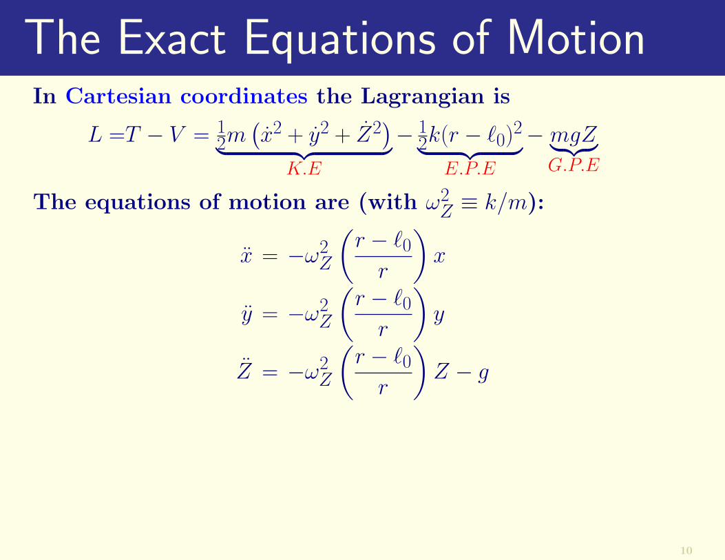
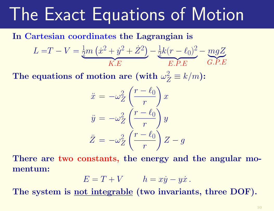
The Exact Equations of MotionIn Cartesian coordinates the Lagrangian is
L =T − V = 12m
(x2 + y2 + Z2
)︸ ︷︷ ︸K.E
− 12k(r − `0)
2︸ ︷︷ ︸E.P.E
− mgZ︸ ︷︷ ︸G.P.E
10
The Exact Equations of MotionIn Cartesian coordinates the Lagrangian is
L =T − V = 12m
(x2 + y2 + Z2
)︸ ︷︷ ︸K.E
− 12k(r − `0)
2︸ ︷︷ ︸E.P.E
− mgZ︸ ︷︷ ︸G.P.E
The equations of motion are (with ω2Z ≡ k/m):
x = −ω2Z
(r − `0r
)x
y = −ω2Z
(r − `0r
)y
Z = −ω2Z
(r − `0r
)Z − g
10
The Exact Equations of MotionIn Cartesian coordinates the Lagrangian is
L =T − V = 12m
(x2 + y2 + Z2
)︸ ︷︷ ︸K.E
− 12k(r − `0)
2︸ ︷︷ ︸E.P.E
− mgZ︸ ︷︷ ︸G.P.E
The equations of motion are (with ω2Z ≡ k/m):
x = −ω2Z
(r − `0r
)x
y = −ω2Z
(r − `0r
)y
Z = −ω2Z
(r − `0r
)Z − g
There are two constants, the energy and the angular mo-mentum:
E = T + V h = xy − yx .
The system is not integrable (two invariants, three DOF).
10

The HamiltonianAt equilibrium, the elastic restoring force is balanced by theweight
k(`− `0) = mg or ` = `0
(1 +
mg
k`0
).
11

The HamiltonianAt equilibrium, the elastic restoring force is balanced by theweight
k(`− `0) = mg or ` = `0
(1 +
mg
k`0
).
For the time being, we consider motion in a plane.
11

The HamiltonianAt equilibrium, the elastic restoring force is balanced by theweight
k(`− `0) = mg or ` = `0
(1 +
mg
k`0
).
For the time being, we consider motion in a plane.
The total energy is sum of kinetic, elastic potential andgravitational potential energy.
Radial Momentum : pr = mr
Angular Momentum : pθ = mr2θ
H =1
2m
(p2r +
p2θ
r2
)+ 1
2k(r − `0)2 −mgr cos θ
11

The Canonical EquationsThe canonical equations of motion are:
θ = pθ/mr2
pθ = −mgr sin θ
r = pr/m
pr = p2θ/mr
3 − k(r − `0) +mg cos θ
12

The Canonical EquationsThe canonical equations of motion are:
θ = pθ/mr2
pθ = −mgr sin θ
r = pr/m
pr = p2θ/mr
3 − k(r − `0) +mg cos θ
These equations may also be written symbolically in vectorform
X + LX + N(X) = 0
The state vector X specifies a point in 4-dimensional phasespace.
12

The Canonical EquationsThe canonical equations of motion are:
θ = pθ/mr2
pθ = −mgr sin θ
r = pr/m
pr = p2θ/mr
3 − k(r − `0) +mg cos θ
These equations may also be written symbolically in vectorform
X + LX + N(X) = 0
The state vector X specifies a point in 4-dimensional phasespace.
If Hamiltonian methods are unfamiliar, the equations may be derived using standard Newtonian dynamics.
12

Linear Normal ModesSuppose that amplitude of motion is small:
d
dt
θpθr′
pr
=
0 1/m`2 0 0
−mg` 0 0 00 0 0 1/m0 0 −k 0
θpθr′
pr
13

Linear Normal ModesSuppose that amplitude of motion is small:
d
dt
θpθr′
pr
=
0 1/m`2 0 0
−mg` 0 0 00 0 0 1/m0 0 −k 0
θpθr′
pr
The matrix is block-diagonal:
X =
(YZ
), Y =
(θpθ
), Z =
(r′
pr .
)Linear dynamics evolve independently:
Y =
(0 1/m`2
−mg` 0
)Y , Z =
(0 1/m−k 0
)Z .
SLOW FAST
13

The motion described by Y is the rotational component:
θ + (g/`)θ = 0
14

The motion described by Y is the rotational component:
θ + (g/`)θ = 0
The motion described by Z is elastic component:
r′ + (k/m)r′ = 0
14

The motion described by Y is the rotational component:
θ + (g/`)θ = 0
The motion described by Z is elastic component:
r′ + (k/m)r′ = 0
Eigenfrequencies, or normal mode frequencies:
ωR =√g/` , ωE =
√k/m
14

The motion described by Y is the rotational component:
θ + (g/`)θ = 0
The motion described by Z is elastic component:
r′ + (k/m)r′ = 0
Eigenfrequencies, or normal mode frequencies:
ωR =√g/` , ωE =
√k/m
Ratio of rotational and elastic frequencies:
ε ≡(ωRωZ
)=
√mg
k`.
14
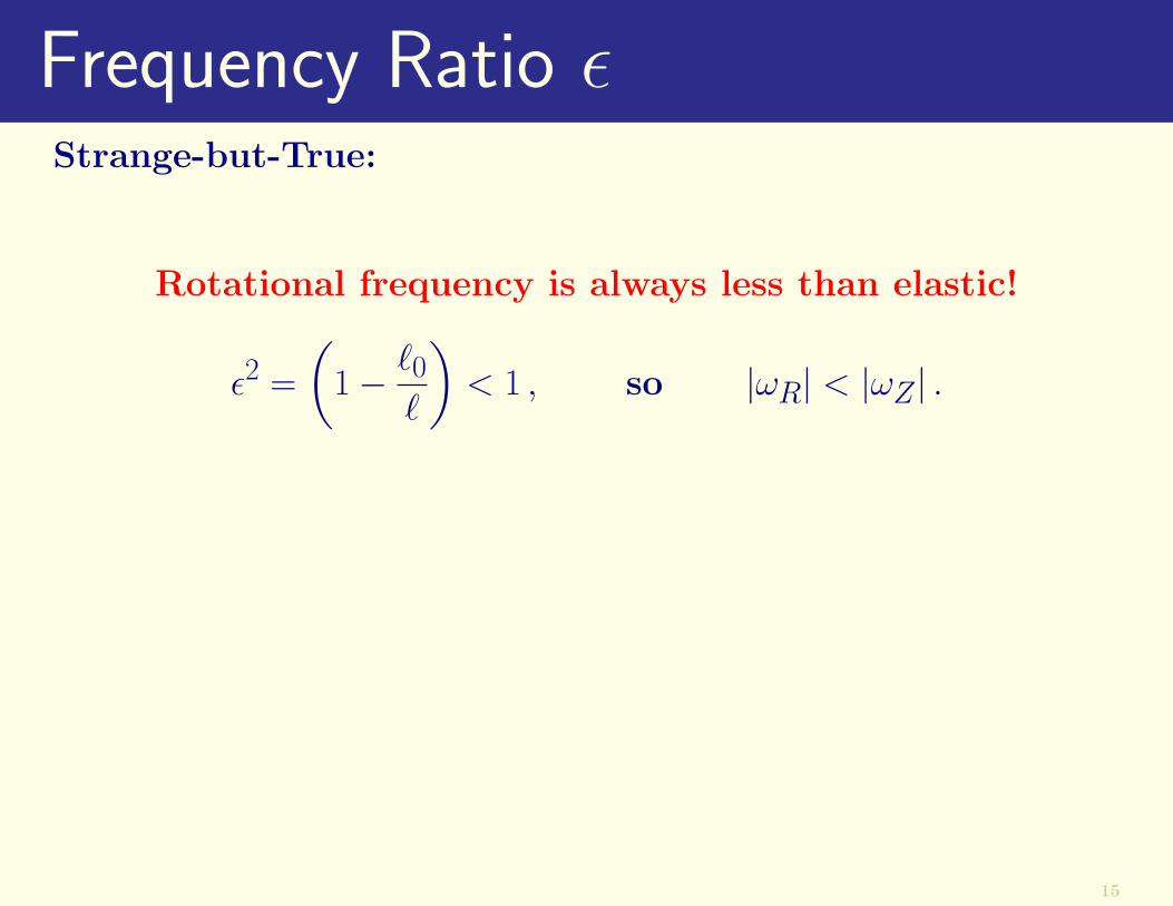
Frequency Ratio εStrange-but-True:
Rotational frequency is always less than elastic!
ε2 =
(1− `0
`
)< 1 , so |ωR| < |ωZ| .
15
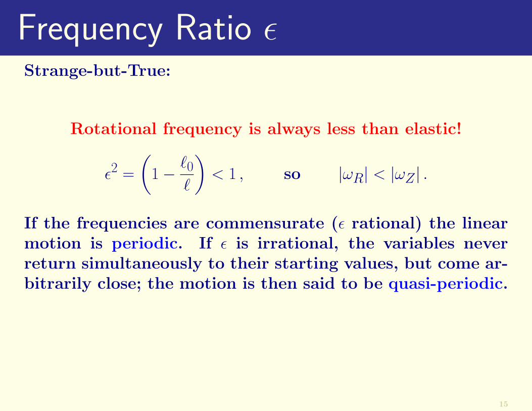
Frequency Ratio εStrange-but-True:
Rotational frequency is always less than elastic!
ε2 =
(1− `0
`
)< 1 , so |ωR| < |ωZ| .
If the frequencies are commensurate (ε rational) the linearmotion is periodic. If ε is irrational, the variables neverreturn simultaneously to their starting values, but come ar-bitrarily close; the motion is then said to be quasi-periodic.
15

Large Frequency Separation: ε 1.KAM Block
We will assume (for the moment) parameters such that:
ε ≡(ωR
ωE
)=
√mg
k` 1 .
Linear normal modes are clearly distinct: the rotationalmode has low frequency (LF) and the elastic mode has highfrequency (HF).
16
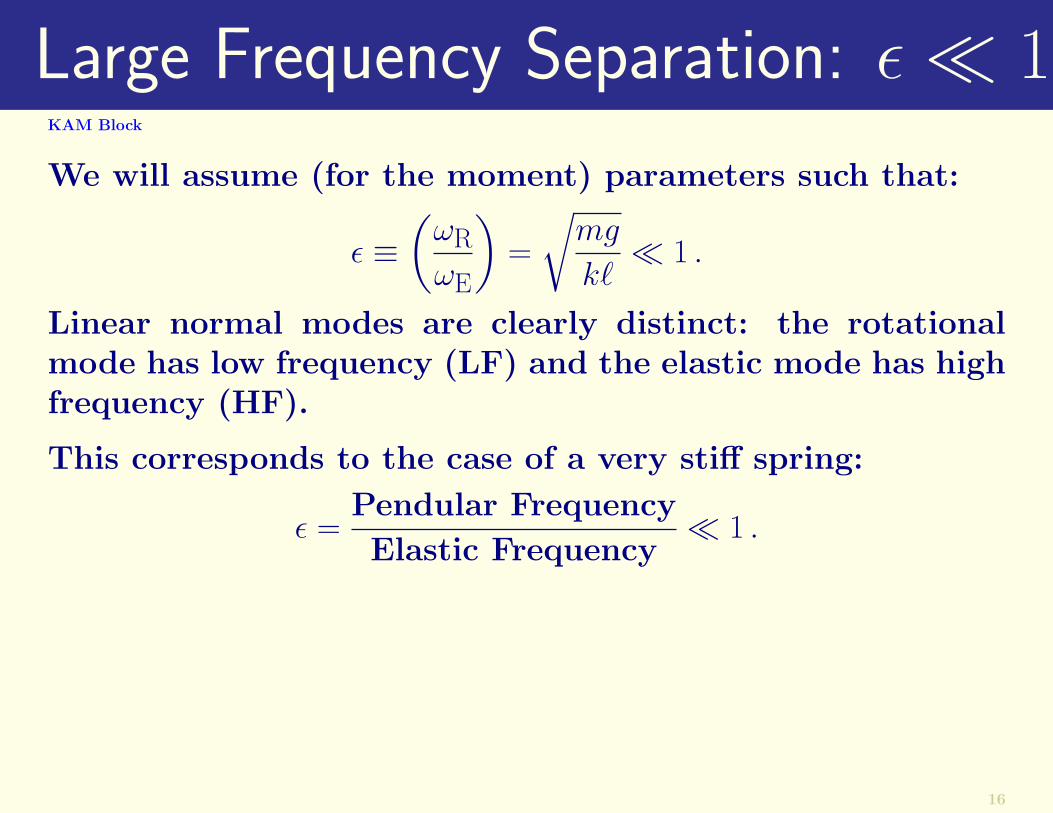
Large Frequency Separation: ε 1.KAM Block
We will assume (for the moment) parameters such that:
ε ≡(ωR
ωE
)=
√mg
k` 1 .
Linear normal modes are clearly distinct: the rotationalmode has low frequency (LF) and the elastic mode has highfrequency (HF).
This corresponds to the case of a very stiff spring:
ε =Pendular Frequency
Elastic Frequency 1 .
Analogy:(Gravity Wave
Frequency
)
(Rossby Wave
Frequency
)16

For ε = 0, there is no coupling between the modes.
For ε 1 the coupling is weak.We can apply classical Hamiltonian perturbation theory.
17

For ε = 0, there is no coupling between the modes.
For ε 1 the coupling is weak.We can apply classical Hamiltonian perturbation theory.
The consequences of the Kolmogorov-Arnol’d-Moser (KAM)Theorem for the swinging spring are discussed in:
Lynch, Peter, 2002: The Swinging Spring:A Simple Model for Atmospheric Balance.At URL:
http://www.maths.tcd.ie/∼plynch
Only a bare outline will be given here.
17

Outline of KAM TheoryI. Completely Integrable Hamiltonian Systems
The key to integrating a Hamiltonian system with n degreesof freedom is to find n independent constants of motion.
18

Outline of KAM TheoryI. Completely Integrable Hamiltonian Systems
The key to integrating a Hamiltonian system with n degreesof freedom is to find n independent constants of motion.
Suppose that we have found n such constants, Ik. We definea canonical transformation to new coordinates, treating Ikas the new momenta, and denoting the new conjugate po-sition coordinates as φk.
Since the Ix’s are constant, the trajectories are confined toan n-dimensional manifold M of the 2n-dimensional phasespace. For bounded motion the manifold M may be shownto have the topology of an n-torus, that is, the cartesianproduct of n circles.
18
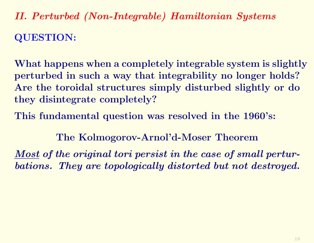
II. Perturbed (Non-Integrable) Hamiltonian Systems
QUESTION:
What happens when a completely integrable system is slightlyperturbed in such a way that integrability no longer holds?Are the toroidal structures simply disturbed slightly or dothey disintegrate completely?
19
II. Perturbed (Non-Integrable) Hamiltonian Systems
QUESTION:
What happens when a completely integrable system is slightlyperturbed in such a way that integrability no longer holds?Are the toroidal structures simply disturbed slightly or dothey disintegrate completely?
This fundamental question was resolved in the 1960’s:
The Kolmogorov-Arnol’d-Moser Theorem
Most of the original tori persist in the case of small pertur-bations. They are topologically distorted but not destroyed.
19

Poincare SectionsTo visualise the motion, we choose a two-dimensional sur-face and plot the intersection of a trajectory each time itpasses through the surface in a particular direction. This iscalled a Poincare section.Two especially convenient choices are
The ‘slow-plane’ (ρ = 0, pρ > 0)
The ‘fast-plane’ (ϑ = 0, pϑ > 0)
20

Poincare SectionsTo visualise the motion, we choose a two-dimensional sur-face and plot the intersection of a trajectory each time itpasses through the surface in a particular direction. This iscalled a Poincare section.Two especially convenient choices are
The ‘slow-plane’ (ρ = 0, pρ > 0)
The ‘fast-plane’ (ϑ = 0, pϑ > 0)
If the motion is integrable, the trajectory lies on a toruswhich cuts the section in a smooth curve.
For non-integrable motion, the system explores a three-dimen-sional region of the energy level, whose intersection with aplane is an area rather than a curve.
20

Poincare Section for total energy E = 1.8. ε = 0.025.
-3
-2
-1
0
1
2
3
-3 -2 -1 0 1 2 3
a
21

Poincare Section for total energy E = 1.8. ε = 0.25.
-3
-2
-1
0
1
2
3
-3 -2 -1 0 1 2 3
g
22

Poincare Section for total energy E = 1.8. ε = 0.40.
-3
-2
-1
0
1
2
3
-3 -2 -1 0 1 2 3
i
23

Regular and Chaotic MotionRegular and Chaotic Motion Block
We wish to discuss the phenomenon of Resonance for thespring, and its Pulsation and Precession.
Resonance occurs for
ε =1
2.
Clearly, this is far from the quasi-integrable case of small ε.
However, for small amplitudes, the motion is also quasi-integrable. We look at two numerical solutions, one withsmall amplitude, one with large.
24

Horizontal plan: Low energy case
25

Horizontal plan: High energy case
26

The Phenomenon of Precession• When started with almost vertical springing motion, themovement gradually develops into an essentially horizontalswinging motion.• This does not persist, but is soon replaced by springyoscillations similar to the initial motion.• Again a horizontal swing develops, but now in a differentdirection.• This variation between springy and swingy motion con-tinues indefinitely.• The change in direction of the swing plane from onehorizontal excursion to the next is difficult to predict:• The plane of swing precesses in a manner which is quitesensitive to the initial conditions.
27

The Phenomenon of Precession• When started with almost vertical springing motion, themovement gradually develops into an essentially horizontalswinging motion.• This does not persist, but is soon replaced by springyoscillations similar to the initial motion.• Again a horizontal swing develops, but now in a differentdirection.• This variation between springy and swingy motion con-tinues indefinitely.• The change in direction of the swing plane from onehorizontal excursion to the next is difficult to predict:• The plane of swing precesses in a manner which is quitesensitive to the initial conditions.
Demo: Precession of Swinging Spring.
or Peek at the Applet.
27

The Resonant CaseThe Lagrangian (to cubic order) is
L = 12
(x2 + y2 + z2
)− 1
2
(ω2R(x2 + y2) + ω2
Zz2)
+ 12λ(x2 + y2)z ,
We study the resonant case:
ωZ = 2ωR .
28

The Resonant CaseThe Lagrangian (to cubic order) is
L = 12
(x2 + y2 + z2
)− 1
2
(ω2R(x2 + y2) + ω2
Zz2)
+ 12λ(x2 + y2)z ,
We study the resonant case:
ωZ = 2ωR .
The equations of motion are
x + ω2Rx = λxz
y + ω2Ry = λyz
x + ω2Zx = 1
2λ(x2 + y2) .
The system is not integrable.
28

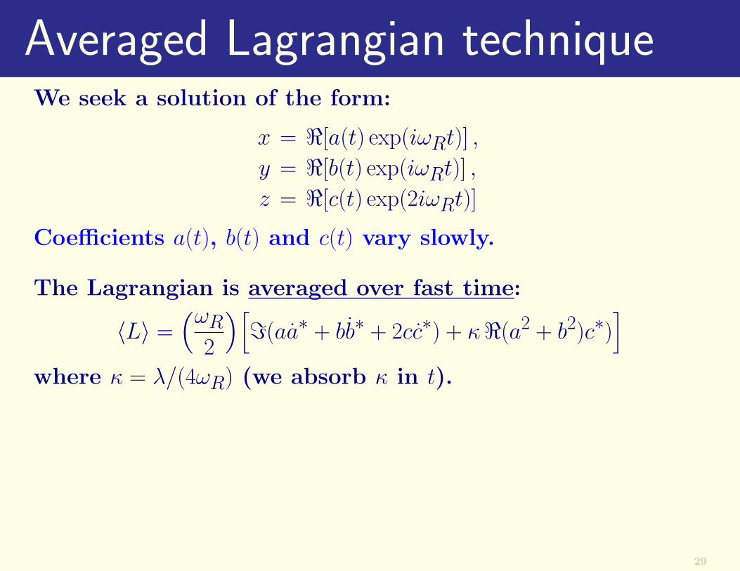
Averaged Lagrangian techniqueWe seek a solution of the form:
x = <[a(t) exp(iωRt)] ,
y = <[b(t) exp(iωRt)] ,
z = <[c(t) exp(2iωRt)]
Coefficients a(t), b(t) and c(t) vary slowly.
29
Averaged Lagrangian techniqueWe seek a solution of the form:
x = <[a(t) exp(iωRt)] ,
y = <[b(t) exp(iωRt)] ,
z = <[c(t) exp(2iωRt)]
Coefficients a(t), b(t) and c(t) vary slowly.
The Lagrangian is averaged over fast time:
〈L〉 =(ωR
2
)[=(aa∗ + bb∗ + 2cc∗) + κ<(a2 + b2)c∗)
]where κ = λ/(4ωR) (we absorb κ in t).
29

Averaged Lagrangian techniqueWe seek a solution of the form:
x = <[a(t) exp(iωRt)] ,
y = <[b(t) exp(iωRt)] ,
z = <[c(t) exp(2iωRt)]
Coefficients a(t), b(t) and c(t) vary slowly.
The Lagrangian is averaged over fast time:
〈L〉 =(ωR
2
)[=(aa∗ + bb∗ + 2cc∗) + κ<(a2 + b2)c∗)
]where κ = λ/(4ωR) (we absorb κ in t).
We then derive the Euler-Lagrange equations resulting fromthis averaged Lagrangian.
29

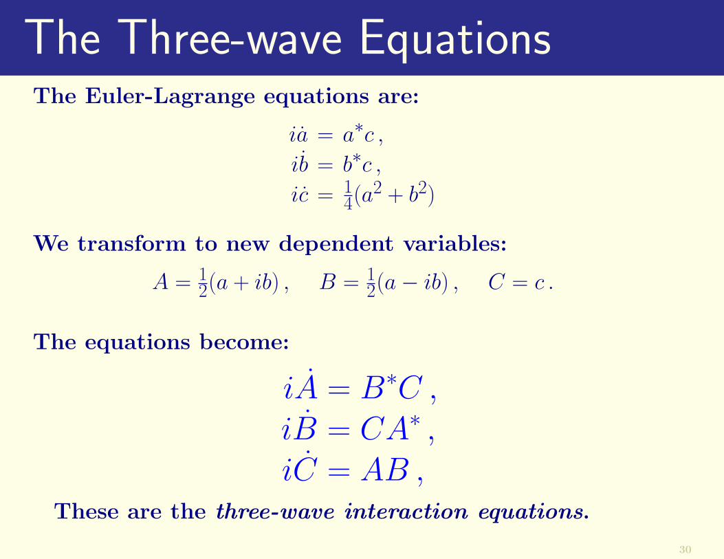
The Three-wave EquationsThe Euler-Lagrange equations are:
ia = a∗c ,ib = b∗c ,ic = 1
4(a2 + b2)
30

The Three-wave EquationsThe Euler-Lagrange equations are:
ia = a∗c ,ib = b∗c ,ic = 1
4(a2 + b2)
We transform to new dependent variables:
A = 12(a + ib) , B = 1
2(a− ib) , C = c .
30
The Three-wave EquationsThe Euler-Lagrange equations are:
ia = a∗c ,ib = b∗c ,ic = 1
4(a2 + b2)
We transform to new dependent variables:
A = 12(a + ib) , B = 1
2(a− ib) , C = c .
The equations become:
iA = B∗C ,iB = CA∗ ,iC = AB ,
These are the three-wave interaction equations.
30

InvariantsThe three-wave equations conserve the following three quan-tities,
H = 12(ABC
∗ + A∗B∗C)
N = |A|2 + |B|2 + 2|C|2
J = |A|2 − |B|2 .The Three-wave equations are completely integrable.
31

InvariantsThe three-wave equations conserve the following three quan-tities,
H = 12(ABC
∗ + A∗B∗C)
N = |A|2 + |B|2 + 2|C|2
J = |A|2 − |B|2 .The Three-wave equations are completely integrable.
Physically significant combinations of N and J:
N+ ≡ 12(N + J) = |A|2 + |C|2 ,
N− ≡ 12(N − J) = |B|2 + |C|2 .
These are the Manley-Rowe relations.H, N+ and N− provide three independent constants of themotion. Constant N+ or N− correspond to orthogonal fam-ilies of circular cylinders in phase-space.
31

Surfaces of Revolution
Motion is on the intersection with plane of constant X.
32

Ubiquity of Three-Wave EquationsModulation equations for wave inter-
actions in fluids and plasmas.
Three-wave equations govern envelopdynamics of light waves in an inhomo-geneous material; and phonons in solids.
Maxwell-Schrodinger envelop equationsfor radiation in a two-level resonantmedium in a microwave cavity.
Euler’s equations for a freely rotatingrigid body (when H = 0).
33

Precession of the Swing PlaneBy transforming to rotating co-ordinates, we can derive anexpression for the slow rotation Ω once the reduced systemis solved for the vertical amplitude.
The averaged Lagrangian in the rotating frame is
〈L〉 =(ωR
2
)[=aa∗ + bb∗ + 2cc∗ + <(a2 + b2)c∗ + 2ΩJ
]where J = =ab∗ is the angular momentum.
The Euler-Lagrange equations are:
ia = a∗c + iΩb
ib = b∗c− iΩa
ic = 14(a
2 + b2)
We now introduce the pattern evocation assumption:
34

Precession RateThe angle between the amplitudes a and b is constant. Thisimplies
d
dt|ab|2 = 2<ab∗
[2=abc∗ + Ω(|a|2 − |b|2)
]= 0 .
Assume the second factor vanishes:
Ω = −2=abc∗|a|2 − |b|2
= −|abc| sin(α + β − γ)
|a|2 − |b|2. (1)
The precession angle Θ can be ascertained by integrating Ωover the time interval of the motion.
In the special case α− β = π2(modπ), we get
Ω = − 2JH
(N 2 − 4|c|2)2 − 4J2. (2)
In this case, Ω can be computed as soon as |c| is known.
35

Numerical Results
We present results of numerical solutions of the modulationequations, and compare them to the solutions of the exactequations.
It will be seen that the modulation equations provide anexcellent description of the envelop of the rapidly varyingsolution of the full equations.
We then compare the stepwise precession angle formula de-termined from constancy of the projected elliptical areawith the numerical simulation of this quantity and showthat the two values track each other essentially exactly.
36
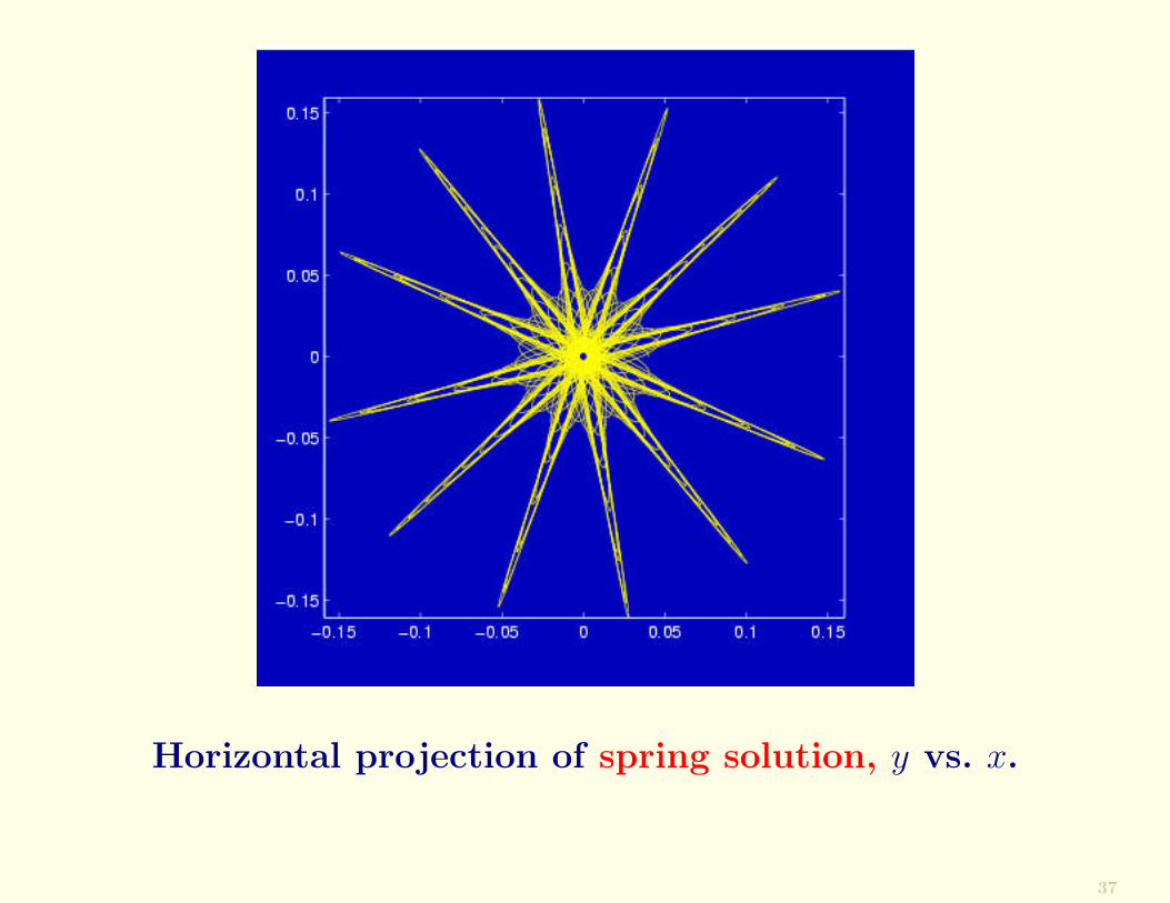
Horizontal projection of spring solution, y vs. x.
37
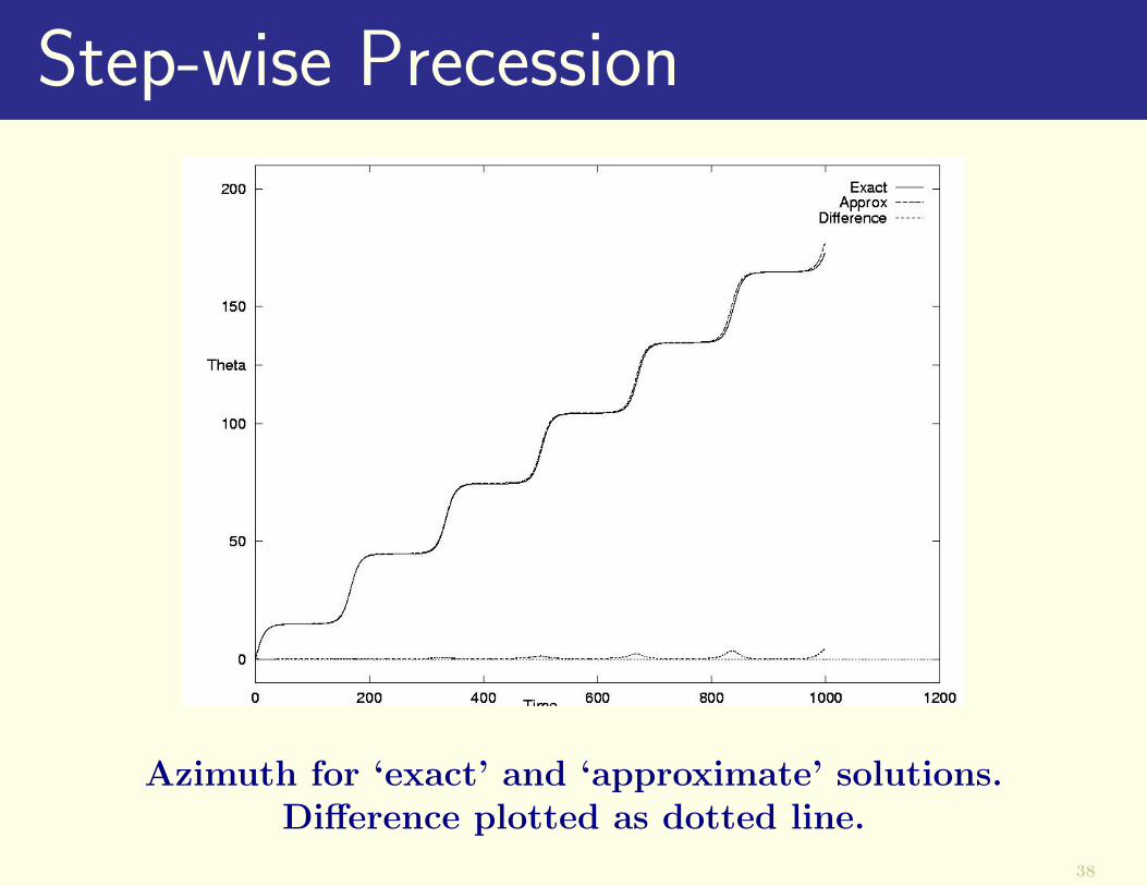
Step-wise Precession
Azimuth for ‘exact’ and ‘approximate’ solutions.Difference plotted as dotted line.
38

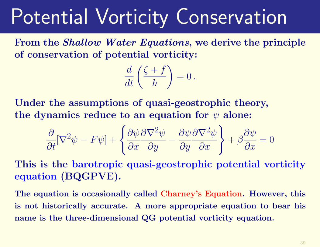
Potential Vorticity ConservationFrom the Shallow Water Equations, we derive the principleof conservation of potential vorticity:
d
dt
(ζ + f
h
)= 0 .
39

Potential Vorticity ConservationFrom the Shallow Water Equations, we derive the principleof conservation of potential vorticity:
d
dt
(ζ + f
h
)= 0 .
Under the assumptions of quasi-geostrophic theory,the dynamics reduce to an equation for ψ alone:
∂
∂t[∇2ψ − Fψ] +
∂ψ
∂x
∂∇2ψ
∂y− ∂ψ
∂y
∂∇2ψ
∂x
+ β
∂ψ
∂x= 0
This is the barotropic quasi-geostrophic potential vorticityequation (BQGPVE).
39
Potential Vorticity ConservationFrom the Shallow Water Equations, we derive the principleof conservation of potential vorticity:
d
dt
(ζ + f
h
)= 0 .
Under the assumptions of quasi-geostrophic theory,the dynamics reduce to an equation for ψ alone:
∂
∂t[∇2ψ − Fψ] +
∂ψ
∂x
∂∇2ψ
∂y− ∂ψ
∂y
∂∇2ψ
∂x
+ β
∂ψ
∂x= 0
This is the barotropic quasi-geostrophic potential vorticityequation (BQGPVE).
The equation is occasionally called Charney’s Equation. However, this
is not historically accurate. A more appropriate equation to bear his
name is the three-dimensional QG potential vorticity equation.
39

Rossby WavesWave-like solutions of BQGPV Equation:
ψ = A cos(kx + `y − σt)
satisfies the equation provided
σ = − kβ
k2 + `2 + F.
This is the celebrated Rossby wave formula
40

Rossby WavesWave-like solutions of BQGPV Equation:
ψ = A cos(kx + `y − σt)
satisfies the equation provided
σ = − kβ
k2 + `2 + F.
This is the celebrated Rossby wave formula
The nonlinear term vanishes for a single Rossby wave:A pure Rossby wave is solution of nonlinear equation.
40

Rossby WavesWave-like solutions of BQGPV Equation:
ψ = A cos(kx + `y − σt)
satisfies the equation provided
σ = − kβ
k2 + `2 + F.
This is the celebrated Rossby wave formula
The nonlinear term vanishes for a single Rossby wave:A pure Rossby wave is solution of nonlinear equation.
When there is more than one wave present, this is no longertrue: the components interact with each other through thenonlinear terms.
40

Resonant Rossby Wave TriadsCase of special interest: Two wave components produce athird such that its interaction with each generates the other.
41

Resonant Rossby Wave TriadsCase of special interest: Two wave components produce athird such that its interaction with each generates the other.
Nonlinear interaction essentially confined to three compo-nents. These three waves are called a resonant triad.
ψ =
3∑n=1
<an(t) exp[i(knx + `ny − σnt)]
Amplitudes an = |an(t)| exp(iϕn(t)) are time-dependent.
Resonant triad must satisfy selection conditions:
k1 + k2 + k3 = 0
`1 + `2 + `3 = 0
σ1 + σ2 + σ3 = 0
41

Pedlosky (1987) used two-timing perturbation approach tostudy resonant triads. The amplitudes of a resonant triadsatisfy
κ21a1 +B1a
∗2a3 = 0
κ22a2 +B2a3a
∗1 = 0
κ23a3 +B3a1a2 = 0
Here κ2n = K2
n + F and K2n = k2
n + `2n, and the interactioncoefficients are
B1 =1
2(k2`3 − k3`2)(K
22 −K2
3) , etc.
42

Conserved QuantitiesThe solutions of the Quasigeostrophic Equation conservenot only the total energy, but also the potential enstrophy.For a wave triad, E and S are constant:
E =1
4
(κ2
1a21 + κ2
2a22 + κ2
3a23
)S =
1
4
(κ4
1a21 + κ4
2a22 + κ4
3a23
)
43

Conserved QuantitiesThe solutions of the Quasigeostrophic Equation conservenot only the total energy, but also the potential enstrophy.For a wave triad, E and S are constant:
E =1
4
(κ2
1a21 + κ2
2a22 + κ2
3a23
)S =
1
4
(κ4
1a21 + κ4
2a22 + κ4
3a23
)Wave components ordered so that
K1 < K3 < K2
This is consistent with arrangment in order of increasingfrequency,
|σ1| < |σ2| < |σ3|
43

Defining
An = µ1µ2µ3
(anµn
), n = 1, 2, 3
where µ2n = |Bn/κ2
n|, the modulation equations are:
A1 = −A∗2A3
A2 = −A3A∗1
A3 = +A1A2
This is the canonical form of the three-wave equations.
44

Defining
An = µ1µ2µ3
(anµn
), n = 1, 2, 3
where µ2n = |Bn/κ2
n|, the modulation equations are:
A1 = −A∗2A3
A2 = −A3A∗1
A3 = +A1A2
This is the canonical form of the three-wave equations.
The Spring Equationsand the
Triad Equations areare
Mathematically Identical!
44

The three-wave equatons are the canonical equations re-sulting from the Hamiltonian H = =A1A2A
∗3, which is a
constant of the motion (Holm and Lynch, 2001).
45

The three-wave equatons are the canonical equations re-sulting from the Hamiltonian H = =A1A2A
∗3, which is a
constant of the motion (Holm and Lynch, 2001).
The energy and enstrophy may be linearly combined to givetwo constants known as the Manley-Rowe quantities:
N1 = |A1|2 + |A3|2 , N2 = |A2|2 + |A3|2 ,
J = |A1|2 − |A2|2 .
This is remarkable:If the energy of the wave with intermediate scale grows,the smaller and larger waves must lose energy.And, of course, vice-versa.
45

Numerical Example of ResonanceImportant scaling property of the three-wave equations:If the amplitudes are scaled by a constant γ and the time iscontracted by a similar factor, the form of the equations isunchanged. Thus, if
A(t) = (A1(t), A2(t), A3(t))
is a solution, then so is
γA(γt) .
Thus, the period of the modulation envelop will vary in-versely with its amplitude.
46

Parameters for Numerical Experiments
a = 4× 10⁷/2πm, Lx = a, Ly = 13a, Nx = 61,
Ny = 21, H0 = 10km, g = π2 ms−2, φ0 = 45and Ω = 2π rad/day. Thus f0 ≈ 10−4 s−1, β ≈ 1.6×10⁻¹¹ m−1s−1,LR ≈ 3× 10⁶ m and F ≈ 10−13 m−2.The means of defining the wavenumbers Kn and frequenciesσn so that the conditions for resonance obtain are discussedby Pedlosky.The wavenumbers (kn, `n) of the three components are givenin the paper. We refer to Wave 3 as the primary component.
47

Components of a resonant Rossby wave triadAll fields are scaled to have unit amplitude.
48

Numerical solution of PDE
∂
∂t[∇2ψ − Fψ] +
∂ψ
∂x
∂∇2ψ
∂y− ∂ψ
∂y
∂∇2ψ
∂x
+ β
∂ψ
∂x= 0
• Potential vorticity, q = [∇2ψ−Fψ] is stepped forward (usinga leap-frog method)• ψ is obtained by solving a Helmholtz equation with peri-odic boundary conditions• The Jacobian term is discretized following Arakawa (toconserve energy and enstrophy)• Amplitude is chosen very small. Therefore, interactiontime is very long.
49
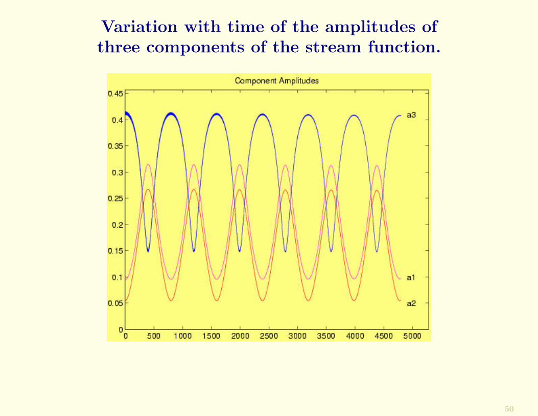
Variation with time of the amplitudes ofthree components of the stream function.
50

Stream function at three times during anintegration of duration T = 4800days.
51

Precession of Triads
• Analogies are Interesting — Equivalences are Useful!
52

Precession of Triads
• Analogies are Interesting — Equivalences are Useful!
Since the same equations apply to both the spring and triadsystems, the stepwise precession of the spring must have acounterpart for triad interactions.In terms of the variables of the three-wave equations, thesemi-axis major and azimuthal angle θ are
Amaj = |A1| + |A2| , θ =1
2(ϕ1 − ϕ2) .
Initial conditions chosen as for the spring (by means of thetransformation relations).Initial field scaled to ensure that small amplitude approxi-mation accurate
52

Polar plot of Amaj versus θ for resonant triad.
Take a peek at the Applet, if available!
53

Horizontal projection of spring solution, y vs. x.
54
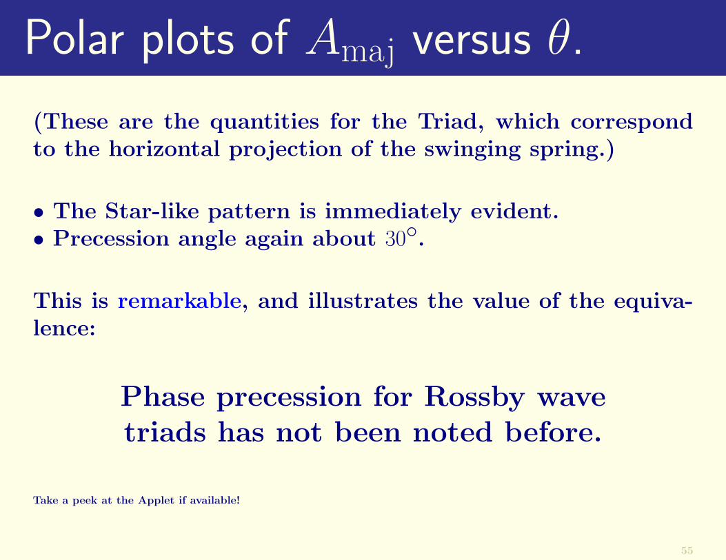
Polar plots of Amaj versus θ.
(These are the quantities for the Triad, which correspondto the horizontal projection of the swinging spring.)
• The Star-like pattern is immediately evident.• Precession angle again about 30.
This is remarkable, and illustrates the value of the equiva-lence:
Phase precession for Rossby wavetriads has not been noted before.
Take a peek at the Applet if available!
55

Rossby Wave Breakdown
• Precession has implications for predictability
• A single Rossby wave may be unstable
• Triad resonance is a mechanism for breakdown
• Highly sensitive to details of minute perturbations
• These are impossible to determine accurately.
56

Initial and final fields for two four-day integrations.Initial fields differ only in the sign of the small perturbation.
57

Predictability
Drastically different patterns can result fromstates which are initially very similar!
This sensitivity is in an integrable systemNo appeal is made to chaos theory!
Refer to BAMS Article (May, 2003) for details.58

Conclusion
I hope I have convinced you that:
This simple system looks like a toy at best, but itsbehaviour is astonishingly complex, with many facetsof more than academic lustre . . .(Breitenberger and Mueller, 1981)
. . . and that the Swinging Spring is a valuable modelof some important aspects of atmospheric dynamics.
59

The End
Typesetting Software: TEX, Textures, LATEX, hyperref, texpower, Adobe Acrobat 4.05Graphics Software: Adobe Illustrator 9.0.2LATEX Slide Macro Packages: Wendy McKay, Ross Moore
![The Arithmetic Geometry of Resonant Rossby Wave Triads · ARITHMETIC GEOMETRY OF RESONANT ROSSBY WAVE TRIADS 353 tion 3.17 and Chapter 6]). The -plane model was introduced by Rossby](https://img.dokumen.tips/doc/110x75/6065c2e71c4a3a76bc3dd2c3/the-arithmetic-geometry-of-resonant-rossby-wave-triads-arithmetic-geometry-of-resonant.jpg)