Embed Size (px)
Citation preview

B O N N E V I L L E P O W E R A D M I N I S T R A T I O N
Residential Heat Pump Water Heater Evaluation: Lab Testing & Energy
Use Estimates
9 November 2011
A Report of BPA Energy Efficiency’s Emerging Technologies Initiative
Prepared for Kacie Bedney, Project Manager Bonneville Power Administration
Prepared by Ben Larson,
Michael Logsdon, David Baylon Ecotope, Inc.
Contract Number 44717

BONNEVILLE POWER ADMINISTRATION November 2011
ii
An Emerging Technologies for Energy Efficiency Report
The following report was funded by the Bonneville Power Administration (BPA) as an assessment of the state of technology development and the potential for emerging technologies to increase the efficiency of electricity use. BPA is undertaking a multi-year effort to identify, assess and develop emerging technologies with significant potential for contributing to efficient use of electric power resources in the Northwest.
BPA does not endorse specific products or manufacturers. Any mention of a particular product or manufacturer should not be construed as an implied endorsement. The information, statements, representations, graphs and data presented in these reports are provided by BPA as a public service. For more reports and background on BPA’s efforts to “fill the pipeline” with emerging, energy-efficient technologies, visit Energy Efficiency’s Emerging Technology (E3T) website at http://www.bpa.gov/energy/n/emerging_technology/projects.cfm.
Ecotope, Inc. is an energy efficiency consulting and engineering firm specializing in the evaluation and design of energy and resource conservation in buildings. Ecotope has specialized in the measurement, evaluation, and development of energy-efficiency programs throughout the Pacific Northwest since 1975. Ecotope is nationally recognized for a strong commitment to high-quality technical analysis, on-going evaluations of energy and resource issues, and sustainable design expertise.
Acknowledgements
The authors would like to thank the entire National Renewable Energy Lab team at the Thermal Test Facility for their high quality work on the project including Dane Christensen, Bethany Sparn, and Kate Hudon.
Abstract
The report describes laboratory testing and modeling exercises performed to assess potential heat pump water heater (HPWH) energy savings in the Pacific Northwest. Three integrated HPWH models, pairing two electric resistance elements with a tank-mound heat pump, were thoroughly investigated: the AO Smith Voltex, the GE GeoSpring, and the Rheem EcoSense. The report summarizes lab findings, describes the determinants of consumption, and develops annual operating efficiency and energy savings estimates for HPWH installations in unheated buffer spaces and interior conditioned spaces throughout the Northwest.

BONNEVILLE POWER ADMINISTRATION November 2011
iii

BONNEVILLE POWER ADMINISTRATION November 2011
iv
Table of Contents
Acknowledgements..................................................................................................................................................... ii
Abstract....................................................................................................................................................................... ii
List of Figures ............................................................................................................................................................vi
List of Tables ........................................................................................................................................................... viii
Executive Summary................................................................................................................................................... ix
1. Introduction ........................................................................................................................................................ 1
1.1. Project Goals ............................................................................................................................................. 1
1.2. Equipment Tested...................................................................................................................................... 2
1.2.1. Equipment Costs ............................................................................................................................... 3
2. Measurement and Verification........................................................................................................................... 4
2.1. Test Setup ................................................................................................................................................. 4
2.2. Test Suite Overview................................................................................................................................... 6
3. Lab Testing Findings ......................................................................................................................................... 8
3.1. Introduction ................................................................................................................................................ 8
3.2. Basic Equipment Characteristics............................................................................................................... 8
3.3. Operating Modes ..................................................................................................................................... 10
3.4. First-Hour Rating and Energy Factor....................................................................................................... 12
3.4.1. First-Hour Rating ............................................................................................................................. 13
3.4.2. Energy Factor .................................................................................................................................. 16
3.5. Equipment COP and Operating Range ................................................................................................... 24
3.5.1. Operating Range ............................................................................................................................. 24
3.5.2. Heat Pump COP .............................................................................................................................. 25
3.6. Air Flow Effects on Performance ............................................................................................................. 30
3.7. Draw Profile and Capacity ....................................................................................................................... 33
3.8. Observations on Equipment Design ........................................................................................................ 36
3.8.1. The AO Smith Voltex ....................................................................................................................... 36
3.8.2. The GE GeoSpring .......................................................................................................................... 37
3.8.3. The Rheem EcoSense..................................................................................................................... 38
4. Energy Use Estimates ..................................................................................................................................... 39
4.1. Overview.................................................................................................................................................. 39
4.2. Constant Parameters and Baseline Inputs .............................................................................................. 40
4.3. Annual Temperature Profiles................................................................................................................... 41
4.3.1. Modeling Approach and Tools......................................................................................................... 41
4.3.2. Building Prototypes.......................................................................................................................... 41

BONNEVILLE POWER ADMINISTRATION November 2011
v
4.3.3. Modeling Assumptions..................................................................................................................... 42
4.4. COP Mapping .......................................................................................................................................... 46
4.5. Garage, Unheated Basement, and Interior Energy Use.......................................................................... 49
4.6. Heating and Cooling System Interactions ............................................................................................... 50
4.6.1. Overview and Qualitative Discussion .............................................................................................. 50
4.6.2. Modeling the Interactions................................................................................................................. 51
4.6.3. Space Heating interactions.............................................................................................................. 52
4.7. Energy Savings Estimates....................................................................................................................... 53
4.8. RTF Energy Use and Savings Estimates ................................................................................................ 56
5. Conclusions ..................................................................................................................................................... 57
5.1. Lessons Learned ..................................................................................................................................... 57
5.2. Equipment Design and Operation ........................................................................................................... 57
5.3. Installation Location Findings .................................................................................................................. 58
References .............................................................................................................................................................. 59
Appendix A. Instrumentation List............................................................................................................................ 60
Appendix B. Graphs................................................................................................................................................ 62
COP Test Results, All .......................................................................................................................................... 64
Draw Profile Tests ............................................................................................................................................... 77

BONNEVILLE POWER ADMINISTRATION November 2011
vi
List of Figures Figure 1. Equipment Tested ..................................................................................................................................... 2
Figure 2. EcoSense Installed in Test Chamber........................................................................................................ 5
Figure 3. GeoSpring Installed in Test Chamber ....................................................................................................... 5
Figure 4. GeoSpring Instrumentation Top View ....................................................................................................... 5
Figure 5. AO Smith Voltex DOE One-Hour Test .................................................................................................... 14
Figure 6. GE GeoSpring DOE One-Hour Test ....................................................................................................... 15
Figure 7. Rheem EcoSense DOE One-Hour Test.................................................................................................. 16
Figure 8. AO Smith Voltex 24-hour Simulated Use Test, Initial Draw Portion........................................................ 18
Figure 9. AO Smith Voltex DOE 24-hour Simulated Use Test, Full 24 hours ........................................................ 19
Figure 10. GeoSpring DOE 24-hour Simulated Use Test, Initial Draw Portion...................................................... 20
Figure 11. GeoSpring DOE 24-hour Simulated Use Test, Full 24 hours ............................................................... 21
Figure 12. Rheem EcoSense DOE 24-hour Simulated Use Test, Initial Draw Portion .......................................... 22
Figure 13. Rheem EcoSense DOE 24-hour Simulated Use Test, Full 24 hours.................................................... 23
Figure 14. Compressor Operating Range Map ...................................................................................................... 25
Figure 15. Voltex COP vs Tank Temperature ........................................................................................................ 26
Figure 16. Voltex COP vs Ambient Temperature ................................................................................................... 27
Figure 17. GeoSpring COP vs Tank Temperature ................................................................................................. 28
Figure 18. GeoSpring COP vs Ambient Temperature............................................................................................ 28
Figure 19. EcoSense COP vs Tank Temperature.................................................................................................. 29
Figure 20. EcoSense COP vs Ambient Temperature............................................................................................. 30
Figure 21. Air Flow Restriction Impacts on Voltex Input Power and Capacity ....................................................... 31
Figure 22. Air Flow Restriction Impacts on GeoSpring Input Power and Capacity................................................ 32
Figure 23. Air Flow Restriction Impacts on EcoSense Input Power and Capacity................................................. 33
Figure 24. Voltex DP-2 Results, Shower Portion ................................................................................................... 34
Figure 25. GeoSpring DP-2 Results, Shower Portion ............................................................................................ 35
Figure 26. EcoSense DP-2 Results, Shower Portion ............................................................................................. 36
Figure 27. Measured and Modeled Garage Temperatures.................................................................................... 44
Figure 28. Garage Annual Temperature Profiles ................................................................................................... 45
Figure 29. Unheated Basement Annual Temperature Profiles .............................................................................. 45
Figure 30. COP Map............................................................................................................................................... 48
Figure 31. Annual Energy Savings with Gas Furnace............................................................................................ 54
Figure 32. Annual Energy Savings with Zonal Resistance Heat............................................................................ 55
Figure 33. Annual Energy Savings with Heat Pump .............................................................................................. 55

BONNEVILLE POWER ADMINISTRATION November 2011
vii

BONNEVILLE POWER ADMINISTRATION November 2011
viii
List of Tables
Table 1. Equipment Cost Data ................................................................................................................................. 3
Table 2. Test Condition Descriptions........................................................................................................................ 6
Table 3. Basic Operating Characteristics ................................................................................................................. 9
Table 4. Equipment Performance Characteristics.................................................................................................. 13
Table 5. Garage Prototype Attached to a 2200-ft2 House...................................................................................... 42
Table 6. Basement Prototype for 2688 ft2 House................................................................................................... 42
Table 7. Garage Heat Transfer Conductances ...................................................................................................... 43
Table 8. Buffer Space Temperature Profiles .......................................................................................................... 46
Table 9. HPWH daily input/output specifications at 67°F and 50% RH ................................................................. 47
Table 10. Annual COP and Energy Use Estimates (HPWH only).......................................................................... 49
Table 11. Annual Space Heating Impacts, Buffer Space Installations ................................................................... 52
Table 12. Annual Space Heating Impacts, Conditioned Space Installations ......................................................... 53

BONNEVILLE POWER ADMINISTRATION November 2011
ix
Executive Summary This report describes laboratory testing and modeling exercises performed to assess potential heat pump water heater (HPWH) energy savings in the Pacific Northwest. Three HPWH models available to consumers at the project’s inception were thoroughly investigated: the AO Smith Voltex, the GE GeoSpring, and the Rheem EcoSense. Each water heater is an integrated device pairing two electric resistance heating elements with a tank-mounted heat pump.
With little cooling load and generally low to moderate temperatures, Northwest climates are not always ideal for HPWHs, but healthy, reliable energy savings are still possible through a careful selection of equipment and installation locations. In particular, successful and efficient heat pump operation at low ambient temperatures is required. Many installations occur in unconditioned buffer spaces that experience cool temperatures much of the year. The compressor must function efficiently under these conditions for the HPWH to be a sound electricity-savings investment.
The combined lab and modeling results suggest the determinants of efficient HPWH operation:
1. Resistance element runtime and operational strategies. For these HPWHs, with multiple heating sources and operational strategies that switch between them, anytime the resistance element runs, there is no energy saved over a base case tank.
2. Compressor characteristics including efficiency, operating range, and capacity. High coefficients of performance (COPs) when the heat pump operates are a necessary condition to generate savings. The ambient temperature operating range sets the limits within which the compressor will run. The compressor COP and output capacity then determine how quickly the tank can recover from a draw while remaining in the efficient, heat pump only mode.
3. Tank storage volume relative to hot water load. When considered in conjunction with resistance element operation and compressor characteristics, larger tanks can offer efficiency advantages. Larger tanks may be drawn down further before invoking resistance heat. Further, when heat pump output capacity is low due to smaller compressor size or colder ambient conditions, more tank storage results in delaying the activation of the resistance heat elements, allowing the heat pump to do more heating of the water.
4. Ambient air temperature surrounding the HPWH. Ambient temperature impacts the refrigeration cycle heating efficiency in the familiar ways of improved performance at higher temperatures. Additionally, the installation location may have periods of time where the temperature is outside the operating range of the compressor, forcing the equipment into resistance heating.
The three models evaluated exhibited different results with respect to the determinants of efficient operation. Resistance element control strategies, compressor operating ranges, and capacities all varied between equipment:
1. The Voltex compressor operated over the widest temperature range, while the control strategies worked to reduce the resistance element runtime. The generous tank size enabled the unit to take advantage of heat pump efficiency.
2. The GeoSpring operating range is somewhat less than the Voltex, and the compressor, although the most efficient tested, is limited by its size. Combined with a smaller tank size, those features can lead to increased resistance heat runtimes.
3. The EcoSense heat pump experiences coil frosting at mild ambient temperatures, making it unsuitable for buffer space applications in the Northwest climate. Successful steady-state compressor operation was not observed below 57°F. In addition, the EcoSense mixes the tank water, an artifact of its condenser

BONNEVILLE POWER ADMINISTRATION November 2011
x
heat exchanger, disrupting the temperature stratification that is crucial for maintaining hot water output during repeated draws.
Installation location is, in itself, a complex issue in climates where the heating season dominates. Placing the HPWH in an unconditioned buffer space, such as the garage, reduces heat pump efficiency because the compressor must work against a larger temperature difference. Placing the HPWH inside a conditioned space adds to the space heating load. This lack of an obvious, optimum installation location necessitated the measurements and modeling described in the report. The analysis of installation locations showed:
1. Garage installations, especially in marine climates and depending on the equipment, are desirable locations for producing energy savings. As a buffer space, the garage is decoupled from the house heating system, so interactive effects are greatly reduced. Equipment with a wide enough operating range can take advantage of the “free” heat from natural air infiltration, solar gains, and ground contact to heat the water efficiently.
2. Unheated basement installations, as another buffer space location, showed savings as well but often exhibited somewhat lower potential than garages due to tighter coupling to the house heating system.
3. Interior installations across the region for houses with gas or heat pump space heating also produce high electric savings. Gas-heated houses end up using more gas heat in this scenario to make up the energy the water heater extracts from the house. Heat-pump houses produce a high level of savings because they effectively create a two-stage compressor system moving heat from outdoors to indoors to the water tank.
Overall, the project demonstrated estimated energy consumptions indicating that HPWHs can be a viable source of energy savings. Although the savings can vary considerably based on the equipment, installation location, and climate, there are a number of combinations that will lead to reduced energy usage over a traditional resistance-only hot water tank.

BONNEVILLE POWER ADMINISTRATION November 2011
1
1. Introduction
In the Pacific Northwest, the dominant technology used to heat domestic hot water (DHW) consists of electric resistance elements in an insulated tank. This option is the most common type of water heating system in the residential sector with 64% of all single family houses using such tanks amounting to approximately 3.5 million units (NPCC 2010). Over the last twenty years, the quantity of insulation required in electricity-heated DHW tanks has steadily increased. These improved tank insulation standards have reduced the standby loss of heat from the tank by a factor of two. Unfortunately, the impact of these efficiency improvements on the overall energy use of the DHW tank is minimal because the amount of energy needed to heat the water demanded by the house has remained relatively constant.
Beginning in the 1980s, companies in the region experimented with heat pump technologies to meet the energy demand from DHW using heat pump water heater (HPWH) technology (Hanford 1985). In several efforts, the technical and/or market challenges proved insurmountable. In the last five years, however, several major manufacturers have designed and introduced HPWH products. These efforts have the backing of mainstream equipment makers with large and well established distribution and marketing networks.
This project sought to answer the technical questions associated with these new generation residential HPWHs. Issues that surfaced in previous studies, including water heater placement, equipment design, and overall performance, were addressed by using laboratory testing and thermal simulation modeling. This approach has the advantage of providing tests with known parameters so performance can be monitored given the conditions under which the HPWHs may operate in Pacific Northwest applications.
The lab testing protocols were designed with consideration to the important operating and interaction characteristics that are present for an HPWH installation in the Pacific Northwest. The lab tests lay the foundation for building simulation models that are necessary to quantify the interactions with a particular house space conditioning system. By considering the interaction of the HPWH with the house, the full energy impact of an installation can be determined.
The project assessed three HPWHs from three manufacturers currently bringing a product to market. Each of these units is designed as a “drop-in” replacement for an existing electric water heater. The units are integrated, consisting of a tank, compressor, and resistance element heating. The project focused on assessing the equipment design and the house installation parameters needed to achieve optimum energy savings, as well as performance over a range of operating conditions.
1.1. Project Goals
The project goals were focused on identifying the factors that would determine the energy use and energy efficiency of three specific HPWHs. This goal was divided into four tasks:
1. Using a controlled laboratory environment, evaluate the performance of HPWHs in Pacific Northwest conditions. The evaluation allowed for the development of a full range of performance characteristics of the HPWH equipment for ambient temperature conditions and DHW loads.
2. Determine impacts of the HPWHs on the spaces where they are installed, including potential space heating and cooling interactions.
3. Estimate electric energy savings and savings determinants for HPWH applications. These include the impact of equipment placement in the house and the impact of regional climate variations.

BONNEVILLE POWER ADMINISTRATION November 2011
2
4. Assess energy savings potential as a function of the equipment performance of the HPWH models, and show conditional impacts of the HPWHs based on effective coefficient of performance (COP) and placement in the home.
1.2. Equipment Tested The following three HPWHs were tested for this project:
AO Smith Voltex Hybrid1 model # PHPT-80
GE GeoSpring2 model # GEH50DNSRSA
Rheem EcoSense Hybrid3 model # HP50RH
Figure 1. Equipment Tested
Note: images not to scale.
All three models are currently for sale and available in the United States. The Voltex tested has an 80-gallon tank, and the GeoSpring and EcoSense units have 50-gallon tanks. There is also a 60-gallon version of the Voltex and a 40-gallon version of the EcoSense, which have similar designs and component configurations but were not evaluated in this project. The Bonneville Power Administration (BPA) arranged for the acquisition of all the test equipment. The GeoSpring test equipment was purchased as an “off-the-shelf” unit at a large home improvement retailer near the testing lab. The EcoSense test equipment was supplied directly by the manufacturer. The Voltex test equipment was obtained through a plumbing wholesale distributer in the Portland area and shipped to the testing lab.
1 Image source: http://www.hotwater.com/water-heaters/residential/hybrid/voltex/ 2 Image source: http://products.geappliances.com/ApplProducts/Dispatcher?REQUEST=SpecPage&Sku=GEH50DNSRSA#WEIGHTS%20&%20DIMENSIONS 3 Image source: http://www.homedepot.com/buy/plumbing/water-heaters/rheem-ecosense/50-gal-hybrid-electric-water-heater-with-heat-pump-technology-42207.html

BONNEVILLE POWER ADMINISTRATION November 2011
3
1.2.1. Equipment Costs
As can be expected with emerging technologies and new products, the equipment prices fluctuated somewhat during the project timeline. In mid-2011, the prices were surveyed and are reported in Table 1. Sample costs for same-sized resistance tanks are included as baselines for comparison. In addition to the purchase price difference between the HPWH and the baseline tank, there are incremental installation costs for the HPWH. Plumbers must address the condensate drainage path on the HPWH and may also need to configure different inlet and outlet piping arrangements.
Equipment Cost Data
Item Cost (2011 $'s) Source Notes Voltex 80-gal $ 2,024 lowes.com HPE2K80HD045V
Voltex 60-gal $ 1,653 lowes.com Whirlpool Model #:HPE2K60HD045V
GeoSpring 50-gal $ 1,400 sears.com
EcoSense 50-gal $ 1,298 homedepot.com
Baseline 80-gal $ 469 homedepot.com 0.86 EF - GE80T06AAG
Baseline 60-gal $ 444 lowes.com 0.90 EF - Whirlpool Model #:E2F65HD045V
Baseline 50-gal $ 254 homedepot.com 0.90 EF - GE50M06AAG
Incremental Install $ 140 HPWH: BPA/EPRI study costs; Std Tank: 3 contractor estimates
Table 1. Equipment Cost Data
The HPWHs are also sold with warranties on the tank and parts of 10 years for the Voltex,4 10 years for the GeoSpring,5 and 12 years for the EcoSense.6
4 http://www.hotwater.com/water-heaters/residential/hybrid/voltex/
5 http://products.geappliances.com/ApplProducts/Dispatcher?REQUEST=SpecPage&Sku=GEH50DNSRSA
6 http://www.homedepot.com/buy/plumbing/water-heaters/rheem-ecosense/50-gal-hybrid-electric-water-heater-with-heat-pump-technology-42207.html

BONNEVILLE POWER ADMINISTRATION November 2011
4
2. Measurement and Verification Working with BPA and an Advisory Committee of regional HPWH stakeholders, Ecotope developed a laboratory measurement and verification (M&V) plan. The full plan is available on the BPA website: http://www.bpa.gov/energy/n/emerging_technology/pdf/HPWH_MV_Plan_Final_012610.pdf
With the M&V plan in place, Ecotope conducted a broad search to find a lab to conduct the measurements. In conjunction with BPA, Ecotope selected the National Renewable Energy Laboratory (NREL) in Golden, Colorado, to carry out the M&V plan. NREL is a nationally recognized lab with extensive experience testing both water heating and heat pump systems. The tests were conducted in NREL’s Advanced Thermal Conversion Laboratory within the Thermal Test Facility. NREL put the M&V plan into action and carried out the testing in consultation with Ecotope. Although NREL conducted the measurements and provided the data, any conclusions in the report are those of the report authors and not the test facility.
2.1. Test Setup
NREL constructed a thermally isolated and temperature/humidity-controlled chamber capable of testing two HPWHs side-by-side. A sophisticated set of controls in a feedback loop was used to supply the chamber with tempered air to maintain the ambient conditions around the water heaters at the desired levels. A series of fans, cooling coils, and heating elements were continuously used to condition and trim the temperature and moisture content of the incoming air. The air was also continuously moved through the chamber in order to isolate the water heater interaction from the surrounding environment and also allowed two water heaters to be tested concurrently. Figure 2 shows the test chamber with the access door open and a test unit installed. The door was closed during testing. Figure 3 shows another test unit in the chamber. One of the chamber outlet air ports can be seen at the bottom left of the photo.
Tempered water was conditioned and stored in a large tank to be supplied to the water heaters at the desired inlet conditions. Additionally, NREL installed a dump valve just upstream of the tank inlet so that any water that did not meet the inlet temperature specification would be cleared from the supply line prior to any draw.
NREL installed an instrumentation package to measure the required points specified by the U.S. Department of Energy (DOE) test standard as well as additional points to gain further insight into HPWH operation. The tank water temperature was measured with a tree of six thermocouples positioned at equal water volume segments. Inlet and outlet water temperatures were measured with thermocouples immersed in the supply and outlet lines. Three thermocouples were mounted to the surface of the evaporator coil at the refrigerant inlet, outlet, and midpoint to monitor the coil temperature to indicate the potential for frosting conditions. Power for the equipment was independently monitored for the entire unit, compressor, fan, and, in one case, the pump. Appendix A provides a complete list of sensors, which includes more than those mentioned here, plus their rated accuracies.
Warranting special mention is the airflow across the water heater evaporator coils, which was measured with a nozzle box and set of laminar flow elements. The inlet air came from the test chamber. The outlet air was not exhausted to the chamber but rather was captured in custom-built discharge plenums and ducted to the nozzle box. Figure 4 shows an example of the discharge plenum. An inline booster fan was used to maintain the same static pressure for the evaporator fan as would be experienced in standard, free-air, discharge conditions. Further, as the lab is situated at over 5,000 feet in altitude, the booster fan was used to simulate the same air mass flow conditions for standard atmospheric conditions at sea-level elevations.

BONNEVILLE POWER ADMINISTRATION November 2011
5
Figure 2. EcoSense Installed in Test Chamber Figure 3. GeoSpring Installed in Test Chamber
Figure 4. GeoSpring Instrumentation Top View

BONNEVILLE POWER ADMINISTRATION November 2011
6
2.2. Test Suite Overview
The M&V plan test suite contained five broad areas of testing:
1. Operating Mode – sought to describe control logic, revealing conditions at which the heat pump or resistance elements activated.
2. DOE Standard Rating Point Tests – conducted as part of the standard suite of tests used to label the equipment.
3. Supplemental Draw Profiles – designed by Ecotope to further capture the flavor of performance for each HPWH.
4. COP Curve Development – Performance Mapping – provided information used in modeling the overall energy impact of the HPWH, including both usage and space heating interactions.
5. Airflow – investigated the performance degradation of a clogged air filter.
Table 2 summarizes the conditions under which each test was conducted. For complete descriptions of each test, refer to the full Measurement and Verification Plan.
Ambient Air Water Test Name
Dry bulb (F) RH Inlet (F) Outlet (F)Airflow Operating Mode
1. Operating Mode Characterization Tests OM-67 67.5 50% 58 135 100% All Factory Modes OM-95 95 40% 58 135 100% Hybrid Modes OM-47 47 73% 58 135 100% Hybrid Modes
2. DOE Standard Rating Tests DOE-1hr 67.5 50% 58 135 100% Factory Default
DOE-130-1hr 67.5 50% 58 130 100% Factory Default DOE-140-1hr 67.5 50% 58 140 100% Factory Default
DOE-24hr 67.5 50% 58 135 100% Factory Default 3. Draw Profiles
DP-2 67.5 50% 45 120 100% Factory Default DP-3 67.5 50% 45 120 100% Factory Default
4. COP Curve Development – Performance Mapping COP-47 47 73% 35 135 100% Compressor Only COP-57 57 61% 35 135 100% Compressor Only COP-67 67.5 50% 35 135 100% Compressor Only COP-77 77 40% 35 135 100% Compressor Only COP-85 85 42% 35 135 100% Compressor Only COP-95 95 40% 35 135 100% Compressor Only
COP-95 dry 95 20% 35 135 100% Compressor Only COP-105 105 42% 35 135 100% Compressor Only
COP-105 dry 105 16% 35 135 100% Compressor Only 5. Airflow – Performance Mapping
AF-1/3 67.5 50% 35 135 66% Compressor Only AF-2/3 67.5 50% 35 135 33% Compressor Only
Table 2. Test Condition Descriptions

BONNEVILLE POWER ADMINISTRATION November 2011
7
With HPWH operation parameters determined by the lab test results, the M&V plan called for using those outputs to determine the space heating/cooling interactions of the equipment. The interactions were not tested directly; rather, they were found by applying the test results in a thermal model. Testing output provided data for performance curves, which calculated both the energy required to heat the water and the heat removed from the space. Modeling is needed to fully characterize the space interaction because HPWH efficiency depends on ambient temperature, which itself is impacted by the HPWH. The water heater use also varies with time. To truly capture these effects, an interactive model is needed. The full analytical calculations are discussed in section 4 after the lab results are presented in section 3.

BONNEVILLE POWER ADMINISTRATION November 2011
8
3. Lab Testing Findings
3.1. Introduction
As described above in section 2, the AO Smith Voltex, GE GeoSpring, and Rheem EcoSense were evaluated in accordance with the M&V plan at NREL in Golden, Colorado. This portion of the report discusses operation and performance of the equipment itself. The purpose is to understand and document how the equipment works in a controlled setting. Subsequent sections of the report apply the results to various installation scenarios.
3.2. Basic Equipment Characteristics
The AO Smith Voltex Hybrid model # PHPT-80, GE GeoSpring model # GEH50DNSRSA, and Rheem EcoSense Hybrid model # HP50RH are electric water heaters consisting of a heat pump integrated with a hot water tank. Each model has two methods of heating water:
1. Extracting energy from the ambient air and using the heat pump to transfer the energy to the water.
2. Activating resistance heating elements immersed within the tank.
The heat pump compressor and evaporator are located atop the tank for each of the three models. The Voltex evaporator fan, axial and single-speed, draws ambient air from the left side of the unit (when viewing the control panel) through a washable filter and across the evaporator coils, and exhausts cooler air out the right side. The EcoSense evaporator fan, similarly single-speed, draws ambient air from the top of the unit, through a washable filter and across the evaporator coils, and exhausts cooler air out the sides. In contrast, the GeoSpring evaporator contains two, variable-speed, axial fans. These fans draw ambient air in from the upper sides of the unit and across the evaporator coils, and exhaust cooler air out the back.
The condenser coils, which transfer heat from the refrigerant to the water, wrap around the outside of the tank in the Voltex and GeoSpring models. The EcoSense condenser rests above the tank and exchanges heat by circulating water pumped from the bottom of the tank, and so the pump must operate in conjunction with the compressor. This heat exchanger is coaxial – a tube within a tube.
The lab conducted measurements to develop a basic, descriptive characterization of the equipment. These measurements are presented in Table 3 and discussed in the rest of this section. For comparison purposes, the table shows both measured values and values provided by the manufacturer’s specifications.

BONNEVILLE POWER ADMINISTRATION November 2011
9
GE GeoSpring Rheem EcoSense AO Smith Voltex
Units Lab Meas.Spec. Sheet
Lab Meas.Spec. Sheet
Lab Meas. Spec. Sheet
Upper* Element kW 4.5 2.5 2.5 4.5
Lower* Element kW 4.5 2.5 2.5 2.0
Compressor** Power W 300-700 700 450-1100 -- 550-1100 700
Standby Power W 3 2 8 -- 8 --
Fan*** Power W 5-10 -- 11 -- 85 --
Pump Power W na na 73 -- na na
Airflow Path
Inlet on sides. Exhaust to back.
Inlet on top. Exhaust to sides.
Inlet on left side. Exhaust to right side.
Airflow cfm 100-175 -- 100 -- 475 --
Refrigerant R-134a R-410a R-134a
*240V supply. Elements interlocked for GeoSpring and Voltex, may operate in tandem for EcoSense.
**range depends on water T and ambient T. Power increases with each.
***variable speed for GeoSpring - depends on conditions
Units of measure: kW = kilowatts; W = watts; cfm = cubic feet per minute
Table 3. Basic Operating Characteristics
As with traditional electric water heaters, the three hybrid models studied each have two resistance heating elements, one upper and one lower. At 240 Volts, the Voltex upper element draws 4.5 kW and the lower element draws 2.0 kW. The GeoSpring resistance elements each draw 4.5 kW. With these models, only one element may operate at any given time. The EcoSense resistance elements each draw 2.5 kW at 240 Volts, but are allowed to operate simultaneously. This creates a total equipment draw of 5.0 kW.
The controls for all three models effectively limit total equipment power draw. Of the three heating components—compressor, upper resistance element, and lower resistance element—the Voltex and GeoSpring allow only one to operate at any given time. There is no concurrent operation of heating sources. Measurements show that the Voltex compressor draws 550-1100W and the GeoSpring compressor draws 300-700W, depending on tank temperature and ambient conditions, leaving the equipment maximum for both as 4.5kW, the maximum resistance element power draw.
The EcoSense, in contrast, is allowed to operate its compressor either alone or in conjunction with a single resistance element. Measurements show the compressor draws 450-1100W, depending on tank temperature and ambient conditions, leaving the combined compressor and resistance draw well below the equipment maximum of 5.0 kW from simultaneous operation of both resistance elements (recall the EcoSense elements draw only 2.5 kW each).
The evaporator fan and control circuits induce additional power draw, with sundry extra draws depending on model. The Voltex evaporator fan moves 475 cfm and draws 85W. Its control circuits use 8W constantly. The Voltex also employs a powered anode rod to protect against corrosion, which draws 50 milliamperes (mA) maximum (about 6W). This value was not measured separately in the lab, so its power use is not confirmed.
The GeoSpring variable speed fans move 100-175 cfm and draw 5-10W, depending on conditions, and its control circuits use 3W constantly. These are the only additional power draws for the GeoSpring.

BONNEVILLE POWER ADMINISTRATION November 2011
10
The EcoSense employs a pump to pass cool water from the bottom of the tank through the condenser at the top of the tank. The heat exchanger is coaxial—a tube within a tube—so tank water must flow through the exchanger to gain heat from the refrigerant. This pump draws 73W. The EcoSense fan moves 100 cfm and draws 11W, and its control circuits use 8W continuously. Curiously, the pump was observed to continue operation even after the compressor shut down. This was true with either a single resistance element or both resistance elements operating concurrently. The implications of this are discussed later.
Tank capacity was measured for each model. The Voltex is rated at 80 gallons of capacity, and the unit in the lab held 75.0 gallons. Similarly, the GeoSpring nominally holds 50 gallons, and the unit in the lab held 45.5 gallons; the EcoSense nominally holds 50 gallons, and the unit in the lab held 45.3 gallons. National guidelines on the sizing of equipment allow a 10% variation in nominal versus actual size, and therefore, despite their reduced actual capacities, all three models still fall within this acceptable range. It should be noted that the difference in nominal size versus actual size is not unique to HPWHs and occurs with traditional electric resistance tanks as well.
Also of note in regard to the Voltex is that, due to its increased capacity, it is larger than the other units or most conventional residential DHW systems. To hold 75 gallons of water and accommodate heat pump components, the Voltex is 81.5 inches tall with a 24.5-inch diameter. The GeoSpring measures 60.5 inches tall with a 24-inch diameter. The EcoSense measures 75.5” tall with a 21” diameter.
Lastly, the Voltex and GeoSpring use R-134a refrigerant, and the EcoSense uses R-410a refrigerant which is typically used in split-system space conditioning heat pumps. R-134a condenses at higher temperatures than R-410a, which allows compressor heating to achieve a higher setpoint. The R-134a systems heat the tank to 140°F without the need for supplemental heat. In the tests, the EcoSense compressor using R-410a heated water to ~132°F before switching to resistance heat.
3.3. Operating Modes
Traditional electric water heaters use two resistance heating elements to heat the tank. Thermostats control the operation of the elements which are located at different heights in the tank. A typical operating strategy for the tanks is to engage the lower element first as it detects cooler water filling the tank from the bottom. Then, as the level of cold water rises, the upper element activates (while the lower switches off) to heat the top layer of water in the tank. When the top of the water column reaches the setpoint, the upper element shuts down and the lower element reactivates, heating the remainder of the tank.
Each HPWH has an integrated circuit control board that can be programmed to direct heating component usage patterns—that is, rules for when to activate and deactivate the compressor and resistance elements. Each manufacturer developed several control strategies, referred to as operating modes, to determine these patterns of equipment operation. The general trend is to offer an array of modes, bookended by one of maximal compressor usage and one of maximal resistance heating usage. The details vary somewhat between models. The specific modes for each model are summarized as follows:
1) Voltex a) Efficiency – Compressor operation only, provided ambient temperature is in the range of 45°F – 109°F
and tank temperature is above 58°F. b) Hybrid – Combination of compressor and resistance elements. c) Electric Only – Resistance elements only with either lower or upper element.
2) GeoSpring a) eHeat – Compressor only, unless evaporator coil frosting occurs. b) Hybrid – Combination of compressor and resistance elements.

BONNEVILLE POWER ADMINISTRATION November 2011
11
c) High demand – Combination of compressor and resistance elements, favoring the resistance elements. d) Electric only – Resistance elements only with either lower or upper element.
3) EcoSense a) Energy Saver – Combination of compressor and resistance elements. b) Normal – Combination of compressor and resistance elements, with the resistance elements activating
more quickly in response to demand than in Energy Saver mode. c) Electric Heat Only – Resistance elements only with lower, upper, or both elements.
As specified in the operating mode characterization section of the M&V plan, the lab performed tests exploring the specifics of each control strategy. Each test began with the water heater full of water at a setpoint of either 120°F or 140°F. A draw was initiated and continued until the compressor turned on (if possible for that mode of operation). The draw was then stopped and the unit was allowed to recover. A second draw was performed for the same air temperatures, humidity conditions, and tank setpoint. This second draw was allowed to continue until the resistance heaters came on or until 40 gallons of water had been drawn (70 gallons for the 80-gallon tank). The units were then allowed to recover. The same procedure was followed for different ambient air temperatures of 47°F, 67°F, and 95°F dry bulb spanning the set of operating modes.
Of the three equipment models tested, the manufacturer of the Voltex (AO Smith) provided the most information and the clearest description of their operating modes. The Voltex has two thermistors mounted on the exterior of the tank but underneath the insulation. The upper thermistor covers about the top one-sixth of the tank volume, and the lower thermistor covers about the lower one-third of the tank volume. The equipment then monitors the upper temperature, the lower temperature, and a combination of the two described by the following equation:
Note that this does not represent average tank temperature. It is used only as a reference tank temperature on which to base control decisions.
For the GeoSpring, the lab observed that the primary source of heating component control is a temperature sensor near the upper heating element, approximately one-fourth of the volume below the top. For the EcoSense, the lab found that the primary source of control is a thermocouple located near the lower element in the tank, roughly three-fourths of the volume below the top.
During these tests, the following observations were recorded:
1) Voltex a) Efficiency Mode: The compressor is used exclusively in this mode and turns on when Ttank,Voltex falls 9°F
below setpoint and remains on until the tank achieves setpoint. If the ambient temperature is beyond the operating bounds of 45°F to 109°F or if Ttank,Voltex is less than 58°F, the resistance elements heat the tank after water draws.
b) Hybrid Mode: This mode blends heat pump and resistance element operation while favoring the heat pump. The compressor turns on when Ttank,Voltex falls 9°F below setpoint and remains on until the tank achieves setpoint. For larger draws, where Ttank,Voltex falls 18-20°F below setpoint, the upper resistance element turns on and the compressor shuts off. If the upper resistance element is activated in this way, it will run until setpoint is met at the upper thermistor before shutting off and letting the compressor finish heating the tank.
c) Electric Only Mode: Only the electric resistance elements are used in this mode. A drop of 5°F in Ttank,Voltex activates the upper element. When the upper temperature recovers, the lower element switches on to finish heating the tank.

BONNEVILLE POWER ADMINISTRATION November 2011
12
2) GeoSpring a) eHeat Mode: This mode uses only the compressor, unless the ambient temperature is beyond the
operating bounds of 45°F to 120°F or if coil icing is imminent. The compressor turns on when a slight temperature change is detected at a sensor near the upper resistance element (roughly the top one-fourth volume of the tank), and remains on until the tank achieves setpoint.
b) Hybrid Mode: This mode blends heat pump and resistance element operation. The compressor turns on when a slight temperature change is detected near the upper resistance element and remains on until the tank achieves setpoint. During larger draws, a 10-20°F drop near the upper resistance element causes the compressor to shut off and the upper resistance element to turn on and run until the top of the tank is back at setpoint. The HPWH will then switch to the lower resistance element to finish heating the tank. Once the resistance elements have been activated, the HPWH uses resistance heat only to finish heating the tank. The compressor does not start up again until the next draw cycle.
c) High Demand Mode: This mode is similar to Hybrid Mode but with a greater propensity to use the resistance elements. A slight temperature change triggers the compressor to turn on, but a continued drop of greater than ~5°F in the water surrounding the temperature sensor will trigger the lower element (not the upper) to activate first. The upper element will subsequently cycle on. As in hybrid mode, once the resistance elements have been activated, the compressor is not used again until the next draw cycle.
d) Electric Only Resistance Mode: Only the electric resistance elements are used in this mode. When a draw is initiated and a change in the upper tank temperature sensor is detected, the upper element turns on. Once the top of the tank reaches the setpoint, the unit switches back to the lower element until the tank re-attains the setpoint.
3) EcoSense a) Energy Saver Mode: This control strategy favors the operation of the compressor and at most one
resistance element, unless ambient conditions dictate compressor shut down due to frosting. In that case, both resistance elements are used while the compressor is off (the only scenario in which both resistance elements are used in Energy Saver Mode). Otherwise, the compressor is first to activate in response to falling tank temperature from a water draw. If the thermocouple senses a water temperature drop to ~70°F or colder, the compressor engages. For higher setpoints (140°F), the upper element subsequently activates if the tank temperature deviates too far from the setpoint. To complete the upper end of the heating cycle, for tank temperatures above 130°F, a single resistance element tops off the tank temperature (recall that the EcoSense uses R-410a refrigerant, which allows compressor-based heating only up to about 130°F). If the evaporator coil starts frosting, the compressor switches off and both resistance elements activate. Once this has happened three times in a cycle, the HPWH uses resistance heat exclusively for the duration of the recovery.
b) Normal Mode: This mode is similar to Energy Saver. The only discernable difference is that the unit reverts to all electric for slightly longer at the end of each recovery cycle.
c) Electric Heat Only: Only the resistance elements are used in this mode. Both resistance elements activate in response to a water draw. The upper element shuts off when the top of the tank achieves setpoint, and the lower element remains on to finish heating the tank.
3.4. First-Hour Rating and Energy Factor
To rank the comparative performance of HPWHs, the DOE has established two tests. One test produces a first-hour rating, expressing how much useable hot water the heater produces in one hour. The other, a 24-hour simulated use test, produces an energy factor (EF), which is calculated by dividing the heat inherent in the delivered hot water by the amount of energy consumed over a 24-hour usage pattern. For tank-type water heaters, the first-hour rating depends largely on tank volume and heating output capacity. The EF depends on the heating system efficiency and the heat loss rate of the tank. The normative performance characteristics of the

BONNEVILLE POWER ADMINISTRATION November 2011
13
equipment are shown in Table 4 and discussed in the rest of this section. Although the lab carried out the tests in alignment with the DOE specification, the outputs here should not be considered official ratings – those are the ones reported by the manufacturer.
GE GeoSpring Rheem EcoSense AO Smith Voltex
Units Lab Meas.Spec. Sheet
Lab Meas.Spec. Sheet
Lab Meas. Spec. Sheet
Test Mode Hybrid Energy Saver Hybrid
Tank Volume gal 45.5 50 45.3 50 75 80
First-Hour Rating gal 57 63 37.5 67 87 84
Energy Factor EF 2.41 2.35 1.69 2 2.29 2.33
Tank Heat Loss Rate Btu/hr-F 3.8 -- 5.1 -- 3.9 --
Table 4. Equipment Performance Characteristics
The lab conducted both the 1-hour and 24-hour tests to demonstrate repeatability with the manufacturer’s data. All tests were performed in each manufacturer’s default mode upon shipping. The information generally agreed with the manufacturer’s published ratings, except in the case of the EcoSense. The lab measurements for both the first-hour rating and the EF were less than the manufacturer’s published specifications. That discrepancy is discussed in sections 3.4.1 and 3.4.2.
3.4.1. First-Hour Rating
The first-hour rating test generates one primary quantity: gallons of hot water supplied by the heater in one hour. The quantity can be useful in sizing a tank for household peak demand situations. The test starts with a full, hot tank (135°F) of water and proceeds with a 3 gallons per minute (gpm) draw. The first draw continues until the outlet water temperature falls 25°F below the tank starting conditions. The tank is then allowed to recover. As the heating components switch off (or from upper to lower), indicating available hot water at the top of the tank, a draw is initiated again until the outlet water temperature falls to a similar temperature of the first draw minimum. The cycle is repeated until the 60-minute mark when one last draw is conducted. Throughout the test, only outlet water with a temperature above cutoff temperature for the first draw is counted in the final volume. The test result is first a function of tank capacity and second of heating capacity. Lastly, in HPWH systems with two heating methods, using the highest output capacity heating components will result in the highest output rating.
The Voltex
The data from the Voltex one-hour test at 135°F setpoint are plotted in Figure 5. Approximately five minutes into the first draw, the heat pump activated (green line showing 0.8kW). As the draw continued past 20 minutes, the Ttank fell far enough below setpoint (18°F) to engage the upper heating element (green line to 4.5kW), turning off the compressor in the process. At 55 minutes, the upper portion of the tank recovered to setpoint, so the equipment switched to the compressor. Per the DOE test method, this triggered another draw because the water at the top of the tank was then hot. The draw continued past minute 60 when the resistance element engaged again. Shortly thereafter, the test was terminated.

BONNEVILLE POWER ADMINISTRATION November 2011
14
Figure 5. AO Smith Voltex DOE One-Hour Test
The GeoSpring
The data from the GE GeoSpring one-hour test are plotted in Figure 6. Approximately five minutes into the first draw, the HPWH compressor turned on (green line showing about 400W). As the tank temperature fell further, the upper resistance element turned on (green line to 4.5kW) to satisfy the increasing demand. One of the two resistance elements stayed on for the remainder of the test. Even under the most optimal ambient conditions, the resistance heat element of this water heater will provide more capacity than the heat pump compressor. Therefore, to maximize output (at the expense of efficiency), the resistance elements are favored in this test. Interestingly, the DOE standard does not specify which heating methods (resistance or heat pump) shall be used in the pre-test tank conditioning. The water draw the lab used to “establish normal water heater operation” was a deep enough one which ended up triggering the resistance elements and not the heat pump. When the tank cut-out from this recovery, the lowest thermocouple (lowest one-sixth of tank) was left reading a temperature of 100°F. Had the heat pump been used, the tank would have been at a uniform temperature. The average tank temperature to start was still 135°F. Both effects are visible in Figure 6.
Although the total water drawn during this test was 61.7 gallons, when a draw was initiated at the 60-minute point of the test, the calculation procedure allowed only a portion of that water draw to be counted towards the first-hour rating. For this test run, approximately 75% of the last draw added to the total rating volume.

BONNEVILLE POWER ADMINISTRATION November 2011
15
Figure 6. GE GeoSpring DOE One-Hour Test
The EcoSense
The data from the Rheem EcoSense one-hour test are plotted in Figure 7. Approximately seven minutes into the first draw, the heat pump and one element turned on (green line showing 3.2kW). The resistance element was drawing 2.5kW while the heat pump system (compressor, pump, and fan) drew 700W. At 13 minutes, just as the outlet water temperature fell 25°F, the first draw was terminated and the second resistance element turned on (green line spike to 5kW). The compressor momentarily shut off, but the pump stayed on. At 16 minutes, the second element had shut off and the compressor started to operate again in tandem with the first resistance element.
One source of ambiguity in the setup of this test, related to a proper comparison to the manufacturer’s listing, was tank temperature setpoint. The EcoSense user console lacks numerical setpoints, providing instead a gradient from Hot to Normal to Vacation. The installation manual lists the tank temperature at the hottest setting as 135-140°F. The next setting cooler in temperature is 130-135°F. At the time of the test, it was unclear which setting the manufacturer used in the rating and, as the standardized DOE setpoint is 135°F ±5°F, both setpoints reside within the test tolerances. Subsequent discussions between the manufacturer and the lab determined that Rheem conducted its first-hour rating using the cooler setpoint of the two, a setting that triggers controls inside the equipment targeted toward DOE test performance. By using the higher setpoint, the unit did not recognize the standard test and did not trigger its test optimization logic. This most likely explains the wide discrepancy between the one-hour test rating reported by Rheem and the one-hour test rating measured for this study. Note

BONNEVILLE POWER ADMINISTRATION November 2011
16
that using a higher setpoint necessarily degrades output capacity, because the compressor must work against a larger temperature difference, but that effect alone would not reduce the rating by half as was observed.
Figure 7. Rheem EcoSense DOE One-Hour Test
3.4.2. Energy Factor
An EF summarizing equipment efficiency and tank heat loss rate is developed from the 24-hour simulated use test. The EF is essentially the ratio of useful energy transferred to the water to total energy drawn by the water heater. The DOE test method prescribes a standard set of operating conditions to use for the test. A normalization procedure accompanies the basic calculation of useful heat divided by input energy to correct for deviations from these standard conditions. Calculating both a “simple”—that is, non-normalized—and properly normalized EF showed close agreement between the two, indicating conformity of lab conditions to standard test conditions. The values displayed in Table 4 were calculated under the full procedure.
The 24-hour simulated use test consists of six, 10.7-gallon draws, equally spaced over six hours, followed by 18 hours of standby. The standard test conditions are 67.5°F, 50% relative humidity (RH) ambient air, 135°F tank setpoint, and 58°F incoming water temperature. As with the first-hour rating, the operating modes were set to the manufacturer’s default shipping settings, some variant of hybrid for each.
For each model, two plots are displayed, one showing only the six draws and subsequent recovery and one showing the entire test. Zooming in on the draws and recovery allows better examination of these events.

BONNEVILLE POWER ADMINISTRATION November 2011
17
Viewing the entire time series helps in visualizing the heat loss rate of the tank. Also plotted on these graphs is instantaneous COP: the ratio of heat transferred to the water and input energy delivered to the equipment. This is averaged over a one-minute interval. For electric resistance heat, the COP is generally assumed to be 1, where all input energy is realized as heat. The COP for heat pumps, however, varies greatly depending on the ambient air conditions (heat source) and the tank temperature (heat sink). The HPWHs tested typically operated at COP between 2 and 4. Note that these can be greater than 1 because heat is being moved, not directly converted from electrical energy: the amount of heat moved may, and one would hope does, exceed compressor work (see section 3.5).
Some caution should be used when applying the EF to determine actual energy use in houses. The EF calculated out of the 24-hour tests depends precisely on the draw pattern in the simulated use test. Actual hot water use in homes varies greatly from this pattern, and the HPWH’s controls are likely to respond differently to these draw patterns. A daily draw pattern which induces use of the resistance heating elements will lead to greater energy use.
The Voltex
Figure 8 shows the first seven hours of the test for the AO Smith Voltex, and Figure 9 shows the full 24 hours. In contrast to the behavior observed in the shorter, higher demand one-hour test, in which the resistance elements activated to meet the load, the large tank capacity and efficient compressor operation of the Voltex more than sufficiently met the hot water demand of the 24-hour test. No resistance heating was observed during the 24-hour test. The downward trend of the COP in Figure 8 with each recovery cycle reflects the changing tank temperature. The scatter in the COP plots is due to uneven, short-term fluctuations in the tank temperatures. For the recovery cycles in this test, the COP ranges from about 3.5 to 2.3.

BONNEVILLE POWER ADMINISTRATION November 2011
18
Figure 8. AO Smith Voltex 24-hour Simulated Use Test, Initial Draw Portion
Figure 9 shows the full 24 hours of data. From shortly after hour 6 through the remainder of the test, the tank is in standby mode, drawing only the 8W required by the control circuits. The change in average water temperature over this period equates to a heat loss rate of 3.9 British thermal units per hour per degree Fahrenheit (Btu/hr-F), or 1.15 watts per degree Fahrenheit (W/F). For a tank installed inside a house with a setpoint of 120°F, this heat loss amounts to 504 kilowatt hours per year (kWh/yr). If installed in a garage with an average year-round temperature of 50°F, the losses amount to 705 kWh/yr. Traditional electric tanks recover the standby loss with a COP of 1, necessitating input energy equal to standby losses. Figure 8 and Figure 9 show that the AO Smith Voltex, using its compressor, would recover standby losses with a COP of about 2.25, better than halving that portion of annual energy use.
One feature of Figure 9 is that the water heater performed no standby firings during the test. Instead, it let the average tank temperature fall from 133°F to 126°F. This follows from the control logic given. Had the test continued for several more hours, the tank would have performed a standby recovery. Because the same control logic is used for a setpoint of 120°F, activating standby recovery after an average temperature drop of 7°F still leaves the outlet water quite useable at 113-114°F.

BONNEVILLE POWER ADMINISTRATION November 2011
19
Figure 9. AO Smith Voltex DOE 24-hour Simulated Use Test, Full 24 hours
The GeoSpring
The 24-hour test with the GE GeoSpring used a 140°F setpoint. This resulted in a starting average tank temperature of 135.3°F, essentially matching the test standard starting conditions. Again, as with the one-hour test, the tank started with a slightly colder portion at the bottom due to the way the tank was pre-conditioned. As with all models and DOE tests, the heater operating mode was set to the factory default, Hybrid for the GeoSpring. Figure 10 shows the first nine hours of the test so the draw events and recovery can be examined in more detail. Figure 11 shows the full 24 hours, which demonstrates the tank heat loss rate.
For most of the test, the COP is around 2.5. Only after the last draw, and with full tank recovery, does the COP start to drop to 2. Also of note is the continually diminishing tank temperature. By running only the compressor, the GeoSpring lacks heating capacity to recover the temperature before the next draw. By the conclusion of the prescribed draws, the average tank temperature dropped nearly to 104°F.

BONNEVILLE POWER ADMINISTRATION November 2011
20
Figure 10. GeoSpring DOE 24-hour Simulated Use Test, Initial Draw Portion
Figure 11 shows the full 24 hours of data. From hour 9 to 15, the tank is in standby mode with the only power draw being 3W for the control circuits. From the change in average water temperature over this period, a heat loss rate of 3.8 Btu/hr-F was calculated for the tank. For a tank installed inside a house with a setpoint of 120°F, this heat loss amounts to 486 kWh/yr. If installed in a garage with an average year-round temperature of 50°F, the losses amount to 680 kWh/yr. Although traditional electric tanks recover the standby loss with a COP of 1, Figure 11 shows that the GeoSpring HPWH recovers standby losses with a COP close to 2, roughly halving that portion of annual usage.

BONNEVILLE POWER ADMINISTRATION November 2011
21
Figure 11. GeoSpring DOE 24-hour Simulated Use Test, Full 24 hours
The GeoSpring essentially uses resistance elements exclusively for the first-hour rating and the heat pump exclusively for the EF rating. This control strategy obtains the highest test results in both categories. It is unclear, however, that these results translate into direct energy savings in a house. For example, if the daily use pattern in a given household triggers the resistance elements, the EF will decrease. Further, in the 24-hour test, the outlet water temperature falls 25°F from the first to last draw. Because the DOE test standard specifies a setpoint of 135°F (140°F outlet water in our case for the first draw), this still results in useable hot water at 110°F (115°F outlet water in our case by the last draw). In contrast, had the temperature been set to 120°F (which is common for plumbing codes and therefore a common default factory setting), a drop of 25°F from this point would result in output water temperatures below a useable level of 105°F.
The EcoSense
Similarly to the one-hour test, setpoint ambiguity compromised the comparison of lab results to those reported by Rheem. The lab-measured EF of 1.69 compares to the published EF of 2.0 for Energy Saver mode. It is highly likely that using the highest water temperature setting on the tank led to the observed reduction in EF. Because the R-410a refrigerant condensing temperature limits compressor operation for tank temperatures above 130°F, the resistance elements must operate more frequently for the higher setpoint. Extra resistance heating usage reduces the EF. This setpoint ambiguity was not noticed until the test equipment had already been dismantled, so there was not an opportunity to rerun the test for a comparison. Nevertheless, it should be emphasized that

BONNEVILLE POWER ADMINISTRATION November 2011
22
the highest temperature setting was still within the DOE-specified tolerances, albeit not at the optimal performance end of the range.
Figure 12 shows much more variability in the COP because the equipment switches between compressor-only and resistance element-only operation. For the compressor use in the test—the green line just above 1 kW—the COP is around 2.0. For the resistance element use—the brief plateaus of the green line at 2.5 kW—the COP is slightly less than 1.0. This is due to continued operation of the water circulation pump, which draws power but does not add heat to the water.
Figure 12. Rheem EcoSense DOE 24-hour Simulated Use Test, Initial Draw Portion
Figure 13 shows the full 24 hours of data. From hour 6 to the end of the test, the tank was in standby mode with the only power draw being 8W for the control circuits. From the change in average water temperature over this period, a heat loss rate of 5.1 Btu/hr-F (1.5 W/°F) was calculated for the tank—almost 30% higher than the other equipment. For a tank installed inside a house with a setpoint of 120°F, this heat loss amounts to 657 kWh/yr. If installed in a garage with an average year-round temperature of 50°F, the losses amount to 920 kWh/yr. Although traditional electric tanks recover the standby loss with a COP of 1, Figure 12 and Figure 13 suggests that the EcoSense HPWH, using the compressor, would recover standby losses with a COP around 2, roughly halving that portion of energy usage.
One factor shown in Figure 13 is that the water heater performed no compressor or resistance element standby firings during the test. Instead, it let the average tank temperature fall from 136°F to 121°F. Judging by the

BONNEVILLE POWER ADMINISTRATION November 2011
23
temperature of the bottom two thermocouples, the tank would be likely to turn on again in the one to two hours following the test.
Next, the heat loss rate of the equipment was calculated only when the systems were off. This will apply to all standby periods but not when the circulation pump is running. The pump draws water from the bottom of the tank and up a pipe outside the insulated envelope of the tank. During this transit, the water exchanges additional heat with the surroundings. Although there were no lab data available to quantify this heat loss, the equipment COP calculation does include the effect implicitly. The COP of the compressor operation is calculated using the change in temperature of the tank compared to the energy input during a given time interval. The temperature change in the tank will be comparatively decremented while the pump is running, thereby reducing the COP for that interval.
Figure 13. Rheem EcoSense DOE 24-hour Simulated Use Test, Full 24 hours

BONNEVILLE POWER ADMINISTRATION November 2011
24
3.5. Equipment COP and Operating Range
To get a full understanding of the HPWH performance, the M&V plan called for a mapping of equipment COP at various tank temperatures and ambient air conditions. These COP measurements reflect steady-state heat pump operation only, and do not reflect resistance element efficiency or efficiency when cycling between heat pump and resistance heat. We use the COP mapping to model the overall energy impact of the HPWH, both hot water usage and interactions with space heat and space temperature. This information allows us to investigate many scenarios exploring the combinations of HPWH models and installation locations.
The COP tests start with the tank full of cold water and the equipment off. The equipment is then switched on in compressor-only mode, and measurements are recorded as the tank heats up to setpoint. This is repeated for a set of ambient conditions, given in Table 2.
Confounding this round of tests was control logic that prohibited compressor-only operation at low temperatures, both ambient and tank. The AO Smith Voltex does not operate with compressor-only if water temperature is below 58°F, and the Rheem EcoSense does not operate with compressor-only if water temperature is below 80°F. In addition, the EcoSense still uses its resistance elements in Energy Saver mode. To circumvent these issues, the lab developed override controls to induce compressor operation regardless of tank temperature and default control logic. For actual residential installations, the compressor would never run under these circumstances, but this procedure allows the full characterization of the heat pump system. Artificially extending operating conditions also aids in curve-fitting the performance.
3.5.1. Operating Range
Even with override controls forcing compressor operation, the range of successful heat pump use varied widely among the three models. The EcoSense, in particular, struggled with evaporator coil frosting, cycling between compressor and resistance elements as the evaporator iced and thawed. For the EcoSense, the coolest ambient temperature where useable COP data were available was 67°F. The GeoSpring experienced similar issues, albeit much less dramatic, with cycling occurring only during the lowest tank temperatures and lowest ambient temperatures. Significant difficulties in sustaining compressor operation with the GeoSpring occurred only during the test at 47°F. In addition to problems at low ambient temperatures, the EcoSense also balked at high ambient temperatures. Evidently, control logic prevents the heat pump from operating when the temperature difference across the compressor is less than 35°F. This causes the EcoSense to switch to resistance heat at an ambient temperature of around 100°F. It would seem to be a curious design decision, limiting operation under conditions favoring high efficiency. In contrast to the other units, the Voltex successfully operated its heat pump across the entire range of test conditions.
The range of observed, steady-state compressor operation for each model is described more vividly below in Figure 14. In the figure, Green=Voltex, Blue=GeoSpring, and Gray=EcoSense. The fading color sections in the figure indicate that the lab did not test the water heater at those specific conditions but that specification sheet data show equipment operation for those conditions. The somewhat pronounced trapezoidal shape for the GeoSpring is due to the combination of cold ambient and water temperatures. Taken together, these conditions lower the refrigerant temperature in the evaporator too far for sustained compressor operation.

BONNEVILLE POWER ADMINISTRATION November 2011
25
Figure 14. Compressor Operating Range Map
3.5.2. Heat Pump COP
Curve-fitting the COP data was performed with a penalized regression method known as the “lasso”—least absolute shrinkage and selection operator. The lasso consists basically of ordinary least-squares regression, except that the sum of coefficient absolute values is constrained by some constant. That constant is typically chosen to minimize cross validation error rate—that is, the error observed when training the model on one portion of the data and testing it on the remainder.
Ecotope chose the lasso method in the absence of a convenient, physically-grounded model for any individual HPWH with the objective of producing a simple, reliable and general equation describing COP. Different terms may become significant for different HPWHs, as the “lasso” is an unsupervised, machine-learning algorithm. Using an unsupervised algorithm to “learn” the patterns in the data better captures manufacturer-specific nuances of operation. The penalized regression helps avoid the pitfall of over-parameterization. Although this does not result in a uniform functional form, at a minimum there is uniformity in the model selection procedure, which is debatably just as helpful, allowing us to capture the different flavors of operation among the tested HPWHs.
COP was assumed to be a function of ambient dry bulb temperature, ambient humidity ratio, and average tank temperature, denoted Tdb, W, and Ttank respectively. Note that differing humidity ratios cause different COP curves between tests conducted at the same dry bulb temperature. The dependence on humidity can shift the COP curve vertically, and it can also change the slope because moisture content affects the response to changes in dry bulb temperature.

BONNEVILLE POWER ADMINISTRATION November 2011
26
The Voltex COP Mapping
The Voltex curve fit equation was the most complex:
COP = 1.66 + 0.0106* Tdb - .0126*Ttank + 2.03e-4* Tdb2 + 0.105*Tdb*W – 2.50e-4*TdbTtank
- .161*WTtank + .677*ln(Tdb) – 0.0208*ln(Ttank) + 0.176*ln(TdbW)
Figure 15 and Figure 16 show the family of performance curves derived from this fit. In Figure 15, humidity is as measured in each test as shown in Table 2. In Figure 16, the humidity ratio is constant at .008.
Figure 15. Voltex COP vs Tank Temperature

BONNEVILLE POWER ADMINISTRATION November 2011
27
Figure 16. Voltex COP vs Ambient Temperature
The GeoSpring COP Mapping
The GeoSpring curve fit equation was more simple, with fewer terms:
COP = -0.154 – 0.0192*Ttank – 2.85e-5*Ttank2 + 1.31*ln(Tdb) + 0.0818*ln(TdbW)
Visualizations of this curve fit are provided in Figure 17 and Figure 18. In Figure 17, humidity is as measured in each test as shown in Table 2. In Figure 18, the humidity ratio is constant at .008. Lines are truncated at the limits of observed steady-state operation.

BONNEVILLE POWER ADMINISTRATION November 2011
28
Figure 17. GeoSpring COP vs Tank Temperature
Figure 18. GeoSpring COP vs Ambient Temperature

BONNEVILLE POWER ADMINISTRATION November 2011
29
The EcoSense COP Mapping
The curve fit equation for the EcoSense COP is as follows:
COP = 15.4 + 2.14e-5*Ttank2 + 1.42*TdbW – 8.57e-5*TdbTtank – 1.08*WTtank – 2.51*ln(Ttank) + 0.760*ln(TdbW)
The COP curve fit plots for the EcoSense, shown in Figure 19 and Figure 20, highlight several peculiarities of its operation. Most conspicuous is the severely reduced range of successful compressor operation. Lines are truncated at the limits of observed steady-state compressor operation, showing the limited operating range of the EcoSense’s heat pump. Somewhat less obvious is the large reduction in efficiency between the COP-95 test and the COP-95 dry test. The EcoSense is, for whatever reason, highly sensitive to changes in ambient humidity. As in the other plots, humidity in Figure 19 is as measured in each test, and the humidity ratio in Figure 20 is constant at 0.008.
Figure 19. EcoSense COP vs Tank Temperature

BONNEVILLE POWER ADMINISTRATION November 2011
30
Figure 20. EcoSense COP vs Ambient Temperature
As a final note on the COP curve fit graphs, be careful not to ascribe too much meaning to the shape or concavity of any set of lines. These functions also depend on humidity, which is not represented in the axes displayed. In addition to physical differences in equipment, such as refrigerant type, airflow, and condenser type, different curvature is partly due to differing responses to moisture content.
3.6. Air Flow Effects on Performance
To investigate the effects of reduced airflow on performance, the COP-67 test was repeated twice for each HPWH, once with one-third of the filter blocked and once with two-thirds of the filter blocked. These tests are meant to simulate field conditions, where the filter may be dirty or clogged. Figure 21, Figure 22, and Figure 23 depict the effects of air filter blockage on performance for the Voltex, GeoSpring, and EcoSense respectively.
For the Voltex, both blockage scenarios result in modest changes to both input power and capacity, never deviating more than 10% from unobstructed flow, and mostly less than that. The full flow of 475 cfm reduces to 372 cfm with one-third of the filter blocked and 284 cfm with two-thirds of the filter blocked. Although this reduction in fan flow is drastic, the changes in capacity and input power are not nearly as pronounced. For the two-thirds blockage case, performance decreases at lower tank temperatures but is comparable for higher tank temperatures. The reason for this crossover in performance is not completely understood, although it may be related to the generous design of the baseline, unobstructed fan flow.

BONNEVILLE POWER ADMINISTRATION November 2011
31
.
Figure 21. Air Flow Restriction Impacts on Voltex Input Power and Capacity
The GeoSpring’s variable speed fans compensate for the obstruction quite effectively, although the different fan speeds somewhat tangle the graph. The puzzling plateaus on the input power lines in Figure 22 occur where the decreasing power draw of the fans matches the increasing power draw of the compressor. Overall, though, the relationship is fairly clear that filter blockage reduces performance only modestly. Even at the extremes, low tank temperature and two-thirds blockage, capacity is degraded by no more than 8%.

BONNEVILLE POWER ADMINISTRATION November 2011
32
Figure 22. Air Flow Restriction Impacts on GeoSpring Input Power and Capacity
The EcoSense curiously delivers more airflow with the small blockage, increasing from 100 cfm unimpeded to 125 cfm with one-third reduced filter area, which is met by a corresponding increase in capacity. This is possibly due to low static pressure for the unobstructed case. The larger blockage, however, significantly decreases the flow. More so than any other HPWH tested, the two-thirds filter blockage reduces the efficiency, causing a drop-off in performance. The EcoSense performs poorly with a highly clogged air filter (or any other source of high pressure drop). For purposes of clarity, the actual values for the EcoSense were replaced by linear curve fits in Figure 23. The primary data showed linear relationships, making this simplification possible.

BONNEVILLE POWER ADMINISTRATION November 2011
33
Figure 23. Air Flow Restriction Impacts on EcoSense Input Power and Capacity
3.7. Draw Profile and Capacity
In addition to the standard DOE 24-hour draw profile, two supplemental draw profiles were conducted to observe the water heater under a wider range of potential, real-world, conditions. The first draw profile, referred to as DP-2 in the M&V plan (DP-1 was removed shortly before testing), simulates a heavy water use pattern of 110 gallons per day. The second draw profile, referred to as DP-3 in the M&V plan, consists of many small draws spread throughout the day. Results from DP-2 were much more informative than those from DP-3, so only DP-2 is discussed here.
Draw profile DP-2 starts vigorously with four consecutive morning showers. This offers practical insight into the number of available showers from a given water heater. The test was performed with factory default operating mode (combination of heat pump and resistance heat), 120°F setpoint, 67.5°F ambient temperature, and 45°F inlet water (to simulate winter seasonal mains temperatures). Successful showers are those in which the outlet temperature remains above 105°F. Figure 24, Figure 25, and Figure 26 show the initial portion of the test for the Voltex, GeoSpring, and EcoSense respectively.
In short, the larger capacity Voltex provides four hot showers, the GeoSpring provides two hot showers, and the EcoSense, hampered by its pump-induced mixing, provides only a single hot shower. This last point is instructive. Temperature stratification in a water heater is crucial to the performance of a DHW storage tank; even when the average tank temperature drops below comfortable levels, in a stratified tank, delivery water may still be hot enough for a good shower. The EcoSense, however, with its pump and coaxial heat exchanger, mixes the

BONNEVILLE POWER ADMINISTRATION November 2011
34
tank such that all water (including the delivery water) is essentially at the average temperature. This severely reduces the amount of useable hot water, providing only one hot shower.
Figure 24. Voltex DP-2 Results, Shower Portion

BONNEVILLE POWER ADMINISTRATION November 2011
35
Figure 25. GeoSpring DP-2 Results, Shower Portion

BONNEVILLE POWER ADMINISTRATION November 2011
36
Figure 26. EcoSense DP-2 Results, Shower Portion
The draw profile demonstrates the important interplay of tank storage, outlet water temperature, and overall efficiency. The tanks switch heating devices in an attempt to maintain hot water delivery temperature. As soon as the resistance elements engage, however, the system efficiency drops from the heat pump COP, which is usually about 2 to 3, to the element COP of 1. One could imagine smaller load scenarios where the elements may not need to turn on, thereby maintaining higher efficiency levels. Alternatively, it is clear that larger tank storage capacity can maintain hot water delivery longer in high-demand situations without engaging the resistance elements, as illustrated by the performance of the Voltex. For installations of this equipment, the amount of runtime of the resistance element in a given day will greatly influence the overall system efficiency.
3.8. Observations on Equipment Design
The final lab testing section lists observations on the equipment design and their implications for operation and performance.
3.8.1. The AO Smith Voltex The tank capacity is large. At 75 gallons (nominally 80), the tank can meet all but the most demanding
residential hot water loads. The larger tank capacity benefits are also realized in energy use. With a large storage capacity, the tank is able to heat water most of the time with the heat pump without resorting to the supplemental resistance elements.

BONNEVILLE POWER ADMINISTRATION November 2011
37
An inescapable consequence of large capacity is sheer physical size. At nearly 7 feet tall, the 80-gallon model could be a challenge to fit in certain locations. The air doesn’t flow into or out of the top of the unit, however, so it can be installed near ceilings. The 60-gallon Voltex model is only 5 feet, 7 inches tall, so it may be more appropriate for space-constrained installations. Both models have the same diameter.
The lower resistance element is sized at 2.0 kW—at or below heat pump capacity—to ensure that resistance heat mode holds no capacity advantages over hybrid mode, making it more likely for homeowners to operate the equipment in the more efficient hybrid mode. Further, the component selection and wrap-around condenser implementation provide high levels of efficient heat transfer.
The tank, despite its large size, has a relatively low heat loss rate for an HPWH.
The operating modes on the equipment leverage the generous tank capacity to offer energy saving operation. The equipment is likely to use resistance heat only in very high-demand applications because the rest of the demand can be met with stored capacity and the compressor. One mode not offered by the equipment is the simultaneous use of the upper element and compressor. This mode would provide maximum heat output while maintaining efficiency. The one consideration for this mode would be the maximum current draw from the equipment on the house circuit.
Changing the air filter requires removing a screw, not a challenging task but also not as simple as merely sliding out the filter. This could lead to fewer homeowners cleaning the filter on a regular basis. The filter does slide out horizontally, though, so it is still possible to reach the filter unassisted even with the tall top height of the unit.
The control panel is simple and well designed. The lab reported the touch screen being somewhat unresponsive for the unit they tested but the manufacturer later confirmed changes to resolve the problem by increasing display responsiveness.
The airflow across the evaporator coil is surprisingly high. Other equipment models use significantly smaller flows for compressors of similar size. High air flows do optimize the heat transfer from the air, but this optimization comes at the expense of fan energy. Moreover, in this case, the robust fan flow appears to have very little impact on the compressor COP. A more efficient and lower volume fan could potentially increase the overall efficiency of the system.
The compressor operating range (45°F-109°F) of the Voltex is larger than either of the other models, making it the most well-suited for installations in the Pacific Northwest in buffer or semi-conditioned spaces.
3.8.2. The GE GeoSpring The tank appears to be sized too small to take full advantage of the efficiency of heat pump heating.
Using its most efficient modes, this tank, at 45.5 gallons, is likely to meet the needs of smaller households with light to medium hot water use. The hot water demands of larger households can be met but at the expense of efficiency, using resistance heat to serve most high-demand scenarios.
The compressor capacity is also limited. For instance, at 67°F ambient air, heating the tank after a complete draw down (a bath for instance) would take six to seven hours. The system does appear to be carefully designed, however, because it rarely enters defrost mode. A large compressor could lower the evaporator coil temperature more quickly, possibly causing coil frosting and forcing periodic compressor shut down. Nevertheless, a larger compressor coupled with larger evaporator coils would increase heating capacity and also system efficiency.
Although the compressor capacity is limited, it should be noted that the GeoSpring compressor is the most efficient of the three units tested.

BONNEVILLE POWER ADMINISTRATION November 2011
38
In Hybrid and High Demand modes, once resistance elements activate, the compressor is locked out for the remainder of the reheat cycle. This logic should be reconsidered. In response to decreased demand, the compressor should be allowed to cycle back on and finish heating the tank.
One way to increase heating capacity while maintaining some level of efficient operation would be to allow simultaneous compressor and resistance operation. For instance, if the total system power draw is limited to 4.5kW, the resistance elements could be decreased in power by 500W (or whatever is necessary to stay below the desired current draw limit). Under the range of typical conditions, the compressor operates with a COP of 2 to 4, so the total heating capacity would rise to 5-6kW when operated in conjunction with a resistance element, a 10-30% increase. At the same time, overall energy use would drop because the heat pump would occupy a greater fraction of the total operation. Other scenarios exist where the peak power draw could be designed for other levels (4, 4.5, 5, 5.5kW, etc.) depending on utility requirements.
The control screen requires navigating through multiple menus to adjust setpoint or operating mode. This seems unnecessarily complicated and may dissuade some homeowners from tuning their settings.
3.8.3. The Rheem EcoSense Like the GeoSpring, the EcoSense tank appears to be sized too small to take full advantage of the
efficiency of heat pump heating. Using its most efficient modes, this tank, at 45.5 gallons, is likely to meet the demands of only light to medium hot water use. The hot water demands of larger households would be met but at the expense of efficiency, using resistance heat to serve high-demand scenarios.
In contrast to the large compressor capacity, the airflow and evaporator coil design appear to be mismatched. For even mild ambient conditions (air temperatures in the 60s and below), the coil temperature drops quickly to a range inducing frost buildup. This forces the compressor to cycle off for a defrosting period. There is no active defrosting, so the equipment just waits for the coils to warm up again, using resistance heat in the interim.
For operation in the Pacific Northwest, the compressor operates in a prohibitively narrow temperature range. Successful, steady-state compressor operation is possible only between 60° and 100°F. With this narrow ambient temperature range, locating the unit in a buffer zone is likely to result in excessive use of resistance heat by the EcoSense. Although compressor operation is feasible in conditioned spaces, that situation incurs a greater penalty on the space heating load.
Using a circulation pump which extracts water from the bottom of the tank and reinjects it at the top seems to be ill conceived. The flow of tank water necessary to successfully extract heat from the refrigerant via the coaxial heat exchanger inescapably mixes the tank. For tanks that do not mix and remain stratified (a traditional electric or gas tank water heater), the outlet temperature stays high until most of the tank water has been replaced. As demonstrated with draw profile DP-2, mixing the tank quickly reduces outlet water temperature to unacceptable levels.
The control panel offers a simple interface for changing settings, but the water setpoint control does not show temperatures. Instead, the user chooses between Hot, Normal, and Vacation. The owner must refer to the manual to learn what setting is required for 120°F water.
Using R-410a refrigerant necessitates supplemental resistance heat to attain setpoints higher than approximately 130°F.
Lastly, the equipment operating modes theoretically offer a reasonable mix of strategies to meet efficient or high-demand scenarios. Allowing both the compressor and upper element to run is an optimal way to produce hot water quickly while still maintaining improved energy performance. In practice, however, the compressor operating range and circulation pump limit the usefulness of this operation. In the end, these operating characteristics are likely to lead to both reduced energy savings and less favorable user experiences for installations in the Pacific Northwest.

BONNEVILLE POWER ADMINISTRATION November 2011
39
4. Energy Use Estimates
4.1. Overview
Calculating the energy use and energy impacts of an HPWH is a multiple-step process broadly divided into two parts. The first is formulating HPWH energy use, which depends on the following factors:
Incoming water mains temperature (inlet water temperature) Tank temperature setpoint (outlet water temperature) Amount of hot water consumed Ambient air temperature of installation space Draw profile of the tank users Operating mode control strategies
The required energy input to heat the tank of water is found by multiplying the inlet and outlet water temperature difference by the mass of water consumed. Standby losses add to the energy use and depend on ambient temperature of the installation space. Ambient temperatures in the installation space also affect heat pump efficiency, as does tank water temperature. The interplay between draw profile and control strategy determines how much and how often the heat pump or resistance elements run. This information, aggregated, allows calculations of annual water heating energy use, the specifics of which are described later in this section.
The second broad step in the process of calculating HPWH energy use is considering the impact of the HPWH on the space in which it resides. When running its heat pump, an HPWH removes energy from the ambient air and transfers it to the tank water, effectively cooling its surroundings. This alters the house heating and cooling load. The two issues of energy usage and space conditioning interaction further intertwine, because removing heat from the ambient air changes, at once, both heat pump efficiency and space conditioning load. Where possible, the analysis acknowledges this simultaneity. Combined, the two parts wholly describe the implications of installing a given HPWH.
The analysis considers three possible installation locations: garages, unconditioned basements, and any conditioned space within the house, including utility rooms and heated basements. In garages and unconditioned basements, the heating load penalty is more subtle. Cooling either of these spaces (as the HPWH inescapably does) increases the temperature difference between house and buffer space (in heating season), which correspondingly increases the heat flow between house and buffer space, although this effect is comparatively mild. On the other hand, because these spaces tend to be cooler much of the year, the compressor operates at lower efficiency in those periods. In contrast, installations in conditioned space operate much more efficiently but also impose a more drastic increase on the space heating load.
Calculating an energy savings estimate proceeds according to the following steps. First, constant parameters are established, including inlet and outlet water temperature and daily water volume used per tank. A baseline conventional electric resistance tank efficiency rating (its standby losses) is also set. Next, annual temperature profiles of the spaces where the water heaters are installed are derived from building thermal simulations informed by field data. Comprehensive operating COP maps are developed for the HPWHs using both the compressor mode only COP maps described in section 3.5 and field data of measured COP, which implicitly capture the aggregate effect of resistance element heating. The annual temperature profiles are combined with the comprehensive COP maps using a weighted bin approach to calculate an annualized COP. The annualized COP is then used to calculate annual energy usage from the HPWH, which is compared against the “baseline”

BONNEVILLE POWER ADMINISTRATION November 2011
40
energy use. This determines annual energy saved from water heater usage alone. The next step is to use energy modeling tools to compare energy used by the house’s heating and cooling system with the baseline water heater to that used with the HPWH. The difference between the two quantifies the interactive effects on space conditioning. From there, the water heater energy savings are combined with the space heating and cooling interaction to produce a total estimate of energy saved by installing an HPWH.
In addition to the lab testing results, preliminary field data collected by the Electric Power Research Institute (EPRI) for BPA inform the analysis. These early field data, consisting of four months of records from January through April 2011, provided an interim analysis to an ongoing data collection effort aimed at HPWHs. A total of 32 sites produced data referenced in the report which include, among other data, measurements of inlet and outlet water temperature, ambient space temperature, daily water volume, and daily energy usage.
4.2. Constant Parameters and Baseline Inputs
A fundamental quantity in determining hot water energy use is the temperature difference (ΔT) between the cold inlet water and the hot outlet water. The water ΔT used in this analysis is 72.5F. Two reports from the Residential Construction Demonstration Project (RCDP) of the late 1980s and early 1990s documented water heating energy (Quaid et al. 1991, Roos and Baylon 1993). Quaid reports a measured outlet water temperature range of 122F to 127F. Roos predicts a modeled inlet temperature of 52F for the houses monitored. Inlet water temperature was not measured directly in either case. The early field data from EPRI show average water outlet temperatures at 119F and inlet temperatures of 49F. The delta between the two is 70.3F. Both data sets show reasonable agreement. We used the slightly higher ΔT of 72.5F, as lab measurements show that tank water is often a few degrees warmer than the observed outlet temperature.
A second fundamental quantity is the mass of hot water used. The EPRI field data showed average water use of 47.5 gallons per day (gpd) across all sites. Previous water heating analysis conducted for the Regional Technical Forum (RTF) assumed 49 gpd (RTF 2011a). The RCDP reports metered total water heater energy use but did not measure water flow. The reports did survey tank EF and the number of occupants per water heater. With these data, Roos fit water heating energy per occupant with the following equation:
DHW energy (kWh/yr) = 624 + 1169 * (number of occupants)
The constant term, 624kWh/yr, essentially amounted to the standby losses of a tank with EF 0.875. Converting the linear term, 1169kWh/yr, into equivalent hot water yields 18.4 gallons per day per person (gpd/person). This analysis assumes 49 gpd of hot water, which equates to 2.66 people per water tank. Note that the US Census Bureau’s American Housing Survey currently shows 2.47 people per house in Oregon, Washington, Idaho, and Montana. Thus, the daily hot water use in the analysis is slightly higher (~3.5gpd) than what might be expected for the average house size.
The baseline resistance tank efficiency was set at an EF of 0.92 for a 50-gallon tank. The current federal standard sets a minimum of 0.9; however, the currently market sales weighted average for 50-gallon tanks is EF 0.92 (10 CFR 430, 2001, RTF 2011a). An EF of 0.92 corresponds to a tank with a heat loss rate of 1.83 Btu/hr-F and insulated with roughly 2.25 inches of foam.
The energy use of baseline, standard electric resistance tanks depends largely on the same parameters as the HPWH but in a simpler way. There are fewer complicating interactions with the ambient environment and usage patterns. Standard electric resistance tank heater energy use depends primarily on the amount of water consumed. Standby losses still depend on the ambient space temperature, but ambient temperature does not influence the tank heating efficiency as it does with HPWHs. Further, the resistance tanks are largely insensitive

BONNEVILLE POWER ADMINISTRATION November 2011
41
to draw profiles and usage patterns because they have one heating method—resistance elements, which heat with a constant efficiency irrespective of air temperature, water temperature, and control strategy.
4.3. Annual Temperature Profiles
4.3.1. Modeling Approach and Tools
HPWH energy use is greatly influenced by the temperature of the ambient environment in which the unit is installed. Higher ambient temperatures provide more heat for the refrigerant cycle to extract from the air and therefore higher efficiencies. The amount of heat lost through the tank to the surrounding space is also dependent on the temperature, with lower ambient temperature leading to greater heat losses. These standby heat losses must be regained with increased runtimes. For the energy use analysis in this report, we employ a traditional temperature bin method. The method creates a histogram, with 5F wide bins, of temperature frequencies from the annual profile.7
The temperature profiles are created with residential building simulation tools and informed by field measurements. Because there are three possible installation locations (garage, unheated basement, and conditioned space), there are three basic profiles. Two hourly thermal simulation programs were used to develop the temperature profiles: SUNCODE for garages and SEEM for unheated basements. The conditioned space was asserted to have a constant, year-round temperature of 67.5F, so no modeling was used in that case. SUNCODE is a multi-zone, finite element, hourly simulation tool developed at Ecotope in the 1980s. It was used to support the Pacific Northwest Power Plans until it was superseded by SEEM. SEEM is a single-zone (with buffer space) hourly simulation tool also developed by Ecotope. SEEM is designed to be simpler to run than SUNCODE but more elaborate in its computations, including duct losses, heat pumps, and ground contact, among others. The more intricate structure of SEEM hinders modeling arbitrary additional zones such as garages, and this is the trade-off between complexity and flexibility. Consequently, SUNCODE was used for the garage case and SEEM, which can model ground contact through a basement, was used for the unheated basement case.
As buffer spaces to the house, the garage and unheated basement temperatures are influenced by the ambient air conditions. Profiles are created for five different climates (drawn from the Typical Meteorological Year 3 [TMY3] weather files) and then aggregated into three typical Northwest heating zones, using the same weightings as in the Sixth Northwest Conservation and Electric Power Plan (6th Power Plan) of the Northwest Power and Conservation Council (NPCC 2010). The weightings are meant to create a representative climate set that is broadly applicable to the region as a whole and used in regional planning for a variety of residential analysis tasks.
4.3.2. Building Prototypes
To provide a realistic analytical framework for this analysis, the performance was evaluated using two prototypical houses designed to be comparable with prototypes used in the region for energy planning. The prototypes have been selected to provide a picture of typical Pacific Northwest houses. Such an approach affords a reasonable prediction of the interaction between the HPWHs and the houses in which they are installed.
The garage prototype is based on the 2,200-square-foot (ft2) house used in the 6th Power Plan to represent typical single-family, residential construction. The garage floor is a concrete slab on grade, fits two cars, and is in contact with the house on one-and-one-half walls and with two-thirds of the garage ceiling area. The specific dimensions of the garage are given in Table 5. 7 See ASHRAE 2009 for a description of bin methods.
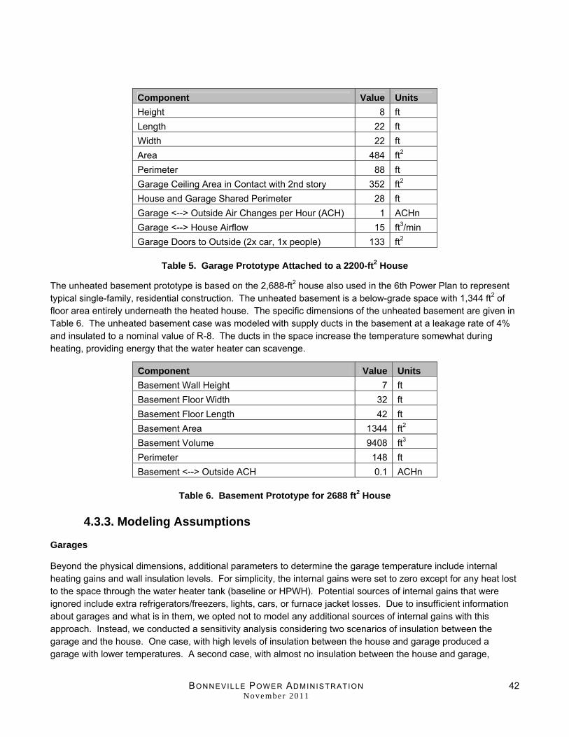
BONNEVILLE POWER ADMINISTRATION November 2011
42
Component Value Units
Height 8 ft
Length 22 ft
Width 22 ft
Area 484 ft2
Perimeter 88 ft
Garage Ceiling Area in Contact with 2nd story 352 ft2
House and Garage Shared Perimeter 28 ft
Garage <--> Outside Air Changes per Hour (ACH) 1 ACHn
Garage <--> House Airflow 15 ft3/min
Garage Doors to Outside (2x car, 1x people) 133 ft2
Table 5. Garage Prototype Attached to a 2200-ft2 House
The unheated basement prototype is based on the 2,688-ft2 house also used in the 6th Power Plan to represent typical single-family, residential construction. The unheated basement is a below-grade space with 1,344 ft2 of floor area entirely underneath the heated house. The specific dimensions of the unheated basement are given in Table 6. The unheated basement case was modeled with supply ducts in the basement at a leakage rate of 4% and insulated to a nominal value of R-8. The ducts in the space increase the temperature somewhat during heating, providing energy that the water heater can scavenge.
Component Value Units
Basement Wall Height 7 ft
Basement Floor Width 32 ft
Basement Floor Length 42 ft
Basement Area 1344 ft2
Basement Volume 9408 ft3
Perimeter 148 ft
Basement <--> Outside ACH 0.1 ACHn
Table 6. Basement Prototype for 2688 ft2 House
4.3.3. Modeling Assumptions
Garages
Beyond the physical dimensions, additional parameters to determine the garage temperature include internal heating gains and wall insulation levels. For simplicity, the internal gains were set to zero except for any heat lost to the space through the water heater tank (baseline or HPWH). Potential sources of internal gains that were ignored include extra refrigerators/freezers, lights, cars, or furnace jacket losses. Due to insufficient information about garages and what is in them, we opted not to model any additional sources of internal gains with this approach. Instead, we conducted a sensitivity analysis considering two scenarios of insulation between the garage and the house. One case, with high levels of insulation between the house and garage produced a garage with lower temperatures. A second case, with almost no insulation between the house and garage,

BONNEVILLE POWER ADMINISTRATION November 2011
43
produced warmer temperatures, which more closely tracked measured field data. Table 7 shows the nominal insulation values and total conductances used to develop the garage prototype and the associated temperature profile.
Garage-to-Outside Heat Transfers
Area (ft2)
R-Value (nominal) Btu/hr-F
Garage->Outside Exposed Perimeter 60 2 30.0
Garage->Outside Exposed Wall Area 347 19 18.3
Garage Doors 133 2 66.5
Garage->Attic Exposed Ceiling Area 132 30 4.4
Total Garage<-->Outside Conductance 119.2
Garage-to-House Interzone Heat Transfers
Insulated Walls between
House & Garage
Uninsulated Walls between
House & Garage
Area (ft2)
R-Value (nominal) Btu/hr-F
R-Value (nominal) Btu/hr-F
Garage->House Shared Wall Area 224 19 11.8 5 44.8
Garage->House Ceiling 352 30 11.7 7 50.3
Garage->House Airflow 16.2 16.2
Total Garage<-->House Conductance 39.7 111.3
Table 7. Garage Heat Transfer Conductances
Overall, the approach of low insulation and low internal gains is a conservative one because it more closely couples the house to the garage. Being more closely coupled, the house supplies more heat to the garage, amplifying heating system response to perturbations in garage temperature. Other scenarios, involving more sources of internal gains to the garage, could be imagined that would produce a similar temperature profile but have different impacts on the space heating system.
The modeled temperature profiles were compared to the EPRI field-measured profiles. Given the uncertainties in the modeling, however, the matching was performed in a non-rigorous fashion. In the field sites, there were eight garage installations in the Seattle area and nine garage installations in the Portland area. This type of installation and climate provides enough data to show the variation of temperature by site and forms the basis for comparison to modeled data.
Figure 27 shows the metered and modeled temperatures for Seattle. Outside temperatures, shown in blue, for the field data come from weather stations near the sites. The eight sites exhibit a considerable range of garage temperatures. The daily average of the eight is shown as a tick mark in the middle of the vertical red lines. Importantly, the metered data are not weather normalized and cover only four months of the year. Further, “normalizing” the garage temperatures is an ambiguous process that itself would require some sort of thermal model. For comparison, the modeled data also show four months of output but are based on “typical” weather from the TMY data sets. Differences in weather data preclude direct comparisons, but the “unins garage” (uninsulated boundary between house and garage) shows adequate agreement between modeled and measured temperatures.
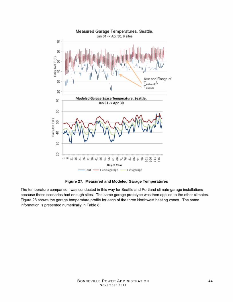
BONNEVILLE POWER ADMINISTRATION November 2011
44
Figure 27. Measured and Modeled Garage Temperatures
The temperature comparison was conducted in this way for Seattle and Portland climate garage installations because those scenarios had enough sites. The same garage prototype was then applied to the other climates. Figure 28 shows the garage temperature profile for each of the three Northwest heating zones. The same information is presented numerically in Table 8.

BONNEVILLE POWER ADMINISTRATION November 2011
45
Figure 28. Garage Annual Temperature Profiles
Unheated Basements
For unheated basements, there are fewer field sites, so far less is known about the model temperature calibration. Nonetheless, it stands to reason that the basement profile, with its extensive ground contact, should be fairly constant and smooth, especially with respect to the outside and garage. The temperature profile for the basement bears this out, showing temperatures above outside temperatures in the winter and below in the summer. Figure 29 shows the unheated basement temperature profile. The same information is presented numerically in Table 8.
Figure 29. Unheated Basement Annual Temperature Profiles

BONNEVILLE POWER ADMINISTRATION November 2011
46
Fraction of time per year in a given temperature bin
Garage Unheated Basement Temperature
bins (center)
HZ1 HZ2 HZ3 HZ1 HZ2 HZ3
77 0.006 0.004 0.000 0.000 0.000 0.000
72 0.049 0.086 0.049 0.009 0.006 0.000
67 0.110 0.134 0.093 0.055 0.074 0.016
62 0.208 0.131 0.137 0.265 0.193 0.181
57 0.148 0.105 0.140 0.294 0.226 0.181
52 0.251 0.156 0.121 0.300 0.195 0.211
47 0.161 0.190 0.200 0.067 0.252 0.214
42 0.055 0.132 0.167 0.009 0.053 0.197
37 0.010 0.045 0.071 0.000 0.000 0.000
32 0.002 0.015 0.019 0.000 0.000 0.000
27 0.000 0.000 0.003 0.000 0.000 0.000
Table 8. Buffer Space Temperature Profiles
The temperature bins were created based on daily average temperatures. Water heaters operate on hourly and sub-hourly time scales, so it may be appropriate for future work to consider creating profiles on an hourly basis.
4.4. COP Mapping
The bin method requires establishing an equipment COP for each temperature. For integrated heat pump water heaters, with two heating methods, the COP is determined not only by how efficiently the compressor operates at a given temperature but also by how much the resistance elements are used. The lower efficiency resistance elements always pull the COP down toward baseline levels.
The lab results from the COP test series characterize the compressor behavior well. They show the lower and upper temperature limits for compressor operation. Outside of these limits, the resistance element will provide all of the heat to the water, essentially setting the COP at 1.8 For equipment operating in compressor-only mode at temperatures within the operational envelope, the COP is calculated according to the curve fits presented in section 3.5. For equipment operating in mixed modes, with both resistance element and compressor operation, the COP becomes highly dependent on the user’s draw pattern and the tank control strategy response. Light usage patterns, relative to the storage capacity of the tank, allow the compressor to meet more of the water heating load. Heavy usage patterns often trigger the resistance elements, causing the system COP to drop. Moreover, higher output capacity compressors are more likely to be able to respond to heating demands without the need for supplemental resistance heat.
The compressor COP data from the lab are well defined, and so, for developing a whole-system operational COP map, the key quantity to resolve is the fraction of time the HPWH spends using resistance heating. The 1-hour, 24-hour, and DP-2 lab tests give insight into how the equipment will use resistance heating in response to different loads, but there is a larger variation in draw patterns from household to household than can be captured in the lab testing. In fact, the current, standard 24-hour draw profile, which is largely acknowledged as being unrepresentative, is being reviewed by DOE and the American Society of Heating, Refrigeration and Air
8 Technically, the DOE and ASHRAE test standards assign an efficiency of 0.98 to resistance heating elements (ASHRAE Std 118.2-2006; 10 CFR 430, 1998)

BONNEVILLE POWER ADMINISTRATION November 2011
47
Conditioning Engineers (ASHRAE) Standards Committee118.2 to be updated to a more representative pattern. To broaden the analysis, Ecotope binned the field-observed daily input and output by equipment model and temperature. By examining the daily energy input and evaluating it based on what is expected from compressor use only, it is possible to determine the resistance heat runtime. The runtime and combined system COP were then further compared against documented lab observations from the operating mode and draw profile type tests. Taken together, the approach creates the COP map needed in the bin analysis.
Table 9 shows calculations at one set of ambient conditions where overall usage has been parsed into compressor and resistance element operation accordingly. The table demonstrates the severe reduction on COP imposed by switching to resistance heat, even for short amounts of time. Calculations are conducted for a daily water use of 49 gallons. Compressor COP, power, and output are averages based on heating water from 90°F and 120°F. Heat extracted is the energy extracted from the ambient environment by the heat pump net of standby losses.
Voltex GeoSpring EcoSense
Compressor COP 2.8 3.0 2.8
Compressor Runtime (min) 240 312 84
Resistance Element Runtime (min) 5 36 84
Compressor Output (kBtu) 33.6 25.3 13.1
Resistance Output (kBtu) 1.2 9.0 23.4
%Output provided by resistance elements 3% 26% 64%
%Input drawn by resistance elements 9% 52% 84%
System COP, no standby losses 2.6 1.9 1.3
System COP, with standby losses 2.3 1.7 1.1
Heat extracted (kBtu) 17.2 12.8 2.3
Units of measure: min = minutes; kBtu = kilo British thermal units
Table 9. HPWH daily input/output specifications at 67°F and 50% RH
Figure 30 shows the COP map developed with the lab and field data. The COPs for the GeoSpring and the EcoSense are smoothed with a linear fit for the data between 52°F and 77°F. Data for the Voltex at temperatures above 57°F were not encountered in the partial year field data set, so COPs beyond that temperature are predicted assuming resistance element runtime equivalent to the 57°F point. Lastly, the baseline resistance heating tank COPs are based entirely on calculations using the baseline tank heat loss rate and daily water usage (see section 4.2).

BONNEVILLE POWER ADMINISTRATION November 2011
48
Figure 30. COP Map
Of note in Figure 30 is the COP at low ambient temperatures. At cold temperatures where the compressor does not run, the COP of the HPWHs is often below the COP of the baseline tank. This indicates that the HPWHs tested lose heat more rapidly to their surroundings than a traditional water heater.9 For the EcoSense, the drop in COP below the baseline is noticeably larger. In addition to reduced insulation, the lab findings show that the EcoSense circulation pump sometimes runs even without the compressor. The effect is twofold. First, the pump consumes energy while running that is not added to the water, increasing power draw while leaving tank energy unaltered. Second, drawing the water into a circulation pipe outside of the tank increases heat loss to the surroundings.
Figure 30 shows a temperature range from about 45°F to 60°F where the performance regime transitions from resistance element operation at colder temperatures to mainly compressor operation at warmer temperatures. The transition is most abrupt for the Voltex, while the GeoSpring transition occurs more slowly over a wider range. The compressor cutoff for both models is near 45°F, with the lab tests showing the Voltex able to operate at slightly colder air and water temperatures. Near this cutoff temperature, large water draws drive the tank temperature down and, in turn, the refrigerant temperature, causing the compressor to cycle off to avoid coil frosting. In that case, the resistance elements engage to provide heat.
Lab findings showed the EcoSense compressor to cease functioning between 57°F and 67°F, which readily explains the low observed COPs in the field data for temperatures of 65°F and below. One possible explanation for the low COPs above 60°F could be that the occupants selected hotter setpoints or less efficient operating modes to compensate for reductions in hot water availability due to tank destratification.
9 The two 50-gallon tanks are less insulated than the 50-gallon baseline tank. The 80-gallon Voltex shows a higher heat loss rate than the baseline 50-gallon tank used across this analysis, but it has comparable insulation to an 80-gallon resistance tank.

BONNEVILLE POWER ADMINISTRATION November 2011
49
Lastly, the COP map shows, at least implicitly, the differing control strategies: how quickly the HPWH switches from compressor to resistance element. As elucidated in section 3.4.1, under heavy usage the EcoSense is quickest to activate resistance heat, followed by the GeoSpring, followed by the Voltex. This trend is borne out in the COP map, showing that a hesitancy to activate resistance elements leads to dramatically higher observed COPs.
4.5. Garage, Unheated Basement, and Interior Energy Use
The total amount of energy added to the water throughout the year can be calculated as:
DHWyrly = GPD * ρwater * cp water * ΔT * 365 days/year
where GPD is daily water volume, ρwater is the density of water, cp water is the heat capacity of water, and ΔT is the inlet-outlet water temperature rise. This represents a situation where there are no standby losses and the heating efficiency is unity. Using the baseline water inputs and a COP of 1, DHWyrly is 3111kWh/yr (10615 kBtu/yr). To calculate the effect of different tank heating efficiencies and standby losses, we divide DHWyrly by the annualized COP.
The annualized COP is determined by applying the COP map to the temperature bin profile for each installation location and climate zone. The estimated COP and associated energy use are shown in Table 10. The table shows the energy use for the water heater only and does not account for the interaction with the house. Further, the temperature profile for the conditioned space asserts a constant, year-round temperature of 67°F.
Annual COP Annual Energy Use (kWh) Installation Location
Model HZ1 HZ2 HZ3 HZ1 HZ2 HZ3
Voltex 1.9 1.8 1.4 1616 1720 2168
GeoSpring 1.3 1.3 1.1 2346 2458 2883
EcoSense 0.9 0.8 0.8 3614 3671 3988 Garage
Baseline 0.9 0.9 0.9 3475 3484 3529
Voltex 2.0 1.9 1.7 1545 1663 1809
GeoSpring 1.4 1.3 1.2 2282 2463 2646
EcoSense 0.9 0.8 0.8 3626 3720 3858
Unheated Basement
Baseline 0.9 0.9 0.9 3473 3483 3495
Voltex 2.3 1359
GeoSpring 1.7 1846
EcoSense 1.0 3002
Conditioned Space
Baseline 0.9 3424
Table 10. Annual COP and Energy Use Estimates (HPWH only)

BONNEVILLE POWER ADMINISTRATION November 2011
50
4.6. Heating and Cooling System Interactions
4.6.1. Overview and Qualitative Discussion
The very nature of heat pump operation requires HPWHs to extract heat from whatever space they occupy. An air-source heat pump installed outdoors extracts heat from a plentiful source—the outside air—and so does not noticeably change the temperature of the heat source. Further, the heat extracted from the atmosphere in this way is generally considered free energy, thereby creating COPs greater than 1. An HPWH installed in spaces enclosed by a house, either in a buffer space or the interior, becomes coupled to the house heating and cooling system. The heat extracted by the HPWH could have been useful to the house in maintaining the setpoint during the heating season. Conversely, in the cooling season, heat extracted from the house could be counted towards a cooling benefit. Accounting for the heating debits and cooling credits is instrumental in determining the total energy impact of HPWH installations.
The energy interaction with the house varies with tank characteristics and the operating environment. First, greater use of the resistance element extracts less heat from the space. Second, by definition, the higher the heat pump COP, the more heat is extracted. The COP changes with ambient temperature, with warmer temperatures leading to greater heat removal. Conversely, lower temperatures lead to lower COPs and less heat removal. Third, compressor size changes the energy impact with larger capacities extracting more heat. Lastly, common to all water heating tanks, standby losses add heat back to the space. In an interesting twist, the standby losses warm the space where the HPWH is located, providing heat that can be harvested by the HPWH.10
The energy interaction further depends on where the water heater is located: buffer spaces like garages and unheated basements, or inside conditioned space. Interior installations clearly have a direct impact on the house heating and cooling load. Buffer space installations have an indirect impact caused by a decrease in the buffer space temperature and an increase in heat loss from the house, consequently increasing the heating load. In other words, the house heating system, in the absence of the HPWH, sees a load that depends on the buffer space being at a certain temperature. Operating an HPWH in that buffer space changes the temperature and hence the heating load. The overall impact greatly depends on how closely the buffer space is thermally coupled to the house. For example, lower insulation levels between the house and buffer space lead to greater interactive effects. Additionally, ducts placed in an unheated basement more closely couple the buffer to the house via duct leakage and conduction effects. Other sources of heat for the buffer spaces that do not come from the house include ground contact, solar gains, and natural outside air infiltration. Those sources can largely be considered forms of “free” energy.
Although the energy flows are the same, the heating, cooling, and cost implications depend on the heating, ventilation, and air conditioning (HVAC) system installed in the house. The impacts are most directly considered for interior installations. For example, for houses with gas furnaces, the source of some of the heat extracted by the HPWH is provided by natural gas, indirectly creating, in effect, a hybrid fuel water heater (the HPWH removes energy from the air that is replaced with energy from the gas furnace). In this scenario, the annual electric usage decreases but the gas usage increases. Next, for houses with electric resistance heat, the energy to heat the water in the heating season will be supplied with a COP of 1. This will create, in effect, an all-electric resistance
10 Interestingly, for the equipment in this study, at 67°F ambient temperature, the standby losses and heat extracted from the space are approximately equal with about 4-5gallons of water used per day, so that the HPWH has no net impact on ambient space temperature.

BONNEVILLE POWER ADMINISTRATION November 2011
51
water heating system for part of the year, resulting in no difference from the baseline case. Houses with heat pump space heat will see an increase in space heating kWh usage, but the impact will be far less than in resistance-heated homes. The space heating heat pump, combined with the HPWH, effectively creates a two-stage compressor system to heat the water. In the winter, when both compressors are running, the efficiency with which the water is heated ultimately depends on the efficiency of both compressors. For buffered space installations, all the same concepts apply, except that the interaction with the building’s space heating system is far less.
4.6.2. Modeling the Interactions
Clearly, the HPWH and space conditioning systems interact in dynamic and complicated ways. To fully model the interactive system requires simulation tools which do not yet exist. Instead, the modeling is conducted with existing tools adapted in ways to make them as representative as possible of the interactive effects. The underlying concept is to account for HPWH space heating effects with negative or reduced internal gains, applied to the space in which the unit is installed.
As with determining the annual temperature profiles, SUNCODE was used to model garage installations while SEEM was used to model unheated basement and interior installations. For each installation location, two simulations were performed, differing only in the level of internal gains, and compared to determine the net energy impact on the space conditioning system.
The simulations allow only a constant hourly internal gains schedule over the course of the day. Tank water heaters do not run on a constant basis but rather have several on/off periods throughout the day. The constant hourly schedule misses that effect but does capture the total daily heat extracted.11 In an attempt to capture some of the effect of changing COP with temperature, the simulations for the buffer spaces use a seasonal schedule to change the heat extracted per day. The heat impact roughly corresponds to temperature regimes of 47°F, 57°F, and 67°F and COPs from a “generic” HPWH model (combination of the Voltex and GeoSpring water heaters). The three COPs were used to correspond to garage temperatures seasonally.12 The buffer space internal gains were modeled with a generic, composite water heater and not specific equipment to reduce the simulation complexity.
As alluded to in the qualitative discussion of the HPWH interaction, the impact on the HVAC system will depend on the distribution and system efficiency. More efficient HVAC equipment and delivery systems decrease the impact of the water heater. The scenarios considered in this analysis include zonal resistance heat, a gas furnace with Annual Fuel Utilization Efficiency (AFUE) 90, and a heat pump with a heating season performance factor (HSPF) of 8.5. The scenarios also included ducts meeting the Performance Tested Comfort Specification standards for leakage and insulation with delivery efficiency approximately 90% (RTF 2011b). The somewhat higher efficiencies were selected so that the analysis could reflect HPWH installations on a “last measure in” basis. Equipment and delivery systems with lower efficiencies will increase the magnitude of the space heating interaction. All cooling is modeled with a seasonal energy efficiency ratio (SEER) 13 air conditioner.
11 For instance, the total amount of heat extracted per day for an HPWH installed in a conditioned space at 67°F is given in Table 9. A total of 12.8 kBtu/day translates to a reduction in internal gains equivalent to 533 Btu/hr. All of the conditioned space scenarios used the levels of heat extracted given in Table 9. 12 The daily internal gains change by season as follows, with all values expressed in heat removed: from October to March they are 210 Btu/hr; from April to June they are 380 Btu/hr; from July to September they are 540 Btu/hr.

BONNEVILLE POWER ADMINISTRATION November 2011
52
4.6.3. Space Heating interactions
Table 11 shows the heating and cooling impact outputs from the simulations for buffer spaces. Negative values indicate a debit (more energy is needed from the heating system), and positive numbers indicate a benefit (less energy needed in cooling). The table shows that, for garage installations, the HPWH harvests about 200kWh/yr from the house in heating (indicated by the zonal resistance case, which has system COP of 1). By comparison, the unheated basement case is coupled more closely to the house, resulting in greater heating interactions. The modeled garage air change rates are much higher than the basement, which contributes to its decoupling from the house. The cooling impacts for the buffer spaces are small and modeled only for the Northwest regional aggregate cooling zone. Finally, as mentioned earlier, the table gives the interactions only in terms of the “generic” HPWH. Specific equipment models would have slightly different interactions, although the differences are considerably narrowed due to the nature of buffer spaces.
Garage Installation Impacts by System Type
HVAC System Type Units HZ1 HZ2 HZ3
Zonal Resistance kWh/yr -184 -177 -203
Gas Furnace AFUE 90 therms/yr -8 -7 -9
Heat Pump HSPF 8.5 kWh/yr -81 -85 -104
Cooling SEER 13 kWh/yr 10
Unheated Basement Installation Impacts by System Type
HVAC System Type Units HZ1 HZ2 HZ3
Zonal Resistance kWh/yr -440 -467 -539
Gas Furnace AFUE 90 therms/yr -17 -18 -20
Heat Pump HSPF 8.5 kWh/yr -175 -203 -247
Cooling SEER 13 kWh/yr 75
Table 11. Annual Space Heating Impacts, Buffer Space Installations
Table 12 displays the simulated heating and cooling impacts for interior space installations. Overall, as is expected, the magnitudes are larger than for the buffer spaces. In contrast to the buffer space simulations, the three HPWH models are simulated separately for interior installations. The output shows a large variation in impacts, which is caused by differences in system COP at room temperature conditions, itself caused primarily by differing operational strategies. Once again, the fraction of heat provided by the compressor vs. resistance elements greatly affects the results. Equipment operating with more compressor usage and higher COP extracts more heat from the ambient environment, creating a larger heating debit or cooling credit.

BONNEVILLE POWER ADMINISTRATION November 2011
53
Conditioned Space Impacts
HVAC Type HPWH Units HZ1 HZ2 HZ3
Voltex -1114 -1139 -1223
GeoSpring -823 -845 -907 Zonal
Resistance EcoSense
kWh/yr
-143 -148 -159
Voltex -52 -52 -57
GeoSpring -39 -39 -42 Gas
Furnace AFUE 90
EcoSense
therms/yr
-7 -7 -7
Voltex -365 -472 -622
GeoSpring -269 -347 -459 Heat Pump HSPF 8.5
EcoSense
kWh/yr
-46 -60 -80
Voltex 121
GeoSpring 91 Cooling
SEER 13 EcoSense
kWh/yr
17
Table 12. Annual Space Heating Impacts, Conditioned Space Installations
4.7. Energy Savings Estimates
The final energy savings estimates, which account for the annual water heater COP and the interaction of the heating and cooling system, are found by combining the information in Table 10, Table 11, and Table 12. The energy use of the water heater and the interactive effects are additive. HVAC systems with cooling—for example, a gas furnace with air conditioning or heat pump—include the benefit of added cooling from the HPWH. The overall savings estimates are presented in graphs in Figure 31, Figure 32, and Figure 33. For gas-heated houses, there are always two sets of numbers needed to track the change in both electricity and gas usage. It is interesting to observe that the savings estimates for unheated basement installations are less than those for garage installations, despite the annual COPs being comparable. The outcome is largely due to the basements being more closely coupled to the house in the modeling scenarios, incurring greater heating system penalties. Additionally, unheated basements don’t benefit from the higher air temperatures in the summer that the garages do.
The conditioned space installations exhibit dramatically different outcomes based on heating system type. First, the resistance-heated house shows the lowest savings because, during the heating season, energy extracted by the HPWH is regained with a COP of 1. In this scenario, the HPWH functions much as a resistance heater would, because the heat is generated with zonal electric resistance, and then the compressor draws energy transferring that heat into the tank. In general, differences in HPWH COP cause only subtle differences in wintertime savings. The space heating system initially generating the heat bears much more heavily on the overall impact of the HPWH. It is only during the shoulder and hotter seasons where the heat source is “free energy” from the outside air or solar gains that the different COPs show up with different savings levels. Gas-heated houses show the most electric savings, but at the expense of increased therm consumption. Heat-pump houses predictably show the highest level of total energy savings. The heat pump providing heat to the house decreases the overall energy cost of the HPWH extracting that heat to add to the water.

BONNEVILLE POWER ADMINISTRATION November 2011
54
Figure 31. Annual Energy Savings with Gas Furnace

BONNEVILLE POWER ADMINISTRATION November 2011
55
Figure 32. Annual Energy Savings with Zonal Resistance Heat
Figure 33. Annual Energy Savings with Heat Pump

BONNEVILLE POWER ADMINISTRATION November 2011
56
4.8. RTF Energy Use and Savings Estimates
At the time of this writing, the RTF13 is pursuing a provisional “unit energy savings” estimate for HPWHs. The approach is based on the same methods detailed in this report; however, the RTF is attempting to incorporate other emerging HPWH models into the savings estimate framework and anticipate future models coming to market over the next two to three years. The approach will likely produce different savings estimates than those in this report, potentially based on a combination of models to create different product categories and/or daily draw volumes. The proposed approach is currently in flux and expected to change further. As such, it is not compared to this analysis. Any differences will likely be slight changes to input assumptions or result from aggregating water heater models into different categories.
13 http://www.nwcouncil.org/energy/rtf/Default.htm

BONNEVILLE POWER ADMINISTRATION November 2011
57
5. Conclusions
5.1. Lessons Learned Throughout the course of the project, including during final report writing, several key features of the way the project was conducted (a/k/a “lessons learned”) proved worthy of mention:
Convening an advisory committee of HPWH stakeholders proved helpful in developing a measurement plan that could address concerns across the region.
The comprehensive test plan, applied in the same way across all equipment evaluated, was useful in achieving consistent testing and results.
Working with an experienced and capable lab was crucial to developing reliable data. Moreover, NREL provide additional expert insight that improved the overall project quality.
The operating mode tests may be somewhat redundant, because the exact same information is inescapably gathered throughout the other tests. The value of the operating mode tests appears to be helping the lab personnel familiarize themselves with the equipment and rigorously observing the non-default operating modes.
Draw profile DP-2, with its four consecutive showers, proved highly enlightening. This suggests that future studies should include a dedicated shower test—the number of consecutive, comfortable showers available from a given water heater. As a measurement of output capacity, this would be highly relevant, practical, and easy to understand. It would also greatly inform water heater response to high-demand situations.
Translating the lab results to real-world installations proves challenging due to the sheer diversity of draw patterns. Building on the insight gained from DP-2, it would be useful to develop a suite of prototypical draw patterns to run in the lab that are more representative of actual hot water usage profiles. Potentially, a set of three draw patterns could be tested: small, medium, and large. The results could be used independently to apply to different loads or could be weighted together to give a generalized picture of the water heater behavior.
Modeling the HPWH interactions with residential buildings is a complicated task. It would benefit from further refinements in the future. New modeling tools could be developed to fully integrate HPWH equipment operation and placement with annual energy use simulations. The tools would more accurately capture the dynamic interactions between the water heater and the building.
5.2. Equipment Design and Operation
The design considerations that appear most relevant for HPWH installations in the Northwest are tank capacity, low-temperature compressor operation, compressor output capacity, and configuring control strategies to minimize the use of resistance elements. Large tank capacity, relative to the hot water load, is a general requirement for any effective HPWH, necessary to make full use of heat pump efficiency. Smaller tanks can switch more quickly to resistance heating during periods of high demand, discarding the potential efficiency advantages of the heat pump, so large storage capacity is required to dissuade resistance element activation.

BONNEVILLE POWER ADMINISTRATION November 2011
58
Likewise, the control strategy, even for a larger-sized tank, needs to be configured to activate the resistance elements only when they are needed and not before.
Low-temperature compressor operation is a concern more specific to the Northwest region, as units installed in buffer spaces, such as garages, experience cooler ambient temperatures much of the year. Successful compressor operation at these low ambient temperatures is crucial to justify the upgrade to an HPWH. Otherwise, the unit functions more like an elaborate and expensive electric resistance water heater. Further, adequately sized compressors are necessary to expedite the efficient recovery of the tank, decreasing the need for resistance heating. The larger compressor capacity, coupled with a larger evaporator coil, also helps to retain output at low temperatures.
5.3. Installation Location Findings
The energy use savings estimates predict a wide range of outcomes based on equipment model, installation location, climate zone, and house heating system type. Not surprisingly, buffer spaces show the least dependence on the heating system type but the largest on the climate zone. Because of the lower temperatures in buffer spaces in the colder climates, the performance of the equipment selected is impacted more decisively by the climate zone. The propensity of certain models to engage the resistance heating elements becomes even more evident given ambient temperature swings typical of colder conditions. Differences in the type of buffer space—garage or unheated basement—are smaller than those due to climate zone or equipment model.
Predicted conditioned space installations show dependencies in decreasing levels of importance on three factors: house heating system, equipment model, and climate zone. The results show that, for interior installations, savings depend critically on the heating system type. Houses with heat pump heating demonstrate the largest energy savings, while the other system types offer some level of savings but also require a large tradeoff by obtaining considerable water heating energy from the HVAC system.
It should be pointed out that all the predicted savings estimates are predicated on simulations and the specific model inputs that drive the simulations. The analysis has attempted to choose reasonable inputs in order to illustrate the interactive effects and enable energy use calculations. Other scenarios, with different model assumptions, could be imagined that would produce different outputs. Nevertheless, the HPWH and house HVAC components form a coupled system that can’t be neglected. For example, if the model inputs are adjusted in a way as to more closely couple the buffer space to the house, the buffer space temperatures will increase. Although the HPWH COP would increase accordingly, the amount of energy harvested from the house would increase as well. The interactions are nonlinear, making quantifiable adjustments challenging. Qualitatively, however, changes to the modeling inputs often produce system outputs that work in opposing directions. The energy changes do not necessarily cancel, but their effects are reduced.
Overall, the project demonstrated estimated energy consumptions showing that HPWHs can be a viable source of energy savings. The savings can vary considerably based on the equipment, installation location, and climate. Still, there are a number of combinations that will likely lead to reduced energy usage over a traditional resistance-only hot water tank.

BONNEVILLE POWER ADMINISTRATION November 2011
59
References
[10 CFR 430] U.S. Department of Energy, Office of Energy Efficiency and Renewable Energy. “Energy Conservation Program for Consumer Products: Energy Conservation Standards for Water Heaters; Final Rule.” Federal Register, 66 FR 4474, January 17, 2001 http://www1.eere.energy.gov/buildings/appliance_standards/residential/pdfs/water_heater_fr.pdf
[10 CFR 430] U.S. Department of Energy, Office of Energy Efficiency and Renewable Energy. “Energy Conservation Program for Consumer Products: Appendix E to Subpart B of Part 430—Uniform Test Method for Measuring the Energy Consumption of Water Heaters.” Federal Register, 63 FR 25996, May 11, 1998, pp. 26008-26016. http://www1.eere.energy.gov/buildings/appliance_standards/residential/pdfs/wtrhtr.pdf
ASHRAE Standard 118.2-2006. “Method of Testing for Rating Residential Water Heaters.” American Society of Heating, Refrigeration and Air Conditioning Engineers, Atlanta, GA. 2006.
ASHRAE, 2009, “Handbook of Fundamentals,” American Society of Heating, Refrigeration and Air Conditioning Engineers, Atlanta, GA.
Hanford, Jim, Mike Kennedy, Mary Jane DeLaHunt, and Larry Palmiter, 1985. Heat Pump Water Heater Field Test. Ecotope Inc. June 1985. Prepared for the Bonneville Power Administration.
NPCC, 2010. Sixth Northwest Conservation and Electric Power Plan. Northwest Power and Conservation Council. February 2010. http://www.nwcouncil.org/energy/powerplan/6/default.htm
Quaid, Maureen, Rick Kunkle and Brian Lagerberg, 1991. RCDP 2 Appliance Analysis, Washington State Energy Office, August 1991.
Roos, Carolyn and David Baylon, 1993. Non-Space Heating Electrical Consumption in Manufactured Homes RCDP Cycle II. Ecotope Inc. May 1993.
RTF, 2011a. "RTF Deemed Measures: Residential: DHW - Efficient Tanks." Northwest Power and Conservation Council. Regional Technical Forum, 2011. http://www.nwcouncil.org/energy/rtf/measures/measure.asp?id=125
RTF, 2011b. "RTF Deemed Measures: Residential: Heating/Cooling - PTCS Duct Sealing SF." Northwest Power and Conservation Council. Regional Technical Forum, 2011. http://www.nwcouncil.org/energy/rtf/measures/measure.asp?id=138

BONNEVILLE POWER ADMINISTRATION November 2011
60
Appendix A. Instrumentation List List of sensors used in laboratory testing
Measurement Unit Sensor Type Accuracy
Temperature
Inlet Air Dry Bulb °C T-type Thermocouple ArrayGreater of: ±0.5°C or 0.4% reading
Outlet Air Dry Bulb °C T-type Thermocouple ArrayGreater of: ±0.5°C or 0.4% reading
Inlet Water °C T-type Insertion Thermocouple
Greater of: ±0.5°C or 0.4% reading
Outlet Water °C T-type Insertion Thermocouple
Greater of: ±0.5°C or 0.4% reading
Tank Internal Temperatures 1-6 °C 1/16”, ungrounded T-type Thermocouple
Greater of: ±0.5°C or 0.4% reading
Evaporator Temperature - Refrigerant Inlet
°C T-type Surface-Mounted Thermocouple
Greater of: ±0.5°C or 0.4% reading
Evaporator Temperature - Refrigerant Outlet
°C T-type Surface-Mounted Thermocouple
Greater of: ±0.5°C or 0.4% reading
Evaporator Temperature - Saturation
°C T-type Surface-Mounted Thermocouple
Greater of: ±0.5°C or 0.4% reading
Evaporator Temperature - Saturated Discharge
°C T-type Surface-Mounted Thermocouple
Greater of: ±0.5°C or 0.4% reading
Pressure
Ambient Air Pa Pressure Transducer ±4 Pa Inlet Air Pa Pressure Transducer ±4 Pa Outlet Air Pa Pressure Transducer ±4 Pa Water (tank inlet) Pa Pressure Transducer ±0.25% of reading Humidity
Ambient Air Dew Point °C Chilled Mirror Hygrometer ±0.2°C Inlet Air Dew Point °C Chilled Mirror Hygrometer ±0.2°C Outlet Air Dew Point °C Chilled Mirror Hygrometer ±0.2°C
Power
Test Article Power Watts Watt Node ±25 W Compressor Power (GE, AOS) Watts Watt Node ±15 W Compressor Power (Rheem) Watts Watt Node ±0.2% of reading Fan Power (Rheem, AOS) Watts Watt Node ±0.2% of reading Fan Power (GE) Watts Watt Node ±2 W Pump Power (Rheem) Watts Watt Node ±0.2% of reading
Resistance Element Power Watts Calculated from other power measurements
Flow
Inlet Air kg/s Calculated using laboratory equipment (nozzle box)
±1.5% of reading
Outlet Air kg/s Calculated using laboratory equipment (LFE)
±2.0% of reading
Inlet Water kg/s Turbine Flow meter ±1.5% of reading Outlet Water kg/s Turbine Flow meter ±1.5% of reading

BONNEVILLE POWER ADMINISTRATION November 2011
61
Condensate kg/s Coriolis Flow meter ±0.1% of reading

BONNEVILLE POWER ADMINISTRATION November 2011
62
Appendix B. Graphs
B 1. AO Smith Voltex COP47 Test ............................................................................................................. 64
B 2. GE GeoSpring COP47 Test ................................................................................................................ 64
B 3. Rheem EcoSense COP47 Test .......................................................................................................... 65
B 4. AO Smith Voltex COP57 Test ............................................................................................................. 65
B 5. GE GeoSpring COP57 Test ................................................................................................................ 66
B 6. Rheem EcoSense COP57 Test .......................................................................................................... 66
B 7. AO Smith Voltex COP67 Test ............................................................................................................. 67
B 8. GE GeoSpring COP67 Test ................................................................................................................ 67
B 9. Rheem EcoSense COP67 Test .......................................................................................................... 68
B 10. AO Smith Voltex COP77 Test ........................................................................................................... 68
B 11. GE GeoSpring COP77 Test .............................................................................................................. 69
B 12. Rheem EcoSense COP77 Test ........................................................................................................ 69
B 13. AO Smith Voltex COP85 Test ........................................................................................................... 70
B 14. GE GeoSpring COP85 Test .............................................................................................................. 70
B 15. Rheem EcoSense COP85 Test ........................................................................................................ 71
B 16. AO Smith Voltex COP95 Test ........................................................................................................... 71
B 17. GE GeoSpring COP95 Test .............................................................................................................. 72
B 18. Rheem EcoSense COP95 Test ........................................................................................................ 72
B 19. AO Smith Voltex COP95 Dry Test .................................................................................................... 73
B 20. GE GeoSpring COP95 Dry Test ....................................................................................................... 73
B 21. Rheem EcoSense COP95 Dry Test.................................................................................................. 74
B 22. AO Smith Voltex COP105 Test ......................................................................................................... 74
B 23. GE GeoSpring COP105 Test ............................................................................................................ 75
B 24. Rheem EcoSense COP105 Test ...................................................................................................... 75
B 25. AO Smith Voltex COP105 Dry Test .................................................................................................. 76
B 26. GE GeoSpring COP105 Dry Test ..................................................................................................... 76
B 27. Rheem EcoSense COP105 Dry Test................................................................................................ 77
B 28. AO Smith Voltex DP-2, Full Test....................................................................................................... 77
B 29. GE GeoSpring DP-2, Full Test.......................................................................................................... 78
B 30. Rheem EcoSense DP2, Full Test ..................................................................................................... 78
B 31. AO Smith Voltex DP3........................................................................................................................ 79
B 32. GE GeoSpring DP3........................................................................................................................... 79
B 33. Rheem EcoSense DP3 ..................................................................................................................... 80

BONNEVILLE POWER ADMINISTRATION November 2011
63

BONNEVILLE POWER ADMINISTRATION November 2011
64
COP Test Results, All
B 1. AO Smith Voltex COP47 Test
B 2. GE GeoSpring COP47 Test

BONNEVILLE POWER ADMINISTRATION November 2011
65
B 3. Rheem EcoSense COP47 Test
B 4. AO Smith Voltex COP57 Test

BONNEVILLE POWER ADMINISTRATION November 2011
66
B 5. GE GeoSpring COP57 Test
B 6. Rheem EcoSense COP57 Test

BONNEVILLE POWER ADMINISTRATION November 2011
67
B 7. AO Smith Voltex COP67 Test
B 8. GE GeoSpring COP67 Test

BONNEVILLE POWER ADMINISTRATION November 2011
68
B 9. Rheem EcoSense COP67 Test
B 10. AO Smith Voltex COP77 Test

BONNEVILLE POWER ADMINISTRATION November 2011
69
B 11. GE GeoSpring COP77 Test
B 12. Rheem EcoSense COP77 Test

BONNEVILLE POWER ADMINISTRATION November 2011
70
B 13. AO Smith Voltex COP85 Test
B 14. GE GeoSpring COP85 Test

BONNEVILLE POWER ADMINISTRATION November 2011
71
B 15. Rheem EcoSense COP85 Test
B 16. AO Smith Voltex COP95 Test

BONNEVILLE POWER ADMINISTRATION November 2011
72
B 17. GE GeoSpring COP95 Test
B 18. Rheem EcoSense COP95 Test

BONNEVILLE POWER ADMINISTRATION November 2011
73
B 19. AO Smith Voltex COP95 Dry Test
B 20. GE GeoSpring COP95 Dry Test

BONNEVILLE POWER ADMINISTRATION November 2011
74
B 21. Rheem EcoSense COP95 Dry Test
B 22. AO Smith Voltex COP105 Test

BONNEVILLE POWER ADMINISTRATION November 2011
75
B 23. GE GeoSpring COP105 Test
B 24. Rheem EcoSense COP105 Test

BONNEVILLE POWER ADMINISTRATION November 2011
76
B 25. AO Smith Voltex COP105 Dry Test
B 26. GE GeoSpring COP105 Dry Test

BONNEVILLE POWER ADMINISTRATION November 2011
77
B 27. Rheem EcoSense COP105 Dry Test
Draw Profile Tests
B 28. AO Smith Voltex DP-2, Full Test

BONNEVILLE POWER ADMINISTRATION November 2011
78
B 29. GE GeoSpring DP-2, Full Test
B 30. Rheem EcoSense DP2, Full Test

BONNEVILLE POWER ADMINISTRATION November 2011
79
B 31. AO Smith Voltex DP3
B 32. GE GeoSpring DP3

BONNEVILLE POWER ADMINISTRATION November 2011
80
B 33. Rheem EcoSense DP3