Reserves Augmentation by Designing an Optimum Waterflood Pattern with Black Oil Simulator

IOSR Journal of Mechanical and Civil Engineering (IOSRJMCE)

ISSN : 2278-1684 Volume 2, Issue 1 (July-August 2012), PP 62-77 www.iosrjournals.org

www.iosrjournals.org 62 | Page

Reserves Augmentation by Designing an Optimum Waterflood

Pattern with Black Oil Simulator

Osama Ikram

University of Engineering and Technology, Lahore, Pakistan

Abstract: In petroleum production system, reservoir pressure is considered to be main source of hydrocarbon

production from reservoir to the surface. With passage of producing time; fluids can only be lifted at the

economic rates from subsurface to the surface by some secondary recovery method which sweeps remaining oil

from the reservoir to improve its overall recovery.

Waterflooding is the dominant fluid injection technique and is frequently applied worldwide secondary

recovery process, which involves water injection in the oil formation under high pressure through an injection

well to enhance oil recovery of the well(s) of interest.

Selection of optimum number of wells and their optimum location is a whip hand to plan and

implement a successful waterflooding operation on a depleted reservoir to prevent the wastage of substantial capital investment. This involves efficacious and judicious selection of waterflooding pattern to augment the

reserves. This study emphasizes on importance and effect of efficiently selecting an optimum waterflood pattern

for primary production depleted reservoir “W” by simulating its performance for regular 5-spot & 9-spot

patterns to acquire, best technical & economic match for subject reservoir for a particular injectivity, reservoir

areal heterogeneity, direction of formation fractures, existing production wells and their spacing etc.

Where different opportunities involving a particular measurement or calculation are involved, there is

no substitute for thinking out the best solution to the problem. The mistakes should be made on paper where an

eraser can remove them, not in the field where someone must live with it.

I. Introduction Using computer modelling to simulate hydrocarbon reservoir behaviour and recovery performance

evaluation is an arduous task. The case study deals with developing a five spot and nine spot models on “Reservoir W” which is a solution gas-drive reservoir and its performance prediction using reservoir simulation.

The study also includes comparison and economic analysis of five spot and nine spot models.

The tasks included are:

1. Construct reservoir models for primary recovery five-spot and nine-spot waterflood patterns using Black

Oil simulator; ECLIPSE “E 100”1,2.

2. Run reservoir simulations for all models.

3. Perform economic calculations for all models.

4. Compare the economics and simulation results by Dec. 31, 2041 for recovery, water cut, average reservoir

pressure, oil production rate, gas-oil ratio, cumulative oil production, oil saturation, and pressure

distribution between 5-spot and 9-spot patterns.

II. Reservoir Description A conceptual petroleum production unit which is a solution gas-drive reservoir having anticlinal

structure with 20,000 ft*11,000 ft*65 ft in size is to be simulated. “Reservoir W” is a heterogeneous layered

reservoir with sandstone formation has an areal coverage of 5050.50 acres (20.439 km2) and bulk volume (Vb)

of 328,282.5 acre ft. The initial pressure of the reservoir is 3514.7 psia with solution GOR (Rsi) =450 SCF/STB

and its bubble point pressure is 1934.07 psia. The OOIP=2.23*108 STB. The formation compressibility is

approximately 6E-6 sip at Pb pressure and thickness of reservoir is 65 ft.

Basic model Setup

The unit is approximated into 100 * 55 regular grids in horizontal layers and each cell is 200 ft in

length; and 4 layers in the vertical direction (as 20 ft, 30 ft, 10 ft and 5 ft respectively) i.e. Model Dimensions :100x55x4 = 22,000

Grid Type : Cartesian

Geometry Type: Block centred

Grid Dimensions

Layer 1 : 100x55x (200)2x20 ft3

Layer 2 : 100x55x (200)2x30 ft

3

Layer 3 : 100x55x (200)2x10 ft3

Reserves Augmentation by Designing an Optimum Waterflood Pattern with Black Oil Simulator


Layer 4 : 100x55x (200)2x5 ft3

As the reservoir has an anticlinal structure so the grid top is not uniform. According to data provided by

OGDCL, the grid block with minimum depth is at 6750 ft and with maximum depth is at 7150 ft in layer 1 as

shown in Figure 1.

Fluid Saturations

Initial saturation distributions at reference depth of 7,000-ft depth are:

Initial Oil Saturation = 𝑆𝑜𝑖 = 78%

Connate Water Saturation = 𝑆𝑤𝑐 = 22%

Critical Gas Saturation = 𝑆𝑔𝑐 = 10%

Porosity and Permeability The “Reservoir W” consists of four formations with variable porosity, permeability and thickness of

individual layer. Subject reservoir is heterogeneous and anisotropic i.e. there is regional change in porosity and

directional change in permeability. Pore volume of the reservoir is 3.6371945*108 RB. According to data

provide by “Company ABC” the minimum values of porosity and permeability are 0.1340 and 62.000

respectively, and maximum values are 0.1430 and 62.550 as shown in Figure 2 & 3 respectively for layer 1.

The cross-sectional view of anticlinal reservoir showing variation of individual layer’s porosity & permeability in x-direction is shown in Figure 4.

The permeability in x-direction (Kx) is same as permeability in y-direction (Ky) and vertical permeability (Kz) is

1/10th of horizontal permeability. Thickness, porosity and permeability of the remaining three layers is provided

in Table 1.

Table 1: Reservoir Properties

No. of

Layers

Thickness

(ft)

Porosity

(fraction)

Permeability

(md)

Layer-1 20 Grid Provided Grid Provided

Layer-2 30 layer1*1.3 layer1*1.3



Average values of porosity and permeability are:

Average Porosity: 15.58 %

Average PERMX=PERMY: 70.08 md Average PERMZ: 7.008 md

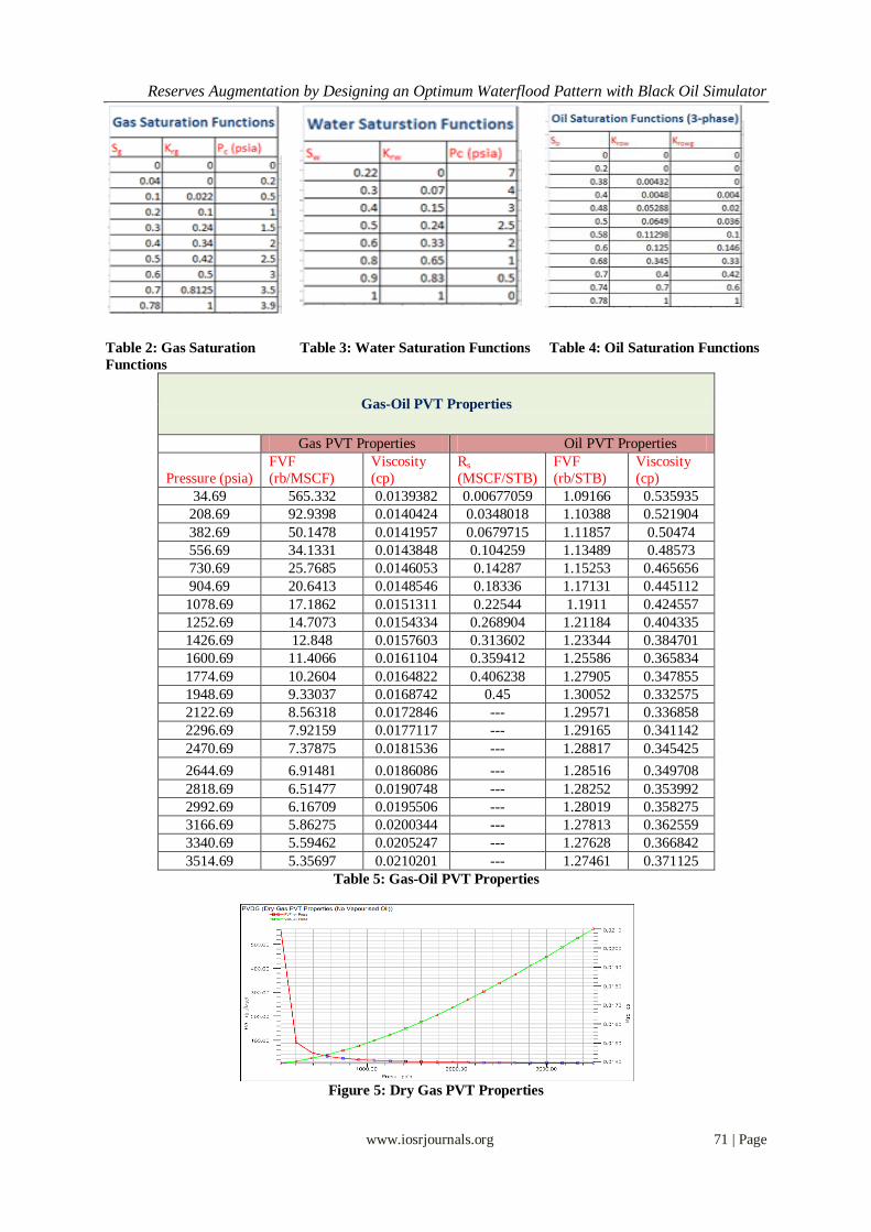
Relative Permeability & Capillary Pressure

Relative permeability verses saturation & capillary pressure data for gas, water and oil (three phase) is

shown in Table 2, 3 & 4.

Fluid Properties The “Reservoir W” will be set to produce by three mechanisms; primary recovery (no injection), five

spot waterflood pattern and nine spot waterflood pattern. The reservoir produces oil of 41 API gravity with no

sulphur, CO2 1% and N2 10% at isothermal conditions of 235F. The connate water has specific gravity of 1, formation volume factor of 1.04569 RB/STB, compressibility of 3.31397E-6 sip and viscosity of 0.291387 cp at

reference pressure of 1948.7 psia. Water salinity is 70,000 and gas gravity is 0.7 (with respect to air). Table 5

gives comprehensive description of the fluid PVT data to be used during this simulation. The graphical

representation of these PVT properties of live oil and dry gas is shown in Figure 5 and 6.

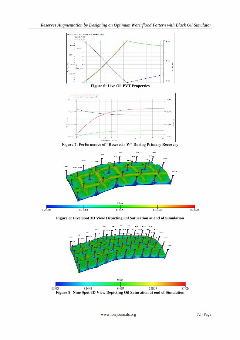
III. Primary Recovery Firstly the “Reservoir W” is set to produce with its primary driving mechanism i.e. solution-gas drive.

When the reservoir pressure is reduced as fluids are withdrawn, gas comes out of the solution and displaces oil

from the reservoir to the producing wells. In “Reservoir W” ten production wells have been landed in to

anticlinal formation and each of it is perforated in all the four layers. Each production well is set to open at a

constant BHP of 1500 psia with maximum flow rate of 4000 STB/D with internal diameter available for fluid

flow is 0.33 ft. Time span for simulation is 30 years.

There are ten production wells naming; “OSAMA”, “P2”, “P3”, “P4”, “P5”, “P6”, “P7”, “P8”, “P9”, “P10”.

Simulation was run for 30 years with strategy described in previous chapter and the results extracted from

Report Generator Module of ECLIPSE E 100 are shown in Table 6.

Table 6: Primary Recovery Results

Average Reservoir Pressure-3139.28 psia

Initial Dissolved Gas-100.57 MMMCF

Average Rs-0.45 MSCF/STB



Average Oil saturation-0.78

Original Oil in Place-223.50 MMSTB

Oil Recovered-50.58 MMSTB

Recovery Factor-22.60 %

Current Reservoir Pressure-1516.7 psia

Current GOR-1.94 MSCF/STB

Current Oil Saturation-0.59445 Current Gas Saturation-0.18428

Current Field Oil in Place-173.301 MMSTB

IV. Problem Statement

The major portion of the “Reservoir W” is not recovered during normal depletion due to decline in

pressure of the reservoir. Out of 223.50 MMSTB OIP (oil in place), 50.58 MMSTB (22.63%) has been

produced after 30 years under solution gas drive reservoir/depletion drive reservoir; which has a weak driving

mechanism and is currently unable to produce oil at economic rate due to decline in its reservoir pressure as

shown in Figure 7. To recover the remaining oil from the reservoir, external energy is required. This required external energy can be given to the reservoir by any secondary recovery method such as waterflooding, during

earlier production stage of “Reservoir W”. After 30 years of production, 173.301 MMSTB remains untapped

within the subject reservoir. Now oil can only be lifted at economic rate from subsurface to the surface, by some

secondary recovery method which sweeps the remaining oil from the reservoir and increases the overall

recovery of the reservoir.

So “Reservoir W” necessarily needs a source of artificial energy or pressure maintenance for

generating handsome revenue for the “Company ABC” and to meet the energy demand of the market. So

regular five spot waterflood pattern and regular nine spot waterflood pattern are developed alternatively to boost

the pressure of the “Reservoir W” and to augment its reserves. Combination of technical and economic analysis

will yield the optimum selection of waterflood pattern for “Reservoir W”.

V. Regular Five Spot Waterflood Pattern Waterflooding is implemented on “Reservoir W” by designing a regular five spot pattern. As the

selection of possible waterflood patterns depends on existing wells that generally must be used because of

economics. Pattern selection is constrained by the location of production wells. “Reservoir W” is developed for

primary production on a uniform well spacing, so five spot pattern will be an intelligent selection.

“Reservoir W” is set to inject water at constant BHP of 2700 psia with 18 injection wells in a 180 acres well

spacing, five spot pattern when pressure of the reservoir falls to bubble point pressure of 1934.07 psia. All the

injection and production wells are perforated in each of the four layers with internal diameter available for flow

is 0.33 ft. Time span for simulation is 30 years. Ten production wells with constraints of constant BHP equal to1500 psia and maximum production

rate of 4000 STB/D started working on 1 Jan 2011 under primary driving mechanism at initial reservoir pressure

of 3514.7 psia. After 1.44 years (527.06 days) of production the reservoir pressure falls to Pb=1934.07 psia. At

this time the 18 injection wells are triggered at above mentioned constraints. This can be done by using

“ACTION” keyword in ECLIPSE E 100 as mentioned in Table 3.1. Until Pb, 11.668 MMSTB (5.22%) of oil has

been recovered. For the next 28.56 years water will be injected. Maximum injection rate during injection span is

44.20 MSTB/D.

Simulation was run for 30 years with strategy described in previous chapter and the results extracted

from Report Generator Module of ECLIPSE E 100 are shown in Table 7.

Table 7: Five Spot Waterflood Result

Average Reservoir Pressure-3139.28 Psia

Initial Dissolved Gas-100.57 MMMCF Average Rs-0.45 MSCF/STB

Average Oil Saturation-0.78

Average Water Saturation-0.22

Average Gas saturation-0




Current Reservoir Pressure-2333.6 Psia

Current Oil Saturation-0.3767

Current water Saturation-0.6297



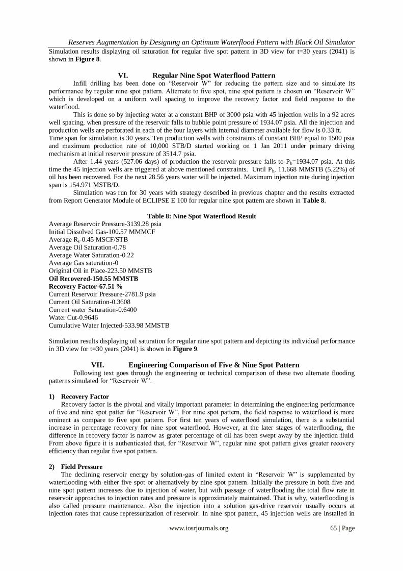
Simulation results displaying oil saturation for regular five spot pattern in 3D view for t=30 years (2041) is

shown in Figure 8.

VI. Regular Nine Spot Waterflood Pattern Infill drilling has been done on “Reservoir W” for reducing the pattern size and to simulate its

performance by regular nine spot pattern. Alternate to five spot, nine spot pattern is chosen on “Reservoir W”

which is developed on a uniform well spacing to improve the recovery factor and field response to the

waterflood.

This is done so by injecting water at a constant BHP of 3000 psia with 45 injection wells in a 92 acres

well spacing, when pressure of the reservoir falls to bubble point pressure of 1934.07 psia. All the injection and

production wells are perforated in each of the four layers with internal diameter available for flow is 0.33 ft.

Time span for simulation is 30 years. Ten production wells with constraints of constant BHP equal to 1500 psia

and maximum production rate of 10,000 STB/D started working on 1 Jan 2011 under primary driving

mechanism at initial reservoir pressure of 3514.7 psia.

After 1.44 years (527.06 days) of production the reservoir pressure falls to Pb=1934.07 psia. At this

time the 45 injection wells are triggered at above mentioned constraints. Until Pb, 11.668 MMSTB (5.22%) of oil has been recovered. For the next 28.56 years water will be injected. Maximum injection rate during injection

span is 154.971 MSTB/D.

Simulation was run for 30 years with strategy described in previous chapter and the results extracted

from Report Generator Module of ECLIPSE E 100 for regular nine spot pattern are shown in Table 8.

Table 8: Nine Spot Waterflood Result

Average Reservoir Pressure-3139.28 psia

Initial Dissolved Gas-100.57 MMMCF

Average Rs-0.45 MSCF/STB

Average Oil Saturation-0.78

Average Water Saturation-0.22 Average Gas saturation-0




Current Reservoir Pressure-2781.9 psia

Current Oil Saturation-0.3608

Current water Saturation-0.6400

Water Cut-0.9646

Cumulative Water Injected-533.98 MMSTB

Simulation results displaying oil saturation for regular nine spot pattern and depicting its individual performance

in 3D view for t=30 years (2041) is shown in Figure 9.

VII. Engineering Comparison of Five & Nine Spot Pattern Following text goes through the engineering or technical comparison of these two alternate flooding

patterns simulated for “Reservoir W”.

1) Recovery Factor

Recovery factor is the pivotal and vitally important parameter in determining the engineering performance

of five and nine spot patter for “Reservoir W”. For nine spot pattern, the field response to waterflood is more

eminent as compare to five spot pattern. For first ten years of waterflood simulation, there is a substantial increase in percentage recovery for nine spot waterflood. However, at the later stages of waterflooding, the

difference in recovery factor is narrow as grater percentage of oil has been swept away by the injection fluid.

From above figure it is authenticated that, for “Reservoir W”, regular nine spot pattern gives greater recovery

efficiency than regular five spot pattern.

2) Field Pressure

The declining reservoir energy by solution-gas of limited extent in “Reservoir W” is supplemented by

waterflooding with either five spot or alternatively by nine spot pattern. Initially the pressure in both five and

nine spot pattern increases due to injection of water, but with passage of waterflooding the total flow rate in

reservoir approaches to injection rates and pressure is approximately maintained. That is why, waterflooding is

also called pressure maintenance. Also the injection into a solution gas-drive reservoir usually occurs at injection rates that cause repressurization of reservoir. In nine spot pattern, 45 injection wells are installed in



“Reservoir W” in contrast with five spot; in which 18 injection wells are used. That’s why pressure is higher in

case of nine spot than in five spot pattern.

3) Cumulative Production

There is greater cumulative production in regular nine spot pattern in comparison with five spot pattern. More

quantity of injection fluid is available and at different location of “Reservoir W” gives greater is to be produced.

The amount of water injected will dictate its percentage of total swept area to total areal coverage of the subject reservoir i.e. areal sweep efficiency is more. So in turn the amount of oil produced at given simulation time is

more in nine spot pattern than in five spot pattern.

4) Oil Production Rate

There are total of 10 production wells with BHP of 1500 psia in each of the five spot and nine spot pattern, but

for five spot pattern each of these production wells are open to flow at surface flow rate of 4000 STB/D and at

10,000 STB/D for nine spot pattern. So initially the oil production rate is much higher in nine spot pattern than

in five spot pattern. However, with passage of time, the oil production rate for nine spot becomes less than of

five spot, as greater quantities of oil has been recovered in earlier life of the project. At the end, the production

rates of both the flooding patterns are nearly equal to one another.

5) Water Injection Rate

Injection rates must exceed reservoir withdrawals if the reservoir pressure is to increase. At higher injection

rates, the oil bank develops more rapidly and reservoir response occurs much sooner. As for “Reservoir W”, the

nine spot pattern has higher ratio of injection to production wells, subsequently it has greater values of injection

rate than that of five spot pattern. At early stage if injection, high injection pressure is needed to produce oil at

respective production rates of five and nine spot, but with injection time the reservoir is repressured so less

injection rate is sufficient to produce oil at assigned production constraints.

6) Cumulative Water Injected

Waterflood performance highly depends upon volume and location of injected water. During first 1.44

simulation years of production, the injection wells are closed. When reservoir pressure drops to bubble point, the

injection wells are triggered. The nine spot pattern requires greater quantities of water to be injected in “Reservoir W” to maintain high production rate than five spot pattern as shown in Figure 10.

7) Water Production Rate

After displacing oil, water injected at a particular rate into reservoir is produced at injection well. When the

production wells are watered-out they are unable to produce oil at desirable rates. The water production rate for

nine spot is very large than that of five spot due to its greater number of wells, high injection pressure and

greater deliverability of production wells.

8) Cumulative Water Produced

The water injected in to reservoir will displace the oil and eventually reaches the production well where it

outcome from the production well. For nine spot pattern very large quantities water is injected. The injected water after sweeping the oil enters the production well. For five spot pattern the increase in production of water

with simulation time is less steep than in case of nine spot pattern as shown in Figure 11.

9) Water Cut

The fractional flow of water is an important parameter in evaluation of recovery performance of five

and nine spot pattern. The fractional flow of water rises abruptly for nine spot pattern as soon as the water

injection is commenced. This might be because of smaller well spacing of water injection and oil production

wells. For five spot pattern as the injection and production wells are far away from each other having greater

well spacing and less number of water injection wells so fractional flow of water increases steadily in

comparison with nine spot pattern. At the later stages waterflooding, much of the oil has been recovered so

percentage of water flowing in the reservoir is much larger than of oil so the Fw rises above 90% for both the flooding patterns

10) WOR

The economic limit of most of the waterflood projects is based usually on water-oil ratio i.e. the

amount of produced water associated with produced oil. It is obvious from the Figure 12 that regular nine spot

pattern has higher values of WOR as compared with regular five spot pattern.



11) Water Saturation

As soon as the waterflooding is initiated on “Reservoir W” after its primary recovery either by five or

nine spot pattern, the saturation of water begins to increase. For nine spot pattern, this increase is more than in

five spot pattern owing to greater water injection wells and their optimum location. After 10 years of

waterflooding, more than 50 % of water saturation has been developed in the pores of “Reservoir W” for both

five and nine spot waterflooding pattern.

12) Oil Saturation

During waterflooding a reservoir its oil saturation is reduced due to withdrawals. Water sweeps a

percentage of oil depending upon the nature of project, but a fraction of oil remains stranded in the porous

media due to different injection schemes for developing reservoir and inherent properties of the reservoir such

as horizontal and vertical heterogeneity, bypassing of injection fluid, low permeability streaks, anisotropy,

wettability and capillary pressure. For five spot pattern the amount of unswept oil is more than that for nine spot

pattern.

Engineering Comparison of Five & Nine Spot Pattern: Results The complete engineering analysis and performance evaluation of “Reservoir W” using regular nine spot

waterflood pattern and of regular five spot waterflood pattern with the help of Black Oil Simulator explicitly shows that the regular nine spot pattern gives greater recovery efficiency [Figure 13 & 14] and is advisable to

plan a nine spot waterflood injection scheme for this reservoir. However, as nine spot waterflood pattern has

more injection wells comparable with five spot pattern which obviously requires high capital investment, so

economic analysis will be the conclusive and decisive factor in ultimate selection of waterflooding pattern on

“Reservoir W”.

VIII. Financial / Economic Comparison of Five & Nine Spot Pattern In today’s world, economics control the decision making process for future projection. For the last two

decades, energy supply has suffered from a series of oil crises e.g. BP oil spill in Gulf of Mexico (2010). This forces reservoir and production engineers to direct their attention to study the economic performance of oil and

gas fields. The study utilizes the data generated by the Black Oil Simulator primary recovery, regular five spot

and regular nine spot pattern for economic evaluation of the production projections and assessment of these

investment opportunities to select the economically optimum case for profit generation.

The tasks included are:

Developing an economic model based on net cash flow concepts to study the different alternatives for field

development.

Calculating Before & After-Tax Net Cash Flow for the economic model

Studying the effect of time value of money by introduction of an arbitrary discount rate

Economic Comparison of all the investment opportunities

Case A: Economic Analysis of Base Case (Primary Recovery)

The Parameters shown in the Table 9 are assumed for oil production under primary recovery for 30

years in the economic model. The operating cost of the base case is assumed in accordance with current

operating conditions provided by “Company ABC”. The initial investment for primary recovery is 210 million

dollars. The economic calculations of the base case are summarized in the Table 10 & 11.

Table 9: Primary Recovery Economic Parameters & Worth

Parameter-Worth

Oil Price [Brent crude oil]-90 ($/bbl)

Royalty-20% State Taxes [Severance/Ad valorem]-12%

Operating Cost-10 ($/bbl)

Over head % of Operating Cost-30%

Capital Investment-200 (MM$)

Bonus &Leasehold Cost-10 (MM$)

Income Tax Rate-30%

Discount Rate-10%



Case B: Economic Analysis of Augmented Case

(Five Spot Waterflood Pattern)

The Parameters shown in the Table 9 are assumed for oil production and water injection methods in the

economic model.

Table 9: Five Spot Waterflood

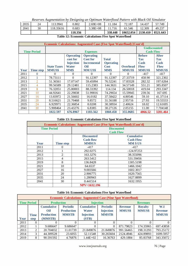
The operating cost for augmented case is assumed same as the current operating cost to reflect the fact

that the incremental production will enjoy the existence of surface facilities capable of treating the additional

production with virtually no operating cost. The initial investment for regular five spot pattern is 417 million dollars. The economic calculations of the five spot waterflood are summarized in the Table 12, 13 & 14.

Case C: Economic Analysis of Augmented Case

(Nine Spot Waterflood Pattern)

The Parameters shown in the Table 15 are assumed for oil production and water injection methods in the

economic model.

The initial investment for regular five spot pattern is 713 million dollars. The economic calculations of the

augmented case are summarized in the Table 16, 17 & 18.

Economic Comparison of Five & Nine Spot Pattern: Results

The calculations show the economic analysis and productivity of three different investment proposals.

The best measure of the economic worth of the investment proposals is their ability to generate profit. The net present value for Case A (base case) is 875.757 million dollars as shown by the discounted

cash flow calculations at the discount rate of 10% if “Reservoir W” is produced under its primary driving

mechanism for 30 years with capital investment of 210 MM US $. However, if Case B (five spot waterflooding)

is practically implemented on “Reservoir W”, then the net present worth of this investment opportunity will

augment from 875.757 MM US$ to 1632.196 MM US$. Although the initial investment required for this is 261

MM US$ more than that required for base case, the profit generated is phenomenal i.e.756.439 MM US$ more

than primary recovery.

The Case C (nine spot waterflood) does not show fruitful results as compared with five spot pattern.

The net present value decreases from 1632.196 MM US$ to 1561.026 MM US$. The initial investment required

is very large i.e. 7.13 billion US dollars. Also the cash flow for last three years is negative; the operating

expenses exceed the revenue generated. Figure 15 & 16 shows the comparison of NPV and capital investment for all the cases.



Table 15: Nine Spot Waterflood

IX. Conclusion The engineering and economic study depicts that the “Reservoir W” necessarily needs implementation of

waterflooding The economic model developed for primary recovery, regular five spot waterflood and regular nine spot waterflood shows that the economical investment opportunity will be five spot waterflood, as it

generates handsome revenue and profit for “Company ABC”. Although the recovery efficiency of nine spot

waterflood is large, but its high capital investment and low profitability makes it an unfavorable option for

subject reservoir. But the crux is that the oil and gas exploration and production are inherently probabilistic. By

their very nature they include large element of risks and uncertainties. That is why petroleum exploitation is

always an exciting and challenging game----a game of chance but also of change.

X. Recommendations

On the basis of this study, I recommend the following:

Reducing the pattern size of either five or nine spot pattern to 40 acres and investigating its impact on

recovery.

Selective plugging of either layer(s) can reduce the early breakthrough at production wells

Delve the effect of salinity on waterflooding for improving recovery efficiency.

Investigate the technical and economic impact of installing sucker rod pumps on each of the production

wells.

Adopt a monitoring plan for monitoring of production or pressure data e.g. installing SCADA on the

production facility.

Streamline simulation can be helpful in better field management and pattern balancing.

XI. Acknowledgement I am grateful to operating company OGDCL for providing technical data, Schlumberger for offering

license of ECLIPSE 2008.1 & tribute to all the scientists and researchers who have a capability of “seeing

underground” and have made significant contribution in understanding of petroleum reservoirs which are one of

the nature’s ubiquitous and diverse materials. As;

“There are worlds to see in the grain of sand”.

An expression of gratitude to Dr. Obed-ur-Rehman Paracha & Dr. Saeed Khan Jadoon for their

guidance and to my senior Mr. Bilal Amjad for his valuable suggestions and assistance.

Bibliography

1. ECLIPSE 2008.1, “Technical Description”. (2008)

2. ECLIPSE 2008.1, “Reference Manual”. (2008)



Figure 1: “Reservoir W” TOPS of First Layer

Figure 2: “Reservoir W” Porosity of First Layer

Figure 3: “Reservoir W” Permeability of First Layer:

Figure 4: Porosity & PermX Variation of Individual Layers of “Reservoir W”



Table 2: Gas Saturation Table 3: Water Saturation Functions Table 4: Oil Saturation Functions

Functions

Gas-Oil PVT Properties

Gas PVT Properties Oil PVT Properties

Pressure (psia)

FVF

(rb/MSCF)

Viscosity

(cp)

Rs

(MSCF/STB)

FVF

(rb/STB)

Viscosity

(cp)

34.69 565.332 0.0139382 0.00677059 1.09166 0.535935

208.69 92.9398 0.0140424 0.0348018 1.10388 0.521904

382.69 50.1478 0.0141957 0.0679715 1.11857 0.50474

556.69 34.1331 0.0143848 0.104259 1.13489 0.48573

730.69 25.7685 0.0146053 0.14287 1.15253 0.465656

904.69 20.6413 0.0148546 0.18336 1.17131 0.445112

1078.69 17.1862 0.0151311 0.22544 1.1911 0.424557

1252.69 14.7073 0.0154334 0.268904 1.21184 0.404335

1426.69 12.848 0.0157603 0.313602 1.23344 0.384701

1600.69 11.4066 0.0161104 0.359412 1.25586 0.365834

1774.69 10.2604 0.0164822 0.406238 1.27905 0.347855

1948.69 9.33037 0.0168742 0.45 1.30052 0.332575

2122.69 8.56318 0.0172846 --- 1.29571 0.336858

2296.69 7.92159 0.0177117 --- 1.29165 0.341142

2470.69 7.37875 0.0181536 --- 1.28817 0.345425

2644.69 6.91481 0.0186086 --- 1.28516 0.349708

2818.69 6.51477 0.0190748 --- 1.28252 0.353992

2992.69 6.16709 0.0195506 --- 1.28019 0.358275

3166.69 5.86275 0.0200344 --- 1.27813 0.362559

3340.69 5.59462 0.0205247 --- 1.27628 0.366842

3514.69 5.35697 0.0210201 --- 1.27461 0.371125

Table 5: Gas-Oil PVT Properties

Figure 5: Dry Gas PVT Properties



Figure 6: Live Oil PVT Properties

Figure 7: Performance of “Reservoir W” During Primary Recovery

Figure 8: Five Spot 3D View Depicting Oil Saturation at end of Simulation

Figure 9: Nine Spot 3D View Depicting Oil Saturation at end of Simulation



Figure 10: Five & Nine Spot Cumulative Water Injected

Figure 11: Five & Nine Spot Cumulative Water Produced

Figure 12: Five & Nine Spot WOR



Figure 15: Net Present Value of Investment Opportunities

Figure 16: Capital Investment for Investment Opportunities

Economic Calculations: Base Case (Primary Recovery)

Time Period Production Revenues Expenses

Year

Tim

e

step

Cumulativ

e

Productio

n

(MMSTB)

Periodic

Productio

n

(MMSTB)

Revenu

e MM

(US$)

Royalt

y MM

(US$)

W.I

Revenu

e MM

(US$)

State

Taxes

(MM)

(US$)

Operatin

g

Cost[MM

US$]

Overhea

d MM

US $

201

1 0 0 --- 0 0 0 0 0 0

201

2 1 9.112397 9.112397 820.11 164.02 656.09 78.73 91.12397

27.33719

1

201

3 2 14.71215 5.599751 503.97 100.79 403.18 48.38 55.99751

16.79925

3

201

5 4 24.10456 4.437654 399.38 79.87 319.51 38.34 44.37654

13.31296

2

201

7 6 31.50287 3.478742 313.08 62.61 250.46 30.05 34.78742

10.43622

6

201

9 8 37.15996 2.62164 235.94 47.18 188.75 22.65 26.2164 7.86492

202

1 10 41.33776 1.919564 172.76 34.55 138.20 16.58 19.19564 5.758692



202

3 12 44.28119 1.334356 120.09 24.01 96.07 11.52 13.34356 4.003068

202

5 14 46.28373 0.903284 81.29 16.25 65.03 7.80 9.03284 2.709852

202

7 16 47.63676 0.610688 54.96 10.99 43.96 5.27 6.10688 1.832064

203

1 20 49.19995 0.29066 26.15 5.23 20.92 2.51 2.9066 0.87198

203

5 24 49.95673 0.141568 12.74 2.54 10.19 1.22 1.41568 0.424704

2039 28 50.3217 0.06718 6.04 1.20 4.83 0.58 0.6718 0.20154

204

1 30 50.42097 0.044364 3.99 0.79 3.19 0.38 0.44364 0.133092

50.42 4537.88 907.57 3630.30

435.6

3 504.20 151.26

Table 10: Economic Calculations Primary Recovery

Economic Calculations: Base Case (Primary Recovery) [Cont'd]

Time Period Cash Flow

Year

Time

step

Before Tax

Net Cash

Flow

(MM US $)

After Tax

Net Cash

Flow

(MM US $)

Discounted

Cash flow

(MM $ US)

Cumulative

Cash Flow

(MM $ US)

2011 0 -210 -210 -210 -210

2012 1 458.9003129 321.230219 292.0274719 82.02747186

2013 2 282.0034604 197.4024223 163.1424977 245.1699696

2015 4 223.4802554 156.4361788 106.848015 483.2465872

2017 6 175.1894471 122.632613 69.222913 638.2637332

2019 8 132.0257904 92.41805328 43.11370392 736.2882722

2021 10 96.66924304 67.66847013 26.08912456 796.1386184

2023 12 67.19816816 47.03871771 14.98798509 831.0077699

2025 14 45.48938224 31.84256757 8.385143258 850.6176896

2027 16 30.75424768 21.52797338 4.685114241 861.5674471

2031 20 14.6376376 10.24634632 1.523054091 871.2781328

2035 24 7.12936448 4.990555136 0.506669095 874.4874088

2039 28 3.3831848 2.36822936 0.164220956 875.5454566

2041 30 2.23417104 1.563919728 0.089625977 875.7570938

2329.200 1567.440 NPV= 875.757

Table 11: Economic Calculations Primary Recovery

Economic Calculations: Augmented Case (Five Spot Waterflood)

Time Period Production Injection Revenues

Year Time step

Cumulative Periodic Cumulative Periodic Revenue Royalty W.I

Oil Production Water Injection MMUS$ MMUS$ Revenue

Production MMSTB Injection MMSTB

MMUS$

(MMSTB)

(STB)

2011 0 0 0 0 0 0 0 0

2012 1 9.112397 9.112 0 0 820.115 164.023 656.092

2013 2 15.057491 5.945 8535735 8.535 535.058 107.011 428.046

2015 4 35.867292 11.523 38541484 14.562 1037.147 207.428 829.715

2019 8 78.193864 8.833 94293720 12.9 795.005 159.001 636.004

2021 10 90.285328 5.199 1.17E+08 11.149 467.983 93.596 374.386

2027 16 105.855 1.601 1.82E+08 10.783 144.163 28.832 115.331

2031 20 110.54658 0.985 2.25E+08 10.852 88.714 17.742 70.971



2035 24 113.9941 0.802 2.69E+08 11.184 72.187 14.437 57.749

2041 30 118.35616 0.683 3.38E+08 11.716 61.546 12.309 49.237

118.356

338.448 10652.054 2130.410 8521.643

Table 12: Economic Calculations Five Spot Waterflood

Economic Calculations: Augmented Case (Five Spot Waterflood) [Cont'd]

Time Period Expenses

Undiscounted

Cash Flow

Year Time step

State Taxes

MMUS$

Operating

cost for

Injection

Water

MM$

Operating

Cost for

Incremental

Oil

MM US$

Total

Operating

Cost

MM$

Overhead

MMUS$

Before

Tax

Cash

Flow

MMUS$

After

Tax

Cash

Flow

MMUS$

2011 0 0 0 0 0 0 -417 -417

2012 1 78.73111 0 91.12397 91.12397 27.33719 458.90 321.2302

2013 2 51.36561 17.07147 59.45094 76.52241 17.83528 282.32 197.6264

2015 4 99.56589 29.12481 115.2383 144.3631 34.57149 551.21 385.8507

2019 8 76.32051 25.80003 88.33392 114.134 26.50018 419.04 293.3347

2021 10 44.92641 22.29838 51.99816 74.29654 15.59945 239.56 167.695

2027 16 13.83972 21.56602 16.0182 37.58422 4.80546 59.10 41.37114

2031 20 8.516621 21.70468 9.8572 31.56188 2.95716 27.93 19.55533

2035 24 6.929971 22.36854 8.0208 30.38934 2.40624 18.02 12.61695

2041 30 5.908464 23.43276 6.8385 30.27126 2.05155 11.00 7.704148

1022.597 676.8967 1183.562 1860.458 355.0685 4866.52 3281.464


Economic Calculations: Augmented Case (Five Spot Waterflood) [Cont'd]

Time Period

Discounted

Cash Flow

Year Time step

Discounted

Cash flow

MM$US

Cumulative

Cash Flow

MM $ US

2011 0 -417 -417

2012 1 292.0275 -124.97253

2013 2 163.3276 38.355096

2015 4 263.5412 531.59456

2019 8 136.8428 1305.5198

2021 10 64.6537 1466.1042

2027 16 9.003566 1602.3017

2031 20 2.906775 1620.7565

2035 24 1.280943 1627.8899

2041 30 0.441514 1632.1955

NPV=1632.196


Economic Calculations: Augmented Case (Nine Spot Waterflood)

Time Period Production Injection Revenues

Year

Time

step

Cumulative Periodic Cumulative Periodic Revenue Royalty W.I

Oil Production Water Injection MMUS$ MMUS$ Revenue

Production MMSTB Injection MMSTB

MMUS$

(MMSTB)

(STB)

2011 0 0 0 0 0 0 0 0

2012 1 9.686647 9.686647 0 0 871.79823 174.35965 697.43858

2013 2 20.704032 11.01739 21.849876 21.849876 991.56465 198.31293 793.25172

2014 3 44.309528 23.6055 52.11548 30.265604 2124.4946 424.89893 1699.5957

2019 8 90.591592 4.76876 1.44E+02 16.36763 429.1884 85.83768 343.35072



2021 10 97.797408 3.199112 1.77E+02 16.4766 287.92008 57.584016 230.33606

2027 16 108.26086 1.21308 2.77E+02 16.80898 109.1772 21.83544 87.34176

2031 20 112.43228 0.9625 3.46E+02 17.60519 86.625 17.325 69.3

2035 24 115.9649 0.84124 4.18E+02 18.31398 75.7116 15.14232 60.56928

2039 28 119.0932 0.74886 4.93E+02 18.9473 67.3974 13.47948 53.91792

2041 30 120.53038 0.7088 5.31E+02 19.24221 63.792 12.7584 51.0336

120.5304 530.93235 10847.734 2169.5468 8678.1874

Table 16: Economic Calculations Nine Spot Waterflood

Economic Calculations: Augmented Case (Nine Spot Waterflood) [Cont'd]

Time Period Expenses

Undiscounted

Cash Flow

Year

Time

step

State

Taxes

MMUS$

Operating

cost for

Injection

Water

MM$

Operating

Cost for

Incremental

Oil

MM US$

Total

Operating

Cost

MM$

Overhead

MMUS$

Before

Tax

Cash

Flow

MMUS$

After

Tax

Cash

Flow

MMUS$

2011 0 0 0 0 0 0 -713 -713

2012 1 83.69263 0 96.86647 96.86647 29.05994 487.8195 341.4737

2013 2 95.19021 43.69975 110.1739 153.8736 33.05216 511.1358 357.795

2014 3 203.9515 60.53121 236.055 296.5862 70.81649 1128.242 789.7691

2019 8 41.20209 32.73526 47.6876 80.42286 14.30628 207.4195 145.1936

2021 10 27.64033 32.9532 31.99112 64.94432 9.597336 128.1541 89.70786

2027 16 10.48101 33.61796 12.1308 45.74876 3.63924 27.47275 19.23092

2031 20 8.316 35.21038 9.625 44.83538 2.8875 13.26112 9.282784

2035 24 7.268314 36.62796 8.4124 45.04036 2.52372 5.736886 4.01582

2039 28 6.47015 37.8946 7.4886 45.3832 2.24658 -0.18201 -0.12741

2041 30 6.124032 38.48442 7.088 45.57242 2.1264 -2.78925 -1.95248

1041.382 1061.865 1205.304 2267.169 361.5911 4295.045 2792.632


Economic Calculations: Augmented Case (Nine Spot Waterflood) [Cont'd]

Time Period

Discounted

Cash Flow

Year Time step

Discounted

Cash flow

MM$US

Cumulative

Cash Flow

MM $ US

2011 0 -713 -713

2012 1 310.4306 -402.569

2013 2 295.6984 -106.871

2014 3 593.3652 486.4942

2019 8 67.73391 1395.684

2021 10 34.58626 1480.413

2027 16 4.185209 1549.019

2031 20 1.379827 1557.896

2035 24 0.407709 1560.725

2039 28 -0.00883 1561.205

2041 30 -0.11189 1561.026

NPV=1561.026


Documents

Reserves Augmentation by Designing an Optimum Waterflood Pattern with Black Oil Simulator