Embed Size (px)
Citation preview

www.csgb.dk
RESEARCH REPORT 2015
CENTRE FOR STOCHASTIC GEOMETRYAND ADVANCED BIOIMAGING
Abdollah Jalilian, Yongtao Guan, Jorge Mateu and Rasmus Waagepetersen
Multivariate Product-Shot-noise Cox Point Process Models
No. 05, April 2015

Multivariate Product-Shot-noise Cox Point Process Models
Abdollah Jalilian1, Yongtao Guan2, Jorge Mateu3 and Rasmus Waagepetersen4∗
April 10, 2015
Abstract
We introduce a new multivariate product-shot-noise Cox process which is useful for model-ing multi-species spatial point patterns with clustering intra-specific interactions and neutral,negative or positive inter-specific interactions. The auto and cross pair correlation functionsof the process can be obtained in closed analytical forms and approximate simulation of theprocess is straightforward. We use the proposed process to model interactions within andamong five tree species in the Barro Colorado Island plot.
Keywords: Cox process; Cross pair correlation function; Inter-specific interactions; Multivariatepoint process; Product fields.
1 Introduction
In forestry and plant ecology, there are many factors affecting the spatial patterns of species lo-cations. Habitat preferences and variations in environmental conditions cause inhomogeneity at alarge scale (Law et al., 2009). The effects of factors such as dispersal strategies, pathogen transmis-sion, resource competition, allelopathy, predation and facilitation moreover create interactions at alocal scale between neighbouring trees (Wootton and Emmerson, 2005; Illian and Burslem, 2007).The interactions are either intra-specific (between individuals of the same species) or inter-specific(between trees of different species) (Wiegand et al., 2007).
Spatial point process models and their summary statistics are widely used to analyze fullymapped species locations (see e.g. Stoyan and Penttinen, 2000; Comas and Mateu, 2007; Illianand Burslem, 2007) and can provide insight regarding the underlying community dynamics andcoexistence mechanisms (Wiegand et al., 2007; Luo et al., 2012). For a single species, the intra-specific interaction may be positive (clustered), negative (repulsive) or neutral. Second-ordercharacteristics such as Ripley’s K-function and the pair correlation function are useful for detect-ing these types of interactions (Stoyan and Penttinen, 2000; Comas and Mateu, 2007). Most oftenthe intra-specific interactions are either clustered or random (Picard et al., 2009b). UnivariateCox processes are therefore useful for modeling such interactions as well as spatial inhomogene-ity (Waagepetersen, 2007; Waagepetersen and Guan, 2009).
For multiple species, the inter-specific interactions can be far more complex. One species mayhave positive (+), negative (−) or neutral (0) effect on the other species. Thus for any pair ofspecies, the inter-specific interaction can be one of six possible types, namely, neutralism (0, 0),competition (−,−), mutualism (+,+), amensalism (−, 0)/(0,−), commensalism (+, 0)/(0,+) andpredation (+,−)/(−,+) (Nathaniel Holland and DeAngelis, 2009). To detect these interactions,second-order characteristics designed for multivariate point processes, such as the cross K- andcross pair correlation functions, can be used for both stationary and nonstationary processes (Co-mas and Mateu, 2007; Baddeley et al., 2000). Lieshout and Baddeley (1999) introduced further
∗1Department of Statistics, Razi University, Bagh-e-Abrisham, Kermanshah 67149-67346, Iran,[email protected]. 2Department of Management Science, University of Miami, Coral Gables, Florida33124-6544, U.S.A, [email protected]. 3Department of Mathematics, Universitat Jaume I, Castellon E-12071,Spain, [email protected]. 4Department of Mathematical Sciences, Aalborg University, Fredrik Bajersvej 7G,DK-9220 Aalborg, Denmark, [email protected]
1

summary statistics which, unlike the cross K- and cross pair correlation functions, consider asym-metry in the effects of two species on each other. However, these summary statistics are restrictedto the stationary case.
The literature on modeling multivariate spatial point patterns is mainly restricted to the bivari-ate case. Harkness and Isham (1983), Grabarnik and Sarkka (2009) and Picard et al. (2009a) forexample introduced various parametric stationary multivariate Gibbs models for the coexistencemechanisms in homogeneous animal or plant communities. However, Gibbs point processes oftenare not appropriate for modeling clustering intra-specific interactions. Cox processes, on the otherhand, are more flexible. As an early attempt to develop multivariate Cox processes, Diggle andMilne (1983) considered bivariate Cox processes driven by proportional random intensities (linkedCox processes) and random intensities with a constant sum (balanced Cox processes). A linkedCox process can be thought of as an extreme case of inter-specific interaction of type mutualismwhile a balanced Cox process is appropriate for the cases where the two species compete for aconstant amount of resources. These bivariate Cox models are restrictive since there is a very rigidrelation between the random intensity functions. Møller et al. (1998), Brix and Møller (2001) andLiang et al. (2009) developed more flexible multivariate log-Gaussian Cox process models. How-ever, certain types of clustering due to for example seed dispersal are not naturally covered bylog-Gaussian Cox process models.
In the present paper we introduce a new parametric class of multivariate product-shot-noiseCox point process models. Our proposed model incorporates both spatial inhomogeneity and allthe six types of inter-specific interactions described earlier. We obtain closed form expressions forboth the auto (i.e., univariate) and cross pair correlation functions. The model is applied to adata example of tree locations which contains five species. This example is challenging comparedwith the bivariate examples that are most often considered when parametric models are usedfor multivariate point patterns. Apart from ecology, the new models could also be applied inepidemiology where it could be of interest to study simultaneously the spatial patterns of cases ofseveral types of diseases.
2 Point process background
Let X1, . . . , Xm be the underlying point processes that govern the spatial distributions of mspecies in a given geographical region W ⊂ R2. For i 6= j = 1, . . . ,m, let ρi : W → [0,∞) andgii : W ×W → [0,∞) respectively be the intensity and (auto) pair correlation function of Xi, andlet gij : W ×W → [0,∞) be the cross pair correlation function of Xi and Xj . Then the intensityand the pair correlation function of the multivariate point process X = (X1, . . . , Xm) are given byρ(u) =
(ρ1(u), . . . , ρm(u)
)and g(u, v) = [gij(u, v)]ij (Møller and Waagepetersen, 2004).
The intensity function ρ controls spatial inhomogeneity of all species over W . Spatial inhomo-geneity is often related to spatially varying environmental variables z1(u), . . . , zp(u) such as soilconditions and topographical variables. It is common to use a log-linear model
ρi(u;βi) = exp
{βi0 +
p∑
l=1
βilzl(u)
}, i = 1, . . . ,m, (1)
for this relation where βi = (βi0, βi1, . . . , βip) ∈ Rp+1 is a vector of regression parameters for theith species (Waagepetersen, 2007; Waagepetersen and Guan, 2009; Renner and Warton, 2013).
The pair correlation function g quantifies the within- and between-species correlation of X.In the sequel we say that the correlation is positive if gij > 1 and negative if gij < 1. As wedescribed in Section 1, there are six different types of interactions. Some of these interactionsresult in qualitatively similar cross pair correlation functions. For example, (+,+), (0,+) and(+, 0) all yield positive correlations, i.e. gij > 1 and gji > 1.
If the components of X, X1, . . . , Xm, are Cox processes driven by random intensity functions
2

Table 1: Possible parametric choices for kernel function k with corresponding kernel convolutioncovariance function R.
k(u) R(u)
Gaussian 12πω2 exp
(− ‖u‖2
2ω2
)1
4πω2κexp
(− ‖u‖2
4ω2
)
Variance gamma (‖u‖/ω)νKν(‖u‖/ω)
πω22ν+1Γ(ν+1)1
πω222ν+2Γ(2ν+2)κ
(‖u‖ω
)2ν+1
K2ν+1
(‖u‖ω
)
Cauchy 12πω2
(1 + ‖u‖2
ω2
)−1.51
8πω2κ
(1 + ‖u‖2
4ω2
)−1.5
Λ1(u), . . . ,Λm(u), respectively, then ρi(u) = EΛi(u), i = 1, . . . ,m, and
gij(u, v) =EΛi(u)Λj(v)
EΛi(u)EΛj(v)= 1 +
Cov(Λi(u),Λj(v))
ρi(u)ρj(v), i, j = 1, . . . ,m, (2)
see Møller and Waagepetersen (2004), Section 5.8. Thus for a multivariate Cox process, there is aclose connection between the pair correlation function of X and the covariance function of the latentprocess Λ(u) =
(Λ1(u), . . . ,Λm(u)
). More specifically, correlations between and within random
fields Λi’s create correlations between and within species Xi’s. In order to construct multivariateCox processes with desired types of interactions, appropriate nonnegative multivariate randomfields are needed. In the case of multivariate log-Gaussian Cox process (Møller et al., 1998),Λ(u) = exp
(Ψ(u)
)where Ψ is a multivariate Gaussian random field. In this paper we develop a
different multivariate random field that has more explicit biological interpretations.
3 A multivariate Product-shot-noise Cox process
3.1 Shot-noise fields
For i = 1, . . . ,m, let
Si(u) =1
κi
∑
v∈Φi
ki(u− v) (3)
be a shot-noise field generated by a stationary Poisson process Φi on R2 with intensity κi > 0and a bivariate probability density function ki. Thus, Si(u) is formed by superposition of randomimpulses ki(u − v) for the points v ∈ Φi (Illian et al., 2008, p. 45). A Cox process Xi driven bya random intensity function proportional to Si(u) is called a shot-noise Cox process with parentprocess Φi and dispersal kernel ki (Møller, 2003). Since ESi(u) = 1, the pair correlation functionof Xi is given by
gSi (u, v) = ESi(u)Si(v) = 1 +Ri(u− v),
where
Ri(h) =1
κi
∫
R2
ki(h+ v)ki(v)dv (4)
is a kernel convolution covariance function (Matern, 1986; Jalilian et al., 2013). Three possiblechoices for the dispersal kernel ki are given in Table 1.
It follows from gSi (u, v) ≥ 1 that Xi is a clustered point process. To obtain inter-specific in-teractions, one may consider dependent parent processes Φ1, . . . ,Φm (Møller and Waagepetersen,2004, Section 3.3.2 and Section 5.8.3). However, with this approach it is difficult to derive flexiblemodels with tractable cross pair correlation functions. Instead, we assume that Φi’s are indepen-dent and model the dependence between Xi’s by using additional so-called product fields.
3

3.2 Product fields
As an alternative to the additive superposition in (3), we consider multiplicative superposition ofimpulses from the parent process Φi and define the product fields
Eli(u) = exp{− κlξli/kl(0)
} ∏
w∈Φl
{1 + ξlikl(u− w)
}, l 6= i = 1, . . .m, (5)
where ξli ∈ (−1,∞) and kl(u) = kl(u)/kl(0) is a scaled version of kl. Here, the contribution of
w ∈ Φl to Eli(u) is 1 + ξlikl(u−w), which may increase (ξli > 0), decrease (−1 < ξli < 0) or doesnot change (ξli = 0) the overall value of Eli(u). More specifically, ξli > 0 implies that Eli(u) takeslarger values around points of Φl while −1 < ξli < 0 implies the opposite. Thus, the sign of ξlidetermines the nature of impact of Φl (and hence Xl) on Xi. The shape, range and strength of thisimpact is controled by the shape and tail behavior of the kernel function kl and the magnitude of
ξli. The product fields (5) can be rewritten as exp[−κlξli/kl(0) +
∑w∈Φl
log{
1 + ξlikl(u− w)}],
which is similar to the log shot-noise field used for univariate modeling in Hellmund et al. (2008),
except that log[1 + ξlikl(u− w)
]is not a kernel function.
Based on the product fields (5), we define a set of compound fields
Fi(u) =∏
l 6=iEli(u) = exp
∑
l 6=i
κlξlikl(0)
∏
l 6=i
∏
w∈Φl
{1 + ξlikl(u− w)
}, i = 1, . . . ,m.
Thus, Fi is the overall impact of all other species on the ith species. Each Fi is stationary withmean EFi(u) = 1. Let
cl(h) =κl
kl(0)2Rl(h) =
1
kl(0)2
∫
R2
kl(h+ v)kl(v)dv,
It can be shown (see Appendix) that a multivariate Cox process driven by F(u) =(F1(u), . . . , Fm(u)
)
has auto pair correlation functions
gFii (h) = exp
∑
l 6=iκlξ
2licl(h)
≥ 1. (6)
Thus, the random field F produces clustering intra-specific interactions. If ξli is positive, thenpoints of Xi cluster around points of Φl. If ξli is negative, then points of Xi are repelled by pointsof Φl which again introduces positive correlations in Xi. Moreover, the cross pair correlations are
gFij(u− v) = EFi(u)Fj(v) = exp
∑
l 6=i,jκlξliξljcl(u− v)
, i 6= j = 1, . . . ,m. (7)
Depending on ξliξlj , l 6= i, j, the terms κlξliξljcl(u− v) in (7) can be negative or positive, leadingto negative or positive inter-specific correlations, respectively. For example, if ξli and ξlj are ofopposite signs, repulsion between Xi and Xj is introduced since the points of Xi and Xj arerespectively attracted and repelled by points of Φl. Note that the signs of ξli and ξlj can beinterchanged without changing gFij .
3.3 The new multivariate Cox process model
We now combine the shot-noise and product fields described in the previous sections to obtain ournew multivariate product-shot-noise Cox process model. Let X1, . . . , Xm be Cox point processeswith random intensity functions
Λi(u) = ρi(u)Si(u)Fi(u), i = 1, . . . ,m. (8)
4

The term ρi(u) = EΛi(u) is the intensity function of Xi and represents spatial inhomogeneityof the ith species. We assume that the ρi’s are either constant for homogeneous species or inthe log-linear form (1) for inhomogeneous species. The shot-noise term Si accounts for clusteringin the ith species due to regeneration mechanisms such as seed dispersal and root propagation.The ith compound field Fi in (8) represents the effect of the other species on the ith speciesand excluding it from the model, or equivalently letting the ξij = 0, implies that X1, . . . , Xm
are independent shot-noise Cox processes. Referring to the six types of inter-specific interactionsdescribed in Section 1, ξij and ξji being both negative would correspond to competition (−,−)between Xi and Xj , ξij and ξji being both positive would correspond to mutualism (+,+) etc.
According to (8), X = (X1, . . . , Xm) is a multivariate Cox process. Assuming that the kernelski are bounded, the intensity function is ρ(u) =
(ρ1(u), . . . , ρm(u)
)and the auto pair correlation
functions (see the Appendix for derivations) are
gii(h) = gSi (h)gFii (h) =
{1 +
ki(0)2
κici(h)
}exp
∑
l 6=iκlξ
2licl(h)
, i = 1, . . . ,m. (9)
Thus, the pair correlation function gii is a product of the shot-noise pair correlation function gSiand the pair correlation function gFii (h). Note that gii(h) > gSi (h) and gii(h) > gFii (h), whichmeans that realizations of a Cox process driven by (8) are more clustered than realizations ofa Cox process driven by either the shot-noise field Si or the compound field Fi. The cross paircorrelation functions are further given by (see Appendix)
gij(h) ={
1 +κiξijki(0)
Ri(h)}{
1 +κjξjikj(0)
Rj(h)}gFij(h)
={
1 + ξijki(0)ci(h)}{
1 + ξjikj(0)cj(h)}
exp
∑
l 6=i,jκlξliξljcl(h)
. (10)
The first and second factor in the cross pair correlation function gij(h) represent correlation due tothe direct effect of species i on j and vice versa, while the term gFij(h) accounts for the correlation
induced by the effects of all other species on species i and j. In fact, gij(h)/gFij(h) is closely relatedto a type of partial correlation between species i and species j controling for the effect of all otherspecies. More precisely, up to a multiplicative constant, gij(h)/gFij(h) − 1 is the lag h partialcorrelation Corr{Λi(u),Λj(u+ h)|Φk, k 6= i, j} between the latent fields Λi and Λj conditional onthe latent processes Φk, k 6= i, j. Thus ξij = ξji = 0 implies that the partial correlation is zero andcorrelation between species i and j is then solely due to influence of the Φk processes for the otherspecies k 6= i, j. The cross pair correlation functions (10) are translation invariant and symmetricin the sense that gij(u − v) = gji(u − v) and gij(u − v) = gij(v − u). For the choices of kernelfunctions in Table 1 we also have isotropy so that gij(h) only depends on ‖h‖.
3.4 A numerical example
Figure 1 shows gij ’s for m = 3 species, κ = (20, 35, 30), Gaussian kernels with bandwidthsω = (0.035, 0.03, 0.02) and interaction parameters
ξ =
0 0.3 −0.60.8 0 0.9−0.9 −0.9 0
.
5

Here
g12(h) =
{1 +
ξ12
2exp
(−‖h‖
2
4ω21
)}{1 +
ξ21
2exp
(−‖h‖
2
4ω22
)}exp
{κ3ξ31ξ32c3(h)
},
g13(h) =
{1 +
ξ13
2exp
(−‖h‖
2
4ω21
)}{1 +
ξ31
2exp
(−‖h‖
2
4ω23
)}exp
{κ2ξ21ξ23c2(h)
},
g23(h) =
{1 +
ξ23
2exp
(−‖h‖
2
4ω22
)}{1 +
ξ32
2exp
(−‖h‖
2
4ω23
)}exp
{κ1ξ12ξ13c1(h)
}.
Since ξ12, ξ21 > 0, species 1 and 2 have positive impact on each other. The resulting positivecorrelation is reinforced by the fact that points of species 1 and 2 are both repelled by species 3(ξ31 and ξ32 are both negative). For species 1 and 3, ξ13, ξ31 < 0 and hence both species repel eachother. The negative correlation is mitigated since both species 1 and 3 are attracted by species2 (the product ξ21ξ23 is positive). However, the resulting cross pair correlation function g13 isalways below one. Species 2 and 3 have inter-specific interactions of type predation. Here ξ23 > 0and ξ32 < 0 means that species 2 has a positive impact on species 3 while species 3 has a negativeimpact on species 2. This is reflected in the mixed behavior of the cross pair correlation functiong23. The parameters ξ23 = −ξ32 are of the same absolute magnitude, but the bandwidth of k3,ω3 = 0.02, is smaller than the bandwidth of k2, ω2 = 0.03. This implies negative correlation atsmall distances but positive correlation at larger distances. The dashed line for g23 is for ξ32 = 0.9and ξ23 = −0.9, i.e., with the values of ξ32 and ξ23 interchanged. In this case, g32 is always smallerthan one. In both cases the deviations from one are modest since the mixed negative and positiveinteractions to some extent cancel each other in the expression for g32. The dotted curve in the plotfor g23 shows g23 with (ξ32, ξ23) = (0,−0.9) and the dashed-dotted line is for (ξ32, ξ23) = (−0.9, 0)(the other parameters are as before). Also in this case, the resulting g32 differs moderately whenξ32 and ξ23 are interchanged.
0.00 0.05 0.10 0.15
12
34
r
g11
0.00 0.05 0.10 0.15
1.0
1.5
2.0
2.5
3.0
3.5
rgfun
(r, c
bind
(kap
pa, o
meg
a^2)
, alp
ha, 2
, 2, c
lust
ers,
nu.
pcf)
g22
0.00 0.05 0.10 0.15
24
68
rgfun
(r, c
bind
(kap
pa, o
meg
a^2)
, alp
ha, 3
, 3, c
lust
ers,
nu.
pcf)
g33
0.00 0.05 0.10 0.15
1.0
1.1
1.2
1.3
1.4
1.5
1.6
g12
0.00 0.05 0.10 0.15
0.4
0.5
0.6
0.7
0.8
0.9
1.0
gfun
(r, c
bind
(kap
pa, o
meg
a^2)
, alp
ha, 1
, 3, c
lust
ers,
nu.
pcf)
g13
0.00 0.05 0.10 0.15
0.6
0.7
0.8
0.9
1.0
1.1
gfun
(r, c
bind
(kap
pa, o
meg
a^2)
, alp
ha, 2
, 3, c
lust
ers,
nu.
pcf)
g23
(−.9, .9)(.9, −.9)(0, −.9)(−.9, 0)
Figure 1: Auto and cross pair correlation functions of a three-variate shot-noise Cox model withGaussian kernels.
To see how correlation between two species can be induced by a third species, let ξ12 = ξ21 = 0;
6

i.e. species 1 and 2 have no interaction, and assume the product ξ31ξ32 is positive (negative). Theng12(h) = gF12(h) > 1 (< 1) which means species 1 and 2 attract (repel) each other because of theeffect of species 3.
4 Parameter Estimation
By considering the log-linear intensity function (1) and the parametric kernel functions ki(u;ωi)in Table 1, the multivariate shot-noise process in Section 3 is a parametric model with intensityparameter β = (β1, . . . ,βm), intra-specific clustering parameter ψ = (κ,ω) and inter-specificinteraction parameter matrix ξ. Maximum likelihood estimation for parametric Cox processesneeds intense use of Markov chain Monte Carlo methods and is therefore not practically feasiblefor large datasets (see Møller and Waagepetersen, 2004, Section 10.3). Alternative methods suchas minimum contrast or composite likelihood estimation methods (Guan, 2006) are often used forparameter estimation instead.
Since the intensity function of the model, ρ(u;β), is just a function of β and the pair correlationfunction of the model, g(h;ψ, ξ), does not depend on β, a two step estimation approach can be usedto estimate the model parameters (Waagepetersen and Guan, 2009). In the first step, the intensityparameter β is estimated by the maximizing the composite likelihood functions (Waagepetersen,2007)
∑
u∈Xilog ρi(u;βi)−
∫
W
ρi(u;βi)du =∑
u∈XiβTi z(u)−
∫
W
exp{βTi z(u)
}du, i = 1, . . . ,m (11)
with respect to βi using the R package spatstat (Baddeley and Turner, 2005). In the second step,
given β, the pair correlation parameters ψ and ξ will be estimated.
4.1 Estimation of pair correlation parameters
For i, j = 1, . . . ,m, the random set X(2)ij = {(u, v) : u ∈ Xi, v ∈ Xj , u 6= v} defines a point process
on W ×W . For any non-negative function f on W 2,
E∑
(u,v)∈X(2)ij
f(u, v) =
∫∫
W 2
f(u, v)ρi(u;βi)ρj(u;βj)gij(u, v;ψ, ξ)dudv, (12)
which means that ρi(u;βi)ρj(u;βj)gij(u, v;ψ, ξ) is the intensity function of X(2)ij (see Daley and
Vere-Jones, 2003, p. 133).
A weighted log composite likelihood for (ψ, ξ) based on X(2)ij is given by
LCL(2)ij (ψ, ξ;β) =
6=∑
u∈Xi,v∈Xjhij(u, v;β) log
{ρi(u;βi)ρj(v;βj)gij(u, v;ψ, ξ)
}
−∫∫
W 2
hij(u, v;β)ρi(u;βi)ρj(v;βj)gij(u, v;ψ, ξ)dudv (13)
where hij(u, v;β) = 1(‖u−v‖ ≤ t
)/{ρi(u;βi)ρj(v;βj)
}for some user specified tuning parameter
t. By using 1(‖u− v‖ < t) in the weight functions hij , we exclude pairs of points with interpointdistance greater than t > 0. The user-specified parameter t corresponds to the maximum depen-dence range which can be estimated by examining nonparametric estimates of auto and cross paircorrelation function plots of all species.
An obvious next step would be to obtain a joint log composite likelihood LCL(2) by summing
all of the LCL(2)ij . However, the numerical maximization of the resulting LCL(2) turns out to be
very cumbersome with long computing times and poor convergence. This even holds when certain
7

symmetry constraints (Section 4.2) are enforced to reduce the dimension of the parameter space.
For this reason we have considered a simplified approach based on the LCL(2)ij . The interaction
parameter matrix ξ determines the structure of the cross pair correlation functions gij(h) butit only amplifies the positive intraspecific correlation (clustering) in the pair correlation functiongii(h). Therefore, most information about the cross species interaction parameters ξij are carried
by the (cross) LCL(2)ij for i 6= j. Thus, given ψ, we define an estimating function
sinter(ξ) =d
dξ
∑
i 6=jLCL
(2)ij (ψ, ξ;β)
for ξ. Next, given ξ, we define for the intra-specific clustering parameters ψ
sintra(ψ) =d
dψ
m∑
i=1
LCL(2)ii (ψ, ξ;β)
based on intra-specific pairs of points. Both sinter and sintra are unbiased estimating functions by(12). In practice we replace β by the estimate β obtained from (11) and solve the joint estimatingequation
(sinter(ξ), sintra(ψ)
)= 0 in an iterative manner where we alternate between i) updating
the estimate of ξ based on sinter given the current estimate of ψ and ii) updating the estimate ofψ based on sintra given the current estimate of ξ. This way of breaking down the estimation intoa number of simpler steps gives numerically much more stable results. Waagepetersen and Guan(2009) considered a similar type of two-step estimation method and showed that the method hadgood theoretical properties regarding consistency and asymptotic normality and also worked wellin simulation studies.
The pair correlation function g(u, v;ψ, ξ) is isotropic; i.e. g(u, v;ψ, ξ) = g(‖u−v‖;ψ, ξ) whenthe kernel functions k1, . . . , km are isotropic; i.e. ki(u) = ki(‖u‖). For isotropic pair correlation
functions, the integral term in LCL(2)ij (ψ, ξ; β) becomes
∫∫
W 2
hij(u, v; β)gij(u, v;ψ, ξ)ρi(u; βi)ρj(v; β)dudv =
∫∫
W 2
1[‖u− v‖ ≤ t
]gij(‖u− v‖;ψ, ξ)dudv = |W |2
∫ t
0
gij(r;ψ, ξ)dD(r)
where D is the distribution function of the distance between two points uniformly distributed onW , and hence
sinter(ξ) =∑
i 6=j
6=∑
u∈Xi,v∈Xjhij(u, v; β)
ddξgij(‖u− v‖;ψ, ξ)
gij(‖u− v‖;ψ, ξ)− |W |2
∫ t
0
d
dξgij(r;ψ, ξ)dD(r)
,
sintra(ψ) =
m∑
i=1
6=∑
u,v∈Xihii(u, v; β)
ddψ gii(‖u− v‖;ψ, ξ)
gii(‖u− v‖;ψ, ξ)− |W |2
∫ t
0
d
dψgii(r;ψ, ξ)dD(r)
.
The Riemann-Stieltjes integrals∫ t
0gij(r;ψ, ξ)dD(r) can be approximated using their correspond-
ing Riemann-Stieltjes sums (see Guan, 2006; Prokesova and Jensen, 2013).A simulation study of the proposed estimation procedure is provided in the supplementary
material. In the simulation study we considered observation windows W = [0, 1]2 or [0, 2]2 andconstant marginal intensities ρi(u) = 100, u ∈ W . Thus the simulated point patterns had quite
small expected numbers of points, 100 or 400, of each type. The bias of ω and ξ appears tobe quite moderate. For κ a quite strong positive bias can be observed in certain cases. For allparameter estimates the bias decreases as the observation window increases from W = [0, 1]2 tothe four times larger W = [0, 2]2. The standard errors and (relative) RMSEs of the estimates aremoreover approximately halved when the observation window becomes four times larger. This is in
8

agreement with asymptotic theory for spatial point processes based on an expanding observationwindow W . For instance, for a two-step estimation method similar to our estimation method,Waagepetersen and Guan (2009) showed that the standard errors of the parameter estimates areproportional to |W |−1/2.
4.2 Symmetry constraints
Our estimation procedure for ψ and ξ is based on the cross pair correlation functions. The factorsgFij in (9) and (10) only depend on κl, ξli and ξlj through the products κlξliξlj . As a result, the
signs of ξli and ξlj can be interchanged without affecting gFij . Moreover, if ki(0)ci(h) = kjcj(h),interchanging ξij and ξji also leaves gij(h) unaltered. To resolve this identifiability problem and toreduce the numbers of parameters to be estimated we have chosen to impose a symmetry constraintξij = ξij . For any ψ and symmetric ξ1 and ξ2, ξ1 6= ξ2 leads to distinct cross pair correlationfunctions so that identifiability is achieved.
Imposing the symmetry constraint, the log composite likelihood terms LCL(2)ij , i 6= j are highly
sensitive to changes in the ξij . Thus given the κl we can identify the ξij from the inter-species
terms LCL(2)ij with i 6= j. On the other hand, given the ξij , we can identify the κl from the
intra-species terms LCL(2)ll . This precisely corresponds to the iterative procedure described in the
previous section. Imposing the symmetry constraint unfortunately precludes us from exploringthe full potential of our model. For example, we cannot distinguish the two types of commensalism(−, 0) and (0,−) or predation (+,−) and (−,+).
5 Data Examples
●●
●
●
●
● ●●
●
●
●
●
●
●●●●● ●
●●●
●
● ●
●
●●
●●
●
● ●
●
●
●●
●
●
● ●
●●
●
●
●
●
● ●
● ●
●
●
●
●
●
●●●
●● ●
● ●
●
●
●●
●
● ●●
●●
● ● ●
●●● ●
●
●●
●
●●
●
●
●●●
●
●
●
●
●
●
●
●
●
●
●●●
●●
●●
●
●●●●
●●
●
●●
●
●
●
●
●●
●
●●●
●●
●
●
●●●●
●●●●
●
●
●
●
●
●
●●●●
●
●
●
●●
●●●
●
●
●
●
●●
●
●●
●
●
●
●
●●
●
●
●
● ●
●
●●●
●●
●●●
●
●●
●●
●●
●
●
●
● ●
●
●
● ●●
●
● ●
●●
●
●
●
●●
●
●
●
●
●
●
●
●
●●●
●●●
●
● ●
●
●
●
●
●●●
●●●
●
●●
●
●
●
●●
●
●
●
●
●●
●●●●
●
●●●
●
● ●●
●●
●● ●
●
●
●●●
●
●
●●
●●
●●●
●
●●●
●
●●
●
● ●●●●
●
●
●
●
●●
●
●●
●
●
●● ●
●●
●
●
●●
●
●●●
●
● ●
●
●●
●
●●
●●
●
●●
●
● ●
●
●●
●
●●
●
● ●
●
● ●
●●
●●●
● ● ●
●
●
● ●●
●
●
●
●
●
●
●● ●
●●
●
●
●
●●
●●
●
●●●
●
●● ●●
●
●●●
● ●
●
●
●
●●
●●
●
●
●
●
● ●
●
●
●●
●
●
● ●
●●
●●●●●
●
●
●●
●
●
●● ●●
●
●
●●
●●●
●●
●
●
●
●
●
●●
● ●●
●
● ●
●●
●
●
●
●● ●
●●
●
●
●●
●
●●●
●
●
●
●
●●●●●
●
●
●
●●
●
●
●
●
●●
●●
●●●
●
●●●
●
●●
●
●
●
●
●●
●
●
●
●
●
●● ●●
●●
●●
●●
●●
●
●
●●●●
●●●
●
●●●
●
●●●●
● ●●●
●
●
●
●
●● ●●●
●●●●●●●●
●
●
●
● ●●
●
●●
●●
●●
●● ●●
●
●●
●
●
●
●●
●
●
●
●
●●
●
●●●●
●●
●
●
●●
●
●
●●
●●
●
●●●
● ●●●●●
●
●● ●●
●●
●●●●●●
●
●
●
●
●●●● ●●
●
●
●
●
●
●
●
●
●
●
●
●
●●●●
●
●
●●●
●●
● ●
●
●●
●●
●●●
●●
●●●●
●●● ●
●●●
●
●
●
●
●
●
●
●
● ●
●●
●
●
●
●
●●
●●●
●
●●●
●●
●●●
●
●●●●
●●
●
●
●
●●
●
●
●
●● ●●
●
●●
●●
●
●●
●
●
●
●●●●
●●●
●
●
●
●
●
●●●
●
●●
●●
●●
●
●
●●
●
●
●●
●●●
●
●
●●
●
●
●
●●
●
●
●
●
●
●
●
●
●
●●
●
●
●
●
●●
●●●
●●●●
●●●
●
●●
●
●
●
●●●
●
●
●
●
●
●
●
●
●
●
●●●● ●●
●●
●●
●
●●
●●●
●
●●
●●●
●
●●●●
●
●●●●
●
●
●●●
●
●
●●
●●
●●
●●
●
●●
●
●●
●
●
● ●●
● ●
●●
●
●●
●●●●
●●
●●
●
●
●
●●
●
●
●
●
●● ●●●
●
●●
●
●
●
●
●
●●●
●
●
●●
●
●
●●
●●●●
●●●●●
●●●
●
●●
● ●●
●●
●
●
●
●
●●
●
●
●
●
●●
●●●
●●
●
●●
●
●●●●●
●
●
●●●
●
●
●●
●
●●
●
●● ●●●
●●
●●
●●
●
●●
●
●
●
●●
●●●
●
●
●●
●●●●
●
●●●
●●●
●
●
●●
●●●●
●
●
●
●
●
●●
●●●●
●
●
●●
●●
●
●●
●
●
●
●
●●
●●
●●
●
●
●
●
●●●●
●●
●● ●
●●
●
●
●●
●
●
●
●
●
●●
●●
●
●
●●
●
●●
●●●●●●●
●
●●
●
●
●●
●●
●●●●
●●
●
●
●
●●
●●
●●●
●●
●
●
●
●
●●
●
●●
●
●
●●
●●●
●●
●●
●● ●
●●
● ●
●
●
●
●
●●
● ●●
●●
● ●
●
●●●●●
●
●
●●●●
●
●●
●
●
●●
●
●
●●
●
●
●
●
●●●●
● ●●
●
● ●
●●●●
● ●●●
●
●●●
●
●
●
●
●
●●
●●
●
●
●
●●
●
●●
●
●
●
●
●
● ●
●●●●
●
●
●
●
●●●●
●●
●●
●●●
●●●
●●●
●
●
●●
●
●
●
●
●●
●
●
●
●
●
●
●
● ●
●
●●
●
●
●●
●
●●
●●
●●
●●
●●●
● ●
●
●
● ●
●
●
●
●
●●
●
●
●●
●
●
●
●
●●●
●
●●●
●●
●●
●
●
●●
●
●
●
●
●
●
●
●
●
●●
●
●●
●●●●
●●
●●
●●
●
●
●●
●●●
●
●●
●●
●
●
●
●
●●
●
●
●
●●
●●●●
●●
●
●
●
●●●
●
●
●
●
●●●
●
●
●●●
●
●
●●
●
●
●
●●
●
●
●●
●●●
●
●●
●
●●
●
●
●
●
●
●
●
●
●●
●
●●●●
●
●
●
●●
●
● ●●●
●
●
●
●
●●
●●●
●
●
●
●
●
●
●
●●
●
●
●
●
●
●●●
●●●
●
●●●
●●●●
●
●
●
●●
●
●
●
●
●
●●
●
●
●
●
● ●
●
●●
●
●●
●
●
●●
●
●
●
●●
●
●
●
●
●●
●
●
●
●●
●
●
●
●●
●
●
●
●
●
●
●
●●●
●
●
●●
●
●
●●
●
●
●
●●
●●
●
●
●
●
●
●
●●●
●
●
●
●
●
●
●●
●
●
●
●●
●
●
●
●●
●●
●●●
● ●
●●●
●●●
●●●●●
●
●●
●
●●●●
●
●
●●
●●
●
●
●●
●
●
●
●●●
●●●●
●●
●●
●
●●
●
●●
●●●
●●
●●
●
●
●
●
●● ●
●●
●●
●
●●
●
●●
●
●
●
●●
● ●
●
●
●
●●
●
●●●
●●●
●●
●
●●●
●
●●
● ●
●
●
●
●●
●
●●
●
●
●
●
●
● ●
●
●
●●●
●
●●
●
●
● ●
●●
●●
●
●●
●●●
●
●
●●●
●
●●
●
●
●
●
●
●
●
●●●
●
●●
●
●
●
●
●
●
●●●
●●
●
●●
●
●●
●
● ●
●●
●
●
●
●●
●●
●
●
●
●●
●
●
●●● ●
●●
●
●
●
●
●
●
●
●●
●
●
●
●
●
●●
●●●
●●
●●●
●
●●
●●
●
●
●●●
●
●
●
●
●
●●●
●●●
●
●
●
●
●
●
●●
●●
●
●
●
●●●●
●
●
●
●
●
●
●●●●
●
●
●
●
●●●●●
●●
●
●●
●●
●
●
●
●
●
●
●
●●●
●
●
●●
●
●
●●
●●●
●
●
●
●
●
●
●
●
●●
●●
●
●
●●●
●
●
●●
●
●
●●
●●
●
●
●
●
● ●
●●
●
●
●
●●
●● ●
●●
●
●
●●
●
●
●
●
●●
●
●●
●●
●●
●
●
●●●
● ●
●
●
●
●
●●●
●
●
●
●●
●
●
●
●
●
●
●●
●
●
●
●
●
●
●●
●
●●
●●●● ●
●●
●●
●
●
●
● ●●
●
●●
●
●
● ●●
●
●
●●
●
●
●●
●
● ●
●
●
●
●●●
●
●●
●
●● ●●
●
●●●●
●
●●●
●
●
●
●
●
●
●
●
●
●
●
● ●
●●
●●
●●
●
●●●
●
● ●
●●
●
● ●
●
●●●
●
●
●
●
●
●
●
●
●
●●●●
●●●
●●●●●●
●
●●
●
●
●
●●
●
●
●●●
●●
●
●
●
●●●●●
●
●
●
●
●
●
●
●
●
●
●
●
●
●
●
●
●
●
●
●
●
●●
●
●
●
● ●●●●●
●
●●
●●
●
●
●
●
●
●●
●
●●
●
●
●
●
●●
●
●
●●
●
●
●
●●
●●
●
●
●●●
●●
●
●
●●
●●●
●
●
●●
●
●
●●
●●
●●
●●●
●●
●●
●
●
●
●●
●●
●
●
●
●●
● ●●
●●
●●
●
●
●●●
●
●
●
●
●
●●
●
●
●
●●
●
●
● ●●
●●
●●
●●
●
●●●
●●
●
●●
● ●
●●
●●
●
●●
●
●
●●
●
●
●
●
●
●
●
●
●
●
●
●
●●
●
●●●
●
●
●
●
●
●
●
●
●
●
●
●
●
●●●●
●
●●
●
●
●
●
●
●
●
●
●
●
●
●
●
●
●
●
●
●
●
●
●
●
●
●●
●
●
●
●
●
●
●
●
●
●●
●
●
●●
●
●
●
●
●
●
●
●
●
●
●
●
●
●
●
●
●
●
●
●
●
●●
●
●
●
●●
●
●●
●
●
●
●
●
●
●
●
●
●
●
●
●
●
●
●
●
●
●
●
●
●
●
●
●
●
●
●
●
●
●
●
●
● ●
●
●
●
●
●
●
●
●
●
●
●
●
●
●
●
●
●
● ●
●
●
●
●
●
●
●
●
●
●●
●
●
●
●
●
●
●
●
●
●●
●
●
●
● ●
●
●
●
●
●
●
●
●
●●
●
●
●
●
●
●
●
●
●
●
●
●●
●
●
●
●
●
●●
●
●
●●
●
●
●
●
●
●
●
●
●
●
●●
● ●
●
●
●
●
●
●
●
●
●
●
●
●●●
●
●●
●
●●
●
●●
●
●
●
●
●
●
●
●
● ●
●
●
●●
●
●
●
●●
●
●
●●●
● ●
●
●
●
●●
●
●
●
●
●
●
●
●
●
●
●
●
●
●
●
●
●
●●
●
●
●●
●
●
●
●
●
●●
●
●
● ●●
●
●
●
●
●
●
●
●
●
●●
●
●
●
●
●
●
●
●●
●
●
●
●
●
●
●
●
●
●
●
●
●
●
●
●
●
●●
●
●
●
●
●
●
●
●
●
●
●
●
●
●
●
●
●
●
● ●
●
●
●
●
●●
●
●
●
●
●
●
●
●
●
●
●
●
●
●
●
●
●
●
●
●
● ●
●
●
●
●
●
●
●
●
●
●
●
●
●
●
●
●
●
●●
●
●
●
●
●
●
● ●
●
●
●
●
●
●●
●
● ●
●
●
●
●
●
●
●
●
●
●
●
●
●
●
●
●
●
●
●
●
●
●
●
●
●
●
●
●
●
●
●
●
●
●
●
●
●
●
●
● ●●
●
●
●
●
●
●
●●
●
●
●
●
●
●
●
●
●
●
●
●
●
●
●
●
●
●
●
●
●
●●
●
●
●
●
●
●
●
●
●
●
●
●
●
●
●●
●
●
●
●
●
●
●
●
●
●
●
●
●
●
●
● ●
●
●
●
●
●
●
●●
●●●
●
●
●
●
●
●
●
●
●
●
●
●
●
●
●●●
●
●
●
●
●
●
●
●
●
●
●
●
●
●
●
●
●
●
●
●
●
●
●
●
●
●
●
●
●
●
●
●
●
●
●
●
●
●
●
●
●
●●
● ●●
●
●
●
●
●
●
●
●
●
●
●
●
●
●
●
●
●
●
●
●
●
●
●
●
●
●
●
●
●
●
●
●
●
●
●
●
●
●
●
●
●
●
●
●
●
●
●
●
●
●
●
●
●
●
●
●
●
● ●
●
●
●
●●
●
●
●
●
●
●
●
●
●
●
●
●
●
●
●
●
●
●
●
●
●
●
●
●
●
●
●
●
●
●
●
●
●
●
●
●
●
●
●
●
●
●
●
●
●
●
●
●
●
●
●
●
●
●
●
●●
●
●
●
●
●
●
●
●●
●●
●
●
●
●
●
cappfr
●●
●
●
●
● ●
●
●
●●
●●
●
●
●
●
●
●
●
●
●
●
●
●
●
●
●
●
●
●
●
●
●
●
●●
●
●
●
●
●●
●
●
●
●
●
●
●
●●
●
●
●
●
●
●
●
●
●
●
●
●
●
●
●
●
●
●
●
●
●
●
●
●
●
●
●
●
●
●
●
●
●
●
●
●
●
●
●
●
●●
●
●
●
●
●
●
●●
●
●
●●
●●
●●●
●●
●
●
●
●●
●
●
●●
●
●
●●●
●● ●
●●
●●
●●●●●
●
●●
● ●
●●
●●
●
●
●
●●
●
●
●●
●
●●●
●●●
● ●
●
●
●●
●
●
●
●●
●●
●●●
●
●
●
●
●●
●●
●
●●
●●
●
●
●
●
●
●
●
●●
●●
●
●
●
●
●
●●●
●●●●
●●
●●
●
●
●●
●
●
●●●
●●●
●●
●
●
●●
●
●●●
●●
●●
●
●
●●
●
●●●
●
●●●
●
●●
●●●●●
●
●●●●●●●●●
●
●●●
●
●
●●
●●
●●●
●●●●
●
●
●
●
●
●
●
●●
●
●●
●●
●●●●
●
●●
●
●
● ●
●
●
●
●
●
●●
● ●
● ●
●●
●
●
●
●
● ●●
●●●
●
●●●●●
●●
●
●● ●●●
●
●●●
●
●●
●●●
●
●●
●●● ●
●●●
●●●
●●●
●●●
●
●
●
●
●●
●●
●●
●
●
●●●●
●
●●
●●
●
●●●●
●
●
●●
●● ●●
●●
●
●
●
●●●
●
●
●●
●
●
●●
●
●●
●●●●
●●
●
●●
●●
●
●●
●●●
●●●
●
●
●●
● ●●
●●
●
●●
●
●
●●●
●●●
●●●
●
●
●
● ●
●●
●
●●
●
●●
●●●
●
●●
●●
● ●●●●●●
●
●●
●
●●●●
●
●●
●
●
●●
●
●
●
●●
●●
●●
●●
●
●
●
●●
●
●●●
●
●●
●
●
●
●
●
●
●
●
●
●
●
●●
●●●
●
●
●
●●
●●
●
●
●
●
●●●
●
●●
●●●
●
●
●
●
●
●●●
● ●
●●●
●●
●●●●●●●●
●●
●
●● ●●
●●
●
●●●●
●
●
●
●
●●
●●
●●
●●
●
●
●●●
●●
●●●●●●●● ●
●
●● ● ●
●●
●
●
●●
●
●
●●
●
●
●●●●
●
●●
●
● ●●
●
●
●
●
●
●●
●
●
●
●●●●
●●
●●
●●
●
●●
●●
●●
●
●
●
●
●
●
●
●
●
●
●
● ●
●●
●
●●
●
●●
●●
●
● ●
●
● ●
●
●
● ●
●
●●
● ●
●●●
●
●
●●
●
●●●●
●●●
●
●
●●
●
● ●
●
●
●
●
●
●
●
●
●
●
●
●
●
●●
●●
●●
●
●
●●
●
●●
●
●
●
●
●●●
●
●
●
●
●
●
●
●●
●
●
●
●
●
●
●●● ●
● ●
●●
● ●
●
●●
●
●
●●
●●
●
●
●
●
●
●
●
●●
●
●●
●●
●
●
●
●
●
● ●●
●
●●●
●
● ●
●
●
●
●
●●●
●
●
●
●
●
●
●
● ●
●
●
●
●
●
●●●
●
●●●
●
●
●●
●●
●●
●
●●
●
● ●
●
●
● ●
●●
●
●
●●
●
●●
●
●●
●
●
●●
●●●●
●●●●
●●
●
●
●
●
●
●
●●
●
●
● ●
●
●
●
●
●●
●
●●●
●
●
● ●
●●
●
●●
●
●
●
●
●●
●
●
●●●●
●
●●●●
●
●
●
●
●
●
●
●
●
●
●
●
●●
●
●
●
●
● ●
●●
● ●
●●
●
●
●
●●●
●
●
●
●
●
●
●
●
●●
●
●
●
● ●
●
●
●●
●
●
●●
●●
●●
●●
●●●
●●
●
●
●
●
●
●
●
●
●●
●
●
●
●●
●
●●●
● ●
●●●●
●●
●
●
●●
●
●
●●
●
●
●
●●●●
●●
●
●
●
●
●
● ●
●
●
●
●
●
●●
●
●
●●
●●●●
●●
●●●
●
●
●●
●
●●
●●●
●●
●●●
●●●
●●
●
● ●
●
●
●●
●
●
●
●
●
●
●
●
●
●
●
●
●
●●●
●●
●●
● ●
●●●
●
●
●●
●●●
●
●
●
●
●
●
●
●
●●●
●
●
●●
●
●●●
●
●
●
●
●
●●
●●
●●
● ●
●
●●
●●
●
● ●
●
●
●●
●●●
●●
●
●
●
●
●
●●
●
●●●●●
● ●
●●●
●
●●●
● ●
●
●●
●
●
●
●●
●
●
●
●
●
●
●
●
●
●●
●
●
●●●
●
●
●
●
●
●
●●
●●
●● ●
●●
● ●
●
●
●
●
●
●
●
●
●
●
●
●
●
●
●
●
●
●
●
●
●●
●●●
●●
●
●
●●●
●●
●
●
●●●●
●
●●
●●●
●
●
● ●
● ●●●
●●
● ●
●
●●●
●
●
●
●
●
●●
●
●●●
●●
●●
●
●●
●
●
●
●
●
●
●
●●
●●●●
●
● ●
● ●
●
●
●
●
●
●
●
●
●
●
●
●
●●
●
●
●
●
●
●
●
●●● ●
●
●●
●
●●●
●
●
●
●
●
●● ●
●
●
●●
●●
●
●
●
●
●●
●
●
●
●
●
●
●
●
●
●
●
●●●●
●●●●●●
●●
●●●●
●
●●
●
●
●●
●●
●
●●
●●
●●
●
●●
●
●
●
●●
●
●
●●
●●●●
●
●●
●
● ●
●●
●
●●
● ●
●●●
●
●
●
●
●●
●●
●
●
●●●
●
●●
● ●●● ●
●●● ●
●●●
●
● ●●●
●
●●
●
●
●●
●
●● ●
●
●
●
●● ●
●●
●
●
●●
●
●
●●●
●
●
●●
●
●
●●●
● ●●
●
●
●●
●
●
●●●
●●
●
●●●●●●●●●
●●
●●●
●
●●
●
●
●
●●
●●
●
●
● ● ●
●●●
●●
●
●
●●
●●
●
●
●
●●
●●
●
● ●●
●
●
●
●●
●●
●
● ●
●●
●
● ●
●
●
●
●●●●●
●
● ●
●
●●
●
● ●
●
●
●●
●●
●
●●●
●●
●
●
●●
●
●
●●
●
● ●
●
●
●
●●
●●
●●●
● ●
●
●
●●●
●
●
●
●
●●●●
●
●●
●
●
●●
●
●
●●●●●
●
●●●
●●
●
●●●
●
●
●●
●
●
●
●
●
●
●●●●
●
●
●
● ●
●
●●
●
●
●●●
●●●
●●
●●
●
●●
●●●●●
● ●
●
●
●●●
●
●●
●
●●
●●●●●●
●
●●
●●
●
●
●
●
●
●●
● ●●
●
●
●●
●
● ●●●
●●●
●
●
●
●●● ●
●
●
●
●
●●
●
●●
●
●
●
●
●●
●
●●●
●●
●
●●
●●
●
●
●
●
●
●
●●
●
●
●
●
●
●
●● ●
●●
●
●
●
●●
●
●
●
●
●●● ●●
●●
●
●●●● ●
●●●
●
●●
●
●●
●●
●
●
●
●●●● ●
●●
●●
●
●●
●●
●
●
●●●●
●
●●
●
●●●
●●
●
●
●
●
●●
●●●
●
●● ●
●●
●● ●
●
●
●
●
●
●●
●
●●
●●●●●
●
●
●
●●
●
●
●
● ●
●
●
●●●●
●
●●
●●
●●
●
●●
●
●●
●
●
●
●●
●●●
●●●
● ●
●●●
●
●●●
●
●
●●
●●●●●●●●●●●●●
●●●●●
●●●
●●
●
●
●●
●
●
●
● ●●●●
●
●
●
●
●
●
●
●
●
●●
●
●
●
●
●
●●●
●
●
●
●
●
●
●●●●
●● ●
●
●●
●●●●●
●
●●●
●●●●
●
●●●
●
●
● ●
●
●
●
●
●●
●
●
●
●●
●
●●
●●●
●
●
●
●●
●
●●
●●
●
●● ●
●●
●
●
●
●
●●
●
●
●
●
●●
●
●
●
●●●●
●
●● ●●
●●
●●●●
●●
●●
●
●●
●● ●
●
●
●
●
●●
●
●
●●●●
●
●
●●●
●
●●
●
●
●
●●
●●
●●
●●
●
●
●●●●
●
●
●
●●
●
●
● ●
●
●●●
●●
●●
●●
●●
●●
●
●
●
●
●
●●
●●
●●
●
●
●
●●
●
●
●
●
●●
●●
●
● ●
●
●
●
●
●●
●●●●
●●
●●
●
●
●●
●
●●●
●●
●● ●
● ●●●
●●
●●●
●●●●
●●●●
●
●●
●●
● ●●
●
●●
●
●●
●
●
●
●●
●
●
●
●
●
●
●●
●
●
●●
●●
●
●
●●
●
●
●
●
● ●●
●● ●
●
●●●
●
●
●
●●
●
●●●
●
●
●
●●
●●
●
●
●
●
●●
●
●
● ●
●
●
●
●
●
●
●●
●
●●●●
●
●
●
●
●
●
●●●
●
●●●
●
●
●
●
●
●
●
●●
●
●
●
●
●
●
●
●●
●
●●●
●
●
●●●●
●
●
●
●
●
● ●
●
●
●
● ●
●●
●●
●
●●
●●●
●
●
●
●
●●
●
●
●
●
●
●
● ●
●●
●
●
●
●
●
●●
●●
●
●
●
●
●
●
●
●
●
●
●●
●
●
●
●
● ●
● ●
●●
● ●
●●
●
●
●
●
●
●
●
●
●
●
●
●
●
●●
●● ●
●●
●●●
●●●
●●
●
● ●
●
●●
●●
●
●●
●
●
●
●
●●
●
●
●
●
●
●
●●
●
●●
●
●●
●
●
●
●
●
●
●
●
●
●
●●
●
●●
●
● ●●
●
●●●
●
●●●
●
●●
●
●
●
●
●●
●
●●
●
●
●
●
●●●
●● ●
●
●
●
●
●
● ●
●
●●●
●
●●
●
●●●
●●
●●
●
●
●
●
●● ●
●
●
●
●
●
●
●
●
●
●
●●
●
●
●
●●●●
●●
●●
●●
●●
●
●
●●●
●
●●●●
● ● ● ●
●
●
●
●
●
●
●
●
●
●●
●●
●
●
●
●
●
●
●
●
●
●
●
●
●
●
●●
●
●
●
●
●
●
●●
●
●
●
●
● ●
●
●●●
●●
●
●
●
●
●
●
●●
●
●
●
●
●
●
●
●
● ●
●
●
●
●●
●
●●
●
●●
●
●●●
●
●
●
●
●
●
●
●
●
●●
●
●
●
●
●
●
●
●
●
●●
●
●
●●
●
●
●
●
●
●
●
●
●
●
●
●
●
●
●
●
●
●
●
●
●●●
●
●
●
●
●
●
●
●
●●
●
●
●●
●
●
●●
●
●
●
●
●
●
●
● ●●
●
●
●
●
● ●
●
●
●
●
●
●
●
● ●
●
●
●
●
●●
●
● ●
●●
●
●
●
●
●
●●
●
●
●
●
●
●
●
●
●
● ●●
●●●
●
●●
●●
●
●
●
●
●
●
●
●●
●
●
●
●● ●
●
●●
●
●●
●
●●
●
●●●
● ●
●
●●
●
●
●
●
●●
●
●
●
●
●
●
●
●
●●
●
●
●
●
●●
●
●
●
●
●
●
●
●
●
●●
●
●
●
●
●
●
●
●
● ●
●
●
●
●
●
●●
●
●
●
●
●
●●
●●
●
●
●
●
●
●
●
●
●
●
●
●
●
●
●
●●
●
●
●
●
●● ●
●
●
●
●
●
●
●
●
●
● ●
●
●
●
●
●
●●
●
●
●
●● ●●
●
●
● ●●
●
●
●
●
●
●
●
●
●
●
●
●
●
●
●
●
●
●
●●
●
●
●
●
●
●
●
●
●●●
●
●
●
●
● ●
●
●
●
●
●
●
●
●
●
●
●
●
●●
●
●
●
●
●
●
●
●
●
●
●
●
●
●
●
●
●
●
●
●
●
●
●
●
●
●
●
●
●
●
●
●
●
●
●●
●
●
●●
●●
●
●
●
●
●
●
●
●
●
●
●
●
●
●
●
●
●
●
●
●
●
●
●
●
● ●
●
●
●
●
●
●
●
●
●
●
●
●
●●●●
●
●●
●
● ●●●●
● ●
●●
●● ●
●●
●
●●
●
●
●●●
●●
●●
●
● ●
●
●●
●
●
●
●●
●
●
●●●
●
●
●●
●
●
●
●
●
●
●●●
●
●
●
●
●
●
●●
●●
●
●
●●
●●
●
●
●
●
●
●
●●
●
●●
●
●●●
●
●
●
●
● ●
●
●
●●
●●
●
●
●●
●
●
●
●
●
●
●
●
●●
●●
●
●
●
●●
●
●
●
●●
●
●
●●
●
●●
●
●
●
●
●
●
●
●
●●
●
●
●
●
●
●
●
● ●
●
●
●●
●●
● ●
●
●
●
●
●●●
●●●●●●
●
●
●●●●
●●● ●
●●
●● ●●
●
●
●
●
●
●
●●
●
●
●
●
●
●
●
●
●●
●● ●
●●●
●●
●●
●
●
●●
●
●
●
●
●
●
●
●●
●
●●
●
●
●
●
●
●●
● ●●
●
●●●
●
●
●
●
●
●
●
●●
●●
●
●
●●
●
●
●
●
●●
●
●●
●●
●
●
●
●
●●
●
●
●●
●
●
●
●
●
●
●
●
●
●
●
●
●
●
●
●
●
●
●
●●
●
●●●
●
●
●●
●
●
●
●
●●●●
●
●
●
●
●
●
●
●
●
●
● ●
●
●
●
●
●
●
●
●
●
●
●
●
●
●
●●
●
●
●
●
●
●
●●
●
●●
●
●
●
●
●
●
● ●
●
●
●
●
●
●
●
●
●
●
●
●
●
●●
●
●
● ●
●
●
●
●
●
●
● ●
●
●
●
●
●
●
●
●
● ●
●
●●
●
●
●●
●●
●
●
●
●
●
●
●●●
● ●
●
●
●
●
●
●●
●
●
●
●
●
●
●
●
●
●
●
●
● ●
●
●
●
●●
●
●●
● ●
●
●
●
●
●
●
●
●
● ●
●
●
●
●
●
●
●
●
●
●●
●
●
● ●
●
●
●
●
●
●
●
●
●
●
●
● ●
●●
●
●
●
●
●
●
●
●
●
●
●
●
●
●●
●
●
●
●
●
●
●
●
●
●
●
●
●
●
●
●
●
●
●
●
●
●
●
●●
●
●
●
●
●
●
●
●
●
●●
●
●
●
●
●●
●
●
●
●●
●●●●
●●
●
●
●
●
●●
●
●●
●
●
●
● ●●●
●
●
●
●
● ●
●● ●
●
●
●●
●
● ●
●
●
● ●●●●
●
●
●
●●
●●
●
●
●
●●● ●
●
●
●
●●
●
●
●
●
●
●●
●
●
●
●
●
●
●
●
●
●
●
●
●
●
●●
●●
●
●
●
●
●
●
●●●
●●●
●
●
●
●
●
●
●
●
●
●
●
●
●
●
●
●
●
●
●
●
●
●
●
●
●●
●
●
●
●
●
●
●
●
●●
●
●
●
●
●
●●
●
●
●
●
●
●
●
●●
●
●●
●
●
●●
●
●
●
●●
●
●
●
●
●
●●
●
●●
●
●
●
●
●
●
●
●
●
●
●
●
●
●
●
●
●
●
●
●
●
●
●
●
●
●
●
●
●
●
●
●
●
●
●
●
●
●
●
●
●
●
●
●●
●
● ●
●
●
●
●
●
●
●
●
●●
●
●
●
●
●
●
●
●
●●
●
●
●●
●
●
●
●
●
●●
●
●
●●
●●
●
●●
●
●
●
●
●
●
●
●
●
●
●
●
●
●
●
●●
●
●
●
●
●
●
●
●
●
●
●
●
●
●
●●
●
●
●
●
●
●
●
●
●●
●
●
●
●
●
●
●
●
●
● ●
●
●
●
●
●
●
● ●
●
●●
●
●
●
●
●
●
●
●
●
●
●
●●
●
●
●
●
●
●
●●
●
●
● ●
●
●
●
●
●
●
●
●
●
●
●
●
●
●
●
●
●
●
●
●
●
●
●
●
●
●
●
●
●
●
●
●●
●
●
●
●
●
●
●
●
●
●
●
●
●
●●
●
●
●
●
●
●
●
●
●
●
●●
●
●
●
●
●
●
●●
●
●
●
●
●
●
●
●
● ●●
● ●
●●
●
●
●
●●
●
●
●
●
●
●●
●
●
● ●
●●
●
●●●
● ●
●
●
●
●
●●
●
●
●
●
●
●
●
●
●
●
●
●
●
●
●●
●
●
●
●
●
●
●
●
●
●
●●
●
●
●
●
● ●
●
●
●
● ●
●
●
●
●
●
●
●
●
●
●
●
●
●
●
● ●
●
●
●
●
●
●
●
●
●
●
●
●
●
●
● ●
●
●
●
●
●●
●
●
●
●
●
●
●
●
● ●
●● ●
●
●
●●
●
●
●
●
●
●
●
●
●
●
●
●
●
●
●
●
●
●
●
●●●
●
●
●
●
●
●
●●
●
●
● ●
●
●
●
●
●
●
●
●
●
●
●
●
●
●
●
●
●
●
●
●
●
●
●
●
●
●
●●
●
●
●
●
●
●
●
●
●
●
●
●
●
●
●●
●● ●●●
●
●
●
●
●
●
●
●
●
●
●
●
●
●
●
●
●
●●
●
●
●
●
●●
●
●
●
●●●
●
●
●
●
●
●
●
●
●
●
●
●
●
●
●
●
●
●
●●
●
●
●
●
●
●
●
●●
●
●
●
●
●
●
●
●
●
●
●
●
●
●
●
●
●
●
●
●
●
●
●
●
●
●
●
●●
●
●
●
●
●
● ●
●
●
●
●
●
●
●
●
●
●
●
●
●
●
●
●
●
●
●
●
●
●
●
●
●
●
●
●
●
●
●
●
●
●
●
●
●
●
●
●
hirttr●
●
●
●
●
●
●
●
●
●
●●
●
●
●
● ●
●●
●
●
●
●
●●
●●●
●
●
●
●
●
●
●
●●●●
●
● ●
●
●● ●
●
●
●●
●●
●
●
●
●
●
●
●
●
●
●●●●
●
●●
●●
●
● ●
●
●
●●
●
●
●
●
●
●
●
●●
●
●
●
●
●
●
●●
●
●●
●
●
●
●
●●
●
●
●
●
●●
●
●
● ●●●
●
● ●
●●
●
●
●
● ●
●
●
●
●●●
●
●
●●
●
●
●
●
●
●
●
●●
●●●
●●●
●
●●●
●●
●●●● ●
●
●
●●
●
●●
●
●
●●
●
●
●
●
●
●●
●
●●
●● ●●
●
●●●
●
● ●●●
● ●
●
●●●
●●
●
●
●●
●
●
●
●
●
●
●●
●
●●
●
●
●●
●
●●
●
●
●● ●●
●●
●
●
●●●
●
● ●
●
●
●
●
●
●●
●
●
●
●
●
●
●
●
●●●●
●
●
●●
●
●
●
●●
● ●●
●
●
●
●
●●
●●
●●
●
●
●
●● ●
● ●●
●
●
●
●
●●
●
●
● ●
●● ●
●
●●
●
●
●
●
●●
●
●
●
●
● ●
●
●
●
●
●●
●
●
●
●
●
●
● ●
●
●
● ●
●●
●
●
●●
●
●●● ●●
●
●
●
●
●
●
●
●
●
●
●
●
●
●
●
●
●
●
● ●
●
●
●
●
●
●
●
●●●
●
●
●
●
●●
●
●
●
●
●
●
●
●
●
●
●
●
●
●
●
●
●
●
●
●
●
●
●
●●
●
●
●
●
● ●
●
●
●
●●
●
●
●
●●
●
●
●●
●
●
●
●
●
●
●
●
●
●
●
●
●
●
●
●
●
●
●
●
●
●
●
●
●
●●
●
●
●
●
●
●● ●
●●
●
●
●
●●
●●
●
●
●
●
●
●●●●
●
●● ●
●
●
●
●
●
●
●
●
●●●
●
●
●
●
●●
● ●●
●
●●
●
●●
● ●
●
●
●
●
● ●●
●
●●
●
●
●
●
●
●
●
●
●
●
●●
●
●●
●
●
●●
●
●
●
● ●
●
● ●
●●●
●●●
●
●
●●
●
●
●
●
●
●
●
●
●
●
●●
●
●
●●
●
●
●●●
●
●
●
●
●
●
●
●
●
●
●
●
● ●
●
●
●
●
●
●
●
●●
●
●
●
●
● ●●
●
● ●●
●
●
●
●
●●
●
●
●●
●●
●
●
●●
●
●
●● ●
●●
●●
●
●
●
●
●
●
●
●
●●
●●
● ●●
●
●
●
●
●●
●
● ●
●
●●●
●
●●
●●
●●
●●●
●
●
●
●
●
●
●●
●
●
●
● ●●●
●
●
●●
●●
●● ●
●
●●
●
●
●●● ●●●●
●
●
●
●●●●●●
●
●●
●
●
●●
●
●
●●●
●●
●
●
●
●●
●
●●●
●●●●
●●●
●
●
●●
●●
●●
●
●
●●
●
●
●
●●
●
●
●
●
●●●
●●
● ●●
●
●●
●
● ●
●
●
●
●
●
●●
●●
●
●
●● ●●●
●●
●
●●
●
●●●●
● ●●
●
● ●
●
●
●
●●
●
●
●
●
●
●
●●
●●
●
●●
●●
●
●
●●
● ●
●
●
●
●
●●
●●
● ●
●
●●●
●
●
●
●●●
●●
●●
●
● ●
●
●
●
●
●
●●●●
●●
●
●
● ●
●● ●
●
●●●●
●
●
●●
●
●
●●
●
●
●
●
●
●
●
●
●
●
●●
● ●
●
●
●●
●
●
●●
●
●
● ●●
●●
●
●
●
●●●
●●
●●
●
●
●●●
●●●●●
●
● ●●
●●
●●
●
●
●
●
●
●●●
●
●
●
●
●
● ●●
●●
●
●
●●
●
●
●
●●
●
●●
●
●●
●
●
●●● ●
●
●
●
●
●●●●
●
●
●
●●●●●●
●●
●● ●
●●
●
●●
●●●
●●
●
●
●
●
●
●●●
●
●
●
●●
●
●
●
●●●●●
●●
●
●
●
● ●
●
●●
●
●●●●
●
●
●
●
●●●
●●
●
●●
●
●
●
●●
●
●
●●
●
●
●
●
●
●
●
●
●
●
●
●●●
●
●
●●
●
●
●
●
●
●
●●
●
●●
●●
●●●
●
●●●
●
●
●
●
●
●
●●●●
●
●●
●
●
● ●
●●
●
●
●
●●
●
●
●●●
●
●
●
●
●
●
●●●
●
● ●
●
●
●●
●●
●
●
●
●
●
●
●●
●●
●
●
●
●
●●
● ●●
● ●● ●
●●
●●
●
●
●
●●●
●●
●●
●
●●
● ●●
●●● ●●
●
●
●
●
●●
●●
●
●
●
●
●●
●
●
●
●●
●
●●●●
●●
●
●●
●
●●
●●●●
●●●●
●●
●
●●
●●
●
●
●
●●
●
●●●
●●
● ●●
●
●
●●
●
●●●
● ●●
●●●
●●
●●
● ●●●●●
●●●●
●
●●
●
●
●
●
●●●
●●●
●
● ●
●
●
●●
●●
●
●
●
●
●
●●●
●
●
●
●
●
●
●●
●
●
●●
●●●●
●
●●●●
●●●
●
●●
●
●●
●●
●
●
●
●
●
● ●
●
●
●
●● ●
●
●
●
●
●●●
●
●
●
●
●
●
●
●
●
●
●●
●
●●
● ●
●
●
●
●
●●
●
●
●●●
●
●
●●●
●
●
●●●
●
●
●● ●
●●
●
●
●●● ●
●●●
●
●●●
●
●
●●
●
●●
●●
●●
●
●
●
●
● ●
●
●
●
●
●
●
●
●●
●
●
●
●
●●●●
●
●
●
●
●
●
●
●
●●
●●●
●
●
●
●
●●
●
●
●
●
●
●
●
●
●●
●
●
●
●
●
●
●
●
●●
●● ●
●
●●
●●●●●
●
●
●
●
●●
●●
●●
●
●
●
●
●
●
●
●
●
●
●
●
●●
●
●
●●
●
●
●●
●
●
●
●
●
●
●
●
●
●
●
●
●
●
●
●
●
●
●
●
●
●●●
●
●
●
●
●
●
●
●
●●●
●
●
●
●
●
●
●
●
●
●
●●
●
●
●
●
●
●
●
●
●●
●
●
●
●
●
●
●
●
●
●
●
●
●
●
●
●
●
●
●
●●
●
●
●
●
●
●
●
●●
●
●
●
●●
●
●
●
●
●
●
●
●●
●
●
●
●
●
●●●
●
●●●
●
●
●
●●
●
●
●
●
● ●●
●
●
●
●
●●
●
●●●
●
●
●
●
●
●●
●
●
●
●
●
●
●
●
●
●
●
●
●
●
●
●
●
●
●
●●
●
●
●
●
●
● ●●
●
●
●
●●
●
●
●
●
●
●
●● ●
●
●
●
●
●
●
●
●
●●
●●
●
●
●
●
●●●
●
●
●
●●●
●
●
●
●
●
●●
●
●
●●
●
●
●
●
●
●
●
●
●
●
●
●●
●
●
●
●
●
●
●
●
●
●
●
●
●
●
●
●
●
●
●
●
●
●
●
●
●● ●
● ●●●
●
●
●●
●
●
●
●
●
●
●
●
●
●
●
●●
●
●
●●
●
●
●
●
● ●
●
●
●
●●
● ●●
●●
●
●●●
●
● ●
●
● ●
●
● ●
●●
●●
●
●
●
●
●●●●
●
●●
●
●
●●
●
●●
●
●
●
●
●
●
●
●
●●●
●
●
●●●
●
●
●
●
●
●
●
●
●
●●
●
●
●
●
●
●
●
●
●●
●
● ●
●
●●
●
●
●
●
●
●
●
●
●
●
●
●
●
●
●
●●
●
●
●
●
●
●
●●
●
●
●
●
●
●
●
●
●
●● ●
●
●
●
●●
●
●
●
●
●
●
●
●
●
●
●
●
●
●
●
●●
●
●
●
●●
●
●
●
●
●
●
●
●
●
●●●
●●●●
●
●
●
●
●●
●●●
●
●
●●
●●
●
●
●
●
●
●
●●
●
●
●
●
●
●
●
●
●
●
●
●
●
●
●
●
●
●●●
●
●
●●
●
●
● ●
●
●●
●
●
●
●
●
●
●
●
●
●
●
●
●
●
●
●
●
●
●
●
●
●
●
●●
●
●
●
●
●
●
●
●
●
●
●
●
●
●
●
●
●
●
●
●
●
● ●
●
●
●
●
●●
●
●
●●
●
●
●
●
●
●
●
●
●
●
●
●
●
●
●
●
● ●
●
●
●
●
●
●●●
●
●
●
●
●
●
●●
●
●●
●
●
●
●
●
●
●
●
●
●
●
●
●
●
●
●
●●
●
●
●
●
●●●
●
●
●
●
●
●
●
●
●
●
●●
●
●
●
●
●
●
●
●●●●
●
●●
●
●
●
●
●
●
●
●
●
●
●
●
●
●
●
●
●
●
●
●●
●
●
●●
●
●
●
●
●
●
●
●
●
●
●
●
●
●
●●
●
●
●
●
●●
●● ●●●
●
●
●●
●
●
●
●
●
●
●
●
●●
●
●
●
●
●
●
●
●
●
●
●
●
●●●●●
●●
●
●●
●
●
●
●
●
●
●
●
●
●
●
●
●
●●
●
●
●
●
●
●
●●
●
●
●
●●
●
●
●
●●
●
●●
●
●
●
●
●
●●
●
●
●●
●
●
●
●
●
●
●
●
●
●
●
●
●●
●
●
●
●●●●
●●
●
● ●
●
●
●
●
●
●
●●
●
●●● ●●
●
●
●●
●
●
●
●
●
●
●
●
●
●
●
●
●●
●
●
●
●
●
●●
●●
● ●
●
●●
●
●●
●
●
●
●●
●●
●
●
●
●
●
●
●
●●
●●
●
●
●
●
●
●
●
●
●
●
●
●
●●●
●
●
●
●
●
●
●
●
●
●
●
●
●●
●
●
●●●●●
● ●
●
●
●
●
●
●●
●
●●
●●
●
●
●
●
●
●
●●
●
●
●
●
●
●
●
●
●
●
●
●
●
●
●
●
●●
●
●
●
●
●
●●
● ●
●
●
●
●
●
●
●
●
●
●
●
●
●
● ●●
●
●
●
●
●
●
●
●
●
●
●
●
●
●
●
●
●
●
●
●
●●
●
●
●
●●
●
●
●
●
●
●
●
●
●
●
●
●
●●
●
●
●
●
●
●
●
●
●
●
●
●
●
●
●
●
●
●
●
●
●
●
●
●
●
●
●
●
●
●
●
●
●
●
●
●
●
●
●
●
●
●
●
●
●
●●
●
●
●
●
●
● ●●
●
●
●
●
●●
●●
●
●
●●●
●
●
●
●
●
●●
●
●
●
●
●●
●
●● ●●
●●
●●
●●
●●●
●
●
● ●
●●●
●●●
●
●
●●
●
●
●
●
●
● ●●
●
●
●
●
●
●
●
●
●
●
●
●
●
●
●
●
●
●
●●●
●●
●
●
● ●●
●
●
●
●
●
●●
●
●
●
●●●
●
●
●
●
●
●
●
●●
●●
●
●
●●●●
●
●
●
●
●
● ●●●●
●
●●
●
●
● ●
●●●
●
●●●●
●
●
●
●
●
●
●
●
●●
●
●
●
●●
●
●
●
●●
●
● ●
●
●
●
●
●
●
●
●
●
●●●
●
●
●
●
●
●●●●
●
●
●
●
●
●
●
●
●
●
●
●
●●●
●●
●●
●
●
●
●
●
●
●
●
●
●
●●
●●●
●
●
●
●
●
●●
●●
●
●
●●
●
●
●
●
●●
●●●● ●
●
●
●
●
● ●●
●●
●●
●
●●
●
●●
●
●
●●
●
●●●●
●
●● ●
●● ●
●
● ●
●●
●
●
●●
● ●
●
●
●
● ●
●
●
●
●
●
●
●
●
●●●
●
●
●●
●●
●●
●
●
●
●
●
●
●
●●
●●
●●
●
●
●●
●
●
●
●●
●●
●
●
●
●●●
●
●
●
●
●
●
●
●
●
●●●
●●
●
●
●
●
●
●
●
●
●
●
●
●
●
●
●
●
●
●
●●
●
●
●
●
●
●
●
● ●●
●
●
●
●
●
●
●
●
●
●
●
●●
●
●
●
●
●
●
●
●
●●
●
●
●
●
●
●
●
●
●
●
●
●
●
●
●
●
●
●●
●
●
●
●●●
●●●
●●
●
●
●●
●
●● ●
●●
●●●●●●
●
●
●●
●
●
●
protpa
●
●
●
●
●
●
●
●
●●
●
●
●
●
●
●
●
●
●
●
●
●
●
●
●
●
●
●
●
●
●
●
●●
●
●
●
●
●
●
●
●
●
●
●
●
●
●
●
●
●
●
●
●
●
●
●
●
●
●
●
●
●
●
●
●
●
●
●
●
●
●
●
●
●
●
●
●
●
●●
●
●
●
●
●
●
●
●
●
●
●
●
●
●
●
●
●
●
●●●● ●
●●
●●
● ●●
●●
●●●
●
●
●
●
●
●
●●●●
●●
●●
●●
●●●
●
●●
●●
●
●●● ●
●●●●●●
●●
●
●●
●●
●
●●
●
●
●
●●●
●●●●
●
●●
●●
●●●
●
●
●
●
●
●
●
●
● ●●
●
●
●●
●●
●●
●●
●
●●●●
●●
●
●
●
●
●●
●●
●
●
●●
●
●
●●
●
●●
●●
●
● ●
●
●●●●●●●
●●
●●●● ●●
●
●
●●●
●●●●●
●
●
●
●●
●●
●●●
●
●
● ●●
●
●
●
●●●●
●●●●●
●
●
●
●●●●
●●
●●●●
●
●●
●
●●●
●
●
●●●
●●●●●
●
●
●●●
● ●
●
●
●
●
●
●
●
●
● ●
●
● ●●●
●
●
●
●
●
●
●●
●
●●●
●
●
●
●
●●
●
●
●●
●●●
●
●●●
●
●●
●
●
●
●●
●●●
●●●
●●
●●
●
●
●●●
●
●
●●
●● ●
●●
●
●
●
●●●
●●
●●
●
●●
●
●●●
●
●●●●●●
●●●
●●●●
●
●
●
●
●
●●
●●
●●
●●●
●●
●●●●
●
●●
●
●●● ●
●●
●●●
●●●●●
●
●●
●●
●
●●●
●
● ●
●●
●
●
●●
●●
●●
●
●●
●
●
●
●
●●
●●
●●
●●
●●
● ●
●
●
●
●
●
●
●
●●●
●●
●●
●
●●
●●●
●
●
●
●
●
●
●●
●● ●●
●●
●●
●●●
●● ●●
●
●
●
●
●
● ●
●
●●
●●
●
●
●
●
●●●
●
●
●
●●
● ●
●●
●●
●
●
●
●
●
●●
●
●
●
●
●●
●●●●
●●
●
●
●
●
● ●
●
●
● ●●
●
●
●
●●
●
●
●
●●●●●
●●●
●
●
●
● ●
●
●
●
●
●
●
●
●
●● ●
●
●
●
● ●
●
●
●
●
●●●
●●●
●
●
●
●
●
●
●●●
●
●
●
●
●●
●
●
●
●●
●
●
●●
●●●●●●
●
●
●
●
●
●
●
●
●
●●
●
● ●
●
●●●
●●
●
●
●●
●
●● ●
●
●
●
●●
●
●●
●
●
●
●
● ●
●●●
●
●
●●
●
●
●
●
●
●
●
●
●
●
●
●
●
●●
●
●
●
●●
●
●●
●●
●●●●
●
●●
●●
●
●
●●
●
●
●
● ●
●
●
●
● ●●
●
●
●
●
●●
●
●
●
●
●●
●
●
●
●●
●
●
●●
●
●
●
●
●
●●●●●
●
●
●●
●
●●
●
●●
●●
●
●
●
●
●
●
●
●●●
●
●
●
●
●
● ●●●
●●
●
●
●●
●
●●
●
●
●
●●●●
●●
●
●●
●
●
●
●
●
●
●●●
●
●●
●
● ●
●
●
●
●
●
●
●
●●
●
●
●
●
●
●●
●
●
●
●
●
●
●
● ●
●
●
●
●●
● ●●●
●
●●
●
●●●
●●
●●●●●
●
●●
●
●
●●
●●
●
●
●
●●
●
●
●●●●●●●
● ●●
●●●●●●●
● ●●
●
●●●●
●●
●●
●●●
●●●●
●●
●
●
● ●
●
●●
●●●
●●
●●
●
●●
●●
●
●
●●
●
●
●
●
●
●●
●
●
●
●
●
●
●
●
●
●
●
●●
●
●
●●
●
●
● ●
●
●
●
●
●
●
●
●●
●
●
●
●
●
●
●
●
● ●
●
●
●●
●
●
●
●
●
●
●
●
●
● ●●
●
●
●●
●
●● ●
●
●
●
●
●
● ●●
●
●
●●
●
●
●
●
●
●
●
●
●
●
●
●
●
●
●
●
●
●●
●
●
●
●
●
●
●
●
●●
●●
●●
●●●
●
●●
●●
●
●
●
●●
●
●
●
●
●
●
●
●
●
●●
●
●
●●
●●
●
●
●
●●
●
●
●
●
●
●
●
●
●
●● ●
●
●●
●●
●
●
●
●●
●
●
●●
●
●
●●●
●
●
●●
●●
●
●●●●●
●
●
●
●●
●
●
●
●●
●
●
●
●
●●
●●●●
●
●
●●
●
●
●
●
●
●
●
●
●●
●
●
●
●
●●
●
●
●●
●
●
●
● ●
●
●
●
●
●●
●
●
●
●
●
●
●
●
●
●
●
●
●
●
●
●
●
●●
● ●
●
●
●●
●●
●
●
●●
●
●
●
●
●
●
●
●●
●
●
●
●
●
●
●
●
●
●
●●●
●
●
●
●
●●
●●
●
●●
●
●
●
●
●
●
●
●
●●
●
●●
● ●
●●
●
●●
●
●
● ●
●
●●
●
●
●
●
● ●●
●
● ●
●
● ●
●
●●
●
●
●●●
●●
●●
●
●
●●●
●
●
●
●
●
● ●
●
●
●
● ●
●
●
●
●
●
● ●●●
●
●●●●●
●
● ●
●
●
●●●●●●
●
●
●
●
●
●
●
●
●
●
●●●
●●
●
●
●
●
●
●
●
●●
●
●
●
●
●
●
●●
●
●
●
●●
● ●●●
●
●●
●
●
●●
●● ●
●
●
●
●●
●●
●
●
●
●
●
●
●
●
●
●
●
●
●
●
●
●●
●●
●
●●
●
●
●
●
●
●
●
●
●
●
●
●
●
●
●
●
●
●
●
●
●
●
●
●
●
●
●
● ●
●
●
●
●
●
●
●
●
●
● ●
●
●
●
●
●
●
●
●
●●● ●
●
●
●
●
●
●●
●
●
●
●
●
●●
●
●
●
●
●
●
●
●●
●
●
●
●
●
●
●
●●
●●
●
●
●
●
●
●
●
●
●
●
●
●
●
●
●●●
●●
●
●
●
●
●●
●
●●
●
●●
● ●
●
●
● ●
●
●
●
●
●●
●
●●
● ●●
●
●
●
●
●
●
●
●●
●
●
●
●
●
●●●●
●
●●●
●●●
●
●
●
●●
● ●
●●
●
●
●●
●
●
●
●●
●
●
●●
●
●
●
●●
●
●
●
●
●●●
●
●
●● ●
●●●
●
●
●●●
●●
●
●
●●●
●
●●
●
●
●
●●●
●●
●
●
● ●
●
●
●
●
●
●
●
●
●●●
●●●
●
●
●
●
●
●
● ●
●
●
●
●
●
●
●
●
●
●
●
●
●
●
●
●
●
●
●
●
●
●
●
●
●
●
●
●
●
●
●
●
●
●●
●
●
●
●
●
● ●
●
●
●
●
●
●
●●
●
●
●●
●
●●
●
●●
●
●
●
●
●
●
● ●
●
●
●
●
●
●
●
●
●
●
●
●●
●
●
●
●●
●
●
●
●
●
●
●
●
●●
●●
●
●
●
●
●
●
●
●●
●
●
●
●
●
●
●
●
●
●
●
●
●
●
●
●
●●●
●
●
●
●
●
●
●
●
●●
●
●
●
●
●
●
●
●
●●
●
●
●
●
●
●
●
●●
●
●
●
●
●
●
●
●●
●
●
●●
●
●
●
●
●●●
●●
●
●
●●
●
●
●
●
●
●
●
●●
●●●
●●
●●
●
●
●
●
●
●
●
●
●●
●
●
●
●
●●
●●
●●
●
●
●●
●
●
●●
● ●
● ●
●
●
●●●● ●●
●
●
●
●
●●
●
●
● ●
●
●
●
●
●●
●
●●●
●●
●
●
●●
●
●
● ●
●
●●●
●
●
●
●
●
●
●●●
● ●
●
●
●●●●
●●
●
●
●
●●
●●
●
●
●
●
●
●●
●
●
●
●
●
●●
●
●
●
●●
●
●
● ●
●
●
●
●
● ●
●
●
●
●
●
●
●
●
●●
●●
●
●
●
●
●●
●
●
●
●
●
●
●
●
●
●
●
●
●
●●
●
●
●
●
●
●
●
●
●●
●
●
●
●
●
●●
●
●●
●
●
●
●
●
●
●●
●
●
●
●
●
●
●
●
●
●
●
●●
●●
●
●
●
●
●
●
●
●
●
●
●
●
●
●
●
●
● ●
●●
●
●
●
●
●
●
●
●
●
●
●
●
●
●●
●●
●
●
●
●
●
●
●
●
●
●
●
●
●
●
●
●
●
●
●●
●
●●
●
●
●
●
●
●
●
●
●
●
●
●●
●
●
●
●
●●
●
●
●
●
●
●
●
●
●
●
●
●
●
●
●
●
●
●
●
●
●
●
●
●
●
●
●
●
●
●
●
●
●
●
●
●
●
●
●●
●
●
●
●
●
●
●
●
●●
●
●
●
●
●
●
●
●
●
●
●
●
●
●●
●●●
●●●
●
●
●
●
●
●
●
●
●
●
●
●
●
●
●
●
● ●
●
●
●
●
●
●
●
●
●
●
●
●
●
●
●
●
●
●
●
●
●
●
●
●
●
●●●●
●●●
●
●●
●
●
●
●
●
●●
●
●
●●●
●
●
●
●
●
●
●
●
●●●
●
●●
●
●
●
● ●
●
●
●
●
●
●●
●
●
● ●
●●
●
●
●
●
●
●
●
●
●
●
●
●
●
●●
● ●
●
●
●
●
● ●
●
●
●●
●
●
●
●
●
●
●
●
●
●
●
●
●
●
●
●
●
●
●
●
●
●
●
● ●
●
●
●
●
●
●
●
●
●
●
●
●
●
●
●
● ●
●
●
●
●
●
●
●
●●
●
●
●
●●
●
●
●
●
●
●
●
●
●●
●
●
●
●●
●
●
●
●●
●
●
●
●●
●
●
●
●
●
●
●
●
●●
●●
●
●
●
●
●
●
●
●●
●
●
●
● ●
●
●
●
●
●
●
●
●
●
●
●
●
●
●
●●
●●
●
●
●
●
●
●● ●
●
●●
●
●●
●
●
●●
●
●
●
●
●
●●●
●
●
●
● ●
●
●
●
●●●
●
●●●
● ●
●
●
●
●
●●
●
●
●
●
●
●
●
●
●
●
●
●
●●
●●
●
●
●●●
●●
●
●●●
●●
●
●
●
●●
●
●
●
●
●
●●●
●●● ●
●
●
● ●
●
●●
●
●●
●
●●
●
●
●
●
●●
●
●
●●●●●●
●
●
●
●
●
●
●
●●
●
●
●
● ●
●
●
●
●
●
●
●●
●●
●● ●
●
●
●
●
●●
●
●
●
●
●
●
●
●
●
●●
●
●
●
●
●●
●
●
●●
●
●
●
●
●
●
●
●
●
●
●
●
●
●●
●●
●
●
●
●
●
●
●
● ●
●●
●
●
●
●
●
●●
●●
●
●
●
●
●
●
●
●
●
●
● ●
●
●
●
●
● ●
●
●
●
●
●
●●
●
●
●●
● ●
●
●
●
●
●
●
●
●
●
●
●
●
●
●
●●
●
●
●
●
●●
●
●
●
●
●●
●
●
●●
●
●
●●
●
●
●
●●
●
●
●
●
●●
●
●
●
●
●●
●●
●
●
●
●
●
●
●
●
●
●
●
●
●
●●
●
●
●
●●
●
●
●
●●
●
●●
●
●
●●
●
●
●
●●● ●
●
●
●
●●
●●
●
●
●
●
●
●
●
●●●
●
●
●
●
●●
●●●●
●●
●
●
●
●
●
●
●
●●
●
●
●●●●
●
●●●●●
●●●●●●
● ●●
●●●
●●
●
●●
●●●
●
●
●
●
●●
●●
●
●
●
●
●●
●
●
● ●
●●●
●●●●●
●●
●●●●
●●
●
●
●
●
●
●
●●
●
●
●●●
●●
●●●●
●
● ●
●● ●
●
●
●
●
●
●
●
●
●●
●
●
●
●
●● ●
●●●
●●
●
●●●
●●●●
●●
●●
●●
●
●
●
●
●
●
●●
●
●●
●●
●
●
●
●
●
●
● ●
●●●
●
●
●
●●●●
●
●
●
●
●●
●●●
protte
●
●
●
●
●
●
●
●
●●
●
●
●
●
●
●
●
●
●
●●
●
●
●
●
●
●
●
●
●
●
●
●
●
●
●
●
●
●
●
●
●
●
●
●
●
●
●
●
●
●
●
●
●
●●
●
●
●
●
●
●●
●
●
●
●
●
●
●
●●
●
●
●
●
●
●
●
●
●
●
●
●
●
●
●
●
●
●
●
●
●
●
●●
●
●●
●
●
●
●
●
●
●
●
●
●
●
●
●
●
●
●
●●
●
●
●
●
●●
●
●
●
●
●●
●
●
●
●
●
●●
●
●
●●●● ●●●
●
●●●
●
●
●●
●
●
●
● ●●
●●
●
●
●
●
●
●●
●
●●●
●●
●
●
●●●
●
●
● ● ●●
●
●
●
●
●
●
●●●
●
●●
●●
●
●
● ●●
●
●
●●
●
●
●
●●
●
●●
●
●●
●●
●
●
●●
●
●
●●●●●●
●
●●
●●
●●●
●● ●
●●
●●●
●
●
●●●
●
●
●
●● ●
●
●
●
● ●
●●
●
●
●●
●
●●
●
●
●
●
●
●●
●
●
●●
●
●
●
●
●
●●
● ●●
●
●
●
●●●
●●●
●●●●
●●
●
●
●●
●
●●●
●
●
● ●●
●
●
●
●
●
●●
●
●
●
●
●●●
●
●
●
●●
●
●●●
●●
●
●
●
●
●
●●
●
●
●
●
●
●●
●
●
●
●
●
●●●
●●
●●
●
●
●
●
●●●
●
●●
●●●
●
●●●
●
●
●
●
●
●
●●
●●●●
●
●
●●
●
●●
●●●●
●
●
●●
●●●
●
●
●
●● ●
● ●
●
●●
●●●
●●
●
●
●
●●● ●
●
●
●
●● ●
●
●
● ●
●●
●
●
●●
●
●
●●●
● ●
●
●
●●●
●
●
●●
●
●
●
●
●
●
●
● ●
●●●
●
●●
●●●
●
●
● ●●
● ●●●●
●
●
● ●
●●●●
●●●
●
●
●●
●
●●
●
●
●
●
●
●
●
●● ●
●
●
●
●
●●
●
●
● ●
●●
●
●
●
●
●●●●●
●●●● ●
●
●
●
●
●
●
●
●
●
●
●
●●
●
●
●
●●●●
●●
●●
●●
●
●
●
●
●
●
●
●
●●
●
●● ●
●●
●
●
●●
●
● ●
●●●
●●
●
●
●
●
●
●
●
●●●
●
●
●
●
●
●
●
●●●
●
●
●
●
●●●
●
●
●
●
●●
●
●
●
●
●
●
●●
●
●
●
●
●●●
●●●
●
●
●
●
●●
●
●
●
●
● ●
●●
●
●
●●●
●
●
●●
●
●
●●
●
●●
●●
●
●
●●●
●
●
●
●
●●
●●
● ●
●●
●
●●
●
●●
●
●●
●
●
●●
●
●
●
●
●
●
●
●
● ●●●
●●
●
●
●●
●
●●
●●
●
●
●
●
●
●
●●
●
●
●●●●
●
●●
●
●
●
●● ●
●●●
●
●●●●
●
●●●
●●
●
●
●
●●
●●
●
●
●●●
●●●
●●
●●
●●
●●●
●●
●●●
●● ●
●
●●
●
●●●
●●
●
●●
●
●
●● ●●
●●●●
●●
●
●
●
●
●
●
●
●●
●●●
●●
●●
●
●
●●●●
●
●●
●
●
●
●
● ●
●●
●● ●
●
●
●
●
● ●
●●
●
●
●●
●
●
●
●
●●
●
●
●●
●●●
●●●
●●●
●●●
●
●
●
●
●
●●
●
●
●
●●
●
●●
●●
●●●●●●●●
●
●●
●
●●● ●●
●●
●
●
●
●
●
●● ●
●
●
●●
●
●
●
●
●●
●
●●
●
●
●
●●
●●
●
●
●
●●
●●●
●●
●●
●
●
●● ●
●●
●
●●●
●●
●●
●●
●
●
●●●
●●
●●●
●
●●●
●●
●
●●● ●
●●
●
●● ● ●
●
●●
●
●●
●●●
●
●●
●●● ●
●
●
●
●
●
●●● ●●
●
●
●●●
●●
●●
●
●●
●●●●
● ●
●●
●●●●
●
●●●●●
●●●●●●●●
●●
●
●
●
●
●
●
●
●●
●
●
●
●
●
●
●
●
●
●
●●●
●●
●
●●
●●
●●●
●
●
●
●●
●
●
●
●●
●
●
●
●
●
●
●
●
●
●
●●
●●
●
●
●
● ●
●
●●
●
●●
●●●
●
●
●
●
●
●
● ●
●●●
●
●
●
●●
●
●●●
●
●
● ●
●●●●
●
●
●●
●
●●●●
●
●
●
●●
●
●● ●
●
●●
●
●●
●
●
●
●●
● ●●●
●
●
●●●
●
●
●
●
●
●
●
●
●
●
●
●
●
●●●●
●●
●●
●
●
●
●
●
●
●
●
●●
●
●
●
●
●
●
●
● ●
●
●
● ●
●
●●
●
●●●
●●
●
●
● ●
●
●
●
●●●
●
●
●
●● ●
●
●●●
●
●
●●●
●
● ●
●
●
●
●
●
●
●
●
●
●
●
●
●
●●
●
●●
●●●
●
●
●●
●●
●●
●●●
●
●
●
●
●
●●
●
●
●
●●
●
●●
●●
●
●
●
●●●
●●
●
●
●●
● ●
●
●
●
●
●
●
●
●
●●
●●●
●
●●
●
●●
●
●
●●●●●
●
●
●
● ●●●
●
●
●
●
●●
●●
●
●
●
●
●
●●
●●
●
●
●
●
●●
●
●●
●
●●●●
●
●
●●
●
●●●
●
●●●●●
●●●
●
●
●●
●●
●
●●
●
●
●●
●
●●
●
●
●
●
● ●
●
●
●
●
●●
●
●
●●●
●
●●●
●●
●
●
●●
●
●
●
●●
●
●
●
●●●
●
●
●
●
●
●●
●
●
● ●●
●
●●
●
●
●
●●
●
●
●●
●
●●
●
●
●
●●
●
●
●● ●●
●
●
●
● ●
●
●●●
●●●●
●●●●
●●
●●
●
●
●
●●
●●●●●
●
●● ●
●
●
●●
●●
●
●
●
●
●
●
●
●
●
●●
●
●●●
●
●
●
●
●
●
●●●
●
●●
●
●●●
●
●●
●●
● ●●
●
●●●
●
●
●
●
●
●●
●
●
●
●
●
●
●
●
●
●
●
●
●
●
●
●
●
●
●
●
●
●
●
●●●
●
●●●
●●
●
●
● ●
●
●
● ●
●
●
●
●
●●
●●
●
●
● ●
●
●
●
●
●
●
●
●●
●
●
●
●
●●
●
●
● ●
● ●
● ●●
●●●
●
●
●●
●●
●●
● ●● ●
●
●
●●●●
●
●
●
●●
●
●●
●
●
●
●
●●●
●●
●
●●
●●●
●●
●● ●
●
●
●
●●
●
●
●●
●
●
●●●
●
●●●●
●
●
●
●
●
● ●●●
●●●
●●
●
●
●
●
●
●
●
●
●●
●
●
●●
●
●●
●●
●●
●
●●
●●●●
●●●
●
●●
●
●
●●●●
●●●
●
●
●
●
●●● ●
●●
●●
●●●
●●
●●
●
●
● ●
●
●●
●●●
●●
●●
●
●●
●
●
●● ●
●
●●
●●
●
●
●
●
●
●
●
●
●
●
●
●
●
●●●
●
●
●
●
●
●
●
●
●
●
●
●
●
●●
●●
●
●
●
●
●
●
●
●
●●
●
●
●
●
●
●
●●
●●
●●
●
●
●
●●
●
●
●
●●
● ●
●●●
●
●
●
●
●●
●
● ●●
●
●
●
●
●
●
●
●
●
●●●
●●
●
●
●
●
●
●
●
●
●
●
●
●
●
●
●●
●
●
●
●
●
●
●
●
●
●
●
●
●
●●
●
●
●
●
●
●
●
●
●
●
●
●
●
●
●
●
●●
●
●
●
● ●
●●
●
●
●
●
●
●
●
●
●
●
●
●
●
●
●●
● ●
●●
●
●
●
●
●
●
●●
●
●●●
●
●
●
●
●
●
●
● ●
●
●
●
●
●
●
●
●●
●
●
●
●
●
●
●
●
●
●
●
●
●
●●
● ●
●
●
●
●
●
●
●
●
●
●
●●
●
●
●
●
●
●●
●
●
●
●●
●●
●●
●
●
●
●
●
●
●
●●
●
●
●
●
●
●
●
●
●●●●
●●
●
●
●● ●
●
●
● ●
●
●
●
●
●●●
●
●●
●
●
●●
●
●
●
●●
●
●
●
●
●
●
●
●
●
●
●●●
●
●
●
●
●
●●
●
●
●●
●
●●
●●
●
●
●
●
●
●●
●
●
●
●
●
●●●
●
●
●●
●
●
●
●
●
●
●
●
●
●●●
●
●
●●
●●●●
●
●●
●●
●
●
●
●
●
●
●
●●
●
●●
● ●●
●
●
●
●
●
●●
●
●
●
●
● ●
●
●●
●
●
●
●
●
●
●
●
●
●●
●●
●
●
●
●
●●
●
●
●●
●●
●
●
●
●
●●●●
●
●
●
●
●
●
●
●
●●
●
●
●
●●
●●
●
●
●
●
●
●●
●
●
●
●
●
●
●●
●
●
●●●●
●
●
●●
●
●
●
● ●
●
●
●
●
●
●
● ●
●
●
●●
●
●
●
●
●
●●
●
●
●
●
●●●
●
●
●
●●
●
●
●
●
●
●
●
●
●●
●
●
●
●●
●
●
●●
●●
●●
●
●
●
●
●
●
●
●
●
●
●
●
●
●
●●
●
●
●
●
●
●
●
●
●
●
●
●●
●
●
●
●
●
●
●●
●●
●
●
●
●
●
●●
●
●●●
●
●
●
●
●●
●
●
●
●●
●
●●
●
●
●
●
●
●
●
●
●
●
●
●
●
●
●
●
●
●
●
●
●
●
●
●
●
●●
●●
●●●
●●
●
●
● ●
●●
●
●
●
●
●
●●
●●
●●
●
●
●
●
●
●
●
●
●
●
●
●
●
●●
●●
●
●●
●
●
●
●
●
●●●
●
●●
●
●
●
●
●
●
●
●
●
●
●
●
●●
●●
●
●
●
●
●
●
●
●
●
●●
●
●
●
●
●
●
●
●
● ●●
●
●
●●
●
●
●
●
●
●●
●
●●●
●
●
●●
●
●●●
●● ●●●
●
●
●
●
●
●
●
●
●
●
●●
●
●
●
●
●●●●
●
●
●
●●
●
● ●
●
● ● ●
●●●
●
●●
●
●
●
●
●●
●
●
●
●
●
●
●
●
●
●●
●
●●●●●
●
●
●
● ●●
●
●
●●
●
●●
●
●
●●
●
●●●●
●
●●
●
●
●
●
●
●
●
●
●
● ●
●
●
●
●
●
●
●
● ●●
●●
●
●
●
●
●●
●
●
●●
●
●●
●
●
●
●
●
●
●
●
● ●●
●
●
●
● ●
●
●
●
●
●
●
●
●
●
●
●●
●
●
●
●
●
●
●
●
●
●
●
●
●
●
●●
●
●
●
●●
●
●
●
●
●
●●
●
●
●
●
●
●
●●
●●
●
●●
●●●
●
●
●
●
●
●●
●●
●
●
●
●
●
●
●
●
●●
●
●
●
●
●
●
●
●
●
●
●
●
●
●
●
●●
●●●
●
●●
●
●
●
●
●
●
●
●
●
●
●
●
●
●●
●
●
●
●
●
●●
●
●●●●●
●
●
●
●
●●●
●●
●●
●
●
●
●
●●●
●
●
●
●
●
●●
●
●●
●●
●
●●
●
●
●
●
●●
●
●
●●
●
●
●
●
●●●
●
●
●
●
●
●
●
●
●
●●
●
●
●
●
●
●
● ●
●
●
●
●
●
●
●
●
●●
●
●
●
●
●
●
●
●
●
●
●
●
●
●
●
●
●
●
●
●
●
●
●
● ●
●
●●
●
●
●
●
●
●
●●
●
●
●
●
●
●
●
●
●
●●
●
●
●
●
●
●
●
●
● ●
●
●
●
●●
●● ●
●
●
●
●
●
●
●
●
●
●
●●
●
●
●
●
●
●
●
●●
●●●
●
●
●
●●●
●●
●
●
●●
●●
●
●
●
●
●
●
●
●
●
●
●
● ●●
●
●
●●
●●
● ●
●●
●
●
●
●
●
●
●
●
●
●
●
●
●
●
●
●
●
●
●● ●
●
●●●
●
●
●
●
●
●
●
●●
●
●●
●●
●
●
●●
●
●
●
●
●
●
●
●●
●●
●
●
●
●● ●
●
●●
●
●
●
●
●
●●● ●
●●●
●
●
●
●
●
●
●● ●
● ●
●
●
●
●
●
●
●
●
●
●
●
●
●
●
●
●
●
●
●●
●
●
●
●
●●
●●
●
●
●
●
●
●
●
●
●
● ●
●
●
●●
●
●
● ●
●
●
●
●
●
●
●
●
●●
●
●
●●
●
●
●
●
●
●
●
●
●
●
●
● ●
●
●
●
●
●●
●
●
●
●
● ●
●
●
●
●
●
●
●
●
●●
●
●
●
●
●
●
●
●
●
●
●●
●
●
●
●●
●
●●
●●
●
●
●●
●●●●●
●
●
●
●
●
●
●
●
●
●
●●
●
●
●
●
●
●
●●
●
●
●
●
●●
●
●
●
●
●
●
●
●
●
●
●
●
●
●
●
●
●
●
●
●
●
●
●
●
●
●
●
●
●
●
●
●
●
●
●
●
●
●● ●●
●
●●
●
●
●
●●
●
● ● ●
●●
●
●
●
●
●
●
●
●
●●
●
●
●
●
●
●
●
●
●●
●
●
●●●
●
●
●
●
●
●
●
●
●
●●●
●
●●
●
●
●
●
●
●
●
●
●
●
●
●
●●
●
●
●
●
●
●
●●
●
●
●●
●
●
●
●●
●
●●
●
●
●
●
●
● ●
●
●
●
●
●
●
●
●
●●●
●
●●
●
●
●
●
●
●●
●
●
●
●
●
●
●
●
●
●
●
●
●
●●
●●
●
●
●
●
●
●
●
●
●
●
●●●
●
●●
●●
●
●
●
●●
● ●
●
●
●●
●
●
●
●
●
●
●
●
●●
●
●
●●●
●
●●●
●
●
●
●
● ●
●
●●●
●
●
●●
●
●
●●
●
●●●●
●
●
●
●●
●●
●
●
●
●
●
●
●
●
●
●
●
●
●●
●
●
●
●
●
●
●
●● ●●
●
●
●
●
●
●
● ●
●
●
●
●●●
●●
●
●
●
●
●
●
●
●
●
●
●
●●
●
●
●●●●●
●●●
●
● ●
●
●
●
●
●●
●
●
●●
●●● ●
●
●
●●●●
●
●
●
●
●●●●
●
●
●
●
●●
●
●●● ●
●●
●
●
●●
●
●
●
●
●
●
●
●
●
●
●
●
●
●●
●
●
●●
●
● ●●
●
●
●
●
●
●
●
●
●
●
●
●
●
●
●
●
●
●
●
●
●●
●●
●
●
●
●
●
●
●
●●
●
●●●
●
●
●
●
●
●●
●
●
●
●
●
●
●●
●
●
●
●
●
●
●
●
●●
●
●
●
●●●
●
●
●
●
●
●
●●●
●●●●●
●
●
●
● ●●
●
●
●●●
●● ●
●●●
●
●
●
●
●●●
●
●
●
●
●●●
●
●
●●
●●
●
●
●
●
●
●●
●
●●
●
●●
●
●●
●
●
●
●
●●
●
● ●
●●
●●●●
●
●
●
●
●
●
●
●
●
●
●●
●
●
●
●
●
●
●
●
●
●
●
●
●
●
●
●●
●
●
●
●
●
●
●
●●
●
●
●
●
●
●
●
●●●●
●
●
●
●
●
● ●
●
●
●
●
●
●
● ●●
●
●
●
●
●
● ●
●
●●
●
●
●
●
●●●●
●
●
●
●●
●●
●
●
●
●
●
●
●
●
●
●
●
●●
●
●
●
●
●
●●
●●●●●●●●●
●●
●
●
●
●
●
●
●
●
●●●●●●●●●
●
●●
●
●
●
●
●
●
●●
●
●●
●
●
●
●
●
●●
●
●
●●
●
●
●
●
●
●●●
●
●
●● ●
●
●
●
●
● ●
●●
●
●
●
●
●●●
●●
●
●
●●
●
●
●
●
●
●
●●●
●
●●●●●
●
●
●
●●
●
●
●
●
● ●●
●
● ●●
●●
●
●
●
●●
●
●
●
●
●
●
●
●●
●
●
●
●●
●
●
●
●
●
●
●
●
●●
●
●●
●
●
●
●
●●
●●●●
●
●
●
●
●
●●
●
●●
●
●
●
●
●●●
●
●
●
●
● ●●●
●
●
● ●●●
●●●●
●
●●
●
●
●
●
●
●●●●
●●
●
●
●●●●
●
●
●●
●●
●●
●●●
●
●
●
●
●
●●
●●
●
●● ●●●● ●
●
●●
●●●●●●●●●●●●
●
●
●
●
●
●●
●
●
●●
●●
●
●●
●
● ●
●
●
●
●
●● ●●
●
●
●
●
●●
●
●
●
●
●●
●
●
●
●
●
●
●
●
●
●
●●●
●●
●●
●
●●
●
●
●
●
●
●
●
●
●●
●●●●
●
●
●
●●
●
●
●●
●
●
●●
● ●
●
●
●
●
●●
●
●●
●
●●
●●●
●
●
●
●
●●
●●
●●
●●●
●
●
●
● ●
●
●
●
●●
●●●
●●●
●
●
●●
●
●
●
●
●●
●●●
●
●
●
●●●
●
●●
●
● ●
●
●
●
● ●●
●
●●●
●
●
●
●
●
●
●
●
●
●
●
●
●●●
●
●
●●●
●●
●
●
●
●
●
●
●●
●●●
●
●
●
● ●
●
●
●
●
●●
●
●
●
●
●●●
●
●
●
●
●
●
●
●
●
●
●●
●
●
●
●
●
●
●
●●●
●
●
●
●●●
●
●●
●
●
●
●
●
●
●
●
●
●
●
●
●
●
●
●●
●
●
●
●
●
●●
●
●
●●
●●●
●●
●
●
●
●
●●
●
●
●
●
●
●●●
●
●
●
●
●●
●●
●
●
●●
●
●
●
●
●●
●●
●●●
●●●
●
●
●●●
●●
●
●
●
●●●●
●
●
●●●●
●●
●
●
●
●
●
●
●
●●
●
●
●
●
●
●
● ●
●
●
●
●
●●
●
●
●
●
●
●
●●
●
●
●●
●
●
●
●
●
●
●
● ●
●
●
●
●
●●
●
●
●●
●
●
●●
●
●
●
●
●
●
●
●
●● ●●●
●
●
●
●●●
●
●
●
●
●
●
●
●
●
●
●
●
●
●
●
●
●
●
●
●
●
●
●
●
●
●
●
●
●
●
●
●
●
●
●
●
●●
●
●●
●
●●●
●●●●●
●
●
●
●
●
●
●
●
●
●
●
●
●●●
●●
●
●●
●
●
●
●● ●
●●●
●
●
●
●
●
●
●
● ●
●
●●
●●
●●●●
●●
●
●
●
●
●
●
●
●
●
●●
●
●
●
●
●
●
●
●
●●
●●
●
●
●●
●●●●
●
●
●
●
●
●
●
●●●
●
●
●●
●
●
●
●
●
●
●
●
●
●
●
●
●
●
●●●
●
●
●●●
●●
● ●
●
●
●
●
●●
●●
●
●
● ●
●
●
●●
●
●
●
●
●
●●●
●
●
●
●
●
●
●
●
●
●
●●
●
● ●
● ●
●
●●
●
●
●
●
●
●
●●
●●
●
●
●
● ●●
●●
●
●●
●
●
●
●
● ●
●
●
●
●●
●
●●
●
●
●●
●
●
●
●●●
●●
●
●●●
●
●
●
● ●
● ●●
●
●
●
●
●
●●
●
●●
●
●
●
●
●
●
tet2pa elevation
Figure 2: Spatial point patterns of five species in the BCI dataset and image of elevation in thestudy region.
The 1000 m × 500 m permanent study plot in the tropical rain forest of Barro ColoradoIsland (BCI), Panama, was established in 1980 and since then several censuses on free-standingwoody stems at least 10 mm diameter at breast heigh have been carried out (Condit, 1998;Hubbell et al., 1999, 2005). Univariate inhomogeneous shot-noise Cox processes have been usedto jointly model the spatial inhomogeneity and clustering intra-specific interactions for a givenspecies (Waagepetersen, 2007; Waagepetersen and Guan, 2009; Jalilian et al., 2013). However,multivariate analyses are required to study interactions among species.
Figure 2 shows the spatial locations of alive trees of five species, Capparis frondosa (cappfr,3112 trees), Hirtella triandra (hirttr, 4552 trees), Protium panamense (protpa, 3119 trees), Pro-
9
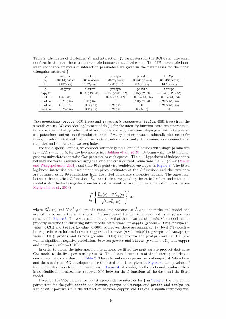
Table 2: Estimates of clustering, ψ, and interaction, ξ, parameters for the BCI data. The smallnumbers in the parentheses are parametric bootstrap standard errors. The 95% parametric boot-strap confidence intervals of interaction parameters are given in the parentheses for the uppertriangular entries of ξ.
ψ cappfr hirttr protpa protte tet2pa
κi .00114(.00033) .00097(.00048) .00057(.00036) .00167(.00048) .00046(.00026)
ωi 7.87(1.04) 11.22(1.84) 12.01(3.20) 5.56(1.93) 14.50(2.27)
ξ cappfr hirttr protpa protte tet2pa
cappfr 0 0.33∗(.13, .43) −0.21(-0.43, .07) 0.15(-.07, .32) −0.24∗(-.45, -.07)
hirttr 0.33(.08) 0 0.07(-.12, .27) −0.06(-.23, .16) −0.12(-.31, .06)
protpa −0.21(.13) 0.07(.10) 0 0.20(-.02, .47) 0.25∗(.02, .46)
protte 0.15(.10) −0.06(.10) 0.20(.13) 0 0.23∗(.02, .43)
tet2pa −0.24(.10) −0.12(.10) 0.25(.11) 0.23(.10) 0
tium tenuifolium (protte, 3091 trees) and Tetragastris panamensis (tet2pa, 4961 trees) from theseventh census. We consider log-linear models (1) for the intensity functions with ten environmen-tal covariates including interpolated soil copper content, elevation, slope gradient, interpolatedsoil potassium content, multi-resolution index of valley bottom flatness, mineralization needs fornitrogen, interpolated soil phosphorus content, interpolated soil pH, incoming mean annual solarradiation and topographic wetness index.
For the dispersal kernels, we consider variance gamma kernel functions with shape parametersνi = 1/2, i = 1, . . . , 5, for the five species (see Jalilian et al., 2013). To begin with, we fit inhomo-geneous univariate shot-noise Cox processes to each species. The null hypothesis of independencebetween species is investigated using the auto and cross centred L-functions, i.e. Lij(r)−r (Møllerand Waagepetersen, 2004), and their 95% pointwise confidence envelopes in Figure 3. The fittedlog-linear intensities are used in the empirical estimates of the L-functions and the envelopesare obtained using 99 simulations from the fitted univariate shot-noise models. The agreementbetween the empirical L-functions, Lij , and their corresponding theoretical values under the nullmodel is also checked using deviation tests with studentized scaling integral deviation measure (seeMyllymaki et al., 2013)
∫ t
0
Lij(r)− ELij(r)√
VarLij(r)
2
dr,
where ELij(r) and VarLij(r) are the mean and variance of Lij(r) under the null model andare estimated using the simulations. The p-values of the deviation tests with t = 75 are alsopresented in Figure 3. The p-values and plots show that the univariate shot-noise Cox model cannotproperly describe the clustering intra-specific correlations for cappfr (p-value=0.024), protpa (p-value=0.034) and tet2pa (p-value=0.008). Moreover, there are significant (at level 5%) positiveinter-specific correlations between cappfr and hirttr (p-value=0.001), protpa and tet2pa (p-value=0.001), protte and tet2pa (p-value=0.004) and protte and protpa (p-value=0.033) aswell as significant negative correlations between protte and hirttr (p-value 0.031) and cappfr
and tet2pa (p-value=0.010).In order to model the inter-specific interactions, we fitted the multivariate product-shot-noise
Cox model to the five species using t = 75. The obtained estimates of the clustering and depen-dence parameters are shown in Table 2. The auto and cross species centred empirical L-functionsand the associated 95% envelopes under the fitted model are given in Figure 4. The p-values ofthe related deviation tests are also shown in Figure 4. According to the plots and p-values, thereis no significant disagreement (at level 5%) between the L-functions of the data and the fittedmodel.
Based on the 95% parametric bootstrap confidence intervals for ξ in Table 2, the interactionparameters for the pairs cappfr and hirttr, protpa and tet2pa and protte and tet2pa aresignificantly positive while the interaction between cappfr and tet2pa is significantly negative.
10

0 20 40 60
01
23
4
r
cappfr (0.024)
empiricalsimulationPoissonenvelope
0 20 40 60
−1.
5−
0.5
0.5
1.5
r
hirttr & cappfr (0.001)
0 20 40 60
01
23
4
r
L inh
om, h
irttr
, hir
ttr(r)
hirttr (0.159)
0 20 40 60
−2
−1
01
2
r
protpa & cappfr (0.07)
0 20 40 60
−2
−1
01
2
r
L inh
om, p
rotp
a, h
irttr
(r)
protpa & hirttr (0.264)
0 20 40 60
02
46
8
r
L inh
om, p
rotp
a, p
rotp
a(r)
protpa (0.034)
0 20 40 60
−1.
5−
0.5
0.5
1.5
r
protte & cappfr (0.137)
0 20 40 60
−1
01
2
r
L inh
om, p
rotte
, hir
ttr(r)
protte & hirttr (0.031)
0 20 40 60
−2
−1
01
23
r
L inh
om, p
rotte
, pro
tpa(
r)
protte & protpa (0.033)
0 20 40 60
−2
01
23
4
r
L inh
om, p
rotte
, pro
tte(r)
protte (0.483)
0 20 40 60
−1.
5−
0.5
0.5
1.5
tet2pa & cappfr (0.01)
0 20 40 60
−1.
5−
0.5
0.5
1.5
L inh
om, t
et2p
a, h
irttr
(r)
tet2pa & hirttr (0.055)
0 20 40 60
−2
−1
01
2
L inh
om, t
et2p
a, p
rotp
a(r)
tet2pa & protpa (0.001)
0 20 40 60
−1
01
2
L inh
om, t
et2p
a, p
rotte
(r)
tet2pa & protte (0.004)
0 20 40 60
01
23
45
6
L inh
om, t
et2p
a, te
t2pa
(r)
tet2pa (0.008)
Figure 3: Auto and cross L(r) − r functions for five species in the BCI dataset along with 95%envelopes under the null model of independent species. The p-values of corresponding deviationtests are given in the parenthesis.
These four significant ξij parameters correspond directly to species pairs (i, j) with deviationsfrom the null model of independence. For the pair hirttr and protte, the deviation test wassignificant at the 5% level but the corresponding estimated ξhirttr,protte is just -0.06 with a boot-strap confidence interval of (−0.23, 0.16). This may seem as a contradiction. However, this reflectsthe property of our model that negative interactions between two species can be generated frommixed negative and positive interactions with a third species. For instance, the significantly neg-ative estimated ξcappfr,tet2pa and the significantly positive estimated ξhirttr,cappfr and ξtet2pa,prottegenerate negative interactions between hirttr and protte, see Figure 5. Also, for the pair protpaand protte the deviation test was significant at the 5% level but the bootstrap confidence inter-val of (−0.02, 0.47) for ξprotpa,protte contains zero. In this case, the positive interaction betweenprotpa and protte is due to that both of these species have significantly positive interactionswith tet2pa. Moreover, interactions between one species and another species further generatesintra-species clustering interactions for each species. Extra intra-specific clustering for cappfr
and tet2pa is thus resulting from inter-species repulsion between these species as reflected by thesignificantly negative estimated value of ξcappfr,tet2pa. This explains the better fit of intra-speciesclustering for these species by the multivariate model compared with the univariate models.
11

0 20 40 60
−5
05
10
r
cappfr (0.625)
empiricalsimulationPoissonenvelope
0 20 40 60
−5
05
r
hirttr & cappfr (0.797)
0 20 40 60
−5
05
10
r
L inh
om, h
irttr
, hir
ttr(r)
hirttr (0.833)
0 20 40 60
−6
−4
−2
02
4
r
protpa & cappfr (0.96)
0 20 40 60
−4
02
46
8
r
L inh
om, p
rotp
a, h
irttr
(r)
protpa & hirttr (0.817)
0 20 40 60
−5
05
10
r
L inh
om, p
rotp
a, p
rotp
a(r)
protpa (0.53)
0 20 40 60
−4
−2
02
4
r
protte & cappfr (0.801)
0 20 40 60
−6
−2
02
46
r
L inh
om, p
rotte
, hir
ttr(r)
protte & hirttr (0.502)
0 20 40 60
−6
−2
02
46
8
r
L inh
om, p
rotte
, pro
tpa(
r)
protte & protpa (0.721)
0 20 40 60
−4
02
46
8
r
L inh
om, p
rotte
, pro
tte(r)
protte (0.781)
0 20 40 60
−6
−4
−2
02
4
tet2pa & cappfr (0.781)
0 20 40 60
−6
−2
02
46
L inh
om, t
et2p
a, h
irttr
(r)
tet2pa & hirttr (0.55)
0 20 40 60
−5
05
L inh
om, t
et2p
a, p
rotp
a(r)
tet2pa & protpa (0.757)
0 20 40 60
−6
−2
02
46
8
L inh
om, t
et2p
a, p
rotte
(r)
tet2pa & protte (0.582)
0 20 40 60
−5
05
1015
L inh
om, t
et2p
a, te
t2pa
(r)
tet2pa (0.474)
Figure 4: Auto and cross L(r) − r functions for five species in the BCI dataset along with 95%envelopes under the fitted model. The p-values of the corresponding deviation tests are given inthe parenthesis.
cappfr protpahirttr tet2paprotte
-0.24
0.33 0.23
0.25
Figure 5: Significant inter-specific interaction parameters among BCI species.
12
6 Discussion
In this paper, we introduced a new multivariate product-shot-noise Cox process for modeling mul-tispecies spatial point patterns with clustering intra-specific interactions and positive or negativeinter-specific interactions. The model allows for asymmetric interactions where one species e.g.repels another but not vice versa and the null model of independent shot-noise Cox components(no inter-specific interactions) is a special case. Simulations of the model can therefore be used toinvestigate biological hypotheses about modes of species coexistence. The second-order propertiesof the model are easy to study since the auto and cross pair correlation functions have closed andtractable forms.
Parameters were estimated using a variant of second-order composite likelihood based on thecross pair correlation functions. A symmetry constraint was imposed on the parameters for reasonsof identifiability. However, even with the symmetry constraints we obtained a good fit of the multi-species point pattern data set being considered.
To explore the full potential of the model, research is needed to obtain more efficient methodsfor parameter estimation. Such methods could include maximum likelihood estimation imple-mented using Markov chain Monte Carlo or perhaps composite likelihood based on higher ordermoments. Both of these alternatives are computationally very challenging.
With the current estimation approach it is not feasible to model simultaneously all of thehundreds of species appearing in tropical rain forests. We therefore need to restrict attention e.g.to more abundant species. Also a preliminary coarse grouping of species based on species familiescould be considered. In temperate forests much fewer species occur and the model can be appliedwithout preprocessing of data.
Acknowledgements
We thank the Editor, the Associate Editor and the referee for their constructive and helpfulcomments.
Abdollah Jalilian and Rasmus Waagepetersens research was supported by the Danish Natu-ral Science Research Council, grant 09-072331 ‘Point process modelling and statistical inference’,Danish Council for Independent Research Natural Sciences, Grant 12-124675, ‘Mathematicaland Statistical Analysis of Spatial Data’, and by Centre for Stochastic Geometry and AdvancedBioimaging, funded by a grant from the Villum Foundation. Yongtao Guans research was sup-ported by NSF grant DMS-0845368, by NIH grant 1R01DA029081-01A1 and by the VELUXVisiting Professor Programme. Jorge Mateus research was supported by grants P1-1B2012-52 andMTM2013-43917-P.
The BCI forest dynamics research project was made possible by National Science Founda-tion grants to Stephen P. Hubbell: DEB-0640386, DEB-0425651, DEB-0346488, DEB-0129874,DEB-00753102, DEB-9909347, DEB-9615226, DEB-9615226, DEB-9405933, DEB-9221033, DEB-9100058, DEB-8906869, DEB-8605042, DEB-8206992, DEB-7922197, support from the Center forTropical Forest Science, the Smithsonian Tropical Research Institute, the John D. and CatherineT. MacArthur Foundation, the Mellon Foundation, the Small World Institute Fund, and numerousprivate individuals, and through the hard work of over 100 people from 10 countries over the pasttwo decades. The plot project is part the Center for Tropical Forest Science, a global network oflarge-scale demographic tree plots.
The BCI soils data set were collected and analyzed by J. Dalling, R. John, K. Harms, R. Stallardand J. Yavitt with support from NSF DEB021104, 021115, 0212284, 0212818 and OISE 0314581,STRI and CTFS. Paolo Segre and Juan Di Trani provided assistance in the field. The topographiccovariates were computed in SAGA GIS by Tomislav Hengl (http://spatial-analyst.net/).
Supplementary Materials
A simulation study is available with this paper in the supplementary material at the Biometricswebsite on Wiley Online Library.
13

References
Baddeley, A. and Turner, R. (2005). spatstat: an R package for analyzing spatial point patterns.Journal of Statistical Software 12, 1–42. URL: www.jstatsoft.org, ISSN: 1548-7660. 7
Baddeley, A. J., Møller, J., and Waagepetersen, R. (2000). Non- and semi-parametric estimationof interaction in inhomogeneous point patterns. Statistica Neerlandica 54, 329–350. 1
Brix, A. and Møller, J. (2001). Space-time multi type log Gaussian Cox processes with a view tomodelling weeds. Scandinavian Journal of Statistics 28, 471–488. 2
Comas, C. and Mateu, J. (2007). Modelling forest dynamics: a perspective from point processmethods. Biometrical journal 49, 176–196. 1
Condit, R. (1998). Tropical Forest Census Plots. Springer-Verlag and R. G. Landes Company,Berlin, Germany and Georgetown, Texas. 9
Daley, D. and Vere-Jones, D. (2003). An Introduction to the Theory of Point Processes. Vol. 1:Elementary Theory and Methods. Springer, New York, 2 edition. 7
Daley, D. and Vere-Jones, D. (2008). An Introduction to the Theory of Point Processes. Vol. 2:General Theory and Structure. Springer, New York, 2 edition. 16
Diggle, P. J. and Milne, R. K. (1983). Bivariate Cox processes: some models for bivariate spatialpoint patterns. Journal of the Royal Statistical Society, Series B 45, 11–21. 2
Grabarnik, P. and Sarkka, A. (2009). Modelling the spatial structure of forest stands by mul-tivariate point processes with hierarchical interactions. Ecological Modelling 220, 1232–1240.2
Guan, Y. (2006). A composite likelihood approach in fitting spatial point process models. Journalof the American Statistical Association 101, 1502–1512. 7, 8
Harkness, R. D. and Isham, V. (1983). A bivariate spatial point pattern of ants’ nests. AppliedStatistics 32, 293–303. 2
Hellmund, G., Prokesova, M., and Jensen, E. B. V. (2008). Levy-based Cox point processes.Advances in Applied Probability pages 603–629. 4
Hubbell, S. P., Condit, R., and Foster, R. B. (2005). Barro Colorado forest census plot data, URL:https://ctfs.arnarb.harvard.edu/webatlas/datasets/bci. 9
Hubbell, S. P., Foster, R. B., O’Brien, S. T., Harms, K. E., Condit, R., Wechsler, B., Wright, S. J.,and Loo de Lao, S. (1999). Light gap disturbances, recruitment limitation, and tree diversityin a neotropical forest. Science 283, 554–557. 9
Illian, J. and Burslem, D. (2007). Contributions of spatial point process modelling to biodiversitytheory. Journal de la Societe Francaise de Statistique 148, 9–29. 1
Illian, J., Penttinen, A., Stoyan, H., and Stoyan, D. (2008). Statistical Analysis and Modelling ofSpatial Point Patterns. Wiley, London. 3
Jalilian, A., Guan, Y., and Waagepetersen, R. (2013). Decomposition of variance for spatial Coxprocesses. Scandinavian Journal of Statistics 40, 119–137. 3, 9, 10
Law, R., Illian, J., Burslem, D. F., Gratzer, G., Gunatilleke, C., and Gunatilleke, I. (2009). Eco-logical information from spatial patterns of plants: insights from point process theory. Journalof Ecology 97, 616–628. 1
14

Liang, S., Carlin, B. P., and Gelfand, A. E. (2009). Analysis of minnesota colon and rectumcancer point patterns with spatial and nonspatial covariate information. The annals of appliedstatistics 3, 943–962. 2
Lieshout, M. N. M. V. and Baddeley, A. (1999). Indices of dependence between types in multi-variate point patterns. Scandinavian Journal of Statistics 26, 511–532. 1
Luo, Z. R., Ming, J. Y., Chen, D. L., Wu, Y. G., and Ding, B. Y. (2012). Spatial associations oftree species in a subtropical evergreen broad-leaved forest. Journal of Plant Ecology 5, 346–355.1
Matern, B. (1986). Spatial Variation. Lecture Notes in Statistics 36, Springer-Verlag, Berlin. 3
Møller, J. (2003). Shot noise Cox processes. Advances in Applied Probability pages 614–640. 3
Møller, J., Syversveen, A. R., and Waagepetersen, R. P. (1998). Log Gaussian Cox processes.Scandinavian Journal of Statistics 25, 451–482. 2, 3
Møller, J. and Waagepetersen, R. P. (2004). Statistical inference and simulation for spatial pointprocesses. Chapman and Hall/CRC, Boca Raton. 2, 3, 7, 10, 16, 17
Myllymaki, M., Grabarnik, P., Seijo, H., and Stoyan, D. (2013). Deviation test construction andpower comparison for marked spatial point patterns. arXiv preprint arXiv:1306.1028 . 10
Nathaniel Holland, J. and DeAngelis, D. L. (2009). Consumer-resource theory predicts dynamictransitions between outcomes of interspecific interactions. Ecology Letters 12, 1357–1366. 1
Picard, N., Bar-Hen, A., Mortier, F., and Chadœuf, J. (2009a). The multi-scale marked area-interaction point process: A model for the spatial pattern of trees. Scandinavian Journal ofStatistics 36, 23–41. 2
Picard, N., Bar-Hen, A., Mortier, F., and Chadœuf, J. (2009b). Understanding the dynamics ofan undisturbed tropical rain forest from the spatial pattern of trees. Journal of Ecology 97,97–108. 1
Prokesova, M. and Jensen, E. B. (2013). Asymptotic Palm likelihood theory for stationary pointprocesses. Annals of the Institude of Statistical Mathematics 65, 387–412. 8
Renner, I. W. and Warton, D. I. (2013). Equivalence of MAXENT and Poisson point processmodels for species distribution modeling in ecology. Biometrics . 2
Stoyan, D. and Penttinen, A. (2000). Recent applications of point process methods in forestrystatistics. Statistical Science 15, 61–78. 1
Waagepetersen, R. and Guan, Y. (2009). Two-step estimation for inhomogeneous spatial pointprocesses. Journal of the Royal Statistical Society: Series B (Statistical Methodology) 71, 685–702. 1, 2, 7, 8, 9
Waagepetersen, R. P. (2007). An estimating function approach to inference for inhomogeneousneyman–scott processes. Biometrics 63, 252–258. 1, 2, 7, 9
Wiegand, T., Gunatilleke, S., and Gunatilleke, N. (2007). Species associations in a heterogeneousSri Lankan dipterocarp forest. The American Naturalist 170, E77–E95. 1
Wootton, J. T. and Emmerson, M. (2005). Measurement of interaction strength in nature. AnnualReview of Ecology, Evolution, and Systematics 36, 419–444. 1
15

A
A.1 Derivations
Let Φ be a stationary Poisson process with intensity κ > 0. Then for every function f : R2 →(−1,∞) where (Daley and Vere-Jones, 2008, p. 60)
∫
R2
∣∣∣ log{
1 + f(u)}∣∣∣du <∞,
the expectation of the random product∏v∈Φ
[1 − f(v)
]exists and (Møller and Waagepetersen,
2004, Prop. 3.3)
E∏
v∈Φ
{1 + f(v)
}= exp
{κ
∫
R2
f(v)dv
}.
Let k be a translation invariant (probability) kernel function on R2, i.e. k(u, v) = k(u − v), andfor every u ∈ R2, define fu(v) = k(v − u)/k(0). For ξ > 0
∣∣∣ log{
1 + ξfu(v)}∣∣∣ = log
{1 + ξfu(v)
}≤ ξfu(v)
and for −1 < ξ < 0
∣∣∣ log{
1 + ξfu(v)}∣∣∣ = − log
{1− |ξ|fu(v)
}= log
{1 +
|ξ|fu(v)
1− |ξ|fu(v)
}
≤ |ξ|fu(v)
1− |ξ|fu(v)≤ |ξ|fu(v)
1− |ξ| supv∈R2 fu(v).
If the kernel function k is bounded, i.e. supv∈R2 k(v) < ∞, it follows that for every u ∈ R2 and
ξ ∈ (−1,∞),∫R2
∣∣∣ log{
1 + ξfu(v)}∣∣∣dv <∞. Thus
E∏
v∈Φ
{1 + ξ
k(u− v)
k(0)
}= exp
(κξ
k(0)
∫
R2
k(v)dv
)= exp
(κξ
k(0)
).
The Gaussian and Cauchy kernels in Table 1 are bounded while the variance gamma kernel isbounded when ν > 0.
Therefore, the nonnegative random field
Eξ(u) = exp
(− κξ
k(0)
)∏
v∈Φ
{1 + ξ
k(u− v)
k(0)
},
has expectation EEξ(u) ≡ 1. Moreover,
EEξ(u)Eξ′(u′) = exp
{−κ(ξ + ξ′)
k(0)
}E
[∏
v∈Φ
{1 + ξ
k(u− v)
k(0)
} ∏
v′∈Φ
{1 + ξ′
k(u′ − v′)k(0)
}]
= exp
{−κ(ξ + ξ′)
k(0)
}E∏
v∈Φ
[1 +
{ξk(u− v)
k(0)+ ξ′
k(u′ − v)
k(0)+ ξξ′
k(u− v)k(u′ − v)
k(0)2
}]
= exp
[−κ(ξ + ξ′)
k(0)+ κ
∫
R2
{ξk(u− v)
k(0)+ ξ′
k(u′ − v)
k(0)+ ξξ′
k(u− v)k(u′ − v)
k(0)2
}dv
]
= exp
(κξξ′
k(0)2
∫
R2
k(u− v)k(u′ − v)dv
).
16

Letting S(u) = 1κ
∑v∈Φ k(u− v), by an application of Slivnyak-Mecke’s theorem (see Møller and
Waagepetersen, 2004, Theo. 3.2),
ES(u)Eξ(u′) =
1
κexp
(− κξ
k(0)
)E
[{∑
v∈Φ
k(u− v)
}{∏
w∈Φ
(1 + ξ
k(u′ − w)
k(0)
)}]
=1
κexp
(− κξ
k(0)
)E∑
v∈Φ
k(u− v)
{1 + ξ
k(u′ − v)
k(0)
} ∏
w∈Φ\{v}
{1 + ξ
k(u′ − w)
k(0)
}
= exp
(− κξ
k(0)
)∫
R2
[k(u− v)
{1 + ξ
k(u′ − v)
k(0)
}E∏
w∈Φ
{1 + ξ
k(u′ − w)
k(0)
}]dv
=
∫
R2
k(u− v)
{1 + ξ
k(u′ − v)
k(0)
}dv
= 1 +ξ
k(0)
∫
R2
k(u− v)k(u′ − v)dv.
Combining these results with (2) and (8) we obtain (9) and (10).
17