Embed Size (px)
Citation preview

Research report
MA12-01
University of Leicester
Department of Mathematics
2012

THERMODYNAMIC TREE: THE SPACE OF ADMISSIBLE PATHS
ALEXANDER N. GORBAN∗
Abstract. Is a spontaneous transition from a state x to a state y allowed by thermodynamics?Such a question arises often in chemical thermodynamics and kinetics. We ask the more formalquestion: is there a continuous path between these states, along which the conservation laws hold, theconcentrations remain non-negative and the relevant thermodynamic potential G (Gibbs energy, forexample) monotonically decreases? The obvious necessary condition, G(x) ≥ G(y), is not sufficient,and we construct the necessary and sufficient conditions. For example, it is impossible to overstepthe equilibrium in 1-dimensional (1D) systems (with n components and n−1 conservation laws). Thesystem cannot come from a state x to a state y if they are on the opposite sides of the equilibrium evenif G(x) > G(y). We find the general multidimensional analogue of this 1D rule and constructivelysolve the problem of the thermodynamically admissible transitions.
We study dynamical systems, which are given in a positively invariant convex polyhedron D andhave a convex Lyapunov function G. An admissible path is a continuous curve in D along whichG does not increase. For x, y ∈ D, x % y (x precedes y) if there exists an admissible path from xto y and x ∼ y if x % y and y % x. The tree of G in D is a quotient space D/ ∼. We provide analgorithm for the construction of this tree. In this algorithm, the restriction of G onto the 1-skeletonof D (the union of edges) is used. The problem of existence of admissible paths between states issolved constructively. The regions attainable by the admissible paths are described.
Key words. Lyapunov function, convex polyhedron, attainability, tree of function, entropy, freeenergy
AMS subject classifications. 37A60, 52A41, 80A30, 90C25
1. Introduction.
1.1. Motivation, ideas and a simple example. “Applied dynamical sys-tems” are models of real systems. The available information about the real systemsis incomplete and uncertainties of various types are encountered in the modeling. Of-ten, we view them as errors: errors in the model structure, errors in coefficients, inthe state observation and many others. Nevertheless, there is an order in this worldof errors: some information is more reliable, we trust in some structures more andeven respect them as laws. Some other data are less reliable. There is an hierarchyof reliability, our knowledge and beliefs (described, for example by R. Peierls [53] formodel making in physics). Extracting as many consequences from the more reliabledata either without or before use of the less reliable information is a task which arisesnaturally.
In our paper, we study dynamical systems with a strictly convex Lyapunov func-tion G defined in a positively invariant convex polyhedron D. For them, we analyzethe admissible paths, along which G decreases monotonically, and find the states thatare attainable from the given initial state along the admissible paths. The main areaof applications of these systems is chemical kinetics and thermodynamics. The mo-tivation of our research comes from the hierarchy of reliability of the information inthese applications.
Let us discuss the motivation in more detail. In chemical kinetics, we can rankthe information in the following way. First of all, the list of reagents and conservationlaws should be known. Let the reagents be A1, A2, . . . , An. The non-negative realvariable Ni ≥ 0, the amount of Ai in the mixture, is defined for each reagent, and Nis the vector of composition with coordinates Ni. The conservation laws are presented
∗Department of Mathematics, University of Leicester, UK ([email protected]).
1
2 A. N. GORBAN
by the linear balance equations:
bi(N) =
n∑
j=1
ajiNj = const (i = 1, . . . ,m) . (1.1)
We assume that the linear functions bi(N) (i = 1, . . . ,m) are linearly independent.The list of the components together with the balance conditions (1.1) is the first
part of the information about the kinetic model. This determines the space of states,the polyhedronD defined by the balance equations (1.1) and the positivity inequalitiesNi ≥ 0. This is the background of kinetic models and any further development isless reliable. The polyhedron D is assumed to be bounded. This means that thereexist such coefficients λi that the linear combination
∑i λibi(N) has strictly positive
coefficients:∑
i λiaji > 0 for all j = 1, . . . , n.
The thermodynamic functions provide us with the second level of informationabout the kinetics. Thermodynamic potentials, such as the entropy, energy and freeenergy are known much better than the reaction rates and, at the same time, theygive us some information about the dynamics. For example, the entropy increases inisolated systems. The Gibbs free energy decreases in closed isothermal systems underconstant pressure, and the Helmholtz free energy decreases under constant volumeand temperature. Of course, knowledge of the Lyapunov functions gives us someinequalities for vector fields of the systems’ velocity but the values of these vectorfields remain unknown. If there are some external fluxes of energy or non-equilibriumsubstances then the thermodynamic potentials are not Lyapunov functions and thesystems do not relax to the thermodynamic equilibrium. Nevertheless, the inequalityof positivity of the entropy production persists and this gives us useful informationeven about the open systems. Some examples are given in [26, 28].
The next, third part of the information about kinetics is the reaction mechanism.It is presented in the form of the stoichiometric equations of the elementary reactions:
∑
i
αρiAi →∑
i
βρiAi , (1.2)
where ρ = 1, . . . ,m is the reaction number and the stoichiometric coefficients αρi, βρi(i = 1, . . . , n) are nonnegative integers.
A stoichiometric vector γρ of the reaction (1.2) is a n-dimensional vector withcoordinates γρi = βρi − αρi, that is, ‘gain minus loss’ in the ρth elementary reaction.
The concentration of Ai is an intensive variable ci = Ni/V , where V > 0 is thevolume. The vector c = N/V with coordinates ci is the vector of concentrations. Anon-negative intensive quantity, rρ, the reaction rate, corresponds to each reaction(1.2). The kinetic equations in the absence of external fluxes are
dN
dt= V
∑
ρ
rργρ . (1.3)
If the volume is not constant then equations for concentrations include V and havedifferent form.
For perfect systems and not so fast reactions the reaction rates are functions ofconcentrations and temperature given by the mass action law and by the generalizedArrhenius equation. A special relation between the kinetic constants is given by theprinciple of detailed balance: For each value of temperature T there exists a positive

THERMODYNAMIC TREE 3
equilibrium point where each reaction (1.2) is equilibrated with its reverse reaction.This principle was introduced for collisions by Boltzmann in 1872 [10]. Wegscheiderintroduced this principle for chemical kinetics in 1901 [67]. Einstein in 1916 used it inthe background for his quantum theory of emission and absorption of radiation [17].Later, it was used by Onsager in his famous work [51]. For a recent review see [30].
At the third level of reliability of information, we select the list of componentsand the balance conditions, find the thermodynamic potential, guess the reactionmechanism, accept the principle of detailed balance and believe that we know thekinetic law of elementary reactions. However, we still do not know the reaction rateconstants.
Finally, at the fourth level of available information, we find the reaction rateconstants and can analyze and solve the kinetic equations (1.3) or their extendedversion with the inclusion of external fluxes.
Of course, this ranking of the available information is conventional, to a cer-tain degree. For example, some reaction rate constants may be known even betterthan the list of intermediate reagents. Nevertheless, this hierarchy of the informationavailability, list of components – thermodynamic functions – reaction mechanism –reaction rate constants, reflects the real process of modelling and the stairs of availableinformation about a reaction kinetic system.
It seems very attractive to study the consequences of the information of eachlevel separately. These consequences can be also organized ‘stairwise’. We have thehierarchy of questions: how to find the consequences for the dynamics (i) from the listof components, (ii) from this list of components plus the thermodynamic functions ofthe mixture, and (iii) from the additional information about the reaction mechanism.
The answer to the first question is the description of the balance polyhedron D.The balance equations (1.1) together with the positivity conditions Ni ≥ 0 shouldbe supplemented by the description of all the faces. For each face, some Ni = 0 andwe have to specify which Ni have zero value. The list of the corresponding indicesi, for which Ni = 0 on the face, I = {i1, . . . , ik}, fully characterizes the face. Thisproblem of double description of the convex polyhedra [49, 14, 21] is well known inlinear programming.
The list of vertices [6] and edges with the corresponding indices is necessaryfor the thermodynamic analysis. This is the 1-skeleton of D. Algorithms for theconstruction of the 1-skeletons of balance polyhedra as functions of the balance valueswere described in detail in 1980 [26]. The related problem of double description forconvex cones is very important for the pathway analysis in systems biology [58, 22].
In this work, we use the 1-skeleton of D, but the main focus is on the second step,i.e. on the consequences of the given thermodynamic potentials. For closed systemsunder classical conditions, these potentials are the Lyapunov functions for the kineticequations. For example, for perfect systems we assume the mass action law. If theequilibrium concentrations c∗ are given, the system is closed and both temperatureand volume are constant then the function
G =∑
i
ci(ln(ci/c∗i )− 1) (1.4)
is the Lyapunov function; it should not increase in time. The function G is pro-portional to the free energy F = RTG + const (for detailed information about theLyapunov functions for kinetic equations under classical conditions see the textbook[68] or the recent paper [33]).

4 A. N. GORBAN
A1
A2 A3
c*
c1=c3=1/2
G(c)=g0
G(c)>g0
G(c)<g0
c1=c2=1/2
c1≈0.773
b)
c
c1
A1
A2 A3
a)
c) G
G(c*)
g0
gmax
c*
A1 A2 A3
A1
A2 A3
c*
d)
c
c'
c*'
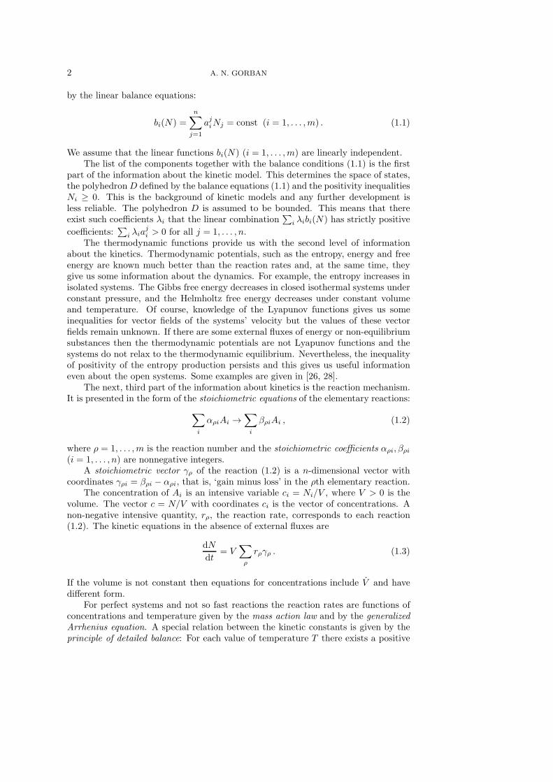
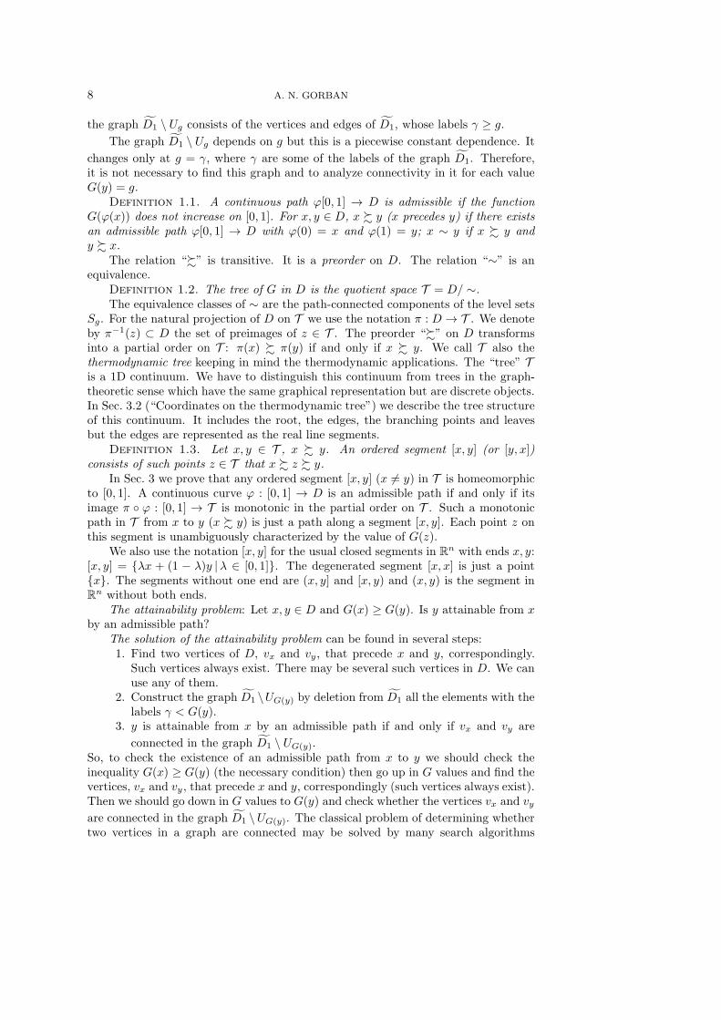
Fig. 1.1. The balance simplex (a), the levels of the Lyapunov function (b) and the thermody-namic tree (c) for the simple system of three components, A1, A2, A3. Algorithm for finding a vertexv % c (d).
If we know the Lyapunov function G then we have the necessary conditions forthe possibility of transition from the vector of concentrations c to c′ during the non-stationary reaction: G(c) ≥ G(c′) because the inequality G(c(t0)) ≥ G(c(t0+t)) holdsfor any time t ≥ 0.
The inequality G(c) ≥ G(c′) is necessary if we are to reach c′ from the initialstate c by a thermodynamically admissible path, but it is not sufficient because inaddition to this inequality there are some other necessary conditions. The simplestand most famous of them is: if D is one-dimensional (a segment) then the equilibriumc∗ divides this segment into two parts and both c(t0) and c(t0 + t) (t > 0) are alwayson the same side of the equilibrium.
In 1D systems the overstepping of the equilibrium is forbidden. It is impossibleto overstep a point in dimension one, but it is possible to circumvent a point inhigher dimensions. Nevertheless, in any dimension the inequality G(c) ≥ G(c′) is notsufficient if we are to reach c′ from the initial state c along an admissible path. Someadditional restrictions remain in the general case as well. A two-dimensional exampleis presented in Fig. 1.1. Let us consider the mixture of three components, A1,2,3 withthe only conservation law c1 + c2 + c3 = b (we take for illustration b = 1) and theequidistribution in equilibrium c∗1 = c∗2 = c∗3 = 1/3. The balance polyhedron is thetriangle (Fig. 1.1a). In Fig. 1.1b the level sets of
G =3∑
i=1
ci(ln(3ci)− 1)
are presented. This function achieves its minimum at equilibrium, G(c∗) = −1. Onthe edges, the function G achieves its conditional minimum, g0, in the middles, andg0 = ln(3/2)− 1. G reaches its maximal value, gmax = ln 3− 1, at the vertices.
If G(c∗) < g ≤ g0 then the level set G(c) = g is connected. If g0 < g ≤ gmax then
THERMODYNAMIC TREE 5
the corresponding level set G(c) = g consists of three components (Fig. 1.1b). Thecritical value is g = g0. The critical level G(c) = g0 consists of three arcs. Each arcconnects two middles of the edges and divides D in two sets. One of them is convexand includes two vertices, the other includes the remaining vertex.
A thermodynamically admissible path is a continuous curve along which G doesnot increase. Therefore, such a path cannot intersect these arcs ‘from inside’, i.e.from values G(c) ≤ g0 to bigger values, G(c) > g0. For example, if an admissible pathstarts from the state with 100% of A2, then it cannot intersect the arc that separatesthe vertex with 100% A1 from two other vertices. Therefore, any vertex cannot bereached from another one and if we start from 100% of A2 then the reaction cannotovercome the threshold ∼77.3% of A1, that is the maximum of c1 on the correspondingarc (Fig. 1.1b). This is an example of the 2D analogue of the 1D prohibition ofoverstepping of equilibrium.
For x, y ∈ D, x % y (x precedes y) if there exists a thermodynamically admissiblepath from x to y, and x ∼ y if x % y and y % x. The equivalence classes withrespect to x ∼ y in D are the connected components of the level sets G(c) = g.The quotient space T = D/ ∼ is the space of these connected components. For thecanonical projection we use the standard notation π : D → T . This is the tree of theconnected components of the level sets of G. (Here “tree” stands for a one dimensionalcontinuum, a sort of dendrites [13], and not for a tree in the sense of the graph theory.)
If x ∼ y then G(x) = G(y). Therefore, we can define the function G on the tree:G(π(c)) = G(c). It is convenient to draw this tree on the plane with the verticalcoordinate g = G(x) (Fig. 1.1c). The equilibrium c∗ corresponds to a root of thistree, π(c∗). If G(c∗) < g ≤ g0 then the level set G(c) = g corresponds to one point onthe tree. The level G(c) = g0 corresponds to the branching point, and each connectedcomponent of the level sets G(c) = g with g0 < g ≤ gmax corresponds to a separatepoint on the tree. The terminal points (“leaves” with g > g0) of the tree correspondto the vertices of D.
An ordered segment [x, y] or [y, x] (x % y) on the tree T consists of such points zthat x % z % y. A continuous curve ϕ : [0, 1] → D is an admissible path if and only ifits image π◦ϕ : [0, 1] → T is a path that goes monotonically down in the coordinate g.Such a monotonic path in T from a point x to the root is just a segment [x, π(c∗)]. Onthis segment, each point y is unambiguously characterized by g = G(y). Therefore,if for c ∈ D we know the value G(c) and a vertex v % c, then we can unambiguouslydescribe the image of c on the tree: π(c) is the point on the segment [π(v), π(c∗)] withthe given value of G, g = G(c).
We can find a vertex v % c by a chain of central projections: the first step is thecentral projection of c onto the border of D with center c∗. The result is the point c′
on a face (in Fig. 1.1d this is the point c′ on an edge). The second step is the centralprojection of the point c′ onto the border of the face with the center at the partialequilibrium c∗′ (that is, the minimizer of G on the face) and so on (Fig. 1.1d). If theprojection on a face is the partial equilibrium then for any vertices v of the face v % c.In particular, if the face is a vertex v then v % c. For a simple example presented inFig. 1.1d this is the vertex A1.
In this paper, we extend these ideas and observations to any dynamical system,which is given in a positively invariant convex polyhedron and has there a strictlyconvex Lyapunov function. The class of chemical kinetic equations for closed systemsprovides us standard and practically important examples of the systems of this class.
6 A. N. GORBAN
1.2. A bit of history. It seems attractive to use an attainable region insteadof the single trajectory in situations with incomplete information or with informationwith different levels of reliability. Such situations are typical in many areas of scienceand engineering. For example, the theory for the continuous–time Markov chain ispresented in [2, 27] and for the discrete–time Markov chains in [3].
Perhaps, the first celebrated example of this approach was developed in biologicalkinetics. In 1936, A.N. Kolmogorov [40] studied the dynamics of interacting popula-tions of prey (x) and predator (y) in the general form:
x = xS(x, y), y = yW (x, y)
under monotonicity conditions: ∂S(x, y)/∂y < 0, ∂W (x, y)/∂y < 0. The zero iso-clines, given by equations S(x, y) = 0 or W (x, y) = 0, are graphs of two functionsy(x). These isoclines divide the phase space into compartments with curvilinearborders. The geometry of the intersection of the zero isoclines, together with somemonotonicity conditions, contain important information about the system dynamicsthat we can find [40] without exact knowledge of the kinetic equations. This approachto population dynamics was applied to various problems [45, 7]. The impact of thiswork on population dynamics was analyzed in the review [62].
In 1964, Horn proposed to analyze the attainable regions for chemical reactors[36]. This approach became popular in chemical engineering. It was applied to theoptimization of steady flow reactors [23], to batch reactor optimization without knowl-edge of detailed kinetics [19], and for optimization of the reactor structure [34]. Ananalysis of attainable regions is recognized as a special geometric approach to reactoroptimization [18] and as a crucially important part of the new paradigm of chemicalengineering [35].
Many particular applications were developed, from polymerization [63] to particlebreakage in a ball mill [47] and hydraulic systems [28]. Mathematical methods for thestudy of attainable regions vary from Pontryagin’s maximum principle [46] to linearprogramming [38], the Shrink-Wrap algorithm [43], and convex analysis. In 1979 itwas demonstrated how to utilize the knowledge about partial equilibria of elementaryprocesses to construct the attainable regions [24]. The attainable regions significantlydepend on the reaction mechanism and it is possible to use them for the discriminationof mechanisms [29].
Thermodynamic data are more robust than the reaction mechanism. Hence, thereare two types of attainable regions. The first is the thermodynamic one, which usethe linear restrictions and the thermodynamic functions [25]. The second is generatedby thermodynamics and stoichiometric equations of elementary steps (but withoutreaction rates) [24, 31]. R. Shinnar and other authors [61] rediscovered this approach.There was even an open discussion about priority [9].
Some particular classes of kinetic systems have rich families of the Lyapunovfunctions. Krambeck [41] studied attainable regions for linear systems and the l1Lyapunov norm instead of the entropy. Already simple examples demonstrate thatthe sets of distributions which are accessible from a given initial distribution by linearkinetic systems (Markov processes) with a given equilibrium are, in general, non-convex polytopes [24, 27, 70]. The geometric approach to attainability was developedfor all the thermodynamic potentials and for open systems as well [26]. Partial resultsfor chemical kinetics and some other engineering systems are summarized in [68, 28].
The tree of the level set components for differentiable functions was introduces inthe middle of the 20 century by Adelson-Velskii and Kronrod [1, 42] and Reeb [56].
THERMODYNAMIC TREE 7
Sometimes these trees are called the Reeb trees [20] but from the historical point ofview it may be better to call them the Adelson-Velskii – Kronrod – Reeb (or AKR)trees. These trees were essentially used by Kolmogorov and Arnold [4] in solution ofthe Hilbert’s superposition problem (the ideas, their relations to dynamical systemsand role in the Arnold’s scientific life are discussed in his lecture [5]).
The general Reeb graph can be defined for any topological space X and realfunction f on it. It is the quotient space of X by the equivalence relation “∼” definedby x ∼ y holds if and only if f(x) = f(y) and x, y are in the same connectedcomponent of f−1(f(x)). Of course, this “graph” is again not a discrete object fromthe graph theory but a topological space. It has application in differential topology(Morse theory [48]), in topological shape analysis and visualization [20, 39], in dataanalysis [64] and in asymptotic analysis of fluid dynamics [44, 59]. The books [20, 39]include many illustration of the Reeb graphs. The efficient mesh-based methods forthe computation of the graphs of level set components are developed for general scalarfields on 2- and 3-dimensional manifolds [16].
Some time ago the tree of entropy in the balance polyhedra was rediscovered as anadequate tool for representation of the attainable regions in chemical thermodynamics[25, 26]. It was applied to analysis of various real systems [37, 69]. Nevertheless, someof the mathematical backgrounds of this approach were delayed in development andpublications. Now, the thermodynamically attainable regions are in extensive use inchemical engineering and beyond [18, 19, 23, 28, 34, 35, 36, 37, 38, 41, 43, 46, 47, 60, 61,63, 69]. In this paper we aim to provide the complete mathematical background for theanalysis of the thermodynamically attainable regions. For this purpose, we constructthe trees of strictly convex functions in a convex polyhedron. This problem allows ageneral meshless solution in higher dimensions because topological and geometricalsimplicity (the domain D is a convex polyhedron and the function G is strictly convexin D). In this paper, we present this solution in detail.
1.3. The problem of attainability and its solution. Let us formulate pre-cisely the problem of attainability and its solution before the exposition of all technicaldetails and proofs. Our results are applicable to any dynamical system that obeys acontinuous strictly convex Lyapunov function in a positively invariant convex polyhe-dron. The situations with uncertainty, when the specific dynamical system is not givenwith an appropriate accuracy but the Lyapunov function is known, give a natural areaof application of these results.
Here and below, D is a convex polyhedron in Rn, D0 consists of the vertices ofD, D1 is the union of the closed edges of D, that is, the 1-skeleton of D, and D1 isthe graph whose vertices correspond to the vertices of D and edges correspond to theedges of D, (the graph of the 1-skeleton) of D. We use the same notations for vertices
and edges of D and D1.Let a real continuous function G be given in D. We assume that G is strictly
convex in D [57]. Let x∗ be the minimizer of G in D and let g∗ = G(x∗) be thecorresponding minimal value.
The level set Sg = {x ∈ D |G(x) = g} is closed and the sublevel set Ug = {x ∈D |G(x) < g} is open in D (i.e. it is the intersection of an open subset of Rn withD).
Let us transform D1 into a labeled graph. Each vertex v ∈ D0 is labeled by thevalue γv = G(v) and each edge e = [v, w] ⊂ D1 is labeled by the minimal value of G on
the segment [v, w] ⊂ D, ge = min[v,w]G(x). The vertices and edges of D1 are labeledby the same numbers as the correspondent vertices and edges of D1. By definition,
8 A. N. GORBAN
the graph D1 \ Ug consists of the vertices and edges of D1, whose labels γ ≥ g.
The graph D1 \ Ug depends on g but this is a piecewise constant dependence. It
changes only at g = γ, where γ are some of the labels of the graph D1. Therefore,it is not necessary to find this graph and to analyze connectivity in it for each valueG(y) = g.
Definition 1.1. A continuous path ϕ[0, 1] → D is admissible if the functionG(ϕ(x)) does not increase on [0, 1]. For x, y ∈ D, x % y (x precedes y) if there existsan admissible path ϕ[0, 1] → D with ϕ(0) = x and ϕ(1) = y; x ∼ y if x % y andy % x.
The relation “%” is transitive. It is a preorder on D. The relation “∼” is anequivalence.
Definition 1.2. The tree of G in D is the quotient space T = D/ ∼.The equivalence classes of ∼ are the path-connected components of the level sets
Sg. For the natural projection of D on T we use the notation π : D → T . We denoteby π−1(z) ⊂ D the set of preimages of z ∈ T . The preorder “%” on D transformsinto a partial order on T : π(x) % π(y) if and only if x % y. We call T also thethermodynamic tree keeping in mind the thermodynamic applications. The “tree” Tis a 1D continuum. We have to distinguish this continuum from trees in the graph-theoretic sense which have the same graphical representation but are discrete objects.In Sec. 3.2 (“Coordinates on the thermodynamic tree”) we describe the tree structureof this continuum. It includes the root, the edges, the branching points and leavesbut the edges are represented as the real line segments.
Definition 1.3. Let x, y ∈ T , x % y. An ordered segment [x, y] (or [y, x])consists of such points z ∈ T that x % z % y.
In Sec. 3 we prove that any ordered segment [x, y] (x 6= y) in T is homeomorphicto [0, 1]. A continuous curve ϕ : [0, 1] → D is an admissible path if and only if itsimage π ◦ ϕ : [0, 1] → T is monotonic in the partial order on T . Such a monotonicpath in T from x to y (x % y) is just a path along a segment [x, y]. Each point z onthis segment is unambiguously characterized by the value of G(z).
We also use the notation [x, y] for the usual closed segments in Rn with ends x, y:[x, y] = {λx + (1 − λ)y |λ ∈ [0, 1]}. The degenerated segment [x, x] is just a point{x}. The segments without one end are (x, y] and [x, y) and (x, y) is the segment inRn without both ends.
The attainability problem: Let x, y ∈ D and G(x) ≥ G(y). Is y attainable from xby an admissible path?
The solution of the attainability problem can be found in several steps:1. Find two vertices of D, vx and vy, that precede x and y, correspondingly.
Such vertices always exist. There may be several such vertices in D. We canuse any of them.
2. Construct the graph D1 \UG(y) by deletion from D1 all the elements with thelabels γ < G(y).
3. y is attainable from x by an admissible path if and only if vx and vy are
connected in the graph D1 \ UG(y).So, to check the existence of an admissible path from x to y we should check theinequality G(x) ≥ G(y) (the necessary condition) then go up in G values and find thevertices, vx and vy , that precede x and y, correspondingly (such vertices always exist).Then we should go down in G values to G(y) and check whether the vertices vx and vyare connected in the graph D1 \UG(y). The classical problem of determining whethertwo vertices in a graph are connected may be solved by many search algorithms

THERMODYNAMIC TREE 9
[52, 50], for example, by the elementary breadth–first or depth–first search algorithms.The procedure “find a vertex vx ∈ D0 that precedes x ∈ D” can be implemented
as follows:1. If x = x∗ then any vertex v ∈ D0 precedes x.2. If x 6= x∗ then consider the ray rx = {x∗+λ(x−x∗) |λ ≥ 0}. The intersectionrx ∩D is a closed segment [x∗, x′]. We call x′ the central projection of x ontothe border of D with the center x∗; x′ % x.
3. The central projection x′ always belongs to an interior of a face D′ of D,0 ≤ dimD′ < dimD. If dimD′ > 0 then set x := x′, D := D′, x∗ :=argmin{G(z) | z ∈ D′} and go to step 1.
4. If dimD′ = 0 then it is a vertex v % x we are looking for.The dimension of the face decreases at each step, hence, after not more than dimD−1steps we will definitely obtain the desired vertex. A simple example is presented inFig. 1.1d.
The information about all connected components of D1 \ Ug for all values ofg is summarized in the tree of G in D, T (Definition 1.2). The tree T can bedescribed as follows (Theorem 3.3): it is the space of pairs (g,M), where g ∈
[minD G(x),maxD G(x)] andM is a connected component of D1 \Ug, with the partialorder relation: (g,M) % (g′,M ′) if g ≥ g′ and M ⊆ M ′. For x, y ∈ D, x % y if andonly if π(x) % π(y).
The tree T may be constructed gradually, by descending from the maximal valueof G, g = gmax (Sec. 3.3). At g = gmax, the graph D1 \ Ug consists of the isolatedvertices with the labels γ = gmax (generically, this is one vertex). Going down in
g, we add to D1 \ Ug the elements, vertices and edges, in descending order of theirlabels. After adding each element we record the changes in the connected componentsof D1 \ Ug.
For each point z ∈ T , z = (g,M), its preimage in D, π−1(g,M), may be describedby the equation G(x) = g supplemented by a set of linear inequalities. Computation-ally, these linear inequalities can be produced by a convex hull operation from a finiteset. This finite set is described explicitly in Sec. 3.4.
For each point z = (g,M) the set of all z′ = (g′,M ′) attainable by admissiblepaths from z has a simple description, g′ ≤ g, M ′ ⊇M .
The tree of G in D provides a workbench for the analysis of various questionsabout admissible paths. It allows us to reduce the n-dimensional problems in D tosome auxiliary questions about such 1D or even discrete objects as the tree T and thelabeled graph D1. For example, we use the thermodynamic tree to solve the followingproblem of attainable sets: For a given x ∈ D describe the set of all y - x by a systemof inequalities. For this purpose, we find the image of x in T , π(x), then define theset of all points attainable by admissible paths from π(x) in T and, finally, describethe preimage of this set in D by the system of inequalities (Sec. 3.4).
1.4. The structure of the paper. In Sec. 2, we present several auxiliary propo-sitions from convex geometry. We constructively describe the result of the cutting ofa convex polyhedron D by a convex set U : The description of the connected compo-nents of D \ U is reduced to the analysis of the 1D continuum D1 \ U , where D1 isthe 1-skeleton of D.
In Sec. 3, we construct the tree of level set components of a strictly convex functionG in the convex polyhedronD and study the properties of this tree. The main result ofthis section is the algorithm for construction of this tree (Sec. 3.3). This constructionis applied to the description of the attainable sets in Sec. 3.4. These sections include
10 A. N. GORBAN
some practical recipes and it is possible to read them independently, immediately afterIntroduction. Several examples of the thermodynamic trees for chemical systems arepresented in Sec. 4.
2. Cutting of a polyhedron D by a convex set U .
2.1. Connected components of D \ U and of D1 \ U . Let D be a convexpolyhedron in Rn. We use the notations: Aff(D) is the minimal linear manifold thatincludes D; d = dimAff(D) = dimD is the dimension of D; ri(D) is the interior ofD in Aff(D); r∂(D) is the border of D in Aff(D).
For P,Q ⊂ Rn the Minkowski sum is P +Q = {x+ y |x ∈ P, y ∈ Q}. The convexhull (conv) and the conic hull (cone) of a set V ⊂ Rn are:
conv(V ) =
{q∑
i=1
λivi
∣∣∣∣∣ q > 0, v1, . . . , vq ∈ V, λ1, . . . λq > 0,
q∑
i=1
λi = 1
};
cone(V ) =
{q∑
i=1
λivi
∣∣∣∣∣ q ≥ 0, v1, . . . , vq ∈ V, λ1, . . . λq > 0,
}.
For a set D ⊂ Rn the following two statements are equivalent (the Minkowski–Weyltheorem):
1. For some real (finite) matrix A and real vector b, D = {x ∈ Rn |Ax ≤ b} ;2. There are finite sets of vectors {v1, . . . , vq} ⊂ Rn and {r1, . . . rp} ⊂ Rn such
that
D = conv{v1, . . . vq}+ cone{r1, . . . , rp} . (2.1)
Every polyhedron has two representations, of type (1) and (2), known as (halfspace)H-representation and (vertex) V -representation, respectively. We systematically useboth these representations. Most of the polyhedra in our paper are bounded, therefore,for them only the convex envelope of vertices is used in the V -representation (2.1).
The k-skeleton of D, Dk, is the union of the closed k-dimensional faces of D:
D0 ⊂ D1 ⊂ . . . ⊂ Dd = D .
D0 consists of the vertices of D and D1 is a one-dimensional continuum embedded inRn. We use the notation D1 for the graph whose vertices correspond to the verticesof D and edges correspond to the edges of D, and call this graph the graph of the1-skeleton of D.
Let U be a convex subset of Rn (it may be a non-closed set). We use U0 for theset of vertices of D that belong to U , U0 = U ∩D0, and U1 for the set of the edges ofD that have non-empty intersection with U . By default, we consider the closed facesof D, hence, the intersection of an edge with U either includes some internal pointsof the edge or consists from one of its ends. We use the same notation U1 for the setof the corresponding edges of D1.
A set W ⊂ P ⊂ Rn is a path-connected component of P if it is its maximal path-connected subset. In this section, we aim to describe the path-connected componentsof D \ U . In particular, we prove that these components include the same sets of
vertices as the connected components of the graph D1 \ U . This graph is produced
from D1 by deletion of all the vertices that belong to U0 and all the edges that belongto U1.

THERMODYNAMIC TREE 11
Lemma 2.1. Let x ∈ D \ U . Then there exists such a vertex v ∈ D0 that theclosed segment [v, x] does not intersect U : [v, x] ⊂ D \ U .
Proof. Let us assume the contrary: for every vertex v ∈ D0 there exists suchλv ∈ (0, 1] that x + λv(v − x) ∈ U . The convex polyhedron D is the convex hullof its vertices. Therefore, x =
∑v∈D0
κvv for some numbers κv ≥ 0, v ∈ DO,∑v∈D0
κv = 1.Let
δv =κv
λv∑
v′∈D0
κv′
λv′
.
It is easy to check that∑
v∈D0δv = 1 and
x =∑
v∈D0
δv(x+ λv(v − x)) . (2.2)
According to (2.2), x belongs to the convex hull of the finite set {x+ λv(v − x) | v ∈D0} ⊂ U . U is convex, therefore, x ∈ U but this contradicts to the condition x /∈ U .Therefore, our assumption is wrong and there exists at least one v ∈ D0 such that[v, x] ∩ U = ∅.
So, if a point from the convex polyhedron D does not belong to a convex set Uthen it may be connected to at least one vertex of D by a segment that does notintersect U . Let us demonstrate now that if two vertices of D may be connected in Dby a continuous path that does not intersect U then these vertices can be connectedin D1 by a path that is a sequence of edges D, which do not intersect U .
Lemma 2.2. Let v, v′ ∈ D0, v, v′ /∈ U . Suppose that ϕ : [0, 1] → (D \ U) is
a continuous path, ϕ(0) = v and ϕ(1) = v′. Then there exists such a sequence ofvertices {v0, . . . , vl} ⊂ (D \U) that any two successive vertices, vi, vi+1, are connectedby an edge ei,i+1 ⊂ (D1 \ U).
Proof. Let us, first, prove the statement: the vertices v, v′ belong to one path-connected component of D \ U if and only if they belong to one path-connected com-ponent of D1 \ U .
Let us iteratively transform the path ϕ. On the kth iteration we construct a paththat connects v and v′ in Dd−k \ U , where d = dimD and k = 1, . . . , d− 1. We startfrom a transformation of path in a face of D.
Let S ⊂ Dj be a closed j-dimensional face of D, j ≥ 2 and let ψ : [0, 1] → (Dj \U)be a continuous path, ψ(0) = v, ψ(1) = v′ and ψ([0, 1]) ∩ U = ∅. We will transformψ into a continuous path ψS : [0, 1] → (Dj \ U) with the following properties: (i)ψS(0) = v, ψS(1) = v′, (ii) ψS([0, 1]) ∩ U = ∅, (iii) ψS([0, 1]) \ S ⊆ ψ([0, 1]) \ S and(iv) ψS([0, 1]) ∩ ri(S) = ∅. The properties (i) and (ii) are the same as for ψ, theproperty (iii) means that all the points of ψS([0, 1]) outside S belong also to ψ([0, 1])(no new points appear outside S) and the property (iv) means that there are no pointsof ψS([0, 1]) in ri(S). To construct this ψS we consider two cases:
1. U ∩ ri(S) 6= ∅, i.e. there exists y0 ∈ U ∩ ri(S);2. U ∩ ri(S) = ∅.
In the first case, let us project any ψ(τ) ∈ ri(S) onto r∂(S) from the center y0. Lety ∈ S, y 6= y0. There exists such a λ(y) ≥ 1 that y0 + λ(y)(y − y0) ∈ r∂(S). Thisfunction λ(y) is continuous in S \ {y0}. The function λ(y) can be expressed throughthe Minkowski gauge functional [32] defined for a set K and a point x:
pK(x) = inf{r > 0 |x ∈ rK}; λ(y) =(p(D−y0)(y − y0)
)−1.
12 A. N. GORBAN
U∩S∩P(y1,y
2,y
S)
y1
y2
yS
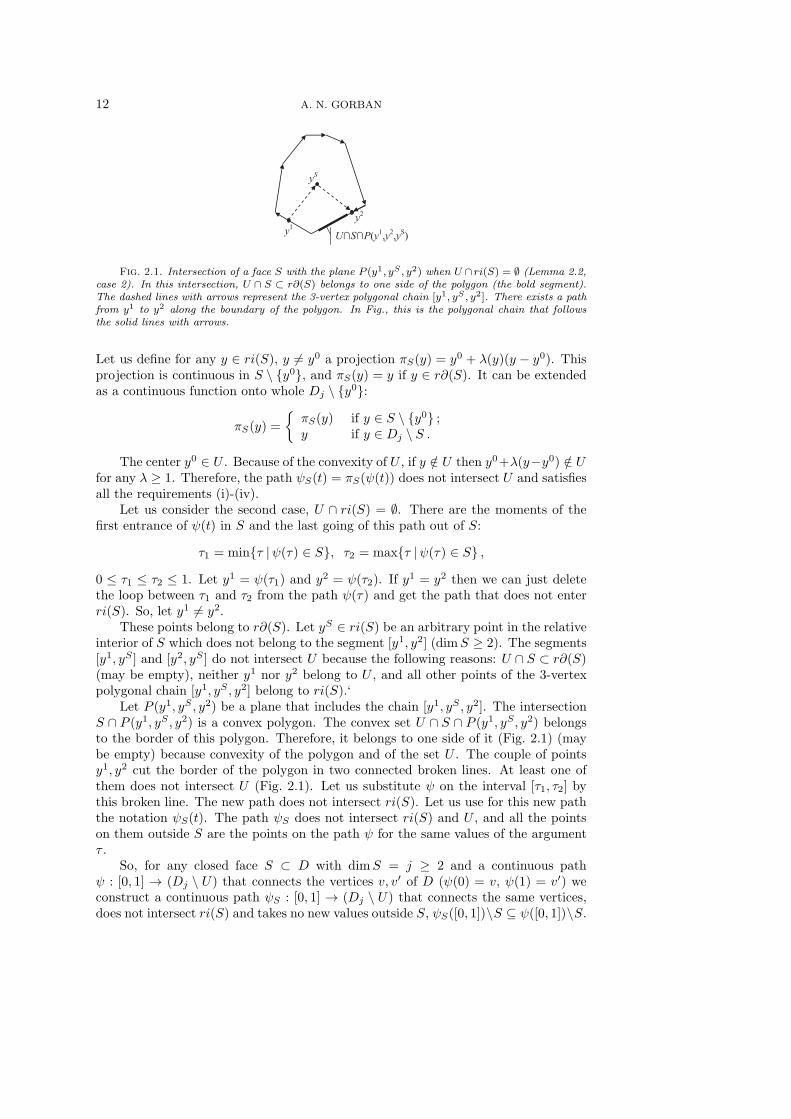
Fig. 2.1. Intersection of a face S with the plane P (y1, yS , y2) when U ∩ ri(S) = ∅ (Lemma 2.2,case 2). In this intersection, U ∩ S ⊂ r∂(S) belongs to one side of the polygon (the bold segment).The dashed lines with arrows represent the 3-vertex polygonal chain [y1, yS , y2]. There exists a pathfrom y1 to y2 along the boundary of the polygon. In Fig., this is the polygonal chain that followsthe solid lines with arrows.
Let us define for any y ∈ ri(S), y 6= y0 a projection πS(y) = y0 + λ(y)(y − y0). Thisprojection is continuous in S \ {y0}, and πS(y) = y if y ∈ r∂(S). It can be extendedas a continuous function onto whole Dj \ {y
0}:
πS(y) =
{πS(y) if y ∈ S \ {y0} ;y if y ∈ Dj \ S .
The center y0 ∈ U . Because of the convexity of U , if y /∈ U then y0+λ(y−y0) /∈ Ufor any λ ≥ 1. Therefore, the path ψS(t) = πS(ψ(t)) does not intersect U and satisfiesall the requirements (i)-(iv).
Let us consider the second case, U ∩ ri(S) = ∅. There are the moments of thefirst entrance of ψ(t) in S and the last going of this path out of S:
τ1 = min{τ |ψ(τ) ∈ S}, τ2 = max{τ |ψ(τ) ∈ S} ,
0 ≤ τ1 ≤ τ2 ≤ 1. Let y1 = ψ(τ1) and y2 = ψ(τ2). If y1 = y2 then we can just delete
the loop between τ1 and τ2 from the path ψ(τ) and get the path that does not enterri(S). So, let y1 6= y2.
These points belong to r∂(S). Let yS ∈ ri(S) be an arbitrary point in the relativeinterior of S which does not belong to the segment [y1, y2] (dimS ≥ 2). The segments[y1, yS ] and [y2, yS ] do not intersect U because the following reasons: U ∩ S ⊂ r∂(S)(may be empty), neither y1 nor y2 belong to U , and all other points of the 3-vertexpolygonal chain [y1, yS , y2] belong to ri(S).‘
Let P (y1, yS , y2) be a plane that includes the chain [y1, yS , y2]. The intersectionS ∩ P (y1, yS , y2) is a convex polygon. The convex set U ∩ S ∩ P (y1, yS, y2) belongsto the border of this polygon. Therefore, it belongs to one side of it (Fig. 2.1) (maybe empty) because convexity of the polygon and of the set U . The couple of pointsy1, y2 cut the border of the polygon in two connected broken lines. At least one ofthem does not intersect U (Fig. 2.1). Let us substitute ψ on the interval [τ1, τ2] bythis broken line. The new path does not intersect ri(S). Let us use for this new paththe notation ψS(t). The path ψS does not intersect ri(S) and U , and all the pointson them outside S are the points on the path ψ for the same values of the argumentτ .
So, for any closed face S ⊂ D with dimS = j ≥ 2 and a continuous pathψ : [0, 1] → (Dj \ U) that connects the vertices v, v′ of D (ψ(0) = v, ψ(1) = v′) weconstruct a continuous path ψS : [0, 1] → (Dj \ U) that connects the same vertices,does not intersect ri(S) and takes no new values outside S, ψS([0, 1])\S ⊆ ψ([0, 1])\S.

THERMODYNAMIC TREE 13
Let us order the faces S ⊆ D with dimS ≥ 2 in such a way that dimSi ≥ dimSj
for i < j: D = S0, S1, . . . , Sℓ. Let us start from a given path ϕ : [0, 1] → D \ U thatconnects the vertices v and v′ and let us apply sequentially the described procedure:
θ = (. . . (((ϕS0)S1
)S2) . . .)Sℓ
.
By the construction, this path θ does not intersect any relative interior ri(Sk) (k =0, 1, . . . , ℓ). Therefore, the image of θ belongs to D1, θ : [0, 1] → (D1 \ U). It can betransformed into a simple path in D1 \U by deletion of all loops (if they exist). Thissimple path (without self-intersections) is just the sequence of edges we are lookingfor.
Lemmas 2.1, 2.2 allow us to describe the connected components of the d-dimen-sional set D\U through the connected components of the one-dimensional continuumD1 \ U .
Proposition 2.3. LetW1, . . . ,Wq be all the path-connected components of D\U .Then Wi ∩ D0 6= ∅ for all i = 1, . . . , q, the continuum D1 \ U has q path-connectedcomponents and Wi ∩D1 are these components.
Proof. Due to Lemma 2.1, each path-connected component of D \ U includesat least one vertex of D. According to Lemma 2.2, if two vertices of D belong toone path-connected component of D \ U then they belong to one path-connectedcomponent of D1 \ U . The reverse statement is obvious, because D1 ⊂ D and acontinuous path in D1 is a continuous path in D.
We can study connected components of a simpler, discrete object, the graph D1.The path-connected components of D \U correspond to the connected components of
the graph D1 \ U . (This graph is produced from D1 by deletion all the vertices thatbelong to U0 and all the edges that belong to U1).
Proposition 2.4. LetW1, . . . ,Wq be all the path-connected components of D\U .
Then the graph D1 \ U has exactly q connected components and each set Wi ∩D0 is
the set of the vertices of D of one connected component of D1 \ U .Proof. Indeed, every path between vertices in D1 includes a path that connects
these vertices and is the sequence of edges. (To prove this statement we just have todelete all loops in a given path.) Therefore, the vertices v1, v2 belong to one connected
component of D1 \ U if and only if they belong to one path-connected component ofD1 \ U . The rest of the proof follows from Proposition 2.3.
We proved that the path-connected components of D \U are in one-to-one corre-
spondence with the components of the graph D1 \ U (the correspondent componentshave the same sets of vertices). In applications, we will meet the following problem.Let a point x ∈ D \ U be given. Find the path-connected component of D \ U whichincludes this point. There are two basic ways to find this component. Assume that weknow the connected components of D1 \U . First, we can examine the segments [x, v]for all vertices v of D. At least one of them does not intersect U (Lemma 2.1). Let it
be [x, v0]. We can find the connected component D1 \ U that contains v0. The pointx belongs to the correspondent path-connected component of D \ U . This approachexploits the V -description of the polyhedron D. The work necessary for this methodis proportional to the number of vertices of D.
Another method is based on projection on the faces of D. Let x ∈ ri(D). We cantake any point y0 ∈ D\U and find the unique λ1 > 1 such that x1 = y0+λ1(x−y0) ∈r∂(D). Let x1 ∈ ri(S1), where S1 is a face of D. If S1 ∩ U = ∅ then we can take
any vertex v0 ∈ S1 and find the connected component D1 \ U that contains v0. This

14 A. N. GORBAN
component gives us the answer. If S1 ∩ U 6= ∅ then we can take any y1 ∈ S1 ∩ U andfind the unique λ2 > 1 such that x2 = y1+λ2(x
1−y1) ∈ r∂(S). This x2 belongs to therelative boundary of the face S1. If x2 is not a vertex then it belongs to the relativeinterior of some face S2, dimS2 > 0 and we have to continue. At each iteration,the dimension of faces decreases. After d = dimD iterations at most we will get thevertex v we are looking for (see also Fig. 1.1) and find the connected component of
D1 \ U which gives us the answer. Here we exploit the H-description of D.
2.2. Description of the connected components of D \U by inequalities.
Let W1, . . . ,Wq be the path-connected components of D \ U .Proposition 2.5. For any set of indices I ⊂ {1, . . . , q} the set
KI = U⋃(⋃
i∈I
Wi
)
is convex.Proof. Let y1, y2 ∈ KI . We have to prove that [y1, y2] ⊂ KI . Five different
situations are possible:1. y1, y2 ∈ U ;2. y1 ∈ U, y2 ∈Wi, i ∈ I;3. y1, y2 ∈Wi, i ∈ I, [y1, y2] ∩ U = ∅;4. y1, y2 ∈Wi, i ∈ I, [y1, y2] ∩ U 6= ∅;5. y1 ∈Wi, y
2 ∈ Wj , i, j ∈ I, i 6= j.We will systematically use two simple facts: (i) the convexity of U implies that itsintersection with any segment is a segment and (ii) if x1 ∈ Wi and x
2 ∈ D \Wi thenthe segment [x1, x2] intersects U because Wi is a path-connected component of U .
In case 1, [y1, y2] ⊂ U ⊂ K because convexity U .In case 2, there exists such a point y3 ∈ (y1, y2) that [y1, y3) ⊆ U ∩ [y1, y2] ⊆
[y1, y3]. The segment (y3, y2] cannot include any point x ∈ D \Wi because it doesnot include any point from U . Therefore, in this case (y3, y2] ⊂Wi ⊂ K and y3 ∈ Kbecause it belongs either to U or to Wi.
In case 3, [y1, y2] ⊂Wi ⊂ K because Wi is a path-connected component of D \Uand [y1, y2] ∩ U = ∅.
In case 4, [y1, y2] ∩ U is a segment L with the ends x1, x2. It may be [x1, x2](y1 < x1 ≤ x2 < y2), (x1, x2] (y1 ≤ x1 < x2 < y2), [x1, x2) (y1 < x1 < x2 ≤ y2),or (x1, x2) (y1 ≤ x1 < x2 ≤ y2). This segment cuts [y1, y2] in three segments:[y1, y2] = L1∪L∪L2, L1 includes y1 and L2 includes y2. Therefore, L1 ⊂Wi, L ⊂ Uand L2 ⊂ Wi because Wi is a path-connected component of D \ U and U is convex.So, [y1, y2] ⊂ K.
In case 5, [y1, y2]∩U is also a segment L with the ends x1, x2. It may be [x1, x2](y1 < x1 ≤ x2 < y2), (x1, x2] (y1 ≤ x1 < x2 < y2), [x1, x2) (y1 < x1 < x2 ≤ y2),or (x1, x2) (y1 ≤ x1 < x2 ≤ y2). This segment cuts [y1, y2] in three segments:[y1, y2] = L1∪L∪L2, L1 includes y1 and L2 includes y2. Therefore, L1 ⊂Wi, L ⊂ Uand L2 ⊂Wj because Wi,j are path-connected components of D \U and U is convex.So, [y1, y2] ⊂ K.
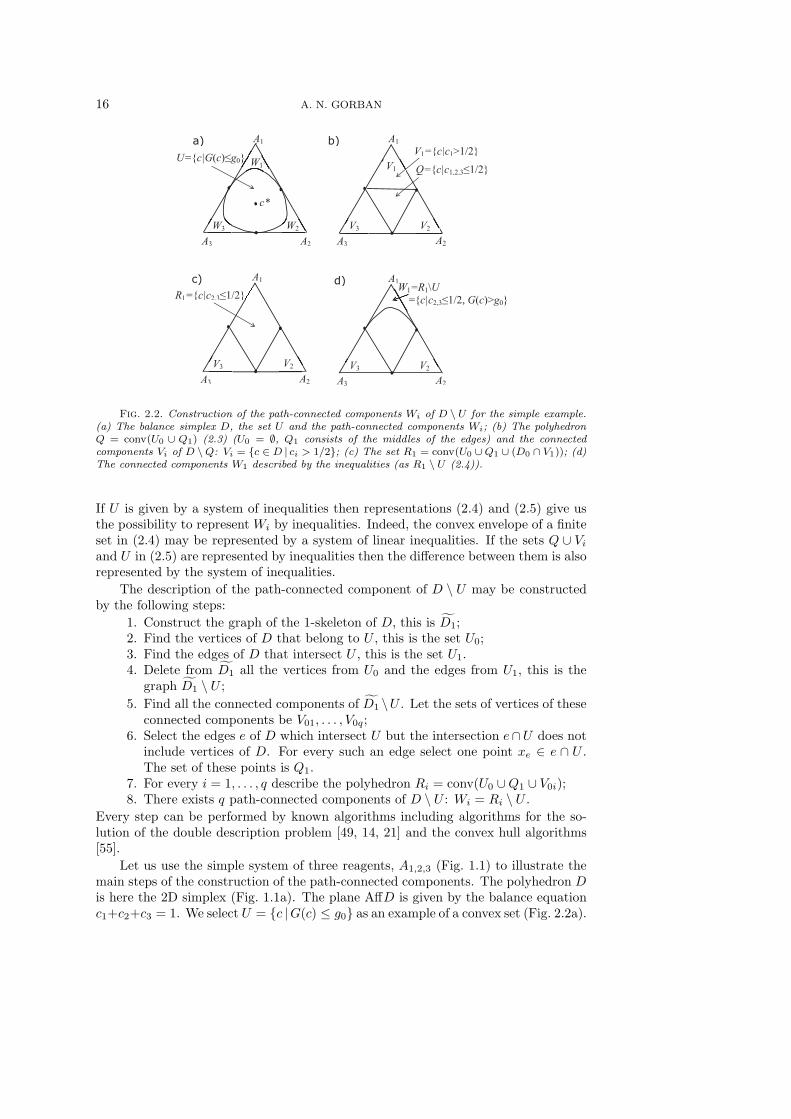
Typically, the set U is represented by a set of inequalities, for example, G(x) ≤ g.It may be useful to represent the path-connected components of D\U by inequalities.For this purpose, let us first construct a convex polyhedron Q ⊂ U with the samenumber of path-connected components in D \Q, V1, . . . , Vq and with inclusons Wi ⊂Vi. We will construct Q as a convex hull of a finite set. Let us select the edges e of D

THERMODYNAMIC TREE 15
which intersect U but the intersection e∩U does not include vertices of D. For everysuch edge we select one point xe ∈ e∩U . The set of these points is Q1. By definition,
Q = conv(U0 ∪Q1) . (2.3)
Q is convex, hence, we can apply all the previous results about the components ofD \ U to the components of D \Q.
Lemma 2.6. The set U0 ∪Q1 is the set of vertices of Q.Proof. A point x ∈ U0∪Q1 is not a vertex of Q = conv(U0∪Q1) if and only if it is a
convex combination of other points from this set: there exist such x1, . . . , xk ∈ U0∪Q1
and λ1, . . . , λk > 0 that xi 6= x for all i = 1, . . . , k and
k∑
i=1
λi = 1 ,k∑
i=1
λixi = x .
If x ∈ U0 then this is impossible because x is a vertex of D and U0 ∪ Q1 ⊂ D. Ifx ∈ Q1 then it belongs to the relative interior of an edge of D and, hence, may be aconvex combination of points D from this edge only. By construction, U0 ∪ Q1 mayinclude only one internal point from an edge and in this case does not include a vertexfrom this edge. Therefore, all the points from Q1 are vertices of Q.
Lemma 2.7. The set D \Q has q path-connected components V1, . . . , Vq that maybe enumerated in such a way that Wi ⊂ Vi and Wi = Vi \ U .
Proof. To prove this statement about the path-connected components, let usmention that Q and U include the same vertices of D, the set U0, and cut the sameedges of D. Graphs D1 \Q and D1 \ U coincide. Q ⊂ U because of the convexity ofU and definition of Q. To finalize the proof, we can apply Proposition 2.4.
Proposition 2.8. Let I be any set of indices from {1, . . . , q}.
Q⋃(⋃
i∈I
Vi
)= conv
(U0
⋃Q1
⋃(⋃
i∈I
(D0
⋂Vi
)))(2.4)
Proof. On the left hand side of (2.4) we see the union of Q with the connectedcomponents Vi (i ∈ I). On the right hand side there is a convex envelope of a finiteset. This finite set consists of the vertices of Q, (U0 ∪Q1) and the vertices of D thatbelong to Vi (i ∈ I). Let us denote by RI the right hand side of (2.4) and by LI theleft hand side of (2.4).
LI is convex due to Proposition 2.5 applied to Q and Vi. The inclusion RI ⊆ LI isobvious because LI is convex and RI is defined as a convex hull of a subset of LI . Toprove the inverse inclusion, let us consider the path-connected components of D \RI .Sets Vj (j /∈ I) are the path-connected components of D \ RI because they are thepath-connected components of D \Q, Q ⊂ RI and RI ∩ Vj = ∅ for j /∈ I. There existno other path-connected components of Q ⊂ RI because all the vertices of Vi (i ∈ I)belong to RI by construction, hence, D0 \ RI ⊂ ∪j /∈IVj . Due to Lemma 2.1 everypath-connected component of D ⊂ RI includes at least one vertex of D. Therefore,Vj (j /∈ I) are all the path-connected components of D \ RI and D \ RI = ∪j /∈IVj .Finally, RI = D \ ∪j /∈IVj = Q ∪ (∪i∈IVi) = LI .
According to Lemma 2.6, each path-connected component Wi ⊂ D \ U can berepresented in the form Wi = Vi \ U , where Vi is a path-connected component ofD \Q. By construction, Q ⊂ U , hence
Wi = (Q ∪ Vi) \ U . (2.5)
16 A. N. GORBAN
A1
A2 A3
c*
U={c|G(c)≤g0}
a)
W1`
W3 W2
c) A1
A2 A3
V3 V2
R1={c|c2,3≤1/2}
b) A1
A2 A3
V3 V2
Q={c|c1,2,3≤1/2} V1
d) A1
A2 A3
V3 V2
A1W1=R1\U
={c|c2,3≤1/2, G(c)>g0}
V1={c|c1>1/2}
Fig. 2.2. Construction of the path-connected components Wi of D \ U for the simple example.(a) The balance simplex D, the set U and the path-connected components Wi; (b) The polyhedronQ = conv(U0 ∪ Q1) (2.3) (U0 = ∅, Q1 consists of the middles of the edges) and the connectedcomponents Vi of D \Q: Vi = {c ∈ D | ci > 1/2}; (c) The set R1 = conv(U0 ∪Q1 ∪ (D0 ∩ V1)); (d)The connected components W1 described by the inequalities (as R1 \ U (2.4)).
If U is given by a system of inequalities then representations (2.4) and (2.5) give usthe possibility to represent Wi by inequalities. Indeed, the convex envelope of a finiteset in (2.4) may be represented by a system of linear inequalities. If the sets Q ∪ Viand U in (2.5) are represented by inequalities then the difference between them is alsorepresented by the system of inequalities.
The description of the path-connected component of D \ U may be constructedby the following steps:
1. Construct the graph of the 1-skeleton of D, this is D1;2. Find the vertices of D that belong to U , this is the set U0;3. Find the edges of D that intersect U , this is the set U1.4. Delete from D1 all the vertices from U0 and the edges from U1, this is the
graph D1 \ U ;
5. Find all the connected components of D1 \U . Let the sets of vertices of theseconnected components be V01, . . . , V0q;
6. Select the edges e of D which intersect U but the intersection e∩U does notinclude vertices of D. For every such an edge select one point xe ∈ e ∩ U .The set of these points is Q1.
7. For every i = 1, . . . , q describe the polyhedron Ri = conv(U0 ∪Q1 ∪ V0i);8. There exists q path-connected components of D \ U : Wi = Ri \ U .
Every step can be performed by known algorithms including algorithms for the so-lution of the double description problem [49, 14, 21] and the convex hull algorithms[55].
Let us use the simple system of three reagents, A1,2,3 (Fig. 1.1) to illustrate themain steps of the construction of the path-connected components. The polyhedron Dis here the 2D simplex (Fig. 1.1a). The plane AffD is given by the balance equationc1+c2+c3 = 1. We select U = {c |G(c) ≤ g0} as an example of a convex set (Fig. 2.2a).
THERMODYNAMIC TREE 17
It includes no vertices of D, hence, U0 = ∅. U intersects each edge of D in the middlepoint, hence, U1 includes all the edges of D. The graph D1 \ U consists of threeisolated vertices. Its connected components are these isolated vertices. Q1 consists ofthree points, the middles of the edges (1/2, 1/2, 0), (1/2, 0, 1/2) and (0, 1/2, 1/2) (inthis example, the choice of these points is unambiguous, Fig. 2.2a).
The polyhedron Q is a convex hull of these three points, that is the triangle givenin Aff(D) by the system of three inequalities c1,2,3 ≤ 1/2 (Fig. 2.2b). The connectedcomponents of D \Q are the triangles Vi given in D by the inequalities ci > 1/2. Inthe whole R3, these sets are given by the systems of an equation and inequalities:
Vi = {c | c1,2,3 ≥ 0, c1 + c2 + c3 = 1, ci > 1/2} .
The polyhedron Ri is the convex hull of four points, the middles of the edges andthe ith vertex (Fig. 2.2c). In D, Ri is given by two linear inequalities, cj ≤ 1/2, j 6= i.In the whole R3, these inequalities should be supplemented by the equation andinequalities that describe D:
Ri = {c | c1,2,3 ≥ 0, c1 + c2 + c3 = 1, cj ≤ 1/2 (j 6= i)} .
The path-connected components of D \U , Wi are described as Ri \U Fig. 2.2d):in D we get Wi = {c | cj ≤ 1/2 (j 6= i), G(c) > g0}. In the whole R3,
Wi = {c | c1,2,3 ≥ 0, c1 + c2 + c3 = 1, cj ≤ 1/2 (j 6= i), G(c) > g0} .
Vi are convex sets in this simple example, therefore, it is possible to simplifyslightly the description of the components Wi and to represent them as Vi \ U :
Wi = {c | c1,2,3 ≥ 0, c1 + c2 + c3 = 1, ci > 1/2, G(c) > g0}
(or Wi = {c | ci > 1/2, G(c) > g0} in D).In the general case (more components and balance conditions), the connected
components Vi may be non-convex, hence, description of these sets by the systemsof linear equations and inequalities may be impossible. Nevertheless, there existsanother version of the description of Wi where a smaller polyhedron is used insteadof Ri
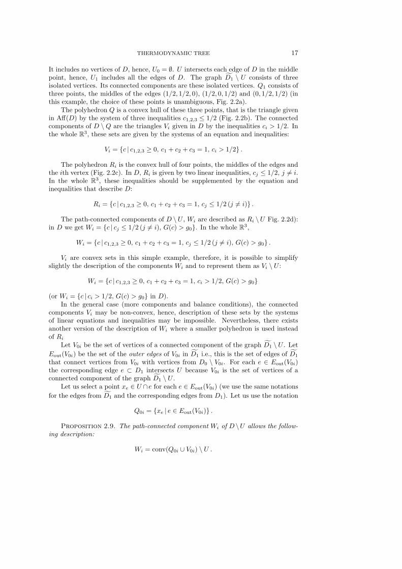
Let V0i be the set of vertices of a connected component of the graph D1 \U . Let
Eout(V0i) be the set of the outer edges of V0i in D1 i.e., this is the set of edges of D1
that connect vertices from V0i with vertices from D0 \ V0i. For each e ∈ Eout(V0i)the corresponding edge e ⊂ D1 intersects U because V0i is the set of vertices of aconnected component of the graph D1 \ U .
Let us select a point xe ∈ U ∩ e for each e ∈ Eout(V0i) (we use the same notations
for the edges from D1 and the corresponding edges from D1). Let us use the notation
Q0i = {xe | e ∈ Eout(V0i)} .
Proposition 2.9. The path-connected component Wi of D \U allows the follow-ing description:
Wi = conv(Q0i ∪ V0i) \ U .
18 A. N. GORBAN
Proof. The set Q0i ⊂ U and V0i is the set of vertices of a connected componentof the graph D1 \Q0i by construction because Q0i cuts all the outer edges of V0i inD1. The rest of the proof follows the proofs of Lemma 2.7 and Proposition 2.8.
This proposition allows us to describe Wi by the system of inequalities. Forthis purpose, we have to use a convex hull algorithm and describe the convex hullconv(Q0i ∪ V0i) by the system of linear inequalities and then add the inequality thatdescribes the set \U .
In the simple system (Fig. 2.2), the connected components of the graph D1 \ Uare the isolated vertices. The set Q0i for the vertex Ai consists of two middles of itsincident edges. In Fig. 2.2b, the set conv(Q0i ∪ V0i) for V0i = {A1} is the triangle V1.
3. Thermodynamic tree.
3.1. Problem statement. Let a real continuous function G be given in theconvex bounded polyhedron D ⊂ Rn. We assume that G is strictly convex in D, i.e.the set (the epigraph of G)
epi(G) = {(x, g) |x ∈ D, g ≥ G(x)} ⊂ D × (−∞,∞)
is convex and for any segment [x, y] ⊂ D (x 6= y) G is not constant on [x, y]. Astrictly convex function on a bounded convex set has a unique minimizer. Let x∗ be theminimizer of G inD and let g∗ = G(x∗) be the corresponding minimal value. The levelset Sg = {x ∈ D |G(x) = g} is closed and the sublevel set Ug = {x ∈ D |G(x) < g}is open in D. The sets Sg and D \ Ug are compact and Sg ⊂ D \ Ug.
Let x, y ∈ D. According to Corollary 3.4 proven in the next subsection, anadmissible path from x to y in D exists if and only if π(y) belongs to the orderedsegment [π(x∗), π(x)]. Therefore, to describe constructively the relation x % y in Dwe have to solve the following problems:
1. How to construct the thermodynamic tree T ?2. How to find an image π(x) of a state x ∈ D on the thermodynamic tree T ?3. How to describe by inequalities a preimage of an ordered segment of the
thermodynamic tree, π−1([w, z]) ⊂ D (w, z ∈ T , z % w)?
3.2. Coordinates on the thermodynamic tree . We get the following lemmadirectly from Definition 1.1. Let x, y ∈ D.
Lemma 3.1. x ∼ y if and only if G(x) = G(y) and x and y belong to the samepath-connected component of Sg with g = G(x).
The path-connected components of D \ Ug can be enumerated by the connected
components of the graph D1 \Ug. The following lemma allows us to apply this resultto the path-connected components of Sg.
Lemma 3.2. Let g > g∗, W1, . . . ,Wq be the path-connected components of D \Ug
and let σ1, . . . , σp be the path-connected components of Sg. Then q = p and σi maybe enumerated in such a way that σi is the border of Wi in D.
Proof. G is continuous in D, hence, if G(x) > g then there exists a vicinity of xin D where G(x) > g. Therefore G(y) = g for every boundary point y of D \Ug in Dand Sg is the boundary of D \ Ug in D.
Let us define a projection θg : D \ Ug → Sg by the conditions: θg(x) ∈ [x, x∗]and G(θg(x)) = g. By definition, the inequality G(x) ≥ g holds in D \ Ug. Thefunction fx(λ) = G((1 − λ)x∗ + λx) is strictly increasing, continuous and convexfunction of λ ∈ [0, 1], fx(0) = g∗ < g, fx(1) = G(x) ≥ g. The function fx(λ)depends continuously on x ∈ D \ Ug in the uniform metrics. Therefore, the solution
THERMODYNAMIC TREE 19
λx to the equation fx(λ) = g on [0, 1] exists (the intermediate value theorem), isunique, and continuously depends on x ∈ D \ Ug. The projection θg is defined asθg(x) = (1 − λx)x
∗ + λxx.The fixed points of the projection θg are elements of Sg. The image of each
path-connected component Wi is a path-connected set. The preimage of every path-connected component σi is also a path-connected set. Indeed, let θg(x) ∈ σi andθg(y) ∈ σi. There exists a continuous path from x to y in D\Ug. It may be composedfrom three paths: (i) from x to θg(x) along the line segment [x, θg(x)] ⊂ [x, x∗]then a continuous path in σi between θg(x) and θg(y) (it exists because σi is a path-connected component of Sg and it belongs to D\Ug because Sg ⊂ D\Ug) and, finally,from θg(y) to y along the line segment [θg(y), y] ⊂ [x∗, y]. Therefore, the image ofa path-connected component Wi is a path-connected components of Sg that may beenumerated by the same index i, σi. This σi is the border of Wi in D.
The equivalence class of x ∈ D is defined as [x] = {y ∈ D | y ∼ x}. Let W (x) bea path-connected component of D \Ug (g = G(x)) for which θg(W (x)) = [x]. Due toLemma 3.2, such a component exists and
W (x) = {y ∈ D | y % x} . (3.1)
Let us define a one-dimensional continuum Y that consists of the pairs (g,M),
where g∗ ≤ g ≤ gmax and M is a set of vertices of a connected component of D1 \Ug.For each (g,M) the fundamental system of neighborhoods consists of the sets Vρ(ρ > 0):
Vρ = {(g′,M ′) | (g′,M ′) ∈ Y, |g − g′| < ρ, M ′ ⊆M} . (3.2)
Let us define the partial order on Y:
(g,M) % (g′,M ′) if g ≥ g′ and M ⊆M ′ .
Let us introduce the mapping ω : D → Y:
ω(x) = (G(x),W (x) ∩D0) .
Theorem 3.3. There exists a homeomorphism between Y and T that preservesthe partial order and makes the following diagram commutative:
Dπ
//
ω
��
T??
��⑦⑦⑦⑦⑦⑦⑦⑦
Y
Proof. According to Lemmas 3.2, 3.1 and Proposition 2.4, ω maps the equivalentpoints x to the same pair (g,M) and the non-equivalent points to different pairs(g,M). For any x, y ∈ D, x % y if and only if ω(x) % ω(y).
The fundamental system of neighborhoods in Y may be defined using this partialorder. Let us say that (g,M) is compatible to (g′,M ′) if (g′,M ′) % (g,M) or (g,M) %(g′,M ′)}. Then for ρ > 0
Vρ = {(g′,M ′) ∈ Y | |γ − γ′| < ρ and (g′,M ′) is compatible to (g,M)} .
For sufficiently small ρ this definition coincides with (3.2).
20 A. N. GORBAN
So, by the definition of T as a quotient space D/ ∼, Y has the same partialorder and topology as T . The isomorphism between Y and T establishes one-to-one correspondence between the π-image of the equivalence class [x], π([x]), and theω-image of the same class, ω([x]).
Y can be considered as a coordinate system on T . Each point is presented as apair (g,M) where g∗ ≤ g ≤ gmax and M is a set of vertices of a connected component
of D1 \ Ug. The map ω is the coordinate representation of the canonical projectionπ : D → T . Now, let us use this coordinate system and the proof of Theorem 3.3 toobtain the following corollary.
Corollary 3.4. An admissible path from x to y in D exists if and only if
π(y) ∈ [π(x∗), π(x)] .
Proof. Let there exist an admissible path from x to y in D, ϕ : [0, 1] → D.Then π(x) % π(y) in T . Let π(x) = (G(x),M) in coordinates Y. For any v ∈ M ,π(y) ∈ [π(x∗), π(v)] and π(x) ∈ [π(x∗), π(v)].
Assume now that π(y) ∈ [π(x∗), π(x)] and π(x) = (G(x),M). Then the admissiblepath from x to y in D can be constructed as follows. Let v ∈ M be a vertex of D.G(v) ≥ G(x) for each v ∈ M . The straight line segment [x∗, v] includes a point x1with G(x1) = G(x) and y1 with G(y1) = G(y). Coordinates of π(x1) and π(x) in Ycoincide as well as coordinates of π(y1) and π(y). Therefore, x ∼ x1 and y ∼ y1. Theadmissible path from x to y in D can be constructed as a sequence of three paths:first, a continuous path from x to x1 inside the path-connected component of SG(x)
(Lemma 3.1), then from x1 to y1 along a straight line and after that a continuouspath from y1 to y inside the path-connected component of SG(y).
To describe the space T in coordinate representation Y, it is necessary to find theconnected components of the graph D1 \ Ug for each g. First of all, this function,
g 7→ the set of connected components of D1 \ Ug ,
is piecewise constant. Secondly, we do not need to solve at each point the computa-tionally heavy problem of the construction of the connected components of the graphD1 \Ug “from scratch”. The problem of the parametric analysis of these componentsas functions of g appears to be much cheaper. Let us present a solution of this prob-lem. At the same time, this is a method for the construction of the thermodynamictree in coordinates (g,M).
The coordinate system Y allows us to describe the tree structure of the continuumT . This structure includes a root, (g∗, D0), edges, branching points and leaves.
LetM be a connected component of D1\Ug for some g, g∗ < g < gmax. IfM $ D0
then the set of all points (g,M) ∈ T has for a given M the form (aM , aM ] × M ,aM < aM . We call this set an edge of T .
IfM includes all the vertices of D (M = D0) then the set of all points (g,M) ∈ Thas the form [g∗, aD0
]×D0. This may be either an edge (if aD0> g∗) or just a root,
{(g∗, D0)}, (this is possible in 1D systems).Let us define the numbers aM = inf{g | (g,M) ∈ T }. Let us introduce the set of
outer edges of M in D1, Eout(M). This is the set of edges of D1 that connect verticesfrom M with vertices from D0 \M . We keep the same notation, Eout(M), for the setof the corresponding edges of D.
aM = maxe∈Eout(M)
min{G(x) |x ∈ e} . (3.3)
THERMODYNAMIC TREE 21
This number, aM , is the “cutting value” of G forM . It cutsM from the other vertices
of D1 in the following sense: if we delete from D1 all the edges e with the label values< aM then M will remain attached to some vertices from D0 \M . If we delete theedges with the label values ≤ aM then M becomes disconnected from D0 \M . There
is the only connected component of D1 \ UaM
that includes M , M ′ % M . The pair(aM ,M
′) ∈ T is a branching point of T . The edge (aM , aM ]×M connects two vertices,the upper vertex (aM ,M) and the lower vertex, (aM ,M
′).If M consists of one vertex, M = {v}, then the point (G(v), {v}) is a leaf of T .
3.3. Construction of the thermodynamic tree. To construct the tree ofG inD we need the graph D1 of the 1-skeleton of the polyhedronD. Elements of D1 shouldbe labeled by the values of G. Each vertex v is labeled by the value γv = G(v) andeach edge e = [v, w] is labeled by the minimal value of G on the segment [v, w] ⊂ D,ge = min[v,w]G(x). We need also the minimal value g∗ = minD{G(x)} because theroot of the tree is (g∗, D0).
The strictly convex function G achieves its local maxima in D only in vertices.The vertex v is a (local) maximizer of g if ge < γv for each edge e that includes v.The leaves of the thermodynamic tree are pairs (γv, {v}) for the vertices that are thelocal maximizers of G.
As a preliminary step of the construction, we arrange and enumerate the labelsof the elements of D1, the vertices and edges, in descending order. Let there exist ldifferent label values: gmax = a1 > a2 > . . . > al. Each ak is a value γv = G(v) ata vertex v ∈ D0 or the minimum of G on an edge e ⊂ D1 (or both). Let Ai be theset of vertices v ∈ D0 with γv = ai and let Ei be the set of edges of D1 with ge = ai(i = 1, . . . , l).
Let us construct the connected components of the graph D1 \ Ug starting froma1 = gmax. The function G is strictly convex, hence, a1 = γv for a set of verticesA1 ⊂ D0 but it is impossible that a1 = ge for an edge e, hence, E1 = ∅.
The set of connected components of D1 \Ug is the same for all g ∈ (ai+1, ai]. For
an interval (a2, a1] the connected components of D1 \Ug are the one-element sets {v}for v ∈ A1.
For g ∈ [g∗, al] the graph D1 \ Ug includes all the vertices and edges of D1 and,hence, it is connected for this segment. Let us take, formally, al+1 = g∗.
Let Li = {M i1, . . . ,M
iki} be the set of the connected components of D1 \ Ug for
g ∈ (ai, ai−1] (i = 1, . . . , l). Each connected component is represented by the set ofits vertices M i
j . Let us describe the recursive procedure for construction of Li:1. Let us take formally L0 = ∅.2. Assume that Li−1 is given and i ≤ l. Let us find the set Li of connected
components of D1 \ Ug for g = ai (and, therefore, for g ∈ (ai+1, ai]).• Add the one-element sets {v} for all v ∈ Ai to the set
Li−1 = {M i−11 , . . . ,M i−1
ki−1} .
Denote this auxiliary set of sets as Li,0 = {M1, . . . ,Mq}, where q =ki−1 + |Ai|.
• Enumerate the edges from Ei in an arbitrary order: e1, . . . , e|Ei|. For
each k = 0, . . . , |Ei|, create recursively an auxiliary set of sets Li,k by the
union of some of elements of Lk−1: Let Li,k−1 be given and ek connects
the vertices v and v′. If v and v′ belong to the same element of Li,k−1
22 A. N. GORBAN
then Li,k = Li,k−1. If v and v′ belong to the different elements of Li,k−1,
M and M ′, then Li,k is produced from Li,k−1 by the union of M andM ′:
Li,k = (Li,k−1 \ {M} \ {M ′}) ∪ {M ∪M ′}
(we delete two elements, M andM ′, from Li,k−1 and add a new elementM ∪M ′).
The set Li of connected components of D1 \ Ug for g = ai is Li = Li,|Ei|.
Generically, all the labels of the graph D1 vertices and edges are different and the setsEi and Ai include not more than one element. Moreover, for each i either Ei or Ai
is generically empty and the description of the recursive procedure may be simplifiedfor the generic case:
1. Let us take formally L0 = ∅.2. Assume that Li−1 is given and i ≤ l.
• If ai is a label of a vertex v, ai = γv, then add the one-element set {v}to the set Li−1: Li = Li−1 ∪ {{v}}.
• Let ai be a label of an edge e = [v, v′]. If v and v′ belong to the sameelement of Li−1 then Li = Li−1. If v and v′ belong to the differentelements of Li−1, M and M ′, then Li is produced from Li−1 by theunion of M and M ′ (delete elements M and M ′ and add an elementM ∪M ′).
The described procedure gives us the sets of connected components of D1 \ Ug
for all g and, therefore, we get the tree T . The descent from the higher values of Gallows us to avoid the solution of the computationally more expensive problem of thecalculation of the connected components of a graph at any level of G.
3.4. The problem of attainable sets. In this section, we demonstrate how tosolve the problem of attainable sets. For given x ∈ D (an initial state) we describethe attainable set
Att(x) = {y ∈ D |x % y}
by a system of inequalities. Let the tree T of G in D be given and let all the pairs(g,M) ∈ T be described. We also use the notation Att(z) for sets attainable in Tfrom z ∈ T .
First of all, let us describe the preimage of a point (g,M) ∈ T in D. It can bedescribed by the equation G(x) = g and a set of linear inequalities. For each edge e weselect a minimizer of G on e, xe = argmin{G(x) |x ∈ e} (we use the same notations
for the elements of the graph D1 and of the continuum D1). Let
QM = {xe | e ∈ Eout(M)} .
In particular, aM = max{G(x) |x ∈ QM}.The following Proposition is a direct consequence of Proposition 2.9.Proposition 3.5. The preimage of (g,M) in D is a set
π−1(g,M) = {x ∈ conv(QM ∪M) |G(x) = g} . (3.4)
The sets M and QM in (3.4) do not depend on the specific value of g. It issufficient that the point (g,M) ∈ T exists.

THERMODYNAMIC TREE 23
D
[ES]
[S]
bE [E]=0
bS
bS
E, P
ES, P
E, S
ES, S a) bS>bE
[ES]
[S]
[E]=0 bS=bE
bS
D
E, P
ES
E, S
b) bS=bE
D1 D1
bS
[ES]
[S]
[E]=0 bE
bS
D
E, P
E, ES
E, S
c) bS<bE
D1
Fig. 4.1. The balance polygon D on the plane with coordinates [S] and [ES] for the four–component enzyme–substrate system S, E, ES P with two balance conditions, bS = [S]+[ES]+[P ] =const and bE = [E] + [ES] = const.
Let us consider the second projection of T , i.e., the set of all connected compo-nents of the graph D1 \ Ug for all g. For a connected component M , the lower chainof connected components is a sequence M = M1 $ M2 $ . . . $ Mk. (“Lower” heremeans the descent in the natural order in T , %.) For a given initial element M =M1
the maximal lower chain of M is the lower chain of M that cannot be extendedby adding new elements. By construction of connected components, the maximallower chain of M is unique for each initial element M . In the maximal lower chainaMi
= aMi+1.
For each set of values H ⊂ (aM , aM ] the preimage of the set H ×M ⊂ T is givenby (3.4) as
π−1(H ×M) = {x ∈ conv(QM ∪M) |G(x) ∈ H} . (3.5)
We describe the set Att(x) for x ∈ D by the following procedures: (i) find theprojection π(x) of x onto T , (ii) find the attainable set in T from π(x), Att(π(x)),and (iii) find the preimage of this set in D:
Att(x) = π−1(Att(π(x))) . (3.6)
The attainable set Att(g,M) in T from (g,M) ∈ T is constructed as a union ofedges and its parts. Let M = M1 $ M2 $ . . . $ Mk = D0 be the maximal lowerchain of M . Then
Att(g,M) =(a1, g]×M1 ∪ (a2, a1]×M2 ∪ . . .
∪ (ak−1, ak−2]×Mk−1 ∪ [ak, ak−1]×Mk ,(3.7)
where ai = aMi.
To find the preimage of Att(g,M) in D we have to apply formula (3.5) to eachterm of (3.7). In Sec. 1.3 we demonstrated how to find π(x). Therefore, each step ofthe solution of the problem of attainable set (3.6) is presented.
4. Chemical thermodynamics: examples.
4.1. Skeletons of the balance polyhedra. In chemical thermodynamics andkinetics, the variable Ni is the amount of the ith component in the system. Thebalance polyhedronD is described by the positivity conditions Ni ≥ 0 and the balanceconditions (1.1) bi(N) = const (i = 1, . . . ,m). Under the isochoric (the constantvolume) conditions, the concentrations ci also satisfy the balance conditions and wecan construct the balance polyhedron for concentrations. Sometimes, the balance
24 A. N. GORBAN
bO
bH
bH>2bO
bH=2bO
2bO>bH>bO
bH=bO
bH<bO
H2, OH
H2, O
H2, H2O
H, H2O
H, O
H, OH
H2, O2
H, O2
H2, OH
H2, O
H2O
H, O
H, OH
H2, O2
H, O2
H2, OH
H2, O
O2, H2O
O, H2O
H, O
H, OH
H2, O2
H, O2
H2O, OH
OH
H2, O
O2, H2O
O, H2O
H, O
H2, O2
H, O2
O, OH
O2, OH
O2, H
O2, H2O
O, H2O
H, O
O2, H2
O, H2
a)
b) c)
d)
e)
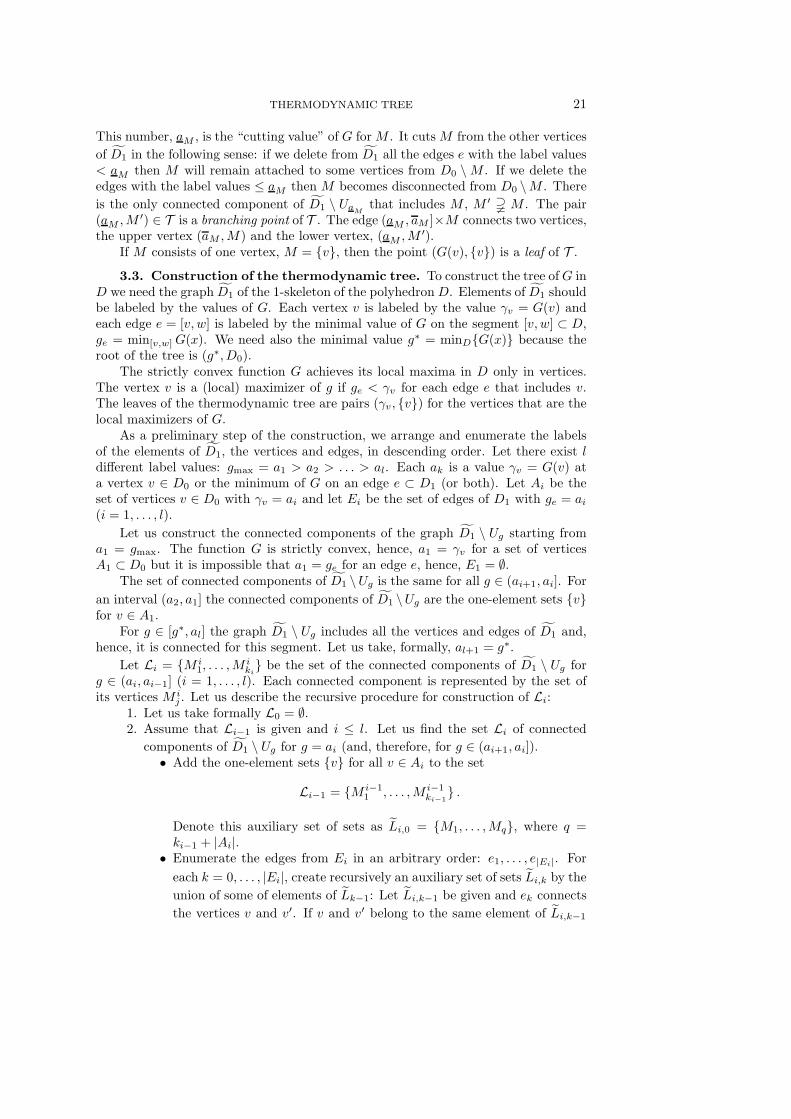
Fig. 4.2. The graph D1(b) of the one-skeleton of the balance polyhedron for the six-componentsystem, H2, O2, H, O, H2O, OH, as a piece-wise constant function of b = (bH, bO). For each vertexthe components are indicated which have non-zero concentrations at this vertex.
polyhedron is called the reaction simplex with some abuse of language because it isnot obligatory a simplex when the number m of the independent balance conditionsis greater than one.
The graph D1 depends on the values of the balance functionals bi = bi(N) =∑nj=1 a
jiNj . For the positive vectors N , the vectors b with coordinates bi = bi(N)
form a convex polyhedral cone in Rm. Let us denote this cone by Λ. D1(b) is a piece-wise constant function on Λ. Sets with various constant values of this function arecones. They form a partition of Λ. Analysis of this partition and the correspondingvalues of D1 can be done by the tools of linear programming [26]. Let us representseveral examples.
In the first example, the reaction system consists of four components: the sub-strate S, the enzyme E, the enzyme-substrate complex ES and the product P . weconsider the system under constant volume. We denote the concentrations by [S],[E], [ES] and [P ]. There are two balance conditions: bS = [S] + [ES] + [P ] = constand bE = [E] + [ES] = const.
For bS > bE the polyhedron (here the polygon) D is a trapezium (Fig. 4.1a).Each vertex corresponds to two components that have non-zero concentrations in thisvertex. For bS > bE there are four such pairs, (ES, P ), (ES, S), (E,P ) and (E, S).For two pairs there are no vertices: for (S, P ) the value bE is zero and for (ES,E) itshould be bS < bE . When bS = bE , two vertices, (ES, P ) and (ES, S), transform intoone vertex with one non-zero component, ES, an the polygon D becomes a triangle(Fig. 4.1b). When bS < bE then D is also a triangle and a vertex ES transforms inthis case into (ES,E) (Fig. 4.1c).
For the second example, we select a system with six components and two balance

THERMODYNAMIC TREE 25
H2, OH
H2, O
H2, H2O
H, H2O
H, O
H, OH
H2, O2
H, O2
H2, OH
H2, O
H2O
H, O
H, OH
H2, O2
H, O2
H2, OH
H2, O
O2, H2O
O, H2O
H, O
H, OH
H2, O2
H, O2
H2O, OH
a)
H2, OH
H2, O
O2, H2O
O, H2O
H, O
H, OH
H2, O2
H, O2
H2O, OH OH
H2, O
O2, H2O
O, H2O
H, O
H2, O2
H, O2
O, OH
O2, OH
O2, H
O2, H2O
O, H2O
H, O
O2, H2
O, H2
b)
Fig. 4.3. Transformations of the graph D1(b) with changes of the relation between bH and bO:(a) transition from the regular case bH > 2bO to the regular case 2bO > bH > bO through the singularcase bH = 2bO, (b) transition from the regular case 2bO > bH > bO to the regular case bH < bOthrough the singular case bH = bO.
conditions: H2, O2, H, O, H2O, OH;
bH = 2NH2+NH + 2NH2O +NOH ,
bO = 2NO2+NO +NH2O +NOH .
The cone Λ is a positive quadrant on the plane with the coordinates bH, bO. Thegraph D1(b) is constant in the following cones in Λ (bH, bO > 0): (a) bH > 2bO, (b)bH = 2bO, (c) 2bO > bH > bO, (d) bH = bO and (e) bH < bO (Fig. 4.2).
The cases (a) bH > 2bO, (c) 2bO > bH > bO, and (e) bH < bO (Fig. 4.2) areregular: there are two independent balance conditions and for each vertex there areexactly two components with non-zero concentration. In case (a) (bH > 2bO), ifbH → 2bO then two regular vertices, H2, H2O and H, H2O, join in one vertex (case(b)) with only one non-zero concentration, H2O (Fig. 4.3a). This vertex explodes inthree vertices O, H2O; O2, H2O and H2O, OH, when bH becomes smaller than 2bO(case (c), 2bO > bH > bO) (Fig. 4.3a). Analogously, in the transition from the regularcase (c) to the regular case (e) through the singular case (d) (bH = bO) three verticesjoin in one, 0H that explodes in two (Fig. 4.3b).
For the modeling of hydrogen combustion, the eight-component model is usedusually: H2, O2, H, O, H2O, OH, H2O2, HO2. In Fig. 4.4 the graph D1 is presentedfor one particular relations between bH and 2bO, bH = 2bO. This is the so-called“stoichiometric mixture” where proportion between bH and 2bO is the same as in the“product”, H2O.
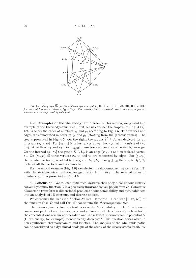
26 A. N. GORBAN
H2, OH
H2, O2
H, O2
H, OH
H, O
H2, O H2O
H2, HO2 H2, H2O2
H, HO2 H, H2O2
Fig. 4.4. The graph D1 for the eight-component system, H2, O2, H, O, H2O, OH, H2O2, HO2
for the stoichiometric mixture, bH = 2bO. The vertices that correspond also to the six-componentmixture are distinguished by bold font.
4.2. Examples of the thermodynamic tree. In this section, we present twoexample of the thermodynamic tree. First, let us consider the trapezium (Fig. 4.1a).Let us select the order of numbers γv and ge according to Fig. 4.5. The vertices andedges are enumerated in order of γv and ge (starting from the greatest values). The
tree is presented in Fig. 4.5. On the right, the graphs D1 \ Ug are depicted for allintervals (ai−1, ai]. For (γ2, γ1] it is just a vertex v1. For (g1, γ2] it consists of twodisjoint vertices, v1 and v2. For (γ3, g1] these two vertices are connected by an edge.
On the interval (g2, γ3] the graph D1 \ Ug is an edge (v1, v2) and an isolated vertexv3. On (γ4, g2] all three vertices v1, v2 and v3 are connected by edges. For (g3, γ4]
the isolated vertex v4 is added to the graph D1 \ Ug. For g ≤ g3 the graph D1 \ Ug
includes all the vertices and is connected.
For the second example (Fig. 4.6) we selected the six-component system (Fig. 4.2)with the stoichiometric hydrogen–oxygen ratio, bH = 2bO. The selected order ofnumbers γi, gj is presented in Fig. 4.6.
5. Conclusion. We studied dynamical systems that obey a continuous strictlyconvex Lyapunov functionG in a positively invariant convex polyhedronD. Convexityallows us to transform n-dimensional problems about attainability and attainable setsinto an analysis of 1D continua and discrete objects.
We construct the tree (the Adelson-Velskii – Kronrod – Reeb tree [1, 42, 56]) ofthe function G in D and call this 1D continuum the thermodynamic tree.
The thermodynamic tree is a tool to solve the “attainability problem”: is there acontinuous path between two states, x and y along which the conservation laws hold,the concentrations remain non-negative and the relevant thermodynamic potential G(Gibbs energy, for example) monotonically decreases? This question arises often innon-equilibrium thermodynamics and kinetics. The analysis of the admissible pathscan be considered as a dynamical analogue of the study of the steady states feasibility
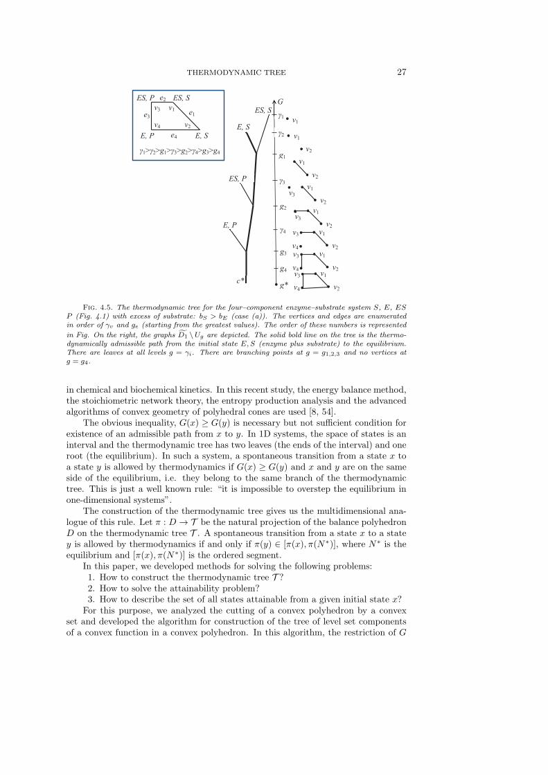
THERMODYNAMIC TREE 27
v4
v3
v2
v1 v4
v3
v3
v3 v2
v1
γ1
γ2
g1
γ3
g2
γ4
g3
g4
g*
v1
v2
v1
v2
v1
v2
v1
v2
2
v1
v4
v4v3
v2
v1
ES, S
E, S
ES, P
E, P
c*
E, P
ES, P
E, S
ES, S
E
v2
v1 v3
P
v4
e1
e2
e4
e3
γ1>γ2>g1>γ3>g2>γ4>g3>g4
G
Fig. 4.5. The thermodynamic tree for the four–component enzyme–substrate system S, E, ESP (Fig. 4.1) with excess of substrate: bS > bE (case (a)). The vertices and edges are enumeratedin order of γv and ge (starting from the greatest values). The order of these numbers is represented
in Fig. On the right, the graphs D1 \Ug are depicted. The solid bold line on the tree is the thermo-dynamically admissible path from the initial state E,S (enzyme plus substrate) to the equilibrium.There are leaves at all levels g = γi. There are branching points at g = g1,2,3 and no vertices atg = g4.
in chemical and biochemical kinetics. In this recent study, the energy balance method,the stoichiometric network theory, the entropy production analysis and the advancedalgorithms of convex geometry of polyhedral cones are used [8, 54].
The obvious inequality, G(x) ≥ G(y) is necessary but not sufficient condition forexistence of an admissible path from x to y. In 1D systems, the space of states is aninterval and the thermodynamic tree has two leaves (the ends of the interval) and oneroot (the equilibrium). In such a system, a spontaneous transition from a state x toa state y is allowed by thermodynamics if G(x) ≥ G(y) and x and y are on the sameside of the equilibrium, i.e. they belong to the same branch of the thermodynamictree. This is just a well known rule: “it is impossible to overstep the equilibrium inone-dimensional systems”.
The construction of the thermodynamic tree gives us the multidimensional ana-logue of this rule. Let π : D → T be the natural projection of the balance polyhedronD on the thermodynamic tree T . A spontaneous transition from a state x to a statey is allowed by thermodynamics if and only if π(y) ∈ [π(x), π(N∗)], where N∗ is theequilibrium and [π(x), π(N∗)] is the ordered segment.
In this paper, we developed methods for solving the following problems:1. How to construct the thermodynamic tree T ?2. How to solve the attainability problem?3. How to describe the set of all states attainable from a given initial state x?
For this purpose, we analyzed the cutting of a convex polyhedron by a convexset and developed the algorithm for construction of the tree of level set componentsof a convex function in a convex polyhedron. In this algorithm, the restriction of G
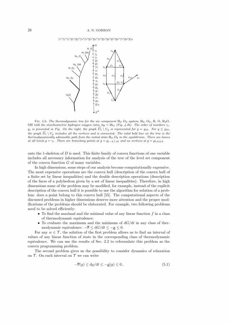
28 A. N. GORBAN
v1
v2
v3
v4
v5
v6
v7
e1
e2 e3
ve4
e5
e6
e7
e8
e9 e10
γ1
γ3 γ3g1
γ4
g3
γ6 γ6g5
g*
G
γ1>γ2>γ3>g1>g2>γ4>γ5>g3>g4>γ6>g5>g6>g7>g8>γ7>g9>g10
γ1γ2
g1g2 γ
γ5 g3g4
g5g6 g6g7 g7g8 g8γ7 γ7g9 g9g10
H, O
H, OH
H2, O
H2, OH
H, O2
H2, O2
H2O
Fig. 4.6. The thermodynamic tree for the six–component H2–O2 system, H2, O2, H, O, H2O,OH with the stoichiometric hydrogen–oxygen ratio, bH = 2bO (Fig. 4.2b). The order of numbers γi,
gj is presented in Fig. On the right, the graph D1 \ Ug is represented for g = g10. For g ≤ g10,
the graph D1 \ Ug includes all the vertices and is connected. The solid bold line on the tree is thethermodynamically admissible path from the initial state H2,O2 to the equilibrium. There are leavesat all levels g = γi. There are branching points at g = g1−4,7,10 and no vertices at g = g5,6,8,9.
onto the 1-skeleton of D is used. This finite family of convex functions of one variableincludes all necessary information for analysis of the tree of the level set componentof the convex function G of many variables.
In high dimensions, some steps of our analysis become computationally expensive.The most expensive operations are the convex hull (description of the convex hull ofa finite set by linear inequalities) and the double description operations (descriptionof the faces of a polyhedron given by a set of linear inequalities). Therefore, in highdimensions some of the problem may be modified, for example, instead of the explicitdescription of the convex hull it is possible to use the algorithm for solution of a prob-lem: does a point belong to this convex hull [55]. The computational aspects of thediscussed problems in higher dimensions deserve more attention and the proper mod-ifications of the problems should be elaborated. For example, two following problemsneed to be solved efficiently:
• To find the maximal and the minimal value of any linear function f in a classof thermodynamic equivalence;
• To evaluate the maximum and the minimum of dG/dt in any class of ther-modynamic equivalence: −σ ≤ dG/dt ≤ −σ ≤ 0.
For any w ∈ T , the solution of the first problem allows us to find an interval ofvalues of any linear function of state in the corresponding class of thermodynamicequivalence. We can use the results of Sec. 2.2 to reformulate this problem as theconvex programming problem.
The second problem gives us the possibility to consider dynamics of relaxationon T . On each interval on T we can write
−σ(g) ≤ dg/dt ≤ −σ(g) ≤ 0 , (5.1)
THERMODYNAMIC TREE 29
where the functions σ(g), σ(g) ≥ 0 depend on the interval on T .
This differential inequality (5.1) will be a tool for the study of the dynamics of re-laxation and may be considered as a reduced kinetic model that substitutes dynamicson the d-dimensional balance polyhedron D by dynamics on the one-dimensional den-drite. The problem of the construction of the reduced model (5.1) is closely related tothe following problem [66]: “Can one establish a lower bound on the entropy produc-tion, in terms of how much the distribution function departs from thermodynamicalequilibrium?” In 1982, C. Cercignani [12] proposed a simple linear estimate for σ(g)for the Boltzmann equation (Cercignani’s conjecture). After that, these estimateswere studied and improved by many authors [15, 11, 65, 66] and now the state of artachieved for the Boltzmann equation gives us some hints how to create the relaxationmodel (5.1) on the thermodynamic tree for the general kinetic systems. This may bethe next step in the study of the thermodynamic trees.
REFERENCES
[1] G. M. Adelson-Velskii, A. S. Kronrod, About level sets of continuous functions with partialderivatives, Dokl. Akad. Nauk SSSR, 49 (4) (1945), pp. 239–241
[2] P. M. Alberti, B. Crell, A. Uhlmann, C. Zylka, Order structure (majorization) and irre-versible processes, in Vernetzte Wissenschaften–Crosslinks in Natural and Social Sciences,P. J. Plath, E.-Chr. Hass, eds.; Logos Verlag, Berlin, Germany, 2008, pp. 281–290.
[3] P. M. Alberti, A. Uhlmann, Stochasticity and Partial Order – Doubly Stochastic Maps andUnitary Mixing; Mathematics and its Applications 9, D. Reidel Publ. Company, Dordrecht-Boston-London, 1982.
[4] V. I. Arnold, On the representability of functions of two variables in the form χ(φ(x)+ψ(y)),Uspehy Math. Nauk, 12 (2) (1957), pp. 119–121.
[5] V. I. Arnold, From Hilbert’s superposition problem to dynamical system, Fields Inst. Comm.,24 (1999), pp. 1–19.
[6] M. L. Balinski, An Algorithm for Finding all Vertices of Convex Polyhedral Sets, SIAM J., 9(1961), 72–88.
[7] A. D. Bazykin, Nonlinear dynamics of interacting populations, World Scientific Publishing:Singapore, 1998.
[8] D. A. Beard, H. Qian, J. B. Bassingthwaighte, Stoichiometric foundation of large-scale bio-chemical system analysis, in Modelling in Molecular Biology, G. Ciobanu and G. Rozenberg,eds.; Springer, Berlin-Heidelberg-New York 1 (2004), pp. 1–21.
[9] V. I. Bykov, Comments on “Structure of complex catalytic reactions: thermodynamic con-straints in kinetic modeling and catalyst evaluation”, Ind. Eng. Chem. Res., 26 (1987),pp. 1943–1944.
[10] L. Boltzmann, Lectures on gas theory, U. of California Press, Berkeley, CA, 1964.[11] E. Carlen, M. Carvalho, Entropy production estimates for Boltzmann equations with phys-
ically realistic collision kernels, J. Statist. Phys., 74 (3-4) (1994), pp. 743–782.[12] C. Cercignani, H-theorem and trend to equilibrium in the kinetic theory of gases, Archiwum
Mechaniki Stosowanej, 34 (3) (1982), pp. 231–241.[13] J.J. Charatonik, Unicoherence and Multicoherence, article f-8 in Encyclopedia of General
Topology, Elsevier, 2003, pp. 331–333.[14] N. V. Chernikova, An algorithm for finding a general formula for nonnegative solutions
of system of linear inequalities, USSR Computational Mathematics and MathematicalPhysics, 5 (1965), pp. 228–233.
[15] L. Desvillettes, Entropy dissipation rate and convergence in kinetic equations. Comm. Math.Phys., 123 (4) (1989), pp. 687–702.
[16] H. Doraiswamy, V. Natarajan, Efficient algorithms for computing Reeb graphs, Computa-tional Geometry, 42 (6-7) (2009), pp. 606–616.
[17] A. Einstein, Strahlungs-Emission und -Absorption nach der Quantentheorie, Verhandlun-gen der Deutschen Physikalischen Gesellschaft, 18 (13/14) (1916). Braunschweig: Vieweg,pp. 318–323.
[18] M. Feinberg, D. Hildebrandt, Optimal reactor design from a geometric viewpoint–I. Uni-versal properties of the attainable region, Chem. Eng. Sci., 52 (1997), pp. 1637–1665.
[19] C. Filippi-Bossy, J. Bordet, J. Villermaux, S. Marchal-Brassely, C. Georgakis, Batch
30 A. N. GORBAN
reactor optimization by use of tendency models, Comput. Chem. Eng., 13 (1989), pp. 35–47[20] A. T. Fomenko, T. L. Kunii, eds., Topological Modeling for Visualization, Springer, Berlin,
1997.[21] K. Fukuda, A. Prodon, 1996. Double description method revisited, in Lecture Notes in Com-
puter Science, vol. 1120. Springer-Verlag, Berlin, 1996, pp. 91–111.[22] J. Gagneur, S. Klamt, Computation of elementary modes: a unifying framework and the
new binary approach, BMC Bioinformatics 2004, 5:175.[23] D. Glasser, D. Hildebrandt, C. Crowe, A geometric approach to steady flow reactors:
the attainable region and optimisation in concentration space, Am. Chem. Soc., 1987,pp. 1803–1810.
[24] A. N. Gorban, Invariant sets for kinetic equations, React. Kinet. Catal. Lett., 10 (1979),pp. 187–190.
[25] A. N. Gorban, Methods for qualitative analysis of chemical kinetics equations, in Numeri-cal Methods of Continuum Mechanics; Institute of Theoretical and Applied Mechanics:Novosibirsk, USSR, 1979; Volume 10, pp. 42–59.
[26] A. N. Gorban, Equilibrium Encircling. Equations of Chemical Kinetics and their Thermody-namic Analysis, Nauka Publ., Novosibirsk, 1984.
[27] A. N. Gorban, P. A. Gorban, G. Judge, Entropy: The Markov Ordering Approach, Entropy,12 (5) (2010), pp. 1145–1193.
[28] A. N. Gorban, B. M. Kaganovich, S. P. Filippov, A. V. Keiko, V. A. Shamansky, I. A.Shirkalin, Thermodynamic Equilibria and Extrema: Analysis of Attainability Regionsand Partial Equilibria, Springer, New York, NY, 2006.
[29] A. N. Gorban, G. S. Yablonskii, On one unused possibility in planning of kinetic experiment,Dokl. Akad. Nauk SSSR, 250 (1980), pp. 1171–1174.
[30] A. N. Gorban, G. S. Yablonskii, Extended detailed balance for systems with irreversiblereactions, Chem. Eng. Sci., 66 (2011), pp. 5388–5399.
[31] A. N. Gorban, G. S. Yablonskii, V. I. Bykov, Path to equilibrium. In Mathematical Problemsof Chemical Thermodynamics, Nauka, Novosibirsk, 1980, pp. 37–47 (in Russian). Englishtranslation: Int. Chem. Eng., 22 (1982), pp. 368–375.
[32] P. M. Gruber, J. M. Wills (eds.), Handbook of Convex Geometry, Volume A, North-Holland,Amsterdam, 1993.
[33] K. M. Hangos, Engineering model reduction and entropy-based Lyapunov functions in chem-ical reaction kinetics, Entropy, 12(4) (2010), pp. 772–797.
[34] D. Hildebrandt, D. Glasser, The attainable region and optimal reactor structures, Chem.Eng. Sci., 45 (1990), pp. 2161–2168.
[35] M. Hill, Chemical product engineering – the third paradigm, Comput. Chem. Eng., 33 (2009),pp. 947–953.
[36] F. Horn, Attainable regions in chemical reaction technique, in The Third European Symposiumon Chemical Reaction Engineering, Pergamon Press, London, UK, 1964, pp. 1–10.
[37] B.M. Kaganovich, A.V. Keiko, V.A. Shamansky, Equilibrium Thermodynamic Modeling ofDissipative Macroscopic Systems, Advances in Chemical Engineering, 39, 2010, pp. 1–74.
[38] S. Kauchali, W. C. Rooney, L. T. Biegler, D. Glasser, D. Hildebrandt, Linear program-ming formulations for attainable region analysis, Chem. Eng. Sci., 57 (2002), pp. 2015–2028.
[39] J. Klemela, Smoothing of multivariate data: density estimation and visualization, J. Wiley& Sons, Inc., Hoboken, NJ, 2009.
[40] A. N. Kolmogorov, Sulla teoria di Volterra della lotta per l’esistenza, Giornale Instituto Ital.Attuari, 7 (1936), pp. 74–80.
[41] F. J. Krambeck, Accessible composition domains for monomolecular systems, Chem. Eng.Sci., 39 (1984), pp. 1181–1184.
[42] A. S. Kronrod, On functions of two variables, Uspechi Matem. Nauk, 5(1) (1950), pp. 24-134.[43] V. I. Manousiouthakis, A. M. Justanieah, L. A. Taylor, The Shrink-Wrap algorithm for
the construction of the attainable region: an application of the IDEAS framework, Comput.Chem. Eng., 28 (2004), pp. 1563–1575.
[44] V. P. Maslov, G. A Omel’yanov,Geometric Asymptotics for Nonlinear PDE. I (Translationsof Mathematical Monographs), American Mathematical Society, Providence, 2001.
[45] R. M. May, W. J. Leonard, Nonlinear Aspects of Competition Between Three Species, SIAMJournal on Applied Mathematics, 29 (1975), pp. 243–253.
[46] C. McGregor, D. Glasser, D. Hildebrandt, The attainable region and Pontryagin’s maxi-mum principle, Ind. Eng. Chem. Res., 38 (1999), pp. 652–659.
[47] M. J. Metzger, D. Glasser, B. Hausberger, D. Hildebrandt, B. J. Glasser B.J. Use ofthe attainable region analysis to optimize particle breakage in a ball mill, Chem. Eng. Sci.,

THERMODYNAMIC TREE 31
64, (2009), pp. 3766–3777.[48] J. Milnor, Morse Theory, Princeton University Press, Princeton, NJ, 1963.[49] T. S. Motzkin, H. Raiffa, G. L. Thompson, R. M. Thrall, The double description method,
in Contributions of the Theory of Games II, H. W. Kuhn and A. W. Tucker, eds., Annalsof Mathematics, 8 (1953), Princeton University Press, Princeton, N.J., pp. 51–73.
[50] H. Nagamochi, T. Ibaraki, Algorithmic Aspects of Graph Connectivity, Cambridge UniversityPress, New York, 2008.
[51] L. Onsager, Reciprocal relations in irreversible processes. I, Phys. Rev., 37 (1931), pp. 405–426.
[52] J. Pearl, R. E. Korf, Search Techniques, Ann. Rev. Comp. Sci., 2 (1987), 451–467.[53] R. Peierls, Model-Making in Physics, Contemp. Phys., 21 (1980), pp. 3–17.[54] H. Qian, D. A. Beard, Thermodynamics of stoichiometric biochemical networks in living
systems far from equilibrium, Biophys. Chem., 114, (2-3), (2005), pp. 213–220.[55] F. P. Preparata, M. I. Shamos, Computational Geometry: An Introduction, Springer, New
York, 1985[56] G. Reeb, Sur les points singuliers dune forme de Pfaff completement integrable ou dune fonc-
tion numerique, Comptes Rendus Acad. Sci. Paris 222 (1946), pp. 847–849.[57] R.T. Rockafellar, Convex Analysis, Princeton University Press: Princeton, NJ, USA, 1970.
Reprint: 1997.[58] S. Schuster, D. A. Fell, T. Dandekar, A general definition of metabolic pathways useful for
systematic organization and analysis of complex metabolic networks, Nat. Biotechnology,18 March (2000), pp. 326–332.
[59] A. I. Shafarevich, Asymptotic solutions of the Navier-Stokes equations and topological in-variants of vector fields. Prandtl–Maslov equations on the Reeb graphs and Fomenko in-variants, Russian J. Math. Phys., 7(2) (2000), pp. 401–447.
[60] R. Shinnar, Thermodynamic analysis in chemical process and reactor design, Chem. Eng.Sci., 43 (1988), pp. 2303–2318.
[61] R. Shinnar, C. A. Feng, Structure of complex catalytic reactions: thermodynamic constraintsin kinetic modeling and catalyst evaluation, Ind. Eng. Chem. Fundam., 24 (1985), pp. 153–170.
[62] K. Sigmung, Kolmogorov and population dynamics, in Kolmogorovs Heritage in Mathematics,
E. Charpentier; A. Lesne, N. K. Nikolski, eds., Springer: Berlin, Germany, 2007; pp. 177–186.
[63] R. L. Smith, M. F. Malone, Attainable regions for polymerization reaction systems, Ind.Eng. Chem. Res., 36 (1997), pp. 1076–1084.
[64] W. Stuetzle, Estimating the cluster tree of a density by analyzing the minimal spanning treeof a sample, J. Classification 20(5) (2003), pp. 25–47.
[65] G. Toscani, C. Villani, Sharp entropy dissipation bounds and explicit rate of trend to equi-librium for the spatially homogeneous Boltzmann equation, Comm. Math. Phys., 203 (3)(1999), pp. 667–706.
[66] C. Villani, Cercignani’s conjecture is sometimes true and always almost true, Comm. Math.Phys., 234 (3) (2003), pp. 455–490.
[67] R. Wegscheider, Uber simultane Gleichgewichte und die Beziehungen zwischen Thermo-dynamik und Reactionskinetik homogener Systeme, Monatshefte fur Chemie / ChemicalMonthly, 32(8) (1911), pp. 849–906.
[68] G. S. Yablonskii, V. I. Bykov, A. N. Gorban, V. I. Elokhin, Kinetic models of catalyticreactions, Comprehensive Chemical Kinetics, Vol. 32, R. G. Compton, ed., Elsevier, Ams-terdam, 1991.
[69] M. Zarodnyuk, A. Keiko, B. Kaganovich, Elaboration of attainability region boundariesin the model of extreme intermediate states, Studia Informatica Universalis, 9 (2011),pp. 161–175.
[70] Ch. Zylka, A note on the attainability of states by equalizing processes, Theor. Chim. Acta,68 (1985), pp. 363–377.


![A Leading UK University | University of Leicester · `z * +*, - . = {' ¦¨§ ¦ / = {' = {' % ]"% =?> @>](https://img.dokumen.tips/doc/110x75/5f36ad447823416cf01d1dfd/a-leading-uk-university-university-of-leicester-z-.jpg)