Embed Size (px)
Citation preview

National travel profiles part B: trips, trends and travel prediction
December 2011
A Milne, S Rendall, S Abley
Abley Transportation Consultants Ltd
NZ Transport Agency research report 467

ISBN 978-0-478-38090-3 (print)
ISBN 978-0-478-38089-7 (electronic)
ISSN 1173-3756 (print)
ISSN 1173-3764 (electronic)
NZ Transport Agency
Private Bag 6995, Wellington 6141, New Zealand
Telephone 64 4 894 5400; facsimile 64 4 894 6100
www.nzta.govt.nz
Milne, A, S Rendall and S Abley (2011) National travel profiles part B: Trips, trends and travel predictions.
NZ Transport Agency research report 467. 94pp.
Abley Transportation Consultants Ltd, PO Box 25 350, Christchurch 8144
This publication is copyright © NZ Transport Agency 2011. Material in it may be reproduced for personal
or in-house use without formal permission or charge, provided suitable acknowledgement is made to this
publication and the NZ Transport Agency as the source. Requests and enquiries about the reproduction of
material in this publication for any other purpose should be made to the Research Programme Manager,
Programmes, Funding and Assessment, National Office, NZ Transport Agency, Private Bag 6995,
Wellington 6141.
Keywords: household travel, New Zealand, school travel, segments, travel behaviour, travel survey, trend,
trip chain, trip complexity, trip rates

An important note for the reader
The NZ Transport Agency is a Crown entity established under the Land Transport Management Act 2003.
The objective of the Agency is to undertake its functions in a way that contributes to an affordable,
integrated, safe, responsive and sustainable land transport system. Each year, the NZ Transport Agency
funds innovative and relevant research that contributes to this objective.
The views expressed in research reports are the outcomes of the independent research, and should not be
regarded as being the opinion or responsibility of the NZ Transport Agency. The material contained in the
reports should not be construed in any way as policy adopted by the NZ Transport Agency or indeed any
agency of the NZ Government. The reports may, however, be used by NZ Government agencies as a
reference in the development of policy.
While research reports are believed to be correct at the time of their preparation, the NZ Transport Agency
and agents involved in their preparation and publication do not accept any liability for use of the research.
People using the research, whether directly or indirectly, should apply and rely on their own skill and
judgement. They should not rely on the contents of the research reports in isolation from other sources of
advice and information. If necessary, they should seek appropriate legal or other expert advice.

Acknowledgements
The authors would like to thank our peer reviewers: David Young, Ian Clark and Lynley Povey for their
timely and thoughtful contributions and comments on issues covered in this research. We also
acknowledge the assistance of Dave Saville in relation to the statistical methods used.
We appreciate the helpful comments of our steering group: Chris Freke (Opus International Consultants)
Bill Frith (Frith Associates) Don Houghton (Houghton Consulting) Jacqueline Blake (NZTA) and Dr Glen
Koorey (University of Canterbury) who provided constructive advice on the project in its formative and
latter stages of reporting.
The authors also wish to recognise the assistance of Andrew Murray, Julie Ballantyne, Grant Smith and
Darren Fiddler for providing feedback and information on strategic transport modelling.
Abbreviations and acronyms
ART Auckland Regional Transport Model
BU business trips
CBD central business district
CTM Christchurch Transport Model
CTS Christchurch Study Transport Model
CV commercial vehicle
DfT Department for Transport, UK
DTLR Department for Transport, Local Government and the Regions, UK
GDP gross domestic product
HBEd home-based education
HBO home-based other
HBSh home-based shopping
HBW home-based work
HIS household interview survey
ITE Institute of Transport Engineers, United States
LCBD lower central business district
LTSA Land Transport Safety Authority (now NZ Transport Agency)
MoT Ministry of Transport, New Zealand
MUA main urban area
NHB non-home-based
NTS National Travel Survey
NZHTS New Zealand Household Travel Survey
NZTA New Zealand Transport Authority
RA rural area
RTA Road Transport Authority, Australia
SUA secondary urban area
TDB Trips Database Bureau, New Zealand
TDM travel demand management
UCBD upper central business district

5
Contents
Executive summary ................................................................................................................................................................. 7
Abstract .......................................................................................................................................................................................... 9
1 Introduction ................................................................................................................................................................ 11 1.1 Background ................................................................................................................... 11 1.2 Research objective ....................................................................................................... 11 1.3 Report structure ........................................................................................................... 12
2 Survey procedure .................................................................................................................................................... 13 2.1 Data description ........................................................................................................... 13 2.2 Weights ......................................................................................................................... 14 2.3 Filters ............................................................................................................................ 15 2.4 Definitions of trips and purposes ................................................................................ 15
3 Literature review ..................................................................................................................................................... 17 3.1 Definition of trip chains and tours .............................................................................. 17 3.2 Existing trip generation resources .............................................................................. 19 3.3 Key trends established from international household travel surveys ....................... 21 3.4 Existing New Zealand strategic transport models ...................................................... 24 3.5 Vehicle ownership ........................................................................................................ 29 3.6 Use of household travel surveys for predictive purposes .......................................... 29 3.7 Summary ....................................................................................................................... 30
4 Trend analysis 2003–10 ...................................................................................................................................... 31 4.1 Treatment of data ........................................................................................................ 31 4.2 Change in trip rates over time ..................................................................................... 32 4.3 Changes in morning departure times ......................................................................... 34 4.4 Mode split of trip chains .............................................................................................. 37 4.5 Trip chain complexity .................................................................................................. 45 4.6 Trip chain duration....................................................................................................... 50 4.7 Travel trends for all purposes ..................................................................................... 53 4.8 Home to education travel ............................................................................................ 54
5 Use of NZHTS data in a predictive context and other uses .......................................................... 61 5.1 Household trip generation ........................................................................................... 61 5.2 Other uses for the NZHTS models ............................................................................... 67
6 Discussion ................................................................................................................................................................... 75 6.1 Trend analysis .............................................................................................................. 75 6.2 Use of NZHTS data in a predictive context ................................................................. 79 6.3 Daily profiling ............................................................................................................... 83
7 Summary and recommendations ................................................................................................................... 84 7.1 Changes in travel behaviour over time ....................................................................... 84 7.2 Travel behaviours in relation to area type .................................................................. 84 7.3 Use of NZHTS data in a predictive context ................................................................. 85 7.4 Applications .................................................................................................................. 86

6
7.5 Recommendations ........................................................................................................ 87
8 References ................................................................................................................................................................... 89
Appendix A: Daily travel profiles ............................................................................................................................... 92

7
Executive summary
This research project extended the work presented in NZ Transport Agency research report 353 ‘National
travel profiles part A: description of daily travel patterns’ (Abley et al 2008), which assessed the trip leg
patterns associated with the 2003–06 New Zealand Household Travel Survey (NZHTS). The earlier work has
now been expanded with the inclusion of four more years of data, analysis of travel in terms of trip chains
and analysis of travel behaviour on the basis of a wider range of area types that distinguish between main
urban areas (MUAs) and the major MUAs of Auckland, Wellington and Canterbury.
The main objective of this research was to maximise the value of the travel information held within the NZHTS.
This was done by examining changes in travel behaviour over time and identifying travel behaviours such as
journey times, trip complexity, mode choice and trip generation rates particular to the area types tested. This
report describes a method used to extract and arrange the NZHTS data into a series of interactive models found
at www.abley.com/NZHTSmodels and at www.nzta.govt.nz/resources/research/reports/467/index.html.
These allow practitioners to quickly undertake a range of enquiries based on user-specified variables such
as car ownership and household compositions to reveal area-specific travel behaviours.
The use of the NZHTS data in a predictive manner was found to be limited for a range of reasons. A key
limitation relates to the fact the data does not contain information that responds to issues affecting future
travel choice such as improvements to public transport, direct changes to fuel prices, traffic congestion or
the relative costs of transport modes. However the manner in which the data has been arranged provides a
useful starting point for explaining current trip generation rates and travel behaviour in response to
changes in demographic structures.
The research revealed that the following changes in travel behaviour had occurred between 2003 and
2010:
• There was some evidence that trips per household had declined over time.
• For the major MUAs of Wellington and Canterbury there was some indication that for the period
between 2003 and 2010, commuters started their morning commute at an earlier time.
• There was no evidence that commuting distances were constantly increasing over time for the major
MUAs in contrast with the other MUAs and SUAs, which did show consistent increases in commute
distances over time.
• Trip durations for drivers in the major MUAs of Wellington and Canterbury had increased during the
period tested.
• Trends showed marginal but consistent increases in vehicle driver mode share for the Auckland MUAs,
while the opposite trend occurred in the Wellington MUAs with no consistent trends in vehicle mode
share observed for the Canterbury MUA.
• There was no consistent pattern of change in trip complexity for the areas tested.
• The Auckland MUAs showed marginal decreases in commute distances over time.
The research revealed the following distinctions in travel behaviours for the different areas tested:
• Higher shares of public transport use were related to larger urban areas.

National travel profiles part B: trips, trends and travel predictions
8
• The major MUA of Wellington had the highest proportion of travel from home to work and education
by public transport and walking.
• The most complex trip chains were associated with travel by motorised forms of transport, particularly
where public transport was used, with the least complex trip chains undertaken as walk trips.
• The major MUA of Wellington showed the highest amount of complex trip chains, which reflected high
public transport use.
• The major MUAs showed higher vehicle driver journey times than the other main and secondary urban
areas, indicating higher levels of congestion in the major centres.
• For pre-school and primary schools, the predominant mode of travel was as a vehicle passenger.
• Cycling to school, while representing a low proportion of trips, was most prevalent in secondary urban
areas (SUAs).
• In the major MUA of Wellington, a quarter of all school-related travel was undertaken by bus, which
was almost double that of the major MUAs of Auckland and Canterbury.
• The variability in mode splits between the areas tested was greatest for non-car-owning households.
Applications
Through the course of this research several new applications of the NZHTS data were identified, including
the development of a school trip generation model and a household person trip generation model
providing a first-cut estimate of person trip rates to a range of destination activities. The NZHTS data can
also be used to profile travel movements by mode throughout the day enabling public transport service
providers to plan services around times of peak demand and assisting transport demand management
(TDM) measures to be directed towards specific road user groups. The findings of this report can also be
used to test a number of conventional wisdoms associated with travel behaviours.
Recommendations
In increasing the value of the NZHTS while preserving the value of continuity within it, the following
potential refinements have been proposed:
• Introduce an enquiry field that asks for reasons why a particular mode of travel was used for journey to
work purposes or alternatively extend the question of parking availability to all transport mode users.
• Explore the potential for supplementary methods of data collection including smart phone
applications that are capable of measuring travel for all transport modes with growing accuracy.
• Amend an existing question to gather journey purpose information from passengers as well as drivers
to assist in determining vehicle occupancy levels.
Future work
An area that would merit further investigation when more data has been collected is public transport
transfer times between trip segments. Such work could reveal transfer penalties and assist public
transport service providers in planning for services that rely upon a series of transfer points to provide

Executive summary
9
service coverage over a wider area. In addition travel behaviour associated with food and non-food
shopping may be significantly different therefore further refinement of the shopping journey purpose may
add additional understanding of shopping trips. Where more data becomes available the models
established in this research can be expanded to include more journey purposes.
Abstract
Using data held within the New Zealand Household Travel Survey (NZHTS), this research examined changes
in travel behaviour between 2003 and 2010 and sought to determine whether travel behaviours such as
journey times, mode choice, trip complexity and trip generation rates differed by area type and region. A
key aim of the research was to unlock further value from the data for the benefit of transport planners and
engineers. The research explored the extent to which NZHTS data could be used in a predictive context
and examined a method to extract and arrange the NZHTS data into a form that would allow practitioners
to quickly undertake a range of enquiries based on user-specified variables such as car ownership and
household compositions to reveal area-specific travel behaviours.
The research provided an additional reference source for policy makers by allowing them to view changes
in travel behaviours over time that might be attributed, in part, to past and present transport policy. The
research findings offer an addition to multi-modal trip generation resources for the benefit of traffic
engineers and can also assist travel planning coordinators to achieve the most effective use of existing
transport resources.

National travel profiles part B: trips, trends and travel predictions
10

1 Introduction
11
1 Introduction
1.1 Background
The New Zealand Household Travel Survey (NZHTS) is a series of travel surveys designed to provide a
databank of personal travel information for New Zealand. It is part of a continuous survey that began in
2003 and is useful in enabling the identification of long-term travel trends. This databank will continue to
be an important source of information for influencing government policies and monitoring transport and
safety performances. The Ministry of Transport (MoT 2007) states ‘the aim of this survey is to increase our
understanding of travel behaviour by people in New Zealand, including travel by car as a driver or
passenger, walking and cycling’. This research analysed NZHTS data recorded between 2003 and 2010.
The continuous survey ensures the availability of up-to-date travel data to formulate new transport and
road safety policies. NZ Transport Agency research report 353 ‘National travel profiles part A: Description
of daily travel patterns (Abley et al 2008) investigated travel behaviour from the NZHTS on a trip leg basis
and recommended further work be undertaken to explore trends in travel behaviour using a larger data
set, arranged in terms of trip chains and with further analysis on a regional basis.
1.2 Research objective
This report is an extension to NZ Transport Agency research report 353. The work undertaken in part A has
been expanded by including four more years of data, and analysing travel in terms of trip chains and on the
basis of more discrete areas of the nation. The main objective of this research was to maximise the value of
the travel information held within the NZHTS database, by arranging the data into an accessible form which
could be used for transportation and regional planning studies and research. In particular, an understanding
of the predictors of travel demand by mode and purpose was sought for a range of variables including car
ownership, region type, area type, year group and household composition.
The intention was, in examining the expected trip rates and mode of travel associated with these variables
on a temporal basis, the capability of the NZHTS data to be used in a predictive context for transportation
planning would be better understood.
The analysis included an examination of the changes in travel over time expressed in trip chains for a
range of journey purposes and modes of travel. It also included a comparison of travel behaviours
between different area types including the major urban areas within Wellington, Auckland and Canterbury
regions as well as other main urban areas (MUAs), secondary urban areas (SUAs) and rural areas (RAs).
The travel behaviours examined included:
• changes in morning departure times
• modes splits for different journey purposes
• trip chain complexity
• trip chain durations
• travel associated with education purposes.

National travel profiles part B: trips, trends and travel predictions
12
The information used within the research related to land use, travel mode and trip purpose relationships
and in particular focused on person and vehicle trip generation at the household level.
The capability of the NZHTS to predict school travel in terms of mode choice and vehicle trip generation
was also examined.
In exploring the predictive capability of the NZHTS data, limitations of the data were identified. This was
intended to assist in highlighting the merits of arranging more targeted questions within the survey to
enhance the value and benefit of future information while maintaining the basic structure of the survey to
ensure comparability with its earlier versions.
As part of increasing awareness of transport issues and making such data more available to professionals,
an output of the research was to arrange the NZHTS data into a form that could be made available
electronically for the benefit of transport practitioners in the regions.
1.3 Report structure
The remainder of this report is structured as follows:
• Chapter 2 explains the NZHTS survey procedure and defines the terms of trip legs, trip purposes and
trip chains.
• Chapter 3 considers the definition of trip chains as established elsewhere and describes existing trip
generation sources. Aspects of New Zealand strategic transport models are also reported along with
the key transport outputs from a small selection of household travel surveys undertaken elsewhere in
the world.
• Chapter 4 examines differences and changes in travel behaviours occurring over time and between
different area types such as major MUAs, other MUAs, SUAs and RAs. The different travel behaviours
for a range of land uses explored include trip chaining behaviour, journey to work departure times,
mode splits for different land uses and trip chain characteristics.
• Chapter 5 explores the use of the NZHTS in a predictive context and examines the use of different trip
production variables such as household type and car ownership for a range of area groupings. This
section also explores the potential use of the NZHTS data as a trip generation model for educational
activities.
• Chapter 6 provides a discussion of the trend analysis and the outputs of the NZHTS models introduced
in the previous section.
• Chapter 7 summarises our conclusions and provides recommendations for the application of our
findings and potential further research.

2 Survey procedure
13
2 Survey procedure
The NZHTS dataset analysed in this report includes travel by approximately 40,000 people from some
22,000 households in sample areas throughout New Zealand between 2003 and 2010. The NZHTS is
administered through an independent contract on behalf of the Ministry of Transport (MoT).
Households are selected and an initial letter is sent from the MoT to each household together with a
pamphlet briefly describing the aims and content of the survey. The interviewer then calls at the address to
gather household information, explain the purpose of the survey, and inform the household which ‘travel
days’ should be diarised. The ‘travel days’ are collected as a 48-hour sample for which the household records
all travel. An even spread by day of week is maintained by systematic allocation of travel days. The survey
includes trips beginning between 4am on the first day to 3.59am on the third day. A memory jogger is left
with the respondents to use for recording travel. Participation in the survey is voluntary.
The households to be sampled are drawn from within randomly selected census meshblocks. Over a five
to seven year period every household within the meshblock will be invited to participate in the survey;
after which a new meshblock will be selected for sampling.
Strategic transport models reflect the expected level of mode change in response to a number of factors.
While the ability of the NZHTS data to be used in a predictive context is limited, there is value in providing
a readily accessible opportunity for people without access to such models to undertake their own analysis
or scenario testing through the models that have been developed as part of this research. The
arrangement of the NZHTS data undertaken as part of this study allows for some limited scenario testing
that provides a starting point for explaining travel behaviour in response to changes in demographic
structures. NZHTS methodology can be found on the MoT website:
www.transport.govt.nz/research/Pages/TravelSurvey-Method.aspx.
2.1 Data description
This research relied on household travel surveys undertaken in 14 local government areas within
New Zealand. Between July 2003 and June 2010, 40,160 people from 21,587 households were interviewed.
The data supplied by the MoT was dated 25 February 2011. In general, the collected data was divided into
the categories shown in table 2.1. This research project only focused on analysing household, person and
trip data to achieve the stated objectives. The variables supplied by the MoT can be found in the
downloads section of the MoT website: www.transport.govt.nz/research/Pages/TravelSurvey-Method.aspx.
National travel profiles part B: trips, trends and travel predictions
14
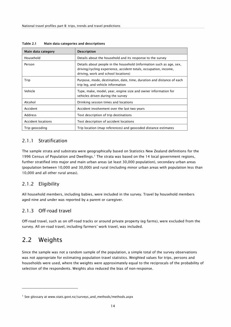
Table 2.1 Main data categories and descriptions
Main data category Description
Household Details about the household and its response to the survey
Person Details about people in the household (information such as age, sex,
driving/cycling experience, accident totals, occupation, income,
driving, work and school locations)
Trip Purpose, mode, destination, date, time, duration and distance of each
trip leg, and vehicle information
Vehicle Type, make, model, year, engine size and owner information for
vehicles driven during the survey
Alcohol Drinking session times and locations
Accident Accident involvement over the last two years
Address Text description of trip destinations
Accident locations Text description of accident locations
Trip geocoding Trip location (map references) and geocoded distance estimates
2.1.1 Stratification
The sample strata and substrata were geographically based on Statistics New Zealand definitions for the
1996 Census of Population and Dwellings.1 The strata was based on the 14 local government regions,
further stratified into major and main urban areas (at least 30,000 population), secondary urban areas
(population between 10,000 and 30,000) and rural (including minor urban areas with population less than
10,000 and all other rural areas).
2.1.2 Eligibility
All household members, including babies, were included in the survey. Travel by household members
aged nine and under was reported by a parent or caregiver.
2.1.3 Off-road travel
Off-road travel, such as on off-road tracks or around private property (eg farms), were excluded from the
survey. All on-road travel, including farmers’ work travel, was included.
2.2 Weights
Since the sample was not a random sample of the population, a simple total of the survey observations
was not appropriate for estimating population travel statistics. Weighted values for trips, persons and
households were used, where the weights were approximately equal to the reciprocals of the probability of
selection of the respondents. Weights also reduced the bias of non-response.
1 See glossary at www.stats.govt.nz/surveys_and_methods/methods.aspx

2 Survey procedure
15
The appropriate weights provided by the MoT in the datasets have been applied in the calculation of all
the travel profiles contained in this research report.
2.3 Filters
‘Filters’ were applied to select households, people and trips by people with full responses only. Filters
applied to the ‘household’, ‘person’ and ‘trip’ datasets provided by MoT are presented in table 2.2.
Table 2.2 Filters used with each dataset
Dataset Filter Description
Household hhrespstat=1 Households with full response only
Person perespstat=1 People in the survey with full responses
Trip perespstat=1 Trips by people with full responses
2.4 Definitions of trips and purposes
The definition and classification of ‘trip legs’, ‘trip chains’, ‘modes’ and ‘trip purposes’ can often vary
between countries. Furthermore, the level at which travel is considered can vary between different
analyses. For example, the Travel survey report 1997/1998 (LTSA 2000) used trip legs to understand
New Zealanders’ travel behaviour, while O’Fallon and Sullivan (2005) used ‘trip chains’. These terms are
defined in the remainder of this section, allowing practitioners to understand how the travel profiles are
generated and to allow comparison with other national and international research.
2.4.1 Trip legs
The trip dataset contains 281,812 rows, each representing a single surveyed trip leg. The MoT defines a
trip leg thus:
A trip leg is a section of travel by a single mode with no stops. Thus if one walks to the bus
stop, catches the bus to town and walks to his/her workplace, he/she has completed three
trip legs (home-bus stop, bus stop 1 to bus stop 2, bus stop 2-work).
2.4.2 Trip leg purpose
Each trip leg has a trip leg purpose; the activity that is performed at the trip leg destination. For this
research, to ensure we considered purposes relevant to the trends being analysed and maintained
sufficient sample sizes, we limited our analysis to the following trip purposes, which in some instances are
combinations of purposes initially coded by the MoT (as stated below):
• Home: where the person is travelling to their permanent or temporary place of residence.
• Employment: these are trip legs to a fixed work address and all work-related stops to other than a
fixed work address. Employed or self-employed people without a fixed place of work (eg plumber) are
included in this category. This is a combination of all the MoT purposes regarding employment (‘work
– main job’, ‘work – other job’ and ‘work – employer’s business’).

National travel profiles part B: trips, trends and travel predictions
16
• Education: this includes travel as a student to institutions such as primary and secondary schools,
colleges of advanced education, technical colleges and universities. It also includes school-related
activities that are not conducted at school, eg school outings, school patrol or sports within school
time. Sports activities during the weekend or after school are coded to recreation. To better
understand travel trends to particular school types, respondent age groupings have been applied to
stratify the responses in some parts of the analysis.
• Shopping: this describes any trip leg ending at premises which sell goods or hire goods out for
money. Premises which provide services only (eg solicitors, banks) or repairs only (eg appliances or
shoe repairs) should be coded as ‘personal business/services’. Shopping is defined as any time the
respondent enters a shop, whether or not a purchase is made.
• Social visits: these include visits to a private home; visits to a non-private dwelling (eg visiting a friend
in hospital, visiting a friend staying in a hotel); pre-school activities such as kindergarten, crèche, day-
care, kohanga reo or nursery school; and all entertainment activities occurring in a public or private
place. Such entertainment activities include dining out, clubs, hotels, concerts, religious meetings, and
off-road driving or motocross. Walking or cycling for social purposes involve exercise and are
therefore coded as ‘recreational’.
• Recreational: this includes participation in sporting activities and travelling to sporting or recreational
activities (eg driving to the park to go jogging). It excludes watching someone else play sport, which is
a ‘social visit’; and off-road driving or motorcycling, which are coded as ‘social visits’ as these have no
exercise component.
• Other: this includes any other trip leg purposes not defined by any of the trip leg definitions above. In
some cases ‘shopping’, ‘social visits’ and ‘recreational’ purposes have all been combined into this
category.
2.4.3 Trip chains
Trip legs, in some cases, are not the most appropriate level at which to understand travel. For some
analyses it is desirable to link travel into trip chains. A trip chain is defined as a series of trip legs where
no stop between legs exceeds a specified time, either 30 or 90 minutes. This research report retains the
90-minute definition of trip chains as used in the Abley et al (2008) report. For example, a trip from work
to home with a stop at shopping for 40 minutes is a trip chain. The main travel purpose of a trip chain is
identified by the purpose of the final chain segment; the travel mode of the chain is defined by the mode
of the segment covering the greatest distance. For example, a trip chain involving walking 500m to a bus
stop, riding the bus 3km to a shop, shopping for 40 minutes then walking 400m to work would have a trip
purpose of work by bus as the main mode.

3 Literature review
17
3 Literature review
A review was undertaken of international literature on trip generation resources, the trends in travel
behaviour derived from household travel surveys and the trip rate inputs to existing strategic transport
models in New Zealand. The function of the literature reviewed in this section is four-fold:
• to clarify the definition of trip, trip legs and trip chains
• to assess the extent and quality of existing trip generation resources available
• to provide a context for travel behaviour trends as established from other household interview surveys
(HIS)
• to explain the key variables and corresponding trip rates used in existing strategic transport models.
The literature review is divided into four parts. The first part is a review of the definition of trips, trip
chains and tours. The second part is a review of existing trip rate databases commonly used in
New Zealand and elsewhere. The third section of the review describes the findings of household travel
survey data found in other countries. The final section describes aspects of transport models developed in
New Zealand which are based on local household travel survey data.
3.1 Definition of trip chains and tours
3.1.1 New Zealand study
O’Fallon and Sullivan (2005) defined a trip chain as ‘a series of one or more segments [trip legs] defined
by starting a new chain whenever:
• the segment [trip leg] is the first one recorded in the respondent’s travel diary (excluding trip legs by
plane)
• the starting point of the segment [trip leg] is home or their workplace
• the origin of the trip is neither home nor work, but the respondent has been at that location for more
than 90 minutes (and the purpose of the immediately preceding segment [trip leg] was not mode
change).’
A trip chain is effectively a one-way trip from an origin to a destination. O’Fallon and Sullivan (2009)
developed the trip chain concept further to define a ‘tour’ as ‘a series of segments [trip legs] that starts
from home and ends at home’ this being a return trip that completes the life cycle of a trip. O’Fallon
classed tours into 10 different types as shown in table 3.1.
Table 3.1 Classification of tours (O’Fallon and Sullivan 2009)
Tour description Sequence
Simple work h-w-h
Multi-part work h-w-(-w-)-w-h
Composite to work h-psl/e-(-psl/w/e-)-w-h
Composite from work h-w(-psl/w/e-)-psl/e-h

National travel profiles part B: trips, trends and travel predictions
18
Tour description Sequence
Composite to and from work h-psl/e-(-psl/w/e-)-w-(-psl/w/e-)-psl/e-h
Composite at work h-w-(-psl/w/e-)-psl/e-(-psl)/w/e-)-w-h
Simple/multi-part education h-e-(e)-h
Composite education and non-work h-psl-e-(-psl-)-h and h-(-psl-)-e-psl-h
Simple non-work/non-education h-psl/ne-h
Multi-part non-work/non-education h-psl-psl-(psl)-h
Where the bracketed terms represent additional segments that may be in the tour, psl is personal travel
(includes personnel business/services, medical/dental and social welfare), shopping and leisure travel
(includes social, leisure and recreational purposes), ie neither work nor education.
The O’Fallon and Sullivan (2009) research reported that respondents in the 2004–07 NZHTS averaged 2.4
trip chains per day, which was a slight increase over the 2.3 trip chains per day calculated on the basis of
the 1997–98 NZHTS.
3.1.2 Australian study
Primerano et al (2007) defined a trip chain to be ‘the linking of secondary activities to a primary activity
through travel that is made from when an individual leaves home to when they return home. It is a
schedule that individuals will follow (or create as they proceed through the day) from the moment they
leave home to the moment they return home’.
Primerano et al (2007) adopted three activities that drive the trip chaining process, which was proposed by
Stopher et al (1996). These activities are classified into three categories:
• mandatory activities, which have frequency (typically daily), location and timing that are all fixed (eg
work and school)
• flexible activities, which are performed on a regular basis but have some characteristics (eg timing or
location) that can vary (eg shopping for convenience goods or banking)
• optional activities, which are discretionary and for which all characteristics may vary. In particular,
frequency may be zero in a given time period (eg social and recreational activities).
It appears the trip chain definition proposed by Primerano et al (2007) is similar to the ‘tour’ defined by
O’Fallon and Sullivan (2005) in that a trip chain starts and ends at home.
3.1.3 US study
The Federal Highway Administration’s operational definition of a trip chain is ‘a sequence of trips bounded
by stops of 30 minutes or less’. A stop of 31 minutes or more defines the terminus of a chain of trips, and
that chain of trips is considered a tour. McGuckin and Nakamoto (2004) used the following definitions to
describe the trip chaining process:
• anchor – a primary or substantial trip destination
• direct trip – a trip that travels directly between two anchor destinations, such as a trip from home to
work

3 Literature review
19
• chain – a series of short trips linked together between anchor destinations, such as a trip that leaves
home, stops to drop a passenger, stops for coffee and continues to work
• intervening stop – the stops associated with chained trips
• tour – total travel between two anchor destinations, such as home and work, including both direct
trips and chained trips with intervening stops. Note that it is possible to have the two anchor
destinations in the same location, as in a home-to-home or work-to-work tour.
3.2 Existing trip generation resources
When travel demand is expressed in terms of trip chains this provides a closer equivalence to trip rates – a
key building block for modelling travel behaviour. When expressed as a trip chain, the NZHTS data can
complement trip generation sources that are currently available to transport practitioners in New Zealand.
There are typically four main international trip generation databases that are used in New Zealand: the
New Zealand Trips, Parking Database Bureau which is now called the Trips Database Bureau (TDB), TRICS®
from the United Kingdom, Roads and Traffic Authority (RTA) of Australia and the Institute of
Transportation Engineers (ITE) Trip Generation of the United States. The features of each of these are
described in the following sections.
The trip rates included in the following databases differ in nature from those commonly used in transport
modelling as the former represent measured arrival and departure movements recorded from empirical
surveys of land-use activities. Trip rates used in transport modelling represent trip attractions and trip
productions measured at the ‘gate’ of development activities. Household trip generation rates can also be
derived from NZHTS data by determining the vehicle trip generation through trip legs:
• grouped by household vehicle ownership
• made by vehicle drivers that originated or terminated at home.
3.2.1 TDB database
The TDB database is a New Zealand-based resource and was first published as Transfund NZ research report
210 (Douglass and McKenzie 2001) ‘Trips and parking related to land use. Volume 2: Trip and parking
surveys database’. This report has been superseded by regular releases and upgrades of the database.
The current TDB database (version August 2010) contains approximately 700 New Zealand sites and 300
Australian sites from the RTA. The information is retained at individual site-by-site levels. The database is
supplied to members as a Microsoft Excel spreadsheet on a CD which is updated annually. Other TDB
research documents, survey methodology, technical notes and similar aids to the understanding of the
database are available on request as well as the website www.tdbonline.org. Typical vehicle trips
associated with residential activities range from 2.6 trips per day for retirement units up to 10.7 trips per
day for large family dwelling houses. Although the type of dwelling and the number of people within a
dwelling are linked, it is the number of people within a household that determines the amount of travel.
3.2.2 TRICS database
The TRICS database is a UK trip generation and parking resource and contains traffic count information for
over 3199 individual sites, 5746 days of survey counts and 110 land-use sub-categories. The database was

National travel profiles part B: trips, trends and travel predictions
20
formed in 1989 and had 301 organisations holding licences when TRICS 2011(a) v 6.7.2 was issued. TRICS
is the most comprehensive database available and now has two versions available. Members of TRICS can
interrogate the database on a site-by-site basis via an online version that can be accessed via the TRICS
website www.trics.org and an offline version that can also be downloaded via the TRICS website. Individual
site details stored in either version can be imported into a Microsoft Excel spreadsheet for further data
manipulation.
New Zealand and Australian members of TDB have ‘inquiry access’ to these TRICS databases through
nominated representatives in each of the main cities. Typical household vehicle trip rates from the TRICS
database range from 1.56 trips for a retirement dwelling and up to 7.6 trips for a dwelling house.
3.2.3 ITE database
The ITE (2008) Trip generation handbook is an American publication and consists of two data volumes
with land-use descriptions, trip generation rates, equations and data plots. Data is included from more
than 4800 sites and 162 land uses. The survey information is merged and analysed together for land-use
groups rather than being retained at an individual site-by-site level. The most recent (8th) edition was
published in 2008. The ITE database is produced in book format and there is also a software version
available. Trip Generation by Microtrans software calculates traffic generation on the basis of the ITE
database and has been updated with each new edition of the ITE report.
Typical household vehicle trip rates from the ITE database range from 2.52 trips for a retirement unit and
up to 9.57 trips for a dwelling house.
3.2.4 RTA database
The RTA database is an Australian publication that contains vehicle trip rates and parking rates
information for nine main land uses. The document only provides an average trip rate by grouped land-use
activities. Site-by-site details of each land-use activity are not included within this document. Many of the
trip and parking rates are based on surveyed data from the 1990s; however, surveys of large bulk retail
stores and senior housing were added in 2009. Collaboration between the TDB and RTA has resulted in
the latest TDB database, dated August 2010, including RTA data.
3.2.5 Multi-modal survey data
Data on modal split and variations between inner, suburban, small town and rural situations is now
deemed of great importance as this supports the national and regional strategies which seek greater
modal integration and increased use of sustainable transport.
One of the most important elements in determining the effects of travel-generating activities is the
collection of relevant data. In most situations where new developments are proposed there will be only
limited sources of information about the particular site or activity. While a major shopping centre, for
example, will generate trip making and parking demand patterns similar to equivalent centres, there will
always be modal split variations and catchment influences which surveys at other sites do not reveal.
In seeking to apply the principles of ‘sustainable transport’, practitioners require an increased awareness
of the contribution to the total transport system of public transport, pedestrian and cycle trips, and the
extent of car passenger as well as car driver travel. More effort is being applied to multi-modal surveys,
which is reflected in current NZTA research such as Pike (2011).

3 Literature review
21
A comparison of the national and the international databases by multi-modal information is shown in
table 3.2.
Table 3.2 Summary of databases by multi-modal information
Database content TDB TRICS ITE RTA
Multi-modal data
available
Yes Yes Light and heavy
vehicle trip rates
only.
Yes
Total number of
surveys
692 3419 4800 192
Number of multi-
modal surveys
90 720 Nil 109
Formal multi-modal
survey methodology
No Yes No No
Surveyed modes Car driver, car
passenger, goods
driver, goods
passenger, pedestrian,
cyclist, bus passenger
Vehicles, pedestrians,
public transport
users, cyclists,
occupants, public
service vehicles,
goods vehicles, taxis
Vehicles and
trucks
Car driver, car
passenger, goods
driver, goods
passenger,
pedestrian, cyclist,
public transport
No. of surveyed
activities (multi-
modal)
12 84 Nil 5
As can be seen from table 3.2 there is still a limited number of New Zealand multi-modal surveys for
informing transport practitioners in New Zealand of modal splits and there is no data on variations of
modal choice over time. While efforts are being made to increase the number of multi-modal survey
results, the database relies upon the good will of transport consultants to offer data they have collected.
This reliance on voluntary contributions explains the slow growth of multi-modal samples within the TDB
database.
3.3 Key trends established from international household travel surveys
The trends established from an analysis of the household travel surveys of other countries provide a basis
of comparison with New Zealand, and changes in travel behaviours observed elsewhere could be a
signpost for changes in New Zealand.
3.3.1 UK National Travel Survey
The UK National Travel Survey (NTS) is a continuous survey of personal travel. The survey is designed to
monitor long-term trends in personal travel in Great Britain. The survey collects information on where,
how, why and when people travel, as well as factors which affect personal travel such as car availability,
driving licence holding and access to key services.
It provides the Department for Transport (DfT), Local Government and the Regions (DTLR) with data to
answer a variety of policy and transport research questions and is used to provide trip rates for the

National travel profiles part B: trips, trends and travel predictions
22
National Trip End Model. The survey has been running continuously since 1988. Like the NZHTS, the NTS
is a travel diary which samples household members over consecutive days.
The DfT produces a series of travel fact sheets periodically that contain key statistics relating to personal
travel. Such data includes details on a range of issues including school travel, car occupancy, commuting
and business travel, and travel in urban and rural areas. The following findings are of key interest for the
purposes of this report:
• Average length of commuting trips increased by 5% between 1995/97 and 2009.
• People in rural locations travel furthest to work.
• Average journey time to work is steadily increasing (18% increase between 1997 and 2009).
• On average: commuting trips by foot take 18 minutes, by cycling 22 minutes, by car 24 minutes and
by bus 41 minutes.
• The average number of trips made per person each year by public transport increases with the size of
the urban area.
• Fewer trips by foot to school occurred in 2008 compared with 1995/97.
• In rural areas more children travel by car or private bus than in urban areas and fewer walk to school
(19%) than the national average (44%).
• There has been a steady falling trend in trip rates since 1995/97. Average distance travelled per
person per year remained relatively stable until 2007, but has declined slightly over the last
three years.
• In 2010, there was an average of 960 trips per person per year – the lowest level since the mid-1970s.
• Between 1995/97 and 2010, overall trip rates fell by 12%. Trips by private modes of transport fell by
14% while public transport modes increased by 8%.
• Most of the decline in overall trips rates between 1995/97 and 2010 can be accounted for by a fall in
the number of trips to shopping and to visit friends.
• Trips by car (as a driver or passenger) accounted for 64% of all trips made and 78% of distance
travelled in 2010.
The 2010 NTS indicated that travel for all trip purposes for all age types averaged 960 trips per person per
year, equating to 2.63 trips per person per day.
3.3.2 The Sydney Household Travel Survey
Household travel surveys are used as inputs to transport and land use planning and policy making at the
regional as well as national level. The Transport Data Centre of New South Wales undertakes a continuous
household travel survey focusing on the greater metropolitan area of Sydney to provide data on current
and future demographic, employment and travel patterns.
Summarising data from the 2009 Sydney Household Travel Survey and journey to work data collected
through the census of population and housing every five years in Australia, it was found that:

3 Literature review
23
• Both residential and employment locations had moved further away from the Sydney central business
district (CBD).
• Public transport share for the journey to work was declining.
• Public transport mode share was around 10% for travel to non-centre locations.
• The average trip length was increasing over time, closely related to the noticeable land use pattern
changes.
• In 2008/09 Sydney residents made 16.3 million trips on an average weekday and 14.7 million on an
average weekend day. Weekday trip growth slowed over the past year to 0.2%, despite population
growth of 1.5% for the same period.
• In the 12 months to 2008/09 there was a growth in public transport and walk trips and vehicle
passengers while the proportion of travel as a vehicle driver declined.
• 54% of respondents cited parking problems as a reason for commuting by public transport
• The drop in car trips was not reflected in levels of household vehicle ownership, which grew at 2.8%.
Despite growth in vehicle ownership, people appeared to be more selective about how often they used
the car.
• Average travel time remained steady. The average time spent travelling each day was 81 minutes per
person. The average duration of a work trip was 34 minutes and the average duration of a non-work
trip was 18 minutes.
The Sydney Household Travel Survey presents data on personal travel expressed as linked trips which is
defined as a journey from one activity to another, ignoring changes of mode and where a linked trip may
comprise one or more unlinked trip legs. Trip rates presented in the Sydney HTS are 3.6 trips per day per
person and 10.2 trips per day per household.
3.3.3 US National Household Travel Survey
The US National Household Travel Survey is undertaken by the Federal Highway Administration in the USA
showing daily vehicle trips per driver of 3.56 trips and person trips of 4.18 trips. Use of regional or state
household travel surveys can reveal travel patterns that are unique to a particular area. The following
example was reported by Milone in a presentation to the Travel Forecasting Subcommittee in 2009 in
relation to the Metropolitan Washington Area Household Travel Survey. In comparing the 2004 and 2009
data for the Washington area Milone reported that:
• within the study area, daily household vehicle trip rates declined from 8.8 to 8.3
• the share of home-based work (HBW) trips, as a percentage of all trips, continued to decline, from 21%
to 18.5%
• the public transport mode share increased from about 6.3% to 7.3%
• car occupancies increased from 1.28 to 1.38
• time-of-day distributions indicated slightly less travel in the peak periods and slightly more midday
travel.

National travel profiles part B: trips, trends and travel predictions
24
A further finding of the US travel survey was that commuting trips (HBW) might not be the dominant
contributor to peak hour traffic demand on the road network. This issue was also highlighted by McGuckin
et al (2005) who supported the proposition, in relation to the survey, that it was the growth of non-work
trips embedded in commute trips that added to traffic congestion during peak times.
3.3.4 Trip complexity
While not a primary output of the household travel survey analyses, trip chain complexity is an important
key output. In their research on travel time competitiveness of cycling in Sydney, Ellison and Greaves cited
many studies that focused on the relationship between trip chain complexity and mode choice. The
general message from the research was that the use of alternative modes was likely to decrease as the
complexity of trip chains increased. Hensher and Reyes (2000) supported this general finding and added
an additional dimension that the complexity of trip chains was likely to increase as a result of an increase
in the number of children and other changes in family structures.
3.4 Existing New Zealand strategic transport models
3.4.1 Wellington
Greater Wellington developed its transport strategy model in 2003 using the 2001 Wellington Region
Household Survey data, timed to align with the 2001 census. The model has been updated to a 2006
basis. The household data comprises three separate files: a household file, a person file and a stop (or
trip) file. Six trip end models (productions and attractions) were produced for the following purposes:
• home-based work (HBW)
• home-based education (HBEd)
• home-based shopping (HBSh) – including personal business
• home-based other (HBO) – combined home-based other and home-based social
• non-home-based other (NHBO)
• business trips (BU) – combining home-based and non-home-based employer’s business
There are different variables within the household survey data that best predict each of the six trip end
models. The final trip rate variables used are summarised in table 3.3.

3 Literature review
25
Table 3.3 Trip end predictors for the Wellington Region Transport Model
Trip end model Production Attraction
HBW Fixed hours Retail employment
Flexible hours Transport & communications employment
Rostered shifts Services employment
Works from home Other employment
Paid employee Manufacturing employment
Self-employed – no others employed Other + manufacturing employment
Self-employed and employer or people Retail + transport & communications + services
employment
Family business
HBEd Primary school age (5–10 yrs) No. of households
Secondary school age (11–16 yrs) No. of households with no tertiary enrolments
Young adult (17–25 yrs) Secondary school enrolments with no tertiary
enrolment
Adult (26+ yrs) Tertiary enrolments
HBSh Children (6–16 yrs) No. of households
Young adult (17–25 yrs) Other employment
Adult (26–65 yrs) Other employment in non-SC sectors
Older adults (66+ yrs) Manufacturing employment
Manufacturing employment in non-SC sectors
Transport & communications employment
Transport & communications employment in non-
SC sectors
Retail employment
Retail employment in non-SC sectors
Retail employment in UCBD sectors
Services employment
Services employment in non-SC sectors
Services employment in UCBD sectors
Services employment in non-SC and non-UCDB
sectors
HBO Children (6–16 yrs) Other employment
Young adult (17–25 yrs) Manufacturing employment
Adults (26–65 yrs) Transport & communications employment
Older adults (66+ yrs) Services employment
With 1 vehicle Retail employment
With 2+ vehicles Retail employment in LCBD (2)
Household size 2+ Retail employment not in LCBD (1)
Household income (000's) Retail employment in UCBD
Retail employment in Petone
Retail employment in LCBD (2)

National travel profiles part B: trips, trends and travel predictions
26
Trip end model Production Attraction
No. of households
No. of households in sector not in LCBD
NHBO Children (6–16 yrs) No. of households
Young adult (17–25 yrs) Retail employment
Adults (26–65 yrs) Retail employment in Petone
Older adults (66+ yrs) Manufacturing employment
Locations not in Wellington city Other employment
With 1 or more vehicles Transport & communications employment
Services employment
BU Fixed hours No. of households
Flexible hours Other employment
Rostered shifts Manufacturing employment
Works from home Transport & communications employment
Part-time workers Services employment
Retail employment
Retail employment in the CBD
Retail + transport & communications employment
Retail + transport & communications employment
in Porirua and Kapiti District
Retail + transport & communications employment
not in Porirua and Kapiti District
non-SC = non-shopping centre
UCBD = upper central business district
LCBD = lower central business district
3.4.2 Auckland
Auckland Regional Council commissioned Sinclair Knight Mertz to develop a regional transport model in
2008 using the 2001 Auckland Region Household Survey data. The household data comprises three
separate files, a household file, a person file and a stop (or trip) file. Six trip end models (productions and
attractions) were produced for the following purposes:
• home-based work (HBW)
• home-based education (HBEd)
• home-based shopping (HBSh)
• home-based other (HBO)
• employer’s business (EB)
• non-home-based other (NHBO).
There are different variables within the household survey data that explain each of the six trip end models.
The variables in each of the production and attraction models are summarised in tables 3.4 and 3.5.

3 Literature review
27
Table 3.4 Trip production variables
Variable HBW HBE HBSh HBO
Employment type �
Work arrangements �
Full-time/part-time �
Person types � � �
Household types � �
Regional growth areas �
Urban/rural � �
Car ownership � � � �
Table 3.5 Trip attraction variables
Variable HBW HBE HBSh HBO
EB
(private
vehicle)
EB
(public
transport)
NHBO
(private
vehicle)
NHBO
(public
transport)
Employment type � � �
Household types �
Educational rolls �
HB attractions (car) � �
HB attractions (public
transport) � �
CBD adjustment � � � � �
Shopping zones �
As part of the process of building the model, extensive work was done to determine the significance or
otherwise that some variables had on trip generation rates. Where variables had little effect these were
combined into more significant variable categories. This reduced the extent of the variables that needed
to be considered. For instance it was found that different household characteristics such as larger
households, or non-working households, or young persons, or older non-working persons all displayed
similar trip rates. Therefore such variables were combined.
Person type and to a lesser extent household type are variables associated with car ownership, which is a
variable that features strongly in all purposes relating to trip production. Person and household types are
also used to a lesser extent as trip production variables. Car ownership effects were found to be more
significant for active modes with active mode trip rates reducing with increasing car ownership.
3.4.3 Christchurch Transport Model
The Christchurch Transport Model (CTM) is a replacement of the vehicle driver-based Christchurch
Transport Study Model (CTS). It is a person-based multi-modal transportation model that includes public
transport passengers and other non-car modes. The model uses household interview survey (HIS) data
collected on the basis of a stratified random sampling procedure by area, the distribution of households
by household type categories and by vehicle availability, and has been subjected to a form of stratified
expansion process.

National travel profiles part B: trips, trends and travel predictions
28
The expansion was initially carried out based on vehicle availability and household type categories
according to the 2006 Census data. Major special generators including the airport and the University of
Canterbury are included in the model. The model adopts a category analysis for trip generations.
The model validation report indicates that as the model reflects total travel, previous difficulties from
vehicle trip rates possibly changing over time were addressed. In the previous CTS model, income as an
explanatory variable for trip generation was investigated but found to be explained by the household and
vehicle categories.
As a refinement to the category-based, trip rate approach, area-specific trip rates were included in the
model to represent proximity to activity areas, or conversely, lower accessibility in rural areas. The model
contains a mechanism for explaining geographic differences in trip rates enabling issues such as the lower
trip rate revealed for certain parts of the district to be incorporated. Following adjustments for under-
reporting in the HIS, the model produced a trip production rate of 12.5 daily person trips per household.
3.4.4 Waikato Regional Transportation Model
The Waikato Regional Transportation Model was the first to be built in New Zealand that included both a
major urban area and an extensive rural area. There was a degree of unease at the outset as to whether
the approach would work, but in the event, there was found to be insufficient difference in the travel
patterns of urban and rural dwellers for separate models to be required.
The model contains the Hamilton, Rotorua, Taupo and Tauranga areas at a coarse level with the Hamilton
area modelled as a four-stage sub-area including public transport, travel demand management (TDM) and
the option of a parking model. The existing models of Rotorua, Taupo and Tauranga remain unchanged
three-step models, except that flows by trip purpose at the boundaries interface with the higher level
regional model.
HIS data was collected by face-to-face interviewers with laptop computers that included custom written
software. Interviewee responses were entered as they were given and the software simultaneously
performed the range and logic tests on the data. This process was said to ensure the integrity of the data,
and was reported as instrumental in removing the need for a correction for under-reporting that was
evident in the Auckland and Christchurch HIS surveys.
The model produced a trip rate of 11.06 person trips per household.
3.4.5 Tauranga Transport Model
For the Tauranga Transport Model, future trip productions are modelled by multiplying the numbers of
households in each category with their trip production rates (which are assumed to remain constant). The
future number of households and people in each area has been estimated by Tauranga City Council. The
number of future trip productions at the model level is made by factoring the base-year car ownership
level with the future car ownership level. For each area, the total number of cars is distributed to future
household numbers in 16 categories, taking into account the change in households, persons per
household and cars per person.
The adopted methodology assumes that growth in vehicle availability is not significantly influenced by
geographic, economic or demographic differences. However, the model builders recognise that higher-
density urban zones positioned near public transport could exhibit lower levels of car ownership than
other areas.

3 Literature review
29
The trip generation models comprise a 24-hour private-vehicle trip production model and trip attraction
model. Trip productions and attractions are produced separately for four trip purposes – home-based
work (HBW), home-based shopping (HBS), home-based other (HBO) and non-home-based (NHB). A separate
model is used to forecast commercial vehicle (CV) generation.
The production model estimates daily trip rates for households classified by car ownership level and
household size. The numbers of households in each category and geographical area are obtained for the
base year from the 1996 Census of Population and Dwellings.
The final daily vehicle trip rates adopted for the Tauranga Transport Model range from 2.8 vehicle trips
per day for one person, one vehicle households up to 11 vehicle trips per day for households with more
than four persons and more than two vehicles available to the household.
3.5 Vehicle ownership
A key variable in the models described above relate to vehicle ownership. In recent research on vehicle
ownership in New Zealand, Conder (2009) reported:
• The number of cars per person increased almost every year between 1970 and 1996.
• Since the 1950s, New Zealand car ownership per person has closely matched Canada and Victoria
(Australia, and was equal to 0.49 cars per person in 1995.
• The average annual changes in cars per person were strongly correlated with changes in GDP per
person and real car prices.
• Auckland had the highest level of vehicles per household in 1996; however, not the highest level of
vehicles per person which was in Nelson/Marlborough.
• Households with a greater number of adults tended to have more vehicles per household.
• Households with retired people tended to have fewer vehicles per household.
3.6 Use of household travel surveys for predictive purposes
As part of the process of establishing trip generation rates for the models described above, different
variable categories are tested to establish the most appropriate trip rates. It is noted here that the level of
disaggregate data used to determine the model trip rates is not available for the NZHTS and therefore
regression has not been done as part of this study.
While the relative disaggregation of the Auckland and Wellington data, which includes some special
variation, does not allow for direct comparisons of trip rates it does provide a useful demonstration of the
significant variables in the Wellington region for trip production and attraction.
The ‘goodness of fit’ for the regression carried out in the Auckland and Wellington modelling
demonstrated the predictive ability of the final selected variables which included the key variables of
household type and availability of a vehicle to the household.

National travel profiles part B: trips, trends and travel predictions
30
As with all transport models, the data used in their construction relates, to some extent, on inputs
collected in the past. Therein lays an inherent assumption that inputs such as trip generation rates remain
valid into the future. While there is little evidence showing changes in person trips over time, UK research
undertaken in 2004 on behalf of TRICS assessed the validity of historic site survey data in relation to
vehicle trip generation.
The research concluded that for some land uses, historic data remained valid while for others this was not
so. The results of the study, which recommended setting cut-off dates for using particular land-use
categories, were applied to the TRICS database. The brief descriptions of the models given in this review
reveal there is some acknowledgement of the potential for change in vehicle trip rates to occur over time
while others assume that vehicle trip rates remain constant.
One significant advantage of the NZHTS is the ability to look at temporal trends both nationally and
regionally to establish changes in travel behaviours over time and to determine the influence that key
variables have on trip rates and transport mode choice.
3.7 Summary
The literature reviewed in this section provided supplementary information regarding trip generation and
travel trends within New Zealand and around the world. Additionally, it provided commentary on the
findings of other household travel surveys and how data from these surveys reflected the trip generation
inputs associated with strategic transport models in New Zealand.
The findings of this literature research were used to guide the selection of the most significant variables
for testing the NZHTS data in a predictive context. The review also provided an understanding of the
definitions of the units of travel for a non modelling audience.
The relevance of the review of the transport models was twofold: first it provided a brief summary of the
models for the understanding of non-modellers and second by reporting the trip generation rates used in
these models (where available), it provided a guide for the person and vehicle trip rates derived from the
analysis of the NZHTS data.
Reference to traffic engineering trip rate resources along with a sample of the range of trip generation
rates associated with residential households provided a point of reference and comparison between the
equivalent trip rates derived from the analysis of the NZHTS data.
The review of international household travel surveys provided useful context in terms of recent personal
travel behaviours and trends in trip making and allowed comparisons between international travel
behaviour and New Zealand. The issues revealed from the international household travel surveys provided
guidance on whether such insights could be gathered from the NZHTS in its current form. By consulting
outputs generated internationally, we were able to ensure both the survey and subsequent analysis of the
results were in line with international methods for investigating travel behaviour.

4 Trend analysis 2003–10
31
4 Trend analysis 2003–10
4.1 Treatment of data
The following analysis was based on trip chains from the data set 2003–10. Trip chains describe how
people link their travel between ‘significant’ locations such as home, work or education, and other
activities. For this report, a trip chain consists of a sequence of segments (trip legs) bounded by stops of
90 minutes or more. The main travel purpose of a trip chain is identified by the purpose of the final chain
segment; the travel mode of the chain is defined by the mode of the segment covering the greatest
distance.
The analysis focused on a comparison of regional areas. The data was separated into the following
discrete groups for comparative purposes:
• MUAs located within the regions of Auckland, Wellington and Canterbury (collectively termed ‘major
MUAs’)
• other MUAs
• secondary urban areas (SUAs)
• rural areas (RAs).
The MUAs located within the regions of Auckland, Wellington and Canterbury were separated from MUAs
located in other regions. This was done in recognition of the fact that while, for example, Wellington city
and Dunedin city are both classified as MUAs, their population and transport infrastructure provision are
significantly different thus potentially resulting in different travel behaviours. The population sizes
associated with MUAs and the urban areas to be included in the MUAs as defined by Statistics New Zealand
are shown in figure 4.1.
Figure 4.1 MUA populations – June 2010
0
50,000
100,000
150,000
200,000
250,000
300,000
350,000
400,000
450,000
500,000
Wha
ngar
ei
North
ern
Auckla
nd zo
ne
Wes
tern
Auc
kland
zone
Centra
l Auc
kland
zone
South
ern
Auckla
nd zo
ne
Hamilto
n zo
ne
Cambr
idge
zone
Te Awam
utu
zone
Taura
nga
Rotor
ua
Gisbor
ne
Napier
zone
Hastin
gs zo
ne
New P
lymou
th
Wan
ganu
i
Palmer
ston
North
Kapiti
Upper
Hut
t zon
e
Lower
Hut
t zon
e
Poriru
a zo
ne
Well
ingto
n zo
ne
Nelson
Christ
chur
ch
Duned
in
Inve
rcar
gill
Area
Po
pu
lati
on
Auckland MUAs
Wellington MUAs
Canterbury MUAs
Other MUAs

National travel profiles part B: trips, trends and travel predictions
32
Although the data is recorded within survey years, the conditions of use stipulate the data must be
aggregated into groups of no smaller than two survey years when reviewing regional trends.
Consequently, the groupings of 2003 through to 2006, 2006 to 2008 and 2008 to 2010 were applied
when assessing changes in travel over time. As the earlier years have fewer samples and the total number
of sample years is uneven the first three years were aggregated. Table 4.1 sets out the sample sizes
associated with each of the groupings.
Table 4.1 Sample sizes
Year grouping 2003–06 2006–08 2008–10
Trips sampled 88,000 57,000 140,000
Trip chains sampled 38,000 24,000 58,000
Trip chains represented* 8,300,000,000 5,700,000,000 5,400,000,000
Household samples 4000 2600 6200
Person samples 11,000 7,000 17,000
* Trip chains represented is the expanded trip chain sample following application of the MoT weightings
It can be seen that the amount of data used to describe the wider population for the 2006–08 period is
lower than in the other year groups. The results established from the other year groups therefore present
higher levels of confidence and may explain instances where outputs associated with the 2006–08 period
sometimes did not follow the general trends established from the other year groups.
For a large part of the analysis, comparisons were made between data that was expressed in proportions
or percentages. For this comparison chi-squared tests were undertaken to determine whether the
differences between the proportions were statistically significant. Where comparisons were made between
values not represented as proportions, t-tests were applied to evaluate the statistical significance. Sample
standard errors were calculated using the bootstrap resampling method with 4000 repetitions. All
differences that had been statistically tested were reported as being either significant or not significant to
the 95th percentile confidence level.
The data was filtered to remove ‘professional driver’ trips, which includes persons such as taxi drivers, as the
inclusion of such trips could bias the output where such an individual may undertake an unrepresentatively
high number of trips. The data was also filtered to remove incomplete survey responses.
The following analysis considers travel behaviour in terms of trip chains. Throughout this report trip
chains are described as trips and should be read as having the same meaning.
4.2 Change in trip rates over time
As set out in chapter 3, household travel surveys have recently recorded declining person and vehicle trip
rates in the UK and vehicle trip rates in the USA and Australia. A significant advantage of the NZHTS is that it
is possible to look at temporal trends to assist in determining whether trip rates are declining in
New Zealand. Figure 4.2 examines daily trip chain rates at the household level, across the major urban areas
for three-year periods.

4 Trend analysis 2003–10
33
Figure 4.2 Temporal analysis of person trip rates per household: 2003–10 within major MUAs
The following observations can be made from figure 4.2:
• In general, and with the exception of the Auckland data corresponding to the 2006–08 period, there
appears to be a decline in trips per household over the period tested. The difference between the
2003 and 2010 periods is significant for all areas.
• The largest decline in trips per household between 2003 and 2010 occurs in the major MUA of
Wellington (13%). The major MUA of Canterbury experiences a net decrease of 9% over the same period.
• The apparent increase in trips for Auckland in the 2006–08 period may be attributed to sampling error.
Figure 4.3 Temporal analysis of person trip rates per household: 2003–10 in other area types
0
1
2
3
4
5
6
7
8
9
2003-06 2006-08 2008-10
Year Group
Tri
p c
hai
ns/
ho
use
ho
ld/d
ay
Auckland
Wellington
Canterbury
0
1
2
3
4
5
6
7
2003-06 2006-08 2008-10
Year Group
Tri
p c
hai
ns/
ho
use
ho
ld/d
ay
Other MUAs
SUAs
RAs

National travel profiles part B: trips, trends and travel predictions
34
The following observations can be made from figure 4.3:
• There is no consistent trend across all area types tested.
• The MUAs display a slight decline then increase over the period tested.
• SUAs show a sharp decline in trips per household before increasing in the period 2006–08 to 2008–10.
• RAs show a continuous decline in trips per household declining 8% between 2003 and 2008, and then
9.5% between 2006 and 2010.
4.2.1 Summary findings of changes in trip rates over time
In general, and with the exception of the Auckland data corresponding to the 2006–08 period, there
appeared to be a decline in trips per household in major MUAs over the period tested.
In relation to the major MUAs, the largest decline in trips per household between 2003 and 2010 occurred
in the major MUA of Wellington (13%). The major MUA of Canterbury experienced a net decrease of 9%
over the same period. The trip rates per household for the other area types did not share a general trend
in the period tested.
4.3 Changes in morning departure times
This analysis explored the morning work departure times of respondents to determine whether there was
any evidence that such trips were occurring earlier, which could be explained by urban sprawl, road
network congestion, or increased trip chaining etc. The analysis, derived by area and specified survey year
groupings, provided the mean, 20th percentile and 80th percentile departure times for the first morning
departure trip to work. Increasing peak spreading would be evidenced as a growing gap between the 20th
and 80th percentiles.
4.3.1 Morning work departure times by vehicles – MUA
Values were mean weighted by trip weights within the sample by the formula shown in equation 4.1. The
expressions used in the formula were taken directly from those provided within the NZHTS data. Only
vehicle trips were counted if the greatest distance segment of the chain was as a vehicle driver or vehicle
passenger.
_1, 11
_1
n tripwgt annidepartureTime departureTimeiArea Year nintripwgt anniin
∑= ⋅=
∑⋅=
(Equation 4.1)
where i…n are the dataset rows for each combination of area and year and mode type.
The pattern of work-related morning departure times for vehicles was established from the above formula.

4 Trend analysis 2003–10
35
Figure 4.4 Temporal analysis of morning work departure time by vehicle within major MUAs
The following observations can be made from figure 4.4:
• Commuters in the Auckland MUAs depart significantly earlier than in the MUAs of Wellington and
Canterbury.
• Commuters in the Canterbury MUA depart at a later time, potentially reflecting the lower levels of
congestion on the road network in this region compared with Auckland and Wellington.
• Between the year groups 2006–08 and 2008–10 all of the MUAs show earlier departure times in
comparison with the departure times associated with the 2003–06 year group.
• Generally, the changes in departure times from one year group to the next are not significant.
• Differences between the departure times of Christchurch and Wellington for all years are not
significant.
• With the exception of the Auckland MUAs in the year group 2008–10, the departure times are
progressively earlier for the other main MUAs.
• Wellington MUAs show the least amount of variation about the mean.
4.3.2 Morning work departure times by all modes – MUA
The data was examined for commuters’ departure time associated with all modes of transport.
06:00
06:28
06:57
07:26
07:55
08:24
08:52
2003-06 2006-08 2008-10 2003-06 2006-08 2008-10 2003-06 2006-08 2008-10
Auckland Wellington Canterbury
Dep
artu
re t
ime
(AM
)
All 80th %ile
mean
All 20%ile

National travel profiles part B: trips, trends and travel predictions
36
Figure 4.5 Temporal analysis of morning work departure time by all modes within major MUAs
A comparison between figures 4.4 and 4.5 indicates there are negligible differences in the departure times
associated with vehicles or all modes of travel. From this comparison it is apparent the departure times
and departure time patterns occurring over time are largely governed by private motor vehicle use.
Therefore, only the departure times associated with home to work trips by vehicle were analysed further.
4.3.3 Morning work departure times by vehicles – other MUA, SUA, rural
Figure 4.6 illustrates the morning work departure times associated with the other area types.
Figure 4.6 Temporal analysis of morning work departure time by vehicle within other area types
06:00
06:28
06:57
07:26
07:55
08:24
08:52
2003-06 2006-08 2008-10 2003-06 2006-08 2008-10 2003-06 2006-08 2008-10
Auckland Wellington Canterbury
Dep
artu
re t
ime
(AM
)
All 80th %ile
mean
All 20%ile
06:00
06:28
06:57
07:26
07:55
08:24
08:52
09:21
2003-06 2006-08 2008-10 2003-06 2006-08 2008-10 2003-06 2006-08 2008-10
Other MUAs SUAs RAs
Dep
artu
re t
ime
(AM
)
All 80th %ile
mean
All 20%ile

4 Trend analysis 2003–10
37
The following observations can be made from figure 4.6:
• Comparison of the three area types shows there is no consistent pattern emerging between them.
• The other MUAs depart later than the SUAs and RAs.
• Departure times associated with the RAs are broadly consistent between each year group, which may
be a function of lower congested routes within the rural road network.
• Generally, the changes in departure times from one year group to the next are not significantly
different.
An analysis of journey times associated with home to work was undertaken for the 2003 to 2010 periods.
While the analysis confirmed work arrival times remained unchanged, the results failed to show any
statistically significant change in the home to work journey time over the period analysed. It was therefore
considered the sample sizes were too small to assert that peak spreading took place.
4.3.4 Summary findings of morning departure times
For vehicle drivers, the start time for the journey to work appeared to be significantly earlier for people
within the Auckland MUAs in comparison with the other area types analysed, which could be attributed to
the more dispersed nature of Auckland and the dominance the car has had in shaping the region to date.
For the Wellington and Canterbury MUAs there was some indication that throughout the period between
2003 and 2010, commuters were starting their morning commute at an earlier time. There was no
evidence to show commuting distances were constantly increasing over time for these MUAs, therefore the
earlier departure times for the Wellington and Canterbury areas may be attributed to higher levels of road
congestion. Journey to work departure times were predominantly related to the vehicle trip as opposed to
other travel modes. Of the area groups tested, the earliest start times were associated with the SUAs and
RAs, potentially reflecting the higher commuting distances for these areas.
4.4 Mode split of trip chains
This section of the analysis examines the mode split of trip chains ending at the following main
destinations:
• employment
• education
• shopping
• social visits
• recreation
• home.
The following analysis examines the mode split of chains by area and year, displayed as the percentage of
weighted trips. The mode for the trip chain is defined as the mode of the trip leg covering the greatest
distance within the chain. The mode splits were derived with the following equation.

National travel profiles part B: trips, trends and travel predictions
38
_1
% 100, , _
1
mtripwgt ann
jnModeDestination Area Year tripwgt ann
i
∑=
= ⋅∑=
where Modej = Mode (Equation 4.2)
and where i…n are the dataset rows for each combination of destination, area and year
The following mode split patterns for the main destinations were established from the above formula.
4.4.1 Mode split of trip chains to employment
Figure 4.7 Mode split of trip chains to employment
The following observations can be made from figure 4.7:
• The predominant mode of travel is by vehicle for each area type.
• Among the main MUAs, Auckland shows the highest share of vehicle drivers (74%) followed by
Canterbury (67%) then Wellington (57%).
• The highest percentages of vehicle drivers can be found in SUAs (83%), RAs (82%) and other MUAs
(79%).
• SUAs display the highest proportion of vehicle driver (83%).
• The difference in the proportion of vehicle passengers between areas is generally statistically
significant, despite being broadly consistent across all area types (7% to 10%).
• Wellington MUAs accommodate the highest share of non-car travel with walking (21%), bus use (6.5%)
and train (6%).
74
67
7983 82
10
8
8
8
87
8
21
16
96 9
57
0 %
10 %
20 %
30 %
40 %
50 %
60 %
70 %
80 %
90 %
100 %
Auckland Wellington Canterbury Other MUAs SUAs RAs
Area type
Per
cen
t o
f T
rip
Ch
ain
s
Other
Bus
Train
Bicycle
Walk
Vehicle Passenger
Vehicle Driver

4 Trend analysis 2003–10
39
• Bus holds 4% mode share for MUAs in both Auckland and Canterbury.
• In the major MUAs Canterbury shows the highest share of bicycle travel (4.9%), followed by Wellington
(1%).
4.4.2 Mode split of trip chains to education
Figure 4.8 Mode split of trip chains to education
The following observations can be made from figure 4.8:
• The predominant mode for education trips in all areas is vehicle passenger.
• Canterbury vehicle driver mode share is more than double that of Auckland and Wellington. This is
probably a consequence of the high number of trips to tertiary education sampled in this region, and
the location of the University of Canterbury within the suburbs, which places it further from denser
residential areas and public transport routes, and the high availability of parking within and around
the campus.
• With the exception of the Canterbury MUA, which shows a vehicle passenger share of 38%, the vehicle
passenger mode share of around 49% is broadly consistent across all other area types.
• With the exception of RAs which show a lower walking share of 12%, a walking share of between 22%
and 26% occurs over all other area types.
• RAs present the highest share of bus use (32%) which is more than double that of any of the other
area types.
• With the exception of the Auckland MUAs where the cycle mode share is less than 1%, cycle mode
share for other area types ranges from 2% to 8%.
9
20
116 7
49 49
3850
49 45
2622
2425
25
12
2
65
8
4
12 1411 8 12
32
9
0 %
10 %
20 %
30 %
40 %
50 %
60 %
70 %
80 %
90 %
100 %
Auckland Wellington Canterbury Other MUAs SUAs RAs
Area type
Per
cen
t o
f T
rip
Ch
ain
s
Other
Bus
Train
Bicycle
Walk
Vehicle Passenger
Vehicle Driver

National travel profiles part B: trips, trends and travel predictions
40
4.4.3 Mode split of trip chains to shopping
Figure 4.9 Mode split of trip chains to shopping
The following observations can be made from figure 4.9:
• The predominant mode share s vehicle driver (46% to 61%).
• RAs present the highest share of vehicle drivers (61%) and the Canterbury MUA shows the lowest
proportion of vehicle drivers (46%).
• The Canterbury MUA presents the highest share of walking (13%).
• In the Wellington MUAs just under 3% of shopping travel is undertaken by train.
• Canterbury enjoys the highest bus mode share (13%). Bus use occurs in all area types.
• Travel by bicycle does not feature highly for shopping trips with the highest use, at 2%, occurring in
SUAs.
• While the differences between the area types for mode of travel as a vehicle passenger are statistically
significant this mode share is comparatively consistent across all area types at around 30%.
55
46
56 5561
2832
30
3027
32
7
5
13
910
4
55
0 %
10 %
20 %
30 %
40 %
50 %
60 %
70 %
80 %
90 %
100 %
Auckland Wellington Canterbury Other MUAs SUAs RAs
Area type
Per
cen
t o
f T
rip
Ch
ain
s
Other
Bus
Train
Bicycle
Walk
Vehicle Passenger
Vehicle Driver

4 Trend analysis 2003–10
41
4.4.4 Mode split of trip chains to social visits
Figure 4.10 Mode split of trip chains to social visits
The following observations can be made from figure 4.10:
• Wellington and Canterbury MUAs have the lowest vehicle driver mode share of 38%.
• While the difference in vehicle driver share between Auckland MUAs and the non-major MUA area groups is
statistically significant, the actual difference between these area groups is slight (46% to 48%).
• Bus use occurs in all area types with the largest bus mode share occurring in the Canterbury MUA (6%).
• The proportion of walk mode is reasonably consistent across all the area types (8% to 11%).
48
38
46 46 47
38
45 42
41 4140
811
11
9 10 10
38
0 %
10 %
20 %
30 %
40 %
50 %
60 %
70 %
80 %
90 %
100 %
Auckland Wellington Canterbury Other MUAs SUAs RAs
Area type
Per
cen
t o
f T
rip
Ch
ain
s
Other
Bus
Train
Bicycle
Walk
Vehicle Passenger
Vehicle Driver

National travel profiles part B: trips, trends and travel predictions
42
4.4.5 Mode split of trip chains to recreation
Figure 4.11 Mode split of trip chains to recreation
The following observations can be made from figure 4.11:
• With the exception of the Canterbury MUA (39%), the mode of vehicle driver is broadly consistent
across all other area types (45% to 47%).
• Bus use is undertaken across all area types ranging from 1% in SUAs to 4% in other MUAs.
• Cycle use occurs across each area type, with maximum cycle use in Canterbury (2.7%).
• Walk mode is consistent among the major MUAs (11% to 12%) and ranges between 9% and 10% for all
other area types.
47
39
45 45 45
34 38
43
4042 41
1211
129
9 10
46
0 %
10 %
20 %
30 %
40 %
50 %
60 %
70 %
80 %
90 %
100 %
Auckland Wellington Canterbury Other MUAs SUAs RAs
Area type
Per
cen
t o
f T
rip
Ch
ain
s
Other
Bus
Train
Bicycle
Walk
Vehicle Passenger
Vehicle Driver

4 Trend analysis 2003–10
43
4.4.6 Mode split of trip chains to home
Figure 4.12 Mode split of trip chains to home
The following observations can be made from figure 4.12:
• The predominant mode of travel to home is by private vehicle.
• The lowest share of private car use occurs in the main MUAs.
• The Canterbury MUA presents the highest proportion of trips by walking (16%).
5653
59 60 60
2626
25
25 24 24
1213
15
12 11 12
54
0 %
10 %
20 %
30 %
40 %
50 %
60 %
70 %
80 %
90 %
100 %
Auckland Wellington Canterbury Other MUAs SUAs RAs
Area type
Per
cen
t o
f T
rip
Ch
ain
s
Other
Bus
Train
Bicycle
Walk
Vehicle Passenger
Vehicle Driver

National travel profiles part B: trips, trends and travel predictions
44
Figure 4.13 Temporal analysis of trip chain mode split to home within major MUAs
The following observations can be made from figure 4.13:
• Comparison between each major MUA reveals there is no common trend in the change of mode split
occurring.
• Over the period 2003–10, the mode share for vehicle drivers increases in Auckland MUAs (55% to 57%)
while Wellington MUAs show a decrease in the share of vehicle drivers (55% to 53%).
• The Canterbury MUA shows a higher mode share for cycling than their Auckland and Wellington
counterparts.
• For the Canterbury MUA, the year group 2006–08 sees a noticeable drop in vehicle driver mode share
although this may be attributed to the lower sample size for this year group.
4.4.7 Key findings of mode split of trip chains
Employment activities generated the highest proportion of vehicle drivers among the land uses tested.
Travel as a vehicle driver was the dominant mode choice for travel to work. For home to work trips, the
largest proportion of vehicle driver mode was associated with the SUAs and RAs reflecting the more
dispersed relationship between residential and employment land use activities in these areas. The lowest
vehicle driver share was found in the major MUAs, with the remaining MUAs showing a significantly higher
share of vehicle drivers for employment purposes, again reflecting the more compact urban forms and
greater choice of alternative ways to travel within those areas located in the major regions.
Education trips in major MUAs showed Canterbury vehicle driver mode share was more than double that of
Auckland and Wellington, which may be a result of the spatial location of the University of Canterbury. It may
have been further influenced by the high number of trips to tertiary education sampled in this region, and
55 56 57 55 54 53 5548
54
27 26 2625 27
2626
24
23
13 12 1212
1314 13
19
15
0 1 12
1 13
43
3 23 3 3 3 3 5 3
0 %
10 %
20 %
30 %
40 %
50 %
60 %
70 %
80 %
90 %
100 %
2003-06 2006-08 2008-10 2003-06 2006-08 2008-10 2003-06 2006-08 2008-10
Auckland Wellington Canterbury
Per
cen
t of
Tri
p C
hai
ns Other
Bus
Train
Bicycle
Walk
Vehicle Passenger
Vehicle Driver

4 Trend analysis 2003–10
45
the availability of parking within and around the Canterbury University campus. The greatest amount of bus
mode share occurred in RAs due to the more dispersed residential locations relative to school locations.
For shopping trips from home, RAs presented the highest share of vehicle drivers, with the Canterbury MUA
showing the lowest proportion of vehicle drivers in comparison with the other area groups tested. The lower
vehicle driver share for Canterbury can be attributed to the higher share of bus use and walking in this area
for shopping purposes. In the Wellington MUAs, just under 3% of home to shopping travel was undertaken by
train. Travel by bicycle did not feature highly for shopping trips with the highest use at 2% occurring in SUAs.
While the differences between the area types for mode of travel as a vehicle passenger were statistically
significant, this mode share was comparatively consistent across all area types at around 30%.
There was significant similarity between mode splits for home to recreation trips and home to social visit
trips which were dominated by travel as a vehicle driver and passenger. Of the land uses investigated,
recreational and social visits attracted the highest proportion of vehicle passengers.
For home-bound travel, which included travel from all journey purposes, the vehicle driver mode share for
the major MUAs was lower in comparison with other MUAs as well as the SUAs and RAs. In general the
mode of travel was broadly consistent across all area types. Trends over time showed marginal but
consistent increases in vehicle driver mode share for the Auckland MUAs, while the opposite trend
occurred in the Wellington MUAs with no consistent trend observed for the Canterbury MUA.
4.5 Trip chain complexity
This section examines the complexity of trip making over time throughout the area types. This is done by
identifying the number of trip legs per chain, and is expressed as a weighted frequency histogram with the
output displayed as a percentage of all trip chains. The analysis is shown first for all trip purposes by year
group, then by work trips.
4.5.1 Change in trip complexity over time for all purposes – major MUAs
Figure 4.14 Temporal analysis of trip chain complexity for all purposes in major MUAs
55 53 54
42 44 4450 49 52
29 31 30
3535 33
31 33 31
10 10 10
14 12 1411 11 11
3 3 45 5 5 5 4 4
0%
20%
40%
60%
80%
100%
2003-06 2006-08 2008-10 2003-06 2006-08 2008-10 2003-06 2006-08 2008-10
Auckland Wellington Canterbury
Per
cen
t o
f tr
ip c
hai
ns
> 4 segments
4 segments
3 segments
2 segments
1 segment

National travel profiles part B: trips, trends and travel predictions
46
The following observations can be made from figure 4.14:
• Small, but statistically significant changes of between 1% and 2% within each of the major MUAs occur
over the year groups.
• Comparisons between each MUA group indicate Wellington MUAs have consistently lower proportions
of one-trip leg trip chains than Canterbury and Auckland MUAs. This difference is statistically
significant.
4.5.2 Change in trip chain complexity over time for all purposes other areas
Figure 4.15 Temporal analysis of trip chain complexity for all purposes in other area types
The following observations can be made from figure 4.15:
• In general, no more than a 2% change occurs between one year group and the next for each of the
above area groups.
• Single leg trip chains represent the predominant trip chain type throughout each non-major area
group.
53 53 53 55 55 54 55 55 57
30 32 3130 29 30 30 31 28
9 9 9 8 9 9 8 7 8
0%
20%
40%
60%
80%
100%
2003-06 2006-08 2008-10 2003-06 2006-08 2008-10 2003-06 2006-08 2008-10
Other MUAs SUAs RAs
Per
cen
t o
f tr
ip c
hai
ns
> 4 segments
4 segments
3 segments
2 segments
1 segment

4 Trend analysis 2003–10
47
4.5.3 Trip chain complexity for all purposes – major MUAs 2003–10
Figure 4.16 Complexity of trip chains for all purposes in major MUAs
The following observations can be made from figure 4.16:
• Auckland MUAs have the highest share of one-leg trip chains (54%) followed by Canterbury (50%).
• Wellington MUAs show the lowest share of one-leg trip chains at 43%.
Length of Trip Chains in Major Urban Areas
54
4350
30
34
31
10
1311
0%
20%
40%
60%
80%
100%
Auckland Wellington Canterbury
Per
cen
t o
f tr
ip c
hai
ns
> 4 segments
4 segments
3 segments
2 segments
1 segment

National travel profiles part B: trips, trends and travel predictions
48
4.5.4 Trip chain complexity for all purposes – other areas 2003–10
Figure 4.17 Complexity of trip chains for all purposes in other area types
The following observations can be made from figure 4.17:
• Single-leg trip chains represent the predominant trip chain type for all area groups.
• RAs display the highest share of one-leg trip chains (56%).
• Variation in trip chain type is no more than 3% for all the area types.
4.5.5 Trip chain complexity and mode choice for all purposes
Table 4.2 Relationship between trip chain complexity and mode choice
Area type
Average number of segments for trip chains by mode
Walk Bicycle Vehicle
driver
Vehicle
passenger Bus & rail
Auckland 1.60 1.47 1.73 1.66 2.67
Wellington 1.75 1.48 1.96 1.85 3.28
Christchurch 1.65 1.44 1.86 1.75 3.06
MUAs 1.63 1.47 1.83 1.78 2.29
SUAs 1.58 1.38 1.79 1.77 1.96
RAs 1.60 1.55 1.78 1.83 1.67
The following observations can be made from table 4.2:
• Bicycle journeys show the least number of trip segments.
Length of Trip Chains
53 55 56
31 29 30
9 8 8
0%
20%
40%
60%
80%
100%
Other MUAs SUAs RAs
Per
cen
t o
f tr
ip c
hai
ns
> 4 segments
4 segments
3 segments
2 segments
1 segment

4 Trend analysis 2003–10
49
• Journeys by public transport show the highest average number of trip legs.
• Trips undertaken as a car driver and passenger are more complex than those undertaken by active
modes.
4.5.6 Home to work trip chain complexity
Figure 4.18 Complexity of trip chains to work in major MUAs
Figure 4.19 Complexity of trip chains to work in other area types
64
46
60
24
32
27
8
15
8
15
3
0%
10%
20%
30%
40%
50%
60%
70%
80%
90%
100%
Auckland Wellington Canterbury
Area type
Per
cen
t o
f tr
ip c
hai
ns
> 4 segments
4 segments
3 segments
2 segments
1 segment
6669 70
2424 21
6 4 5
2 2 2
0%
10%
20%
30%
40%
50%
60%
70%
80%
90%
100%
Other MUAs SUAs RAs
Area type
Per
cen
t o
f tr
ip c
hai
ns
> 4 segments
4 segments
3 segments
2 segments
1 segment

National travel profiles part B: trips, trends and travel predictions
50
The following observations can be made from figures 4.18 and 4.19:
• With the exception of the Wellington MUAs, which show 45% of work trip chains are undertaken as a
one-leg trip chain, all other areas show a higher proportion one-leg trip chains; between 60% and 70%.
• Conversely, Wellington MUAs display the highest proportion of multi-leg trip chains.
• The multi-leg trip chains in Wellington MUAs, of two or more segments, constitute a significantly
higher proportion of trips chains in comparison with the other area types.
• For all area groups, excluding Wellington MUAs, between 20% and 30% of work trip chains consist of
two-leg trip chains.
• The major MUAs show marginally more complex trip chains than other area types.
4.5.7 Summary findings of trip chain complexity
For journeys to work, the proportion of single-segment trip chains is significantly less in Wellington MUAs
than for other area groups. This may be attributed to the higher utilisation of bus and train modes for
journey to work trips in this area.
For all observed area groups, there is no consistency with regard to the direction of change in trip
complexity over time, and the variations that have been observed are no more than 2% of the total.
While less complex trip chains are undertaken by active modes, public transport trip chains are the most
complex, which can be attributed to the necessary segments associated with travelling to and from the
public transport facility.
4.6 Trip chain duration
The following section explores regional and temporal variations in the duration of trip chains, by different
modes. The trip chain times have been examined in minutes for each area type and analysed by year group.
The values are mean weighted by trip weight within the sample by the formula shown in equation 4.3. The
main mode has been identified as the mode by which the greatest distance segment was conducted.
_1, , , 11
_1
n tripwgt anniduration durationiArea Year Mode Destination nintripwgt anniin
∑= ⋅=
∑⋅=
(Equation 4.3)
where i…n are the dataset rows for each combination of area, year and mode.

4 Trend analysis 2003–10
51
4.6.1 Trip chain durations – all area types 2003–10
Table 4.3 Trip chain duration of whole trip (minutes) for all area types 2003–10 average
Area type Walk Bicycle Vehicle driver Vehicle
passenger Bus & rail
Auckland 20.6 30.2 28.6 27.4 55.0
Wellington 24.2 25.5 28.3 27.2 57.7
Canterbury 19.9 27.1 25.5 26.2 46.5
Other MUAs 22.1 23.3 22.7 25.5 58.1
SUAs 22.1 21.6 20.7 25.2 -
RAs 18.8 23.6 26.5 31.8 47.7
'-' indicates that sample size was below the minimum sample size specified by the MoT terms of use for the dataset
The following observations can be made from table 4.3:
• Wellington MUAs show the highest duration for walking trips (24.2 mins) with RAs showing the lowest
duration (18.8 mins).
• There is a wide range of walk durations throughout all area types.
• For modes by vehicle driver the major MUAs within Auckland and Wellington display higher trip
durations than other area types.
• The major MUAs show higher vehicle driver and passenger trip duration than the other main and
secondary urban areas.
4.6.2 Trip chain durations for all purposes – MUAs by year group
Bicycle mode has been omitted from tables 4.4 and 4.5 due to insufficient sample sizes when the data was
broken down into year groupings.
Table 4.4 Trip chain duration for whole trip (minutes) for major MUAs of Auckland, Wellington and
Canterbury regions
Area
Mode
Walk Vehicle driver Vehicle passenger Bus & rail
2003-
06
2006-
08
2008-
10
2003-
06
2006-
08
2008-
10
2003-
06
2006-
08
2008-
10
2003-
06
2006-
08
2008-
10
Auckland 21.2 18.0 22.5 28.8 27.9 28.8 29.4 26.3 25.7 51.3 - 59.6
Wellington 22.6 23.5 26.8 26.5 29.2 30.4 25.6 28.5 28.4 57.2 53.1 62.1
Canterbury 21.3 17.0 21.3 24.8 25.5 26.2 24.3 28.2 26.6 - - 52.9
The following observations can be made from table 4.4:
• Wellington MUAs show the longest duration walk trips in comparison with their Auckland and
Canterbury counterparts.

National travel profiles part B: trips, trends and travel predictions
52
• Auckland and Canterbury MUAs share a pattern of decreasing walk durations, but increasing in 2008–10.
• Trip duration for drivers in the Wellington and Canterbury MUAs increases over the period tested.
• Trip chain durations, in general, are completed within a time budget of between 20 and 30 minutes
for the private transport modes.
4.6.3 Trip chain durations for all purposes – other area types
Table 4.5 Trip chain duration for whole trip (minutes) for other MUAs, SUAs and rural
Area
Mode
Walk Vehicle driver Vehicle passenger Bus & rail
2003-
06
2006-
08
2008-
10
2003-
06
2006-
08
2008-
10
2003-
06
2006-
08
2008-
10
2003-
06
2006-
08
2008-
10
Other
MUAs 21.2 23.6 22.0 22.5 22.0 23.6 25.7 24.2 26.4 65.7 - 58.4
SUAs 20.7 23.7 22.8 21.1 20.9 19.9 25.8 28.6 21.9 - - -
RAs 18.5 17.8 20.4 26.8 26.5 26.0 31.0 34.9 30.1 46.7 44.5 52.2
The following observations can be made from table 4.5:
• RAs show the longest vehicle driver and passenger durations for each year group.
• Trip chain durations for drivers in SUAs decrease over time while trip chain durations for rural drivers
remain relatively static over the period tested.
4.6.4 Trip chain distances for home to work journeys – all area types
Table 4.6 Commute distance (km) by private vehicle (AM peak period)
Year Auckland Wellington Canterbury Other MUAs SUAs RAs
2003–2006 12.74 15.53 9.07 10.35 12.38 19.45
2006–2008 12.31 19.77 8.90 10.89 12.98 17.18
2008–2010 12.14 15.55 10.23 10.97 15.74 17.44
2003–2010 12.44 16.77 9.37 10.69 13.50 18.21
The following observations can be made from table 4.6:
• There is no common direction of change in commuting distances occurring across the area groups.
• The Auckland MUAs show marginal decreases in commute distances over time.
• The lowest average commuting distance is presented by the Canterbury MUA (9.37km) and the highest
commute distance occurs in rural areas (18.21km).
• Of the major MUAs, Wellington shows the highest average commute distance (16.77km).
• Other MUAs and SUAs show consistent increases in commute distance over time.

4 Trend analysis 2003–10
53
4.6.5 Summary findings of trip chain durations
The major MUAs showed higher vehicle driver trip durations than the other main and secondary urban
areas. Trip durations for drivers in the Wellington and Canterbury MUAs increased during the period
tested. Auckland and Wellington MUAs shared a pattern of increased walk and vehicle driver trip chain
durations for the period 2006–08 to 2008–10.
The Auckland MUAs showed marginal decreases in commute distances over time, potentially reflecting
changes in road infrastructure. The lowest average commuting distance was presented by the Canterbury
MUA (9.37km) with rural commute distances representing almost double that of the Canterbury MUA.
Of the major MUAs, Wellington showed the highest average commute distance of around 16km. Other
MUAs and SUAs showed consistent increases in commute distances over time.
4.7 Travel trends for all purposes
This section explores three aspects of travel behaviour for all modes and travel purposes between 2003
and 2010. The aspects explored relate to:
• trip legs per person per year
• travel hours per person per year
• km travelled per person per year.
Equations for these trends are shown in equations 4.4, 4.5 and 4.6:
(Equation 4.4)
where i…n are the dataset rows for each year
(Equation 4.5)
where i…n are the dataset rows for each year
(Equation 4.6)
where i…n are the dataset rows for each year.
1
1
_n
ii
year n
ii
tripwgt annnLegs
peweight
=
=
=∑
∑
1
1
_n
i ii
year n
ii
tripwgt ann distdist
peweight
=
=
⋅=∑
∑
1
1
_n
i ii
year n
ii
tripwgt ann timetime
peweight
=
=
⋅=∑
∑

National travel profiles part B: trips, trends and travel predictions
54
Figure 4.20 Travel pattern changes between 2003–04 and 2009–10
The following observations can be made from figure 4.20:
• Trip legs per person per year peak during the 2005–06 period before declining thereafter. While the
year on year change is not always statistically significant the overall change between 2003 and 2010 is
statistically significant.
• The sharpest decline in all of the travel aspects examined occurs during the period 2006–07.
• Travel hours per person per year peak during the period 2006–07.
• All of the travel aspects have lower values in 2010 than in 2003 with km/person/year seeing the
greatest drop of 9% over the period of analysis.
• Although the hours/person/year statistics show statistically significant changes within the periods
tested, the overall change from 2003 to 2010 is not statistically significant.
• The transport statistics for trip legs per person per year and km per person per year show significant
overall changes between 2003 and 2010.
4.8 Home to education travel
This section examines the travel characteristics associated with education related trip chains, which also
includes trips coded as ‘social visits’ for children under five years of age.
0.00
0.20
0.40
0.60
0.80
1.00
1.20
200304 200405 200506 200607 200708 200809 200910
Survey year
No
rmal
ised
to
200
3-04
yea
r
Trip legs/person/yearhr/person/yearkm/person/year

4 Trend analysis 2003–10
55
4.8.1 Preschool (age group 0–4 years)
Figure 4.21 Preschool modal split of chains for all area types
The following observations can be made from figure 4.21:
• The predominant mode of travel is as a vehicle passenger for all area types.
• Other MUAs show the highest vehicle passenger share (87%) with SUAs showing the lowest proportion
(75%).
• The highest walk share was in Auckland MUAs (17%) followed by Wellington MUAs and SUAs (16%).
• The highest bicycle share can be found in SUAs (3.6%) followed by the Canterbury MUA (1%), with all
other area types showing bicycle use of less than 1%.
• The highest share of bus use can be found in RAs (11%).
80 8285 87
7582
17 16 12 10
167
22 2 3
411
0%
10%
20%
30%
40%
50%
60%
70%
80%
90%
100%
Auckland Wellington Canterbury Other MUAs SUAs RAs
Area type
Per
cen
t o
f tr
ip c
hai
ns Other
Bus
Train
Bicycle
Walk
Vehicle Passenger
Vehicle Driver

National travel profiles part B: trips, trends and travel predictions
56
4.8.2 Primary school (age group 5–10 years)
Figure 4.22 Primary school modal split of chains for all area types
The following observations can be made from figure 4.22:
• The predominant mode of travel is as a vehicle passenger for all area types, ranging from 54% to 73%.
• Other MUAs show the highest proportion of vehicle passengers (73%).
• SUAs and RAs show the lowest proportion of vehicle passenger trips (54% to 57%).
• The highest walk mode of 26% is shared by both Auckland and Canterbury MUAs.
• The highest bus mode share occurs in rural areas (32%) and the lowest bus mode share occurs in the
Canterbury MUA (4%).
• Wellington MUAs present a bus mode share that is three times greater than Auckland MUAs and
double that of the Canterbury MUA.
• With the exception of Auckland, which has a bicycle mode share of less than 1%, bicycle use in all
other area types ranges from 2% to 10%.
6569 67
73
57 54
1726
19
22
11
8 124 5
11
32
26
0%
10%
20%
30%
40%
50%
60%
70%
80%
90%
100%
Auckland Wellington Canterbury Other MUAs SUAs RAs
Area type
Per
cen
t o
f tr
ip c
hai
ns Other
Bus
Train
Bicycle
Walk
Vehicle Passenger
Vehicle Driver

4 Trend analysis 2003–10
57
4.8.3 Intermediate school (age group 10–13 years)
Figure 4.23 Intermediate school modal split of chains for all area types
The following observations can be made from figure 4.23:
• The predominant mode of travel in all area types is as a vehicle passenger.
• The highest walk mode share occurs in the Canterbury MUA (35%) with the lowest walk mode share
occurring in RAs (15%).
• With the exception of Auckland MUAs, which show a bike use of less than 1%, bike use ranges
between 6% for Wellington and up to 15% for other MUAs.
• Bus use is represented in each area type; the lowest share occurs in Wellington and Canterbury MUAs
at 11%.
• The highest bus mode share within the major MUAs is represented by Auckland MUAs (17%), with
Canterbury and Wellington MUAs showing a bus mode share of 11%.
• The highest bus mode share occurs in RAs (35%).
4953
42
49 48
40
32 26
35 2321
15
6 1215
10
10
17 1111
12
21
35
0%
10%
20%
30%
40%
50%
60%
70%
80%
90%
100%
Auckland Wellington Canterbury Other MUAs SUAs RAs
Area type
Per
cen
t o
f tr
ip c
hai
ns Other
Bus
Train
Bicycle
Walk
Vehicle Passenger
Vehicle Driver

National travel profiles part B: trips, trends and travel predictions
58
4.8.4 High schools (age group 13–17 years)
Figure 4.24 High school modal split of chains for all area types
The following observations can be made from figure 4.24:
• The highest share of vehicle driver mode is found in other MUAs (14%) followed by SUAs and RAs at
13%.
• The lowest vehicle driver share can be found in Wellington MUAs (8%), followed by the other major
MUAs within Auckland and Canterbury (10%).
• The highest vehicle passenger mode share can be seen in Auckland (40%).
• The major MUAs show higher vehicle passenger share than other area types.
• There is a large variation in walk mode share, ranging from 14% in RAs to 43% in SUAs.
• Among the major MUAs, walking is the most prominent mode in Canterbury (37%). In Auckland, 28%
of trips are by walking, and in Wellington the figure is 25%.
• Train use occurs in Wellington (5%) Auckland (2.6%) and SUAs (1.5%).
• Cycle use occurs in all areas with Canterbury showing the highest share of 11%, and Auckland MUAs
showing the lowest cycle mode share of 1%.
• Bus use occurs in all areas with RAs representing the highest use of 41% and SUAs the lowest at 9%.
10 8 1014 13 13
40
3426
30 3127
28
25 37
28
43
14
1
2
116
3
4
1425
14
16
9
41
0%
10%
20%
30%
40%
50%
60%
70%
80%
90%
100%
Auckland Wellington Canterbury Other MUAs SUAs RAs
Area type
Per
cen
t o
f tr
ip c
hai
ns Other
Bus
Train
Bicycle
Walk
Vehicle Passenger
Vehicle Driver

4 Trend analysis 2003–10
59
4.8.5 Tertiary education (age group over 18 years)
Figure 4.25 Tertiary education modal split of chains for all area types
The following observations can be made from figure 4.25:
• Vehicle driver is the predominant mode of travel in all areas.
• Between the area types, RAs and SUAs feature the highest percentage of vehicle drivers, while
Auckland and Wellington MUAs feature the lowest.
• The highest walk share of 39% occurs in other MUAs.
• Train use occurs in Wellington MUAs (10%), Auckland MUAs (3.5%) and RAs (1.2%).
• Bicycle use occurs in the Canterbury MUA (4.4%) and other MUAs (2.1%) with other area types showing
less than 1%.
• Bus use is most highly featured in the main MUAs of Auckland (18%) followed by Wellington (15%) and
then Canterbury (14%).
• RAs at 9% represent the highest bus use among the non-major MUA areas.
4.8.6 Summary findings of home to education travel
For pre-school and primary school travel, the predominant mode of travel was as a vehicle passenger for
all area groups. Cycle use within the preschool and primary school age group, while representing a low
proportion of trips, was most prevalent in SUAs.
35
41
4844
59 61
17
11
21
13
2120
25 23
1339
148
18
15 14
26
9
0%
10%
20%
30%
40%
50%
60%
70%
80%
90%
100%
Auckland Wellington Canterbury Other MUAs SUAs RAs
Area type
Per
cen
t o
f tr
ip c
hai
ns Other
Bus
Train
Bicycle
Walk
Vehicle Passenger
Vehicle Driver

National travel profiles part B: trips, trends and travel predictions
60
For the high-school age group, the Auckland MUAs showed a higher dependence upon travel as a vehicle
driver or passenger than all other areas. In the major MUAs of Wellington, a quarter of all education-
related travel was undertaken by bus which was almost double that of the major MUAs of Auckland and
Canterbury. In the major MUA of Canterbury the dominant mode of travel to education was undertaken as
a walk trip.
For school-related education travel, it could be seen that as the age group increased and students became
more travel independent, higher proportions of walk, cycle and bus use occurred.
For the tertiary education sector, travel as a vehicle driver was the dominant mode of travel for all areas.
The Canterbury MUA showed higher levels of car travel both as a driver and passenger than Auckland and
Wellington MUAs. The highest proportion of walk trips for this education group was undertaken by other
MUAs.

5 Use of NZHTS data in a predictive context and other uses
61
5 Use of NZHTS data in a predictive context and other uses
In this section, we report on the use of NZHTS data in predictive models and give an assessment of how
well three key predictor variables relate to household travel. This section also describes, through the
arrangement of the NZHTS data, how it can be used for additional transport planning purposes.
The NZHTS is designed primarily with the concepts of safety and efficiency in mind, rather than as a tool
specifically designed to determine trip generation characteristics of trip making. The ability of the NZHTS
data to be used in a predictive model is limited, first because it is not statistically possible to expand the
data to represent the entire population due to the way in which the sampling is organised, and second
because travel costs are not represented or varied.
Strategic transport models are calibrated against the results of empirical data such as regional-based
household and or roadside interview surveys, public transport on-board surveys, and special generator
surveys which include representative samples of most meshblocks. The NZHTS, in contrast, is based on
data collected on the basis of a stratified cluster sample and as such does not contain the spread of data
required to enable comparisons between models based on alternative data collection techniques to be
easily made.
The relative disaggregation of the input data of strategic transport models also does not allow for direct
comparisons of trip rates to be undertaken with the analysis of the NZHTS which is presented at a more
aggregate level.
The models that are described in the following sections of this report demonstrate the relationship
between age profile, car ownership and household type, with trip generation and mode choice. Additional
variables such as household income, public transport accessibility levels and the perceived cost of
alternative travel modes also have an influence on travel behaviours. Noting that an element of
interrelationship between variables such as income and car ownership occurs, the arrangement of the
NZHTS data as presented in this report assumes all other potential variables and the relativity of travel
costs by mode are equal. The information presented in the following sections therefore represents a
starting point for explaining trip generation and modal choice.
5.1 Household trip generation
Strategic transport models currently have the ability to test the travel effects of changes in a range of
variables. However, access to such models, which do not relate to all locations, is typically limited to the
model proprietors. The models developed for this study provide additional information to practitioners for
a range of area types throughout the country. They also enable various queries to be undertaken that
provide a first-cut assessment of likely changes in travel behaviours based on the key variables used.
In strategic models, person trip rates for each of the categories and dimensions determined during
calibration are usually assumed to be constant over time. However, changes to population demographics
such as an aging population, a shift towards smaller household sizes and adjustments to travel choices
following changes in the availability of carbon-based fuels are all likely to contribute towards changes in
how we travel in the future.

National travel profiles part B: trips, trends and travel predictions
62
Assuming all other potential variables and the relativity of travel costs by mode remain constant,
predictive aspects of the NZHTS data can be established through the arrangement of the data, whereby
users can determine potential changes in trip generation rates and modal splits that may occur as a result
of future changes to demographic structures.
Using the Python programming language to extract data from the NZHTS, a series of models were
established. The models were developed in Microsoft Office Excel enabling practitioners to freely access
the data without the need to develop or purchase specialist modelling software.
The data was arranged to expose the differences in trip chains for each area group during the period
2003–10. The trip chains were expressed as average values with 95% confidence limits shown on the
model outputs.
The data was arranged to show weekday and weekend household trip chains by mode and area types as
used elsewhere in this report, dependent upon the following variables:
• population age profile
• household car ownership
• household type.
In addition to the above, a school travel model was also developed.
5.1.1 Model methodology
The number of trip chains relative to household type was calculated as the sum of trip weights for chains
made by the specified household type within the area, to the destination, divided by the sum of household
weights of specified type within the area, as shown in equation 5.1.
(Equation 5.1)
where i…n are the dataset rows for each combination of household type and area; and j…m are the
dataset rows for each destination.
Trip chains within the selected area are calculated as a product of household type percentage and the
calculated number of trip chains for each destination, as shown in equation 5.2.
(Equation 5.2)
where i…n are the household types.
Overall mode split to the activity destinations is presented in the model output, and represents the mode
split measured within the area to the destination.
The outputs of these equations form the data underpinning the models, samples of which are shown in
tables 5.1 and 5.2. The full complement of data used in each of the models is available for viewing in the
‘Data’ sheet of the relevant spreadsheet model. The data values are weighted by the household type or
1 1, ,
1
_m n
ij i
HouseholdType Area Destination n
ii
tripwgt ann
tripChainshhweight
= =
=
=
∑ ∑
∑
( )( ),
1
%
100
nHouseholdType i
Destination HouseholdType i Destinationi
tripChains tripChains=
= ⋅
∑

5 Use of NZHTS data in a predictive context and other uses
63
vehicle ownership split, which is entered by the user, and then used to determine the resulting trip rate
and modal split.
Table 5.1 Daily weekday person trip rates per household in relation to household composition
Household composition Auckland
MUAs
Wellington
MUAs
Canterbury
MUA
Other
MUAs SUAs RAs
Person alone 2.2 2.6 2 1.9 2 2
Couple 4.6 5.4 4.1 4.4 4.6 3.9
Single parent 6.6 7.1 6.4 6.3 6.2 6.2
Adults 7.4 8.8 7.8 7.3 7.7 6.1
Couple with children 10.3 10 9.6 10.3 10.5 9.0
Table 5.2 Daily weekday person trip rates per household in relation to car ownership
Car ownership per
household
Auckland
MUAs
Wellington
MUAs
Canterbury
MUA
Other
MUAs SUAs RAs
No vehicles 3 2 2 2.2 2 2
One vehicle 5.4 5.1 4.2 3.8 3.8 3.5
Two vehicles 7.5 7.8 7.1 7.2 6.6 5.8
More than two vehicles 10.4 10 9.3 8.5 9.9 7.2
5.1.2 Model inputs
Tables 5.3 to 5.5 summarise the default input values to the model for each of the major urban areas as
they relate to age profile, household type and car ownership profiles. These values were sourced from
Statistics New Zealand based on 2006 Census data. The use of the data for default values enables the
model to broadly reflect existing demographics and hence determine the extent of current household trip
chaining.
Table 5.3 Percentage household car ownership input values (2006)
Percentage household car ownership (2006 Census)
Area Nil 1 2 >2
Auckland 7 35 40 17
Wellington 12 43 34 11
Canterbury 7 37 39 17
New Zealand 8 38 38 16
Table 5.4 Percentage age profiles input values (2006)
Percentage age profile (2006 Census)
Area 0–14 15–19 20–29 30–39 40–49 50–64 65+
Auckland 22 8 14 16 15 15 10
Wellington 21 7 14 15 15 16 11
Canterbury 20 7 13 14 15 17 14
New Zealand 22 7 13 14 15 16 12

National travel profiles part B: trips, trends and travel predictions
64
Total number of households: 2,400 Houshold Vehicle Ownership Split:
No Vehicle 7 %
Area (drop-down menu): One Vehicle 35 %
Two Vehicles 40 %
Three or more Vehicles 18 %
Total 100 %
Auckland
Table 5.5 Percentage household types input values (2006)
Percentage household composition (2006 Census)
Area Person
alone Couple only Adults only
Family with
kids
Single parent
family
Auckland 24 30 7 29 10
Wellington 19 25 10 34 12
Canterbury 25 27 8 29 11
New Zealand 23 27 9 29 12
Figure 5.1 below provides an example screen shot of the input screens for each of the models. The input
screen has been arranged so that through the drop down menu, the user can select the area group of
interest and input the relative variable profiles. The use of the default values as provided in tables 5.3 to
5.5 enables the user to establish the existing number of trips expressed as trip chains per household per
day to various destination activities.
Figure 5.1 Examples of model inputs based on 2006 Census default values
Vehicle ownership
Age profile
Household composition
Auckland Wellington Canterbury Other MUAs SUAs RAs
Total number of households: 2,400 Household Type Split:
Person Alone 25 %
Area (drop-down menu): Couple Only 27 %
Adults Only 8 %
Family with Children 29 %
Single Parent Family 11 %
Total 100 %
Canterbury
Area (drop-down menu):
Age group Split:
0-15 20 % 40-50 15 %
15-20 7 % 50-65 17 %
20-30 13 % 65+ 14 %
30-40 14 % Total 100 %
Canterbury

5 Use of NZHTS data in a predictive context and other uses
65
The different area specific values for car ownership, age profile and household composition reflect some
of the most obvious variables that explain the differences in the extent of travel expressed as trip changes
per household and choice of travel mode within the different area groups identified.
The age variable is different in nature from the other variables tested in that the age profile relates to
person travel rather than household travel. Age profile was selected as a potential variable because it was
thought to have an influence on trip making and given the anticipated aging population of New Zealand, it
was considered that a changing age profile would have an effect on travel patterns in the future. To test
this hypothesis, the age profiles, shown in figure 5.2 and sourced from Canterbury Regional Information
2009 (Canterbury Development Corporation 2009), were used as inputs to the model.
Figure 5.2 Predicted future age profile – Canterbury, source Statistics New Zealand
Although there is predicted to be a doubling of the proportion of people within the retirement age group
by 2031, the model yielded little change in the amount of travel when outputs resulting from the two age
profiles were compared. While age has been shown elsewhere to influence trip making, the models
established from the NZHTS data for this report did not reveal such findings. One possible explanation to
this could be that a significant proportion of 65 year olds remain in work or substitute their previous work
journey for some other journey purpose.
Consequently, the rest of this study focused on variables of car ownership and household composition
that are most typically used as influential factors in transport models when assessing household travel.
To determine the predictive power of household composition and car ownership, an analysis of variance
(Anova) of these variables was undertaken. The car ownership variable is a continuous variable while the
household composition is grouped by its nature. The Anova test revealed that car ownership gave rise to
the largest treatment sum of squares and was therefore the variable with the greatest explanatory power
of the two variables tested.
0
2
4
6
8
10
12
14
16
18
20
0-14 15-19 20-29 30-39 40-49 50-64 65 plus
age group
Per
cen
tag
e ag
e
2006
2031

National travel profiles part B: trips, trends and travel predictions
66
0.0
0.5
1.0
1.5
2.0
2.5
3.0
3.5
4.0
weekda y weekend weekda y weekend weekda y weekend weekda y weekend
Home Employment Educati on Other
Destination Activity
Ho
use
ho
ld T
rip
Ch
ain
s p
er
Da
y
Other
Bus
Train
Bicycle
Vehicle Passenger
Vehicle Driver
Walk
5.1.3 Model outputs
The following example output is based on the Auckland vehicle ownership profile set out in table 5.3.
Figures 5.3 and 5.4 provide example screenshots of the model outputs which represent person trips per
household. Figure 5.3 sets out the overall mode split for the area selected and the number of household
trip chains for the destination activities of home, employment, education and other. Figure 5.4 provides
the same output presented in tabular format. The activities shown in the outputs are those that fall within
the definition of a trip chain terminating when a stop of 90 minutes or more occurs.
Figure 5.3 Model output – Auckland – person trips per household in relation to vehicle ownership
Figure 5.4 Model output – summary table – trips per household per day for Auckland MUAs
Number of Trips: (chains/household/day)
weekday weekend
Home 3.3 2.8
Employment 1.5 0.4
Education 0.8 0.1
Other 1.4 2.3
Total 7.0 5.6
Overall Mode Split: weekday weekend
Walk 16% 8%
Vehicle Driver 50% 49%
Vehicle Passenger 25% 37%
Bicycle 1% 1%
Train 1% 0%
Bus 5% 2%
Other 2% 3%

5 Use of NZHTS data in a predictive context and other uses
67
It can be seen from figures 5.3 and 5.4 that a total person trip rate per household of 7 trips per weekday
and 5.6 trips per weekend is calculated on the basis of the existing car ownership profile for Auckland.
The output in figure 5.4 shows that the current average mode split for person trips to all destinations is
75% as a vehicle driver or passenger.
Were the trip chain to be defined as a stop of 30 minutes or more, rather than the 90-minute definition
currently used, more trip chains would be captured, such as those associated with shopping. The use of a
30-minute trip chain definition would increase the number of trip chains by around 30%.
5.2 Other uses for the NZHTS models
5.2.1 Scenario testing
The model can be used to assess the outcomes of policy goals and transport strategies or external effects
that result in changed travel behaviours. As an example, high car ownership and greenhouse gas emissions
were seen as negative transport issues for Auckland as indicated in its previous long-term plan for a
sustainable city. The plan included targets to address these issues by a variety of measures, such as the
implementation of a sustainable transport programme and the encouragement of active transport modes.
Existing strategic transport models contain projected car ownership rates. Historically, the Auckland
Transport Model ART2 (now ART3) projected very modest changes in car ownership profiles up to 2021 of
no more than 2% change in any of the car ownership categories indicated in figure 5.1. For the purpose of
illustration and assuming the policy initiatives and externalities, such as high fuel costs, have greater
effects, a 5% reduction in vehicle ownership from the higher vehicle owning households and a converse
increase in the number of households associated with lower or nil vehicle ownership can be tested. Such a
change in future vehicle ownership levels may assume the form indicated in figure 5.5.
Figure 5.5 Current and notional future vehicle ownership levels – Auckland
The travel outcomes of changes in car ownership as indicated in figure 5.5 could be assessed using the
model to reveal travel demand and mode choice changes as indicated in figures 5.6 and 5.7.
0
5
10
15
20
25
30
35
40
45
0 1 2 >2
Cars per Household
%ag
e H
ou
seho
ld C
ar o
wn
ersh
ip
Existing Car Ow nership
Future Car Ow nership

National travel profiles part B: trips, trends and travel predictions
68
Figure 5.6 Model output - travel behaviour based on notional future vehicle ownership profile – Auckland
MUAs
Figure 5.7 Model outputs - travel behaviour based on notional future vehicle ownership profile – Auckland
MUAs
By comparing the model outputs in figure 5.3 and 5.4 against those shown in 5.6 and 5.7, it can be seen
that as a result of notional future vehicle ownership profile, a measurable reduction in person trips per
household and an increase in use of more sustainable forms of transport would be expected.
While the above example is based on a notional future car ownership profile, such input data could be
obtained from a range of sources including those authorities that possess their own strategic land-use and
transportation models.
0.0
0.5
1.0
1.5
2.0
2.5
3.0
3.5
weekday weekend weekday weekend weekday weekend weekday weekend
Home Employment Education Other
Destination Activity
Ho
use
ho
ld T
rip
Ch
ain
s p
er
Da
y
Other
Bus
Train
Bicycle
Vehicle Passenger
Vehicle Driver
Walk
Number of Trips: (chains/household/day)
weekday weekend
Home 3.1 2.6
Employment 1.3 0.3
Education 0.7 0.0
Other 1.4 2.2
Total 6.5 5.2
Overall Mode Split: weekday weekend
Walk 18% 9%
Vehicle Driver 47% 47%
Vehicle Passenger 25% 38%
Bicycle 1% 1%
Train 1% 0%
Bus 6% 2%
Other 2% 3%

5 Use of NZHTS data in a predictive context and other uses
69
5.2.2 Discrete analysis
The models can be used to examine the person trip per household in relation to demographic groups for
each area tested. The models contain a significant amount of information, covering six area types,
weekday and weekend samples over a range of household types or ownership levels as well as background
information such as sample sizes and statistical measures.
The values set out in tables 5.1 and 5.2 represent average daily person trips per household. To determine
the trip rate for a specific area, the demographic structure of that area would need to be known in order to
weight the values in tables 5.1 and 5.2 appropriately. However in the format presented, it can be seen that
in general there are differences between each area for the same variable.
In comparing the main MUAs with the other MUAs it can be seen that the number of trip chains per
household, in general, tends to be lower for the other MUAs. This finding suggests that applying main
MUA trip rates to other MUA areas would generally overestimate trip rates, in the absence of some
adjustment factor to reflect local conditions.
The use of a single category, such as vehicle ownership or household composition, will explain some of
the variation in the number of trips generated per household. The use of multiple variables whereby trip
rates are determined on the basis of ‘x’ number of people with ‘y’ number of cars available to the
household can improve the predictive ability of a model. However the ability to do this with the NZHTS
data is limited due to the low sample sizes available at this disaggregate level.
The model can be used to examine mode splits for a particular demographic group for each area tested.
As an example, figure 5.8 shows the mode splits for Auckland households with nil vehicle ownership.
Figure 5.8 Example of model output – Auckland households with nil vehicle ownership
It can be seen in figure 5.8 that fewer trips were undertaken for this group in comparison with the model
output shown in figure 5.3 which included car-owning groups. The lower trip rates for the non-car owning
households indicated that car ownership influenced not only the choice of transport mode but also the
amount of travel per household.
Other comparisons between the car-owning and non-car-owning groups show that for the non-car-owning
households the proportion of trips as a car passenger was higher, as was the share of walking trips. The
0.0
0.5
1.0
1.5
2.0
2.5
3.0
weekday weekend weekday weekend weekday weekend weekday weekend
Home Empl oyment Educati on Other
Destination Activity
Ho
use
ho
ld T
rip
Ch
ain
s p
er
Da
y
Other
Bus
Train
Bicycle
Vehicle Passenger
Vehicle Driver
Walk

National travel profiles part B: trips, trends and travel predictions
70
output also shows there was a more pronounced difference between travel modes for weekday and
weekend in the non-car-owning households.
A summary of the effects of car ownership on the level of use of walking, cycling and bus is set out in
table 5.6.
Table 5.6 Comparison of weekday percentage mode split in relation to household car ownership
Area type O cars 1 car 2 cars 3 or more cars
walk cycle bus walk cycle bus walk cycle bus walk cycle bus
Auckland 54% 4% 19% 17% 0% 6% 11% 0% 4% 9% 0% 3%
Wellington 33% 0% 36% 19% 1% 7% 13% 1% 4% 13% 2% 3%
Christchurch 42% 8% 29% 19% 4% 6% 15% 4% 3% 10% 2% 3%
MUAs 53% 7% 11% 15% 2% 2% 9% 2% 1% 7% 3% 2%
SUAs 45% 16% 2% 16% 2% 3% 8% 3% 2% 7% 3% 2%
RAs 53% 2% 17% 16% 2% 5% 9% 2% 5% 7% 1% 5%
It can be seen in table 5.6 that the greatest change in mode splits occurs between the non-car-owning
households and those with a car. The differences in mode split among those households with access to a
car are less pronounced. Of the sample tested, the standout statistics are that zero-car households in the
major MUA of Wellington show no use of a bicycle while similar households in other areas such as SUAs
showed as much as 16% cycle share. The data also shows that car-owning households in the major MUA of
Auckland make almost no cycle trips.
5.2.3 School travel profiling
The NZHTS data can also be arranged to assess the multi-modal trip generation associated with school
travel. As well as travel by students, travel associated with schools also includes trips by service people
and staff. These two groups are not identified within the NZHTS, and therefore require additional
consideration in the school travel model.
Service people such as plumbers or technicians may travel to school as part of their business. These types
of travel would be coded as ‘work-employer’s business’, although it is not possible to determine their
association with particular education facilities. However, use of UK education trip data sourced from
TRICS, shows that service vehicles represent no more than 1% of the total daily flows to education
facilities. Supported by the recent NZ Transport Agency research report 438 (O’Fallon and Sullivan 2011),
indicating that trip generation characteristics in the UK and New Zealand are very similar for a range of
land uses, it is reasonable to assume a similar service vehicle proportion could generally be expected with
New Zealand education facilities.
Teacher or staff travel to school would be coded in the NZHTS as ‘work-main job’ or ‘work-other job’.
However, the survey does not consistently specify the type of employment, or the location type.
Consequently, this proportion of trips must be assumed by applying the national teacher/pupil ratio of
1:20 to the number of students at the school and assuming that staff travel in single occupant vehicles.
Following the inputs of the area group, school type and enrolment number, the model user is presented
with trips by mode as indicated in figures 5.9 and 5.10.

5 Use of NZHTS data in a predictive context and other uses
71
Figure 5.9 Example model output – summary trip generation – 300 pupil high school main urban areas
Figure 5.10 Example model output – summary trip generation – 300 pupil high school main urban areas
The above summary table can be used to assist school travel planners identify age groups within certain
locations that could benefit the most from school travel plan initiatives. For instance, it can be seen that
effort can be directed at the major urban areas to maintain and enhance travel by walking and bus
between the 11 to 12 and the 13 to 17 age groups. The vehicle trip generation outputs can also be used
to assess the traffic impacts of a particular school for both the morning and afternoon peak periods.
0
50
100
150
200
250
300
Walk Cycle P.T. V. Driver V. Pass. Taxi Other
Mode
Tri
ps
by
Mo
de
Arriva ls
Deaprtures
Total daily student trips: 918 arrivals + departures
Students by Mode of Travel - Arrivals
Walk Cycle P.T. V. Driver V. Pass. Taxi Other
Mode Split (%) 30.4 5.2 16.2 14.7 29.0 0.5 4.0
No. of Students by Mode 91 16 49 44 87 1 12
Trips by Mode 139 24 74 68 133 2 18
Students by Mode of Travel - Departures
Walk Cycle P.T. V. Driver V. Pass. Taxi Other
Mode Split (%) 35.0 5.5 17.2 15.1 22.4 0.8 4.1
No. of Students by Mode 105 16 52 45 67 2 12
Trips by Mode 160 25 79 69 103 4 19
School Trips undertaken by Private Motor Vehicles
Arrivals Departures
Student Passenger Vehicle Trips 107 84 Including taxi passengers.
Student Driver Vehicle Trips 68 69
Staff Trip Legs 15 15 One staff member per 20 students; all drive.
Service Vehicle Trips 1 1 Service vehicles represent 1% of total daily flows.
Total Daily Vehicles 359 Vehicles
Peak Hour Private Motor Vehicles
AM Peak (8AM to 9AM) 129 Vehicles
PM Peak (3PM to 4PM) 98 Vehicles

National travel profiles part B: trips, trends and travel predictions
72
5.2.4 Daily vehicle trips and travel profiling
The NZHTS data can also be arranged to reveal daily vehicle trips per household calculated on the basis of
vehicle ownership, and determining the vehicle trip generation by arranging trip legs made by vehicle
drivers that originated or terminated at the home, grouped by household vehicle ownership. Figure 5.11
shows the vehicle trip rates associated with the identified area groups.
Figure 5.11 Household vehicle trip generation (vehicle driver trips to and from home) based on car ownership
As indicated in the previous sections, higher car ownership results in a greater number of vehicle trips
being undertaken per household. Figure 5.11 supports this finding in terms of vehicle trip generation,
showing vehicle trip rates ranging from zero trips per day per household to nine trips per day per
household. These trip rates relate to all household types ranging from retirement units to large family
dwellings. The values in figure 5.11 represent minimum vehicle trips and do not include vehicle trips to
and from households that are associated with visitors, household members as passengers in non-
household cars and service vehicles.
Table 5.7 presents an alternative way to express household trip making in terms of person trip legs and
person trip chains per household, which includes travel by all modes.
Table 5.7 Average weekday person trip rates per household
Area type Average weekday person-trip-
legs/household/day
Average weekday person-trip-
chains/household/day
Major MUA Auckland 15.5 7.1
Major MUA Wellington 16.8 6.7
Major MUA Canterbury 13.0 5.6
MUAs 12.8 5.6
SUAs 13.1 5.9
RAs 12.3 5.3
0
2
4
6
8
10
0 1 2 3+
Household Vehicle Ownership
Dai
ly v
ehic
le d
rive
r tr
ip g
ener
atio
n (
in +
ou
t)
Auckland
Wellington
Canterbury
Other MUAs
SUAs
RAs

5 Use of NZHTS data in a predictive context and other uses
73
It can be seen in table 5.7 that the major MUA of Auckland displays the highest number of daily trip chains
followed by the major MUA of Wellington. However, in Wellington a greater number of daily trip legs are
undertaken, which indicates more complex trip chains and concurs with the previous findings of this report.
In addition to providing travel patterns over periods of years, the NZHTS can also be used to examine the
pattern of travel throughout the day for different journey purposes and travel modes. The daily travel
profiles for SUAs and the major MUA of Canterbury are shown in figures 5.12 and 5.13; profiles for all
regions are contained in appendix A. To reduce the effects of rounding in the responses the output has
been smoothed using a 60-minute window.
Figure 5.12 Daily travel profile – road users – secondary urban areas
Figure 5.13 Daily travel profile – road users – Christchurch major urban area
0.0%
0.5%
1.0%
1.5%
2.0%
2.5%
0 4 8 12 16 20 24
Hour
Per
cen
t o
f tr
ips
Other
Employment
Home
0.0%
0.5%
1.0%
1.5%
2.0%
2.5%
3.0%
0 4 8 12 16 20 24
Hour
Per
cen
t o
f tr
ips
Other
Employment
Home

National travel profiles part B: trips, trends and travel predictions
74
As the examples in figures 5.11 and 5.12 show, there are basic similarities between the travel profiles for
the different areas. Both figures reveal relatively similar daily travel profiles, showing the build up and
decrease in travel demand throughout the day for various activities with identifiable peak periods.
However, the two profiles do contain some quite distinct differences. For instance, travel to employment
constituted a higher proportion of the travel during the morning peak period (between 6am and 9am) in
SUAs than in the Canterbury MUA. This would indicate the implementation of workplace travel plans in SUAs
would have a greater effect on easing congestion. Other observable differences are higher peaks and a
greater proportion of travel to other activities in the MUA. The outputs for the other major MUAs, and
interestingly RAs, display similar characteristics to those seen in the major MUA of Canterbury.

6 Discussion
75
6 Discussion
This section of the report reflects upon the findings of the analysis in the context of the project brief and
the findings of the literature review. The aims of this project were to maximise the value of the travel data
in the NZHTS and extend the analysis of the NZHTS reported in NZ Transport Agency research report 353
(Abley et al 2008) by exploring recent trends in travel behaviour using a larger data set, arranged in terms
of trip chains, and undertaking further analysis on a regional basis. The analysis included an examination
of the changes in travel over time expressed in trip chains for a range of journey purposes and modes of
travel and provided a comparison of travel behaviours between different area types including the major
urban areas of Wellington, Auckland and Canterbury as well as other area types including main urban
areas (MUAs), secondary urban areas (SUAs) and rural areas (RAs).
6.1 Trend analysis
6.1.1 Changes in trip rates over time
As reported in chapter three, there has been a steadily falling trend in trips per person per year in the UK.
This decline is attributed to lower shopping and recreation trips and could also be caused by smaller
household sizes, and from 2008 onwards, the potential effects of the global economic crisis. Additionally
household vehicle trip rates have declined in the USA and Australia in recent years.
The analysis of changes in household trip rates in New Zealand during the period 2003 to 2010 was less
conclusive. The trip rates associated with the 2006–08 Auckland data appeared to be uncharacteristic in
comparison with the other major MUAs of Wellington and Canterbury. It is unknown whether this was due
to sampling errors exacerbated by the lower sample size associated with the 2006–08 period, or simply
reflected the scale of variation that could be expected between one year group and another.
In spite of the Auckland 2006–08 data, the analysis showed an overall decline in household trip rates of
between 9% and 14% during the period 2003 to 2010 for all the major MUAs. Reasons for the observed
decline could not be derived from the NZHTS data; however, the contributory factors might include
changes to population demographics such as declining household sizes, lower car ownership levels or a
reduction in the intensification of development in a particular area.
While the major MUAs showed a general decline in household trip rates there were no consistent patterns
emerging from an analysis of the other area types of main urban areas, secondary urban and rural areas.
6.1.2 Changes in morning departure times
Indicators of travel are a useful way of assessing the effectiveness of policy, and can inform policy
formulation. Changes in home to work departure times can be an additional indicator of travel behaviour
change. The analysis of morning departure times found that the start time for vehicle drivers for the
journey to work appeared to be significantly earlier for people within the Auckland MUAs compared with
the other area types analysed. This could be attributed to the more dispersed nature of Auckland and the
dominance that the car has historically had in shaping the land-use patterns of the region, but it could
also be explained by attempts to avoid peak-hour congestion.

National travel profiles part B: trips, trends and travel predictions
76
For the major MUAs of Wellington and Canterbury there was some indication that throughout the period
2003 to 2010, commuters were starting their morning commute earlier. There was no evidence to show
commuting distances were increasing over time for these major MUAs; therefore, assuming that arrival
times to work remained constant, the earlier departure times for the Wellington and Canterbury areas
could be attributed to higher levels of road congestion.
Of the other area types tested, the earliest start times were associated with the SUAs and RAs, potentially
reflecting the higher commuting distances, which are a feature of these areas.
6.1.3 Mode splits for different journey purposes
As reported in chapter three, there are few New Zealand-based multi-modal surveys that can be used to
inform transport practitioners of New Zealand modal splits to various activities. While efforts are being
made by the TDB to increase the number of multi-modal survey results, the database relies upon the good
will of transport consultants to offer data they have collected. This reliance on voluntary contributions
explains the slow growth of multi-modal samples within the TDB database. Practitioners are therefore
compelled to turn to international data where its relevance to New Zealand may be untested, or undertake
their own surveys that may not be made available for public use.
While the NZHTS does not report on the relative costs of travel, the mode split data presented in this
report is implicit of such costs as the mode splits are merely reflective of the modes actually used between
2006 and 2010. Should the relative cost of travel change in the future then the mode split outputs
reported in this study would not be relevant to future travel behaviours.
The analysis found that the journey from home to work was undertaken predominantly as a vehicle driver
for all area types tested. The highest use of vehicle as a means of transport from home to work was
associated with the SUAs and RAs, reflecting in these areas the more dispersed relationship between
residential and employment land-use activities, lower levels of public transport service, lesser provision of
facilities for active modes and the lack of congestion as a disincentive to driving.
The lowest vehicle driver share was found at the major MUAs reflecting the more compact urban forms
and greater choice of alternative travel modes in those areas. The results were consistent with the UK HTS,
which found that higher shares of public transport use were associated with larger urban areas.
The major MUA of Wellington had the highest rate of travel from home to work by public transport and
walking. This is probably because of the more established commuter market in comparison with the
Auckland and Canterbury MUAs, land-use patterns around rail corridors, Wellington's topography and the
relatively high percentage of employment within the compact CBD. It may also be because of Wellington's
committed parking restraint policy in the central area.
As indicated from the Sydney HTS, parking availability has a significant influence on people’s use of public
transport. This information is gathered through a specific data field within the Sydney HTS which asks the
reasons why a particular mode is used. The gathering of data that reveals ‘why’ people choose a particular
mode of transport provides a solid and useful context for understanding travel behaviour. The current
NZHTS provides a wealth of information, but could be enhanced by the introduction of a similar enquiry
field to that used in the Sydney HTS. Such information can provide a deeper understanding of travel habits
and provide policy makers with information that allows them to shape or refine policy to achieve desired
transport outcomes.

6 Discussion
77
In relation to major MUAs, for home to education travel, Canterbury vehicle driver mode share was more
than double that of Auckland and Wellington. This is probably a consequence of the high number of trips
to tertiary education sampled in Canterbury, and the location of the University of Canterbury within the
suburbs, which places it further from denser residential areas and public transport routes, and the high
availability of parking within and around the campus.
For shopping trips from home, RAs presented the highest share of vehicle drivers, with the major MUA of
Canterbury showing the lowest proportion of vehicle drivers in comparison with the other area types tested.
The lower vehicle driver share for Canterbury could be attributed to the higher share of bus use and walking
in this area for shopping purposes. In the major MUA of Wellington just under 3% of home to shopping travel
was undertaken by train. Travel by bicycle did not feature highly for shopping trips in any of the areas
tested, with the highest bicycle mode share at 2% occurring in SUAs.
While the differences between the area types for vehicle passenger travel were statistically significant, this
mode share was comparatively consistent across all area types at around 30%.
There was significant overlap in mode splits for home to recreation and home to social visit, which were
dominated by travel as a vehicle driver and passenger. Of the land uses investigated, recreational and
social visits attracted the highest proportion of vehicle passengers.
For home bound travel, which includes travel from all journey purposes, the vehicle driver mode share for
the major MUAs was lower in comparison with other MUAs as well as the SUAs and RAs.
Trends over time showed marginal but consistent increases in vehicle driver mode share for the Auckland
MUAs while the opposite trend occurred in the Wellington MUAs with no consistent trend observed for the
Canterbury MUA.
6.1.4 Trip chain complexity
Research has shown that as trip chains become more complex by involving more trips and having longer
distance, people are less likely to choose to walk or bicycle and more likely to use motorised forms of
transport. The analysis undertaken in this study supported that finding. The analysis showed that while less
complex trip chains were undertaken by active modes, public transport trip chains were the most complex.
The more complex trip chains associated with the use of public transport could be attributed to the
necessary additional trip segments to and from the public transport facility. The analysis showed that trips
undertaken by car as a driver or passengers were more complex than those undertaken by active modes.
The relationship between trip complexity and mode choice was further confirmed by the finding that the
major MUAs of Wellington, which showed the highest public transport use also had the highest amount of
multi-segment trips. This may be attributed to the higher use of bus and train modes for journeys to work,
which in turn may reflect the area-specific characteristics of Wellington including the compact CBD
containing a high percentage of employment, topography and land-use patterns which suit rail corridors,
and the effects of the CBD parking restraint policy.
In addition to showing no real distinction in trip complexity for the other areas tested, the analysis also
showed no consistent patterns with regards to the direction of change in trip complexity over time.

National travel profiles part B: trips, trends and travel predictions
78
6.1.5 Trip chain length and duration
The major MUAs showed higher vehicle driver trip durations than the other main and secondary urban
areas, which potentially indicated higher levels of congestion in the major centres. Trip durations for
drivers in the major MUAs of Wellington and Canterbury increased over the period tested. The major
Auckland and Wellington MUAs shared a pattern of increased walk and vehicle driver trip chain durations
during 2006 to 2010.
The Auckland MUAs showed marginal decreases in commute distances over time, which potentially
reflected the outcome of greater investment in transport infrastructure, particularly roading. The lowest
average commuting distance of about 9km was presented by the major MUA of Canterbury with rural
commute distances almost double that value.
Of the major MUAs, Wellington showed the highest average commute distance of around 16km. Other
MUAs and SUAs showed consistent increases in commute distances over time, which is a pattern reflected
in the Sydney HTS where trip lengths were increasing as residential and employment locations moved
further from the CBD. This pattern was also reflected in the UK where average journey to work lengths
were also reported as steadily increasing.
6.1.6 Home to education travel
For pre-school and primary school travel, the predominant mode of travel was as a vehicle passenger for
all area types. Cycle use within the pre-school and primary school age group, while representing a low
proportion of trips, was most prevalent in SUAs.
For the high-school age group, the major MUAs of Auckland showed a higher dependence upon travel as a
vehicle driver or passenger than all other areas, which could be a reflection of the more dispersed nature
of the major MUAs of Auckland. In the major MUA of Wellington, a quarter of all school related travel was
undertaken by bus which was almost double that of the major MUAs of Auckland and Canterbury.
For the major MUA of Wellington, the higher proportion of bus use for education purposes was consistent
with the high proportion of journeys to work by bus and may share some of the underlying reasons for
this such as a more established public transport network and potentially a greater social acceptance of the
use of public transport by commuters and their spouses.
In the major MUA of Canterbury the dominant mode of travel to high schools was undertaken as a walk
trip, with Canterbury also showing the lowest proportion of travel as a vehicle passenger of all area types
tested.
For school travel it could be seen that as the age group increased and students became more travel
independent, higher proportions of walk, cycle and bus use occurred.
For the tertiary education sector, travel as a vehicle driver was the dominant mode of travel for all areas.
The major MUA of Canterbury showed higher levels of car travel, both as driver and passenger, than
Auckland and Wellington MUAs which was probably a consequence of the location of the University of
Canterbury within the suburbs, which placed it further from denser residential areas and public transport
routes, and the high availability of parking within and around the campus.

6 Discussion
79
6.2 Use of NZHTS data
The use of the NZHTS data in a predictive context was explored. While existing strategic transport models
provide for the ability to test changes in variables such as new road infrastructure and changes in
demographic structures, there is value in providing a readily accessible opportunity for people without
access to such models to undertake their own limited analysis or scenario testing. The arrangement of the
NZHTS data undertaken as part of this study allows for some scenario testing.
However the ability for the NZHTS data to be used in a predictive manner is limited as it does not contain
information that responds to several issues that affect travel choice, such as improvements to public
transport improvements, direct changes to fuel prices, traffic congestion, parking availability or the
relative costs of other transport modes. However the arrangement of the data does provide a starting
point for explaining current trip generation rates and travel behaviour in response to changes in
demographic structures.
6.2.1 Limitations of use
While the NZHTS provides an excellent insight into transport behaviours, the ability of the NZHTS data to
be used in a predictive context is also limited because as highlighted above, it cannot respond to changes
that affect travel behaviour. In addition, strategic transport models are calibrated against the results of
empirical data associated with representative samples of most meshblocks within the transport modelled
area. The sample selection method of the NZHTS does not contain the spread of data required to enable
easy comparisons between models based on alternative data collection techniques.
Additional variables such as household income, public transport accessibility levels, and the perceived
cost of alternative travel modes have an influence on travel behaviours. There is an element of
interrelationship between variables such as income and car ownership; however, the arrangement of the
NZHTS data as presented in this report assumes that all other potential variables are equal and takes no
account of the relativity of travel costs by mode or other key influences on travel behaviour. The use of the
NZHTS data is limited therefore, to providing only a starting point for explaining historical and existing
trip generation and modal choice.
The models that were produced from the NZHTS as part of this study show trip generation expressed as
household trips chains per day and percentage mode split. Due to the small data samples at this
disaggregate level, the mode splits were limited to the overall area and did not describe the mode split
associated with the different destination activities modelled.
The conditions of use of the MoT NZHTS data require that the data must be aggregated into groups of no
smaller than two survey years when reviewing regional trends. Arranging the data as per the conditions
limits the maximum number of data groups to three. Although the NZHTS relates to seven years of data,
information collected over a much greater period would enable a greater understanding of emerging
trends and patterns in travel behaviour over time.
When analysing NZHTS data, use is made of weightings that are designed to allow expansion of the
sample population to explain the travel behaviours of the larger population. These weightings are
provided by MoT; however, it was unclear particularly for statistical analysis purposes, whether the
weights also accounted for the regional differences.

National travel profiles part B: trips, trends and travel predictions
80
As a stratified cluster sample, the results of the NZHTS offer a more limited explanation of the travel
behaviours of the wider population. This is in contrast to a more randomly selected sample that would
allow the results to be used spatially. In the US household travel survey, the samples are selected
randomly by phone number from telephone exchanges, with a certain number selected from each
exchange to provide a relatively even distribution. For the UK household travel survey, households are
randomly selected from within randomly selected post code areas, but the selected post code areas move
every year.
6.2.2 Arrangement of data
A key aim of the research was to harvest the travel behaviour information embedded within the NZHTS
data and to make this more accessible to transport practitioners. This has been done through the trend
analysis, providing a range of statistics, and through the arrangement of the data presented in the form of
models.
The models provide the user with information on both weekday and weekend trip generation (expressed
as trip chains per household and modal splits) and allow the user to test for a range of scenarios over
different area types; the major urban areas within Wellington, Auckland and Canterbury regions as well as
other main urban areas (MUAs), secondary urban areas (SUAs) and rural areas (RAs). The models group the
data analysis by:
• age profile
• car ownership
• household type.
Using the Python programming language to extract data from the NZHTS, a set of Microsoft Office Excel
models were established. These models, which can be accessed at www.abley.com/NZHTSmodels and at
www.nzta.govt.nz/resources/research/reports/467/index.html, allow practitioners to freely access the data
without the need to develop or purchase specialist modelling software.
The NZHTS data contains information on travel to 14 destination activities. However, based on the sample
sizes available we limited the models developed in this study to show household trip chains per day to the
destination activities of ‘home’, ‘employment’, ‘education’ and ‘other’, where ‘other’ represented all other
destination activities that were not separately identified. The use of the 90-minute trip chain definition
meant that many trip chains, particularly shopping trips under this 90-minute threshold could not be
captured. Consequently, shopping trips were included within the other category. Were the trip chain to be
defined as a stop of 30 minutes or more, rather than the 90-minute definition currently used, more trip
chains would be captured.
The models were set up in accordance with the conditions of use of the data specified by the MoT. The
trip chains expressed in the models are average values with 95% confidence limits shown.
6.2.3 Testing of travel predictors
Of the three variables of car ownership, age profile and household type tested in this analysis, the car
ownership variable proved to have the strongest explanatory power in relation to trip generation. Due to
the small sample sizes at the disaggregate level it was not possible to cross these categories to determine
household trip rates at a finer level.

6 Discussion
81
6.2.4 Model outputs
The data presented in chapter 4 provided comparisons of a range of statistics between each of the area
types. The model set out in chapter five produces an output that is specific to the area type, based on the
variables such as car ownership that are applicable to that area. For the Auckland example shown in figure
5.4, which was based on the known car ownership profile, a total weekday trip rate of seven trip chains
per household was shown. The model indicated that the largest amount of travel associated with a single
destination activity related to the trip home which was to be expected as this represented trips from all
purposes heading home. The trip rate of 3.3 chains/household/day associated with travelling to home was
within 10% of the total household trip productions.
In relation to the major MUA of Auckland, the weekend outputs showed an overall lower trip generation
rate of 5.6 in comparison with the weekday rate of 7 trip chains/household/day. This can be attributed to
lower employment related and education related trips being undertaken. For the Saturday scenario, trip
chains associated with other activities increased but not to a level that resulted in the overall travel
exceeding an equivalent weekday trip rate.
Little difference was seen in the share of vehicle driver between week day and weekends; however, the
proportion of walking and bus trips decreased while vehicle passenger proportions increased, which may
reflect the greater number of multi-purpose trips that occur on weekends.
For the year 2021, the ART2 (now Art3) model showed vehicle ownership changes of no more that 2% in
any of the car owning categories. At the level of change predicted for Auckland, the results from our
NZHTS model showed no change in mode split. The example of the effects of a more substantial change in
future vehicle ownership levels are shown in figures 5.6 and 5.7, based on a 5% decrease in the two
highest car-owning households and a corresponding increase of 5% in the proportion of households with
no or one car. The output indicated a reduction in overall person trips per household, more trips
undertaken by walking and bus and less trips occurring as a vehicle driver. The potential drivers behind
lower car ownership were likely to come from improved public transport options, more integrated land-use
patterns and, although fuel price volatility might have some influence on car ownership levels, effects
could be countered to some extent by the uptake of alternative fuel vehicles.
A useful application of the model is that it allows users to examine the travel habits of discrete groups of
people. For instance, the analysis of the major MUA of Auckland revealed that for those households
without access to a private car, average household trips were three trip chains per day, indicating a lower
level of travel but also revealing that the main modes of travel undertaken were walking (54%) and bus
(15%). This compared with the general average Auckland household which produced seven trip chains per
household per day and showed the proportion of trips undertaken by walking (16%) and bus (5%) were
significantly lower than those undertaken by non-car owning households.
The effects of car availability on all area types are summarised in table 5.6. These values were taken from
the model and indicate the difference between the area types in relation to mode choice for car-owning
and non-car-owning households. The table reveals that the proportion of walk trips reduced as vehicle
ownership increased. It also shows that the variability in mode splits between the area groups tested were
greatest for non-car-owning households and that for such households the mode split profiles were unique
to each area type. For households with access to a car the mode splits were not dramatically different
between each area type.
As highlighted in chapter 5, the results of the discrete analysis need to be seen in the limited context that
all other potential variables, and the relativity of travel costs by mode, are assumed to be constant. The

National travel profiles part B: trips, trends and travel predictions
82
results of the discreet analysis showed variations in trip rates using the same variable across all area
groups. This finding suggests that, as an example, applying a major MUA trip rate to another area type
would in general result in under- or over-estimating the household trip rates for the other area types, in
the absence of some adjustment factor to reflect local conditions.
6.2.5 Vehicle trip rates
The NZHTS data has been arranged to reveal daily vehicle trips per household. This was done by arranging
trip legs undertaken by vehicle drivers that originated or terminated at home. The analysis looked at
household vehicle trip rates for all areas by car ownership. For car-owning households the trip rates
ranged from three to nine vehicle trips per household per day. The method used to derive the vehicle trip
rate did not allow the detection of incidental vehicle trips such as pick ups, visitors and service vehicle
trips; therefore, the vehicle trip rates expressed in this study are likely to be lower than what would
actually occur. Nevertheless, the trip rates derived from the NZHTS are consistent with the range of
household trip rates commonly found in the existing trip generation databases used in New Zealand and
elsewhere.
Schools are not featured in the New Zealand trips database and rarely featured in the other trip generation
recourses. While the development of new schools does not occur as frequently as other land-use activities,
their traffic effects are still required to be known and the cumulative effects of schools and other proposed
land-use activities in proximity to them are commonly sought for resource consenting purposes. The
ability to determine school vehicle trip generation is therefore a valuable additional resource for those
tasked with assessing the traffic effects of schools or the cumulative effects of development proposals in
proximity to schools.
The school travel model required the use of car occupancy rates which could not be directly taken from
the NZHTS data, but were instead inferred on the basis of dividing the number of passenger vehicle trip
legs by the number of passenger-carrying vehicle trip legs. The inclusion of a field that collects car
occupancy information within the NZHTS questionnaire would make the model easier to use and may
provide stronger results where non-household members were also driven to school.
Mode choice data from the NZHTS was also used in the model. Of the three main travel modes associated
with school travel, the dominant choice of travel to school in New Zealand in most circumstances was as a
passenger in a private vehicle, followed by walking then bus.
The information from the school model could be used to assist planning decisions by providing a useful
benchmark of current journey to school behaviour that could progressively measure progress towards
meeting transportation policy objectives. The model could also be of special assistance to land-use
transportation planners in illustrating travel behaviour that occurred in different student age groups and
catchment areas.
6.2.6 Household trip making
The NZHTS model presents trip making in terms of trip legs and chains per household per day by all
modes. The unit of trip making in strategic transport models is typically expressed in terms of person trip
rates but may be expressed as person trips per household per day. For the Waikato Regional Transport
model a trip rate value of 11.06 person trips per household is used and for the Canterbury Transport
Model, a trip rate value of 12.5 person trips per household is presented.

6 Discussion
83
Table 5.7 sets out trip rate values taken from the NZHTS and shows trip rates ranging from 12.3 person
trip legs per household per day for the major MUA of Canterbury and 16.8 person trip legs per household
per day for the major MUA of Wellington. The person trip legs per household derived from the NZHTS,
while higher, particularly for the major MUAs of Auckland and Wellington, are still comparable with the
Canterbury and Waikato trip rates.
6.3 Daily profiling
The NZHTS has also been used to explore whether non-work trips represent a significant contributor to
traffic congestion during peak times as argued in relation to the US National Household Travel Survey. The
analysis found this was the case, particularly in major urban areas where a higher proportion of peak hour
trips were non-work related. This finding would suggest that measures to better manage the use of the
transport network through work place travel plan initiatives would be more effective in the major MUAs
than in other area types tested. The daily profile information could also be used by public transport
service providers in scheduling their services to meet travel demands for particular users.

National travel profiles part B: trips, trends and travel predictions
84
7 Summary and recommendations
This research project extended the work presented in NZ Transport Agency research report 353 ‘National
travel profiles part A: description of daily travel patterns’ (Abley et al 2008), which assessed the trip leg
patterns associated with the 2003–06 NZHTS. The earlier work has now been expanded with the inclusion
of four more years of data, analysing of travel in terms of trip chains and analysis of travel behaviour on a
the basis of a wider range of area types that distinguish between MUAs and the major MUAs of Auckland,
Wellington and Canterbury.
The main objective of this research was to maximise the value of the travel information held within the
NZHTS database. This was done by examining changes in travel behaviour between 2003 and 2010 and
identifying travel behaviours such as journey times, trip complexity, mode choice and trip generation rates
that were particular to the area types tested. The research also explored the extent to which the NZHTS
could be used in a predictive context. This report describes a method used to extract and arrange NZHTS
data into a form that allows practitioners to quickly undertake a range of enquiries based on user-
specified variables such as age profiles, car ownership and household compositions to reveal area-specific
travel behaviours.
7.1 Changes in travel behaviour between 2003 and 2010
• There was some evidence that person trip rates per household had declined over time.
• For the major MUAs of Wellington and Canterbury there was some indication that throughout the
period between 2003 and 2010, commuters started their morning commute at an earlier time.
• There was no evidence that commuting distances were constantly increasing over time for the major
MUAs in contrast with the other MUAs and SUAs, which did show consistent increases in commute
distances over time.
• Trip durations for drivers in the major MUAs of Wellington and Canterbury had increased during the
period tested.
• Trends showed marginal but consistent increases in vehicle driver mode share for the Auckland MUAs,
while the opposite trend occurred in the Wellington MUAs with no consistent trend observed for the
Canterbury MUA.
• There was no consistent pattern of change in trip complexity for any of the areas tested.
• The Auckland MUAs showed marginal decreases in commute distances over time.
7.2 Travel behaviours in relation to area type
• Higher shares of public transport use were related to larger urban areas.
• The major MUA of Wellington had the highest proportion of travel from home to work and education
by public transport and walking.

7 Summary and recommendations
85
• The most complex trip chains were associated with travel by motorised forms of transport particularly
where public transport was used, with the least complex trip chains undertaken as walk trips.
• The major MUA of Wellington showed the highest amount of complex trip chains, which reflected high
public transport use.
• There was no noticeable distinction in trip complexity for car-owning households in other areas
tested.
• The major MUAs showed higher vehicle driver journey times than the other main and secondary urban
areas, indicating higher levels of congestion in the major centres.
• For pre-school and primary school travel, the predominant mode of travel was as a vehicle passenger.
• Cycling to school, while representing a low proportion of trips, was most prevalent in SUAs.
• In the major MUA of Wellington, a quarter of all school-related travel was undertaken by bus, which
was almost double that of the major MUAs of Auckland and Canterbury.
• The variability in mode splits between the areas tested was greatest for non-car-owning households.
7.3 Using NZHTS data in a predictive capacity
The ability of the NZHTS data to be used in a predictive capacity is limited, first because it is not
statistically possible to expand the data to represent the entire population because of the way in which the
sampling is organised, and second because travel costs are not represented or varied.
While strategic transport models reflect the expected level of mode change in response to a number of
factors, there is value in providing a readily accessible opportunity for people without access to such
models to undertake their own analysis or scenario testing through the models that have been developed
as part of this research. The arrangement of the NZHTS data undertaken as part of this study allowed for
some limited scenario testing that provided a starting point for explaining travel behaviour in response to
changes in demographic structures. Some of the model outputs revealed:
• person trip rates per household ranged from two trip chains per person per household to 10.4 trip
chains per household
• for non-car owning households, walking was the predominant mode of travel
• when non-car-owning and car-owning households were compared, walking as a mode of travel for all
purposes fell by between 40% and 70%
• for households with access to a car the mode splits were not dramatically different between each area
type
• different area types showed trip rates that were unique to that particular area. This suggested that a
generic household trip rate could not be applied to different area types without adjustment for local
circumstances.
Noting that no account can be made of several issues that affect travel choice such as improvements to
public transport, fuel price changes, traffic congestion, parking availability or the relative costs of parking
and all transport modes, the ability for the NZHTS data to be used in a predictive manner is limited.

National travel profiles part B: trips, trends and travel predictions
86
However, the NZHTS model can be used to represent a first-cut estimate of trip generation and travel
behaviours.
7.4 Applications
7.4.1 School trip generation estimates
The NZHTS data has been arranged in a manner that enables a first-cut estimate of likely vehicle trip
generation of different schools. The information from the school model can be used to assist planning
decisions by providing a useful benchmark of current journey to school behaviour which can be of use to
school travel coordinators in seeking to achieve regional average or above average levels of travel to
schools by active modes.
Because of the fact that schools are not featured in existing trip rate databases, there is a need to provide
such information to test the transport impacts of new schools and the cumulative traffic effects of schools
with other proposed land-use activities in proximity to them. The ability to determine school-related
vehicle trip generation is therefore a valuable additional resource for those tasked with assessing the
traffic effects of schools or the cumulative effects of development proposals in proximity to schools.
7.4.2 Household trip making
The models that have been established from the 2003–10 NZHTS data enable the user to assess person
trip rates per household for a range of areas, and destination activities in relation to different
demographic structures. Knowledge of person trips per household in relation to a particular area can
provide an additional resource for strategic transport models and assist in the planning of appropriate
transport infrastructure and services in relation to a particular area.
7.4.3 Modal split
Data on modal split and variations between inner, suburban, small town and rural situations is now
deemed of great importance as this supports national and regional strategies which seek greater mode
integration and an increase in sustainable transport. In most situations where new developments are
proposed, there will be only limited sources of information about the particular site or activity.
The absence of the perceived cost of alternative travel modes in the models established from the NZHTS
places limitations on the model outputs. However in seeking to apply the principles of sustainable
transport where increased awareness of the contribution to the total transport system is required, the
model outputs offer a useful first-cut estimate of modal split information.
7.4.4 Travel planning
The NZHTS data can be used to profile travel movements by mode throughout the day within a specified
area. The profiling of road users allows the extent of peak demands to be established and enables
different journey purposes to be identified within the overall demand profiles. This is of particular use to
public transport service providers who can use the profile information to tailor passenger services to suit
demands. The traffic profiles can also be of use to travel coordinators by enabling them to direct TDM

7 Summary and recommendations
87
measures at specific road user groups that significantly contribute to the peak demands on the road
network.
7.5 Recommendations
Maintaining consistency over time is one of the greatest strengths of the NZHTS. Therefore substantial
changes to the design and method of collection of data would detract from the continuity of reporting
travel behaviours. While seeking to preserve the value of continuity, we have identified the following
potential refinements to the NZHTS that would enhance its value to transport practitioners:
• The gathering of data that reveals ‘why’ people choose a particular mode of transport provides a solid
and useful context for understanding travel behaviour. The current NZHTS could be enhanced by the
introduction of an enquiry field similar to the one used in the Sydney household travel survey that
asks for reasons why a particular mode of travel was used for journey to work purposes. Parking
availability is recognised as one of the main determinants in people’s choice of mode for travel for
work. The current NZHTS person form contains just one question on parking availability, which is
directed only at vehicle drivers. Extending this question to all mode users could provide a deeper
understanding of the influences on travel choices.
• Occasionally throughout this research, we were unable to draw firm conclusions on the data analysis
due to limited sample sizes. Mindful of the need to balance adequate sample sizes against the
practicalities of collecting data on a national basis, there may be scope to investigate alternative,
emerging data collection techniques. As an example, the introduction of smart phone applications
that include accelerometers are increasingly being used in studies to measure the energy use and
health implications of active travel. Such applications are capable of measuring travel for all transport
modes with growing accuracy. Over time, when larger sections of the New Zealand population own
smart phones there may be scope to investigate the use of such devices as a supplement to existing
data gathering methods for the NZHTS.
• Shopping features as one of the 16 trip purpose classifications within the NZHTS. However, within the
shopping category there are potentially different travel patterns associated with grocery shopping
compared with other types of shopping in terms of frequency of trips, trip distance, shopping
durations and mode share differences. It would, therefore, be of greater value to transport
professionals, for the NZHTS to create an additional ‘grocery shopping’ category to enable the
different types of shopping travel habits to be clearly seen.
• Vehicle occupancy is collected from drivers within the NZHTS person form. While this information
provides the number of passengers it does not reveal the journey purposes for the passengers being
carried. Such information can be gathered by modifying question 17H of the NZHTS person form to
cover the number of people in the vehicle as well as the driver. This information would be of value for
calculating the vehicle occupancy rate used in the calculation of school trips.
7.5.1 Future work
An area that would merit further investigation when more data has been collected is public transport
transfer times between trip segments. Such work could reveal transfer penalties and assist public
transport service provides in planning for services that rely upon a series of transfer points to provide
service coverage over a wider area. In addition, travel behaviour associated with food and non-food

National travel profiles part B: trips, trends and travel predictions
88
shopping may be significantly different therefore further refinement of the shopping journey purpose may
add additional understanding of shopping trips. When more data becomes available the models
established in this research could be expanded to include more journey purposes.

8 References
89
8 References
Abley, S, M Chou and M Douglass (2008) National travel profiles part A: description of daily travel
patterns. NZ Transport Agency research report 353. 150pp.
Ashley, D, T Richardson and D Young (2009) Recent information on the under-reporting of trips in
household travel surveys. Australasian Transport Research Forum. Auckland, New Zealand, September
2009.
Barton-Aschman Associates and Cambridge Systematics (1997) Model validation and reasonableness
checking manual. Travel Model Improvement Program. Accessed 16 September 2011.
http://tmip.fhwa.dot.gov/resources/clearinghouse/docs/mvrcm/ch3.htm
Beca Carter Hollings & Ferner Ltd and Sinclair Knight Merz (2000) Appendix 10 – implementation of
generation models. In Technical note TN8: trip generation models. Tauranga District Council. 21pp.
Canterbury Development Corporation (2009) Canterbury regional information 2009. Report prepared for
the Christchurch Polytechnic Institute of Technology. 69pp.
Conder, T (2009) Development and application of New Zealand car ownership and traffic. NZ Transport
Agency research report 394. 166pp.
Department for Transport, Great Britain (2010) Travel in urban and rural areas personal travel factsheet –
March 2010. Accessed November 2011.
http://webarchive.nationalarchives.gov.uk/+/http://www.dft.gov.uk/pgr/statistics/datatablespublicati
ons/personal/ntsfactsheets/NTSTravelinUrbanRuralareas.pdf
Department for Transport, Great Britain (2011) Personal travel factsheet commuting and business travel.
Accessed November 2011. http://assets.dft.gov.uk/statistics/series/national-travel-
survey/commuting.pdf
Douglass, M and D McKenzie (2001) Trips and parking related to land use. Volume 2: Trip and parking
surveys database. Transfund NZ research report 210.
Ellison, R, S Fifer and S Greaves (2010) A comparison of methods to reclassify trip purpose within trip
chains. In Australasian Transport Research Forum 2010 Proceedings, Canberra, Australia, September-
October 2010.
Ellison R and S Greaves (2011) Travel time competitiveness of cycling in Sydney. Working paper 11–06. Institute of Transport and Logistics Studies, The University of Sydney.
Hensher, D and A Reyes (2000) Trip chaining as a barrier to the propensity to use public transport.
Transportation 27, no.4: 341–361.
Institute of Transportation Engineers (ITE) (2008) Trip generation, 8th ed. Washington, DC: ITE (See also
www.ite.org).
Land Transport Safety Authority (LTSA) Travel survey report 1997/1998. Wellington: LTSA. 157pp.
Lee, G, T Allatt, P McGimpsey and B Parsons (2009) Managing changes in transport demand: a survey of
local authorities. NZ Transport Agency research report 236/08. 59pp.

National travel profiles part B: trips, trends and travel predictions
90
McGuckin, N. Y Nakamoto (2004) Trips, chains and tours – using an operational definition. The NHTS
Conference. Washington DC, November 2004.
McGuckin, N (2005) Trip-chaining trends in the United States: understanding travel behaviour for policy
making. Transportation Research Record: Journal of the Transportation Research Board, no.1917:
199–204
Milne, A, S Abley and M Douglass (2009) Comparisons of NZ and UK trips and parking rates. Land
Transport NZ research report 374. 118pp.
Milone, R (2009) 2007/08 Household travel survey: initial review. Metropolitan Washington Council of
Governments and National Capital Region Transportation Planning Board.
Ministry of Transport (2008) Comparing travel modes. Household travel survey, v1.4. Ministry of
Transport, New Zealand. 13pp.
Ministry of Transport (2009) Comparing travel modes. Household travel survey, v2. Ministry of Transport,
New Zealand. 16pp.
Motulsky, H (no date) A complete guide to nonlinear regression: how good is the fit?. Accessed 17 July
2011. www.graphpad.com/curvefit/goodness_of_fit.htm
Norman, D, G Nana and J Wu (2008) Projections of national and regional household income to 2019. New
Zealand Society of Local Government Managers.
O’Fallon, C and C Sullivan (2005) Trip chaining: understanding how New Zealanders link their travel.
Transfund NZ research report 268. 70pp.
O’Fallon, C and C Sullivan (2009) Trends in trip chaining and tours: analysing changes in New Zealanders’
travel patterns using the ongoing New Zealand Household Travel Survey. NZ Transport Agency
research report 373. 60pp.
O’Fallon, C and C Sullivan (2011) Slow zones: their impact on mode choices and travel behaviour. NZTA
research report 438. 110pp.
Pike, L (2011) Generation of walking, cycling and public transportation trips. NZ Transport Agency
research report 439. 86pp.
Pointer, G, P Stopher and P Bullock (2004) Monte Carlo simulation of Sydney household travel survey data
with Bayesian updating using different local sample sizes. Institute of Transport Studies Working paper
ITS-WP-04-05. 14pp.
Primerano, F, M Taylor, L Pitaksringkarn and P Tisato (2007) Defining and understanding trip chaining
behaviour. Transportation 35: 55–72.
Smith, G and J Bevan (2011) The Waikato regional transportation model. IPENZ Transportation Group
Conference. Auckland, New Zealand, March 2011.
Stopher, PR, DT Hartgen and Y-J Li (1996) SMART: simulation model for activities, resources and travel.
Transportation 23: 293–312.
Sullivan, C and C O’Fallon (2010) Kilometres travelled and vehicle occupancy in urban areas: improving
evaluation and monitoring. NZ Transport Agency research report 399. 66pp.

8 References
91
Transport Data Centre (2010) 2008/09 Household travel survey: summary report 2010 release.
Traffic Design Group (2009) Model calibration and validation report: part 2 – validation final report.
Christchurch transportation model update (2006 census).
Tsang, F and A Daly (2010) Forecasting car ownership in the Sydney area. European Transport Conference
2010. Glasgow, Scotland, October 2010.
Xu, B and F Milthorpe (2010) Analysis of journey to work travel patterns in Sydney. In Australasian
Transport Research Forum 2010 Proceedings, Canberra, Australia, September–October 2010.

National travel profiles part B: trips, trends and travel predictions
92
Appendix A: Daily travel profiles
Figure A.1 Daily travel profile - road users – major MUA of Auckland
Figure A.2 Daily travel profile – road users – major MUA of Wellington
0.0%
0.5%
1.0%
1.5%
2.0%
2.5%
3.0%
0 4 8 12 16 20 24
Hour
Per
cen
t o
f T
rip
s
Other
Employment
Home
0.0%
0.5%
1.0%
1.5%
2.0%
2.5%
3.0%
0 4 8 12 16 20 24
Hour
Per
cen
t o
f T
rip
s
Other
Employment
Home

Appendix A: Daily travel profiles
93
Figure A.3 Daily travel profile – road users – main urban areas
Figure A.4 Daily travel profile – road users – rural areas
0.0%
0.5%
1.0%
1.5%
2.0%
2.5%
3.0%
0 4 8 12 16 20 24
Hour
Per
cen
t o
f T
rip
s
Other
Employment
Home
0.0%
0.5%
1.0%
1.5%
2.0%
2.5%
0 4 8 12 16 20 24
Hour
Per
cen
t o
f T
rip
s
Other
Employment
Home

National travel profiles part B: trips, trends and travel predictions
94