HSEHealth & Safety

Executive

The properties of extreme waves

Prepared by Heriot-Watt Universityfor the Health and Safety Executive 2005

RESEARCH REPORT 401

HSEHealth & Safety

Executive

The properties of extreme waves

V Venugopal, J Wolfram & B T Linfoot School of the Built Environment

Heriot-Watt University Edinburgh EH14 4AS

In the safety assessment of both fixed and floating offshore structures it is necessary to ensure that the structure has sufficient strength to withstand the most extreme combination of environmental loads likely to be experienced during the design life. However significant uncertainties remain concerning the characteristics of real, extreme, three-dimensional waves. The research described in this report focuses upon:

� Wave crest heights and the potential loss of air gap for fixed structures by examining the distribution of wave crest elevations in storms.

� Directional spreading of wave energy and the effect upon particle kinematic field by examining the wave spreading factor, (also known as wave kinematics factor) for translating between 2-D and 3-D seas.

In parallel research has been undertaken on wave front steepness using the same full scale data and this is being published [Stansell et al, (2003)].

This report and the work it describes were funded by the Health and Safety Executive (HSE). Its contents, including any opinions and/or conclusions expressed, are those of the authors alone and do not necessarily reflect HSE policy.

HSE BOOKS

© Crown copyright 2005

First published 2005

All rights reserved. No part of this publication may bereproduced, stored in a retrieval system, or transmitted inany form or by any means (electronic, mechanical,photocopying, recording or otherwise) without the priorwritten permission of the copyright owner.

Applications for reproduction should be made in writing to: Licensing Division, Her Majesty's Stationery Office, St Clements House, 2-16 Colegate, Norwich NR3 1BQ or by e-mail to hmsolicensing@cabinet-office.x.gsi.gov.uk

ii

ACKNOWLEDGEMENTS

The authors are grateful to Total for supporting the operation of the environmental monitoring station and data collection programme at North Alwyn platform and to Health and Safety Executive Offshore Safety Division, United Kingdom, for funding this research. The authors are grateful to Jun Zhang and his research group, Ocean Engineering Program, Texas A&M University, USA for the permission to use the Hybrid wave model program. The authors extend their thanks to Marc Prevosto, IFREMER and George Z. Forristall, Shell International exploration and production, The Netherlands, for helpful discussions on the crest height probability models.

iii

iv

CONTENTS

Page No.

Executive Summary vii

1. Introduction 1 1.1 General background 1

1.2 Project objectives 2 1.3 The North Alwyn Metocean Station and data collection 2

2. Storm Data Analysis 5 2.1 Storm data selection and methodology 5 2.2 Directional spectra and spreading functions 5 2.3 Variations in wave parameters 6 2.4 Variation in other directional parameters during storms 7 2.5 Spreading index 7 2.6 Wave kinematics factor 9

3. Crest Height Distribution 11 3.1 Wave crest height probability 11 3.2 Comparison of crest models with storm data 12

4. Experiments in the Wave Basin 15 4.1 Description of the basin 15 4.2 Experimental rig and wave probe array 15

4.3 Instrumentation 16 4.4 Storm waves reproduction 16

4.5 Wave kinematics measurements 16 4.6 Force measurements on the cylinder 18

5. Storm Waves and Force Predictions 21 5.1 Predicted crest height distributions 21 5.2 Second order wave kinematics and forces 21

6. Discussion and Recommendations 23 6.1 Variations in characteristics of directional waves 23 6.2 Crest height statistics and distributions 24 6.3 Wave spreading and particle kinematic reduction factors 25 6.4 Wave force measurements and force reduction 27

7. Conclusions 29 References 31 Tables 35 Figures 41 Appendix A: Directional parameters 75 Appendix B: Crest distribution models 77

v

vi

EXECUTIVE SUMMARY

In the safety assessment of both fixed and floating offshore structures it is necessary to ensure that the structure has sufficient strength to withstand the most extreme combination of environmental loads likely to be experienced during the design life. However significant uncertainties remain concerning the characteristics of real, extreme, three-dimensional waves. The research described in this report focuses upon:-

• Wave crest heights and the potential loss of air gap for fixed structures by examining the distribution of wave crest elevations in storms

• Directional spreading of wave energy and the effect upon particle kinematic field by examining the wave spreading factor, F (also known as wave kinematics factor) forS

translating between 2-D and 3-D seas.

In parallel research has been undertaken on wave front steepness using the same full scale data and this is being published [Stansell et al., (2003)].

Storm wave data collected in the northern North Sea from three wave height altimeters mounted on North Alwyn jacket platform have been analysed and the statistics of directional wave parameters and other wave characteristics estimated. The extreme storm waves measured at North Alwyn have been reproduced in a multidirectional wave basin at Heriot-Watt University. Measurements of wave particle kinematics beneath these waves and wave forces on a circular cylinder have been made in both long-crested and short-crested waves and wave kinematics factors estimated.

The analysis of directional wave data has included consideration of the temporal variation in the statistical characteristics of wave crest elevation, wave height and wave steepness over the duration of individual storms. The temporal variation in directional wave parameters including mean wave direction, directional spreading width, the bandwidth parameter and the long­crestedness parameter have been calculated for each individual storm. It has been found that wave energy spreading varies during the passage of a storm in the North Sea. Initially energy tends to be widely spread and directional focusing occurs as the storm rises to a peak. The energy spreading then tends to increase again as the storm decays. The analyses show that this appears to have an insignificant effect on the normalised wave height and crest elevation of the largest individual wave but does have some effect on their steepness. It was noted that 2 of the 33 storms analysed were bi-directional at their peaks. Whilst this is not of particular importance for fixed structures, for floating structures such as FPSOs such conditions may cause severe responses that are not currently considered as part of the design and design assessment processes.

Wave crest elevation is important when considering air-gap and three second-order crest height distribution models, by (i) Forristall, (ii) Prevosto and (iii) Kriebel & Dawson, have been considered. All these models predict the crest elevations quite well and show a significant improvement of the traditional (linear) Rayleigh model, for crest elevations up to 1.2 times the significant wave heights for storms with significant wave heights up to 10m. However in the larger storms the few extreme crest elevations (of the order of 1 in 1000) were under-predicted by all the second order models considered and further research is needed here.

The extreme waves measured at North Alwyn platform during three storms, which occurred in different years with different wave characteristics, were reproduced in the wave basin with a model scale of 1:55. This enabled the wave particle kinematic fields to be studied and wave kinematics factor estimated. Wave surface profiles and particle kinematics field were measured in the wave basin for these storms both in multi-directional (3D) and corresponding uni-directional (2D) waves by an array of wave probes and current meters. These measurements were compared

vii

with the predictions from random linear wave theory and the second order hybrid wave theory [Zhang et al., (1996) & Zhang et al., (1999)]. In-line wave force measurements were also made on a circular cylinder for these three storms both in 3D and 2D waves. The measured wave kinematics in 2D and 3D are used to derive wave kinematics factor and the force measurements are utilised to compute the corresponding force reduction (force ratio). Wave kinematics factors and force ratios have also been calculated for the field measurements using the hybrid second order model. The results obtained here have been compared with those of other researchers. The results generally agree well and show that FS increases as the wave spreading index, s, increases, from around 0.75 – 0.8 when s = 2 to 0.90-0.92 when s = 8.

viii

1. INTRODUCTION

1.1 GENERAL BACKGROUND

In the safety assessment of both fixed and floating structures it is necessary to ensure that the structure has sufficient strength to withstand the most extreme combination of environmental loads likely to be experienced during the design life. However, significant uncertainties remain concerning the characteristics of real, extreme, three-dimensional waves. The research described in this report focuses upon:

• Wave crest heights and the spatial extent of the potential loss of air gap for fixed structures.

. Wave crest elevations in 3-D waves can be a much greater proportion of wave height than in equivalent 2-D waves. However the spatial extent of the wave peak is reduced when compared to the long crest of a 2-D wave and thus a corresponding loss of air gap may occur only over a small part of the plan area of a platform. For structural safety assessment, it is important to know the mass of water that may impinge on the deck, or its underside, and the velocity with which it is travelling; both of these will alter when waves become short-crested.

• Directional spreading of wave energy and the effect upon the particle kinematic field

Accounting for wave energy spreading in design will reduce considerably the estimated wave forces relative to the unidirectional approach. Short-crested waves result in smaller wave forces than unidirectional waves of equal spectral characteristics [Aage et al.,(1989), Aage (1990), Chaplin et al.,(1993) and Hogedal et al., (1994)]. In order to explain why and how the reduction of forces in a directional sea occurs, it is necessary to gather the knowledge of the wave particle kinematics and its effects on structural loading. The peak particle velocities under waves become smaller as the waves become more spread. To account for this a kinematic reduction factor (or spreading factor) which is the square root of the in-line variance ratio [Haring and Heideman(1980)], is applied [Heideman and Weaver (1992), API (1993), Jonathan et al.,(1994), Tucker (1996), Forristall and Evans (1998)]. The kinematic reduction factor is dependent on the type of storm in the region and the relative location of the storm centre.

The directional spreading of wave energy also increases the probability of increased wave front steepness since it is theoretically possible to produce significantly steeper non-breaking waves in 3-D seas than in 2-D seas. This increases the likelihood of wave slamming and green water on the decks of floating structures; and there have been recent instances of related damage both West of Shetland and in the North Sea. This aspect of directional energy spreading has been documented in a separate publication [see Wolfram et al. (2001a)]

This report is based primarily on the analysis of spread-sea data from North Alwyn observed during the interval 1994-2000. These data have been supplemented by observations of simulated waves and particle kinematics in the Heriot-Watt wave basin together with predictions from a numerical wave model.

The report begins with a brief description of the North Alwyn, MetOcean environmental monitoring station, the instrumentation installed and the data collection system. The results of the analyses include the temporal variation in the statistical characteristics of wave crest elevation, wave height and wave steepness over the duration of individual storms are presented for three

1

representative storms. The temporal variation in directional wave parameters including mean wave direction, directional spreading width, the bandwidth parameter and the long-crestedness parameter are also presented for each individual storm. The significance of these results is discussed in terms of the Metocean data analysis and the estimation of loading on offshore structures.

The North Alwyn data set does not contain valid measurements of particle kinematics. In order to estimate the kinematics reduction factor, the kinematic field has been estimated using the hybrid wave model [Zhang et al., (1996) and Zhang et al.,(1999)] built with time-series of the measured water surface elevations. These predictions of the kinematic field have been validated by experiments in the wave basin at Heriot-watt University. Additional experiments on a representative vertical cylinder are described during which the resulting force ratio has been measured and compared with the predictions derived from the hybrid model.

The report concludes with a list of recommendations.

1.2 PROJECT OBJECTIVES

The objectives of this research project are as follows:

• To examine real storm data to determine the statistics of wave crest height, wave front steepness, directional wave parameters and wave energy spreading for severe storms and to investigate their variations during the storm phases.

• To establish wave energy spreading functions for severe storms in the northern North Sea.

• To investigate the applicability of the second order wave crest height models with the storm data crest height distributions.

• To reproduce extreme storm conditions in the wave basin and measure wave elevation profiles and wave particle kinematics using a spatial array of sensors.

• To estimate for typical storm-sea spreading functions and wave particle kinematics correction factors for the sub-surface volume occupied by a large jacket structure.

• To compare particle kinematics in the wave basin in both 2-D and 3-D waves with those predicted by theory.

• To compare wave forces on a circular cylinder in the wave basin in both 2-D and 3-D waves to evaluate force ratios.

1.3 THE NORTH ALWYN METOCEAN STATION AND DATA COLLECTION

1.3.1 North Alwyn Platform

The North Alwyn platform is situated in the northern North Sea, about 100 miles east of the Shetland Islands (60º48.5' North and 1º44.17' East) in a water depth of approximately 130 metres. There are two platforms (A & B) in close proximity connected by a walkway, North Alwyn "A" being the site of all the sensor and logging equipment. Heriot-Watt University has collected wave heights, wind, current and wave particle kinematics via the sensors listed in Table 1 and Table 2 gives details of sensor locations and related parameters calculated in real time. Figs. 1 and 2 shows the positioning of the measuring devices on the platform and the orientation of the wave altimeter triangle in earth axes. A PC on the platform controls the data acquisition, preliminary processing of the data and local storage of the data.

2

1.3.2 Wave height meters

There are three Thorn EMI Infra-red wave height meters in place forming a triangle with sides of approximately 51, 50 and 72.5 metres. Their heights are nominally 34.33, 30.30 and 24.69 metres above platform datum. Due to the placement of wave height meters #2 and #3 in "hazardous" areas, extra shielding has had to be provided for the measurement equipment. This has the secondary effect of reducing the maximum range of the sensors from 50m to 40m, whilst leaving the minimum measurement distance at 6 metres. Within the valid range of measurement for each of the sensors the resolution is 5cm to an accuracy of ±1%. During storms, the sensors may experience drop-out due to spurious reflections from spray, or other interference, in the signal path between the emitter, the water surface and the detector. In these circumstances the signal returned by the sensor is held at the last (apparently) valid datum so that any significant interval of drop-out manifests as an obvious horizontal plateau in the record.

1.3.3 Data acquisition hardware and software

The central processor acquires data on 8 channels at 5 Hz, via the Labtech Notebook/XE software package, and creates raw data files as detailed below. The bulk of the data manipulation and file handling, however, is performed using software written at Heriot-Watt University. Readings are split into 20-minute blocks for statistical treatment. The parameters calculated and stored are listed in Table 3 along with the thresholds, which enable characterisation of each block as either "calm" or "storm". The latter is defined as a 20-minute period where either of the thresholds is exceeded. The wave and wind thresholds are such that probability of exceedance is approximately 25%. When the “storm” threshold is exceeded then all the time series data are stored for transmission back to Heriot-Watt. When the thresholds are not exceeded then summary statistics only are calculated and retained for later transmission.

The data are transmitted daily to Heriot-Watt University via a modem link. This allows sensor malfunctions to be identified readily. Data logging is generally continuous except when any of the following conditions apply:

1. the daily back-up time is reached during a calm period; 2. there is a transition from a storm to a calm period; 3. storm periods have persisted continuously for 7 days; 4. available hard disk space is less than a specified amount; 5. a daily pause occurs to inhibit backlog.

Various QA procedures for the data have been tried and the most useful have been found to be checking the summary statistics for consistency and visual inspection of the time series.

3

4

2. STORM DATA ANALYSIS

When analysing storm data it is common practice to consider all data from times characterised by the same Hs and Tz as a homogeneous set, irrespective of whether the data is collected during the rising, or decaying, period of a large storm or at the peak of a smaller storm. However, observations show that wave energy becomes more directionally focussed as storms build to a peak so a number of storms from the North Alwyn data set have been analysed to recover the temporal variation of the directional spread of energy during the build up and decay of storms. The characteristics of directional wave properties, directional wave energy spectra, spreading functions and spreading factors obtained for the storms are presented in the following sections.

2.1 STORM DATA SELECTION AND METHODOLOGY

Thirty-three storms, having significant wave height from 3m to 10m, have been analysed for this study. However comprehensive results are reported only for three storms due to space limitations, and details of these storms are given in Table. 4. The selection of the storms was based on two criteria; (i) all three monitors were recording the waves continuously throughout the storm duration and provide records that are more consistent than those in other storms in the same year, and (ii) all these storms have a significant wave height more than 6m. Note that there are many storms with significant wave height more than 6m, but unfortunately one or two of the wave recordings have been affected by significant intervals of spray drop-out or wave reflection /diffraction by the Alwyn platforms and so they have not been subjected to detailed analysis, as the wave directional analysis program requires a minimum of three good wave records. For the storms reported here, all three monitors were observed to provide almost the same wave heights (and wave height statistics) throughout the storm period.

There are several methods for analysing directional wave data and presenting the results [Benoit and Goasguen (1999)]. The maximum likelihood method of directional resolution has proved to provide reliable estimates (Isobe et al., 1984) of the directional spreading with rather a short CPU time without special tuning (Massel and Brinkman, 1998) and in the present work the iterative maximum likelihood method (Krogstad, 1988, Benoit, 1992, Benoit et al., 1997) is used for the storm data analysis. The directional wave analysis has been carried out with a MATLAB program [Brodtkorb et al. (2000)] that has been used to determine the amount of sea spreading and the wave directions at the peak of the energy spectra.

2.2 DIRECTIONAL SPECTRA AND SPREADING FUNCTIONS

( ,The directional spectrum S ω θ ) is expressed as the product of a directional spreading function, ( ,D ω θ ) , and a uni-directional wave energy spectrum, S ( )ω , such that,

S ( , ,ω θ ) = D(ω θ ) S(ω) (1)

( ,where, S ( )ω = the frequency spectrum; D ω θ ) = the directional spreading function with 2π ∞

, dD(ω θ )dω θ = 1.∫ ∫ 0 0

5

The wave energy at a point has an angular distribution as well as a distribution over a range of frequencies. This angular distribution of wave energy is termed directional spreading. Spectral

( ,representations, S ω θ ) , that include both the frequency distribution and the angular spreading of wave energy are known as directional spectra.

Both the directional energy spectra and spreading functions for the storms in consideration are calculated and presented here.

The directional spectra for the three storms are shown in Figs. 3 to 5 respectively and were obtained using the iterative maximum likelihood method. For each storm, three directional spectral polar plots are shown corresponding to (a) start of the storm, (b) close to the peak of the storm and (c) end of the storm. The wave directions in these plots are those towards which the waves are travelling; where 00 and 900 correspond to the east and north directions respectively. The dotted concentric circle represents the frequency intervals. These plots indicate that close to the peak of the storm the wave energy is more directionally focused about a single direction. This characteristic has been observed in most storms that we have analysed using the North Alwyn data. One exception to this is storm 121 (Fig. 4) which has a clear bi-directional nature with significant energy centred around the directions of 50o and 300o at the peak of the storm. Here we use the term “bi-directional” to describe spectra that have two distinct peaks separated by an angle of many degrees, and “bi-modal” to describe spectra that have a single dominant direction but peaks at two different wave frequencies, as may be the case when swell and wind-driven seas come from the same direction. Bi-directional spectra are also frequently bi-modal in the sense that two spectral peaks may occur at different wave frequencies. There was two storms in the 33 storms analysed that had a bi- directional structure at the peak of the storm. A further 3 storms showed bi-directionality during their growth or decay but not at their peaks, and 8 storms had some appreciable bi-modal characteristics. These storms would not produce particularly significant conditions for fixed structures, to which the research described in this Report is primarily addressed, but may produce extreme responses in FPSOs and other floating structures where such conditions may not be considered in the design process.

The temporal progression of the frequency spectrum and directional spreading function for two storms (Storm 95 and Storm 121) are shown in Fig. 6(a) and (b) respectively, at different intervals of time after the start of the storm. In each case (except as noted for Storm 121) as the storm grows to its peak intensity, the spectral energy increases and energy becomes more concentrated around a single spectral peak. The spectrum showing largest density corresponds approximately to the peak of the storm. The peak spectral frequency is seen to shift towards the lower frequencies as the storm intensity increases.

2.3 VARIATIONS IN WAVE PARAMETERS

The question arises: how does the variation in energy spreading during a storm affect the individual wave characteristics? To answer this, the temporal variations in the characteristics of the wave crest elevation, wave height and wave steepness during the passage of the storms have been investigated.

For each hour of each storm the key wave parameters have been calculated from the measured wave records. The temporal variation in Hs and Tz during passage of a typical storm is shown in Fig. 7 [refer to subplot (a)]. Also presented in these figures are the following normalised parameters that are used to describe the variations of wave crest, wave height and wave steepness [refer to subplots (b), (c) &(d)] with respect to storm duration.

6

nC = /

Hs Ac

1

10 1pC ; =

peak

/

Hs Ac 10 1

mC ; = peak

max

Hs Ac

(2)

nH = /

Hs H

1

10 1 ; pH = peak

/

Hs H 10 1

mH ; = peak

max

Hs H

(3)

nS = /

Ss S

1

10 1 ; pS = peak

/

Ss S 10 1

mS ; = peak

max

Ss S

(4)

where,

Ac 10 1 = average of one tenth highest crests in one hour; /

Acmax = largest crest in one hour; H 10 1 = average of one tenth highest waves in one hour; /

H max = largest wave height in one hour; Hs1 = significant wave height for one hour;

Hs peak = significant wave height corresponding to the peak of the storm; S 10 1 = average steepness of one tenth highest waves in one hour;/

Smax = steepness corresponding to largest wave height in one hour; Ss peak = significant steepness corresponding to the peak of the storm.

As the maximum value may be untypically high or low in a particular sample (as can be seen in these figures for example), the average of the tenth highest has been used as well to give a smoother indication of temporal variation. The parameters have been normalised using storm peak values to check that the maxima for each lies close to the time of the storm peak. The parameters have also been normalised by a corresponding hourly average value so that departures from a straight horizontal line will highlight any temporal variation.

2.4 VARIATION IN OTHER DIRECTIONAL PARAMETERS DURING STORMS

In addition to the temporal variation in the directional energy, described above, the variations in other directional parameters during the passage of the storms have been investigated. There are many such parameters and these are described in Appendix-A. The parameters considered here are: mean wave direction( θ ), directional spreading width( σ ), mean spreading angle ( θκ ),M

spectral bandwidth parameter( ν ), and the long-crestedness parameter( Γ ). Examples of the temporal variation of these parameters are also shown in Fig. 7 [subplots(f)-(i)]. The spectral width parameter does not seem to show the same trend with storm progression across the storms considered. Similar plots (not shown here) illustrate that for Storms 2 (Hsmax = 8.4 m) and 35 (Hsmax = 6.4 m), high values of bandwidth are obtained indicating that the sea is broad banded; whereas for storms 95, 121, 160 (Hsmax = 10.0 m) and 223, the sea appears to be narrow banded for the majority of the storm duration. Mean wave directions have been estimated using Tucker’s (1991) definition and, in general, they have a consistent trend with measured wind directions. The properties of directional wave characteristics are further discussed under section-6 (below).

2.5 SPREADING INDEX

The directional spreading function represents the directional distribution of wave energy and is known to vary with frequency. It indicates how a given energy density at each frequency is spread over the directional angle. The common forms of the directional spreading functions are; cos-2s

7

distribution [Longuet-Higgins et al.(1963), Mitsuaysu et al.(1975), Hasselman et al.(1980)], wrapped normal distribution [Borgman (1969), Briggs et al. (1995)], sech-2 distribution [Donelan et al. (1985)], von Mises distribution [Hashimoto and Konube (1986)], Poisson distribution [Lygre and Krogstad (1986)] and Box-car distribution.

Krogstad and Barstow (1999) analysed wave data collected in the WADIC, WAVEMOD and SCAWVEX projects and concluded that the general distributional shapes are between cos-2s and Poisson distributions; and are expressed below:

(i) Cos-2s distribution ( Longuet-Higgins et al., 1963)

The cos-2s distribution is represented by

θ ( s −D( ) = 1 Γ +1 ) 2s ⎛ θ θ0 ⎞ co s

2π π Γ +1 2 ) ⎝⎜ 2 ⎠

⎟ , s > 0, (5)( s /

0 < ≤ θ π θ 2π , 0 ≤ < 20

Fourier coefficient rn:

2 ( srn = Γ + 1) (6)

n 1) ( s nΓ( s + + Γ − +1)

where Γ (.) indicates the Gamma function and ‘s’ is a function of the wave frequency which controls the concentration of the directional distribution of the wave energy and θ0 is the mean wave direction.

(ii) Poisson distribution (Lygre and Krogstad, 1986)

1 1 − x2

D(θ ) = 0< x <1 (7)2π 1 2xcos(θ ) + x− 2

2nFourier coefficient rn: x

The parameters of these distributions can be related to the ‘s’ parameter of the cos-2s distribution by the first Fourier coefficient, r1 as r1= s /(1+ s ) and thus for the Poisson distribution, r1 = x.

Krogstad and Barstow (1999) have plotted the boundaries of various distributions using the Fourier coefficients of the corresponding distributions. Following a similar procedure, the first two Fourier coefficients r1 and r2 are calculated for the present storm data and are plotted in Fig.8(a). Note that only ten storms were used for this analysis [Storms 2,35,95,103,113,120,121,124,160 and 223]. It is apparent from this plot that the storm data fits between Cos-2s and Poisson form of spreading functions.

Fig.8(b) shows the relationship between significant wave height, HS and the spreading index ‘s’ and these value are again calculated for the above ten storms. Each point represents the spreading index for a 20 minutes wave record. Many of the larger values of spreading indices correspond to higher significant wave heights, which indicate that during these storm peaks the waves tend to become less spread.

8

2.6 WAVE KINEMATICS FACTOR

A report by Tucker (1996) provides clear details of the definition of the wave kinematics factor (FS). The wave kinematics factor is also known as the wave spreading factor. Wave measurements from eight stations around the UK have been used for this report and the values of the kinematics factor obtained are discussed. According to Tucker (1996), the definition of FS is the factor by which the root mean square amplitude of the component of the wave orbital velocity which is in-line with the mean wave direction is reduced relative to what it would be for a unidirectional wave system with the same point spectrum. Two definitions of kinematics factor were given by Tucker (1996); FS1, and FS2 derived from first and second angular harmonics of the directional wave spectrum and are expressed as a function of frequency,ω :

ω 1 ωFS1( ) = C ( ) (8)

FS 2 ( ) = ⎢ + C2 ( )⎤ 1/ 2

(9)ω ⎡ 1 1 ω ⎥⎣ 2 2 ⎦

where, C1( )ω and C2 ( ) are the amplitude of the first and second angular harmonics. Tucker ωindicates that for most practical purposes the value of the wave kinematics factor at the peak of the spectrum, FS 2 ( peak ) , is specified as this is conservative as the angular beamwidth of a wave system is narrowest close to the spectral peak. On the assumption that the wave spreading function follows a cos 2s distribution, the wave kinematics factor can also be written as:

ωF 1( ) = s (10)S s +1

2⎡ s + + 1 ⎤ 1/ 2

ω (11)FS 2 ( ) = ⎣⎢ (s + 1)(

ss + 2) ⎥

⎦

where ‘s’ is the spreading index calculated as function of ω from first and second angular harmonics for FS1 and FS 2 respectively. These two factors are plotted in Fig. 9 for storms 95,121 and 223 and these values are corresponding to a 20 minutes wave record picked up from the peak of the storms. Note that for the purpose of clarity the frequency axis is shown only up to 0.3 Hz, however, the whole spectrum has been included in the computations wherever necessary. Fig. 9 clearly demonstrates the difference between the definitions, FS1 and FS 2 . The theoretical

minimum values of FS1 and FS 2 is 0 and 1 / 2 respectively for an isotropic sea [Tucker (1996)], and this is reflected in these figures; around the peak of the spectrum, these two values are closer. Tucker (1996) reported that FS 2 is the best parameter for engineering use because for any beamwidth, the factor FS 2 is a correct measure of the root-mean-square (rms) in-line velocity as a proportion of the total rms velocity. Three different definitions of wave kinematics factors adopted from Tucker (1996) are used here;

(i) FS ( peak ) - computed from the single spectral estimate at the frequency corresponding to 1

the measured spectral peak; (ii) FS ( peak ) - computed from the average over three spectral estimates centred on the 3

measured spectral peak; and (iii) FS ( mean ) - computed as the energy-weighted spectral mean.

9

These three values are tabulated in Table.5 for three storms and the kinematics factors are those corresponding to the free surface (z = 0.0 m).

The spreading factor can also be expressed as [ISO/TC67/SC7/WG3, ISO/CD 19901-1 – draft (2002), in Annex-A.7.6]

⎡ s( s − 1) ⎤ (12)φ 2 = 0 5 1 . ⎢ +

( s + 1)( s + 2 ) ⎥⎦⎣

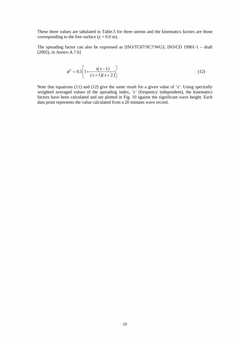
Note that equations (11) and (12) give the same result for a given value of ‘s’. Using spectrally weighted averaged values of the spreading index, ‘s’ (frequency independent), the kinematics factors have been calculated and are plotted in Fig. 10 against the significant wave height. Each data point represents the value calculated from a 20 minutes wave record.

10

3. CREST HEIGHT DISTRIBUTION

There has been considerable interest in wave crest elevations in recent years because of the growing concern about loss of ‘air-gap’ on offshore platforms following a number of well­publicised incidents where this has happened. In the WACSIS (Wave Crest Sensor Inter-comparison Study) joint industry project [Forristall et al. (2002)], a comparison of crest elevations of several wave elevation sensors has been made along with the evaluation of number of second order models for the wave crest height using the data collected [Prevosto and Forristall (2002)]. One of these models, due to Prevosto [Prevosto et al.(2000a)], explicitly takes into account the wave energy spectral bandwidth and directional spreading. It was found that this model gave the best fit to wave crest elevations from simulated 2nd-order directionally-spread seas. The model reflects the fact that in deep water the wave crest elevations in directional waves (3-D) can be a greater proportion of wave height than in equivalent 2-D waves. Here we examine, empirically, how the crest elevation distribution differs between the start, peak and end of storms. This is set in the context of measurement accuracy and the variability among the recorded crest heights from the three wave elevations altimeters mounted on the platform.

3.1 WAVE CREST HEIGHT PROBABILITY

We have examined the predictive accuracy of the three most promising 2nd order crest elevations models identified by Prevosto and Forristall (2002) in the WACSIS project: notably those of Kriebel and Dawson (1993), Forristall (2000) and Prevosto et al. (2000a). For the last three of these models we have tried to examine the effects of directional spreading upon the predicted crest elevation during the different phases of storms.

Three of the second-order models that have been proposed for describing the distribution of wave elevations are considered here. They represent different ways of extending the basic linear narrow-band model to account for non-linear effects as described in Appendix-B.

Fig. 7(a) and 7(h) show the variation of significant wave height and the directional spreading width ( σ ) during the storm phases. Here large values indicate much spreading and those approaching zero indicate almost unidirectional waves. Comparing these two figures shows clearly that directional width reduces as HS increases and vice versa with pronounced directional focusing as the peak of a storm approaches.

Further it has been found that the steepness of the highest waves tends to be greater during the earlier part of storms [see Wolfram et al. (2001)]. This trend is also seen in Fig. 11, which shows the significant steepness, S2 ( S = 2π HS / gT 2 ; To2 = 2π mo / m2 ; mo and m2 are spectral2 o2

moments) plotted against HS for all storms. It is clear that as wave height increases so does steepness and that steepness is greater during the rise of a storm than during its decay. Now from second order wave theory one expects that as steepness increases crest elevation should increase for a given wave height, this is reflected in the second order crest elevation models described in the next section.

3.1.1 Crest height measurement variations between monitors

The approach used by Forristall (2000) was adopted for plotting probability distributions of crest elevation. All measured crest heights were normalised with crest heights predicted by the corresponding Rayleigh distribution at the same probability of exceedance. If the waves are

11

linear, then the crests will follow a Rayleigh distribution and the normalised crest height ratio would be unity at any level of probability. Thus any departure from unity represents non-linearity. The crest height ratios obtained from measurements at the three monitors (Marex, NEc and Ww) for storms 95, 121 and 223 are plotted in Fig. 12. It is evident that the measured wave crests are not linear, irrespective of the location of the monitor on the platform, and are higher than wave crests predicted from linear wave theory. These plots are typical, and the same trend is apparent for all the other storms that the authors have analysed. It is also clear from Fig. 12 that there are variations between the crest heights recorded at the three monitors on the platform. These variations arise largely from the different directions of the storms and the effect that the platform jacket has upon the waves. The up-weather monitor will see waves that, apart from a little reflection, are unaffected by the legs of the jacket and any conductors. The down-weather monitors will be more affected, particularly when a monitor is down-weather of the riser bundle. Although all the monitors are of the same type and have been calibrated some variation between them is possible. Other studies of the comparative performance of wave height sensors show noticeable variations [e.g. Presvosto and Forristall (2002), Vartdal et al. (1989)]. In these studies the EMI laser altimeters have been found to perform well.

3.1.2 Crest height probability during storm phases

In order to illustrate the variations in the crest height probability distributions during different phases of the storm (rise, peak and decay), the crest height ratios for one hour taken from each phase of each storm are plotted in Figs. 13, 14 and 15 respectively for storm 95, 121 and 223. These figures also include the crest height ratio obtained using all the data collected for the complete duration of the storm. The results are presented separately for each monitor. Storms 95 and 223 are both clearly uni-modal in direction at their peaks (see Figs. 3 and 5); and for these storms there is a clear difference in crest height distribution between the peak and the other phases of the storm observed at all three monitors. At the peak of these storms there are a much larger number of high crests than during the other phases. However for storm 121, which has two strong directional components at its peak, there is no such clear trend on two of the three monitors and all phases of the storm appear to have similar crest elevation distributions. The differences in distribution shape between the highly directionally focussed peaks in Storms 95 and 223 and the more spread sea conditions, are comparable to those seen between the output from 2D and 3D second-order random simulations undertaken by Prevosto and Forristall (2002). These simulations show two-dimensional waves generally have higher crest height ratios than three-dimensional waves except at low probability levels (below 10-2), where the 3D waves have slightly higher crest height ratios. Unfortunately because of the scatter and small amount of data it is difficult to be confident about any particular trend in the real data at these low probability levels.

3.2 COMPARISON OF CREST MODELS WITH STORM DATA

The crest heights computed from Forristall, Kriebel and Dawson, Prevosto and Rayleigh models have been compared with the measured wave crests for each monitor for storms 95, 121 and 223. The parameters such as significant wave height (HS), Tm01 ( = 2π m / m ), Tm02 and spreadingo 1

index (s) have been calculated for each 20-minute record and then the data for the whole storm combined together. The results are shown in Figs.16 to 18 for all the monitors and for all the storms. It is immediately clear from these figures that the Rayleigh model significantly under predicts the larger crest height in all cases. All the models based on second order theory have a significantly better fit except for the most extreme crest heights.

The authors had expected that the Prevosto model, which takes account of directional spreading, would be able to distinguish between the phases of the storm as the directional spreading altered

12

but this has not been demonstrated. This model assumes a cos2s form of spreading function; unfortunately, some of the more spread seas in the data are bi-directional, which perhaps explains the somewhat erratic behaviour of the Prevosto model for Storm 121 in Fig. 17, where s (and Tm02) has been calculated for each 20 minute record in the storm separately. However when we assume Tm02 and s are constant for the whole storm and set them, somewhat arbitrarily, as Tm02 = Tm01/1.1 and s = 10, the Prevosto model gave results closer to the two other second-order models as can be seen in Fig.19.

The performance of all three models for this storm 121 is presented for two of the monitors in Fig. 20 in a normalized form. All the second order models give good predictions for crest elevation up to around 1.2HS. However for the most extreme crests measured they under predict by around 20 % or so. The authors have checked the original time series and all these extreme data points correspond to valid observations (for example Fig. 21). This is discussed further in section-6.

13

14

4. EXPERIMENTS IN THE WAVE BASIN

The experimental programme has been carried out in the multidirectional wave basin of the Department of Civil & Offshore Engineering, Heriot-Watt University. The wave generators are capable of producing unidirectional regular and random waves and random steep short crested waves up to 0.5 m high. The purpose of the experiments was to reproduce extreme storm waves in the basin to measure the wave kinematics in long and short- crested waves with different spreading indices. The measured wave kinematics were then compared with theoretical wave kinematics using linear and hybrid wave models. The wave loading on a circular cylinder due to long and short-crested waves was also measured to calculate the force ratios.

4.1 DESCRIPTION OF THE BASIN

The dimensions of the wave basin are 12m x 12.4m with a working water depth of 3m and a deep pit of 5m in depth. The basin is equipped with a wave making system of electro-mechanical flap-type wave makers across the width of the tank at one end. At the other end of the tank there is a parabolic mesh beach that effectively dissipates most of the wave energy. There are 24 wave paddles in the wave making system, each paddle is 0.5m wide and is independently controlled so that both long-crested and short-crested waves can be produced. The wave maker can generate regular and random waves in the frequency range of 0.2 – 2.5 Hz. A computer drives the paddles using the ‘Ocean’ software developed and installed by Edinburgh Designs [Rogers and King (1997)].

4.2 EXPERIMENTAL RIG AND WAVE PROBE ARRAY

An experiment rig has been designed and built to support the current meters so that measurements of the particle kinematics can be made below the waves on a horizontal grid at different depths. This horizontal grid can be raised and lowered to make measurements at different heights allowing a 3-D array of point measurements during a series of repeat experiments. The rig is shown in Plate.1.

In essence the rig comprises of two horizontal square frames. The lower frame is fixed to the bottom of the basin; adjustable legs attach the upper frame to it so that the elevation of the upper frame can be adjusted between experimental runs. Five detachable aluminium blocks, each with a central hole for fixing the current meters, are to the top frame, one at the centre of the frame and other four blocks at four corners of the top square frame. The blocks can be moved in the horizontal plane on the upper frame to any desired location to allow a variety of measurement configurations. The current meters are fixed in the holes in an inverted position so that the body of the devices are below the measuring heads and all the connecting cables are far away from the measuring region to ensure that the measurements will be free from disturbances as far as possible. The rig has an overall height of about 2m and is made from mild steel hollow square sections and stainless steel bars with considerable cross bracing to ensure it remains rigid during the experiments.

Another aluminium frame with same plan dimensions as the top frame of the experiment rig has been fabricated, onto which six wave probes [P1, P2, P3, P4, P5&P6] are fixed as shown schematically in Fig.22. Wave probes are placed directly above the current meters to avoid any phase delay between the wave and velocity records.

15

4.3 INSTRUMENTATION

Five NDV Velocimeters [Nortek As (2000)] were used in the experiments to measure the wave particle kinematics. The PC-based NDVLab velocimeter [Plate.2], comprises (i) three acoustic receivers & a transmitter mounted on a rigid 40 cm stem, (ii) an end-bell and (iii) a cable of 20 metres to connect to the PC. An assembled velocimeter has a total length of about 70 cm from the tip of the sensors to the bottom end-bell. The NDV probe is attached by the end-bell to the signal-conditioning module, which is in a waterproof housing that holds the receiver. This is pressure rated to a maximum water depth of 30m with operating temperatures from 0° to 40° C. The ADV has an acoustic frequency of 10 MHz and the measuring velocity ranges are ±0.03, 0.10, 0.30, 1.0, or ±2.5 m/s with an accuracy of ±1%. Sampling rate options are available spanning from 0.1 to 25 Hz. The NDVLab version of the system has all the control and communication electronics implemented on a full size PC card that can be inserted into a desktop computer so that the data may be stored directly to hard disk. The optional analog output channel of each ADV card was used so that data from all the wave height probes and the current meters could be collected on a common time base. Data from the wave probes and current meters was sampled by a Data Translation CIO-DAS6402/16 64-Channel 100 KHz, 16 bit, ADC using LabVIEW 4.1. The water in the basin was seeded with hollow glass spheres (Trade name: Spherical-110P8, manufactured by Potters Industries Inc, Southpoint, USA) to ensure proper functioning of the velocimeters during measurements.

4.4 STORM WAVES REPRODUCTION

Storms 95,121 and 223 were selected for reproduction in the basin using the Ocean wave software [Rogers and King (1997)]. A scale of 1:55 was chosen to satisfy as closely as possible the constraints imposed by the tank depth, clock-frequency and run number to match the full-scale water depth of 130m, plus tide, at North Alwyn; this choice of scale gave a corresponding depth of 159m. For each storm a three-hour wave elevation time history data from the peak of the storm, corresponding to one monitor record, was scaled down in height and frequency. A 5% lead-in and a 10% roll-off was applied at the start and end of each record respectively using a Hanning window to limit starting and stopping transient waves and consequent damage to the wave paddles. Fig. 23 shows a typical comparison of time-frequency contour plots of wave energy, obtained using the Stockwell transform (S-transform) [Stockwell et al. (1996), Linfoot et al.(2001)], for a portion of the measured and target records. It is evident that the wave groups on the measured times series occur at similar locations on the time-frequency plane as those of the target record. A slight difference in the energy contours at lower energy levels is obvious and these may be ignored, when one is interested in extreme waves. The Ocean software package has only the cos-2s form of directional spreading and hence this type of spreading function was applied to the directional waves with spreading indices s = 2, s = 4, s = 8 and s = ∞ . Each of the three-hour storm records was reproduced in the basin with these four spreading indices. Note that the same wave elevation record (and hence the same spectral energy) was used as input for both unidirectional and multidirectional waves.

4.5 WAVE KINEMATICS MEASUREMENTS

The wave kinematics were measured at depths z = 0.20 m, 0.35 m and 0.50 m below still water level, corresponding to depth of 11m, 19.25m and 27.5m respectively at full-scale. The wave particle velocities in three perpendicular (X,Y & Z) directions, Vx,Vy & Vz and the wave elevations from each probe were recorded simultaneously with a sampling frequency of 25 Hz.

16

The objective of measuring particle kinematics was to quantify the kinematics reduction factor for different sea spreading indices and to validate the particle kinematics, as predicted by linear wave theory and the hybrid wave model [Zhang et al., (1996) and Zhang et al.(1999)].

The hybrid wave model has the capability of predicting short distance wave evolution and kinematics in directional seas. It require time series from a minimum of three wave properties as input; one of the inputs should be a wave surface elevation or a pressure measurement record and others can be measured horizontal velocity components. The model includes the effects of the nonlinear interaction among wave components and is correct up to second order wave steepness. The algorithm consists of two parts: (i) decomposition of a wave time series which decouples the nonlinear contributions from the time series so as to effectively separate the free-wave and bound-wave components; (ii) superposition of wave time series to compute the nonlinear contributions to any wave property and then to superpose them on to those computed from free-wave components. The decomposition part produces free-wave amplitudes, phases and wave directions for the range of frequency considered. The interaction of two-wave components is modeled in the hybrid wave model by using both the conventional mode coupling (MCM) solution [Longuet-Higgins and Stewart (1960)] and the phase modulation method (PMM) [Zhang and Melville (1990)]. The PMM is a complementary solution to the divergence of the MCM because the MCM may not converge if the wavelengths of the two interacting wave components are quite different. Unlike linear wave theory and its various empirical and semi-empirical modifications, the hybrid wave model is valid for finite amplitude waves. It satisfies the continuity equation governing wave-induced fluid kinematics up to the free surface, and up to the second-order in wave steepness.

A typical comparison of the prediction by hybrid wave model and measurements for storm 121 is given in Fig. 24, from an arbitrarily chosen part of the time series and only a portion is shown here for clarity. The measured time series at probe location P4 has been used as input to the hybrid wave model and the prediction is made at probe P2, which is located at about 0.85m downstream of probe P4. The predicted waves are inseparable from the measured time series. For the same part of the waves, the measured particle velocity (Vx) in the wave direction and computed velocities using linear and hybrid wave models at a depth of z = - 0.20 m, are shown together in Fig. 25. The existence of a phase difference between the measured and computed kinematics may be linked with the data collection and processing hardware/software within the NDVLab system, even though all the data have been collected simultaneously by the LabView acquisition system.

The comparison shown in Fig. 26(a&b) between the wave basin measurements, linear wave theory and hybrid wave theory at a depth z = -0.20m, illustrates that the peak velocity estimation from linear wave and hybrid wave theory are very close, whereas the measured peak velocities slightly deviate from both the theories. With reference to Fig. 26(a), the average measured positive peak velocities are about 8.1% higher than the linear wave results and 9.2% higher than the hybrid waves results. From Fig. 26(b), measured positive peak velocities are only 1.9% higher than linear wave theory. The maximum standard deviation is observed to be about 14.3% between measurements and linear waves and the same is about 12.5% between measurements and hybrid model. While these results are typical, many other records showed closer agreement with the measurements. The peak velocity ratios between linear and hybrid model shows good correlation for the above two cases with a maximum error of about 2%. The good agreement between linear wave and hybrid wave theories can be expected because at this depth of measurements, the wave nonlinearity is reduced. A similar trend as above is also observed for other two depths of measurements, z = -0.35 and -0.50.

In order to compute an overall measure of the measured and computed peak velocities, a ratio is defined as:

17

* * *Rml = Vm ; Rmh =

Vm ; Rlh =Vl (13)

Vl Vh Vh

where, Vm, Vl and Vh stands for peak velocities from measurements, linear and hybrid wave model respectively. The ‘*’ symbol is used as ‘p’ for positive peaks and ‘n’ for negative peaks. The means ( R ) and standard deviations ( σ ) of these ratios are given in Table.6. Using the * *

measured particle kinematics it is possible to obtain the wave kinematics reduction factor for short-crested seas. The kinematics reduction factor, FS can be calculated using the following expression [Tucker (1998)]:

σ 2 uF = 2 (14)s σ + σ 2

u v

where σ and σ are the root mean square values of horizontal velocities Vx and Vy respectively. u v

In the case of a directional sea these are the velocity components in-line and perpendicular to the mean wave direction.

Since the particle kinematics were measured at three different depths below the still water level, we have examined the effect of varying the depth of measurement on the kinematics reduction factor. The calculations of Fs have been carried out for three storms and are given in Tables 7, 8 and 9. The current meter at probe P3 was excluded from the analysis as the recordings from this particular instrument were frequently corrupted by severe noise. The mean of the depth averaged

4

values ( ∑wp , n is the number of probe) and their standard deviations for each spreading index nn =1

were calculated and are shown in Table.10.

The spreading factor (FS) values in Tables. 7, 8 & 9 computed using the measured velocities in both the horizontal directions indicate that the kinematics reduction factor does not show any significant variation with respect to changes of measurement depth for all four velocity probes and for all three storms. However these values indicate that, particularly when the sea is wide spread (i.e. for smaller spreading index, s), FS could be different with respect to measurement locations in the horizontal plane, as there exists a considerable variation between the four velocity probes. The depth-averaged spreading factor given in Table.10 reveals that FS increases with increased spreading index irrespective of the wave characteristics. Theoretically a constant value of FS = 1.0 is expected for all uni-directional waves ( s =∞ ). In our experiments, values in the range of 0.985-0.992 were obtained. The lower range of FS = 0.985 may indicate the existence of a transverse velocity component (perpendicular to the main wave direction) in the wave basin resulting from transverse standing waves with an anti-node near the point of measurement.

The kinematics reduction factors computed from measurements at North Alwyn platform and those obtained from the wave basin experiments for the three storms are put together for comparison in Fig. 33. This plot show a very good correlation between the reproduced storms and field measurements for the range of spreading indices considered. These results are discussed in more detail in section 6.3.2.

4.6 FORCE MEASUREMENTS ON THE CYLINDER

The test cylinder was made of stainless steel with a diameter of 38mm and a length of about 3.87m. The bottom of the cylinder was mounted on a universal coupling about which the cylinder could pivot. A load cell (Plate.3) capable of operating both in compression and tension up to 60N

18

has been used for the measurements. The load cell was fixed at the top of the cylinder at a distance of 0.485m from still water level to measure the total in-line component of the wave forces on the cylinder. The active side of load cell was connected to the cylinder by a slotted bush arrangement as shown schematically in Fig. 27. The passive side of the load cell was fixed to a rigid mild steel channel, which in turn was fixed rigidly to an access bridge spanning over the wave basin. The load cell was calibrated both in air and in water.

Since the wave kinematics in multi-directional waves have an additional component in comparison with long-crested waves, the force distributions will be different for both these seas. The direction of the resultant force varies with respect to time in multi-directional sea, whereas, this will be constant in long-crested sea. The following parameters representing the force ratios have been computed from the measurements:

3D ⎤ ⎡Fx 3D ⎤

; φFmean =

⎡⎣ F 2D

⎦mean ⎣ ⎦1 10 =σ Fx

3 D ⎡Fx = / (15)

⎤ F1 10 2 D ⎤Fx 2 D x

φFσ σ ⎣ ⎦mean

; φ /

⎣⎡F ⎦1 10 x /

where, σ Fx2 D and σ Fx

3 D are the force standard deviations in long-crested and short-crested waves

F 2Drespectively, and F 3D are the measured wave forces in the mean wave direction in long and x x

short crested waves respectively. The suffixes ‘mean’ and ‘1/10’ are the mean values of the peak measured forces and one-tenth values of the measured forces respectively. These values are listed in Table.11.

The force reduction is observed to be consistent for all the storms, with a trend that greater spreading gives a larger force reduction. The standard deviation and 1/10th values are smaller than the mean values of the force peaks.

19

20

5. STORM WAVES AND FORCE PREDICTIONS

In this section, the hybrid wave model [Zhang et al. (1999)] was used to investigate the spatial variation of wave crest heights and the particle kinematics field within an area occupied by the North Alwyn platform. In particular, the wave surface elevation and wave particle kinematics were predicted at the locations of the four main columns [C1,C2,C3 & C4] (c.f. Fig.1) [C1 (x = 9.3m; y = 9.3m), C2 (x = 5.2m; y = 39.8m), C3 (x = 62.4m; y = 46.13m) & C4 ( x = 66.5m; y = 15.25m)]. For this purpose a 20 minutes wave record from the three wave altimeters at the peak of each storm was used as input for the decomposition part of the directional hybrid wave model and the predictions were made at the locations of the columns. The kinematics were then used to determine the resultant wave forces on the cylinders at different depths. From these calculations the kinematics reduction factors and force reduction ratios were derived. The results are presented below.

A typical comparison of the measured and recovered (predicted) wave time histories at the Marex and North East corner monitors are shown in Fig. 28, for a portion of the 20min record for storm 121. This shows a satisfactory correlation between measurement and prediction as expected if the model decomposition procedure has been successful.

5.1 PREDICTED CREST HEIGHT DISTRIBUTIONS

The probability distributions calculated for the predicted wave crests at locations C1,C2,C3 and C4 for storms 95,121 and 223 respectively shown in Fig. 29. These figures clearly demonstrate the spatial evolution of the wave crests within the area of a platform. The nonlinearity of the wave crests is shown clearly in these figures.

5.2 SECOND ORDER WAVE KINEMATICS AND FORCES

Using the hybrid wave model, the wave kinematics have been calculated at 19 different depths [z = 0.0m, -5m, -10m, -15m, -20m, -25m, -30m, -35m, -40m, -45m, -50m, -60m, -70m, -80m, -90m, -100m, -110m, -120m, -129m] from still water level to the sea bed, for both 2D and 3D waves. The predicted wave kinematics were used to calculate the in-line wave force acting on each column using Morison’s equation. The expression (15) was then used to calculate the force ratios and the values are set out in Table.12. The variation of the force ratios with depth for each column is plotted in Figs.30 to 32 for the three storms considered. In order to get a comparison between the computed storm wave forces with these experiments and also with others available in the literature [Hogedal et al. (1994) and Chaplin et al. (1995)], a KC number close to the one reported in the above references has been chosen. This was achieved by varying the cylinder diameter for each storm in the Morison’s equation while retaining the values of drag and inertia coefficients as 0.7 and 1.6 respectively. The KC number was calculated using the formula

KC = π HS coth( kd ) , where D is the diameter of the cylinder, k is the wave number associated D

with peak period and d is the water depth; the value of KC number computed is around 12.5.

The reduction of wave forces on a structure in 3D waves is a function of proportion between drag and inertia terms and therefore the reduction can also be related to Keulegan-Carpenter (KC) number and Reynolds number. It is clear from Figs.30 to 32, the force ratios near the mean water level are decreased considerably and reach a lowest value than other depths. Close to the sea bed these ratios are about 0.8, 0.6-0.7 and 0.92 for storms 95, 121,and 223 respectively, whereas at

21

the mean sea level these are smaller, tending to a minimum of around 0.4, 0.4 and 0.45 respectively. Hogedal et al. (1994) obtained a similar reduction in wave forces and discussed that the force reduction will be more in drag dominated forces than the inertia dominated forces; and in the case of identical drag to inertia force ratio, the force reduction will be affected by the degree of directional spreading. They reported a reduction of 40-60% in the in-line forces above the mean water level. Below the mean sea level, the force reductions were by 15-25%, 11-15% and 8-10% for σ = 43o, 30o and for North Sea spread waves respectively.

It is to be noted that for storm 121, which has a bi-modal spreading function, a large reduction in the force ratio is observed. The authors are unable to confirm this tendency of force reduction for a bi-model spread, as the wave database doesn’t have a more reliable data set with significant bi-model spreading.

The average force reduction factors calculated for the four columns using the hybrid wave model up to the mean water level are given in the Table 12 with their corresponding standard deviations. The values of the spreading index (s) obtained for these storms are also included in this table. The maximum values of standard deviation obtained between the four columns are 1.8%, 4% and 2.1% for φFσ

, φ and φF1 10 respectively. The depth averaged force ratios (up to msl) obtained Fmean /

from theoretical calculations and from the present experiments are compared with other researchers’ data sets in Fig. 34. Here only the factors φ & φ

/Fσ F1 10 are used. In this figure the

results of Chaplin et al.(1995) correspond to values calculated for total forces at a KC = 12.4; the 43oresults of Hogedal et al.(1994) correspond to spreading widths, σ = 30o ( s = 6.29) and

( s = 2.55), which are for the depth integrated wave forces averaged for experiments with equal directional spreading. As one can see, in general, the present experimental and theoretical force ratios compare well with the Chaplin et al. and Hogedal et al. values, except for storm 121 (s = 1.92) which has a lower value and this may be attributed to the bi-model nature of the spreading function for this particular storm, which has a peak significant wave height larger than the other two storms. Therefore, in order to investigate what would be the force ratio if the spreading were uni-model, another portion of the record from storm 223 (denoted as storm223a, HS = 3.68 m; TP = 11.07 sec; s = 2.24) has been chosen and the results are included in Table 12 (under storm223a) and also in Fig. 34. The force ratio calculated for storm223a is around 0.72, which is closer to the results of Chaplin et al. Another point to note here is that the Hogedal et al. results are derived for the force ratios from the largest 5% of the force peaks and that their results with a North Sea spreading function with σ = 23o – 57o yielded a factor of 0.875 for the inline forces. The force ratios obtained in the present work suggests that it is dependent on the spreading index (s) or spreading width (σ ). The force ratio decreases with increase in wave spreading.

The in-line force reduction based on the force standard deviation values for the wave basin measurements are about 12%, 18% & 28% respectively for s = 8, 4 & 2; and based on the force 1/10th peak values the reductions are about 12%, 21% and 30% respectively. For the field measurements, forces computed with hybrid wave theory, in-line force reduction based on the force standard deviation values are about 14%, 26% & 28% respectively for s = 8.58, 5.13 & 2.24 and based on the force 1/10th peak values the reductions are about 14%, 24% and 33% respectively. Further discussion on the results is made in section 6.4.

22

6. DISCUSSION AND RECOMMENDATIONS

In this report, although we have presented detailed results for only three storms from a sample of 33 subjected to analysis, similar trends have been observed in many of the others. The data have been obtained using EMI laser altimeters that have proved reliable at North Alwyn and have given consistently good results in comparative studies [Forristall (2002) and Vartdal et al. (1989)]. The wave basin experiments again are based on time series reproduced from the same storms but nonetheless represent typical conditions from which general inferences may be drawn.

6.1 VARIATIONS IN CHARACTERISTICS OF DIRECTIONAL WAVES

In general, the directional wave energy spectra of a uni-modal sea indicated that as the storm grows to its peak intensity, the spectral energy increases and energy becomes more concentrated around a single spectral peak, whereas, for a bi-model sea the energy focussing occur at two spectral peaks. Among the thirty-three storms analysed two storms were found to have bi­directional spreading functions during at their peak. Such storms will be less of a problem for fixed structures than those in which all the wave energy is focused on a single direction. However for floating structures, such as FPSOs, that seek to align themselves with the dominant weather direction they may cause significant problems and would merit further research in this context.

The spreading functions for directionally uni-modal storms showed similar temporal trends and Fig. 6 shows the behaviour for a typical uni-modal case and a bi-modal case. For the uni-modal case, at lower spectral energies, the peak spreading function magnitudes are observed to be low with the energy quite spread. As the storm grows the energy becomes concentrated around the mean wave direction and spreading function has a more pronounced and larger peak. For the bi- directional case the focussing is around two directions rather than one, however only two storms were observed to be bi-directional at their peaks and no general inferences are drawn about these in this Report. The focussing behaviour is also observed in the polar plots (Figs. 3 to 5).

Given the variations in directional spreading it might be supposed that there may be significant variation in the normalised forms of the key parameters of wave height, crest elevation and steepness. However it is seen in the plots (Fig. 7) that the normalised wave height and crest elevation remain remarkably steady. This has also been the case for the other storms analysed. The normalised steepness of the tenth highest waves does show some variation, with steeper waves tending to occur during the rising part of the storm and the steepness reducing as the storm decays. Such a trend may be anticipated from physical reasoning and, again, is generally observed in the other storms analysed. The same trend has been observed in the average and significant wave steepness; see for example Fig. 7(e). This is seen more clearly in Figure 11 where significant steepness for the 20-minute periods in the rising part of a storm are clearly higher than for the decaying parts of the storm.

It would appear from the results presented here, and the other storms analysed, that it is not necessary to distinguish between the various phases of a storm when analysing time series data in an omni-directional manner to obtain wave heights and wave crest elevations. Thus when predicting maximum wave height and crest elevations for traditional design purposes all the data may be used. However when considering wave steepness the data associated with the rising periods of storms should be separated from that associated with storm decay. The latter have lower steepness and will bias any analysis where maximum steepness is important. This will be the case when specifying design conditions for wave impact, green-water on deck, longitudinal strength; among other design assessments.

23

Directional width and long-crestedness parameters [Fig.7, subplots (h)-(i)] have similar temporal variation during storms and clearly alter with the directional focusing at the storm peak. In general, as the storm approaches its peak the directional width reduces and after the storm peak it increase again. The general trend is for the waves to become more long-crested as the storm reaches its peak (note that this means the long-crestedness parameter is lower). After the peak there is some tendency for the waves to become less long crested but this is not always pronounced. Thus in multi-directional analyses for estimating water particle kinematics and long­crestedness it is clearly important to use just those periods associated with the peaks of storms if reliable maxima are to be estimated. These will be important when looking at particle kinematics reduction factors for the newer fixed structure design approaches and for looking at risk associated with loss of air-gap.

• All storm data may be analysed together when considering wave heights and wave crest elevations; but only the rising parts of storms should be considered when looking at extreme wave steepness.

• For the assessment of fixed structures the kinematic reduction factors (spreading functions) for the peak of a storm only should be used when considering the loading for fixed structures. For floating structures more extreme conditions may arise in bi-modal storms and no explicit recommendations can be made from the research described in this report.

6.2 CREST HEIGHT STATISTICS AND DISTRIBUTIONS

As noted above there is little variation in the normalised tenth highest crest heights during the various phases of a storm. However this is just one statistic and when the whole distribution is considered, as in Figs. 13 and 15, there are differences between the peak and the other phases of a storm, for storms that are largely uni-modal in frequency and direction. These differences do vary from one storm to the next as is seen when comparing Figures 13, 14 and 15. These differences are of a similar order to those seen between the records from the three wave height monitors during a storm (Fig. 12). So it was considered reasonable to use all the data from the storms when looking at the distribution of normalised crest elevations.

It is clear is that when all the data in a storm are considered together they are modelled well enough for engineering purposes by second order models in the region below the extremes as can be seen in Figures 16 to 20. The Rayleigh distribution (based on the linear model) is seen to have a significantly poorer fit in all cases. The linear model assumes waves of low, and effectively constant, steepness whereas the second order models allow for steepness variation. The fact that the steepness is significant and varies through the storm (and hence the data sets) is a reason why the Rayleigh model provides a poorer fit.

The Kriebel and Dawson model has only one more term than the Rayleigh distribution and that term involves the significant or characteristic steepness calculated from the spectrum. On the evidence here it fits the data as well as the other two second order-models that are more complex. The Forristall model has five more terms than the Rayleigh distribution, but it does work in shallow water as well as in deep water. What is encouraging about this model is that, with the coefficients determined from simulated data, it works quite so well with the real wave data presented here. The Prevosto model, which allows for directional spreading, has not worked better with the 3-D wave data than the others as might have been expected. This may be due, at least in part, to the spreading in the directional spectra here being more complex than the simple cos2s form assumed in this model, and the extent of the variations in the directional spectra over the duration of the storms; as illustrated in Figures 3–6 and 8(a). Any one of these three second order models could be used for practical purposes for wave crest elevations up to around 6 m.

24

However for more severe storms these models do not work well for the few extreme crest elevations above around 1.2HS , as can be seen in Fig. 20.

The fact that all the second-order models significantly under-predict the few most extreme measured crest elevation in each storm is of concern. This is clearly the case for all three monitors in all three storms as seen in Figs. 16 to 19. The corresponding time series have been checked visually and all extreme crest elevations investigated. Having three monitors allows an extreme measured on one to be checked on the other two and Fig. 21 provides one such example. The very large crest at 1000 seconds is seen in the 1st and 2nd monitor traces although it is much less pronounced in the 3rd. If all the monitors had recorded approximately the same elevation it would suggest a long-crested wave, the fact that it only appears on two at the same elevation suggests a more short-crested or (and) transient event. In many cases extreme crests are only seen at one monitor. For example, at around 820 seconds on the 2nd monitor the crest elevation is about 12 metres but only 6 or 7 metres on the other two monitors; suggesting a very local event.

In the WACSIS project the second-order models provided good fits to simulated data that mapped well onto real data. However this was in smaller sea states of HS less than 4.5m and crest heights of no more than around 6m. Here the models also seem to work well for crest heights up to at least 6m and the disparities only occur beyond that. The authors are in no doubt that these extreme observations are valid and think they may be due to the greater steepnesses often seen in very large waves. The greater frequency of observation of these very high crests compared with equally extreme waves may at first seem surprising. Now waves are known to be serially correlated [e.g. Stansell et al. (2002)], but assume just for a moment that crest heights and trough depths are not. Then if an extreme crest occurs once in every 1000 waves and an extreme trough as frequently, the joint occurrence to give an extreme wave height would 1 in a 1 000 000. Clearly these odds will be reduced due to serial correlation, but it does explain why extreme crests will be seen much more frequently than extreme waves. Equally clearly extreme wave crests in large storms merit further study.

• The second order models for wave crest elevation from Forristall, Kriebel and Dawson, and Prevesto all provide much better fits to the data than the Rayleigh distribution and can be used with for crest elevations up to 6m. The may be also be used for more severe storms for crest elevations up to 1.2HS.

• Further study is required of extreme wave crest elevations, above 1.2HS. In this region the second order models consistently under-predict the extremes and should only be used with a significant safety margin.

6.3 WAVE SPREADING AND PARTICLE KINEMATIC REDUCTION FACTORS

6.3.1 Field Measurements

The variety of ways of defining and calculating kinematic reduction factors yields a range of values from the same storm conditions. Factors based on velocity measurements are considered in the next section, here factors based on full-scale measurements of surface elevation are considered. Fig. 9 has plots of FS1 and FS2 for the temporal peaks of the three storms which show significant variation with frequency; yielding the largest values close to the peak frequency. The six different reduction factors, using Tucker’s definitions, for each storm are seen in Table.5 to vary significantly. Tucker (1996) suggests that the factors FS 2 ( peak ) and F ( mean ) should3 S 2

be considered for the UK waters; and for the two uni-modal storms considered here the corresponding values are: FS 2 ( peak ) = 0.93 and F ( mean ) = 0.87 for Storm 95 (s = 5.13);3 S 2

and FS 2 ( peak ) = 0.97 and F ( mean ) = 0.91 for Storm 223 (s = 8.58). For data collected at 3 S 2

North Cormorant, which is less than 50 miles from North Alwyn, Tucker (1996) obtained

25

FS 2 values ranging from 0.87 to 0.96 at the height of severe storms with an average of 0.92. He also reported that FS 2 ( peak ) can be as high as 0.97 for some severe storms and gave typical 3

values for extreme significant wave heights of FS 2 ( peak ) = 0.95 and F ( mean ) = 0.90 at3 S 2

moderate depths; very similar to the North Alwyn values obtained here. When considering the extreme wave loading on a jacket structure, which is likely to occur due to a single large wave at or close to the spectral peak frequency, then FS 2 ( peak ) might seem appropriate. However the 3

ISO draft standard [ISO/TC67/SC7/WG3, ISO/CD 19901-1 – draft (2002), in Annex-A.7.6] and all authors, it appears, other than Tucker use just F ( mean ) or an equivalent formulation. S 2

At North Alwyn for any given significant wave height there is a considerable range of spreading index values that can occur as can be seen in Fig. 8, where s is plotted for every 20 minutes record for the whole duration of ten separate storms. In Fig.10, the corresponding F ( mean ) isS 2

seen vary from 0.707 (the minimum theoretical value) to 0.92 and the median value is seen to rise with HS. This trend has also been observed by Forristall and Ewans (1998) in other data sets. These median values of F ( mean ) would be appropriate for fatigue calculations. On the other S 2

hand, for extreme loading on a fixed platform, where the wave length is large compared to the platform dimensions, storms with highest spreading index s will produce the most severe conditions; and so extreme design condition storms need to be characterised by a spreading index as well as by spectral density.

Wave spreading and particle kinematic reduction factors have been found to vary with latitude and this is reflected in the new ISO draft standard. Forristall and Evans (1998) recommended an overall median value of 0.88 (low-latitude monsoons) and a value of 0.867 (tropical cyclones) for waves over 7.0m for engineering calculations, whereas values for extra-tropical areas are somewhat higher. The draft ISO standard (which quotes Forristall and Ewans (1998)) gives an expression for FS 2 as a function of latitude and for that of North Alwyn it is 0.89, which is very similar to the F ( mean ) values above.S 2

6.3.2 Wave basin measurements and comparisons with theory

The good agreement between the time/frequency plots for the full scale and model scale in Fig. 23 illustrates that storm conditions measured at North Alwyn were reproduced well in the wave basin. The corresponding surface elevations measured in the wave basin were modelled well by both linear theory and Zhang’s second order hybrid model, as seen in Fig. 24, and the predicted horizontal velocity at -0.20m depth using both theories is also quite good, as illustrated in Fig. 25. The comparison shown in Fig. 26(a & b) between the wave basin measurements, linear wave theory and hybrid wave theory at a depth z = -0.20m, illustrates that the peak velocity estimation from linear wave and hybrid wave theory are very close; whereas the measured peak velocities deviate slightly from both the theories by a few percent. This is despite the fact that the nominal accuracy of the instruments is ±1%. However the fit between the theories and the measured data varied and in many cases the agreement was better than seen in these figures. Because of the minimum depth of the measurements necessary to ensure the probes were continuously immersed was -0.20m, the difference between linear and second order theory predictions of wave particle velocity were too small to be detected reliably.

Ideally, kinematic reduction factors should be based on the measurement of the wave particle kinematics and this has been done for the experiments in the wave basin. The kinematic reduction factors computed using the measured velocities (FS as defined in equation 14 ) in Tables 7, 8 & 9 show little variation with depth for all the four velocity probes and for all three storms. The

26

depth-averaged spreading factor presented in Table 10 shows the variation between storms of the same spreading index is between 1 and 2%, and much smaller than the variation with spreading index. Theoretically a value of FS = 1.0 is expected for uni-directional waves ( s =∞ ); however values in the range of 0.985-0.992 were obtained, which gives a measure of the error and bias in the experiments. Some of which may be due to measurement error, some due to slight misalignment in the wave basin and some due to stray currents set up in the basin during the experiments.

Fig. 33 shows the mean of the depth averaged kinematics reduction factors (FS) computed using horizontal velocity estimates obtained from the hybrid second order model with the surface elevation measurements made at North Alwyn platform during the three storms. These show generally very good agreement with those obtained from the corresponding wave basin velocity measurements except at s =1.92. However it must be remembered that the field data for this storm, Storm 121, is bi-modal whereas all the storms in wave basin were given cos-2s spreading function and so differences are to be expected at this point. The capacity of the hybrid second order model to represent the wave surface elevation is shown in Fig. 24. These results show 3-D hybrid second order model is able to predict particle kinematics from surface elevations, measured at different points in the horizontal plane, with sufficient accuracy to compare well with measured values.

All the reduction factors in Tables 7-10 and in Fig. 33 are based directly on the variance of horizontal wave particle velocities; or theoretical estimates of this variance from the surface elevation. It would of course be possible to define a reduction factor in terms of the mean of the peak amplitudes of the velocities, or the average of the tenth highest peaks, or even the highest peaks. The question of which definition of FS is appropriate must be considered in the context of the wave loading that is to be estimated.

6.4 WAVE FORCE MEASUREMENTS AND FORCE REDUCTION

The use of the kinematic reduction factors is usually for the estimation of the reduction in wave forces on the tubular members of jacket structures due to directional wave spreading. Therefore direct measurement of wave forces on a vertical circular cylinder in 3-D and 2-D waves allowing the corresponding force reduction (or force ratio) to be simply calculated should, in principle, provide a good check on this process. However the reduction of wave forces on a structure in 3D waves is not just a function of the degree of wave spreading, but also of the relative magnitude of the drag and inertia terms, and hence the Keulegan-Carpenter (KC) number. So the check is not quite as straightforward as it first appears. The experiments involving the measurement of forces on the whole cylinder in 2-D and 3-D have allowed the force ratio to be calculated on the basis of both the average of tenth highest peak forces and the root mean square force. The corresponding force ratios are quite similar as seen in Fig. 34 and, interestingly, the root mean square based ratios are marginally higher than those based on the average of the tenth highest in two cases. Interesting a KC number of 11.4, Chaplin et al.(1995) obtained a similar result. The experimental results of Chaplin et al. and Hogedal et al.(1994) for the root mean square force ratios are also plotted in Fig. 34 and agree quite well with the experimental results obtained here. Interestingly in Table 11 the ratio of the mean peak forces is higher than the ratio of the mean of the 1/10th

highest. The mean of the 1/10th highest is used as a more surrogate for the maximum peak value. This suggests that there is a bigger percentage reduction in peak loads than in average loads when moving from 2-D to 3-D waves.

The force ratio calculated using the hybrid second order models for the legs of the jacket structure are shown in Figs. 30 to 32. These values are based on the field measurements at the three wave monitors at North Alwyn and are computations based on Morison’s equation. In that sense they are quite separate from wave basin measurements. These theoretical results show a big reduction

27

in force at the surface but little variation in force beyond 20m depth in full scale. It is interesting to note that there is no consistent trend in these figures for relative magnitude of the force ratios, calculated in the three different ways, for all the legs in all the storms. The variation of depth-averaged values with spatial positions of the legs of a jacket is seen in Table 12 to range from around 1% to 5%. The means of the depth averaged theoretical values for all four legs are also seen in Fig. 34. The comparison between the experimental values and those for storms 223 and 223a (s = 8.58 and 2.24 respectively) are very good. The comparison for storm 121 (s = 1.92), which is a bi-model sea, is less good as might be expected. The reason why storm 95 does not compare better is not clear especially as the corresponding kinematics reduction factor compares well with the wave basin results.

In light of the above results from full scale measurements of storm waves, the velocity and force measurements it seems that kinematics reduction factor FS2(mean) estimated from surface elevation records, and FS on depth averaged root mean horizontal wave particle velocities are the most suitable definitions for calculating forces on jacket structures. These two definitions give comparable results. The results presented in Fig. 33 for FS and FS2(mean) are similar to those obtained from equations (11) and (12).

• Particle kinematic reduction factors (wave spreading factors) vary with the spreading index s and for the northern North Sea the following values are appropriate:-Fs =0.78 (s =2); Fs =0.85 (s =4); Fs =0.88 (s =6)and Fs =0.92 (s =8).

• Particle kinematics reduction factors estimated from the surface elevation measurements at North Alwyn and the corresponding force ratios estimated using the hybrid second order model, tie-in quite well with the force ratio measurements made in the wave basin.

28

7. CONCLUSIONS

This study investigated some of the properties of storm waves in the northern North Sea using full-scale data measured at a platform and experiments in a multidirectional wave basin where these storms have been simulated. The salient findings derived from this research work are given below.

1. All storm data may be analysed together when considering wave heights and wave crest elevations; but only the rising parts of storms should be considered when looking at extreme wave steepness.

2. For the assessment of fixed structures the kinematic reduction factors (or wave spreading factors) for the peak of the storm only should be used when considering the loading for fixed structures. For floating structures more extreme conditions may arise in bi­directional and bi-modal storms and no explicit recommendations can be made from the research described in this report. These storms, and the responses of FPSOs to them, merit further research.

3. The second order models for wave crest elevation from Forristall, Kriebel and Dawson, and Prevesto all provide much better fits to the data than the Rayleigh distribution and can be used with for crest elevations up to 6m. They may also be used for more severe storms for crest elevations up to 1.2 times the significant wave height (HS).

4. Further study is required of extreme wave crest elevations, above 1.2 HS. In this region the second order models consistently under-predict the extremes and should only be used with a significant safety margin. The difficulty here is that this requires more data in the extremes than is currently available to undertake a reliable extreme value distribution analysis.

5. Particle kinematic reduction factors vary with the spreading index s and for the northern North Sea the following values are appropriate:- Fs = 0.78 (s = 2); Fs = 0.85 (s = 4); Fs = 0.88 (s = 6)and Fs = 0.92 (s = 8).

6. Particle kinematic reduction factors estimated from the surface elevation measurements at North Alwyn and the corresponding force ratios estimated using the hybrid second order model, tie-in quite well with the force ratio measurements made in the wave basin.

29

30

REFERENCES

Aage, C. 1990. Applicability of 3-D wave loads in offshore design. Environmental Forces on Offshore Structures and their Prediction, London Society for Underwater Technology, Kluwer Academic Publishers, 247-260.

Aage, C., Jorgensen. P., Andersen, L.W., Dahl, C. and Klinting, P. 1989. Wave loads on a cylinder in 2-D and 3-D deep water waves, Proc. of the 8th International. Conference on Offshore Mechanics and Arctic Engineering, The Hague, March 19-23, V-2, 175-181.

API, 1993. Recommended practice for planning, designing and constructing fixed offshore structures – load and resistance factor design, American Petroleum Institute, 225.

Banner, M.L. 1990. Equilibrium spectra of wind waves, J Phys Ocean, 20, 966-984.

Benoit, M. 1992. Practical comparative performance survey of methods used for estimating directional wave spectra from heave-pitch-roll data. Proc. 23rd Int. Conf. on Coastal Eng. (ASCE), Venice (Italy), 62-75.

Benoit, M. and Goasguen, G. 1999. Comparative evaluation of directional wave analysis techniques applied to field measurements. Proc. of the 9th International Offshore and Polar Engineering Conference, Brest, France, May 30-June 4, Vol. III, 87-94.

Benoit, M., Frigaard, P. and Schaffer, H.A 1997. Analysing multidirectional wave spectra: a tentative classification of available methods. Proc. IAHR Seminar on multidirectional waves and their interaction with structures, 27th IAHR Congress, San Francisco (USA), 131-154.

Borgman, L.E. 1969. Directional spectra models for design use, Offshore Technology Conference, Houstan, Texas.

Borgman, L.E. 1977. Directional wave spectra from wave sensors, Ocean Wave Climate, Ed. by Earle.M.D and Malahoff.A, Marine science, 8, 269-300.

Briggs, M.J., Thompson, E.F. and Vincent, C.L. 1995. Wave diffraction around breakwater. Jl. of Waterway, Port, Coastal, and Ocean Engineering, 121, No.1, 23-35.

Brissette, F.P. and Tsanis, I.K. 1994. Estimation of wave directional spectrum from pitch-roll buoy data, Jl. Waterway, Port, Coastal and Ocean Engg., 120, 1, 93-115.

Brodtkorb, P.A., Johannesson, P., Lindgren, G., Rychilk, I., Ryden, J. and Sjo, E. 2000. WAFO – A Matlab toolbox for analysis of random waves and loads, In Proceedings of the 10th

International Offshore and Polar Engineering Conference, Seattle, USA, May 28-June 2, 2000, Vol. III, 343-350.

Chaplin, J.R., Subbiah, K. and Irani, M. 1995. Loading on a vertical cylinder in multidirectional waves, Jl. Offshore Mechanics and Arctic Engineering, 117, 151-158.

Chaplin, J.R., Subbiah, K. and Irani, M. ,1993. Effects of wave directionality on the in-line loading of a vertical cylinder, Proc. of the 3th International Offshore and Polar Engineering Conference, Singapore, Jun 6-11, Vol. III, 116-120.

Donelan, M.A., Hamilton, J. and Hui, W.H. 1985. Directional spectra of wind-gathered waves, Phil. Trans. Roy. Soc. London, Ser.A, 315, 509-562.

31

Forristall, G.Z. 2000. Wave Crest distributions: Observations and second-order Theory. J. Physical Oceanography, 30(8), 1931-1943.

Forristall, G.Z. Barstow, S.F. Krogstad, H.E. Prevosto, M., Taylor, P.H. and Tromans, P. 2002. Wave crest sensor intercomparison study: an overview of WACSIS, Proceedings of the 21st

International Conference on Offshore Mechanics and Arctic Engineering, Oslo, Norway, 23-28 June, OMAE 28438.

Forristall, G.Z. and Ewans, K.C. 1998. Worldwide measurements of directional wave spreading, Jl. of Atmospheric and Oceanic Technology, 15, 440-469.

Haring, R.E. and Heideman, J.C. 1980. Gulf of Mexico rare wave return periods, Jl. Pet. Technology, 265, 35-47.

Hashimoto, N. 1997. Analysis of the directional wave spectrum from filed data, Advances in Coastal and Ocean engineering, Edited by Liu, P.L.F, Cornel University, Vol.3, 103-143.

Hashimoto, N. and Konube. K. 1986. Estimation of directional spectra from the maximum entropy principle, Proc. 5th OMAE Symp., Tokyo, 80-85.

Hasselmann, D.E., Dunkel, M. and Ewing, J.A. 1980. Directional wave spectra observed during JONSWAP 1973, . Jl. Phys. Oceanog.,10,1264-1280.

Hasselmann, K. et al. 1973. Measurements of wind-wave growth and swell decay during the joint North Sea Wave Project (JONSWAP), Deutsche Hydr. Zeit, Reihe A (8o), No.2, 95.

Heideman, J.C. and Weaver, O.T. 1992. Static wave force procedure for platform design, Civil Engg in the Oceans 5, Intl. Conference, November, Texas, 496-517.

Hogedal, M., Skourup, J. and Burcharth, H.F. 1994. Wave forces on a vertical smooth cylinder in directional waves, Proc. of the 4th International Offshore and Polar Engineering Conference, Osaka, Japan, April 10-15, Vol. III, 218-223.

Huang, N.E., Bliven, L.F., Long, S.R. and Tung, C.C. 1986. An analytical model for oceanic whitecap coverage, J. Physical Oceanography, 16, 1597-1604.

IAHR. (1986). List of sea-states parameters. Int. Assoc. for Hydraulic Research.

ISO/TC67/SC7/WG3, ISO/DIS 19901-1 (draft). 2002. Petroleum and natural gas industries- specific requirements for offshore structures-Part 1: Metocean design and operating condition.

Isobe, M., Konda, K. and Horikawa, K. 1984. Extension of MLM for estimating directional wave spectrum, Proc. Symp. On Description and Modelling of Directional Seas., Lyngby (Denmark). June 18-20, paper no. A-6.

Jahns, H.O. and Wheeler, J.D. Long-term wave probabilities based on hindcasting of severe storms, J. Pet. Tech. 1973, 473-486.

Jefferys, E.R. 1987. Directional Seas should be Ergodic. Applied Ocean Research. Vol.9, No.4.

Jonathan, P., Taylor, P.H. and Tromans, P.S. 1994. Storm waves in the northern North Sea, BOSS’94, MIT, Boston, MA, Vol.2, 481-494.

32

Kondo, K. and Koning, J.P.A. de. 1986. Comparison of directional sea measurement by an orbital following buoy and a combination of a wave gauge and a current meter, Proc. of the Fifth Int. Conf. on Offshore Mechanics and Arctic Engineering, Vol. I, 51-58.

Kriebel, D.L. and Dawson, T.H. 1991. Nonlinear effects on wave groups in random seas, J. Offshore Mechanics and Arctic Engineering, 113, 142-147.

Kriebel, D.L. and Dawson, T.H. 1993. Nonlinearity in wave crest statistics. In Proceedings of the Second International Symposium on Ocean Wave Measurement and Analysis, ASCE, New Orleans, 61-75.

Krogstad, H.E. 1988. Maximum likelihood estimation of ocean wave spectra from general arrays of wave gauges. Modelling, Identification and Control, 9, 81-97.

Krogstad, H.E., Barstow, S.F., Haug, O. and Peters, D.J.H. 1997. Directional distributions in wave spectra. Proc. of the Third International Symp. Ocean Wave Measurement and Analysis, Vol. 2, 883-895.

Long, R.B. and Hasselmann, K. 1979. A variational technique for extracting directional spectra from multi component wave data. Jl. Phys. Oceanog., 9, 373-381.

Longuet-Higgins, M.S. 1957. The statistical analysis of a random moving surface, Phil. Trans. Royal Soc. London, A 249, 321-387.

Longuet-Higgins, MS., and Stewart, R.W. 1960. Changes in the form of short gravity waves on long waves and tidal currents, J. Fluid Mech, 8, 565-583.

Longuet-Higgins, M.S., Cartwright, D.E. and Smith, N.D. 1963. Observations of the directional spectrum of sea waves using the motions of a floating buoy, Ocean Wave Spectra, Prentice-Hall, 111-136.

Lygre, A. and Krogstad, H.E. 1986. Maximum entropy estimation of the directional distribution in ocean wave spectra. Jl. Phys. Oceanog., 16, 2052-2060.

Massel, S.R. and Brinkman, R.M. 1998. On the determination of directional wave spectra for practical applications, Applied Ocean Research, No. 20, 357-374.

Miles, M.D. and Funke, E.R. 1987. A Comparison of methods for synthesis of directional seas. Proc. of the 6th Int. Conf. on Offshore Mechanics and Arctic Engineering Symposium, Vol.II, 247-255.

Mitsuyasu, H., Tasai, F., Suhara, T., Mizuno, S., Ohkuso, M., Honda, T. and Rikishi, K. 1975. Observations of the directional spectrum of ocean waves using a cloverleaf buoy, Jl. Phys. Oceanog., Vol.5, No.2, 750-760.

Nortek As. 2000. Nortek Velocimeter- Operations manual, Norway (www.nortek-as.com).

Prevosto, M. 1998. Effect of directional spreading and spectral bandwidth on the nonlinearity of the irregular waves, In Proceedings of the 8th International Offshore and Polar Engineering Conference, Montreal, Canada, May 24-29, Vol. III, 119-123.

Prevosto, M. and Forristall, G.Z. 2002. Statistics of wave crests from models vs. measurements, In Proceedings of the 21st International Conference on Offshore Mechanics and Arctic Engineering, Oslo, Norway, 23-28 June, OMAE 28443.

33

Rogers, D. and King. B.G. 1997. Wave generation using Ocean and Wave. Users Manual Ver. 3.61, Edinburgh Designs Ltd.

Stansell, P., Wolfram, J. and Linfoot, B.T. 2002. Statistics of wave groups measured in the northern North Sea: comparisons between time series and spectral predictions, Applied Ocean Research, 24(2), 91-106.

Stansell, P., Wolfram, J. and Zachary, S. 2003. Horizontal asymmetry and steepness distribution for wind driven ocean waves from severe storms, Applied Ocean Research, (accepted for publication).

Tayfun, M.A. 1980. Narrow-band nonlinear sea waves, J. Geophys Res., 1980, 85,1548-1552.

Taylor, P.H. and Gibbs, R.H. 2002. Wave focussing on deep water- bandwidth, spreading and non-linearity. In 7th International Worksop on Wave Hindcasting and Forecasting, Banff, Alberta, Canada, October 21-25.

Tucker, M.J. 1991. Waves in Ocean Engineering – Measurement, Analysis, Interpretation, Ellis Horwood.

Tucker, M.J. 1996. The wave spreading factor in U.K. waters. Offshore Technology Paper, No.OTO 96025, HMSO, London.

Vartal, L., Krogstad, H.E. and Barstow S.F. 1989. Measurements of wave properties in extreme seas during the WADIC experiment. In Proceedings of the 21st Annual Offshore Technology Conference, OTC 5964, 73-82.

Wolfram, J., Feld, G. and Allen, J. 1994. A new approach to estimating extreme environmental loading using joint probabilities, In proceedings of the 7th International conference on the Behaviour of Offshore Structures, 2, 701-714.

Wolfram, J., Linfoot, B.T. and Venugopal, V. 2001a. Evolution of wave characteristics due to storms in North Sea, In International Conference in Ocean Engineering, Indian Institute of Technology, Madras, India, December 11-14, 109-114.

Wolfram, J., Linfoot, B. and Venugopal.V. 2001b. Some results from the analysis of Metocean data collected during storms in the northern North Sea, Journal of the Society for Underwater Technology, Vol.24, No.4, 153-163.

Zhang, J., Melville, W.K., 1990. Evolution of weakly nonlinear short waves riding on long gravity waves. J. Fluid Mech, 214, 321-583.

Zhang, J., Chen, L., Ye, M. and Randall, R.E. 1996. Hybrid wave model for unidirectional irreular waves- part I. Theory and numerical scheme, Applied Ocean Research, 18, 77-92.

Zhang, J., Yang, J., Wen, J., Prislin, I. and Hong, K. 1999. Deterministic wave model for short-crested ocean waves: Part I. Theory and numerical scheme, Applied Ocean Research, 21, pp. 167­188.

34

Table 1 Measurement Devices

MEASUREMENT SENSOR TYPE

1. Wave height H Thorn EMI infra-red laser wave height meter #1 (Marex monitor)

2. Wave height H Thorn EMI infra-red laser wave height meter #2 (Walkway monitor) 3. Wave height H Thorn EMI infra-red laser wave height meter #3

(North East corner monitor) Pressure Pressure transducer

Wind speed U Munro IM 146 anemometer Wind direction θ " " " " "

Current C Valeport electromagnetic current meter Wave particle kinematics " " " " "

Table 2 Statistics calculated in real time

RAW MEASUREMENT STATISTICS Location

Wave height (3 channels) H Significant wave height Hm0

34.33, 30.3 and 24.69 metres

above platform datum

Sea water flow speed C and Mean current vector w.r.t 16 metres below direction φ Magnetic North MWL

Wind speed U and direction θ Mean wind vector w.r.t True North

102 metres above MWL

Table 3 Threshold for Statistics

RAW MEASUREMENT STATISTIC THRESHOLD

Wave height (4 channels) Significant wave height 3.5 m

Wind speed and direction Mean wind vector w.r.t True 16 m/s North

35

36

Table 4 Storm details

Storm Start date & time End date & time Max Hs No. [dd/mm/yy & hr:min] [dd/mm/yy & hr:min] (m)

95 26/09/96 12:58 27/09/96 12:24 7.1

121 06/02/97 06:11 10/02/97 02:51 8.6

223 23/12/99 15:46 26/12/99 10:10 7.2

Table 5 Wave kinematics factors computed based on the definitions by Tucker (1996)

Storm No.

1 1SF ( peak ) 1 3SF ( peak ) S1F ( mean ) 2 1SF ( peak ) 2 3SF ( peak ) S 2F ( mean )

95 0.8714 0.8871 0.8087 0.9127 0.9265 0.8662

121 0.8535 0.8441 0.6619 0.8933 0.8983 0.7838

223 0.9745 0.9662 0.8692 0.9747 0.9653 0.9120

37

Table 6 Comparison of peak velocities from measurements and theories: mean and standard deviations

Cases p mlR p

mhR p lhR n

mlR n mhR n

lhR p mlσ p

mhσ p lhσ n

mlσ n mhσ n

lhσ

Part 1 1.0814 1.0921 1.0126 0.9194 0.9371 1.0201 0.1436 0.1258 0.0443 0.0843 0.1108 0.0770

Part 2 1.0192 1.0007 0.9815 0.9818 0.9691 0.9861 0.1068 0.1133 0.0297 0.0986 0.1209 0.0447

Table 7 Kinematics reduction factor (Fs) for storm 95 calculated from wave basin measurements

Depth of measurements

s = 2 s = 4 s = 8 s = ∞

wp1 wp2 wp4 wp5 wp1 wp2 wp4 wp5 wp1 wp2 wp4 wp5 wp1 wp2 wp4 wp5

-0.20 m 0.719 0.738 0.769 0.764 0.829 0.819 0.794 0.866 0.914 0.901 0.904 0.911 0.991 0.989 0.989 0.993

-0.35m 0.706 0.739 0.762 0.766 0.816 0.835 0.852 0.860 0.924 0.907 0.906 0.916 0.989 0.989 0.984 0.989

-0.50m 0.712 0.718 0.773 0.751 0.811 0.800 0.819 0.834 0.917 0.891 0.901 0.903 0.973 0.987 0.977 0.977

mean (depth averaged 0.712 0.732 0.768 0.760 0.819 0.818 0.822 0.853 0.918 0.900 0.904 0.910 0.984 0.988 0.983 0.986

values) std deviation 0.0065 0.0118 0.0056 0.0081 0.0093 0.0175 0.0291 0.0170 0.0051 0.0081 0.0025 0.0066 0.0099 0.0012 0.0060 0.0083

38

Table 8 Kinematics reduction factor (Fs) for Storm 121 calculated from wave basin measurements

Depth of measurements

s = 2 s = 4 s = 8 s = ∞

wp1 wp2 wp4 wp5 wp1 wp2 wp4 wp5 wp1 wp2 wp4 wp5 Wp1 wp2 wp4 wp5

-0.20 m 0.726 0.761 0.766 0.759 0.831 0.856 0.866 0.861 0.929 0.914 0.911 0.921 0.992 0.990 0.989 0.993

-0.35m 0.723 0.773 0.774 0.764 0.840 0.855 0.866 0.872 0.933 0.924 0.918 0.929 0.995 0.993 0.991 0.995

-0.50m 0.714 0.758 0.779 0.763 0.825 0.850 0.858 0.850 0.925 0.911 0.909 0.916 0.991 0.988 0.987 0.993

mean (depth averaged 0.721 0.764 0.773 0.762 0.832 0.854 0.863 0.861 0.929 0.916 0.913 0.922 0.993 0.991 0.989 0.994

values) std deviation 0.0062 0.0079 0.0066 0.0026 0.0075 0.0032 0.0046 0.011 0.0040 0.0068 0.0047 0.0066 0.0021 0.0025 0.0020 0.0012

Table 9 Kinematics reduction factor (Fs) for Storm 223 calculated from wave basin measurements

Depth of measurements

s = 2 s = 4 s = 8 s = ∞

wp1 wp2 wp4 wp5 wp1 wp2 wp4 wp5 wp1 wp2 wp4 wp5 wp1 wp2 wp4 wp5

-0.20 m 0.735 0.746 0.753 0.737 0.840 0.845 0.865 0.859 0.921 0.905 0.908 0.911 0.992 0.989 0.988 0.993

-0.35m 0.731 0.752 0.756 0.747 0.844 0.851 0.861 0.865 0.928 0.918 0.915 0.923 0.988 0.988 0.984 0.990

-0.50m 0.717 0.735 0.747 0.732 0.826 0.835 0.857 0.843 0.915 0.898 0.900 0.902 0.990 0.988 0.988 0.993

Mean (depth averaged 0.728 0.744 0.752 0.739 0.837 0.844 0.861 0.856 0.921 0.907 0.908 0.912 0.990 0.988 0.987 0.992

values) std deviation 0.0095 0.0086 0.0046 0.0076 0.0095 0.0081 0.0040 0.0114 0.0065 0.0101 0.0075 0.0105 0.0020 0.0006 0.0023 0.0017

39

Table 10 Kinematics reduction factors calculated for wave basin measurements; mean of the depth averaged values and standard deviation values in brackets

Spreading index (s)

Storm 95 Storm 121 Storm 223

2 4 8 ∞

0.743 (0.026) 0.828 (0.017) 0.908 (0.008) 0.985 (0.003)

0.755 (0.023) 0.853 (0.014) 0.920 (0.007) 0.992 (0.002)

0.741 (0.010) 0.849 (0.011) 0.912 (0.006) 0.989 (0.002)

Table 11 In-line force ratios calculated for wave basin measurements

Spreading Storm 95 Storm 121 Storm 223

index (s) Fσ

φ mean

φF 1 10 / φF Fσ

φ mean

φF 1 10 / φF Fσ

φ mean

φF 1 10 / φF

2 0.6787 0.7249 0.6886 0.7181 0.7520 0.6767 0.7517 0.8205 0.7327

4 0.8291 0.8987 0.7964 0.7962 0.8426 0.7649 0.8124 0.8680 0.7993

8 0.8842 0.9552 0.8889 0.8723 0.9400 0.8698 0.8621 0.9441 0.8785

40

Table 12 Depth averaged values of inline force ratios computed from hybrid wave model predictions

Location Storm 95 (s = 5.12) Storm 121 (s = 1.92) Storm 223 (s = 8.58) Storm 223a (s = 2.24)

Fσ φ

mean φF 1 10 /

φF Fσ φ

mean φF 1 10 /

φF Fσ φ

mean φF 1 10 /

φF Fσ φ

mean φF 1 10 /

φF

C1 0.7528 0.7691 0.7544 0.6429 0.6457 0.6236 0.8371 0.8843 0.8391 0.7155 0.7245 0.7214 C2 0.7292 0.8406 0.7582 0.6338 0.6206 0.5751 0.8710 0.9005 0.8505 0.7022 0.6971 0.7352 C3 0.7286 0.7476 0.7403 0.6385 0.6392 0.5843 0.8744 0.8711 0.8792 0.7257 0.7001 0.7071 C4 0.7503 0.7731 0.7743 0.6492 0.6657 0.5934 0.8472 0.8860 0.8428 0.7242 0.7258 0.7122

Mean 0.7402 0.7826 0.7568 0.6411 0.6428 0.5941 0.8574 0.8855 0.8529 0.7169 0.7119 0.7190 (0.0131) (0.0403) (0.0140) (0.0066) (0.0186) (0.0210) (0.0182) (0.0120) (0.0182) (0.0108) (0.0154) (0.0123)

Walkway

51 m

50 m

72.5 m

2 3

C2

C1

C3

C4

30. 85 m

57.25 m

1 KEY Extent of jacket Wave height meter Current meter / pressure transducer

Figure 1 Sensor positions on North Alwyn "A"

N

Np

Ep

Marex

NEc

Ww

51 m

m

50 m

°

°

°

72.5

1.5 m 40.3

3.31.7

Note : Exaggerated for clarity. Np and Ep are platform north and platform east.

Figure 2 The angles between the three monitors

41

(c) 27/09/96 - 13:38 Level curves at:

(a) 26/09/96 - 15:58 Level curves at: 90

30

210

60

240

120

300

150

330

180 0

0.05

0.1

0.15 2.521 5.041 7.56210.08 12.6 15.12 17.64 20.17 22.69 25.21

270

(b) 27/09/96 - 01:58 Level curves at: 90 0.15 16.46

32.9149.3765.8382.2998.74115.2131.7148.1 164.6

180

30

210

60

240

120

300

150

330

0.05

0.1

0

270

90 0.15 1.5813.1614.7426.3237.9039.48411.06 12.65 14.23 15.81

180

30

210

60

240

120

300

150

330

0.05

0.1

0

270

Figure 3 Directional spectra for storm 95: (a) start of the storm, (b) peak of the storm and (c) end of the storm

42

(a) 06/02/97 - 12:51 Level curves at: 90 0.2

30

210

60

240

120

300

150

330

180 0

13 0.05

0.1

0.15

1.3 2.6 3.9 5.199 6.499 7.799 9.099 10.4 11.7

270

(b) 08/02/97 - 03:11 Level curves at: 90

30

210

60

240

120

300

150

330

180 0

0.05

0.1

0.15 5.71611.43 17.15 22.86 28.58 34.3 40.01 45.73 51.44 57.16

270

(c) 10/02/97 - 07:51 Level curves at: 90

30

210

60

240

120

300

150

330

180 0

0.05

0.1

0.15

0.2 1.398 2.796 4.194 5.592 6.99 8.388 9.786 11.18 12.58 13.98

270

Figure 4 Directional spectra for storm 121 : (a) start of the storm, (b) peak of the storm and (c) end of the storm

43

(c) 26/12/99 - 09:06

(a) 23/12/99 - 18:06 Level curves at: 90

30

210

60

240

120

300

150

330

180 0

0.05

0.1

0.15

0.2 1.064 2.128 3.192 4.256 5.319 6.383 7.447 8.511 9.57510.64

270

(b) 24/12/99 - 14:06 Level curves at: 90 0.15 16.18

32.3648.5364.7180.8997.07113.2129.4145.6 161.8

180

30

210

60

240

120

300

150

330

0.05

0.1

0

270

Level curves at: 90 0.2 0.5485 1.0971.6452.1942.7423.2913.8394.3874.936 5.484

180

30

210

60

240

120

300

150

330

0.05

0.1

0.15

0

270

Figure 5 Directional spectra for storm 223 : (a) start of the storm, (b) peak of the storm and (c) end of the storm

44

←

←

←

←

←

←

←

-----------1hr

-----------4hr

-----------8hr

-----------12hr

-----------16hr

-----------20hr

-----------23hr

80100

90 70

80 60

00

←

←

←

←

←

←

←

←←

←-----------1hr

-----------10hr

-----------20hr

-----------30hr

-----------40hr

-----------50hr

-----------60hr

-----------70hr -----------80hr

-----------90hr

0 0.05 0.1 0.15 0.2 0.25 0.3 0.35 0.4 0 0.05 0.1 0.15 0.2 0.25 0.3 0.35 0.4

Frequency (Hz) Frequency (Hz)

2.5 1.4

←

←

←

←

←

←

←

----------1hr

----------4hr

----------8hr

----------12hr

----------16hr

----------20hr

----------23hr →

←

←

←

→

→

→

→

←

→

1hr----------

----------10hr

----------20hr

----------30hr

40hr----------

50hr----------

60hr----------

70hr----------

----------80hr

90hr----------

Spe

ctra

l den

sity

(m2 -s

ec)

Spe

ctra

l den

sity

(m2 -s

ec)

70

50 60

4050

40 30

30 20

20

10 10

1.2

2

Spr

eadi

ng fu

nctio

n,D

( θ)

1

1.5 0.8

0.6 1

0.4

0.5 0.2

0 0

45 90 135 180 225 270 315 360 0 0

45 90 135 180 225 270 315 360

Wave directions (deg) Wave directions (deg)

(a) (b)

Figure 6 Energy spectrum (top) and spreading function (bottom): (a) storm 95 and (b) storm 121

45

Spr

eadi

ng fu

nctio

n,D

( θ)

Wav

e he

ight

par

amet

ers

Cre

st h

eigh

t par

amet

ers

Wav

e pa

ram

eter

s

1.00

0.80

0.60

0.40

0.20

0.00

Time

1.40

1.20

23/1

2/99

23/1

2/99

1.80

1.60

1.40

1.20

1.00

0.80

0.60

0.40

0.20

0.00

Time

2.00

26/1

2/99

26/1

2/99

Cn Cp Cm

(b)

26/1

2/99

00:0

000

:00

00:0

0

26/1

2/99

26/1

2/99

26/1

2/99

12:0

012

:00

12:0

0

Hn

(c) Hp Hm

23/1

2/99

12:0

012

:00

10.00

9.00

8.00

7.00

6.00

5.00

4.00

3.00

2.00

1.00

0.00

Time

Figure 7 Directional wave parameters : storm 223

46

(a)

(sec)Tz

Hs(m)12

:00

24/1

2/99

00:0

0

24/1

2/99

12:0

0

25/1

2/99

00:0

0

24/1

2/99

24/1

2/99

00:0

000

:00

24/1

2/99

24/1

2/99

12:0

012

:00

25/1

2/99

25/1

2/99

00:0

000

:00

25/1

2/99

25/1

2/99

25/1

2/99

12:0

012

:00

12:0

0

27/1

2/99

27/1

2/99

27/1

2/99

00:0

0 00

:00

00:0

0

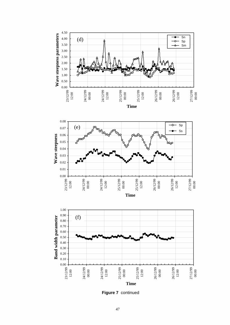
Ban

d w

idth

par

amet

erW

ave

stee

pnes

s W

ave

stee

pnes

s par

amet

ers

0.90

0.80

0.70

0.60

0.50

0.40

0.30

0.20

0.10

0.00

Time

1.00

23/1

2/99

23/1

2/99

0.07

0.06

0.05

0.04

0.03

0.02

0.01

0.00

(e) Sp

Ss

Time

0.08

4.50

4.00

3.50

3.00

2.50

2.00

1.50

1.00

0.50

0.00

23/1

2/99

(f)

12:0

012

:00

12:0

0

Sn Sp Sm

(d)

Time

Figure 7 continued

47

24/1

2/99

00:0

0

24/1

2/99

12:0

0

25/1

2/99

00:0

0

25/1

2/99

24/1

2/99

24/1

2/99

00:0

000

:00

24/1

2/99

24/1

2/99

12:0

012

:00

25/1

2/99

25/1

2/99

00:0

000

:00

25/1

2/99

12:0

012

:00

25/1

2/99

12:0

0

26/1

2/99

26/1

2/99

26/1

2/99

00:0

000

:00

00:0

0

26/1

2/99

26/1

2/99

26/1

2/99

12:0

012

:00

12:0

0

27/1

2/99

27/1

2/99

27/1

2/99

00:0

0 00

:00

00:0

0

Time

Figure 7 continued

48

Lon

g cr

estn

ess p

aram

eter

D

irec

tiona

l wid

th (d

eg)

Mea

n w

ave

dire

ctio

n (d

eg)

0.90

0.80

0.70

0.60

0.50

0.40

0.30

0.20

0.10

0.00

Time

1.00

23/1

2/99

80

70

60

50

40

30

20

10

0

23/1

2/99

Time

90

360

315

270

225

180

135

90

45

0

(g)

23/1

2/99

12:0

0

(h)

σ θκ

12:0

012

:00

24/1

2/99

00:0

0

(i)

00:0

024

/12/

9924

/12/

9900

:00

00:0

0

24/1

2/99

24/1

2/99

24/1

2/99

12:0

012

:00

12:0

0

25/1

2/99

25/1

2/99

25/1

2/99

00:0

000

:00

25/1

2/99

12:0

0

25/1

2/99

12:0

025

/12/

9912

:00

26/1

2/99

26/1

2/99

26/1

2/99

00:0

000

:00

00:0

0

26/1

2/99

26/1

2/99

26/1

2/99

12:0

012

:00

12:0

0

27/1

2/99

27/1

2/99

27/1

2/99

00:0

0 00

:00

00:0

0

49

(a)

(b)

Figure 8 (a) Relationship between Fourier coefficients, r1& r2 and

(b) Significant wave height Vs spreading index (s)

0 0.2 0.4 0.6 0.8 10

0.1

0.2

0.3

0.4

0.5

0.6

0.7

0.8

0.9

1

←-------- Cos-2s

Poisson ---------→

r1

sqrt(

r2)

2 3 4 5 6 7 8 9 101

2

3

4

5

6

7

8

9

10

11

Hs(m)

Spr

eadi

ng in

dex

(s)

0 0.05 0.1 0.15 0.2 0.25 0.3

10-3

10-2

10-1

100

101

102

103

2

Sηη

Fs1 Fs2

Spe

ctra

l den

sity

(m /

Hz)

0.55

0.6

0.65

0.7

0.75

0.8

0.85

0.9

0.95

Wav

e ki

nem

atic

s fa

ctor

0 0.05 0.1 0.15 0.2 0.25 0.3 Frequency (Hz)

0 0.05 0.1 0.15 0.2 0.25 0.3

10-3

10-2

10-1

100

101

102

103

2

Sηη

Fs1 Fs2

1

Spe

ctra

l den

sity

(m /

Hz)

0.6

0.65

0.7

0.75

0.8

0.85

0.9

0.95

Wav

e ki

nem

atic

s fa

ctor

0 0.05 0.1 0.15 0.2 0.25 0.3 Frequency (Hz)

0 0.05 0.1 0.15 0.2 0.25 0.3

10-3

10-2

10-1

100

101

102

103

2

Sηη

Fs1 Fs2

1

Spe

ctra

l den

sity

(m /

Hz)

0.3

0.4

0.5

0.6

0.7

0.8

0.9

Wav

e ki

nem

atic

s fa

ctor

0 0.05 0.1 0.15 0.2 0.25 0.3 Frequency (Hz)

Figure 9 Wave spreading factors with frequency; storm 95 (top), storm 121(middle) and storm 223(bottom)

50

51

Figure 10 Significant wave height Vs spreading factor (φ )

2 3 4 5 6 7 8 9 100.7

0.75

0.8

0.85

0.9

0.95

Hs(m)

Spr

eadi

ng fa

ctor

52

Figure 11 Wave steepness against significant wave height for three storms 95,121 and 223: Top-Marex; Middle-Walkway; bottom-North East corner monitors. Filled circles represent wave conditions before the peak of the storm and empty circles

represent wave conditions at the peak and during decay of the storms

2 3 4 5 6 7 8 90.035

0.04

0.045

0.05

0.055

0.06

0.065

0.07

0.075

0.08

Hs

Ste

epne

ss, S

2

Marex

2 3 4 5 6 7 8 90.03

0.04

0.05

0.06

0.07

0.08

0.09

Hs

Ste

epne

ss, S

2

Ww

2 3 4 5 6 7 8 90.03

0.04

0.05

0.06

0.07

0.08

0.09

Hs

Ste

epne

ss, S

2

NEc

53

10-310-210-11000.8

0.9

1

1.1

1.2

1.3

Probability of Exceedance

Cre

st H

eigh

t / R

ayle

igh

Storm95

MarexWwNEc

10-310-210-11000.8

0.9

1

1.1

1.2

1.3

Probability of Exceedance

Cre

st H

eigh

t / R

ayle

igh

Storm121

MarexWwNEc

10-310-210-11000.8

0.9

1

1.1

1.2

1.3

Probability of Exceedance

Cre

st H

eigh

t / R

ayle

igh

Storm223

MarexWwNEc

Figure 12 Comparison of crest height ratio between monitors

54

10-310-210-11000.8

0.9

1

1.1

1.2

1.3

Probability of Exceedance

Cre

st H

eigh

t / R

ayle

igh

Storm95-Marex

StartPeakEndAll data

10-310-210-11000.8

0.9

1

1.1

1.2

1.3

Probability of Exceedance

Cre

st H

eigh

t / R

ayle

igh

Storm95-Ww

StartPeakEndAll data

10-310-210-11000.8

0.9

1

1.1

1.2

1.3

Probability of Exceedance

Cre

st H

eigh

t / R

ayle

igh

Storm95-NEc

StartPeakEndAll data

Figure 13 Crest height ratios during storm phases for storm 95

55

10-310-210-11000.8

0.9

1

1.1

1.2

1.3

Probability of Exceedance

Cre

st H

eigh

t / R

ayle

igh

Storm121-Ww

StartPeakEndAll data

10-310-210-11000.8

0.9

1

1.1

1.2

1.3

Probability of Exceedance

Cre

st H

eigh

t / R

ayle

igh

Storm121-NEc

StartPeakEndAll data

10-310-210-11000.8

0.9

1

1.1

1.2

1.3

Probability of Exceedance

Cre

st H

eigh

t / R

ayle

igh

Storm121-Marex

StartPeakEndAll data

Figure 14 Crest height ratios during storm phases for storm 121

56

10-310-210-11000.8

0.9

1

1.1

1.2

1.3

Probability of Exceedance

Cre

st H

eigh

t / R

ayle

igh

Storm223-Marex

StartPeakEndAll data

10-310-210-11000.8

0.9

1

1.1

1.2

1.3

Probability of Exceedance

Cre

st H

eigh

t / R

ayle

igh

Storm223-NEc

StartPeakEndAll data

10-310-210-11000.8

0.9

1

1.1

1.2

1.3

Probability of Exceedance

Cre

st H

eigh

t / R

ayle

igh

Storm223-Ww

StartPeakEndAll data

Figure 15 Crest height ratios during storm phases for storm 223

57

1001011021030

1

2

3

4

5

6

7

Number of Exceedances

Cre

st H

eigh

t(m)

Storm95-Marex

dataForristallPrevostoKriebelRayleigh

1001011021030

1

2

3

4

5

6

7

Number of Exceedances

Cre

st H

eigh

t(m)

Storm95-Ww

dataForristallPrevostoKriebelRayleigh

1001011021030

1

2

3

4

5

6

7

8

Number of Exceedances

Storm95-NEc

Cre

st H

eigh

t(m)

dataForristallPrevostoKriebelRayleigh

Figure 16 Crest probability distribution for storm 95: comparison of measured crest heights with models

58

1001011021031040

1

2

3

4

5

6

7

8

9

Number of Exceedances

Cre

st H

eigh

t(m)

Storm121-Marex

dataForristallPrevostoKriebelRayleigh

1001011021031040

2

4

6

8

10

12

Number of Exceedances

Cre

st H

eigh

t(m)

Storm121-Ww

dataForristallPrevostoKriebelRayleigh

1001011021031040

1

2

3

4

5

6

7

8

9

Number of Exceedances

Storm121-NEc

Cre

st H

eigh

t(m)

dataForristallPrevostoKriebelRayleigh

Figure 17 Crest probability distribution for storm 121: comparison of measured crest heights with models

59

1001011021031040

1

2

3

4

5

6

7

8

9

Number of Exceedances

Cre

st H

eigh

t(m)

Storm223-Marex

dataForristallPrevostoKriebelRayleigh

1001011021031040

2

4

6

8

10

12

Number of Exceedances

Cre

st H

eigh

t(m)

Storm223-Ww

dataForristallPrevostoKriebelRayleigh

1001011021031040

2

4

6

8

10

Number of Exceedances

Storm223-NEc

Cre

st H

eigh

t(m)

dataForristallPrevostoKriebelRayleigh

Figure 18 Crest probability distribution for storm 223: comparison of measured crest heights with models

60

1001011021031041050

1

2

3

4

5

6

7

8

9

Number of Exceedances

Cre

st H

eigh

t(m)

Storm121-Marex

dataForristallPrevostoKriebelRayleigh

1001011021031041050

2

4

6

8

10

12

Number of Exceedances

Cre

st H

eigh

t(m)

Storm121-Ww

dataForristallPrevostoKriebelRayleigh

1001011021031041050

1

2

3

4

5

6

7

8

9

Number of Exceedances

Storm121-NEc

Cre

st H

eigh

t(m)

dataForristallPrevostoKriebelRayleigh

Figure 19 Crest probability distribution for storm 121: Prevosto model recomputed with Tm02 = Tm01/1.1 and s = 10

61

0 0.2 0.4 0.6 0.8 1 1.2 1.40

0.2

0.4

0.6

0.8

1

1.2

1.4

Mea

sure

d C

rest

/Mod

el c

rest

Storm121-Marex

Forristall

0 0.2 0.4 0.6 0.8 1 1.2 1.40

0.2

0.4

0.6

0.8

1

1.2

1.4

Prevosto

0 0.2 0.4 0.6 0.8 1 1.2 1.40

0.2

0.4

0.6

0.8

1

1.2

1.4

Measured Crest Height/Hs

Kriebel

0 0.2 0.4 0.6 0.8 1 1.2 1.40

0.2

0.4

0.6

0.8

1

1.2

1.4

Rayleigh

0 0.2 0.4 0.6 0.8 1 1.2 1.40

0.2

0.4

0.6

0.8

1

1.2

1.4

Mea

sure

d C

rest

/Mod

el c

rest

Storm121-Ww

Forristall

0 0.2 0.4 0.6 0.8 1 1.2 1.40

0.2

0.4

0.6

0.8

1

1.2

1.4

Prevosto

0 0.2 0.4 0.6 0.8 1 1.2 1.40

0.2

0.4

0.6

0.8

1

1.2

1.4

Measured Crest Height/Hs

Kriebel

0 0.2 0.4 0.6 0.8 1 1.2 1.40

0.20.40.60.8

11.21.41.6

Rayleigh

Figure 20 Predictive accuracy of crest height models for storm 121: Marex (upper)

Walkway (lower). Prevosto model computed with Tm02 = Tm01/1.1 and s = 10

)W

ave

surfa

ce e

leva

tion

(m

10

5

0

-5

-10 0 200 400 600 800 1000 1200

15

10

5

0

-5

-10

Marex

10

5

0

-5

-10

0 400 600

Ww

200 800 1000 1200

NEc

0 200 400 600 800 1000 1200 Time (sec)

Figure 21 Time series of a 20-minute wave surface elevation recorded by the three wave height altimeters during storm 223 at North Alwyn platform

62

P5, x = 0.4, y = 0.45

Waves

P3, x = 0.0, y = 0.9 P4, x = 0.0, y = 0.0

x

y

P5, x = 0.4, y = 0.45

Freq

uenc

y (H

z)

Freq

uenc

y (H

z)

P1, x = 0.8, y = 0.9 P6, x = 0.8, y = 0.45 P2, x = 0.8, y = 0.0

Not to scale, coordinates are in meter

Figure 22 Schematics arrangement of square array

Target 1.5

1

0.5 10 20 30 40 50 60 70 80 90 100 110

Time (sec)

Measured 1.5

1

0.510 20 30 40 50 60 70 80 90 100 110

Time (sec)

Figure 23 S-transform plots

63

Plate 1. Current meters mounted onto the experimental rig for wave kinematics measurements

Plate 2. Current meter

64

0

leva

ti(m

) id

-0.08

-0.06

-0.04

-0.02

0.02

0.04

0.06

0.08

0.1

Wav

e E

on

Measured Hybr

85 90 95 100 105

Time(sec)

Figure 24 Wave elevation for Storm 121: measured and predicted

0

il

(m/s

)

id

-0.2

-0.15

-0.1

-0.05

0.05

0.1

0.15

Hor

zont

al V

eoc

ity

Measured HybrLinear

85 90 95 100 105

Time(sec)

Figure 25 Wave elevation for Storm121: measured and predicted

65

0.25 0.25

0.20 0.20 Vx

-Hyb

rid m

odel

(m/s

) Vx

-Hyb

rid m

odel

(m/s

) Vx

-Lin

ear t

heor

y (m

/s) 0.15

0.10

0.05

0.00

-0.05

-0.10

-0.15

Vx-H

ybrid

mod

el (m

/s)

Vx-H

ybrid

mod

el (m

/s)

Vx-L

inea

r the

ory

(m/s

) 0.15

0.10

0.05

0.00

-0.05

-0.10

-0.15

-0.20 -0.20

-0.25 -0.25 -0.25 -0.15 -0.05 0.05 0.15 0.25 -0.25 -0.15 -0.05 0.05 0.15 0.25

Vx-Measured (m/s) Vx-Measured (m/s)

0.25 0.25

0.20 0.20

0.15

0.10

0.05

0.00

-0.05

-0.10

-0.15

0.15

0.10

0.05

0.00

-0.05

-0.10

-0.15

-0.20 -0.20

-0.25 -0.25 -0.25 -0.15 -0.05 0.05 0.15 0.25 -0.25 -0.15 -0.05 0.05 0.15 0.25

Vx-Measured (m/s) Vx-Measured (m/s)

0.25 0.25

0.20 0.20

0.15

0.10

0.05

0.00

-0.05

-0.10

-0.15

0.15

0.10

0.05

0.00

-0.05

-0.10

-0.15

-0.20 -0.20

-0.25 -0.25 -0.25 -0.15 -0.05 0.05 0.15 0.25 -0.25 -0.15 -0.05 0.05 0.15 0.25

Vx-Linear theory (m/s) Vx-Linear theory (m/s)

(a) (b)

Figure 26 Comparison peak velocities (Vx) in the wave basin measurements for storm 121 for two different parts of time series

66

Plate 3. Load cell

Wave direction

Load Cell

+

Channel

Cylinder

Plan view

Figure 27 Schematic diagram of force measurement set-up

67

Storm121; Marex ; Short-crested 8

-6

-4

-2

0

2

4

6 i

)W

ave

elev

aton

(m

Measured Predicted

Wav

e el

evat

ion

(m)

-8 300 350 400 450 500

Time(sec)

Storm121; NEc ; Short-crested 8

6

4

2

0

-2

-4

-6

Measured Predicted

-8 300 350 400 450 500

Time(sec)

Figure 28 Comparison between input and recovered wave elevations using hybrid wave model: (i) Marex (top) and (ii) North-East corner (bottom) monitors

68

Storm95 1.3

1.2

1.1

1

Cre

st H

eigh

t / R

ayle

igh

Cre

st H

eigh

t / R

ayle

igh

Cre

st H

eigh

t / R

ayle

igh

0.9

0.8100

C1 C2 C3 C4

10-1 10-2 10-3

Probability of Exceedance

Storm121 1.3

1.2

1.1

1

0.9

0.8100

C1 C2 C3 C4

10-1 10-2 10-3

Probability of Exceedance

Storm223 1.3

1.2

1.1

1

0.9

0.8100

C1 C2 C3 C4

10-1 10-2 10-3

Probability of Exceedance

Figure 29 Crest probability distributions: Hybrid wave model predictions at C1,C2,C3 & C4 for storms 95,121and 223

69

Dep

th (m

)

Column-C1 Column-C2 0

φFσ φφF1/

Fmean

10

0

-20 -20

-40 -40

φFσ φφF1/

Fmean

10

Dep

th (m

)

-60 -60

-80 -80

-100 -100

-120 -120

0 0.2 0.4 0.6 0.8 1 1.2 0 0.2 0.4 0.6 0.8 1 1.2 Force ratio Force ratio

Column-C3 Column-C4 0

)

φFσφφF1/

0

)

φFσφφF1/-120

-100

-80

-60

-40

-20

Dep

th (m

Fmean

10 -120

-100

-80

-60

-40

-20

Dep

th (m

Fmean

10

0 0.2 0.4 0.6 0.8 1 1.2 0 0.2 0.4 0.6 0.8 1 1.2 Force ratio Force ratio

Figure 30 Force ratio with depth for storm 95

70

Dep

th (m

)

Column-C1 Column-C2 0

φFσ φφF1/

Fmean

10

0

-20 -20

-40 -40

φFσ φφF1/

Fmean

10

Dep

th (m

)

-60 -60

-80 -80

-100 -100

-120 -120

0 0.2 0.4 0.6 0.8 1 1.2 0 0.2 0.4 0.6 0.8 1 1.2 Force ratio Force ratio

Column-C3 Column-C4 0

)

φFσφφF1/

0

)

φFσφφF1/-120

-100

-80

-60

-40

-20

Dep

th (m

Fmean

10 -120

-100

-80

-60

-40

-20

Dep

th (m

Fmean

10

0 0.2 0.4 0.6 0.8 1 1.2 0 0.2 0.4 0.6 0.8 1 1.2 Force ratio Force ratio

Figure 31 Force ratio with depth for storm 121

71

Dep

th (m

)

Column-C1 Column-C2 0

φFσ φφF1/

Fmean

10

0

-20 -20

-40 -40

φFσ φφF1/

Fmean

10

Dep

th (m

)

-60 -60

-80 -80

-100 -100

-120 -120

0 0.2 0.4 0.6 0.8 1 1.2 0 0.2 0.4 0.6 0.8 1 1.2 Force ratio Force ratio

Column-C3 Column-C4 0

)

φFσφφF1/

0

)

φFσφφF1/-120

-100

-80

-60

-40

-20

Dep

th (m

Fmean

10 -120

-100

-80

-60

-40

-20

Dep

th (m

Fmean

10

0 0.2 0.4 0.6 0.8 1 1.2 0 0.2 0.4 0.6 0.8 1 1.2 Force ratio Force ratio

Figure 32 Force ratio with depth for storm 223

72

0.5

0.6

0.7

0.8

0.9

1

Field (F )

Wav

e ki

nem

atic

s fa

ctor

Exp(storm95) Exp(storm121) Exp(storm223)

Smean

0 2 4 6 8 10 Spreading index (s)

Figure 33 Wave kinematics factors computed from field and wave basin measurements

1

0.9

0.8

0.7

0.6

0.5

0.4

(φ ) (φFσ

) (φF1/ )

(φFσ)

(φF1/ ) li l.( )

(

Theory FmeanTheoryTheory 10ExpExp 10Chap n et a 1995Hogedal et al. 1994)

0 2 4 6 8 10 Spreading index (s)

Figure 34 Comparison of in-line force ratios; experiments and theory

Forc

e ra

tio

73

74

APPENDICES

Appendix A: Directional Parameters

The nth spectral moment of the frequency spectrum S( f ) is defined as

mn

∞

∫= nS f ( f )df (A.1) 0

It can be shown that

m0

∞

∫= S( f )df = total energy of the wave system (A.2) 0

Using the spectral moments, several wave parameters such as significant wave height (Hs), mean zero crossing period (Tz) and spectral width ( ν ) etc., can be calculated as follows

4 m (A.3)H =s o

1 / 2)T ( m / (A.4)= m2z o

1 / 2⎛

−⎞⎟⎟⎠

1m m 2o 2m1

⎜⎜⎝

=ν (A.5)

From the Fourier coefficients of directional spreading functions, the following directional parameters can be computed, which are used represent the directional spreading function, are listed below:

(i) Mean wave direction:

⎛⎜⎜

⎞⎟⎟

−1 b1θ (A.6) =tanM a1⎝ ⎠

where a1,b1,a2 and b2 are Fourier coefficients of the spreading function.

Tucker (1991) defined mean wave direction by Eq.(A.7) in which the measured directional spectrum is represented as a vector with magnitude S(f) and direction θM and the these vectors summation results a mean wave direction, MDIR.

⎛⎜⎜

⎞⎟⎟

−tan 1 bMDIR = (A.7)

⎝a ⎠

75

where,

S( f )cos [θ ( f )] df∫ Ma = (A.8)

S( f )df∫

S( f ) sin [θ ( f )] df∫ Mb = (A.9)

S( f )df∫ (ii) Directional width:

1 / 22( a1σ = ( 12 − 2 + b1 )) (A.10)

(iii) Mean spreading angle:

⎜ ⎞⎞ 1 / 2 ⎞

2 2 ⎟⎛ ⎛ 1 b1 ( 1 + a )− ( bba )+ ⎛⎜

1 a1 ( 1 − a2 )⎠⎟⎠⎟⎟ ⎟2 1 1 2

θκ = tan − 1 ⎜⎜ ⎝

⎜⎜ 2 ( a + b1

⎝) 2

(A.11)2 2 ⎟ ⎜ 1 ⎟ ⎜ ⎟⎝ ⎠

(iv) Long-crestedness parameter

2⎛ 1 − a2 + b22

⎟⎞

1 / 2

(A.12)Γ =⎜ ⎜ 2 ⎝ 1 + a2 + b2

2 ⎟⎠

Both Long-crestedness parameter and mean spreading angle will have a zero value for uni­directional waves ( Benoit (1999)).

(v) Significant wave steepness:

2π H S= (A.13)SS gT 2 Z

where, TZ is the mean zero-crossing period.

(vi) Average wave steepness:

2π H S= (A.14)SP gTp 2

where, Tp is the peak period.

76

Appendix B: Crest distribution models

Rayleigh model: If the wave surface elevation is considered to be a narrow-banded Gaussian process then the wave crests are adequately represented by a Rayleigh distribution [Longuet-Higgins (1957)]. The probability of wave crests exceeding a given amplitude for narrow-band sea based on linear wave theory is thus:-

( ⎛ CrP > a) = exp

⎝⎜⎜−

8 Ha

S 2

2

⎠⎟⎞⎟ (B.1)

where, Cr is the crest height, a is the amplitude of the linear wave, Hs ( = 4 m ) is theo

significant wave height and mo is the variance of the wave surface elevation and the zero-moment of the wave energy spectrum (i.e. the area under the spectrum).

Forristall model: This model for wave crest elevation, c, has been developed using the results of second order simulations of the sea surface [Forristall (2000)]. The model is based on a two parameter Weibull distribution, which can be viewed as a generalised form of the Rayleigh distribution. It has terms to account for steepness and, through the Ursell parameter, for depth.

⎧ ⎪⎪ ⎛ c ⎞β ⎫

P( C > c ) = exp ⎨−⎜ ⎟⎜ ⎟ ⎬ (B.2)r ⎪ ⎝ α Hs

2 ⎠ ⎪⎩ ⎭

with α α +α S1 + α U ⎫= 1 2 3 r ⎪

⎬ (B.3)β = β − β S1 − β U + β4U 2 ⎪1 2 3 r r ⎭

where, S is the steepness and U is the Ursell number given respectively by1 r

2π H H = s = s (B.4)Ur 2S1 gT 2 k d 3

01 01

The α and β coefficients have been estimated separately for both 2-dimensional and 3­dimensional sea states from the simulations and the resulting parameters are:

1 ⎫α = . .+ 0 2892 S1 + 0 1060Ur ⎪For 2D fit: 8 ⎬ (B.5) 2 . .β = − 2 1597 S1 + 0 968Ur

2 ⎭⎪

1 ⎫α = . .+ 0 2568 S1 + 0 0800Ur ⎪For 3D fit: 8 ⎬ (B.6) β = −1 7912 S1 − 0 5302U + 0 968U 2 ⎪2 . . r . r ⎭

The test of an empirical model with coefficients determined by a particular set of data is how well it predicts results for other, independent, sets of data. This is seen in the next section.

Kriebel and Dawson model: This model is based on the Stokes type second-order wave theory for narrow-band unidirectional seas where the surface elevation at a point can be expressed as

77

2η ( )=a t t + t t +t ( )cos (ω φ )+1 k a ( )cos 2(ω φ ) (B.7)2

where a t is the modulated amplitude of the linear wave components, φ is the slowly-varying ( )phase, ω = m / m 0 is the mean wave frequency, where m0 and m1 are the spectral moments 1

2and k =ω / g is the wave number for the deep water case in which we are interested here.

The corresponding non-linear crest amplitude is

c a= +1 k a 2 (B.8)2

Rearranging this equation to express a in terms of c and substituting back into equation (B.1) provides a simple second order model for wave crest elevation. Models of this type have been considered by Tayfun (1980), Huang et al.(1986) and Kriebel and Dawson (1991,1993) for both deep and shallow water.

In their transformation of equation (B.8) Kriebel and Dawson considered series approximations rather than the exact solution. Here we consider their deep water model with the exact solution.

2 ⎞ Cr P > c) = exp

⎝⎜⎜⎛−

k H 2 ( + − 1 + 2kc ) ⎟ (B.9)8 1( 2 ⎟S ⎠

This form is the same as that produced by Tayfun for infinite depth. This model has no empirical coefficients but it is based on deep water, narrow-bandwidth uni-directional wave considerations. The last model considered here takes explicit account of the degree of energy spreading in the spectrum.

Prevosto model: The model of Prevosto et al. (2000a) is again based on the non-linear transformation of the Rayleigh probability distribution. From second order irregular wave considerations the non-linear crest elevation Cr is expressed in terms of the linear crest height Clin as:

D S 2C Clin + ⎡T ( fm )+T ( fm )⎦⎤C − T D ( fm )H 8

s 2

(B.10)= r ⎣ lin

T D T Swhere and are second order transfer functions

T D ( fm ) = cdiff (κ )k ⎫ m ⎪⎬ (B.11)

κ ⎭T S ( fm ) = csum ( )km ⎪

whereκ = k d , d is the water depth and k is mean wave number computed using the m m

dispersion relationship

(2π fm ) = gk tanh k d ) (B.12)( mm

78

Π(κ (1 − (tanhκ ) ))+ 2 ⎫ ⎪c (κ ) = ⎪diff Π( )2 −4κ tanh k 2 ⎬ (B.13)κ ⎪

∞ =0 ⎪cdiff ( ) ⎭

⎤⎫+ − (tanhκ )2 )( ⎥⎪κ 4 ⎢ ⎥⎪⎪

csum ( ) = 1

⎢

⎢⎡ 2 1

(tanhκ )3

⎥⎦⎬⎣ (B.14) ⎪

∞ = ⎪csum ( ) 12 ⎭⎪

κ + 2Π( ) = tanhκ (1 − (tanhκ ) )⎬⎫⎪ (B.15)

Π ∞ =1 ⎪⎭( )

To allow for the effect of the spectral bandwidth and directional spreading of the waves Prevosto (2000b) used the following modified expressions in place of HS and fm

%HS =αHS HS ⎪⎫

⎬ (B.16)%f =α fm

fm ⎪m ⎭

11 .where αHs = − (tanh( kd ) −0 9) 2 (B.17)

2 1 + s

1 ⎫ = ⎪α fm 1 23 ⎪. (B.18)1 ⎬ = ⎪

Tfm ⎪02 ⎭

and s is the power of the equivalent cos2s spreading function for the wave energy spectrum at its peak frequency.

The crest probability density of Prevosto model is now written using the Rayleigh distribution as

2⎛ ⎜⎛

− + C1 − 4(C2 (C − Cr )) ⎟

⎞2

⎟⎞

⎜ ⎜ ⎜

C1 2C2

0

⎟ ⎟⎟⎠P( C > c ) = exp ⎜

⎜

⎜−8 ⎝

HS 2

⎟⎟ (B.19)r

⎜ ⎟ ⎜ ⎟ ⎝ ⎠

where

79

D ( % ⎫

C0 =− T m ) HS 2

⎪8 ⎪⎪C1 =αHs ⎬ (B.20) ⎪2 ⎡ S ( m )⎤C C T f ) + T f m ⎪2 m = 1 ⎣

D ( ⎦ ⎪⎭

The advantage of this model is it takes the directional wave spreading into account and the same expression applies to both 2D and 3D cases and can be used to all water depths.

Published by the Health and Safety Executive11/05

RR 401